PointPillars: Fast Encoders for Object Detection from Point Clouds

PointPillars：面向点云目标检测的快速编码器

Alex H. Lang    Sourabh Vora    Holger Caesar    Lubing Zhou    Jiong Yang    Oscar Beijbom Affiliation:  nuTonomy: an APTIV company Affiliation:  {alex, sourabh, holger, lubing, jiong.yang, oscar}@nutonomy.com

Abstract

摘要

Object detection in point clouds is an important aspect of many robotics applications such as autonomous driving. In this paper we consider the problem of encoding a point cloud into a format appropriate for a downstream detection pipeline. Recent literature suggests two types of encoders; fixed encoders tend to be fast but sacrifice accuracy, while encoders that are learned from data are more accurate, but slower. In this work we propose PointPillars, a novel encoder which utilizes PointNets to learn a representation of point clouds organized in vertical columns (pillars). While the encoded features can be used with any standard 2D convolutional detection architecture, we further propose a lean downstream network. Extensive experimentation shows that PointPillars outperforms previous encoders with respect to both speed and accuracy by a large margin. Despite only using lidar, our full detection pipeline significantly outperforms the state of the art, even among fusion methods, with respect to both the 3D and bird’s eye view KITTI benchmarks. This detection performance is achieved while running at $62~H\hskip-1.42262ptz$: a 2 - 4 fold runtime improvement. A faster version of our method matches the state of the art at 105 Hz. These benchmarks suggest that PointPillars is an appropriate encoding for object detection in point clouds.

点云中的目标检测是自动驾驶等许多机器人应用的重要环节。本文关注如何把点云编码成适合下游检测管线的形式。近期文献大致有两类编码器：固定编码器往往快但牺牲精度；从数据中学习的编码器更准，但更慢。我们提出 PointPillars：用 PointNet 学习按竖直柱（pillar）组织的点云表示。编码特征可接入任意标准二维卷积检测架构；我们还给出一套精简的下游网络。大量实验表明，PointPillars 在速度与精度上均大幅优于以往编码器。尽管只用激光雷达，整条检测管线在三维与鸟瞰 KITTI 基准上显著超过当时最优方法，甚至压过不少融合方法，同时以 $62~H\hskip-1.42262ptz$ 运行，相对此前约有 2–4 倍提速。更快配置可在 105 Hz 匹配当时最优精度。这些结果说明 PointPillars 适合作为点云目标检测的编码器。

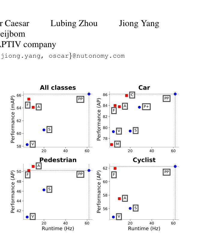
Figure 1: Bird’s eye view performance vs speed for our proposed PointPillars, PP method on the KITTI kitti test set. Lidar-only methods drawn as blue circles; lidar & vision methods drawn as red squares. Also drawn are top methods from the KITTI leaderboard: M: MV3D mv3d, A AVOD avod, C: ContFuse contfuse, V: VoxelNet voxelnet, F: Frustum PointNet frustum, S: SECOND second, P+ PIXOR++ hdnet. PointPillars outperforms all other lidar-only methods in terms of both speed and accuracy by a large margin. It also outperforms all fusion based method except on pedestrians. Similar performance is achieved on the 3D metric (Table 2).

图 1：所提 PointPillars（PP）在 KITTI kitti 测试集上的鸟瞰性能相对速度。仅激光雷达方法为蓝圆；激光雷达与视觉融合为红方。同时标出 KITTI 榜前列方法：M: MV3D mv3d，A: AVOD avod，C: ContFuse contfuse，V: VoxelNet voxelnet，F: Frustum PointNet frustum，S: SECOND second，P+: PIXOR++ hdnet。PointPillars 在速度与精度上大幅领先所有仅激光雷达方法；除行人外也优于所有融合方法。三维指标表现类似（表 2）。

1 Introduction

1 引言

Deploying autonomous vehicles (AVs) in urban environments poses a difficult technological challenge. Among other tasks, AVs need to detect and track moving objects such as vehicles, pedestrians, and cyclists in realtime. To achieve this, autonomous vehicles rely on several sensors out of which the lidar is arguably the most important. A lidar uses a laser scanner to measure the distance to the environment, thus generating a sparse point cloud representation. Traditionally, a lidar robotics pipeline interprets such point clouds as object detections through a bottom-up pipeline involving background subtraction, followed by spatiotemporal clustering and classification classic_lidar; himmelsbach2008lidar.

在城市环境部署自动驾驶车辆（AV）是艰巨的技术挑战。AV 需要实时检测并跟踪车辆、行人、骑行者等运动目标。为此依赖多种传感器，其中激光雷达 arguably 最为关键：用激光扫描测距，生成稀疏点云。传统激光雷达机器人管线通过背景减除、时空聚类与分类自底向上解释点云 classic_lidar；himmelsbach2008lidar。

Following the tremendous advances in deep learning methods for computer vision, a large body of literature has investigated to what extent this technology could be applied towards object detection from lidar point clouds voxelnet; hdnet; pixor; avod; mv3d; frustum; contfuse; second; complexyolo; roarnet. While there are many similarities between the modalities, there are two key differences: 1) the point cloud is a sparse representation, while an image is dense and 2) the point cloud is 3D, while the image is 2D. As a result object detection from point clouds does not trivially lend itself to standard image convolutional pipelines.

随着计算机视觉深度学习的巨大进展，大量工作探索把同类技术用于激光雷达点云目标检测 voxelnet；hdnet；pixor；avod；mv3d；frustum；contfuse；second；complexyolo；roarnet。模态之间有许多相似之处，但有两点关键差异：1）点云稀疏而图像稠密；2）点云是三维、图像是二维。因此点云目标检测不能 trivially 套用标准图像卷积管线。

Some early works focus on either using 3D convolutions engelcke2017vote3deep or a projection of the point cloud into the image fcl. Recent methods tend to view the lidar point cloud from a bird’s eye view mv3d; avod; voxelnet; pixor. This overhead perspective offers several advantages such as lack of scale ambiguity and the near lack of occlusion.

早期工作或使用三维卷积 engelcke2017vote3deep，或把点云投影到图像 fcl。近期方法更倾向从鸟瞰看激光雷达点云 mv3d；avod；voxelnet；pixor。俯视视角有若干优点：几乎没有尺度歧义，遮挡也近乎消失。

However, the bird’s eye view tends to be extremely sparse which makes direct application of convolutional neural networks impractical and inefficient. A common workaround to this problem is to partition the ground plane into a regular grid, for example 10 x 10 cm, and then perform a hand crafted feature encoding method on the points in each grid cell mv3d; avod; complexyolo; pixor. However, such methods may be sub-optimal since the hard-coded feature extraction method may not generalize to new configurations without significant engineering efforts. To address these issues, and building on the PointNet design developed by Qi et al. pointnet, VoxelNet voxelnet was one of the first methods to truly do end-to-end learning in this domain. VoxelNet divides the space into voxels, applies a PointNet to each voxel, followed by a 3D convolutional middle layer to consolidate the vertical axis, after which a 2D convolutional detection architecture is applied. While the VoxelNet performance is strong, the inference time, at $4.4~H\hskip-1.42262ptz$, is too slow to deploy in real time. Recently SECOND second improved the inference speed of VoxelNet but the 3D convolutions remain a bottleneck.

但鸟瞰往往极度稀疏，直接套 CNN 既不现实也低效。常见变通是把地面划成规则网格（例如 10×10 cm），再对每个格子内的点做手工特征编码 mv3d；avod；complexyolo；pixor。这类方法可能次优：硬编码特征提取未必能泛化到新配置，还要大量工程。为解决这些问题，并借鉴 Qi 等人提出的 PointNet pointnet，VoxelNet voxelnet 是该领域较早真正端到端学习的方法之一：把空间划成立方体素，对每个体素跑 PointNet，再经三维卷积中间层沿竖直轴压缩，最后接二维卷积检测架构。VoxelNet 性能强，但推理仅 $4.4~H\hskip-1.42262ptz$，难以实时部署。近期 SECOND second 提升了 VoxelNet 推理速度，三维卷积仍是瓶颈。

In this work we propose PointPillars: a method for object detection in 3D that enables end-to-end learning with only 2D convolutional layers. PointPillars uses a novel encoder that learn features on pillars (vertical columns) of the point cloud to predict 3D oriented boxes for objects. There are several advantages of this approach. First, by learning features instead of relying on fixed encoders, PointPillars can leverage the full information represented by the point cloud. Further, by operating on pillars instead of voxels there is no need to tune the binning of the vertical direction by hand. Finally, pillars are highly efficient because all key operations can be formulated as 2D convolutions which are extremely efficient to compute on a GPU. An additional benefit of learning features is that PointPillars requires no hand-tuning to use different point cloud configurations. For example, it can easily incorporate multiple lidar scans, or even radar point clouds.

本文提出 PointPillars：一种仅用二维卷积层即可端到端学习的三维目标检测方法。它用新颖编码器在点云的柱（竖直柱）上学习特征，预测目标的三维有向框。优势有几方面。其一，学习特征而非依赖固定编码器，能充分利用点云信息。其二，在柱上而非体素上操作，不必手工调节竖直方向分箱。其三，柱非常高效：关键运算都可写成 GPU 上极快的二维卷积。学习特征还有一个额外好处：换点云配置时无需手工调参，例如可轻松纳入多帧激光雷达，甚至雷达点云。

We evaluated our PointPillars network on the public KITTI detection challenges which require detection of cars, pedestrians, and cyclists in either the bird’s eye view (BEV) or 3D kitti. While our PointPillars network is trained using only lidar point clouds, it dominates the current state of the art including methods that use lidar and images, thus establishing new standards for performance on both BEV and 3D detection (Table 1 and Table 2). At the same time PointPillars runs at $62~H\hskip-1.42262ptz$, which is orders of magnitude faster than previous art. PointPillars further enables a trade off between speed and accuracy; in one setting we match state of the art performance at over $100~H\hskip-1.42262ptz$ (Figure 5). We have also released code (https://github.com/nutonomy/second.pytorch) that can reproduce our results.

我们在公开 KITTI 检测挑战上评估 PointPillars，需在鸟瞰（BEV）或三维中检测车、行人与骑行者 kitti。网络仅用激光雷达点云训练，却主导当时最优——包括同时用激光雷达与图像的方法，从而在 BEV 与三维检测上树立新标杆（表 1、表 2）。同时以 $62~H\hskip-1.42262ptz$ 运行，比以往方法快几个数量级。PointPillars 还允许在速度与精度间权衡；某一配置可在超过 $100~H\hskip-1.42262ptz$ 时匹配当时最优（图 5）。我们亦开源代码（https://github.com/nutonomy/second.pytorch）以复现结果。

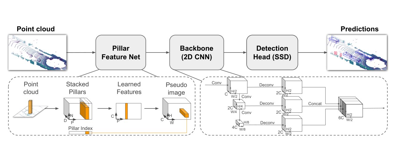
Figure 2: Network overview. The main components of the network are a Pillar Feature Network, Backbone, and SSD Detection Head. See Section 2 for more details. The raw point cloud is converted to a stacked pillar tensor and pillar index tensor. The encoder uses the stacked pillars to learn a set of features that can be scattered back to a 2D pseudo-image for a convolutional neural network. The features from the backbone are used by the detection head to predict 3D bounding boxes for objects. Note: here we show the backbone dimensions for the car network.

图 2：网络总览。主组件为柱特征网络、骨干与 SSD 检测头。细节见第 2 节。原始点云转为堆叠柱张量与柱索引张量。编码器利用堆叠柱学习特征，再散射回二维伪图像供 CNN 使用。骨干特征由检测头用于预测目标三维框。注：此处展示的是车辆网络的骨干尺寸。

1.1 Related Work

1.1 相关工作

We start by reviewing recent work in applying convolutional neural networks toward object detection in general, and then focus on methods specific to object detection from lidar point clouds.

我们先回顾把卷积神经网络用于一般目标检测的近期工作，再聚焦激光雷达点云目标检测的专用方法。

1.1.1 Object detection using CNNs

Starting with the seminal work of Girshick et al. girshick2014rich it was established that convolutional neural network (CNN) architectures are state of the art for detection in images. The series of papers that followed ren2015faster; he2017mask advocate a two-stage approach to this problem, where in the first stage a region proposal network (RPN) suggests candidate proposals. Cropped and resized versions of these proposals are then classified by a second stage network. Two-stage methods dominated the important vision benchmark datasets such as COCO coco over single-stage architectures originally proposed by Liu et al. ssd. In a single-stage architecture a dense set of anchor boxes is regressed and classified in a single stage into a set of predictions providing a fast and simple architecture. Recently Lin et al. retinanet convincingly argued that with their proposed focal loss function a single stage method is superior to two-stage methods, both in terms of accuracy and runtime. In this work, we use a single stage method.

1.1.1 基于 CNN 的目标检测

自 Girshick 等人 girshick2014rich 的开创工作起，CNN 架构已成为图像检测的主流。随后一系列论文 ren2015faster；he2017mask 主张两阶段：第一阶段区域提议网络（RPN）给出候选，裁剪缩放后再由第二阶段分类。两阶段方法在 COCO coco 等重要视觉基准上长期压过 Liu 等人 ssd 提出的单阶段架构。单阶段对稠密锚框一次回归与分类，结构快而简单。Lin 等人 retinanet 近期有力论证：配合他们提出的 focal loss，单阶段在精度与速度上均可优于两阶段。本文采用单阶段方法。

1.1.2 Object detection in lidar point clouds

Object detection in point clouds is an intrinsically three dimensional problem. As such, it is natural to deploy a 3D convolutional network for detection, which is the paradigm of several early works engelcke2017vote3deep; li20173d. While providing a straight-forward architecture, these methods are slow; e.g. Engelcke et al. engelcke2017vote3deep require $0.5s$ for inference on a single point cloud. Most recent methods improve the runtime by projecting the 3D point cloud either onto the ground plane avod; mv3d or the image plane fcl. In the most common paradigm the point cloud is organized in voxels and the set of voxels in each vertical column is encoded into a fixed-length, hand-crafted, feature encoding to form a pseudo-image which can be processed by a standard image detection architecture. Some notable works here include MV3D mv3d, AVOD avod, PIXOR pixor and Complex YOLO complexyolo which all use variations on the same fixed encoding paradigm as the first step of their architectures. The first two methods additionally fuse the lidar features with image features to create a multi-modal detector. The fusion step used in MV3D and AVOD forces them to use two-stage detection pipelines, while PIXOR and Complex YOLO use single stage pipelines.

1.1.2 激光雷达点云中的目标检测

点云目标检测本质上是三维问题。自然会部署三维卷积网络，这也是若干早期工作的范式 engelcke2017vote3deep；li20173d。架构直观，但慢：例如 Engelcke 等人 engelcke2017vote3deep 单帧点云推理需 $0.5s$。多数近期方法把三维点云投影到地面 avod；mv3d 或图像平面 fcl 以提速。最常见范式是把点云组织成体素，再把每根竖直柱中的体素编码成定长手工特征，形成伪图像，交给标准图像检测架构。代表作包括 MV3D mv3d、AVOD avod、PIXOR pixor 与 Complex YOLO complexyolo，它们都在架构第一步使用同一类固定编码变体。前两者还把激光雷达特征与图像特征融合，做成多模态检测器。MV3D 与 AVOD 的融合步骤迫使它们采用两阶段检测；PIXOR 与 Complex YOLO 则用单阶段。

In their seminal work Qi et al. pointnet; pointnetplusplus proposed a simple architecture, PointNet, for learning from unordered point sets, which offered a path to full end-to-end learning. VoxelNet voxelnet is one of the first methods to deploy PointNets for object detection in lidar point clouds. In their method, PointNets are applied to voxels which are then processed by a set of 3D convolutional layers followed by a 2D backbone and a detection head. This enables end-to-end learning, but like the earlier work that relied on 3D convolutions, VoxelNet is slow, requiring 225ms inference time ($4.4~H\hskip-1.42262ptz$) for a single point cloud. Another recent method, Frustum PointNet frustum, uses PointNets to segment and classify the point cloud in a frustum generated from projecting a detection on an image into 3D. Frustum PointNet’s achieved high benchmark performance compared to other fusion methods, but its multi-stage design makes end-to-end learning impractical. Very recently SECOND second offered a series of improvements to VoxelNet resulting in stronger performance and a much improved speed of $20~H\hskip-1.42262ptz$. However, they were unable to remove the expensive 3D convolutional layers.

Qi 等人 pointnet；pointnetplusplus 的开创工作提出处理无序点集的简单架构 PointNet，为完整端到端学习打开通路。VoxelNet voxelnet 是较早把 PointNet 用于激光雷达点云目标检测的方法之一：对体素施加 PointNet，再经一组三维卷积层，接二维骨干与检测头。这实现了端到端学习，但与依赖三维卷积的早期工作一样偏慢，单帧需 225ms（$4.4~H\hskip-1.42262ptz$）。另一近期方法 Frustum PointNet frustum 用 PointNet 对图像检测投影到三维形成的视锥内点云做分割与分类；相对其他融合方法基准表现高，但多阶段设计使端到端学习不现实。非常近期的 SECOND second 对 VoxelNet 做了一系列改进，性能更强、速度约 $20~H\hskip-1.42262ptz$，但仍未能去掉昂贵的三维卷积层。

1.2 Contributions

1.2 贡献

• • We propose a novel point cloud encoder and network, PointPillars, that operates on the point cloud to enable end-to-end training of a 3D object detection network.

• • 我们提出新颖的点云编码器与网络 PointPillars，在点云上操作，使三维目标检测网络可端到端训练。

• • We show how all computations on pillars can be posed as dense 2D convolutions which enables inference at $62~H\hskip-1.42262ptz$; a factor of 2-4 times faster than other methods.

• • 我们说明柱上全部计算都可写成稠密二维卷积，从而以 $62~H\hskip-1.42262ptz$ 推理，比其他方法快 2–4 倍。

• • We conduct experiments on the KITTI dataset and demonstrate state of the art results on cars, pedestrians, and cyclists on both BEV and 3D benchmarks.

• • 我们在 KITTI 上实验，于 BEV 与三维基准的车、行人、骑行者三类上取得当时最优结果。

• • We conduct several ablation studies to examine the key factors that enable a strong detection performance.

• • 我们做多项消融，考察支撑强检测表现的关键因素。

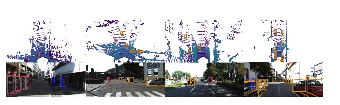
Figure 3: Qualitative analysis of KITTI results. We show a bird’s-eye view of the lidar point cloud (top), as well as the 3D bounding boxes projected into the image for clearer visualization. Note that our method only uses lidar. We show predicted boxes for car (orange), cyclist (red) and pedestrian (blue). Ground truth boxes are shown in gray. The orientation of boxes is shown by a line connected the bottom center to the front of the box.

图 3：KITTI 结果定性分析。上方为激光雷达点云鸟瞰，下方把三维框投影到图像以便可视化。注意我们的方法仅使用激光雷达。预测框：车（橙）、骑行者（红）、行人（蓝）；真值框为灰。框朝向用底边中心连到框前端的线表示。

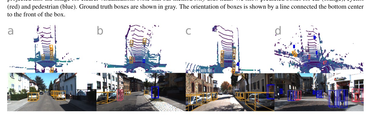
Figure 4: Failure cases on KITTI. Same visualize setup from Figure 3 but focusing on several common failure modes.

图 4：KITTI 上的失败案例。可视化设置同图 3，聚焦若干常见失败模式。

2 PointPillars Network

2 PointPillars 网络

PointPillars accepts point clouds as input and estimates oriented 3D boxes for cars, pedestrians and cyclists. It consists of three main stages (Figure 2): (1) A feature encoder network that converts a point cloud to a sparse pseudo-image; (2) a 2D convolutional backbone to process the pseudo-image into high-level representation; and (3) a detection head that detects and regresses 3D boxes.

PointPillars 以点云为输入，估计车、行人与骑行者的有向三维框。它包含三个主阶段（图 2）：(1) 特征编码器网络，把点云转为稀疏伪图像；(2) 二维卷积骨干，把伪图像处理成高层表示；(3) 检测头，检测并回归三维框。

2.1 Pointcloud to Pseudo-Image

2.1 点云到伪图像

To apply a 2D convolutional architecture, we first convert the point cloud to a pseudo-image.

为应用二维卷积架构，我们先把点云转为伪图像。

We denote by $l$ a point in a point cloud with coordinates $x$, $y$, $z$ and reflectance $r$. As a first step the point cloud is discretized into an evenly spaced grid in the x-y plane, creating a set of pillars $\mathcal{P}$ with $|\mathcal{P}|=B$. Note that there is no need for a hyper parameter to control the binning in the z dimension. The points in each pillar are then augmented with $x_{c}$, $y_{c}$, $z_{c}$, $x_{p}$ and $y_{p}$ where the $c$ subscript denotes distance to the arithmetic mean of all points in the pillar and the $p$ subscript denotes the offset from the pillar $x,y$ center. The augmented lidar point $l$ is now $D=9$ dimensional.

记点云中一点为 $l$，坐标 $x,y,z$ 与反射率 $r$。第一步在 x-y 平面把点云离散成均匀网格，得到柱集合 $\mathcal{P}$，满足 $|\mathcal{P}|=B$。注意 z 方向分箱无需超参。柱内各点再增广 $x_{c},y_{c},z_{c},x_{p},y_{p}$：$c$ 下标表示到柱内所有点算术均值的距离，$p$ 下标表示相对柱 $x,y$ 中心的偏移。增广后激光雷达点 $l$ 为 $D=9$ 维。

The set of pillars will be mostly empty due to sparsity of the point cloud, and the non-empty pillars will in general have few points in them. For example, at $0.16^{2}~m^{2}$ bins the point cloud from an HDL-64E Velodyne lidar has 6k-9k non-empty pillars in the range typically used in KITTI for $\sim 97\%$ sparsity. This sparsity is exploited by imposing a limit both on the number of non-empty pillars per sample ($P$) and on the number of points per pillar ($N$) to create a dense tensor of size $(D,P,N)$. If a sample or pillar holds too much data to fit in this tensor the data is randomly sampled. Conversely, if a sample or pillar has too little data to populate the tensor, zero padding is applied.

因点云稀疏，柱集合大多为空，非空柱一般点数也少。例如在 $0.16^{2}~m^{2}$ 分箱下，HDL-64E Velodyne 在 KITTI 常用范围内约有 6k–9k 非空柱，稀疏度约 97%。利用该稀疏性，对每样本非空柱数设上限 $P$、对每柱点数设上限 $N$，得到大小为 $(D,P,N)$ 的稠密张量。若样本或柱数据过多装不下，则随机采样；过少则零填充。

Next, we use a simplified version of PointNet where, for each point, a linear layer is applied followed by BatchNorm batchnorm and ReLU relu to generate a $(C,P,N)$ sized tensor. This is followed by a max operation over the channels to create an output tensor of size $(C,P)$. Note that the linear layer can be formulated as a 1x1 convolution across the tensor resulting in very efficient computation.

接着用简化版 PointNet：对每点施加线性层，再接 BatchNorm batchnorm 与 ReLU relu，得到 $(C,P,N)$ 张量；再沿通道做 max，输出 $(C,P)$。注意线性层可写成张量上的 1×1 卷积，计算非常高效。

Once encoded, the features are scattered back to the original pillar locations to create a pseudo-image of size $(C,H,W)$ where $H$ and $W$ indicate the height and width of the canvas.

编码完成后，特征按原柱位置散射回去，形成大小为 $(C,H,W)$ 的伪图像，$H,W$ 为画布高宽。

2.2 Backbone

2.2 骨干

We use a similar backbone as voxelnet and the structure is shown in Figure 2. The backbone has two sub-networks: one top-down network that produces features at increasingly small spatial resolution and a second network that performs upsampling and concatenation of the top-down features. The top-down backbone can be characterized by a series of blocks Block($S$, $L$, $F$). Each block operates at stride $S$ (measured relative to the original input pseudo-image). A block has $L$ 3x3 2D conv-layers with $F$ output channels, each followed by BatchNorm and a ReLU. The first convolution inside the layer has stride $\frac{S}{S_{in}}$ to ensure the block operates on stride $S$ after receiving an input blob of stride $S_{in}$. All subsequent convolutions in a block have stride 1.

我们采用与 voxelnet 类似的骨干，结构见图 2。骨干有两个子网络：一个自上而下、在越来越小空间分辨率上产出特征；另一个对自上而下特征上采样并拼接。自上而下骨干可用一系列块 Block($S$, $L$, $F$) 刻画。每块在步幅 $S$ 上工作（相对原始输入伪图像度量）。块内有 $L$ 个输出通道为 $F$ 的 3×3 二维卷积层，每层后接 BatchNorm 与 ReLU。层内第一个卷积步幅为 $\frac{S}{S_{in}}$，以保证在接收步幅 $S_{in}$ 的输入后块工作在步幅 $S$；其后卷积步幅均为 1。

The final features from each top-down block are combined through upsampling and concatenation as follows. First, the features are upsampled, Up($S_{in}$, $S_{out}$, $F$) from an initial stride $S_{in}$ to a final stride $S_{out}$ (both again measured wrt. original pseudo-image) using a transposed 2D convolution with $F$ final features. Next, BatchNorm and ReLU is applied to the upsampled features. The final output features are a concatenation of all features that originated from different strides.

各自上而下块的最终特征经上采样与拼接合并。先用转置二维卷积把特征从初始步幅 $S_{in}$ 上采样到最终步幅 $S_{out}$（均相对原始伪图像），记为 Up($S_{in}$, $S_{out}$, $F$)，得到 $F$ 维特征；再接 BatchNorm 与 ReLU。最终输出是来自不同步幅的全部特征的拼接。

2.3 Detection Head

2.3 检测头

In this paper, we use the Single Shot Detector (SSD) ssd setup to perform 3D object detection. Similar to SSD, we match the priorboxes to the ground truth using 2D Intersection over Union (IoU)  pascal. Bounding box height and elevation were not used for matching; instead given a 2D match, the height and elevation become additional regression targets.

本文用 Single Shot Detector（SSD） ssd 设定做三维目标检测。与 SSD 类似，用二维交并比（IoU） pascal 把先验框与真值匹配。匹配时不用框高与高程；给定二维匹配后，高与高程成为额外回归目标。

3 Implementation Details

3 实现细节

In this section we describe our network parameters and the loss function that we optimize for.

本节描述网络参数与所优化的损失函数。

3.1 Network

3.1 网络

Instead of pre-training our networks, all weights were initialized randomly using a uniform distribution as in heInit.

网络不做预训练，全部权重按 heInit 用均匀分布随机初始化。

The encoder network has $C=64$ output features. The car and pedestrian/cyclist backbones are the same except for the stride of the first block ($S=2$ for car, $S=1$ for pedestrian/cyclist). Both network consists of three blocks, Block1($S$, 4, C), Block2($2S$, 6, 2C), and Block3($4S$, 6, 4C). Each block is upsampled by the following upsampling steps: Up1($S$, $S$, 2C), Up2($2S$, $S$, 2C) and Up3($4S$, $S$, 2C). Then the features of Up1, Up2 and Up3 are concatenated together to create 6C features for the detection head.

编码器网络输出特征维 $C=64$。车辆与行人/骑行者骨干相同，仅第一块步幅不同（车辆 $S=2$，行人/骑行者 $S=1$）。两网络均含三块：Block1($S$, 4, C)、Block2($2S$, 6, 2C)、Block3($4S$, 6, 4C)。各块经如下上采样：Up1($S$, $S$, 2C)、Up2($2S$, $S$, 2C)、Up3($4S$, $S$, 2C)。再把 Up1、Up2、Up3 特征拼接，得到检测头用的 6C 维特征。

3.2 Loss

3.2 损失

We use the same loss functions introduced in SECOND second. Ground truth boxes and anchors are defined by $(x,y,z,w,l,h,\theta)$. The localization regression residuals between ground truth and anchors are defined by:

我们采用 SECOND second 引入的同一套损失。真值框与锚框由 $(x,y,z,w,l,h,\theta)$ 定义。真值与锚框之间的定位回归残差定义为：

$$\displaystyle\left.\begin{aligned} \Delta x&=\frac{x^{gt}-x^{a}}{d^{a}},\Delta y=\frac{y^{gt}-y^{a}}{d^{a}},\Delta z=\frac{z^{gt}-z^{a}}{h^{a}}\
\Delta w&=\log{\frac{w^{gt}}{w^{a}}},\Delta l=\log{\frac{l^{gt}}{l^{a}}},\Delta h=\log{\frac{h^{gt}}{h^{a}}}\
\Delta\theta&=\sin{\left(\theta^{gt}-\theta^{a}\right)},\end{aligned}\right.$$

where $x^{gt}$ and $x^{a}$ are respectively the ground truth and anchor boxes and $d^{a}=\sqrt{(w^{a})^{2}+(l^{a})^{2}}$. The total localization loss is:

其中 $x^{gt}$ 与 $x^{a}$ 分别表示真值与锚框，$d^{a}=\sqrt{(w^{a})^{2}+(l^{a})^{2}}$。总定位损失为：

$$\displaystyle\mathcal{L}_{loc}=\sum_{b\in(x,y,z,w,l,h,\theta)}\text{SmoothL1}\left(\Delta b\right)$$

Since the angle localization loss cannot distinguish flipped boxes, we use a softmax classification loss on the discretized directions second, $\mathcal{L}_{dir}$, which enables the network to learn the heading.

因角度定位损失无法区分翻转框，我们在离散朝向上使用 softmax 分类损失 second，$\mathcal{L}_{dir}$，使网络能学习航向。

For the object classification loss, we use the focal loss retinanet:

目标分类损失采用 focal loss retinanet：

$$\displaystyle\mathcal{L}_{cls}=-\alpha_{a}\left(1-p^{a}\right)^{\gamma}\log p^{a},$$

where $p^{a}$ is the class probability of an anchor. We use the original paper settings of $\alpha=0.25$ and $\gamma=2$. The total loss is therefore:

其中 $p^{a}$ 为锚框的类别概率。沿用原论文设定 $\alpha=0.25$、$\gamma=2$。因此总损失为：

$$\displaystyle\mathcal{L} \\ \displaystyle=\frac{1}{N_{pos}}\left(\beta_{loc}\mathcal{L}_{loc}+\beta_{cls}\mathcal{L}_{cls}+\beta_{dir}\mathcal{L}_{dir}\right),$$

where $N_{pos}$ is the number of positive anchors and $\beta_{loc}=2$, $\beta_{cls}=1$, and $\beta_{dir}=0.2$.

其中 $N_{pos}$ 为正锚框数，$\beta_{loc}=2$，$\beta_{cls}=1$，$\beta_{dir}=0.2$。

To optimize the loss function we use the Adam optimizer with an initial learning rate of $2*10^{-4}$ and decay the learning rate by a factor of $0.8$ every $15$ epochs and train for $160$ epochs. We use a batch size of 2 for validation set and 4 for our test submission.

优化采用 Adam，初始学习率 $2*10^{-4}$，每 15 个 epoch 衰减 0.8 倍，共训练 160 个 epoch。验证集 batch size 为 2，测试提交为 4。

Method	Modality	Speed (Hz)	mAP	Car	Pedestrian	Cyclist
Mod.	Easy	Mod.	Hard	Easy	Mod.	Hard	Easy	Mod.	Hard
MV3D mv3d	Lidar & Img.	2.8	N/A	86.02	76.90	68.49	N/A	N/A	N/A	N/A	N/A	N/A
Cont-Fuse contfuse	Lidar & Img.	16.7	N/A	88.81	85.83	77.33	N/A	N/A	N/A	N/A	N/A	N/A
Roarnet roarnet	Lidar & Img.	10	N/A	88.20	79.41	70.02	N/A	N/A	N/A	N/A	N/A	N/A
AVOD-FPN avod	Lidar & Img.	10	64.11	88.53	83.79	77.90	58.75	51.05	47.54	68.09	57.48	50.77
F-PointNet frustum	Lidar & Img.	5.9	65.39	88.70	84.00	75.33	58.09	50.22	47.20	75.38	61.96	54.68
HDNET hdnet	Lidar & Map	20	N/A	89.14	86.57	78.32	N/A	N/A	N/A	N/A	N/A	N/A
PIXOR++ hdnet	Lidar	35	N/A	89.38	83.70	77.97	N/A	N/A	N/A	N/A	N/A	N/A
VoxelNet voxelnet	Lidar	4.4	58.25	89.35	79.26	77.39	46.13	40.74	38.11	66.70	54.76	50.55
SECOND second	Lidar	20	60.56	88.07	79.37	77.95	55.10	46.27	44.76	73.67	56.04	48.78
PointPillars	Lidar	62	66.19	88.35	86.10	79.83	58.66	50.23	47.19	79.14	62.25	56.00

Table 1: Results on the KITTI test BEV detection benchmark.

Method	Modality	Speed (Hz)	mAP	Car	Pedestrian	Cyclist
Mod.	Easy	Mod.	Hard	Easy	Mod.	Hard	Easy	Mod.	Hard
MV3D mv3d	Lidar & Img.	2.8	N/A	86.02	76.90	68.49	N/A	N/A	N/A	N/A	N/A	N/A
Cont-Fuse contfuse	Lidar & Img.	16.7	N/A	88.81	85.83	77.33	N/A	N/A	N/A	N/A	N/A	N/A
Roarnet roarnet	Lidar & Img.	10	N/A	88.20	79.41	70.02	N/A	N/A	N/A	N/A	N/A	N/A
AVOD-FPN avod	Lidar & Img.	10	64.11	88.53	83.79	77.90	58.75	51.05	47.54	68.09	57.48	50.77
F-PointNet frustum	Lidar & Img.	5.9	65.39	88.70	84.00	75.33	58.09	50.22	47.20	75.38	61.96	54.68
HDNET hdnet	Lidar & Map	20	N/A	89.14	86.57	78.32	N/A	N/A	N/A	N/A	N/A	N/A
PIXOR++ hdnet	Lidar	35	N/A	89.38	83.70	77.97	N/A	N/A	N/A	N/A	N/A	N/A
VoxelNet voxelnet	Lidar	4.4	58.25	89.35	79.26	77.39	46.13	40.74	38.11	66.70	54.76	50.55
SECOND second	Lidar	20	60.56	88.07	79.37	77.95	55.10	46.27	44.76	73.67	56.04	48.78
PointPillars	Lidar	62	66.19	88.35	86.10	79.83	58.66	50.23	47.19	79.14	62.25	56.00

表 1：KITTI 测试集 BEV 检测基准结果。

Method	Modality	Speed (Hz)	mAP	Car	Pedestrian	Cyclist
Mod.	Easy	Mod.	Hard	Easy	Mod.	Hard	Easy	Mod.	Hard
MV3D mv3d	Lidar & Img.	2.8	N/A	71.09	62.35	55.12	N/A	N/A	N/A	N/A	N/A	N/A
Cont-Fuse contfuse	Lidar & Img.	16.7	N/A	82.54	66.22	64.04	N/A	N/A	N/A	N/A	N/A	N/A
Roarnet roarnet	Lidar & Img.	10	N/A	83.71	73.04	59.16	N/A	N/A	N/A	N/A	N/A	N/A
AVOD-FPN avod	Lidar & Img.	10	55.62	81.94	71.88	66.38	50.80	42.81	40.88	64.00	52.18	46.61
F-PointNet frustum	Lidar & Img.	5.9	57.35	81.20	70.39	62.19	51.21	44.89	40.23	71.96	56.77	50.39
VoxelNet voxelnet	Lidar	4.4	49.05	77.47	65.11	57.73	39.48	33.69	31.5	61.22	48.36	44.37
SECOND second	Lidar	20	56.69	83.13	73.66	66.20	51.07	42.56	37.29	70.51	53.85	46.90
PointPillars	Lidar	62	59.20	79.05	74.99	68.30	52.08	43.53	41.49	75.78	59.07	52.92

Table 2: Results on the KITTI test 3D detection benchmark.

Method	Modality	Speed (Hz)	mAP	Car	Pedestrian	Cyclist
Mod.	Easy	Mod.	Hard	Easy	Mod.	Hard	Easy	Mod.	Hard
MV3D mv3d	Lidar & Img.	2.8	N/A	71.09	62.35	55.12	N/A	N/A	N/A	N/A	N/A	N/A
Cont-Fuse contfuse	Lidar & Img.	16.7	N/A	82.54	66.22	64.04	N/A	N/A	N/A	N/A	N/A	N/A
Roarnet roarnet	Lidar & Img.	10	N/A	83.71	73.04	59.16	N/A	N/A	N/A	N/A	N/A	N/A
AVOD-FPN avod	Lidar & Img.	10	55.62	81.94	71.88	66.38	50.80	42.81	40.88	64.00	52.18	46.61
F-PointNet frustum	Lidar & Img.	5.9	57.35	81.20	70.39	62.19	51.21	44.89	40.23	71.96	56.77	50.39
VoxelNet voxelnet	Lidar	4.4	49.05	77.47	65.11	57.73	39.48	33.69	31.5	61.22	48.36	44.37
SECOND second	Lidar	20	56.69	83.13	73.66	66.20	51.07	42.56	37.29	70.51	53.85	46.90
PointPillars	Lidar	62	59.20	79.05	74.99	68.30	52.08	43.53	41.49	75.78	59.07	52.92

表 2：KITTI 测试集三维检测基准结果。

Method	Modality	Speed (Hz)	mAOS	Car	Pedestrian	Cyclist
Mod.	Easy	Mod.	Hard	Easy	Mod.	Hard	Easy	Mod.	Hard
SubCNN xiang2017subcategory	Img.	0.5	72.71	90.61	88.43	78.63	78.33	66.28	61.37	71.39	63.41	56.34
AVOD-FPN avod	Lidar & Img.	10	63.19	89.95	87.13	79.74	53.36	44.92	43.77	67.61	57.53	54.16
SECOND second	Lidar	20	54.53	87.84	81.31	71.95	51.56	43.51	38.78	80.97	57.20	55.14
PointPillars	Lidar	62	68.86	90.19	88.76	86.38	58.05	49.66	47.88	82.43	68.16	61.96

Table 3: Results on the KITTI test average orientation similarity (AOS) detection benchmark. SubCNN is the best performing image only method, while AVOD-FPN, SECOND, and PointPillars are the only 3D object detectors that predict orientation.

Method	Modality	Speed (Hz)	mAOS	Car	Pedestrian	Cyclist
Mod.	Easy	Mod.	Hard	Easy	Mod.	Hard	Easy	Mod.	Hard
SubCNN xiang2017subcategory	Img.	0.5	72.71	90.61	88.43	78.63	78.33	66.28	61.37	71.39	63.41	56.34
AVOD-FPN avod	Lidar & Img.	10	63.19	89.95	87.13	79.74	53.36	44.92	43.77	67.61	57.53	54.16
SECOND second	Lidar	20	54.53	87.84	81.31	71.95	51.56	43.51	38.78	80.97	57.20	55.14
PointPillars	Lidar	62	68.86	90.19	88.76	86.38	58.05	49.66	47.88	82.43	68.16	61.96

表 3：KITTI 测试集平均朝向相似度（AOS）检测基准。SubCNN 是表现最好的仅图像方法；AVOD-FPN、SECOND 与 PointPillars 是仅有的预测朝向的三维目标检测器。

4 Experimental setup

4 实验设置

In this section we present our experimental setup, including dataset, experimental settings and data augmentation.

本节给出实验设置，包括数据集、实验配置与数据增强。

4.1 Dataset

4.1 数据集

All experiments use the KITTI object detection benchmark dataset kitti, which consists of samples that have both lidar point clouds and images. We only train on lidar point clouds, but compare with fusion methods that use both lidar and images. The samples are originally divided into 7481 training and 7518 testing samples. For experimental studies we split the official training into 3712 training samples and 3769 validation samples chen20153d, while for our test submission we created a minival set of 784 samples from the validation set and trained on the remaining 6733 samples. The KITTI benchmark requires detections of cars, pedestrians, and cyclists. Since the ground truth objects were only annotated if they are visible in the image, we follow the standard convention mv3d; voxelnet of only using lidar points that project into the image. Following the standard literature practice on KITTI avod; voxelnet; second, we train one network for cars and one network for both pedestrians and cyclists.

全部实验使用 KITTI 目标检测基准数据集 kitti，样本同时含激光雷达点云与图像。我们只在激光雷达点云上训练，但与同时用激光雷达和图像的融合方法比较。原始划分为 7481 训练、7518 测试样本。实验研究中把官方训练集拆成 3712 训练与 3769 验证 chen20153d；测试提交则从验证集划出 784 样本的 minival，在余下 6733 样本上训练。KITTI 基准要求检测车、行人与骑行者。由于真值目标仅在图像可见时标注，我们遵循惯例 mv3d；voxelnet，只用投影到图像内的激光雷达点。按 KITTI 文献惯例 avod；voxelnet；second，为车辆训练一个网络，为行人与骑行者共用另一个网络。

4.2 Settings

4.2 配置

Unless explicitly varied in an experimental study, we use an xy resolution: 0.16 m, max number of pillars ($P$): 12000, and max number of points per pillar ($N$): 100.

除非在某项实验中显式改动，我们使用 xy 分辨率 0.16 m、最大柱数 $P=12000$、每柱最大点数 $N=100$。

We use the same anchors and matching strategy as voxelnet. Each class anchor is described by a width, length, height, and z center, and is applied at two orientations: 0 and 90 degrees. Anchors are matched to ground truth using the 2D IoU with the following rules. A positive match is either the highest with a ground truth box, or above the positive match threshold, while a negative match is below the negative threshold. All other anchors are ignored in the loss.

锚框与匹配策略与 voxelnet 相同。每类锚框由宽、长、高与 z 中心描述，并在 0° 与 90° 两种朝向上施加。用二维 IoU 把锚框与真值匹配：正匹配为与某真值框 IoU 最高或高于正阈值；负匹配低于负阈值；其余锚框在损失中忽略。

At inference time we apply axis aligned non maximum suppression (NMS) with an overlap threshold of $0.5$ IoU. This provides similar performance compared to rotational NMS, but is much faster.

推理时做轴对齐非极大值抑制（NMS），重叠阈值为 $0.5$ IoU。相对旋转 NMS 性能相近，但快得多。

Car.

The x, y, z range is [(0, 70.4), (-40, 40), (-3, 1)] meters respectively. The car anchor has width, length, and height of (1.6, 3.9, 1.5) m with a z center of -1 m. Matching uses positive and negative thresholds of 0.6 and 0.45.

车辆。

x、y、z 范围分别为 [(0, 70.4), (-40, 40), (-3, 1)] 米。车辆锚框宽、长、高为 (1.6, 3.9, 1.5) m，z 中心 -1 m。匹配正/负阈值为 0.6 与 0.45。

Pedestrian & Cyclist.

The x, y, z range of [(0, 48), (-20, 20), (-2.5, 0.5)] meters respectively. The pedestrian anchor has width, length, and height of (0.6, 0.8, 1.73) meters with a z center of -0.6 meters, while the cyclist anchor has width, length, and height of (0.6, 1.76, 1.73) meters with a z center of -0.6 meters. Matching uses positive and negative thresholds of 0.5 and 0.35.

行人与骑行者。

x、y、z 范围分别为 [(0, 48), (-20, 20), (-2.5, 0.5)] 米。行人锚框宽、长、高 (0.6, 0.8, 1.73) m，z 中心 -0.6 m；骑行者锚框 (0.6, 1.76, 1.73) m，z 中心 -0.6 m。匹配正/负阈值为 0.5 与 0.35。

4.3 Data Augmentation

4.3 数据增强

Data augmentation is critical for good performance on the KITTI benchmark second; pixor; mv3d.

数据增强对 KITTI 基准上取得好结果至关重要 second；pixor；mv3d。

First, following SECOND second, we create a lookup table of the ground truth 3D boxes for all classes and the associated point clouds that falls inside these 3D boxes. Then for each sample, we randomly select $15,0,8$ ground truth samples for cars, pedestrians, and cyclists respectively and place them into the current point cloud. We found these settings to perform better than the proposed settings second.

首先，沿用 SECOND second，为各类真值三维框及其框内点云建查找表。对每个样本，分别随机选取 15、0、8 个车、行人、骑行者真值样本放入当前点云。我们发现这些设定优于 second 原先建议。

Next, all ground truth boxes are individually augmented. Each box is rotated (uniformly drawn from $[-\pi/20,\pi/20]$) and translated (x, y, and z independently drawn from $\mathcal{N}(0,0.25)$) to further enrich the training set.

接着对每个真值框单独增强：旋转（从 $[-\pi/20,\pi/20]$ 均匀采样）与平移（x、y、z 独立从 $\mathcal{N}(0,0.25)$ 采样），进一步丰富训练集。

Finally, we perform two sets of global augmentations that are jointly applied to the point cloud and all boxes. First, we apply random mirroring flip along the x axis pixor, then a global rotation and scaling voxelnet; second. Finally, we apply a global translation with x, y, z drawn from $\mathcal{N}(0,0.2)$ to simulate localization noise.

最后做两组全局增强，同时作用于点云与全部框：先沿 x 轴随机镜像翻转 pixor，再做全局旋转与缩放 voxelnet；second；最后用从 $\mathcal{N}(0,0.2)$ 采样的 x、y、z 做全局平移，以模拟定位噪声。

5 Results

5 结果

In this section we present results of our PointPillars method and compare to the literature.

本节给出 PointPillars 结果并与文献比较。

Quantitative Analysis.

All detection results are measured using the official KITTI evaluation detection metrics which are: bird’s eye view (BEV), 3D, 2D, and average orientation similarity (AOS). The 2D detection is done in the image plane and average orientation similarity assesses the average orientation (measured in BEV) similarity for 2D detections. The KITTI dataset is stratified into easy, moderate, and hard difficulties, and the official KITTI leaderboard is ranked by performance on moderate.

定量分析。

全部检测结果按官方 KITTI 评估指标度量：鸟瞰（BEV）、三维、二维与平均朝向相似度（AOS）。二维检测在图像平面进行；平均朝向相似度评估二维检测匹配的平均朝向（在 BEV 中度量）。KITTI 数据集按易、中、难分层，官方排行榜以中等难度表现为准。

As shown in Table 1 and Table 2, PointPillars outperforms all published methods with respect to mean average precision (mAP). Compared to lidar-only methods, PointPillars achieves better results across all classes and difficulty strata except for the easy car stratum. It also outperforms fusion based methods on cars and cyclists.

如表 1 与表 2 所示，PointPillars 在平均精度（mAP）上超过所有已发表方法。相对仅激光雷达方法，除车辆易档外，在各类与各难度层均更好；相对融合方法，在车与骑行者上也更优。

While PointPillars predicts 3D oriented boxes, the BEV and 3D metrics do not take orientation into account. Orientation is evaluated using AOS kitti, which requires projecting the 3D box into the image, performing 2D detection matching, and then assessing the orientation of these matches. The performance of PointPillars on AOS significantly exceeds in all strata as compared to the only two 3D detection methods avod; second that predict oriented boxes (Table 3). In general, image only methods perform best on 2D detection since the 3D projection of boxes into the image can result in loose boxes depending on the 3D pose. Despite this, PointPillars moderate cyclist AOS of 68.16 outperforms the best image based method xiang2017subcategory.

虽 PointPillars 预测有向三维框，BEV 与三维指标并不考虑朝向。朝向用 AOS kitti 评估：需把三维框投影到图像、做二维检测匹配，再评估这些匹配的朝向。相对仅有的两个预测有向框的三维检测方法 avod；second，PointPillars 在 AOS 各层均显著更高（表 3）。一般仅图像方法在二维检测上最好，因为三维框投影到图像会随姿态产生松散框。尽管如此，PointPillars 骑行者中等 AOS 达 68.16，超过最佳仅图像方法 xiang2017subcategory。

For comparison to other methods on val, we note that our network achieved BEV AP of ($87.98$, $63.55$, $69.71$) and 3D AP of ($77.98$, $57.86$, $66.02$) for the moderate strata of cars, pedestrians, and cyclists respectively.

与 val 上其他方法比较时，我们网络在车、行人、骑行者中等难度上分别达到 BEV AP（87.98，63.55，69.71）与三维 AP（77.98，57.86，66.02）。

Qualitative Analysis.

We provide qualitative results in Figure 3 and 4. While we only train on lidar point clouds, for ease of interpretation we visualize the 3D bounding box predictions from the BEV and image perspective. Figure 3 shows our detection results, with tight oriented 3D bounding boxes. The predictions for cars are particularly accurate and common failure modes include false negatives on difficult samples (partially occluded or faraway objects) or false positives on similar classes (vans or trams). Detecting pedestrians and cyclists is more challenging and leads to some interesting failure modes. Pedestrians and cyclists are commonly misclassified as each other (see Figure 4a for a standard example and Figure 4d for the combination of pedestrian and table classified as a cyclist). Additionally, pedestrians are easily confused with narrow vertical features of the environment such as poles or tree trunks (see Figure 4b). In some cases we correctly detect objects that are missing in the ground truth annotations (see Figure 4c).

定性分析。

图 3 与图 4 给出定性结果。虽只在激光雷达点云上训练，为便于解读，我们从 BEV 与图像视角可视化三维框预测。图 3 显示检测结果，有向三维框贴合紧密。车辆预测尤其准确；常见失败包括难样本（部分遮挡或远处）漏检，或对相似类别（厢式车、有轨电车）误检。行人与骑行者更难，会出现有趣失败模式：二者常被互相误分类（见图 4a 的典型例子，以及图 4d 中行人加桌子被当成骑行者）。此外行人易与环境中细长竖直结构（杆、树干）混淆（见图 4b）。有时我们正确检出真值标注缺失的目标（见图 4c）。

6 Realtime Inference

6 实时推理

As indicated by our results (Table 1 and Figure 5), PointPillars represent a significant improvement in terms of inference runtime. In this section we break down our runtime and consider the different design choices that enabled this speedup. We focus on the car network, but the pedestrian and bicycle network runs at a similar speed since the smaller range cancels the effect of the backbone operating at lower strides. All runtimes are measured on a desktop with an Intel i7 CPU and a 1080ti GPU.

如表 1 与图 5 所示，PointPillars 在推理耗时上有显著改进。本节拆解运行时间，并讨论促成加速的设计选择。我们聚焦车辆网络；行人与自行车网络速度相近，因为更小范围抵消了骨干在更低步幅上工作的影响。全部耗时在配备 Intel i7 CPU 与 1080ti GPU 的台式机上测得。

The main inference steps are as follows. First, the point cloud is loaded and filtered based on range and visibility in the images ($1.4~ms$). Then, the points are organized in pillars and decorated ($2.7~ms$). Next, the PointPillar tensor is uploaded to the GPU ($2.9~ms$), encoded ($1.3~ms$), scattered to the pseudo-image ($0.1~ms$), and processed by the backbone and detection heads ($7.7~ms$). Finally NMS is applied on the CPU ($0.1~ms$) for a total runtime of $16.2~ms$.

主要推理步骤如下。先加载点云并按距离与图像可见性过滤（$1.4~ms$）；再把点组织成柱并做装饰（$2.7~ms$）；接着把 PointPillar 张量上传 GPU（$2.9~ms$）、编码（$1.3~ms$）、散射到伪图像（$0.1~ms$），由骨干与检测头处理（$7.7~ms$）；最后在 CPU 上做 NMS（$0.1~ms$），总耗时 $16.2~ms$。

Encoding.

The key design to enable this runtime is the PointPilar encoding. For example, at $1.3~ms$ it is 2 orders of magnitude faster than the VoxelNet encoder ($190~ms$) voxelnet. Recently, SECOND proposed a faster sparse version of the VoxelNet encoder for a total network runtime of $50~ms$. They did not provide a runtime analysis, but since the rest of their architecture is similar to ours, it suggests that the encoder is still significantly slower; in their open source implementation[^1] the encoder requires $48~ms$.

编码。

实现该耗时的关键设计是 PointPillar 编码。例如 $1.3~ms$ 比 VoxelNet 编码器（$190~ms$） voxelnet 快两个数量级。近期 SECOND 提出更快的稀疏 VoxelNet 编码器，整网运行约 $50~ms$。他们未给分项耗时，但因其余架构与我们相近，可推断编码器仍明显更慢；其开源实现[^1] 中编码器需 $48~ms$。

Slimmer Design.

We opt for a single PointNet in our encoder, compared to 2 sequential PointNets suggested by voxelnet. This reduced our runtime by $2.5~ms$ in our PyTorch runtime. The number of dimensions of the first block were also lowered $64$ to match the encoder output size, which reduced the runtime by $4.5~ms$. Finally, we saved another $3.9~ms$ by cutting the output dimensions of the upsampled feature layers by half to $128$. Neither of these changes affected detection performance.

更瘦设计。

编码器只用单个 PointNet，而 voxelnet 建议两个串联 PointNet。这使我们的 PyTorch 运行时减少 $2.5~ms$。第一块通道数也降到 $64$ 以匹配编码器输出，再省 $4.5~ms$。最后把上采样特征层输出维砍半到 $128$，再省 $3.9~ms$。这些改动均未影响检测性能。

TensorRT.

While all our experiments were performed in PyTorch pytorch, the final GPU kernels for encoding, backbone and detection head were built using NVIDIA TensorRT, which is a library for optimized GPU inference. Switching to TensorRT gave a $45.5\%$ speedup from the PyTorch pipeline which runs at $42.4~H\hskip-1.42262ptz$.

TensorRT。

虽全部实验在 PyTorch pytorch 中完成，编码、骨干与检测头的最终 GPU 核用 NVIDIA TensorRT 构建，这是面向优化 GPU 推理的库。切换到 TensorRT 相对以 $42.4~H\hskip-1.42262ptz$ 运行的 PyTorch 管线带来 45.5% 加速。

The Need for Speed.

As seen in Figure 5, PointPillars can achieve $105~H\hskip-1.42262ptz$ with limited loss of accuracy. While it could be argued that such runtime is excessive since a lidar typically operates at $20~H\hskip-1.42262ptz$, there are two key things to keep in mind. First, due to an artifact of the KITTI ground truth annotations, only lidar points which projected into the front image are utilized, which is only $\sim 10\%$ of the entire point cloud. However, an operational AV needs to view the full environment and process the complete point cloud, significantly increasing all aspects of the runtime. Second, timing measurements in the literature are typically done on a high-power desktop GPU. However, an operational AV may instead use embedded GPUs or embedded compute which may not have the same throughput.

为何需要速度。

如图 5，PointPillars 可在精度损失有限时达到 $105~H\hskip-1.42262ptz$。或许有人认为激光雷达通常 $20~H\hskip-1.42262ptz$ 工作，如此高帧率多余，但有两点需记住。其一，因 KITTI 真值标注的 artifact，只用投影到前视图像的激光雷达点，约占整幅点云的 $\sim 10\%$；实际运营 AV 需观察全环境并处理完整点云，会显著拉高各方面耗时。其二，文献测时通常用高功率桌面 GPU；运营 AV 更可能用嵌入式 GPU 或嵌入式算力，吞吐未必相同。

7 Ablation Studies

7 消融实验

In this section we provide ablation studies and discuss our design choices compared to the recent literature.

本节给出消融，并讨论相对近期文献的设计选择。

7.1 Spatial Resolution

7.1 空间分辨率

A trade-off between speed and accuracy can be achieved by varying the size of the spatial binning. Smaller pillars allow finer localization and lead to more features, while larger pillars are faster due to fewer non-empty pillars (speeding up the encoder) and a smaller pseudo-image (speeding up the CNN backbone). To quantify this effect we performed a sweep across grid sizes. From Figure 5 it is clear that the larger bin sizes lead to faster networks; at $0.28^{2}$ we achieve $105~H\hskip-1.42262ptz$ at similar performance to previous methods. The decrease in performance was mainly due to the pedestrian and cyclist classes, while car performance was stable across the bin sizes.

通过改变空间分箱大小可在速度与精度间权衡。更小的柱利于更精细定位、特征更多；更大的柱因非空柱更少（编码更快）且伪图像更小（CNN 骨干更快）而更快。为量化该效应，我们扫过网格尺寸。由图 5 可见，更大分箱带来更快网络；在 $0.28^{2}$ 时以接近以往方法的精度达到 $105~H\hskip-1.42262ptz$。性能下降主要来自行人与骑行者；车辆性能在各分箱尺寸上较稳。

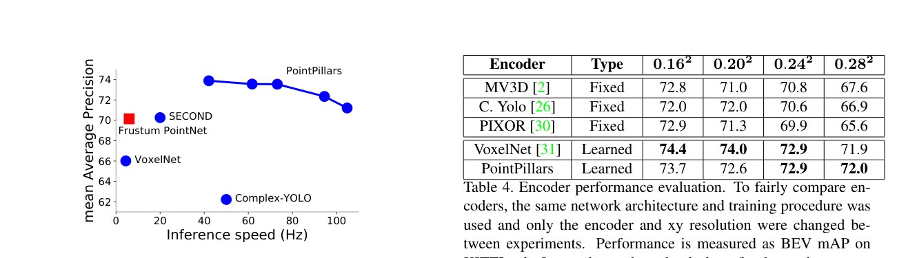
Figure 5: BEV detection performance (mAP) vs speed (Hz) on the KITTI kitti val set across pedestrians, bicycles and cars. Blue circles indicate lidar only methods, red squares indicate methods that use lidar & vision. Different operating points were achieved by using pillar grid sizes in $\{0.12^{2},0.16^{2},0.2^{2},0.24^{2},0.28^{2}\}$ $m^{2}$. The number of max-pillars was varied along with the resolution and set to $16000,12000,12000,8000,8000$ respectively.

图 5：KITTI kitti 验证集上行人、自行车与车辆的 BEV 检测性能（mAP）相对速度（Hz）。蓝圆为仅激光雷达方法，红方为激光雷达与视觉方法。工作点通过柱网格尺寸 $\{0.12^{2},0.16^{2},0.2^{2},0.24^{2},0.28^{2}\}$ $m^{2}$ 取得。最大柱数随分辨率变化，分别设为 $16000,12000,12000,8000,8000$。

7.2 Per Box Data Augmentation

7.2 逐框数据增强

Both VoxelNet voxelnet and SECOND second recommend extensive per box augmentation. However, in our experiments, minimal box augmentation worked better. In particular, the detection performance for pedestrians degraded significantly with more box augmentation. Our hypothesis is that the introduction of ground truth sampling mitigates the need for extensive per box augmentation.

VoxelNet voxelnet 与 SECOND second 都建议大量逐框增强。但我们实验中，轻度框增强效果更好。尤其行人检测在更强框增强下显著变差。我们的假设是：引入真值采样后，减轻了对大量逐框增强的依赖。

7.3 Point Decorations

7.3 点装饰

During the lidar point decoration step, we perform the VoxelNet voxelnet decorations plus two additional decorations: $x_{p}$ and $y_{p}$ which are the $x$ and $y$ offset from the pillar $x,y$ center. These extra decorations added 0.5 mAP to final detection performance and provided more reproducible experiments.

在激光雷达点装饰步骤，我们做 VoxelNet voxelnet 装饰，并额外加两项：$x_{p}$ 与 $y_{p}$，即相对柱 $x,y$ 中心的偏移。这些额外装饰为最终检测性能贡献约 0.5 mAP，并使实验更可复现。

7.4 Encoding

7.4 编码

To assess the impact of the proposed PointPillar encoding in isolation, we implemented several encoders in the official codebase of SECOND second. For details on each encoding, we refer to the original papers.

为单独评估所提 PointPillar 编码的影响，我们在 SECOND second 官方代码库中实现了若干编码器。各编码细节见原论文。

Encoder	Type	$\mathbf{0.16^{2}}$	$\mathbf{0.20^{2}}$	$\mathbf{0.24^{2}}$	$\mathbf{0.28^{2}}$
MV3D mv3d	Fixed	72.8	71.0	70.8	67.6
C. Yolo complexyolo	Fixed	72.0	72.0	70.6	66.9
PIXOR pixor	Fixed	72.9	71.3	69.9	65.6
VoxelNet voxelnet	Learned	74.4	74.0	72.9	71.9
PointPillars	Learned	73.7	72.6	72.9	72.0

Table 4: Encoder performance evaluation. To fairly compare encoders, the same network architecture and training procedure was used and only the encoder and xy resolution were changed between experiments. Performance is measured as BEV mAP on KITTI val. Learned encoders clearly beat fixed encoders, especially at larger resolutions.

Encoder	Type	$\mathbf{0.16^{2}}$	$\mathbf{0.20^{2}}$	$\mathbf{0.24^{2}}$	$\mathbf{0.28^{2}}$
MV3D mv3d	Fixed	72.8	71.0	70.8	67.6
C. Yolo complexyolo	Fixed	72.0	72.0	70.6	66.9
PIXOR pixor	Fixed	72.9	71.3	69.9	65.6
VoxelNet voxelnet	Learned	74.4	74.0	72.9	71.9
PointPillars	Learned	73.7	72.6	72.9	72.0

表 4：编码器性能评估。为公平比较，使用相同网络架构与训练流程，仅改编码器与 xy 分辨率。性能为 KITTI val 上 BEV mAP。学习编码器在各分辨率上明显优于固定编码器，大分辨率下差距更大。

As shown in Table 4, learning the feature encoding is strictly superior to fixed encoders across all resolution. This is expected as most successful deep learning architectures are trained end-to-end. Further, the differences increase with larger bin sizes where the lack of expressive power of the fixed encoders are accentuated due to a larger point cloud in each pillar. Among the learned encoders VoxelNet is marginally stronger than PointPillars. However, this is not a fair comparison, since the VoxelNet encoder is orders of magnitude slower and has orders of magnitude more parameters. When the comparison is made for a similar inference time, it is clear that PointPillars offers a better operating point (Figure 5).

如表 4，学习特征编码在所有分辨率上严格优于固定编码器。这符合预期：多数成功深度学习架构都是端到端训练。进一步，差距随分箱变大而扩大——每柱点云更多时，固定编码器表达力不足更突出。学习编码器中 VoxelNet 略强于 PointPillars。但这不公平：VoxelNet 编码器慢几个数量级、参数也多几个数量级。在相近推理时间下比较时，PointPillars 工作点更好（图 5）。

There are a few curious aspects of Table 4. First, despite notes in the original papers that their encoder only works on cars, we found that the MV3D mv3d and PIXOR pixor encoders can learn pedestrians and cyclists quite well. Second, our implementations beat the respective published results by a large margin ($1-10$ mAP). While this is not an apples to apples comparison since we only used the respective encoders and not the full network architectures, the performance difference is noteworthy. We see several potential reasons. For VoxelNet and SECOND we suspect the boost in performance comes from improved data augmentation hyperparameters as discussed in Section 7.2. Among the fixed encoders, roughly half the performance increase can be explained by the introduction of ground truth database sampling second, which we found to boost the mAP by around $3\%$ mAP. The remaining differences are likely due to a combination of multiple hyperparameters including network design (number of layers, type of layers, whether to use a feature pyramid); anchor box design (or lack thereof pixor); localization loss with respect to 3D and angle; classification loss; optimizer choices (SGD vs Adam, batch size); and more. However, a more careful study is needed to isolate each cause and effect.

表 4 还有几点值得注意。其一，尽管原论文称其编码器只适用于车，我们发现 MV3D mv3d 与 PIXOR pixor 编码器也能较好学习行人与骑行者。其二，我们的实现大幅超过各自已发表结果（1–10 mAP）。这并非严格苹果对苹果，因为我们只用了各自的编码器而非完整网络架构，但性能差距值得关注。可能原因有几个。对 VoxelNet 与 SECOND，我们怀疑提升来自第 7.2 节讨论的改进数据增强超参。固定编码器中，约一半提升可归因于引入真值数据库采样 second——我们发现它大约提升 3% mAP。其余差异很可能来自多种超参组合：网络设计（层数、层类型、是否用特征金字塔）；锚框设计（或 pixor 那样不用锚框）；相对三维与角度的定位损失；分类损失；优化器选择（SGD vs Adam、batch size）等。不过需要更仔细的研究才能隔离各因果。

8 Conclusion

8 结论

In this paper, we introduce PointPillars, a novel deep network and encoder that can be trained end-to-end on lidar point clouds. We demonstrate that on the KITTI challenge, PointPillars dominates all existing methods by offering higher detection performance (mAP on both BEV and 3D) at a faster speed. Our results suggests that PointPillars offers the best architecture so far for 3D object detection from lidar.

本文介绍 PointPillars：一种可在激光雷达点云上端到端训练的新颖深度网络与编码器。我们表明，在 KITTI 挑战上，PointPillars 以更高检测性能（BEV 与三维 mAP）与更快速度主导所有既有方法。结果说明，PointPillars 是迄今激光雷达三维目标检测的最佳架构之一。

References

参考文献

(1) X. Chen, K. Kundu, Y. Zhu, A. G. Berneshawi, H. Ma, S. Fidler, and R. Urtasun. 3d object proposals for accurate object class detection. In NIPS , 2015.

(2) X. Chen, H. Ma, J. Wan, B. Li, and T. Xia. Multi-view 3d object detection network for autonomous driving. In CVPR , 2017.

(3) M. Engelcke, D. Rao, D. Z. Wang, C. H. Tong, and I. Posner. Vote3deep: Fast object detection in 3d point clouds using efficient convolutional neural networks. In ICRA , 2017.

(4) M. Everingham, L. Van Gool, C. K. I. Williams, J. Winn, and A. Zisserman. The pascal visual object classes (VOC) challenge. International Journal of Computer Vision , 2010.

(5) A. Geiger, P. Lenz, and R. Urtasun. Are we ready for autonomous driving? the KITTI vision benchmark suite. In CVPR , 2012.

(6) R. Girshick, J. Donahue, T. Darrell, and J. Malik. Rich feature hierarchies for accurate object detection and semantic segmentation. In CVPR , 2014.

(7) K. He, G. Gkioxari, P. Dollár, and R. Girshick. Mask R-CNN. In ICCV , 2017.

(8) K. He, X. Zhang, S. Ren, and J. Sun. Delving deep into rectifiers: Surpassing human-level performance on imagenet classification. In ICCV , 2015.

(9) M. Himmelsbach, A. Mueller, T. Lüttel, and H.-J. Wünsche. Lidar-based 3d object perception. In Proceedings of 1st international workshop on cognition for technical systems , 2008.

(10) S. Ioffe and C. Szegedy. Batch normalization: Accelerating deep network training by reducing internal covariate shift. CoRR , abs/1502.03167, 2015.

(11) J. Ku, M. Mozifian, J. Lee, A. Harakeh, and S. Waslander. Joint 3d proposal generation and object detection from view aggregation. In IROS , 2018.

(12) J. Leonard, J. How, S. Teller, M. Berger, S. Campbell, G. Fiore, L. Fletcher, E. Frazzoli, A. Huang, S. Karaman, et al. A perception-driven autonomous urban vehicle. Journal of Field Robotics , 2008.

(13) B. Li. 3d fully convolutional network for vehicle detection in point cloud. In IROS , 2017.

(14) B. Li, T. Zhang, and T. Xia. Vehicle detection from 3d lidar using fully convolutional network. In RSS , 2016.

(15) M. Liang, B. Yang, S. Wang, and R. Urtasun. Deep continuous fusion for multi-sensor 3d object detection. In ECCV , 2018.

(16) T.-Y. Lin, P. Goyal, R. Girshick, K. He, and P. Dollár. Focal loss for dense object detection. PAMI , 2018.

(17) T.-Y. Lin, M. Maire, S. Belongie, J. Hays, P. Perona, D. Ramanan, P. Dollár, and C. L. Zitnick. Microsoft COCO: Common objects in context. In ECCV , 2014.

(18) W. Liu, D. Anguelov, D. Erhan, C. Szegedy, S. Reed, C.-Y. Fu, and A. C. Berg. SSD: Single shot multibox detector. In ECCV , 2016.

(19) V. Nair and G. E. Hinton. Rectified linear units improve restricted boltzmann machines. In ICML , 2010.

(20) A. Paszke, S. Gross, S. Chintala, G. Chanan, E. Yang, Z. DeVito, Z. Lin, A. Desmaison, L. Antiga, and A. Lerer. Automatic differentiation in pytorch. In NIPS-W , 2017.

(21) C. R. Qi, W. Liu, C. Wu, H. Su, and L. J. Guibas. Frustum pointnets for 3d object detection from RGB-D data. In CVPR , 2018.

(22) C. R. Qi, H. Su, K. Mo, and L. J. Guibas. Pointnet: Deep learning on point sets for 3d classification and segmentation. In CVPR , 2017.

(23) C. R. Qi, L. Yi, H. Su, and L. J. Guibas. Pointnet++: Deep hierarchical feature learning on point sets in a metric space. In NIPS , 2017.

(24) S. Ren, K. He, R. Girshick, and J. Sun. Faster R-CNN: Towards real-time object detection with region proposal networks. In NIPS , 2015.

(25) K. Shin, Y. Kwon, and M. Tomizuka. Roarnet: A robust 3d object detection based on region approximation refinement. arXiv:1811.03818 , 2018.

(26) M. Simon, S. Milz, K. Amende, and H.-M. Gross. Complex-YOLO: Real-time 3d object detection on point clouds. arXiv:1803.06199 , 2018.

(27) Y. Xiang, W. Choi, Y. Lin, and S. Savarese. Subcategory-aware convolutional neural networks for object proposals and detection. In IEEE Winter Conference on Applications of Computer Vision (WACV) , 2017.

(28) Y. Yan, Y. Mao, and B. Li. SECOND: Sparsely embedded convolutional detection. Sensors , 18(10), 2018.

(29) B. Yang, M. Liang, and R. Urtasun. HDNET: Exploiting HD maps for 3d object detection. In CoRL , 2018.

(30) B. Yang, W. Luo, and R. Urtasun. PIXOR: Real-time 3d object detection from point clouds. In CVPR , 2018.

(31) Y. Zhou and O. Tuzel. Voxelnet: End-to-end learning for point cloud based 3d object detection. In CVPR , 2018.