PointNet: Deep Learning on Point Sets for 3D Classification and Segmentation

PointNet：面向三维分类与分割的点集深度学习（PointNet: Deep Learning on Point Sets for 3D Classification and Segmentation）

Charles R. Qi*    Hao Su*    Kaichun Mo    Leonidas J. Guibas Affiliation:  Stanford University

Charles R. Qi* Hao Su* Kaichun Mo Leonidas J. Guibas
所属机构：Stanford University

• 作者贡献相同

Abstract

摘要

Point cloud is an important type of geometric data structure. Due to its irregular format, most researchers transform such data to regular 3D voxel grids or collections of images. This, however, renders data unnecessarily voluminous and causes issues. In this paper, we design a novel type of neural network that directly consumes point clouds, which well respects the permutation invariance of points in the input. Our network, named PointNet, provides a unified architecture for applications ranging from object classification, part segmentation, to scene semantic parsing. Though simple, PointNet is highly efficient and effective. Empirically, it shows strong performance on par or even better than state of the art. Theoretically, we provide analysis towards understanding of what the network has learnt and why the network is robust with respect to input perturbation and corruption.

点云是重要的几何数据结构。因其不规则，多数研究先把它变成规则的三维体素网格或图像集合，却使数据过度膨胀并带来问题。本文设计一种直接吃点云的神经网络，并妥善处理输入点的置换不变性。该网络名为 PointNet，为物体分类、部件分割到场景语义解析提供统一架构。结构虽简单，却高效且有效：经验上与当时最优相当甚至更好；理论上我们分析网络学到了什么，以及为何对输入扰动与损坏具有鲁棒性。

1 Introduction

1 引言

In this paper we explore deep learning architectures capable of reasoning about 3D geometric data such as point clouds or meshes. Typical convolutional architectures require highly regular input data formats, like those of image grids or 3D voxels, in order to perform weight sharing and other kernel optimizations. Since point clouds or meshes are not in a regular format, most researchers typically transform such data to regular 3D voxel grids or collections of images (e.g, views) before feeding them to a deep net architecture. This data representation transformation, however, renders the resulting data unnecessarily voluminous — while also introducing quantization artifacts that can obscure natural invariances of the data.

在本文中,我们探索了能够对点云或网点等3D几何数据进行推理的深层学习架构. 典型的转录结构需要高度规律的输入数据格式,如图像网格或3D voxels,以便进行重量共享和其他内核优化. 由于点云或meshes不是常规格式,大多数研究者通常先将此类数据转换为常规的3D voxel网格或图像集(如视图),然后再将其输入深网架构. 然而,这种数据表达方式的转变使由此产生的数据不必要地庞大,同时引入了可掩盖数据自然变化的量化文物。

For this reason we focus on a different input representation for 3D geometry using simply point clouds – and name our resulting deep nets PointNets. Point clouds are simple and unified structures that avoid the combinatorial irregularities and complexities of meshes, and thus are easier to learn from. The PointNet, however, still has to respect the fact that a point cloud is just a set of points and therefore invariant to permutations of its members, necessitating certain symmetrizations in the net computation. Further invariances to rigid motions also need to be considered.

基于这个原因,我们专注于三维几何的不同的输入表示,使用简单的点云来命名我们产生的深网。 点云是简单统一的结构,可以避免杂交杂交的不规则和复杂性,因此更容易学习. 然而,PointNet仍然必须尊重这样一个事实,即一个点云只是一组点数,因此对其成员的演绎不尽相同,这就需要在净计算中进行某些对称。 还需要考虑对僵硬动议的进一步偏差。

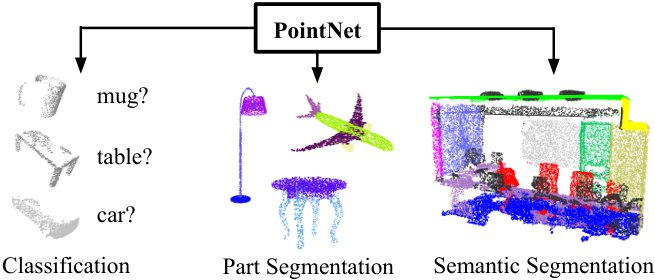
Figure 1: Applications of PointNet. We propose a novel deep net architecture that consumes raw point cloud (set of points) without voxelization or rendering. It is a unified architecture that learns both global and local point features, providing a simple, efficient and effective approach for a number of 3D recognition tasks.

图1:** PointNet的应用。 我们提出一种新颖的深网建筑,它消耗原始点云(集点)而不产生阴性或渲染. 它是一个既学习全球点又学习地方点特点的统一架构,为一些3D识别任务提供了简单、高效和有效的方法。 **

Our PointNet is a unified architecture that directly takes point clouds as input and outputs either class labels for the entire input or per point segment/part labels for each point of the input. The basic architecture of our network is surprisingly simple as in the initial stages each point is processed identically and independently. In the basic setting each point is represented by just its three coordinates $(x,y,z)$. Additional dimensions may be added by computing normals and other local or global features.

Our PointNet是一个统一的架构,它直接将点云作为输入,输出整个输入的分类标签,或者每个输入点的每个点段/部分标签. 我们网络的基本结构令人惊讶地很简单,因为在初始阶段,每个点都得到同样的和独立处理。 在基本设定中,每个点只有三个坐标$(x,y,z)$。 可以通过计算常态和其他局部或全球特征来增加额外的维度.

Key to our approach is the use of a single symmetric function, max pooling. Effectively the network learns a set of optimization functions/criteria that select interesting or informative points of the point cloud and encode the reason for their selection. The final fully connected layers of the network aggregate these learnt optimal values into the global descriptor for the entire shape as mentioned above (shape classification) or are used to predict per point labels (shape segmentation).

我们方法的关键是使用单一的对称函数,最大集合. 网络有效学习一套优化功能/标准,选择点云的有趣或信息性点,并编码其选择原因. 网络中最后的全连接层将这些获得的优化值汇总到上文提到的整个形状(形状分类)的全球描述符中,或用于预测每个点标签(形状分割)。

Our input format is easy to apply rigid or affine transformations to, as each point transforms independently. Thus we can add a data-dependent spatial transformer network that attempts to canonicalize the data before the PointNet processes them, so as to further improve the results.

我们的输入格式很容易应用刚性或亲性转换,因为每个点都独立变换. 因此,我们可以增加一个依赖数据的空间变压器网络,试图在PointNet处理之前对数据进行分类,以便进一步改善结果。

We provide both a theoretical analysis and an experimental evaluation of our approach. We show that our network can approximate any set function that is continuous. More interestingly, it turns out that our network learns to summarize an input point cloud by a sparse set of key points, which roughly corresponds to the skeleton of objects according to visualization. The theoretical analysis provides an understanding why our PointNet is highly robust to small perturbation of input points as well as to corruption through point insertion (outliers) or deletion (missing data).

我们既提供理论分析,又对我们的方法进行实验性评价。 我们显示,我们的网络可以大致 任何连续的设定函数。 更有趣的是,我们的网络 学会用稀疏的一组关键点来总结一个输入点云, 大致相当于根据可视化 物体的骨架。 理论分析提供了一种理解,绯闻为什么我们的PointNet韧性很高,小幅干扰输入点,以及通过插入点(输出点)或删除点(缺失数据)进行腐败。

On a number of benchmark datasets ranging from shape classification, part segmentation to scene segmentation, we experimentally compare our PointNet with state-of-the-art approaches based upon multi-view and volumetric representations. Under a unified architecture, not only is our PointNet much faster in speed, but it also exhibits strong performance on par or even better than state of the art.

在从形状分类,部分分割到场景分割等一系列基准数据集上,我们实验性地将我们的PointNet与基于多视图和量子表示的先进方法进行比较. 在统一的架构下,我们的PointNet的速度不仅要快得多,而且它在平面或甚至优于艺术水平上表现出强大的性能.

The key contributions of our work are as follows:

我们工作的主要贡献如下:

• • We design a novel deep net architecture suitable for consuming unordered point sets in 3D;
• • We show how such a net can be trained to perform 3D shape classification, shape part segmentation and scene semantic parsing tasks;
• • We provide thorough empirical and theoretical analysis on the stability and efficiency of our method;
• • We illustrate the 3D features computed by the selected neurons in the net and develop intuitive explanations for its performance.

• 我们设计一种适合消耗3D中无序点集的新式深网建筑;
• 我们展示如何培训这种网络,以进行三维形状分类、部分分解和场景语义解析工作;
• 就方法的稳定性和效率提供透彻的经验和理论分析;
• 我们说明由网中某些神经元计算的3D特征,并对其性能作出直观的解释。

The problem of processing unordered sets by neural nets is a very general and fundamental problem – we expect that our ideas can be transferred to other domains as well.

神经网处理无序设备的问题是一个非常普遍和根本性的问题 — — 我们期望我们的想法也能转移到其他领域。

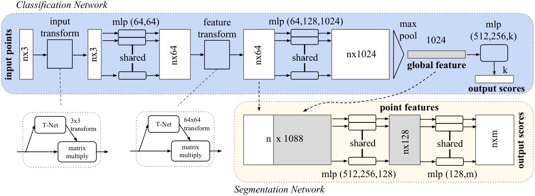
Figure 2: PointNet Architecture. The classification network takes $n$ points as input, applies input and feature transformations, and then aggregates point features by max pooling. The output is classification scores for $k$ classes. The segmentation network is an extension to the classification net. It concatenates global and local features and outputs per point scores. “mlp” stands for multi-layer perceptron, numbers in bracket are layer sizes. Batchnorm is used for all layers with ReLU. Dropout layers are used for the last mlp in classification net.

图2:**PointNet架构。 分类网络采用$n$点作为输入,应用输入和特征转换,然后通过最大集合来聚合点特征. 产出是$k$类的分类分数. 分化网是分类网的延伸. 它使全球和地方的特征和产出逐点得分均匀化。 “mlp”代表多层感官,括号中的数字是层大小。 Batchnorm用于所有带有ReLU的层. 分类网中最后一个mlp使用退学层。 **

2 Related Work

2 相关工作

Point Cloud Features

Most existing features for point cloud are handcrafted towards specific tasks. Point features often encode certain statistical properties of points and are designed to be invariant to certain transformations, which are typically classified as intrinsic [2, 24, 3] or extrinsic  [20, 19, 14, 10, 5]. They can also be categorized as local features and global features. For a specific task, it is not trivial to find the optimal feature combination.

点云特征

点云的多数现有特征都是手工完成特定任务的. 点特征常编码点的某些统计属性,并被设计成对某些变换的不常态,这些变换通常被归类为内在[2,24,3]或外在[20,19,14,10,5]. 它们也可以归类为地方特征和全球特征。 对于一项具体任务来说,找到最佳的特征组合并非微不足道。

Deep Learning on 3D Data

3D data has multiple popular representations, leading to various approaches for learning. Volumetric CNNs: [28, 17, 18] are the pioneers applying 3D convolutional neural networks on voxelized shapes. However, volumetric representation is constrained by its resolution due to data sparsity and computation cost of 3D convolution. FPNN [13] and Vote3D [26] proposed special methods to deal with the sparsity problem; however, their operations are still on sparse volumes, it’s challenging for them to process very large point clouds. Multiview CNNs: [23, 18] have tried to render 3D point cloud or shapes into 2D images and then apply 2D conv nets to classify them. With well engineered image CNNs, this line of methods have achieved dominating performance on shape classification and retrieval tasks [21]. However, it’s nontrivial to extend them to scene understanding or other 3D tasks such as point classification and shape completion. Spectral CNNs: Some latest works [4, 16] use spectral CNNs on meshes. However, these methods are currently constrained on manifold meshes such as organic objects and it’s not obvious how to extend them to non-isometric shapes such as furniture. Feature-based DNNs: [6, 8] firstly convert the 3D data into a vector, by extracting traditional shape features and then use a fully connected net to classify the shape. We think they are constrained by the representation power of the features extracted.

3D 数据的深入学习

3D数据有多种流行的表达方式,导致各种学习方法. Volumeteral CNNs: [28, 17, 18] 是应用在阴性形状上的3D进化神经网络的先驱. 然而,由于数据堆积和三维演化的计算成本,其分辨率限制了体积表示。 F抨n [13] 和 Vote3D [26] 提出了处理垃圾问题的特殊方法;然而,他们的操作量仍然很少,处理非常大的点云很困难。 多视线CNN: [23,18] 曾尝试将3D点云或形状制成2D图像,然后应用2D孔网进行分类. 有了精心设计的图像CNN,这一系列方法在形状分类和检索任务上实现了主导性能[21]. 然而,将其延伸至场景理解或其他3D任务,如点分类和形状完成,是非三角性的. 特定有线电视新闻网: 一些最新作品[4,16]在 meshes上使用光谱CNN. 然而,这些方法目前被限制在有机物等多种中间体上,而且不清楚如何将其延伸至家具等非同位素形状。 * Feature-based DNNs:* [6,8] 首先通过提取传统形状特征,将3D数据转换成矢量,然后使用全连接网对形状进行分类. 我们认为,它们受到所提取特征的代表权的限制。

Deep Learning on Unordered Sets

From a data structure point of view, a point cloud is an unordered set of vectors. While most works in deep learning focus on regular input representations like sequences (in speech and language processing), images and volumes (video or 3D data), not much work has been done in deep learning on point sets.

• 我请大家深入学习无序集

从数据结构角度来看,点云是一组无序的矢量. 虽然大部分在深度学习中注重序列(在语音和语言处理中),图像和卷(视频或3D数据)等常规输入表达,但在深度学习点集方面没有做多少工作.

One recent work from Oriol Vinyals et al [25] looks into this problem. They use a read-process-write network with attention mechanism to consume unordered input sets and show that their network has the ability to sort numbers. However, since their work focuses on generic sets and NLP applications, there lacks the role of geometry in the sets.

Oriol Vinyals等人最近的一项著作[25]研究了这一问题。 他们使用一个带有关注机制的读-进程-写网络来消耗未排序的输入集,并显示他们的网络具有排序数字的能力. 然而,由于他们的工作侧重于通用集和NLP应用,因此在集中缺乏几何作用.

3 Problem Statement

3 问题陈述

We design a deep learning framework that directly consumes unordered point sets as inputs. A point cloud is represented as a set of 3D points $\{P_{i}|\ i=1,...,n\}$, where each point $P_{i}$ is a vector of its $(x,y,z)$ coordinate plus extra feature channels such as color, normal etc. For simplicity and clarity, unless otherwise noted, we only use the $(x,y,z)$ coordinate as our point’s channels.

我们设计了一个深入的学习框架,直接消耗无序点集作为投入. 一个点云表示为一组3D点$\{P_{i}|\ i=1,...,n\}$,其中每个点$P_{i}$是其$(x,y,z)$坐标的矢量加上色彩,正常等额外的特征通道. 为了简单明了,除非另有说明,我们只使用$(x,y,z)$坐标作为我们的渠道。

For the object classification task, the input point cloud is either directly sampled from a shape or pre-segmented from a scene point cloud. Our proposed deep network outputs $k$ scores for all the $k$ candidate classes. For semantic segmentation, the input can be a single object for part region segmentation, or a sub-volume from a 3D scene for object region segmentation. Our model will output $n\times m$ scores for each of the $n$ points and each of the $m$ semantic sub-categories.

对于对象分类任务,输入点云要么直接从形状中取样,要么预先从场景点云中取样. 我们提议的深网产出$k$所有$k$候选班次的分数。 对于语义分割,输入可以是部分区域分割的单个对象,也可以是3D场景中用于物体区域分割的子卷. 我们的模型将输出$n\times m$分数为$n$分数和$m$语义子类各分数.

4 Deep Learning on Point Sets

4 点集上的深度学习

The architecture of our network (Sec 4.2) is inspired by the properties of point sets in $\mathbb{R}^{n}$ (Sec 4.1).

我们的网络架构(Sec 4.2)灵感来自$\mathbb{R}^{n}$(Sec 4.1)中的点集属性.

4.1 Properties of Point Sets in $\mathbb{R}^{n}$

4.1 $\mathbb{R}^{n}$ 中点集的性质

Our input is a subset of points from an Euclidean space. It has three main properties:

我们的输入是来自欧几利得空间的一个子集点. 它有三个主要属性:

• • Unordered. Unlike pixel arrays in images or voxel arrays in volumetric grids, point cloud is a set of points without specific order. In other words, a network that consumes $N$ 3D point sets needs to be invariant to $N!$ permutations of the input set in data feeding order.
• • Interaction among points. The points are from a space with a distance metric. It means that points are not isolated, and neighboring points form a meaningful subset. Therefore, the model needs to be able to capture local structures from nearby points, and the combinatorial interactions among local structures.
• • Invariance under transformations. As a geometric object, the learned representation of the point set should be invariant to certain transformations. For example, rotating and translating points all together should not modify the global point cloud category nor the segmentation of the points.

• 无序。 与图像中的像素阵列或体积网格中的voxel阵列不同,点云是一组没有特定顺序的点. 换句话说,一个消耗$N$ 3D点集的网络需要变异到$N!$的输入集在数据供餐顺序中的演化.
  • 各点之间的互动。 积分来自一个有距离度量的空间. 这意味着点数不是孤立的,邻位点构成一个有意义的子集. 因此,模型需要能够从附近点捕捉地方结构,以及地方结构之间的组合互动.
  · 变化中的变化。 作为一个几何物体,学得的点集的表示力应该对某些变换不具有变化性. 例如,所有旋转和翻译点不应修改全局点云类别,也不应修改点的分割。

4.2 PointNet Architecture

4.2 PointNet 架构

Our full network architecture is visualized in Fig 2, where the classification network and the segmentation network share a great portion of structures. Please read the caption of Fig 2 for the pipeline.

我们的完整 网络架构.3在图2中可视化,其中分类网络和分区网络共享了很大一部分结构. 请阅读图2的管道标题。

Our network has three key modules: the max pooling layer as a symmetric function to aggregate information from all the points, a local and global information combination structure, and two joint alignment networks that align both input points and point features.

我们的网络有三个关键模块:最大集合层作为汇总所有点信息的一个对称功能,一个局部和全球信息组合结构,以及两个既对齐输入点又对齐点特征的联合对齐网络.

We will discuss our reason behind these design choices in separate paragraphs below.

我们将在下文各段讨论这些设计选择背后的理由。

Symmetry Function for Unordered Input

In order to make a model invariant to input permutation, three strategies exist: 1) sort input into a canonical order; 2) treat the input as a sequence to train an RNN, but augment the training data by all kinds of permutations; 3) use a simple symmetric function to aggregate the information from each point. Here, a symmetric function takes $n$ vectors as input and outputs a new vector that is invariant to the input order. For example, $+$ and $*$ operators are symmetric binary functions.

未更积极地输入的对称函数

为了让模型不变量输入振荡,有三种策略:1)排序输入到犬形序列中;2)将输入作为一个序列来训练RNN,但通过各种振荡来增强训练数据;3)使用简单的对称函数来从每个点汇总信息. 在此,一个对称函数将$n$向量作为输入,输出一个新的向量,对输入顺序不具有变化性. 例如,$+$和$*$运算符都是对称的二进制函数.

While sorting sounds like a simple solution, in high dimensional space there in fact does not exist an ordering that is stable w.r.t. point perturbations in the general sense. This can be easily shown by contradiction. If such an ordering strategy exists, it defines a bijection map between a high-dimensional space and a $1d$ real line. It is not hard to see, to require an ordering to be stable w.r.t point perturbations is equivalent to requiring that this map preserves spatial proximity as the dimension reduces, a task that cannot be achieved in the general case. Therefore, sorting does not fully resolve the ordering issue, and it’s hard for a network to learn a consistent mapping from input to output as the ordering issue persists. As shown in experiments (Fig 5), we find that applying a MLP directly on the sorted point set performs poorly, though slightly better than directly processing an unsorted input.

虽然排序听起来像一个简单的解决方案,但是在高维空间中实际上并不存在一般意义上稳定w.r.t.点扰动的指令. 这很容易通过矛盾来表现. 如果这样的命令策略存在,它会定义一个高维空间和$1d$真线之间的双射图. 不难看出,要求命令是稳定的w.r.t点扰动相当于要求本地图随着维度的减少而保持空间接近,在一般情况下,这项任务是无法完成的. 因此,排序不能完全解决订单问题,随着订单问题持续存在,网络很难从投入到产出学习一致的映射. 如实验(图5)所示,我们发现在排序的点集上直接应用MLP的性能不佳,虽然略优于直接处理未排序的输入.

The idea to use RNN considers the point set as a sequential signal and hopes that by training the RNN with randomly permuted sequences, the RNN will become invariant to input order. However in “OrderMatters” [25] the authors have shown that order does matter and cannot be totally omitted. While RNN has relatively good robustness to input ordering for sequences with small length (dozens), it’s hard to scale to thousands of input elements, which is the common size for point sets. Empirically, we have also shown that model based on RNN does not perform as well as our proposed method (Fig 5).

使用RNN的想法认为定点是一个顺序信号,并希望通过随机穿透序列对RNN进行训练,RNN会变得对输入顺序无变化. 然而,在“命令材料”[25]中,提交人表明,命令确实重要,不能完全省略。 虽然RNN对于长度小(几十个)的序列的输入顺序具有相对良好的稳健性,但很难达到数千个输入元素,这是点集的常见大小. 从经验上讲,我们还表明,基于RNN的模型与我们所建议的方法(图5)相比效果不佳。

Our idea is to approximate a general function defined on a point set by applying a symmetric function on transformed elements in the set:

我们的想法是通过将一个对称的函数应用到集合中转换的元素上,来对一组点上定义的一般函数进行近似:

$$\displaystyle f(\{x_{1},\dots,x_{n}\})\approx g(h(x_{1}),\dots,h(x_{n})), \tag{1}$$

where $f:2^{\mathbb{R}^{N}}\rightarrow\mathbb{R}$, $h:\mathbb{R}^{N}\rightarrow\mathbb{R}^{K}$ and $g:\underbrace{\mathbb{R}^{K}\times\dots\times\mathbb{R}^{K}}_{n}\rightarrow\mathbb{R}$ is a symmetric function.

其中$f:2^{\mathbb{R}^{N}}\rightarrow\mathbb{R}$,$h:\mathbb{R}^{N}\rightarrow\mathbb{R}^{K}$和$g:\underbrace{\mathbb{R}^{K}\times\dots\times\mathbb{R}^{K}}_{n}\rightarrow\mathbb{R}$是一个对称函数.

Empirically, our basic module is very simple: we approximate $h$ by a multi-layer perceptron network and $g$ by a composition of a single variable function and a max pooling function. This is found to work well by experiments. Through a collection of $h$, we can learn a number of $f$’s to capture different properties of the set.

从经验上讲,我们的基本模块非常简单:我们通过多层感官网络来估计$h$,通过单个可变函数和最大集合函数组成$g$. 实验发现这效果很好。 通过$h$的集合,我们可以学习一些$f$的功能来捕捉集的不同属性.

While our key module seems simple, it has interesting properties (see Sec 5.3) and can achieve strong performace (see Sec 5.1) in a few different applications. Due to the simplicity of our module, we are also able to provide theoretical analysis as in Sec 4.3.

虽然我们的关键模块看起来很简单,但它具有有趣的属性(见Sec 5.3),可以在几个不同的应用中实现强性能(见Sec 5.1). 由于我们模块的简单,我们也能够像第4.3节那样提供理论分析。

Local and Global Information Aggregation

The output from the above section forms a vector $[f_{1},\dots,f_{K}]$, which is a global signature of the input set. We can easily train a SVM or multi-layer perceptron classifier on the shape global features for classification. However, point segmentation requires a combination of local and global knowledge. We can achieve this by a simple yet highly effective manner.

地方和全球信息汇总

上述部分的输出形成矢量$[f_{1},\dots,f_{K}]$,这是输入集的全局签名. 我们可以轻松地在形状全球特征上训练一个SVM或多层受体分类器进行分类. 然而,分点需要结合地方和全球知识。 我们可以以简单而高效的方式实现这一目标。

Our solution can be seen in Fig 2 (Segmentation Network). After computing the global point cloud feature vector, we feed it back to per point features by concatenating the global feature with each of the point features. Then we extract new per point features based on the combined point features - this time the per point feature is aware of both the local and global information.

我们的解决方案可见于图2(分区网). 在计算了全局点云特征矢量后,我们通过将全局点特征与每个点特征相配合,将其反馈回每个点的特征. 然后,我们根据综合点特征抽取每个点的新特征——这次每个点特征既了解当地信息,也了解全球信息。

With this modification our network is able to predict per point quantities that rely on both local geometry and global semantics. For example we can accurately predict per-point normals (fig in supplementary), validating that the network is able to summarize information from the point’s local neighborhood. In experiment session, we also show that our model can achieve state-of-the-art performance on shape part segmentation and scene segmentation.

通过这一修改,我们的网络能够预测每个点的数量,这些量既依赖于局部几何学,也依赖于全球语义学。 例如,我们可以精确地而被预测每个点的常态(图中为补充),验证网络能够从点的本地邻居那里总结信息. 在实验环节中,我们还显示我们的模型可以在形状部分分化和场景分化上实现最先进的性能.

Joint Alignment Network

The semantic labeling of a point cloud has to be invariant if the point cloud undergoes certain geometric transformations, such as rigid transformation. We therefore expect that the learnt representation by our point set is invariant to these transformations.

联合调整网络

点云的语义标签如果点云经过某些几何变换,如刚性变换,则必须具有不常态. 因此,我们期望,从我们的观点看,我们所学到的代表性对这些转变是无足轻重的。

A natural solution is to align all input set to a canonical space before feature extraction. Jaderberg et al. [9] introduces the idea of spatial transformer to align 2D images through sampling and interpolation, achieved by a specifically tailored layer implemented on GPU.

一个自然的解决办法是,在提取特征之前,将所有输入集与条形空间对齐。 Jaderberg et al. [9] 引入了空间变压器的想法,通过采样和插图来对齐2D图像,通过在GPU上执行的特制层实现.

Our input form of point clouds allows us to achieve this goal in a much simpler way compared with [9]. We do not need to invent any new layers and no alias is introduced as in the image case. We predict an affine transformation matrix by a mini-network (T-net in Fig 2) and directly apply this transformation to the coordinates of input points. The mini-network itself resembles the big network and is composed by basic modules of point independent feature extraction, max pooling and fully connected layers. More details about the T-net are in the supplementary.

与[9]相比,我们输入的点云形式使我们能够以简单得多的方式实现这一目标。 我们不需要发明任何新的图层,也不象图像那样引入别名。 我们通过一个小型网络(图2中的T-net)来预测一个亲缘变换矩阵,并将这种变换直接应用于输入点的坐标. 微型网络本身类似于大网络,由点独立特征提取,最大集合和全连接层等基本模块组成. 关于T网的更多详情见补充部分。

This idea can be further extended to the alignment of feature space, as well. We can insert another alignment network on point features and predict a feature transformation matrix to align features from different input point clouds. However, transformation matrix in the feature space has much higher dimension than the spatial transform matrix, which greatly increases the difficulty of optimization. We therefore add a regularization term to our softmax training loss. We constrain the feature transformation matrix to be close to orthogonal matrix:

这一想法还可以进一步扩展到特征空间的对齐. 我们可以在点状特征上插入另一个对齐网络,并预测一个特征变换矩阵,从不同的输入点云对齐特征.. . . . . 因此,我们在软最大训练损失中增加了一个正规化术语。 我们限制特征变换矩阵接近正向矩阵:

$$L_{reg}=\|I-AA^{T}\|_{F}^{2}, \tag{2}$$

where $A$ is the feature alignment matrix predicted by a mini-network. An orthogonal transformation will not lose information in the input, thus is desired. We find that by adding the regularization term, the optimization becomes more stable and our model achieves better performance.

其中$A$是小型网络预测的特征对齐矩阵. 正交转换不会在输入中丢失信息,因此是可取的. 我们发现,通过增加规范化术语,优化变得更加稳定,我们的模型实现更好的性能.

4.3 Theoretical Analysis

4.3 理论分析

Universal approximation

We first show the universal approximation ability of our neural network to continuous set functions. By the continuity of set functions, intuitively, a small perturbation to the input point set should not greatly change the function values, such as classification or segmentation scores.

通用近似值

我们首先展示我们神经网络 持续设置功能的普遍近似能力。 通过设定函数的连续性,直觉上,小扰动到输入点集不应大大改变函数值,如分类或分化分数.

Formally, let $\mathcal{X}=\{S:S\subseteq[0,1]^{m}\text{ and }|S|=n\}$, $f:\mathcal{X}\rightarrow\mathbb{R}$ is a continuous set function on $\mathcal{X}$ w.r.t to Hausdorff distance $d_{H}(\cdot,\cdot)$, i.e., $\forall\epsilon>0,\exists\delta>0$, for any $S,S^{\prime}\in\mathcal{X}$, if $d_{H}(S,S^{\prime})<\delta$, then $|f(S)-f(S^{\prime})|<\epsilon$. Our theorem says that $f$ can be arbitrarily approximated by our network given enough neurons at the max pooling layer, i.e., $K$ in (1) is sufficiently large.

形式上,让$\mathcal{X}=\{S:S\subseteq[0,1]^{m}\text{ and }|S|=n\}$,$f:\mathcal{X}\rightarrow\mathbb{R}$是$\mathcal{X}$ w.r.t到Hausdorff距离$d_{H}(\cdot,\cdot)$,即$\forall\epsilon>0,\exists\delta>0$,对任何$S,S^{\prime}\in\mathcal{X}$来说,如果$d_{H}(S,S^{\prime})<\delta$,那么$|f(S)-f(S^{\prime})|<\epsilon$是一个连续的集函数. 我们的定理说,$f$可以被我们的网络任意近似于在最大集合层给予足够的神经元,即xMATH9XX在(1)中足够大.

Theorem 1.

Suppose $f:\mathcal{X}\rightarrow\mathbb{R}$ is a continuous set function w.r.t Hausdorff distance $d_{H}(\cdot,\cdot)$. $\forall\epsilon>0$, $\exists$ a continuous function $h$ and a symmetric function $g(x_{1},\dots,x_{n})=\gamma\circ\mbox{MAX}$, such that for any $S\in\mathcal{X}$,

** 定 义 1****。 **

*Suppose XXMA例子20XX是一个连续集函数w.r.t Hausdorff 距离 $d_{H}(\cdot,\cdot)$. $\forall\epsilon>0$,$\exists$是一个连续函数$h$和一个对称函数$g(x_{1},\dots,x_{n})=\gamma\circ\mbox{MAX}$,因此对于任何$S\in\mathcal{X}$,

$$\displaystyle\left|f(S)-\gamma\left(\underset{x_{i}\in S}{\mbox{MAX}}\left\{h(x_{i})\right\}\right)\right|<\epsilon$$

where $x_{1},\ldots,x_{n}$ is the full list of elements in $S$ ordered arbitrarily, $\gamma$ is a continuous function, and MAX is a vector max operator that takes $n$ vectors as input and returns a new vector of the element-wise maximum.

• 其中XXMA 一个$x_{1},\ldots,x_{n}$是任意订购的$S$中的全部元素列表,$\gamma$是一个连续函数,MAX是一个矢量最大运算符,它以$n$矢量作为输入并返回元素最大值的新矢量. *

The proof to this theorem can be found in our supplementary material. The key idea is that in the worst case the network can learn to convert a point cloud into a volumetric representation, by partitioning the space into equal-sized voxels. In practice, however, the network learns a much smarter strategy to probe the space, as we shall see in point function visualizations.

我们的补充材料中可以找到这个定理的证据. 关键的想法是,在最坏的情况下,网络可以通过将空间分割成等大小的voxels来学习将点云转换成量子表示. 然而,实际上,网络学习了一种更聪明的探索空间的战略,我们将从点函数可视化中看到这一点。

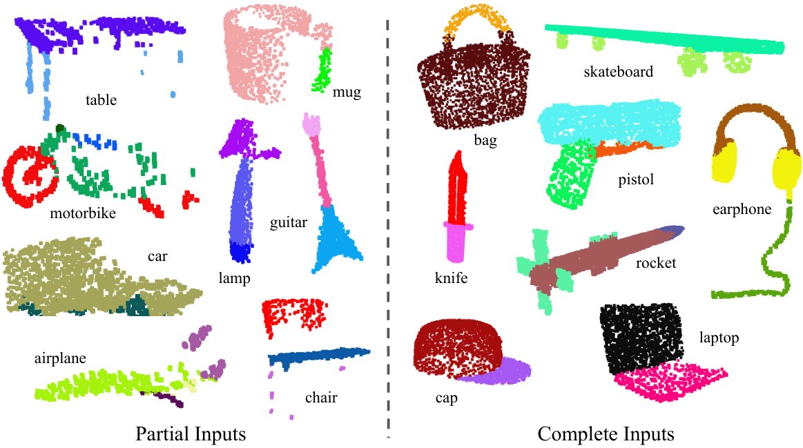
Figure 3: Qualitative results for part segmentation. We visualize the CAD part segmentation results across all 16 object categories. We show both results for partial simulated Kinect scans (left block) and complete ShapeNet CAD models (right block).

图3:部分分割的定性结果。 我们可视化CAD部分分解结果 覆盖所有16个对象类别. 我们显示部分模拟Kinect扫描(左块)的结果和完整的ShapeNet CAD模型(右块)的结果。 **

Bottleneck dimension and stability

Theoretically and experimentally we find that the expressiveness of our network is strongly affected by the dimension of the max pooling layer, i.e., $K$ in (1). Here we provide an analysis, which also reveals properties related to the stability of our model.

Bottleneck 维度和稳定性

理论上和实验上,我们发现我们的网络的表达性受到最大集合层的维度,即(1)中的$K$的强烈影响. 我们在这里提供了一种分析,它也揭示了与我们模型稳定性有关的属性。

We define $\mathbf{u}=\underset{x_{i}\in S}{\mbox{MAX}}\{h(x_{i})\}$ to be the sub-network of $f$ which maps a point set in $[0,1]^{m}$ to a $K$-dimensional vector. The following theorem tells us that small corruptions or extra noise points in the input set are not likely to change the output of our network:

我们定义$\mathbf{u}=\underset{x_{i}\in S}{\mbox{MAX}}\{h(x_{i})\}$是$f$的子网络,它将$[0,1]^{m}$中的一个点映射到$K$- 维向量. 以下定理告诉我们,输入集中小的腐败或额外的噪音点不太可能改变我们网络的输出:

Theorem 2.

Suppose $\mathbf{u}:\mathcal{X}\rightarrow\mathbb{R}^{K}$ such that $\mathbf{u}=\underset{x_{i}\in S}{\mbox{MAX}}\{h(x_{i})\}$ and $f=\gamma\circ\mathbf{u}$. Then,

• 定理2****。 **

• 补充$\mathbf{u}:\mathcal{X}\rightarrow\mathbb{R}^{K}$,使$\mathbf{u}=\underset{x_{i}\in S}{\mbox{MAX}}\{h(x_{i})\}$和$f=\gamma\circ\mathbf{u}$。

(a) $\forall S,\exists~\mathcal{C}_{S},\mathcal{N}_{S}\subseteq\mathcal{X}$,$f(T)=f(S)$if$\mathcal{C}_{S}\subseteq T\subseteq\mathcal{N}_{S}$;
(b) $|\mathcal{C}_{S}|\leq K$

(a) $\forall S,\exists~\mathcal{C}_{S},\mathcal{N}_{S}\subseteq\mathcal{X}$, $f(T)=f(S)$, $\mathcal{C}_{S}\subseteq T\subseteq\mathcal{N}_{S}$*;
(b) XIMATH3(XX)

We explain the implications of the theorem. (a) says that $f(S)$ is unchanged up to the input corruption if all points in $\mathcal{C}_{S}$ are preserved; it is also unchanged with extra noise points up to $\mathcal{N}_{S}$. (b) says that $\mathcal{C}_{S}$ only contains a bounded number of points, determined by $K$ in (1). In other words, $f(S)$ is in fact totally determined by a finite subset $\mathcal{C}_{S}\subseteq S$ of less or equal to $K$ elements. We therefore call $\mathcal{C}_{S}$ the critical point set of $S$ and $K$ the bottleneck dimension of $f$.

我们解释该定理的意义。 (a) 说如果$\mathcal{C}_{S}$中的所有点都保留的话,$f(S)$到输入腐败为止不变;它也随着到$\mathcal{N}_{S}$的额外噪点而保持不变。 (b) 说$\mathcal{C}_{S}$只在(1)中包含一个限定的点数,由$K$确定。 换句话说,$f(S)$实际上完全是由一个小于或等于$K$元素的有限子集$\mathcal{C}_{S}\subseteq S$决定的. 因此,我们称$\mathcal{C}_{S}$为$S$和$K$的临界点集为$f$的瓶颈维度。

Combined with the continuity of $h$, this explains the robustness of our model w.r.t point perturbation, corruption and extra noise points. The robustness is gained in analogy to the sparsity principle in machine learning models. Intuitively, our network learns to summarize a shape by a sparse set of key points. In experiment section we see that the key points form the skeleton of an object.

这与$h$的连续性相结合,说明了我们的模型w.r.t点扰动、腐败和额外噪音点的稳健性。 稳健性在机器学习模型中通过类比而获得,与痉挛性原则. ** 从直觉上讲,我们的网络学会用稀疏的关键点来总结一个形状。 ** 在实验部分,我们看到关键点构成物体的骨架。

5 Experiment

5 实验

	input	#views	accuracy	accuracy
			avg. class	overall
SPH [11]	mesh	-	68.2	-
3DShapeNets [28]	volume	1	77.3	84.7
VoxNet [17]	volume	12	83.0	85.9
Subvolume [18]	volume	20	86.0	89.2
LFD [28]	image	10	75.5	-
MVCNN [23]	image	80	90.1	-
Ours baseline	point	-	72.6	77.4
Ours PointNet	point	1	86.2	89.2

Table 1: Classification results on ModelNet40. Our net achieves state-of-the-art among deep nets on 3D input.

	投入	视图	准确性	准确性
			avg 类	总计
SPH [11] (英语).	网点	-	68.2	-
三维元件网 [28]	音量	1	77.3	84.7
VoxNet [17] (英语).	音量	12	83.0	85.9
分册 [18]	音量	20	86.0	页:1
LFD [28] (英语).	图像	10	75.5	-
MVCNN [23] (英语).	图像	80	页:1	-
我们的基线	点	-	72.6	77.4
我们的点网	点	1	86.2	页:1

表1:**模型Net40的分类结果。 ** 我们黏网在3D输入的深网中达到了最先进的水平。

Experiments are divided into four parts. First, we show PointNets can be applied to multiple 3D recognition tasks (Sec 5.1). Second, we provide detailed experiments to validate our network design (Sec 5.2). At last we visualize what the network learns (Sec 5.3) and analyze time and space complexity (Sec 5.4).

实验分为四部分. 首先,我们显示PointNets可以应用于多个3D识别任务(Sec 5.1. 第二,我们提供详细的实验来验证我们的网络设计(Sec 5.2)。 最后,我们可视化网络所学到的东西(第5.3节),并分析时间和空间的复杂性(第5.4节)。

	mean	aero	bag	cap	car	chair	ear	guitar	knife	lamp	laptop	motor	mug	pistol	rocket	skate	table
							phone									board
# shapes		2690	76	55	898	3758	69	787	392	1547	451	202	184	283	66	152	5271
Wu [27]	-	63.2	-	-	-	73.5	-	-	-	74.4	-	-	-	-	-	-	74.8
Yi [29]	81.4	81.0	78.4	77.7	75.7	87.6	61.9	92.0	85.4	82.5	95.7	70.6	91.9	85.9	53.1	69.8	75.3
3DCNN	79.4	75.1	72.8	73.3	70.0	87.2	63.5	88.4	79.6	74.4	93.9	58.7	91.8	76.4	51.2	65.3	77.1
Ours	83.7	83.4	78.7	82.5	74.9	89.6	73.0	91.5	85.9	80.8	95.3	65.2	93.0	81.2	57.9	72.8	80.6

Table 2: Segmentation results on ShapeNet part dataset. Metric is mIoU(%) on points. We compare with two traditional methods [27] and [29] and a 3D fully convolutional network baseline proposed by us. Our PointNet method achieved the state-of-the-art in mIoU.

	说	飞机	包装	cap	car	椅子	耳朵	吉他	刀锋	你为什么这样?	笔记本电脑	motor	纸杯	手枪	火箭	行了 为防止	页:1
							电话									董事会
形状		2690	76	55	898	3758	69	787	392	1547	451	202	184	283	66	152	5271
吴[27]	-	63.2	-	-	-	73.5	-	-	-	74.4	-	-	-	-	-	-	74.8
Yi[29]	81.4	81.0	78.4	77.7	页:1	87.6	61.9	92.0 (单位:千美元)	85.4	页:1	页:1	页:1	91.9	页:1	53.1	69.8	75.3
3个DINN	79.4	75.1	72.8	73.3	70.0	87.2	63.5	88.4	79.6	74.4	93.9	58.7	91.8	76.4	51.2	65.3	77.1
我们的	页:1	页:1	页:1	页:1	74.9	页:1	* ** 73.0 **	91.5	页:1	80.8	95.3	65.2	** 93.0 ** 中文无改动。	81.2	页:1	** 第72.8段 **	** 第80.6段**

表2:**ShapeNet部分数据集的分门别类结果。 ** 度量值在点上为mIoU(%)。 我们比较了两种传统方法[27]和[29],以及我们提出的3D全卷积网络基线. 我们的PointNet方法在mIoU实现了最先进的.

5.1 Applications

5.1 应用

In this section we show how our network can be trained to perform 3D object classification, object part segmentation and semantic scene segmentation [^1]. Even though we are working on a brand new data representation (point sets), we are able to achieve comparable or even better performance on benchmarks for several tasks.

在本节中,我们展示了如何培训我们的网络来进行3D对象分类,对象部分分割和语义场景分割[^1]. 尽管我们正在研究一种全新的数据表述方式(点集),但我们能够在几项任务的基准上取得可比甚至更好的业绩。

3D Object Classification

Our network learns global point cloud feature that can be used for object classification. We evaluate our model on the ModelNet40 [28] shape classification benchmark. There are 12,311 CAD models from 40 man-made object categories, split into 9,843 for training and 2,468 for testing. While previous methods focus on volumetric and mult-view image representations, we are the first to directly work on raw point cloud.

3D 对象分类

我们的网络学习了可用于对象分类的全局点云特征. 我们用模型Net40[28]形状分类基准来评价我们的模型。 共有12,311个CAD模型,分别来自40个人造物体类别,分为9,843个训练型和2,468个测试型. 虽然以前的方法注重于量子和穆尔特视图像的表示,但我们是第一个直接研究原始点云的.

We uniformly sample 1024 points on mesh faces according to face area and normalize them into a unit sphere. During training we augment the point cloud on-the-fly by randomly rotating the object along the up-axis and jitter the position of each points by a Gaussian noise with zero mean and 0.02 standard deviation.

我们根据面部区域对网状面孔的1024个点进行统一抽样,并将其正常化为单位球体. 在训练期间,我们用零平均值和0.02标准偏差的高斯噪声,随机旋转物体沿上轴移动,增加点云,使每个点的位置颤抖。

In Table 1, we compare our model with previous works as well as our baseline using MLP on traditional features extracted from point cloud (point density, D2, shape contour etc.). Our model achieved state-of-the-art performance among methods based on 3D input (volumetric and point cloud). With only fully connected layers and max pooling, our net gains a strong lead in inference speed and can be easily parallelized in CPU as well. There is still a small gap between our method and multi-view based method (MVCNN [23]), which we think is due to the loss of fine geometry details that can be captured by rendered images.

在表1中,我们用从点云(点密度,D2,形状轮廓等)提取的传统特征的MLP将我们的模型与以前的作品以及我们的基线进行比较。 我们的模型在基于3D输入(量子和点子云)的方法中实现了最先进的性能. 由于只有完全连接的层和最大集合,我们的网络在推论速度上获得了很强的领先性,在CPU中也很容易平行. 我们的方法和基于多视图的方法(MVCNN [23])之间还存在一个小的差距,我们认为,这是由于失去精细的几何细节,这些细节可以通过渲染的图像来捕捉.

3D Object Part Segmentation

Part segmentation is a challenging fine-grained 3D recognition task. Given a 3D scan or a mesh model, the task is to assign part category label (e.g. chair leg, cup handle) to each point or face.

QQ 3D 对象部分分割

部分分解是一项挑战性的精细的3D识别任务. 考虑到3D扫描或网格模型,任务就是为每个点或面指定部分分类标签(如椅子腿,杯柄).

We evaluate on ShapeNet part data set from [29], which contains 16,881 shapes from 16 categories, annotated with 50 parts in total. Most object categories are labeled with two to five parts. Ground truth annotations are labeled on sampled points on the shapes.

我们评价ShapeNet部分数据集来自[29],其中包含16个类别中的16 881个形状,注释中共有50个部分。 大多数对象类别都带有2至5个部分的标签. 地面真相说明在形状上的抽样点上贴上标签。

We formulate part segmentation as a per-point classification problem. Evaluation metric is mIoU on points. For each shape S of category C, to calculate the shape’s mIoU: For each part type in category C, compute IoU between groundtruth and prediction. If the union of groundtruth and prediction points is empty, then count part IoU as 1. Then we average IoUs for all part types in category C to get mIoU for that shape. To calculate mIoU for the category, we take average of mIoUs for all shapes in that category.

我们把部分分解作为每个点的分类问题。 评价衡量标准是衡量点的MIOU。 对于C类的每个形状S,计算形状的mIoU: 对于C类中的每个部分,在地面真实和预测之间计算IoU. 如果地面真实和预测点的结合是空的,那么将部分IoU算作1. 然后我们平均通过IOUs来获得C类所有部分类型的MIOU来达到这种形状. 为了计算该类的mIoU,我们对该类中的所有形状平均为mIoU.

In this section, we compare our segmentation version PointNet (a modified version of Fig 2, Segmentation Network) with two traditional methods [27] and [29] that both take advantage of point-wise geometry features and correspondences between shapes, as well as our own 3D CNN baseline. See supplementary for the detailed modifications and network architecture for the 3D CNN.

在本节中,我们比较了我们的分区版本PointNet(图2,分区网络的修改版)与两种传统方法[27]和[29],两者都利用了点位几何特征和形状之间的对应,以及我们自己的3D CNN基线. 3D CNN的详细修改和网络架构见补充.

In Table 2, we report per-category and mean IoU(%) scores. We observe a 2.3% mean IoU improvement and our net beats the baseline methods in most categories.

在表2中,我们报告每个类别和IoU(%)的得分。 我们观察到2.3%的IoU改进,我们的净额比大多数类别的基线方法要高。

	mean IoU	overall accuracy
Ours baseline	20.12	53.19
Ours PointNet	47.71	78.62

Table 3: Results on semantic segmentation in scenes. Metric is average IoU over 13 classes (structural and furniture elements plus clutter) and classification accuracy calculated on points.

	意思是木卫一	时间 , 时间 , , , , , , , , , , , , , , , , , , , , , , , , , , , , , , , , , , , , , , , , , , , , , , , , , , , , , , , , , , , , , , , , ,
我们的基线	20.12	53.19
我们的点网	** 47妍**	** 78.62 **

表3:** 场景中的语义分割结果。 ** 度量衡是平均IoU 这是个超过13个等级(结构和家具元素加杂质)和按点计算的分类精度.

	table	chair	sofa	board	mean
# instance	455	1363	55	137
Armeni et al. [1]	46.02	16.15	6.78	3.91	18.22
Ours	46.67	33.80	4.76	11.72	24.24

Table 4: Results on 3D object detection in scenes. Metric is average precision with threshold IoU 0.5 computed in 3D volumes.

	页:1	椅子	沙发	董事会	说
# 实例	455	1363	55	137
Armeni等人[1]	46.02	16.15	6.78 经常预算:	3.91	18.22
我们的	页:1	页:1	4.76	页:1	页:1

表4:** 场景中3D物体探测结果。 ** 度量衡是平均精确度,阈值IoU 0.5按3D卷计算。

We also perform experiments on simulated Kinect scans to test the robustness of these methods. For every CAD model in the ShapeNet part data set, we use Blensor Kinect Simulator [7] to generate incomplete point clouds from six random viewpoints. We train our PointNet on the complete shapes and partial scans with the same network architecture and training setting. Results show that we lose only 5.3% mean IoU. In Fig 3, we present qualitative results on both complete and partial data. One can see that though partial data is fairly challenging, our predictions are reasonable.

我们还在模拟Kinect扫描上进行实验,以测试这些方法的稳健性. 对于ShapeNet部分数据集中的每个CAD模型,我们使用Blensor Kinect模拟器[7]从六个随机角度生成不完整的点云. 我们用同样的网络架构和培训环境来训练我们的PointNet的完整形状和部分扫描. 结果显示,我们只损失5.3%,即IoU。 在图3中,我们介绍了完整和部分数据的质量结果。 人们可以看到,虽然部分数据相当具有挑战性,但我们的预测是合理的。

Semantic Segmentation in Scenes

Our network on part segmentation can be easily extended to semantic scene segmentation, where point labels become semantic object classes instead of object part labels.

• 语义分裂

我们关于部分分割的网络可以很容易地扩展至语义场景分割,即点标签成为语义对象类而不是对象部分标签.

We experiment on the Stanford 3D semantic parsing data set [1]. The dataset contains 3D scans from Matterport scanners in 6 areas including 271 rooms. Each point in the scan is annotated with one of the semantic labels from 13 categories (chair, table, floor, wall etc. plus clutter).

我们在斯坦福3D语义解析数据集进行实验[1]. 该数据集包含Matterport扫描仪在包括271个房间在内的6个区域的3D扫描. 扫描中的每一点都带有来自13类(椅子,桌子,地板,墙壁等加上杂乱无章)的语义标签之一.

To prepare training data, we firstly split points by room, and then sample rooms into blocks with area 1m by 1m. We train our segmentation version of PointNet to predict per point class in each block. Each point is represented by a 9-dim vector of XYZ, RGB and normalized location as to the room (from 0 to 1). At training time, we randomly sample 4096 points in each block on-the-fly. At test time, we test on all the points. We follow the same protocol as [1] to use k-fold strategy for train and test.

为了准备训练数据,我们首先将各点按房间划分,然后将样本室分成1m乘1m的区块. 我们训练我们的分区版 PointNet 来预测每个街区的每个点级。 每个点均以XYZ,RGB的9-dim向量为代表,并对房间进行规范定位(0-1). 在训练时间,我们随机抽取4096点 在每块飞行。 在测试时间,我们测试所有点。 我们遵循与[1]相同的协议,使用k倍策略进行列车和测试.

We compare our method with a baseline using handcrafted point features. The baseline extracts the same 9-dim local features and three additional ones: local point density, local curvature and normal. We use standard MLP as the classifier. Results are shown in Table 3, where our PointNet method significantly outperforms the baseline method. In Fig 4, we show qualitative segmentation results. Our network is able to output smooth predictions and is robust to missing points and occlusions.

我们用手工制作的点状特征来比较我们的方法和基线。 基线抽取了相同的9-dim局部特征和另外三个特征:局部点葵密度,局部曲面和正常. 我们使用标准的 MLP 作为分类器。 结果见表3,我们的PointNet方法明显超过基准方法。 在图4中,我们显示了定性分类结果。 我们的网络能够作出平稳的预测,并且能够对缺失的点和隐蔽点起到强大的作用。

Based on the semantic segmentation output from our network, we further build a 3D object detection system using connected component for object proposal (see supplementary for details). We compare with previous state-of-the-art method in Table 4. The previous method is based on a sliding shape method (with CRF post processing) with SVMs trained on local geometric features and global room context feature in voxel grids. Our method outperforms it by a large margin on the furniture categories reported.

根据我们网络的语义分解输出,我们进一步利用连接的组件构建一个3D对象检测系统,用于对象建议(详见补充). 我们与表4中以前的最先进方法进行比较。 先前的方法采用滑动形状法(采用通用报告格式后处理),对SVM进行局部几何特征和全球室内环境特征培训。 我们的方法在报告的家具类别上大大超过了它。

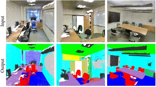
Figure 4: Qualitative results for semantic segmentation. Top row is input point cloud with color. Bottom row is output semantic segmentation result (on points) displayed in the same camera viewpoint as input.

图4:语义分割的定性结果。 上行为输入点云带色. 下行是输出语义分区结果(在点上),显示在与输入相同的相机角度。 **

5.2 Architecture Design Analysis

5.2 架构设计分析

In this section we validate our design choices by control experiments. We also show the effects of our network’s hyperparameters.

本节通过控制实验验证我们的设计选择。 我们还展示了我们网络的超参数的影响。

Comparison with Alternative Order-invariant Methods

As mentioned in Sec 4.2, there are at least three options for consuming unordered set inputs. We use the ModelNet40 shape classification problem as a test bed for comparisons of those options, the following two control experiment will also use this task.

• 与备选顺序变量方法的比较

如Sec 4.2所述,消费未经订购的成套投入至少有三种选择。 我们使用ModelNet40形状分类问题作为比较这些选项的试验床,接下来的两个控制实验也将使用这项任务.

The baselines (illustrated in Fig 5) we compared with include multi-layer perceptron on unsorted and sorted points as $n\times 3$ arrays, RNN model that considers input point as a sequence, and a model based on symmetry functions. The symmetry operation we experimented include max pooling, average pooling and an attention based weighted sum. The attention method is similar to that in [25], where a scalar score is predicted from each point feature, then the score is normalized across points by computing a softmax. The weighted sum is then computed on the normalized scores and the point features. As shown in Fig 5, max-pooling operation achieves the best performance by a large winning margin, which validates our choice.

与我们比较的基线(在图5中被忽略)包括:作为$n\times 3$阵列的无排序点上的多层受体,将输入点视为序列的RNN模型,以及基于对称函数的模型. 我们试验的对称操作包括最大集合,平均集合和基于注意力的加权总和. 注意方法与[25]中相似,其中从每个点的特征预测一个scalar分数,然后通过计算一个软max使分数在点数之间正常化. 然后,加权和数按正常的分数和点数特征计算。 如图5所示,最大集合操作以大胜率实现最佳表现,这证实了我们的选择.

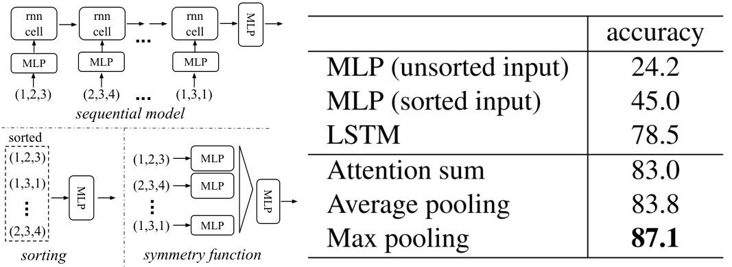
Figure 5: Three approaches to achieve order invariance. Multi-layer perceptron (MLP) applied on points consists of 5 hidden layers with neuron sizes 64,64,64,128,1024, all points share a single copy of MLP. The MLP close to the output consists of two layers with sizes 512,256.

图5:实现顺序变化的三种办法。 应用在点上的多层受体(MLP)由5个隐藏层组成,神经元尺寸为64,64,64,128,1024,所有点都共享一个MLP的单拷贝. 接近输出的MLP由两层组成,尺寸为512,256..

Effectiveness of Input and Feature Transformations

In Table 5 we demonstrate the positive effects of our input and feature transformations (for alignment). It’s interesting to see that the most basic architecture already achieves quite reasonable results. Using input transformation gives a $0.8\%$ performance boost. The regularization loss is necessary for the higher dimension transform to work. By combining both transformations and the regularization term, we achieve the best performance.

投入和特性转化的有效性

在表5中,我们展示了我们的投入和特征转变的积极影响(为调整)。 有趣的是,最基本的建筑已经取得了相当合理的效果。 使用输入转换使$0.8\%$性能提升. 正规化的丧失对于更高的层面转变为工作是必要的。 通过将转型和正规化这两个术语结合起来,我们取得了最佳业绩。

Transform	accuracy
none	87.1
input (3x3)	87.9
feature (64x64)	86.9
feature (64x64) + reg.	87.4
both	89.2

Table 5: Effects of input feature transforms. Metric is overall classification accuracy on ModelNet40 test set.

变形	准确性
无	87.1
unit( 3x3) 输入	87.9
特性( 64x64)	86.9
特性 (64x64) + reg.	87.4
两者	页:1

表5:**输入特性的影响变化。 ** Metric是ModelNet40测试集上的整体分类精度.

Robustness Test

We show our PointNet, while simple and effective, is robust to various kinds of input corruptions. We use the same architecture as in Fig 5’s max pooling network. Input points are normalized into a unit sphere. Results are in Fig 6.

强性测试

我们的PointNet虽然简单有效, 我们使用与图5最大集合网络相同的架构。 输入点被正常化为单位球体。 结果见图6。

As to missing points, when there are $50\%$ points missing, the accuracy only drops by $2.4\%$ and $3.8\%$ w.r.t. furthest and random input sampling. Our net is also robust to outlier points, if it has seen those during training. We evaluate two models: one trained on points with $(x,y,z)$ coordinates; the other on $(x,y,z)$ plus point density. The net has more than $80\%$ accuracy even when $20\%$ of the points are outliers. Fig 6 right shows the net is robust to point perturbations.

至于缺失点,当缺少XXMATH 让我们看到$50\%$点时,精确度只下降$2.4\%$和$3.8\%$ w.r.t.最远和随机输入抽样. 我们的网络如果在训练期间看到过的话,也会强大到超越点。 我们评价两种模式:一种是在使用$(x,y,z)$坐标点上训练的;另一种是在$(x,y,z)$加点密度上训练的。 网点即使有$20\%$点外值,其精度也超过$80\%$. 右图6显示网状强力指点扰动.

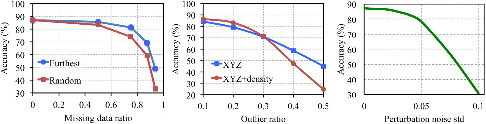
Figure 6: PointNet robustness test. The metric is overall classification accuracy on ModelNet40 test set. Left: Delete points. Furthest means the original 1024 points are sampled with furthest sampling. Middle: Insertion. Outliers uniformly scattered in the unit sphere. Right: Perturbation. Add Gaussian noise to each point independently.

图6:**PointNet稳健性测试。 衡量标准是ModelNet40测试集的整体分类精度. 左边:删除点。 Furthest表示原1024点的采样方式为最远的采样. 中间:插入. 统一分布在单位球体内。 对曰:扰. 将高斯噪音独立添加到每个点。 **

5.3 Visualizing PointNet

5.3 可视化 PointNet

In Fig 7, we visualize critical point sets $\mathcal{C}_{S}$ and upper-bound shapes $\mathcal{N}_{S}$ (as discussed in Thm 2) for some sample shapes $S$. The point sets between the two shapes will give exactly the same global shape feature $f(S)$.

在图7中,我们可视化一些样本形状的*临界点集 *$\mathcal{C}_{S}$和 * 上行形状 * $\mathcal{N}_{S}$(如Thm 2所述)。 两个形状之间的点集将给出完全相同的全球形状特征$f(S)$.

We can see clearly from Fig 7 that the critical point sets $\mathcal{C}_{S}$, those contributed to the max pooled feature, summarizes the skeleton of the shape. The upper-bound shapes $\mathcal{N}_{S}$ illustrates the largest possible point cloud that give the same global shape feature $f(S)$ as the input point cloud $S$. $\mathcal{C}_{S}$ and $\mathcal{N}_{S}$ reflect the robustness of PointNet, meaning that losing some non-critical points does not change the global shape signature $f(S)$ at all.

我们从图7中可以清楚地看到,“临界点集”$\mathcal{C}_{S}$是对最大集合特性的贡献,概括了形状的骨架。 *上行形状 *$\mathcal{N}_{S}$ 显示最大点云,给出与输入点云 $S$相同的全球形状特征$f(S)$。 $\mathcal{C}_{S}$和$\mathcal{N}_{S}$反映了PointNet的稳健性,意思是失去一些非临界点完全不会改变全球形状的签名$f(S)$.

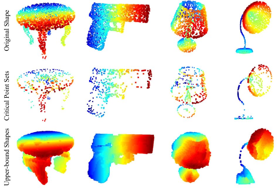
Figure 7: Critical points and upper bound shape. While critical points jointly determine the global shape feature for a given shape, any point cloud that falls between the critical points set and the upper bound shape gives exactly the same feature. We color-code all figures to show the depth information.

图7:** 临界点和上界形状。 虽然临界点共同决定了给定形状的全局形状特征,但是在临界点集和上方约束形状之间掉落的任何点云都给出了完全相同的特征. 我们用颜色编码所有数字来显示深度信息。 **

The $\mathcal{N}_{S}$ is constructed by forwarding all the points in a edge-length-2 cube through the network and select points $p$ whose point function values $(h_{1}(p),h_{2}(p),\cdots,h_{K}(p))$ are no larger than the global shape descriptor.

$\mathcal{N}_{S}$是通过网络将边缘长度-2立方体中的所有点数转发到并选择点数$p$,其点数值$(h_{1}(p),h_{2}(p),\cdots,h_{K}(p))$不大于全局形状描述符.

5.4 Time and Space Complexity Analysis

5.4 时间与空间复杂度分析

Table 6 summarizes space (number of parameters in the network) and time (floating-point operations/sample) complexity of our classification PointNet. We also compare PointNet to a representative set of volumetric and multi-view based architectures in previous works.

表6概述了我们分类点网的空间(网络参数数)和时间(浮动点操作/抽样)复杂性。 我们还将PointNet比作前几部作品中具有代表性的一套以卷式和多视图为基础的架构.

While MVCNN [23] and Subvolume (3D CNN)  [18] achieve high performance, PointNet is orders more efficient in computational cost (measured in FLOPs/sample: 141x and 8x more efficient, respectively). Besides, PointNet is much more space efficient than MVCNN in terms of #param in the network (17x less parameters). Moreover, PointNet is much more scalable – it’s space and time complexity is $O(N)$ – linear in the number of input points. However, since convolution dominates computing time, multi-view method’s time complexity grows squarely on image resolution and volumetric convolution based method grows cubically with the volume size.

虽然MVCNN [23] 和Sub 也许量(3D CNN) [18] 实现高性能,但PointNet则是在计算成本方面效率更高的订单(分别以FLOPs/样本衡量:141x和8x). 此外,PointNet在网络中的#param(17x减参数)方面比MVCNN高效得多. 此外,PointNet更具有伸缩性 — — 它的空间和时间复杂性是$O(N)$ — — 输入点数中的线性*. 然而,由于convolution主导了计算时间,多视图方法的时间复杂性在图像分辨率上“平均地”增长,而基于量子的Comvolution方法随着体积大小而增长。

Empirically, PointNet is able to process more than one million points per second for point cloud classification (around 1K objects/second) or semantic segmentation (around 2 rooms/second) with a 1080X GPU on TensorFlow, showing great potential for real-time applications.

从经验上讲,PointNet能够每秒处理超过100万个点,用于点云分类(约1K对象/秒)或语义分区(约2个房间/秒),在TensorFlow上装有1080XGPU,显示出巨大的实时应用潜力.

	#params	FLOPs/sample
PointNet (vanilla)	0.8M	148M
PointNet	3.5M	440M
Subvolume [18]	16.6M	3633M
MVCNN [23]	60.0M	62057M

Table 6: Time and space complexity of deep architectures for 3D data classification. PointNet (vanilla) is the classification PointNet without input and feature transformations. FLOP stands for floating-point operation. The “M” stands for million. Subvolume and MVCNN used pooling on input data from multiple rotations or views, without which they have much inferior performance.

	#params	FLOPs/样本
点网(香草)	0.8M (中文(简体) ).	148M (英语).
点网	3.5M (韩语)	440 就在这时
魄力(18)	16.6百万辆	3633M (英语).
MVCNN [23] (英语).	60 000万美元	62057M (英语).

表6:**3D数据分类深层架构的时间和空间复杂性. PointNet(vanilla)是分类的PointNet,没有输入和特征转换. FLOP代表着浮点操作. “M”代表百万。 分卷和MVCNN使用从多个旋转或视图中汇集输入数据,没有这些数据,其性能就低得多。 **

6 Conclusion

6 结论

In this work, we propose a novel deep neural network PointNet that directly consumes point cloud. Our network provides a unified approach to a number of 3D recognition tasks including object classification, part segmentation and semantic segmentation, while obtaining on par or better results than state of the arts on standard benchmarks. We also provide theoretical analysis and visualizations towards understanding of our network.

在这部作品中,我们提出一个新的深层神经网络PointNet直接消耗点云. 我们的网络为一些三维识别斤计较的任务提供了统一的方法,包括对象分类,部分分化和语义分化,同时在标准基准上取得与艺术状态相比的同等或更好的结果. 我们还提供理论分析和视觉,以了解我们的网络。

Acknowledgement.

The authors gratefully acknowledge the support of a Samsung GRO grant, ONR MURI N00014-13-1-0341 grant, NSF grant IIS-1528025, a Google Focused Research Award, a gift from the Adobe corporation and hardware donations by NVIDIA.

感谢。

提交人 你好地感谢三星GRO赠款、ONR MURI N00014-13-1-0341赠款、NSF赠款IS-1528025、Google焦点研究奖、Adobe公司的礼物和NVIDIA的硬件捐赠。

References

参考文献

[1] I. Armeni, O. Sener, A. R. Zamir, H. Jiang, I. Brilakis, M. Fischer, and S. Savarese. 3d semantic parsing of large-scale indoor spaces. In Proceedings of the IEEE International Conference on Computer Vision and Pattern Recognition , 2016.

[2] M. Aubry, U. Schlickewei, and D. Cremers. The wave kernel signature: A quantum mechanical approach to shape analysis. In Computer Vision Workshops (ICCV Workshops), 2011 IEEE International Conference on , pages 1626–1633. IEEE, 2011.

[3] M. M. Bronstein and I. Kokkinos. Scale-invariant heat kernel signatures for non-rigid shape recognition. In Computer Vision and Pattern Recognition (CVPR), 2010 IEEE Conference on , pages 1704–1711. IEEE, 2010.

[4] J. Bruna, W. Zaremba, A. Szlam, and Y. LeCun. Spectral networks and locally connected networks on graphs. arXiv preprint arXiv:1312.6203 , 2013.

[5] D.-Y. Chen, X.-P. Tian, Y.-T. Shen, and M. Ouhyoung. On visual similarity based 3d model retrieval. In Computer graphics forum , volume 22, pages 223–232. Wiley Online Library, 2003.

[6] Y. Fang, J. Xie, G. Dai, M. Wang, F. Zhu, T. Xu, and E. Wong. 3d deep shape descriptor. In Proceedings of the IEEE Conference on Computer Vision and Pattern Recognition , pages 2319–2328, 2015.

[7] M. Gschwandtner, R. Kwitt, A. Uhl, and W. Pree. BlenSor: Blender Sensor Simulation Toolbox Advances in Visual Computing. volume 6939 of Lecture Notes in Computer Science , chapter 20, pages 199–208. Springer Berlin / Heidelberg, Berlin, Heidelberg, 2011.

[8] K. Guo, D. Zou, and X. Chen. 3d mesh labeling via deep convolutional neural networks. ACM Transactions on Graphics (TOG) , 35(1):3, 2015.

[9] M. Jaderberg, K. Simonyan, A. Zisserman, et al. Spatial transformer networks. In NIPS 2015 .

[10] A. E. Johnson and M. Hebert. Using spin images for efficient object recognition in cluttered 3d scenes. IEEE Transactions on pattern analysis and machine intelligence , 21(5):433–449, 1999.

[11] M. Kazhdan, T. Funkhouser, and S. Rusinkiewicz. Rotation invariant spherical harmonic representation of 3 d shape descriptors. In Symposium on geometry processing , volume 6, pages 156–164, 2003.

[12] Y. LeCun, L. Bottou, Y. Bengio, and P. Haffner. Gradient-based learning applied to document recognition. Proceedings of the IEEE , 86(11):2278–2324, 1998.

[13] Y. Li, S. Pirk, H. Su, C. R. Qi, and L. J. Guibas. Fpnn: Field probing neural networks for 3d data. arXiv preprint arXiv:1605.06240 , 2016.

[14] H. Ling and D. W. Jacobs. Shape classification using the inner-distance. IEEE transactions on pattern analysis and machine intelligence , 29(2):286–299, 2007.

[15] L. v. d. Maaten and G. Hinton. Visualizing data using t-sne. Journal of Machine Learning Research , 9(Nov):2579–2605, 2008.

[16] J. Masci, D. Boscaini, M. Bronstein, and P. Vandergheynst. Geodesic convolutional neural networks on riemannian manifolds. In Proceedings of the IEEE International Conference on Computer Vision Workshops , pages 37–45, 2015.

[17] D. Maturana and S. Scherer. Voxnet: A 3d convolutional neural network for real-time object recognition. In IEEE/RSJ International Conference on Intelligent Robots and Systems , September 2015.

[18] C. R. Qi, H. Su, M. Nießner, A. Dai, M. Yan, and L. Guibas. Volumetric and multi-view cnns for object classification on 3d data. In Proc. Computer Vision and Pattern Recognition (CVPR), IEEE , 2016.

[19] R. B. Rusu, N. Blodow, and M. Beetz. Fast point feature histograms (fpfh) for 3d registration. In Robotics and Automation, 2009. ICRA’09. IEEE International Conference on , pages 3212–3217. IEEE, 2009.

[20] R. B. Rusu, N. Blodow, Z. C. Marton, and M. Beetz. Aligning point cloud views using persistent feature histograms. In 2008 IEEE/RSJ International Conference on Intelligent Robots and Systems , pages 3384–3391. IEEE, 2008.

[21] M. Savva, F. Yu, H. Su, M. Aono, B. Chen, D. Cohen-Or, W. Deng, H. Su, S. Bai, X. Bai, et al. Shrec’16 track large-scale 3d shape retrieval from shapenet core55.

[22] P. Y. Simard, D. Steinkraus, and J. C. Platt. Best practices for convolutional neural networks applied to visual document analysis. In ICDAR , volume 3, pages 958–962, 2003.

[23] H. Su, S. Maji, E. Kalogerakis, and E. G. Learned-Miller. Multi-view convolutional neural networks for 3d shape recognition. In Proc. ICCV, to appear , 2015.

[24] J. Sun, M. Ovsjanikov, and L. Guibas. A concise and provably informative multi-scale signature based on heat diffusion. In Computer graphics forum , volume 28, pages 1383–1392. Wiley Online Library, 2009.

[25] O. Vinyals, S. Bengio, and M. Kudlur. Order matters: Sequence to sequence for sets. arXiv preprint arXiv:1511.06391 , 2015.

[26] D. Z. Wang and I. Posner. Voting for voting in online point cloud object detection. Proceedings of the Robotics: Science and Systems, Rome, Italy , 1317, 2015.

[27] Z. Wu, R. Shou, Y. Wang, and X. Liu. Interactive shape co-segmentation via label propagation. Computers & Graphics , 38:248–254, 2014.

[28] Z. Wu, S. Song, A. Khosla, F. Yu, L. Zhang, X. Tang, and J. Xiao. 3d shapenets: A deep representation for volumetric shapes. In Proceedings of the IEEE Conference on Computer Vision and Pattern Recognition , pages 1912–1920, 2015.

[29] L. Yi, V. G. Kim, D. Ceylan, I.-C. Shen, M. Yan, H. Su, C. Lu, Q. Huang, A. Sheffer, and L. Guibas. A scalable active framework for region annotation in 3d shape collections. SIGGRAPH Asia , 2016.

Supplementary

补充材料

Appendix A Overview

附录 A 概述

This document provides additional quantitative results, technical details and more qualitative test examples to the main paper.

本文件为主要论文提供了更多的量化结果、技术细节和更多的质量测试实例。

In Sec B we extend the robustness test to compare PointNet with VoxNet on incomplete input. In Sec C we provide more details on neural network architectures, training parameters and in Sec D we describe our detection pipeline in scenes. Then Sec E illustrates more applications of PointNet, while Sec F shows more analysis experiments. Sec G provides a proof for our theory on PointNet. At last, we show more visualization results in Sec H.

在Sec B中,我们扩展了强性测试,将PointNet和VoxNet在不完整输入上进行比较. 在Sec C中,我们提供了更多关于神经网络架构,训练参数的细节,在Sec D中,我们描述了我们在场景中的检测管道. 随后Sec E演示了更多PointNet的应用,而Sec F演示了更多分析实验. Sec G为我们在PointNet上的理论提供了证据. 终于,我们在Sec H中显示出更多的视觉效果.

Appendix B Comparison between PointNet and VoxNet (Sec 5.2)

附录 B PointNet 与 VoxNet 的对比（第 5.2 节）

We extend the experiments in Sec 5.2 Robustness Test to compare PointNet and VoxNet [17] (a representative architecture for volumetric representation) on robustness to missing data in the input point cloud. Both networks are trained on the same train test split with 1024 number of points as input. For VoxNet we voxelize the point cloud to $32\times 32\times 32$ occupancy grids and augment the training data by random rotation around up-axis and jittering.

我们扩展了Sec 5.2强力测试中的实验,以比较PointNet和VoxNet17关于强力的实验到输入点云中缺失的数据. 两个网络都接受相同的列车测试分解训练,输入点数为1024个. 对VoxNet来说,我们把点云转换成$32\times 32\times 32$占用网格,并通过绕上轴和振动来增加训练数据。

At test time, input points are randomly dropped out by a certain ratio. As VoxNet is sensitive to rotations, its prediction uses average scores from 12 viewpoints of a point cloud. As shown in Fig 8, we see that our PointNet is much more robust to missing points. VoxNet’s accuracy dramatically drops when half of the input points are missing, from $86.3\%$ to $46.0\%$ with a $40.3\%$ difference, while our PointNet only has a $3.7\%$ performance drop. This can be explained by the theoretical analysis and explanation of our PointNet – it is learning to use a collection of critical points to summarize the shape, thus it is very robust to missing data.

在测试时间,输入点被随机地以一定的比例淘汰. 由于VoxNet对旋转很敏感,因此其预测使用点云的12个角度的平均分数. 如图8所示,我们看到,我们的PointNet对缺失点来说要强得多。 VoxNet的精度在一半输入点缺失时急剧下降,从$86.3\%$到$46.0\%$有$40.3\%$的差数,而我们的PointNet只有$3.7\%$的性能下降. 我们的PointNet(PointNet)的理论分析和解释可以解释这一点,它正在学习用一个“关键点* ” 的集合来总结形状,因此它非常强健地缺少数据。

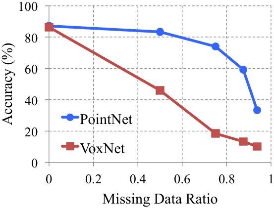
Figure 8: PointNet v.s. VoxNet [17] on incomplete input data. Metric is overall classification accurcacy on ModelNet40 test set. Note that VoxNet is using 12 viewpoints averaging while PointNet is using only one view of the point cloud. Evidently PointNet presents much stronger robustness to missing points.

图8:**PointNet v.s. VoxNet [17] 关于不完整的输入数据。 Metric是ModelNet40测试集上的整体分类精确度. 注意VoxNet使用12个平均视角,而PointNet只使用一个点云视图. 显然,PointNet对缺失点的强度要强得多。 **

Appendix C Network Architecture and Training Details (Sec 5.1)

附录 C 网络架构与训练细节（第 5.1 节）

PointNet Classification Network

As the basic architecture is already illustrated in the main paper, here we provides more details on the joint alignment/transformation network and training parameters.

点网分类网络

主要文件已经说明了基本架构,在此我们提供了联合调整/转换网络和培训参数的更多细节。

The first transformation network is a mini-PointNet that takes raw point cloud as input and regresses to a $3\times 3$ matrix. It’s composed of a shared $MLP(64,128,1024)$ network (with layer output sizes 64, 128, 1024) on each point, a max pooling across points and two fully connected layers with output sizes $512$, $256$. The output matrix is initialized as an identity matrix. All layers, except the last one, include ReLU and batch normalization. The second transformation network has the same architecture as the first one except that the output is a $64\times 64$ matrix. The matrix is also initialized as an identity. A regularization loss (with weight 0.001) is added to the softmax classification loss to make the matrix close to orthogonal.

第一个变换网络是一个小型PointNet,将原始点云作为输入,并递归到$3\times 3$矩阵. 它由一个共享的$MLP(64,128,1024)$网络(每点的层输出大小为64,128,1024)组成,一个最大跨点集合,两个完全连接的层输出大小为$512$,$256$. 输出矩阵作为身份矩阵初始化. 除最后一层外,所有层都包括ReLU和批归一化. 第二个变换网络的架构与第一个相同,只是输出是$64\times 64$矩阵. 矩阵也被初始化为身份. 在软马克思分类损失中加入一个正态损失(带有重量0.001),使基质接近正交.

We use dropout with keep ratio $0.7$ on the last fully connected layer, whose output dimension $256$, before class score prediction. The decay rate for batch normalization starts with $0.5$ and is gradually increased to $0.99$. We use adam optimizer with initial learning rate $0.001$, momentum $0.9$ and batch size $32$. The learning rate is divided by 2 every 20 epochs. Training on ModelNet takes 3-6 hours to converge with TensorFlow and a GTX1080 GPU.

在排行榜预测前,我们使用排行榜,将$0.7$比率保持在完全连接的最后一个层,其输出维度为$256$。 批归一化的衰减率从$0.5$开始,并逐渐提高到$0.99$. 我们使用具有初始学习率$0.001$,动力$0.9$和批量大小$32$的Adam优化器. 学习率除以每20个世纪2个. 关于ModelNet的培训需要3-6小时才能与TensorFlow和一个GTX1080GPU汇合.

PointNet Segmentation Network

The segmentation network is an extension to the classification PointNet. Local point features (the output after the second transformation network) and global feature (output of the max pooling) are concatenated for each point. No dropout is used for segmentation network. Training parameters are the same as the classification network.

点网分块网络

分区网是分类点网的延伸. 局部点特性(第二个变换网络后的输出)和全局特性(最大集合的输出)为每个点的缩写. 分区网络不使用退出。 训练参数与分类网相同.

As to the task of shape part segmentation, we made a few modifications to the basic segmentation network architecture (Fig 2 in main paper) in order to achieve best performance, as illustrated in Fig 9. We add a one-hot vector indicating the class of the input and concatenate it with the max pooling layer’s output. We also increase neurons in some layers and add skip links to collect local point features in different layers and concatenate them to form point feature input to the segmentation network.

关于形状碧部分分化的任务,我们对基本的碧部分网络架构(正文图2)做了几处修改,以达到最佳的性能,如图9所示. 我们添加一个一热矢量,表示输入的类别,并将其与最大集合层的输出相配合。 我们还在某些层中增加神经元,并加入跳过链接,以收集不同层的局部点特征,并将其凝结,形成点特征输入到分区网络中.

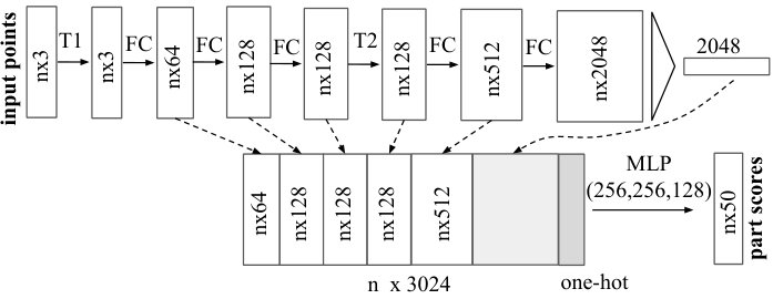
Figure 9: Network architecture for part segmentation. T1 and T2 are alignment/transformation networks for input points and features. FC is fully connected layer operating on each point. MLP is multi-layer perceptron on each point. One-hot is a vector of size 16 indicating category of the input shape.

图9:** 部分分割的网络架构。 T1和T2是用于输入点和特性的对齐/转换网络. FC是每个点上运行的全连接层. MLP在每个点上都是多层的受体. đó是16个大小的矢量,表示输入形状的类别。 **

While [27] and [29] deal with each object category independently, due to the lack of training data for some categories (the total number of shapes for all the categories in the data set are shown in the first line), we train our PointNet across categories (but with one-hot vector input to indicate category). To allow fair comparison, when testing these two models, we only predict part labels for the given specific object category.

虽然[27]和[29]分别独立处理每个对象类别,但由于某些类别缺乏训练数据(数据集中所有类别的形状总数在第一行显示),但我们将我们的PointNet进行跨类别的训练(但使用一热矢量输入表示类别). 为了进行公平的比较,在测试这两个模型时,我们只预测特定对象类别的部分标签.

As to semantic segmentation task, we used the architecture as in Fig 2 in the main paper.

至于语义分解任务,我们像主要论文的图2一样使用了架构.

It takes around six to twelve hours to train the model on ShapeNet part dataset and around half a day to train on the Stanford semantic parsing dataset.

在ShapeNet部分数据集上训练模型大约需要六到十二小时,在斯坦福语义解析数据集上训练大约需要半天时间.

Baseline 3D CNN Segmentation Network

In ShapeNet part segmentation experiment, we compare our proposed segmentation version PointNet to two traditional methods as well as a 3D volumetric CNN network baseline. In Fig 10, we show the baseline 3D volumetric CNN network we use. We generalize the well-known 3D CNN architectures, such as VoxNet [17] and 3DShapeNets [28] to a fully convolutional 3D CNN segmentation network.

基线 3D CNN 分区网络

在ShapeNet部分分区试验中,我们将我们提议的分区版本PointNet与两种传统方法以及3D卷式CNN网络基线进行比较。 在图10中,我们显示我们使用的基线3D卷式CNN网络。 我们把著名的3D CNN架构,如VoxNet [17] 和3D ShapeNets [28] 概括到一个完全革命性的3D CNN分区网络.

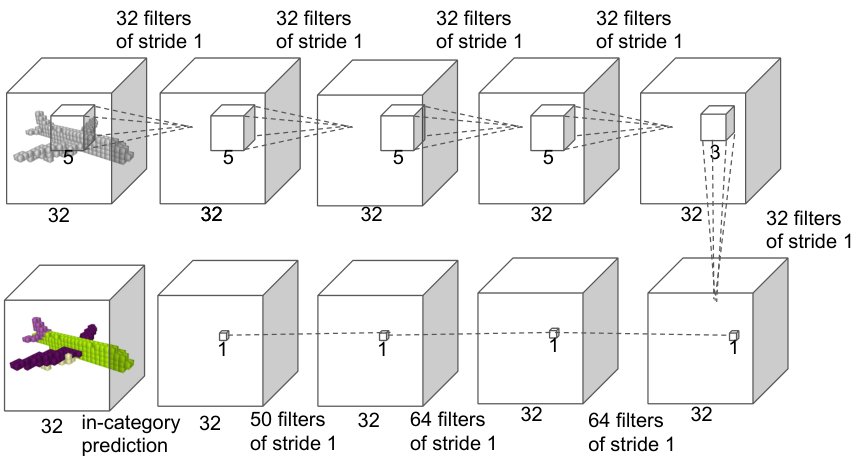
Figure 10: Baseline 3D CNN segmentation network. The network is fully convolutional and predicts part scores for each voxel.

图10:**Baseline 3D CNN分区网络. 网络是完全演化的,并预测每个阴道的部分分抨。 **

For a given point cloud, we first convert it to the volumetric representation as a occupancy grid with resolution $32\times 32\times 32$. Then, five 3D convolution operations each with 32 output channels and stride of 1 are sequentially applied to extract features. The receptive field is 19 for each voxel. Finally, a sequence of 3D convolutional layers with kernel size $1\times 1\times 1$ is appended to the computed feature map to predict segmentation label for each voxel. ReLU and batch normalization are used for all layers except the last one. The network is trained across categories, however, in order to compare with other baseline methods where object category is given, we only consider output scores in the given object category.

对于某一点云,我们首先用$32\times 32\times 32$号决议将它转换成容量表示网格。 然后,将5个3D的演化操作各带32个输出通道和1的步法相继应用来提取特性. 接受球场每瓶19分 最后,一个带有内核大小$1\times 1\times 1$的3D演化层的序列附在计算出的特征图上,以预测每个阴道的分化标签. 除最后一层外,所有层都采用ReLU和批归一化。 然而,网络经过不同类别的培训,为了与给出对象类别的其他基准方法进行比较,我们只考虑特定对象类别的输出分数.

Appendix D Details on Detection Pipeline (Sec 5.1)

附录 D 检测流程细节（第 5.1 节）

We build a simple 3D object detection system based on the semantic segmentation results and our object classification PointNet.

我们基于语义分解结果 和我们的目标分类点网 构建了一个简单的3D物体检测系统

We use connected component with segmentation scores to get object proposals in scenes. Starting from a random point in the scene, we find its predicted label and use BFS to search nearby points with the same label, with a search radius of $0.2$ meter. If the resulted cluster has more than 200 points (assuming a 4096 point sample in a 1m by 1m area), the cluster’s bounding box is marked as one object proposal. For each proposed object, it’s detection score is computed as the average point score for that category. Before evaluation, proposals with extremely small areas/volumes are pruned. For tables, chairs and sofas, the bounding boxes are extended to the floor in case the legs are separated with the seat/surface.

我们使用带分数的连接组件在场景中获取对象建议. 从场景的随机点开始,我们发现其预测的标签,并使用BFS搜索带有相同标签的附近点,搜索半径为$0.2$米. 如果结果的集群有超过200个点(假设1米乘1米面积的4096个点样本),则集群的定界框被标记为一个对象建议. 对于每个拟议对象,检测分数作为该类别的平均分数计算。 在评价前,对面积/量极小的提案进行审查。 对于桌子,椅子和沙发,边框被延伸至地板,以防腿与座椅/表面分开.

We observe that in some rooms such as auditoriums lots of objects (e.g. chairs) are close to each other, where connected component would fail to correctly segment out individual ones. Therefore we leverage our classification network and uses sliding shape method to alleviate the problem for the chair class. We train a binary classification network for each category and use the classifier for sliding window detection. The resulted boxes are pruned by non-maximum suppression. The proposed boxes from connected component and sliding shapes are combined for final evaluation.

我们看到,在一些房间,如礼堂,许多物体(如椅子)相互接近,在这些房间里,连接的部件无法正确分割单个物体。 因此,我们利用我们的分类网络,使用滑动形状方法来缓解椅子班的问题。 我们为每个类别培训一个二进制分类网络,并使用分类器进行滑动窗口检测. 爸妈,结果的盒子被非最大程度的压制 爸·沃伦(签名)

In Fig 11, we show the precision-recall curves for object detection. We trained six models, where each one of them is trained on five areas and tested on the left area. At test phase, each model is tested on the area it has never seen. The test results for all six areas are aggregated for the PR curve generation.

在图11中,我们显示用于物体探测的精度-召回曲线. 我们训练了6个模型,其中每个模型都接受五个领域的训练,并在左边区域进行测试。 在测试阶段,每个型号都在其从未见过的地区进行测试. 所有六个领域的测试结果都汇总为PR曲线生成.

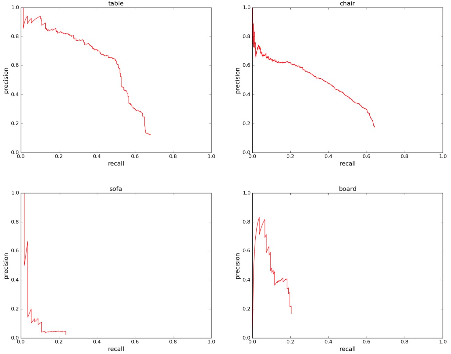
Figure 11: Precision-recall curves for object detection in 3D point cloud. We evaluated on all six areas for four categories: table, chair, sofa and board. IoU threshold is 0.5 in volume.

图11:**3D点云中用于物体探测的精度回调曲线. 我们对所有六个领域进行了四类评估:桌子、椅子、沙发和沙发。 IoU阈值为量0.5。 **

Appendix E More Applications (Sec 5.1)

附录 E 更多应用（第 5.1 节）

Model Retrieval from Point Cloud

Our PointNet learns a global shape signature for every given input point cloud. We expect geometrically similar shapes have similar global signature. In this section, we test our conjecture on the shape retrieval application. To be more specific, for every given query shape from ModelNet test split, we compute its global signature (output of the layer before the score prediction layer) given by our classification PointNet and retrieve similar shapes in the train split by nearest neighbor search. Results are shown in Fig 12.

从点云获取模型

我们的PointNet为每个输入点云学习全局形状签名. 我们期望几何形状相似的形状具有类似的全球特征. 在这一节中,我们测试我们对形状检索应用程序的猜想. 更具体地说,对于ModelNet测试拆分的每个给定的查询形状,我们计算我们分类的PointNet给出的全球签名(分数预测层之前的图层输出),然后通过最近的邻居搜索检索列车拆分中的类似形状. 结果见图12。

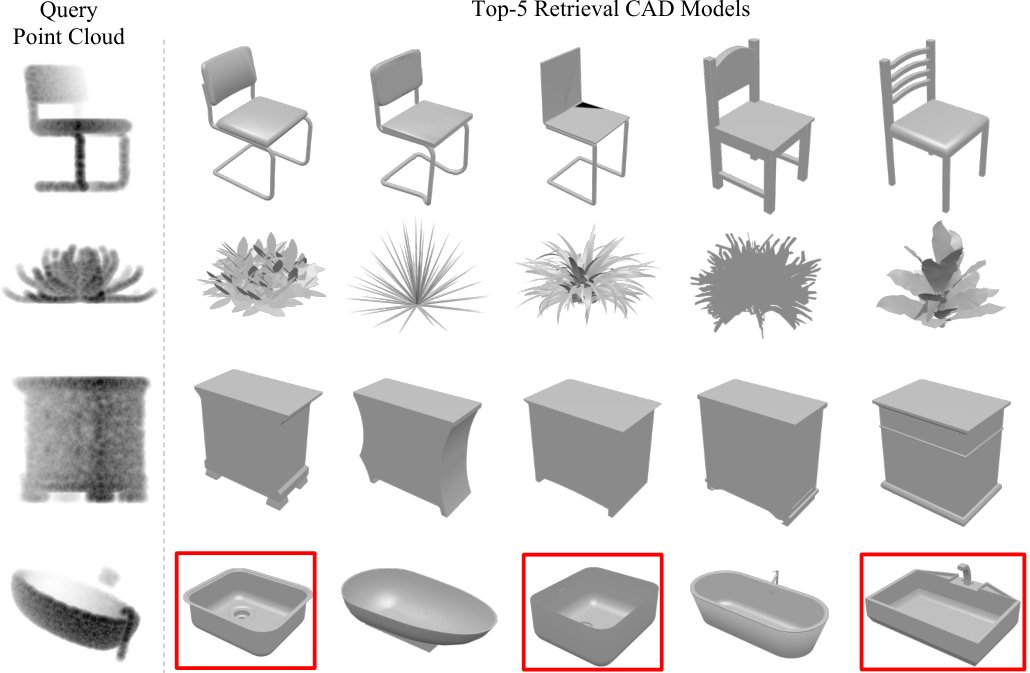
Figure 12: Model retrieval from point cloud. For every given point cloud, we retrieve the top-5 similar shapes from the ModelNet test split. From top to bottom rows, we show examples of chair, plant, nightstand and bathtub queries. Retrieved results that are in wrong category are marked by red boxes.

图12:** 从点云检索模型。 对于每个给定的点云,我们从ModelNet的测试分裂中检索到顶端5的类似形状. 从上到下,我们展示了椅子、植物、睡台和浴缸查询的例子。 错误分类的检索结果用红框标出。 **

Shape Correspondence

In this section, we show that point features learnt by PointNet can be potentially used to compute shape correspondences. Given two shapes, we compute the correspondence between their critical point sets $C_{S}$’s by matching the pairs of points that activate the same dimensions in the global features. Fig 13 and Fig 14 show the detected shape correspondence between two similar chairs and tables.

形状通信

在本节中,我们显示PointNet所学的点特征可以被潜在地用来计算成形的通信. 鉴于两个形状,我们计算它们之间的对应 关键点集 XMATH0XX通过匹配激活全球特征中相同维度的 你是在说: 图13和图14显示了两个相似的椅子和表格之间检测到的形状对应.

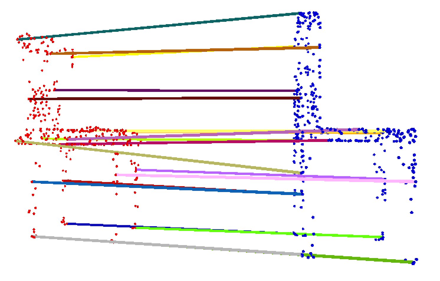
Figure 13: Shape correspondence between two chairs. For the clarity of the visualization, we only show 20 randomly picked correspondence pairs.

图13:** 两位主席之间的联络。 为了清晰的可视化,我们只显示20对随机抽取的函证配对。 **

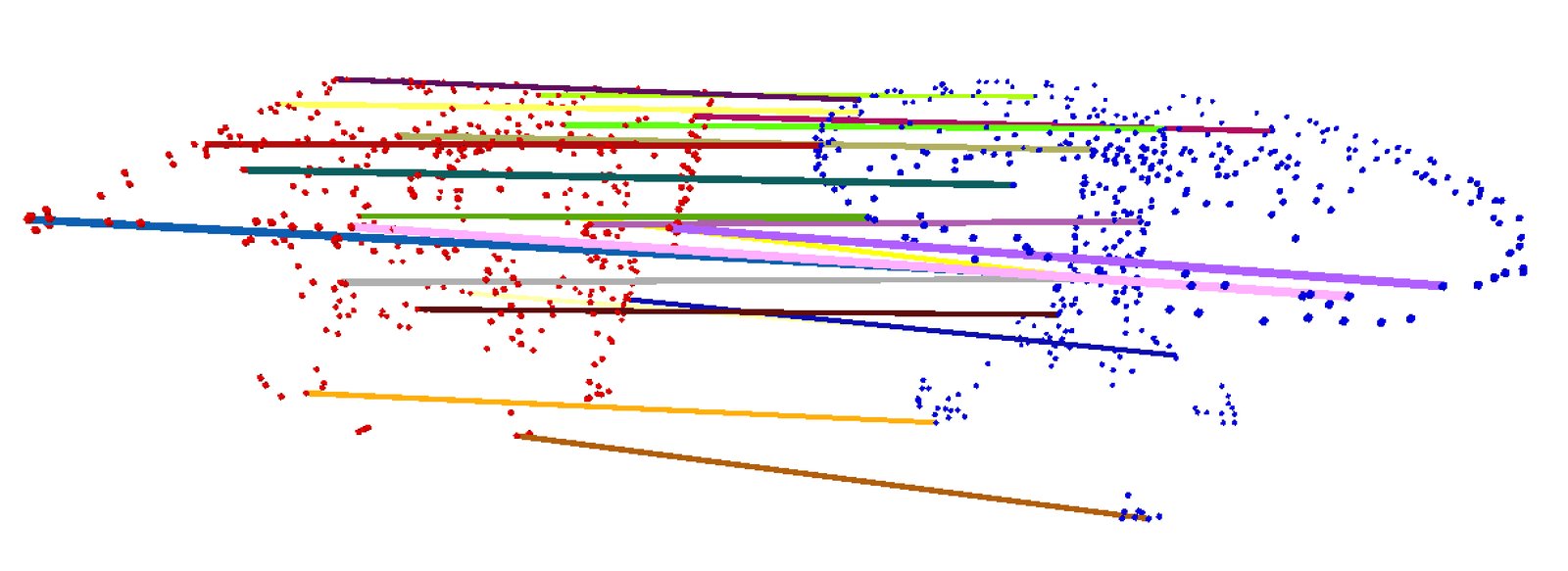
Figure 14: Shape correspondence between two tables. For the clarity of the visualization, we only show 20 randomly picked correspondence pairs.

图14:** 两个表格之间的形状对应。 为了清晰的可视化,我们只显示20对随机抽取的函证配对。 **

Appendix F More Architecture Analysis (Sec 5.2)

附录 F 更多架构分析（第 5.2 节）

Effects of Bottleneck Dimension and Number of Input Points

Here we show our model’s performance change with regard to the size of the first max layer output as well as the number of input points. In Fig 15 we see that performance grows as we increase the number of points however it saturates at around 1K points. The max layer size plays an important role, increasing the layer size from 64 to 1024 results in a $2-4\%$ performance gain. It indicates that we need enough point feature functions to cover the 3D space in order to discriminate different shapes.

QQ Bottleneck 尺寸和输入点数的影响

在这里,我们显示我们的模型在第一最大层输出的大小和输入点数方面的性能变化。 在图15中,我们看到,当我们增加点数时,性能会增加,但是它饱和在1K点左右。 最大层的尺寸馥起重要作用,将层的尺寸从64个增加到1024个,结果产生了$2-4\%$性能增益. 它表明我们需要足够的点特征功能来覆盖3D空间以区别不同的形状.

It’s worth notice that even with 64 points as input (obtained from furthest point sampling on meshes), our network can achieve decent performance.

值得注意的是,即使有64分作为投入(从最远的网点取样中可以发现),我们的网络也能取得体面的性能。

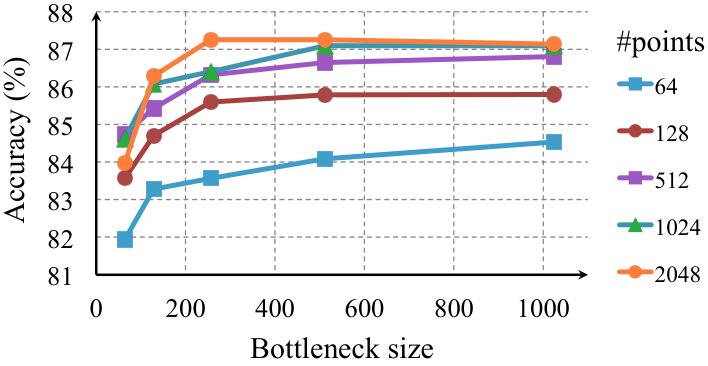
Figure 15: Effects of bottleneck size and number of input points. The metric is overall classification accuracy on ModelNet40 test set.

图15:**瓶颈大小和输入点数的影响。 衡量标准是ModelNet40测试集的总体分类精度。 **

MNIST Digit Classification

While we focus on 3D point cloud learning, a sanity check experiment is to apply our network on a 2D point clouds - pixel sets.

MNIST 数字分类

在我们专注于3D点云学习的同时,一个理智检查实验是将我们的网络应用在2D点云上——像素集上.

To convert an MNIST image into a 2D point set we threshold pixel values and add the pixel (represented as a point with $(x,y)$ coordinate in the image) with values larger than 128 to the set. We use a set size of 256. If there are more than 256 pixels int he set, we randomly sub-sample it; if there are less, we pad the set with the one of the pixels in the set (due to our max operation, which point to use for the padding will not affect outcome).

要将 MNIST 图像转换成2D 点设置,我们将阈值像素值加成像素(在图像中以$(x,y)$坐标的点表示),值大于 128 。 我们使用256的设定尺寸。 如果有超过256像素的英寸,我们随机对它进行子样本;如果有更少的,我们用集中的像素之一来固定设定(因为我们的最大操作,用于粘贴的点不会影响结果).

As seen in Table 7, we compare with a few baselines including multi-layer perceptron that considers input image as an ordered vector, a RNN that consider input as sequence from pixel (0,0) to pixel (27,27), and a vanilla version CNN. While the best performing model on MNIST is still well engineered CNNs (achieving less than $0.3\%$ error rate), it’s interesting to see that our PointNet model can achieve reasonable performance by considering image as a 2D point set.

如眷顾表7所示,我们比较了几个基线,包括将输入图像视为定序矢量的多层透视,将输入视为从像素(0,0)到像素(27,27)的序列的RNN,以及香草版的CNN. 虽然MNIST上的最佳性能模型仍然是设计良好的CNN(实现低于$0.3\%$错误率),但有趣的是,我们的PointNet模型可以通过将图像视为2D点集来实现合理的性能.

	input	error (%)
Multi-layer perceptron [22]	vector	1.60
LeNet5 [12]	image	0.80
Ours PointNet	point set	0.78

Table 7: MNIST classification results. We compare with vanilla versions of other deep architectures to show that our network based on point sets input is achieving reasonable performance on this traditional task.

	投入	错误(%)
多 Ferrari型[22]	向量	1.60
网5[12]	图像	0.80
我们的点网	点集	0.78

表7:** MNIST分类结果。 我们与其他深层建筑的香草版本进行比较,以显示我们基于点集输入的网络正在这一传统任务上取得合理的性能。 **

Normal Estimation

In segmentation version of PointNet, local point features and global feature are concatenated in order to provide context to local points. However, it’s unclear whether the context is learnt through this concatenation. In this experiment, we validate our design by showing that our segmentation network can be trained to predict point normals, a local geometric property that is determined by a point’s neighborhood.

普通估计

在PointNet的分区版本中,局部点特征和全局特征被调和,以便为局部点提供上下文. 然而,目前还不清楚背景是否通过这种结合而得知。 在这个实验中,我们验证了我们的设计,通过显示我们的分块网络可以被训练来预测点的正常现象,一个由点的邻里决定的局部几何属性.

We train a modified version of our segmentation PointNet in a supervised manner to regress to the ground-truth point normals. We just change the last layer of our segmentation PointNet to predict normal vector for each point. We use absolute value of cosine distance as loss.

我们以监督的方式训练一个修改版的分区点网,以倒退到地面真实点的正常状态。 我们只是改变我们的分块点网的最后一层,以预测每个点的正常矢量. 我们使用余弦距离的绝对值作为损失.

Fig. 16 compares our PointNet normal prediction results (the left columns) to the ground-truth normals computed from the mesh (the right columns). We observe a reasonable normal reconstruction. Our predictions are more smooth and continuous than the ground-truth which includes flipped normal directions in some region.

图16 将我们的PointNet正常预测结果(左栏)与从网格(右栏)计算出来的地面真实正常情况进行比较。 我们看到合理的正常重建。 我们的预测比地面真相更平稳和连续,包括某些地区的正常方向翻转。

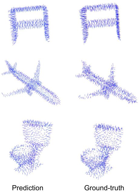
Figure 16: PointNet normal reconstrution results. In this figure, we show the reconstructed normals for all the points in some sample point clouds and the ground-truth normals computed on the mesh.

图16:**PointNet 正常重组结果。 在此图中,我们显示一些样本点云中所有点的重建正常情况以及网点上计算出的地面真实正常情况。 **

Segmentation Robustness

As discussed in Sec 5.2 and Sec B, our PointNet is less sensitive to data corruption and missing points for classification tasks since the global shape feature is extracted from a collection of critical points from the given input point cloud. In this section, we show that the robustness holds for segmentation tasks too. The per-point part labels are predicted based on the combination of per-point features and the learnt global shape feature. In Fig 17, we illustrate the segmentation results for the given input point clouds $S$ (the left-most column), the critical point sets $\mathcal{C}_{S}$ (the middle column) and the upper-bound shapes $\mathcal{N}_{S}$.

• 分块强度

如Sec 5.2和Sec B所述,我们的PointNet对数据腐败和分类任务的缺失点不太敏感,因为全球形状特征是从给定输入点云中收集的关键点 提取出来的。 在这一节中,我们表明,分化任务也坚固有力。 每个点部分的标签是根据每个点的特征与学到的全球形状特征的组合来预测的. 在图17中,我们举例说明给定的输入点云 $S$(最左栏), *临界点集 * $\mathcal{C}_{S}$(中间栏)和 上方的形状的分化结果.$\mathcal{N}_{S}$(英语).

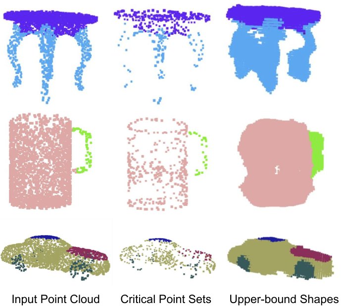
Figure 17: The consistency of segmentation results. We illustrate the segmentation results for some sample given point clouds $S$, their critical point sets $\mathcal{C}_{S}$ and upper-bound shapes $\mathcal{N}_{S}$. We observe that the shape family between the $\mathcal{C}_{S}$ and $\mathcal{N}_{S}$ share a consistent segmentation results.

图17:** 分化结果的一致性。 我们举例说明一些样本的分化结果,即点云$S$、其临界点集 $\mathcal{C}_{S}$和上方形状 $\mathcal{N}_{S}$。 我们注意到,$\mathcal{C}_{S}$和$\mathcal{N}_{S}$之间的形状家族有着一致的分裂结果。 **

Network Generalizability to Unseen Shape Categories

In Fig 18, we visualize the critical point sets and the upper-bound shapes for new shapes from unseen categories (face, house, rabbit, teapot) that are not present in ModelNet or ShapeNet. It shows that the learnt per-point functions are generalizable. However, since we train mostly on man-made objects with lots of planar structures, the reconstructed upper-bound shape in novel categories also contain more planar surfaces.

QQ 网络可通用到不明形状类别

在图18中,我们将“临界点集”和“上限形状”作为新形状的图像,这些形状来自没有出现在ModelNet或ShapeNet中的隐形类别(面部、房屋、兔子、茶壶)。 它表明,每个点所学到的功能是普遍的。 然而,由于我们主要是在人造物体上进行训练,并且有许多浮雕结构,所以在新颖类别中重建的上方形状也包含更多的浮雕表面.

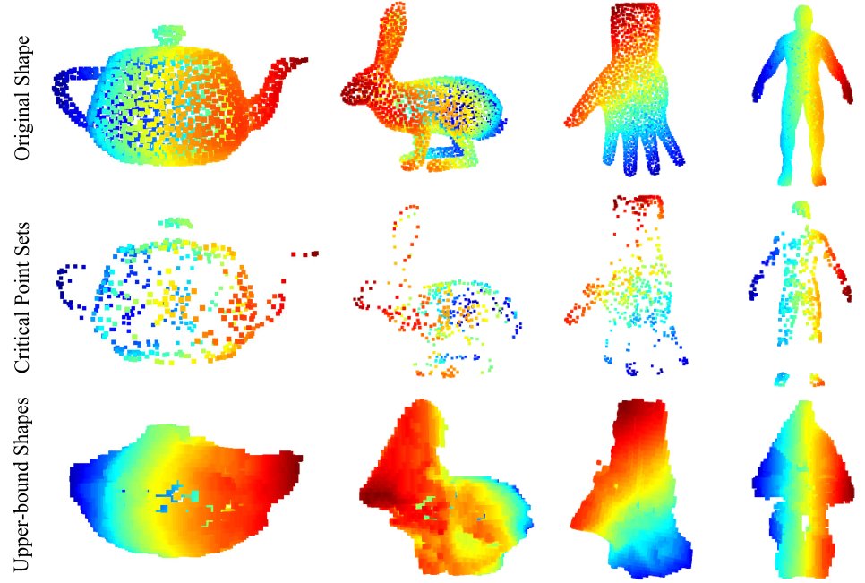
Figure 18: The critical point sets and the upper-bound shapes for unseen objects. We visualize the critical point sets and the upper-bound shapes for teapot, bunny, hand and human body, which are not in the ModelNet or ShapeNet shape repository to test the generalizability of the learnt per-point functions of our PointNet on other unseen objects. The images are color-coded to reflect the depth information.

图18:**不可见物体的临界点集和上方形状。 我们可视化茶壶、兔子、手和人体的“临界点集”和“上限形状”,它们不在ModelNet或ShapeNet形状存储库中,以测试我们PointNet在其他看不见物体上每个点所学到的功能的通用性。 图像的颜色编码是为了反映深度信息。 **

Appendix G Proof of Theorem (Sec 4.3)

附录 G 定理证明（第 4.3 节）

Let $\mathcal{X}=\{S:S\subseteq[0,1]\mbox{ and }|S|=n\}$.

让之一就是$\mathcal{X}=\{S:S\subseteq[0,1]\mbox{ and }|S|=n\}$。

$f:\mathcal{X}\rightarrow\mathbb{R}$ is a continuous function on $\mathcal{X}$ w.r.t to Hausdorff distance $d_{H}(\cdot,\cdot)$ if the following condition is satisfied:

$f:\mathcal{X}\rightarrow\mathbb{R}$在$\mathcal{X}$ w.r.t到Hausdorff距离$d_{H}(\cdot,\cdot)$上是一个连续函数,如果满足以下条件: 1.

$\forall\epsilon>0,\exists\delta>0$, for any $S,S^{\prime}\in\mathcal{X}$, if $d_{H}(S,S^{\prime})<\delta$, then $|f(S)-f(S^{\prime})|<\epsilon$.

$\forall\epsilon>0,\exists\delta>0$,指任何$S,S^{\prime}\in\mathcal{X}$,如果是$d_{H}(S,S^{\prime})<\delta$,然后是$|f(S)-f(S^{\prime})|<\epsilon$.

We show that $f$ can be approximated arbitrarily by composing a symmetric function and a continuous function.

我们显示,$f$可以通过组合对称函数和连续函数来任意地进行近似.

Theorem 1.

Suppose $f:\mathcal{X}\rightarrow\mathbb{R}$ is a continuous set function w.r.t Hausdorff distance $d_{H}(\cdot,\cdot)$. $\forall\epsilon>0$, $\exists$ a continuous function $h$ and a symmetric function $g(x_{1},\dots,x_{n})=\gamma\circ\mbox{MAX}$, where $\gamma$ is a continuous function, MAX is a vector max operator that takes $n$ vectors as input and returns a new vector of the element-wise maximum, such that for any $S\in\mathcal{X}$,

** 定 义 1****。 **

• Suppose $f:\mathcal{X}\rightarrow\mathbb{R}$是一个连续集函数w.r.t Hausdorff距离 $d_{H}(\cdot,\cdot)$. $\forall\epsilon>0$, $\exists$是一个连续函数 $h$和一个对称函数 $g(x_{1},\dots,x_{n})=\gamma\circ\mbox{MAX}$, 其中 $\gamma$是一个连续函数 MAX是一个向量最大运算符,它以$n$向量作为输入并返回元素最大值的新向量,因此对于任何$S\in\mathcal{X}$,*

$$\displaystyle|f(S)-\gamma(\mbox{MAX}(h(x_{1}),\ldots,h(x_{n})))|<\epsilon$$

where $x_{1},\ldots,x_{n}$ are the elements of $S$ extracted in certain order,

$x_{1},\ldots,x_{n}$是按一定顺序提取的$S$的元素,

Proof.

By the continuity of $f$, we take $\delta_{\epsilon}$ so that $|f(S)-f(S^{\prime})|<\epsilon$ for any $S,S^{\prime}\in\mathcal{X}\mbox{ if }d_{H}(S,S^{\prime})<\delta_{\epsilon}$.

将负责证明

除其它外,通过$f$的连续性,我们将$\delta_{\epsilon}$用于任何$S,S^{\prime}\in\mathcal{X}\mbox{ if }d_{H}(S,S^{\prime})<\delta_{\epsilon}$.

Define $K=\lceil 1/\delta_{\epsilon}\rceil$, which split $[0,1]$ into $K$ intervals evenly and define an auxiliary function that maps a point to the left end of the interval it lies in:

定义 $K=\lceil 1/\delta_{\epsilon}\rceil$,将$[0,1]$平分为$K$间隔,并定义一个辅助函数,将它位于间隔的左端的点映射到:

$$\sigma(x)=\frac{\lfloor Kx\rfloor}{K}$$

Let $\tilde{S}=\{\sigma(x):x\in S\}$, then

那就让$\tilde{S}=\{\sigma(x):x\in S\}$吧

$$|f(S)-f(\tilde{S})|<\epsilon$$

because $d_{H}(S,\tilde{S})<1/K\leq\delta_{\epsilon}$.

因为$d_{H}(S,\tilde{S})<1/K\leq\delta_{\epsilon}$。

Let $h_{k}(x)=e^{-d(x,[\frac{k-1}{K},\frac{k}{K}])}$ be a soft indicator function where $d(x,I)$ is the point to set (interval) distance. Let $\mathbf{h}(x)=[h_{1}(x);\ldots;h_{K}(x)]$, then $\mathbf{h}:\mathbb{R}\rightarrow\mathbb{R}^{K}$.

让$h_{k}(x)=e^{-d(x,[\frac{k-1}{K},\frac{k}{K}])}$成为一个软指标函数,其中$d(x,I)$是设置(间)距离的点. 让$\mathbf{h}(x)=[h_{1}(x);\ldots;h_{K}(x)]$,然后是$\mathbf{h}:\mathbb{R}\rightarrow\mathbb{R}^{K}$.

Let $v_{j}(x_{1},\ldots,x_{n})=\max\{\tilde{h}_{j}(x_{1}),\ldots,\tilde{h}_{j}(x_{n})\}$, indicating the occupancy of the $j$-th interval by points in $S$. Let $\mathbf{v}=[v_{1};\ldots;v_{K}]$, then $\mathbf{v}:\underbrace{\mathbb{R}\times\ldots\times\mathbb{R}}_{n}\rightarrow\{0,1\}^{K}$ is a symmetric function, indicating the occupancy of each interval by points in $S$.

让$v_{j}(x_{1},\ldots,x_{n})=\max\{\tilde{h}_{j}(x_{1}),\ldots,\tilde{h}_{j}(x_{n})\}$,在$S$中表示$j$ - 第1次间隔的占用. 让我们$\mathbf{v}=[v_{1};\ldots;v_{K}]$,然后$\mathbf{v}:\underbrace{\mathbb{R}\times\ldots\times\mathbb{R}}_{n}\rightarrow\{0,1\}^{K}$是一个对称函数,在$S$中表示每个间隔的占用点.

Define $\tau:\{0,1\}^{K}\rightarrow\mathcal{X}$ as $\tau(v)=\{\frac{k-1}{K}:v_{k}\geq 1\}$, which maps the occupancy vector to a set which contains the left end of each occupied interval. It is easy to show:

将$\tau:\{0,1\}^{K}\rightarrow\mathcal{X}$定义为$\tau(v)=\{\frac{k-1}{K}:v_{k}\geq 1\}$, 它将占用矢量映射到包含每个正在进行中间隔的左端的集合 。 很容易显示:

$$\displaystyle\tau(\mathbf{v}(x_{1},\ldots,x_{n}))\equiv\tilde{S}$$

where $x_{1},\ldots,x_{n}$ are the elements of $S$ extracted in certain order.

其中$x_{1},\ldots,x_{n}$是按一定顺序提取的$S$的元素.

Let $\gamma:\mathbb{R}^{K}\rightarrow\mathbb{R}$ be a continuous function such that $\gamma(\mathbf{v})=f(\tau(\mathbf{v}))$ for $v\in\{0,1\}^{K}$. Then,

让$\gamma:\mathbb{R}^{K}\rightarrow\mathbb{R}$成为一个连续函数,使$\gamma(\mathbf{v})=f(\tau(\mathbf{v}))$成为$v\in\{0,1\}^{K}$. 礛

$$\displaystyle|\gamma(\mathbf{v}(x_{1},\ldots,x_{n}))-f(S)| \\ \displaystyle= \\ \displaystyle|f(\tau(\mathbf{v}(x_{1},\ldots,x_{n})))-f(S)|<\epsilon$$

Note that $\gamma(\mathbf{v}(x_{1},\ldots,x_{n}))$ can be rewritten as follows:

注意$\gamma(\mathbf{v}(x_{1},\ldots,x_{n}))$可重写如下:

$$\displaystyle\gamma(\mathbf{v}(x_{1},\ldots,x_{n}))= \\ \displaystyle\gamma(\mbox{MAX}(\mathbf{h}(x_{1}),\ldots,\mathbf{h}(x_{n}))) \\ \displaystyle= \\ \displaystyle(\gamma\circ\mbox{MAX})(\mathbf{h}(x_{1}),\ldots,\mathbf{h}(x_{n}))$$

Obviously $\gamma\circ\mbox{MAX}$ is a symmetric function. ∎

显然,$\gamma\circ\mbox{MAX}$是一个对称的函数。

Next we give the proof of Theorem 2. We define $\mathbf{u}=\underset{x_{i}\in S}{\mbox{MAX}}\{h(x_{i})\}$ to be the sub-network of $f$ which maps a point set in $[0,1]^{m}$ to a $K$-dimensional vector. The following theorem tells us that small corruptions or extra noise points in the input set is not likely to change the output of our network:

接下来我们给出定理2的证据. 我们定义$\mathbf{u}=\underset{x_{i}\in S}{\mbox{MAX}}\{h(x_{i})\}$是$f$的子网络,它将$[0,1]^{m}$中的一个点映射到$K$- 维向量. 以下定理告诉我们,输入集中的小腐败或额外噪声点不太可能改变我们网络的输出:

Theorem 2.

Suppose $\mathbf{u}:\mathcal{X}\rightarrow\mathbb{R}^{K}$ such that $\mathbf{u}=\underset{x_{i}\in S}{\mbox{MAX}}\{h(x_{i})\}$ and $f=\gamma\circ\mathbf{u}$. Then,

• 定理2****。 **

• 补充指导指导指导指导指导指导指导指导指导指导指导指导指导指导指导指导指导指导指导指导指导指导指导指导指导指导指导指导指导指导指导指导指导指导指导指导指导指导指导指导指导指导指导指导指导指导指导指导指导指导指导指导指导指导指导指导指导指导指导指导指导指导指导指导指导指导指导指导指导指导指导指导指导指导指导指导指导指导指导指导指导指导指导指导指导指导,指导指导指导指导指导指导指导指导指导指导指导指导指导指导指导指导指导指导指导指导指导指导指导指导指导指导指导指导指导指导指导指导指导指导指导指导指导指导指导指导指导指导指导指导指导指导指导指导指导指导指导指导指导指导指导指导指导指导指导指导指导指导指导指导指导指导指导指导指导指导指导指导指导指导指导指导指导指导指导指导指导指导指导指导指导指导指导指导指导指导指导指导指导指导指导,指导指导指导指导指导指导指导指导指导指导指导指导指导指导指导指导,指导指导指导指导指导指导指导指导指导指导指导指导指导指导指导指导指导指导指导指导指导指导,指导指导指导指导指导指导指导指导指导指导指导指导指导指导指导指导指导指导指导指导指导指导指导指导指导指导指导指导指导指导

(a) $\forall S,\exists~\mathcal{C}_{S},\mathcal{N}_{S}\subseteq\mathcal{X}$,$f(T)=f(S)$if$\mathcal{C}_{S}\subseteq T\subseteq\mathcal{N}_{S}$;
(b) $|\mathcal{C}_{S}|\leq K$

(a)$\forall S,\exists~\mathcal{C}_{S},\mathcal{N}_{S}\subseteq\mathcal{X}$,$f(T)=f(S)$,$\mathcal{C}_{S}\subseteq T\subseteq\mathcal{N}_{S}$*;
(b) XIMATH3XX

Proof.

Obviously, $\forall S\in\mathcal{X}$, $f(S)$ is determined by $\mathbf{u}(S)$. So we only need to prove that $\forall S,\exists\,\mathcal{C}_{S},\mathcal{N}_{S}\subseteq\mathcal{X},f(T)=f(S)\,\mbox{if}\,\mathcal{C}_{S}\subseteq T\subseteq\mathcal{N}_{S}$.

证明

显然,$\forall S\in\mathcal{X}$,$f(S)$是由$\mathbf{u}(S)$决定的. 所以我们只需要证明$\forall S,\exists\,\mathcal{C}_{S},\mathcal{N}_{S}\subseteq\mathcal{X},f(T)=f(S)\,\mbox{if}\,\mathcal{C}_{S}\subseteq T\subseteq\mathcal{N}_{S}$。

For the $j$th dimension as the output of $\mathbf{u}$, there exists at least one $x_{j}\in\mathcal{X}$ such that $h_{j}(x_{j})=\mathbf{u}_{j}$, where $h_{j}$ is the $j$th dimension of the output vector from $h$. Take $\mathcal{C}_{S}$ as the union of all $x_{j}$ for $j=1,\ldots,K$. Then, $\mathcal{C}_{S}$ satisfies the above condition.

对于$j$th维度作为$\mathbf{u}$的输出,至少存在一个$x_{j}\in\mathcal{X}$,即$h_{j}(x_{j})=\mathbf{u}_{j}$,其中$h_{j}$是$h$输出矢量的$j$th维度. 以$\mathcal{C}_{S}$为$x_{j}$全体的联盟. 然后,$\mathcal{C}_{S}$满足上述条件.

Adding any additional points $x$ such that $h(x)\leq\mathbf{u}(S)$ at all dimensions to $\mathcal{C}_{S}$ does not change $\mathbf{u}$, hence $f$. Therefore, $\mathcal{T}_{S}$ can be obtained adding the union of all such points to $\mathcal{N}_{S}$.

在XXMATH0 XX中添加任何额外的点,使$h(x)\leq\mathbf{u}(S)$在所有维度上都不变$\mathbf{u}$,因此$f$. 因此,可以取得$\mathcal{T}_{S}$,将所有这些点加到$\mathcal{N}_{S}$。

∎

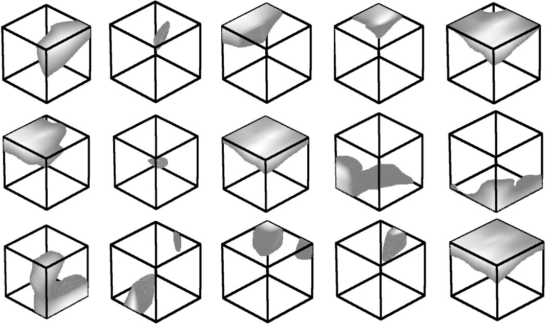
Figure 19: Point function visualization. For each per-point function $h$, we calculate the values $h(p)$ for all the points $p$ in a cube of diameter two located at the origin, which spatially covers the unit sphere to which our input shapes are normalized when training our PointNet. In this figure, we visualize all the points $p$ that give $h(p)>0.5$ with function values color-coded by the brightness of the voxel. We randomly pick 15 point functions and visualize the activation regions for them.

图19:**点函数可视化。 对于每个点函数$h$,我们对位于源头的直径2的立方体中所有点值$h(p)$进行计算,在空间上涵盖了我们在训练我们的PointNet时,输入形状正常化的单位球体. 在这个图中,我们可视化所有给$p$的点,以阴道的亮度编码的函数值为$h(p)>0.5$. 我们随机选取15个点的功能,为它们可视化激活区域。

Appendix H More Visualizations

附录 H 更多可视化

Classification Visualization

We use t-SNE[15] to embed point cloud global signature (1024-dim) from our classification PointNet into a 2D space. Fig 20 shows the embedding space of ModelNet 40 test split shapes. Similar shapes are clustered together according to their semantic categories.

• 分类可视化

我们使用 t-SNE[15]联合国宪章将点云全球签名(1024- 87.dim)从我们的分类点网嵌入一个2D空间. 图20显示了ModelNet 40测试分裂形状的嵌入空间. 类似的形状按照它们的语义分类组合在一起.

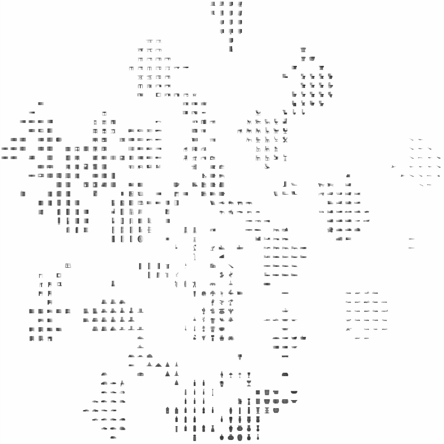
Figure 20: 2D embedding of learnt shape global features. We use t-SNE technique to visualize the learnt global shape features for the shapes in ModelNet40 test split.

图20:**2D 嵌入已学到的形状全球特征。发展中国家和转型期经济国家联盟

Segmentation Visualization

We present more segmentation results on both complete CAD models and simulated Kinect partial scans. We also visualize failure cases with error analysis. Fig 21 and Fig 22 show more segmentation results generated on complete CAD models and their simulated Kinect scans. Fig 23 illustrates some failure cases. Please read the caption for the error analysis.

• 分块可视化

我们在完整的CAD模型和模拟的Kinect部分扫描上呈现了更多的分解结果. 我们还通过错误分析来想象故障情况。 图21和图22显示在完整的CAD模型及其模拟Kinect扫描上产生的分解结果更多. 图23说明了一些失败案例。 请阅读错误分析的标题 。

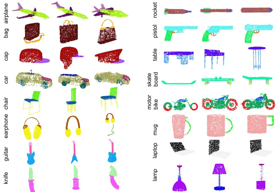
Figure 21: PointNet segmentation results on complete CAD models.

图21:**完整CAD模型的PointNet分割结果。 **

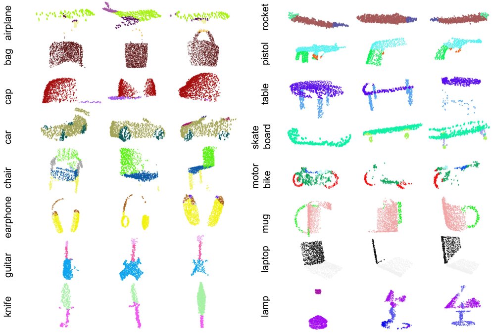
Figure 22: PointNet segmentation results on simulated Kinect scans.

图22:町网模拟Kinect扫描结果**

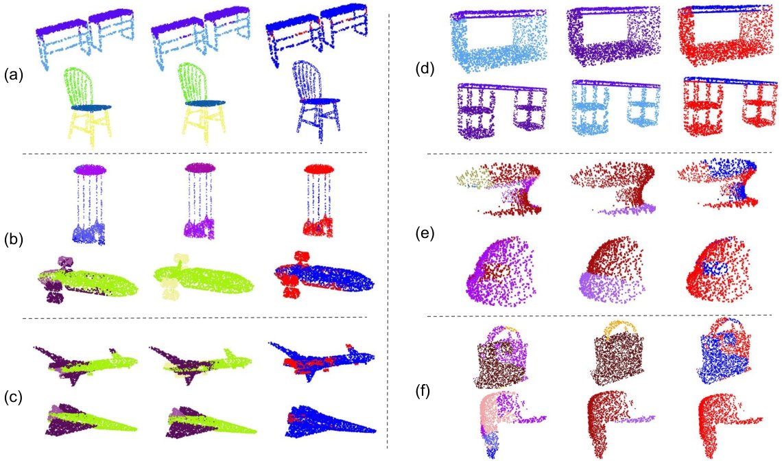
Figure 23: PointNet segmentation failure cases. In this figure, we summarize six types of common errors in our segmentation application. The prediction and the ground-truth segmentations are given in the first and second columns, while the difference maps are computed and shown in the third columns. The red dots correspond to the wrongly labeled points in the given point clouds. (a) illustrates the most common failure cases: the points on the boundary are wrongly labeled. In the examples, the label predictions for the points near the intersections between the table/chair legs and the tops are not accurate. However, most segmentation algorithms suffer from this error. (b) shows the errors on exotic shapes. For examples, the chandelier and the airplane shown in the figure are very rare in the data set. (c) shows that small parts can be overwritten by nearby large parts. For example, the jet engines for airplanes (yellow in the figure) are mistakenly classified as body (green) or the plane wing (purple). (d) shows the error caused by the inherent ambiguity of shape parts. For example, the two bottoms of the two tables in the figure are classified as table legs and table bases (category other in [29]), while ground-truth segmentation is the opposite. (e) illustrates the error introduced by the incompleteness of the partial scans. For the two caps in the figure, almost half of the point clouds are missing. (f) shows the failure cases when some object categories have too less training data to cover enough variety. There are only 54 bags and 39 caps in the whole dataset for the two categories shown here.

图23:*PointNet拆分失败案例。 在这个图中,我们总结了我们分解应用中的六种常见错误. 第一栏和第二栏给出了预测和地面真实分解,而差异图则在第三栏计算和显示。 红色点对应给定点云中的错标点. (a)说明最常见的故障情况:边界上的点错标. 在例子中,表/椅腿与顶部交汇点附近的标签预测不准确. 然而,大多数分化算法都存在这种错误。 (b) 显示异域形状的错误。 例如,图中显示的吊灯和飞机在数据集中非常罕见。 (c) 显示小部分可能被附近的大部分覆盖。 例如,飞机的喷气发动机(图中的黄色)被错误地hybody(绿色)或平面翼(purple)分类. (d)显示了形状部件固有的模糊性所造成的错误. 例如,图中两个表格的两个底部被归类为表腿和表基([29]中的其他*类),而地面-真相分割则相反. (e) 说明部分扫描不完整造成的错误。 对于图中的两顶盖,几乎一半的点 我们还缺点云. (f) 显示失败情况,因为某些对象类别的培训数据太少,无法涵盖足够的多样性。 整个数据集中只有54个袋和39个盖,用于此处所示的两类。 **

Scene Semantic Parsing Visualization

We give a visualization of semantic parsing in Fig 24 where we show input point cloud, prediction and ground truth for both semantic segmentation and object detection for two office rooms and one conference room. The area and the rooms are unseen in the training set.

*臀部语义解析可视化

在图24中,我们对语义解析进行可视化分析,在图24中,我们显示输入点云、预测和地面真相,用于两个办公室和一个会议室的语义解析和物体探测。 训练场里看不到现场和房间。

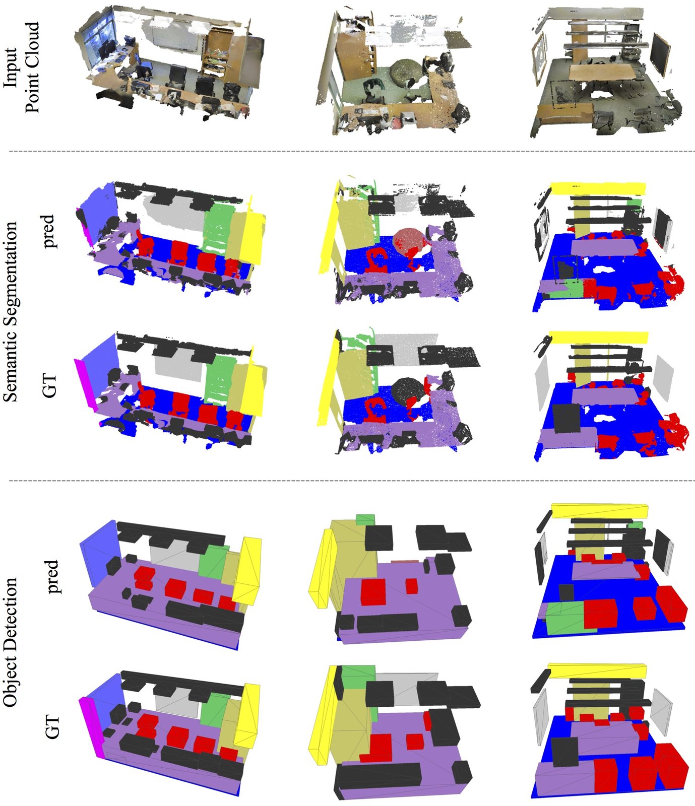
Figure 24: Examples of semantic segmentation and object detection. First row is input point cloud, where walls and ceiling are hided for clarity. Second and third rows are prediction and ground-truth of semantic segmentation on points, where points belonging to different semantic regions are colored differently (chairs in red, tables in purple, sofa in orange, board in gray, bookcase in green, floors in blue, windows in violet, beam in yellow, column in magenta, doors in khaki and clutters in black). The last two rows are object detection with bounding boxes, where predicted boxes are from connected components based on semantic segmentation prediction.

图24:语义分解和物体检测实例. 第一行是输入点云,其中墙壁和天花板被隐藏,以明晰. 第二行和第三行是对各点的语义分解的预测和地面真实性,属于不同语义区域的分点颜色不同(主席为红色,桌子为紫色,沙发为橙色,书架为灰色,书架为绿色,地板为蓝色,窗户为紫色,梁为黄色,柱为紫红色,门为卡其色,十字花为黑色)。 最后两行是带有边框的物体检测,其中预测的箱来自基于语义分区预测的连接组件.

Point Function Visualization

Our classification PointNet computes $K$ (we take $K=1024$ in this visualization) dimension point features for each point and aggregates all the per-point local features via a max pooling layer into a single $K$-dim vector, which forms the global shape descriptor.

XQ点函数可视dong

我们的分类点网计算了每个点的$K$(在这个可视化中我们取$K=1024$)维度点特征,并通过最大集合层将每个点的所有局部特征汇总到一个单一的$K$ - dim矢量中,形成全局形状描述符.

To gain more insights on what the learnt per-point functions $h$’s detect, we visualize the points $p_{i}$’s that give high per-point function value $f(p_{i})$ in Fig 19. This visualization clearly shows that different point functions learn to detect for points in different regions with various shapes scattered in the whole space.

为了更深入地了解$h$的每点函数的检测结果,我们将图19中的$p_{i}$的每点函数值高的点进行直观化. 这种可视化明确显示,不同的点函数会学习检测不同区域中分散在整个空间中的各种形状的点.