Pointer Networks

指针网络

Oriol Vinyals Thanks:  Equal contribution Affiliation:  Google Brain    Meire Fortunato † † footnotemark: Affiliation:  Department of Mathematics, UC Berkeley    Navdeep Jaitly Affiliation:  Google Brain

Abstract

摘要

We introduce a new neural architecture to learn the conditional probability of an output sequence with elements that are discrete tokens corresponding to positions in an input sequence. Such problems cannot be trivially addressed by existent approaches such as sequence-to-sequence [1] and Neural Turing Machines [2], because the number of target classes in each step of the output depends on the length of the input, which is variable. Problems such as sorting variable sized sequences, and various combinatorial optimization problems belong to this class. Our model solves the problem of variable size output dictionaries using a recently proposed mechanism of neural attention. It differs from the previous attention attempts in that, instead of using attention to blend hidden units of an encoder to a context vector at each decoder step, it uses attention as a pointer to select a member of the input sequence as the output. We call this architecture a Pointer Net (Ptr-Net). We show Ptr-Nets can be used to learn approximate solutions to three challenging geometric problems – finding planar convex hulls, computing Delaunay triangulations, and the planar Travelling Salesman Problem – using training examples alone. Ptr-Nets not only improve over sequence-to-sequence with input attention, but also allow us to generalize to variable size output dictionaries. We show that the learnt models generalize beyond the maximum lengths they were trained on. We hope our results on these tasks will encourage a broader exploration of neural learning for discrete problems.

我们提出一种新的神经网络结构，用来学习输出序列的条件概率；该输出序列的元素是离散记号，分别对应于输入序列中的位置。这类问题无法被现有方法轻易处理，例如序列到序列 [1] 与神经图灵机（Neural Turing Machines）[2]，因为输出每一步的目标类别数取决于输入的长度，而这个长度是可变的。对可变长度序列排序，以及多种组合优化问题，都属于这一类。我们的模型借助最近提出的神经注意力机制，解决了输出词典大小可变的问题。它与以往注意力用法的不同之处在于：不是在解码器每一步用注意力把编码器隐单元混合成上下文向量，而是把注意力当作指针，从输入序列中选出一个成员作为输出。我们把这种结构称为 Pointer Net（Ptr-Net）。我们表明，仅用训练样本，Ptr-Net 就能学到三个有挑战性的几何问题的近似解：求平面凸包、计算 Delaunay 三角剖分，以及平面旅行商问题（TSP）。Ptr-Net 不仅优于带输入注意力的序列到序列模型，还能推广到可变大小的输出词典。我们还表明，学到的模型可以推广到超过其训练时最大长度的实例。希望这些任务上的结果，能推动人们更广泛地探索用神经方法学习离散问题。

1 Introduction

1 引言

Recurrent Neural Networks (RNNs) have been used for learning functions over sequences from examples for more than three decades [3]. However, their architecture limited them to settings where the inputs and outputs were available at a fixed frame rate (e.g. [4]). The recently introduced sequence-to-sequence paradigm [1] removed these constraints by using one RNN to map an input sequence to an embedding and another (possibly the same) RNN to map the embedding to an output sequence. Bahdanau et. al. augmented the decoder by propagating extra contextual information from the input using a content-based attentional mechanism [5, 2, 6]. These developments have made it possible to apply RNNs to new domains, achieving state-of-the-art results in core problems in natural language processing such as translation [1, 5] and parsing [7], image and video captioning [8, 9], and even learning to execute small programs [2, 10].

循环神经网络（RNN）从样本中学习序列上的函数，已经用了三十多年 [3]。不过，它们的结构把应用限制在输入和输出都以固定帧率给出的设定（例如 [4]）。最近提出的序列到序列范式 [1] 打破了这些限制：用一个 RNN 把输入序列映射到嵌入，再用另一个（也可以是同一个）RNN 把该嵌入映射成输出序列。Bahdanau 等人通过基于内容的注意力机制，把来自输入的额外上下文信息传给解码器 [5, 2, 6]。这些进展使 RNN 能进入新的领域，并在自然语言处理的核心问题上取得当时最好的结果，例如翻译 [1, 5] 和句法分析 [7]，图像与视频描述 [8, 9]，甚至学习执行小型程序 [2, 10]。

Nonetheless, these methods still require the size of the output dictionary to be fixed a priori. Because of this constraint we cannot directly apply this framework to combinatorial problems where the size of the output dictionary depends on the length of the input sequence. In this paper, we address this limitation by repurposing the attention mechanism of [5] to create pointers to input elements. We show that the resulting architecture, which we name Pointer Networks (Ptr-Nets), can be trained to output satisfactory solutions to three combinatorial optimization problems – computing planar convex hulls, Delaunay triangulations and the symmetric planar Travelling Salesman Problem (TSP). The resulting models produce approximate solutions to these problems in a purely data driven fashion (i.e., when we only have examples of inputs and desired outputs). The proposed approach is depicted in Figure 1.

尽管如此，这些方法仍然要求输出词典的大小事先固定。由于这一约束，我们无法把该框架直接用到组合问题上——在那些问题里，输出词典的大小取决于输入序列的长度。本文通过重新利用 [5] 的注意力机制来生成指向输入元素的指针，以克服这一限制。我们表明，由此得到的结构——我们称之为指针网络（Pointer Networks，Ptr-Nets）——可以训练出来，为三个组合优化问题输出令人满意的解：计算平面凸包、Delaunay 三角剖分，以及对称的平面旅行商问题（TSP）。得到的模型以纯数据驱动的方式（也就是说，我们只有输入和期望输出的样本）为这些问题产生近似解。所提出的方法如图 1 所示。

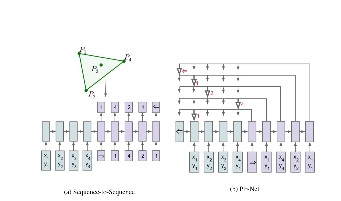
Figure 1: (a) Sequence-to-Sequence - An RNN (blue) processes the input sequence to create a code vector that is used to generate the output sequence (purple) using the probability chain rule and another RNN. The output dimensionality is fixed by the dimensionality of the problem and it is the same during training and inference [1]. (b) Ptr-Net - An encoding RNN converts the input sequence to a code (blue) that is fed to the generating network (purple). At each step, the generating network produces a vector that modulates a content-based attention mechanism over inputs ([5, 2]). The output of the attention mechanism is a softmax distribution with dictionary size equal to the length of the input.

图 1：(a) 序列到序列——一个 RNN（蓝色）处理输入序列，得到一个编码向量，再按概率链式法则用另一个 RNN 生成输出序列（紫色）。输出维数由问题本身的维数固定，训练和推断时相同 [1]。(b) Ptr-Net——一个编码 RNN 把输入序列转换成编码（蓝色），再送入生成网络（紫色）。每一步，生成网络产生一个向量，用来调制作用在输入上的基于内容的注意力机制（[5, 2]）。注意力机制的输出是一个 softmax 分布，其词典大小等于输入长度。

The main contributions of our work are as follows:

我们工作的主要贡献如下：

• • We propose a new architecture, that we call Pointer Net, which is simple and effective. It deals with the fundamental problem of representing variable length dictionaries by using a softmax probability distribution as a “pointer”.

• • 我们提出一种新结构，称之为 Pointer Net，它既简单又有效。它用 softmax 概率分布当作“指针”，来处理表示可变长度词典这一基本问题。

• • We apply the Pointer Net model to three distinct non-trivial algorithmic problems involving geometry. We show that the learned model generalizes to test problems with more points than the training problems.

• • 我们把 Pointer Net 用到三个互不相同、且并不平凡的几何算法问题上。我们表明，学到的模型可以推广到点数比训练问题更多的测试问题。

• • Our Pointer Net model learns a competitive small scale ($n\leq 50$) TSP approximate solver. Our results demonstrate that a purely data driven approach can learn approximate solutions to problems that are computationally intractable.

• • 我们的 Pointer Net 学到了一个有竞争力的小规模（$n\leq 50$）TSP 近似求解器。结果表明，纯数据驱动的方法也能为计算上难解的问题学到近似解。

2 Models

2 模型

We review the sequence-to-sequence [1] and input-attention models [5] that are the baselines for this work in Sections  2.1 and 2.2. We then describe our model - Ptr-Net in Section 2.3.

我们在第 2.1 节和第 2.2 节回顾作为本研究基线的序列到序列 [1] 与输入注意力模型 [5]。随后在第 2.3 节描述我们的模型 Ptr-Net。

2.1 Sequence-to-Sequence Model

2.1 序列到序列模型

Given a training pair, $(\mathcal{P},\mathcal{C}^{\mathcal{P}})$, the sequence-to-sequence model computes the conditional probability $p(\mathcal{C}^{\mathcal{P}}|\mathcal{P};\theta)$ using a parametric model (an RNN with parameters $\theta$) to estimate the terms of the probability chain rule (also see Figure 1), i.e.

给定一对训练样本 $(\mathcal{P},\mathcal{C}^{\mathcal{P}})$，序列到序列模型用一个参数化模型（带参数 $\theta$ 的 RNN）来估计概率链式法则中的各项，从而计算条件概率 $p(\mathcal{C}^{\mathcal{P}}|\mathcal{P};\theta)$（也可参见图 1），即

$$p(\mathcal{C}^{\mathcal{P}}|\mathcal{P};\theta)=\prod_{i=1}^{m(\mathcal{P})}p_{\theta}(C_{i}|C_{1},\ldots,C_{i-1},\mathcal{P};\theta). \tag{1}$$

Here $\mathcal{P}=\{P_{1},\dots,P_{n}\}$ is a sequence of $n$ vectors and $\mathcal{C}^{\mathcal{P}}=\{C_{1},\dots,C_{m(\mathcal{P})}\}$ is a sequence of $m(\mathcal{P})$ indices, each between 1 and $n$.

这里 $\mathcal{P}=\{P_{1},\dots,P_{n}\}$ 是由 $n$ 个向量组成的序列，$\mathcal{C}^{\mathcal{P}}=\{C_{1},\dots,C_{m(\mathcal{P})}\}$ 是由 $m(\mathcal{P})$ 个下标组成的序列，每个下标都介于 1 与 $n$ 之间。

The parameters of the model are learnt by maximizing the conditional probabilities for the training set, i.e.

模型参数通过对训练集的条件概率求极大来学习，即

$$\theta^{*}=\argmax_{\theta}\sum_{\mathcal{P},\mathcal{C}^{\mathcal{P}}}\log p(\mathcal{C}^{\mathcal{P}}|\mathcal{P};\theta), \tag{2}$$

where the sum is over training examples.

其中求和遍历各个训练样本。

As in [1], we use an Long Short Term Memory (LSTM) [11] to model $p_{\theta}(C_{i}|C_{1},\ldots,C_{i-1},\mathcal{P};\theta)$. The RNN is fed $P_{i}$ at each time step, $i$, until the end of the input sequence is reached, at which time a special symbol, $\Rightarrow$ is input to the model. The model then switches to the generation mode until the network encounters the special symbol $\Leftarrow$, which represents termination of the output sequence.

与 [1] 一样，我们用长短期记忆网络（LSTM）[11] 来建模 $p_{\theta}(C_{i}|C_{1},\ldots,C_{i-1},\mathcal{P};\theta)$。RNN 在每个时间步 $i$ 读入 $P_{i}$，直到输入序列结束；此时向模型输入一个特殊记号 $\Rightarrow$。随后模型转入生成模式，直到网络遇到表示输出序列终止的特殊记号 $\Leftarrow$。

Note that this model makes no statistical independence assumptions. We use two separate RNNs (one to encode the sequence of vectors $P_{j}$, and another one to produce or decode the output symbols $C_{i}$). We call the former RNN the encoder and the latter the decoder or the generative RNN.

注意，这一模型并不做统计独立性假设。我们使用两个分开的 RNN（一个编码向量序列 $P_{j}$，另一个产生或解码输出记号 $C_{i}$）。我们把前者称为编码器，把后者称为解码器或生成 RNN。

During inference, given a sequence ${\mathcal{P}}$, the learnt parameters $\theta^{*}$ are used to select the sequence $\mathcal{\hat{C}}^{\mathcal{P}}$ with the highest probability, i.e., $\displaystyle{\mathcal{\hat{C}}}^{\mathcal{P}}=\argmax_{\mathcal{C}^{\mathcal{P}}}p(\mathcal{C}^{\mathcal{P}}|\mathcal{P};\theta^{*}).$ Finding the optimal sequence $\mathcal{\hat{C}}$ is computationally impractical because of the combinatorial number of possible output sequences. Instead we use a beam search procedure to find the best possible sequence given a beam size.

推断时，给定序列 ${\mathcal{P}}$，用学到的参数 $\theta^{*}$ 选出条件概率最高的序列 $\mathcal{\hat{C}}^{\mathcal{P}}$，即 $\displaystyle{\mathcal{\hat{C}}}^{\mathcal{P}}=\argmax_{\mathcal{C}^{\mathcal{P}}}p(\mathcal{C}^{\mathcal{P}}|\mathcal{P};\theta^{*})$。由于可能的输出序列数量是组合级的，寻找最优序列 $\mathcal{\hat{C}}$ 在计算上不可行。我们改用束搜索（beam search），在给定束宽下寻找尽可能好的序列。

In this sequence-to-sequence model, the output dictionary size for all symbols $C_{i}$ is fixed and equal to $n$, since the outputs are chosen from the input. Thus, we need to train a separate model for each $n$. This prevents us from learning solutions to problems that have an output dictionary with a size that depends on the input sequence length.

在这一序列到序列模型中，所有记号 $C_{i}$ 的输出词典大小是固定的，并且等于 $n$，因为输出都是从输入中选出的。因此，我们对每个 $n$ 都需要单独训练一个模型。这使我们无法学习那些输出词典大小取决于输入序列长度的问题。

Under the assumption that the number of outputs is $O(n)$ this model has computational complexity of $O(n)$. However, exact algorithms for the problems we are dealing with are more costly. For example, the convex hull problem has complexity $O(n\log n)$. The attention mechanism (see Section 2.2) adds more “computational capacity” to this model.

在输出个数为 $O(n)$ 的假定下，该模型的计算复杂度是 $O(n)$。不过，我们面对的这些问题的精确算法代价更高。例如，凸包问题的复杂度是 $O(n\log n)$。注意力机制（见第 2.2 节）为这一模型增加了更多“计算容量”。

2.2 Content Based Input Attention

2.2 基于内容的输入注意力

The vanilla sequence-to-sequence model produces the entire output sequence $\mathcal{C}^{\mathcal{P}}$ using the fixed dimensional state of the recognition RNN at the end of the input sequence $\mathcal{P}$. This constrains the amount of information and computation that can flow through to the generative model. The attention model of [5] ameliorates this problem by augmenting the encoder and decoder RNNs with an additional neural network that uses an attention mechanism over the entire sequence of encoder RNN states.

朴素的序列到序列模型只用识别 RNN 在输入序列 $\mathcal{P}$ 结束时的固定维状态，来产生整个输出序列 $\mathcal{C}^{\mathcal{P}}$。这限制了能够流向生成模型的信息量和计算量。[5] 的注意力模型通过给编码器和解码器 RNN 增加另一个神经网络来缓解这一问题，该网络对编码器 RNN 的整段状态序列使用注意力机制。

For notation purposes, let us define the encoder and decoder hidden states as $(e_{1},\ldots,e_{n})$ and $(d_{1},\ldots,d_{m(\mathcal{P})})$, respectively. For the LSTM RNNs, we use the state after the output gate has been component-wise multiplied by the cell activations. We compute the attention vector at each output time $i$ as follows:

为便于表述，我们把编码器和解码器的隐状态分别记为 $(e_{1},\ldots,e_{n})$ 和 $(d_{1},\ldots,d_{m(\mathcal{P})})$。对于 LSTM 这类 RNN，我们使用输出门与细胞激活逐分量相乘之后的状态。我们在每个输出时刻 $i$ 按如下方式计算注意力向量：

$$\displaystyle u^{i}_{j} \\ \displaystyle= \\ \displaystyle v^{T}\tanh(W_{1}e_{j}+W_{2}d_{i})\quad j\in(1,\ldots,n) \\ \displaystyle a^{i}_{j} \\ \displaystyle= \\ \displaystyle\text{softmax}(u^{i}_{j})\quad\qquad\qquad\quad j\in(1,\ldots,n) \\ \displaystyle d^{\prime}_{i} \\ \displaystyle= \\ \displaystyle\sum_{j=1}^{n}a^{i}_{j}e_{j} \tag{3}$$

where softmax normalizes the vector $u^{i}$ (of length $n$) to be the “attention” mask over the inputs, and $v$, $W_{1}$, and $W_{2}$ are learnable parameters of the model. In all our experiments, we use the same hidden dimensionality at the encoder and decoder (typically 512), so $v$ is a vector and $W_{1}$ and $W_{2}$ are square matrices. Lastly, $d^{\prime}_{i}$ and $d_{i}$ are concatenated and used as the hidden states from which we make predictions and which we feed to the next time step in the recurrent model.

其中 softmax 把长度为 $n$ 的向量 $u^{i}$ 归一化，使之成为覆盖各个输入的“注意力”掩码；$v$、$W_{1}$ 和 $W_{2}$ 是模型中可学习的参数。在我们所有实验中，编码器与解码器使用相同的隐状态维数（通常是 512），因此 $v$ 是向量，$W_{1}$ 和 $W_{2}$ 是方阵。最后，把 $d^{\prime}_{i}$ 与 $d_{i}$ 拼接起来，既作为我们做预测所用的隐状态，也作为送入循环模型下一时间步的隐状态。

Note that for each output we have to perform $n$ operations, so the computational complexity at inference time becomes $O(n^{2})$.

注意，每产生一个输出都要做 $n$ 次运算，因此推断时的计算复杂度变成 $O(n^{2})$。

This model performs significantly better than the sequence-to-sequence model on the convex hull problem, but it is not applicable to problems where the output dictionary size depends on the input.

在凸包问题上，这一模型明显优于序列到序列模型，但它无法用于输出词典大小取决于输入的问题。

Nevertheless, a very simple extension (or rather reduction) of the model allows us to do this easily.

不过，对该模型做一个非常简单的扩展（或者说简化），我们就能轻松做到这一点。

2.3 Ptr-Net

We now describe a very simple modification of the attention model that allows us to apply the method to solve combinatorial optimization problems where the output dictionary size depends on the number of elements in the input sequence.

我们现在描述对注意力模型的一个非常简单的修改，使该方法能够用于输出词典大小取决于输入序列元素个数的组合优化问题。

The sequence-to-sequence model of Section 2.1 uses a softmax distribution over a fixed sized output dictionary to compute $p(C_{i}|C_{1},\ldots,C_{i-1},\mathcal{P})$ in Equation 1. Thus it cannot be used for our problems where the size of the output dictionary is equal to the length of the input sequence. To solve this problem we model $p(C_{i}|C_{1},\ldots,C_{i-1},\mathcal{P})$ using the attention mechanism of Equation 3 as follows:

第 2.1 节的序列到序列模型用定义在固定大小输出词典上的 softmax 分布，来计算公式 1 中的 $p(C_{i}|C_{1},\ldots,C_{i-1},\mathcal{P})$。因此，它不能用于我们的问题：这里输出词典的大小等于输入序列的长度。为解决这一问题，我们用公式 3 中的注意力机制来建模 $p(C_{i}|C_{1},\ldots,C_{i-1},\mathcal{P})$，具体如下：

$$\displaystyle u^{i}_{j} \\ \displaystyle= \\ \displaystyle v^{T}\tanh(W_{1}e_{j}+W_{2}d_{i})\quad j\in(1,\ldots,n) \\ \displaystyle p(C_{i}|C_{1},\ldots,C_{i-1},\mathcal{P}) \\ \displaystyle= \\ \displaystyle\text{softmax}(u^{i})$$

where softmax normalizes the vector $u^{i}$ (of length $n$) to be an output distribution over the dictionary of inputs, and $v$, $W_{1}$, and $W_{2}$ are learnable parameters of the output model. Here, we do not blend the encoder state $e_{j}$ to propagate extra information to the decoder, but instead, use $u^{i}_{j}$ as pointers to the input elements. In a similar way, to condition on $C_{i-1}$ as in Equation 1, we simply copy the corresponding $P_{C_{i-1}}$ as the input. Both our method and the attention model can be seen as an application of content-based attention mechanisms proposed in [6, 5, 2].

其中 softmax 把长度为 $n$ 的向量 $u^{i}$ 归一化，使之成为定义在输入词典上的输出分布；$v$、$W_{1}$ 和 $W_{2}$ 是输出模型中可学习的参数。在这里，我们并不把编码器状态 $e_{j}$ 混合起来再向解码器传递额外信息，而是把 $u^{i}_{j}$ 当作指向输入元素的指针。类似地，为了像公式 1 那样条件于 $C_{i-1}$，我们只需把对应的 $P_{C_{i-1}}$ 复制为输入。我们的方法与注意力模型都可以看作是 [6, 5, 2] 中提出的基于内容的注意力机制的一种应用。

We also note that our approach specifically targets problems whose outputs are discrete and correspond to positions in the input. Such problems may be addressed artificially – for example we could learn to output the coordinates of the target point directly using an RNN. However, at inference, this solution does not respect the constraint that the outputs map back to the inputs exactly. Without the constraints, the predictions are bound to become blurry over longer sequences as shown in sequence-to-sequence models for videos [12].

我们还要指出，本方法专门针对输出为离散值、并且对应于输入中位置的问题。这类问题也可以用人为设定的方式来处理——例如，我们可以学习用 RNN 直接输出目标点的坐标。不过在推断时，这种做法并不遵守“输出必须精确对应回输入”这一约束。没有这些约束，预测在更长序列上往往会变模糊，正如视频上的序列到序列模型所展示的那样 [12]。

3 Motivation and Datasets Structure

3 动机与数据集结构

In the following sections, we review each of the three problems we considered, as well as our data generation protocol.[^1]

在接下来的各节中，我们分别回顾所考虑的三个问题，以及我们的数据生成方案。[^1]我们在 http://goo.gl/NDcOIG 发布了全部数据集。

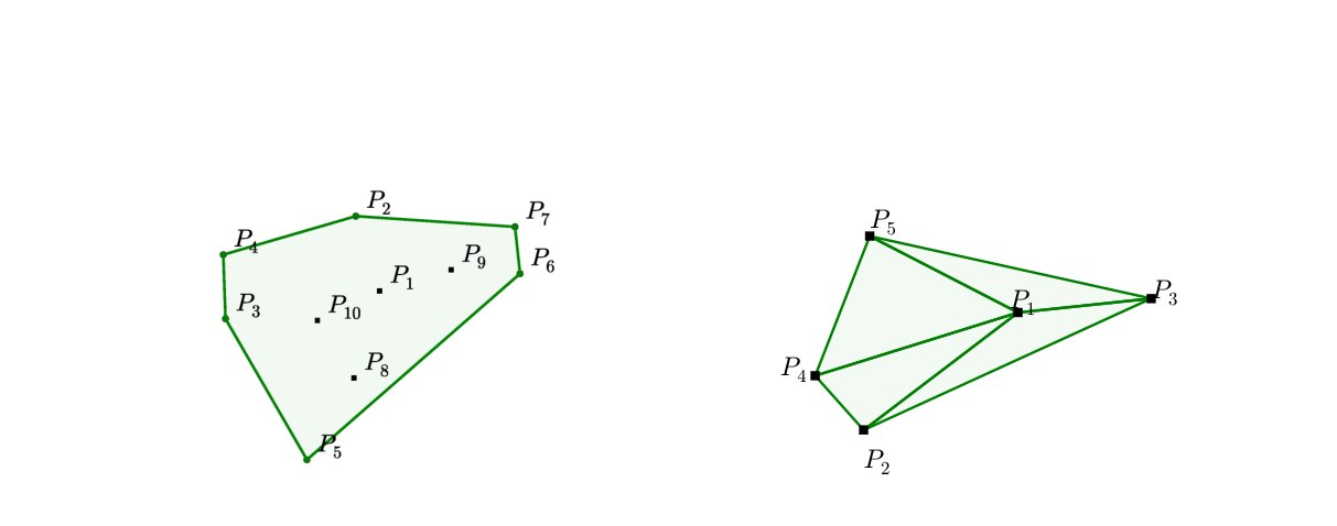
In the training data, the inputs are planar point sets $\mathcal{P}=\{P_{1},\dots,P_{n}\}$ with $n$ elements each, where $P_{j}=(x_{j},y_{j})$ are the cartesian coordinates of the points over which we find the convex hull, the Delaunay triangulation or the solution to the corresponding Travelling Salesman Problem. In all cases, we sample from a uniform distribution in $[0,1]\times[0,1]$. The outputs $\mathcal{C}^{\mathcal{P}}=\{C_{1},\dots,C_{m(\mathcal{P})}\}$ are sequences representing the solution associated to the point set $\mathcal{P}$. In Figure 2, we find an illustration of an input/output pair $(\mathcal{P},\mathcal{C}^{\mathcal{P}})$ for the convex hull and the Delaunay problems.

在训练数据中，输入是各含 $n$ 个元素的平面点集 $\mathcal{P}=\{P_{1},\dots,P_{n}\}$，其中 $P_{j}=(x_{j},y_{j})$ 是笛卡尔坐标；我们要在这些点上求凸包、Delaunay 三角剖分，或相应旅行商问题的解。所有情形下，我们都从 $[0,1]\times[0,1]$ 上的均匀分布采样。输出 $\mathcal{C}^{\mathcal{P}}=\{C_{1},\dots,C_{m(\mathcal{P})}\}$ 是表示该点集 $\mathcal{P}$ 所对应解的序列。图 2 给出了凸包与 Delaunay 问题上输入/输出对 $(\mathcal{P},\mathcal{C}^{\mathcal{P}})$ 的示意。

(a) Input $\mathcal{P}=\{P_{1},\dots,P_{10}\}$, and the output sequence $\mathcal{C}^{\mathcal{P}}=\{\Rightarrow,2,4,3,5,6,7,2,\Leftarrow\}$ representing its convex hull.

(b) Input $\mathcal{P}=\{P_{1},\dots,P_{5}\}$, and the output $\mathcal{C}^{\mathcal{P}}=\{\Rightarrow,(1,2,4),(1,4,5),(1,3,5),(1,2,3),\Leftarrow\}$ representing its Delaunay Triangulation.

Figure 2: Input/output representation for (a) convex hull and (b) Delaunay triangulation. The tokens $\Rightarrow$ and $\Leftarrow$ represent beginning and end of sequence, respectively.

(a) 输入 $\mathcal{P}=\{P_{1},\dots,P_{10}\}$，输出序列 $\mathcal{C}^{\mathcal{P}}=\{\Rightarrow,2,4,3,5,6,7,2,\Leftarrow\}$ 表示它的凸包。

(b) 输入 $\mathcal{P}=\{P_{1},\dots,P_{5}\}$，输出 $\mathcal{C}^{\mathcal{P}}=\{\Rightarrow,(1,2,4),(1,4,5),(1,3,5),(1,2,3),\Leftarrow\}$ 表示它的 Delaunay 三角剖分。

图 2：（a）凸包与（b）Delaunay 三角剖分的输入/输出表示。记号 $\Rightarrow$ 和 $\Leftarrow$ 分别表示序列开始与结束。

3.1 Convex Hull

3.1 凸包

We used this example as a baseline to develop our models and to understand the difficulty of solving combinatorial problems with data driven approaches. Finding the convex hull of a finite number of points is a well understood task in computational geometry, and there are several exact solutions available (see [13, 14, 15]). In general, finding the (generally unique) solution has complexity $O(n\log n)$, where $n$ is the number of points considered.

我们把这个例子当作基线，用来发展模型，并理解用数据驱动方法解决组合问题有多难。求有限个点的凸包是计算几何中已被充分理解的任务，并且已有若干精确算法（见 [13, 14, 15]）。一般而言，寻找（通常唯一的）解的复杂度是 $O(n\log n)$，其中 $n$ 是所考虑的点数。

The vectors $\mathcal{P}_{j}$ are uniformly sampled from $[0,1]\times[0,1]$. The elements $C_{i}$ are indices between 1 and $n$ corresponding to positions in the sequence $\mathcal{P}$, or special tokens representing beginning or end of sequence. See Figure 2 (a) for an illustration. To represent the output as a sequence, we start from the point with the lowest index, and go counter-clockwise – this is an arbitrary choice but helps reducing ambiguities during training.

向量 $\mathcal{P}_{j}$ 从 $[0,1]\times[0,1]$ 中均匀采样。元素 $C_{i}$ 是介于 1 与 $n$ 之间的下标，对应于序列 $\mathcal{P}$ 中的位置，或者表示序列开始或结束的特殊记号。示意见图 2 (a)。为了把输出表示成序列，我们从下标最小的点出发，沿逆时针方向行进——这是一种任意选择，但有助于在训练时减少歧义。

3.2 Delaunay Triangulation

3.2 Delaunay 三角剖分

A Delaunay triangulation for a set $\mathcal{P}$ of points in a plane is a triangulation such that each circumcircle of every triangle is empty, that is, there is no point from $\mathcal{P}$ in its interior. Exact $O(n\log n)$ solutions are available [16], where $n$ is the number of points in $\mathcal{P}$.

平面点集 $\mathcal{P}$ 的 Delaunay 三角剖分是这样一种剖分：每个三角形的外接圆都是空的，也就是说其内部不含 $\mathcal{P}$ 中的任何点。已有精确的 $O(n\log n)$ 算法 [16]，其中 $n$ 是 $\mathcal{P}$ 中的点数。

In this example, the outputs $\mathcal{C}^{\mathcal{P}}=\{C_{1},\dots,C_{m(\mathcal{P})}\}$ are the corresponding sequences representing the triangulation of the point set $\mathcal{P}$ . Each $C_{i}$ is a triple of integers from 1 to $n$ corresponding to the position of triangle vertices in $\mathcal{P}$ or the beginning/end of sequence tokens. See Figure 2 (b).

在这个例子中，输出 $\mathcal{C}^{\mathcal{P}}=\{C_{1},\dots,C_{m(\mathcal{P})}\}$ 是表示点集 $\mathcal{P}$ 之三角剖分的相应序列。每个 $C_{i}$ 是由 1 到 $n$ 的三个整数组成的三元组，对应于 $\mathcal{P}$ 中三角形顶点的位置，或者是序列开始/结束记号。参见图 2 (b)。

We note that any permutation of the sequence $\mathcal{C}^{\mathcal{P}}$ represents the same triangulation for $\mathcal{P}$, additionally each triangle representation $C_{i}$ of three integers can also be permuted. Without loss of generality, and similarly to what we did for convex hulls at training time, we order the triangles $C_{i}$ by their incenter coordinates (lexicographic order) and choose the increasing triangle representation[^2]. Without ordering, the models learned were not as good, and finding a better ordering that the Ptr-Net could better exploit is part of future work.

我们注意到，序列 $\mathcal{C}^{\mathcal{P}}$ 的任意排列都表示 $\mathcal{P}$ 的同一份三角剖分；此外，每个由三个整数组成的三角形表示 $C_{i}$ 本身也可以排列。在不损失一般性的前提下，并与我们在训练凸包时的做法类似，我们按内心坐标（字典序）对三角形 $C_{i}$ 排序，并选择递增的三角形表示[^2]（我们取 $C_{i}=(1,2,4)$ 而非 $(2,4,1)$ 或其他排列）。如果不排序，学到的模型就没有那么好；寻找一种 Ptr-Net 能更好利用的排序，属于后续工作。

3.3 Travelling Salesman Problem (TSP)

3.3 旅行商问题（TSP）

TSP arises in many areas of theoretical computer science and is an important algorithm used for microchip design or DNA sequencing. In our work we focused on the planar symmetric TSP: given a list of cities, we wish to find the shortest possible route that visits each city exactly once and returns to the starting point. Additionally, we assume the distance between two cities is the same in each opposite direction. This is an NP-hard problem which allows us to test the capabilities and limitations of our model.

TSP 出现在理论计算机科学的许多领域，也是用于芯片设计或 DNA 测序的重要算法。本工作关注平面对称 TSP：给定一份城市列表，我们希望找到一条尽可能短的路线，恰好经过每座城市一次并回到起点。此外，我们假定两座城市之间两个方向上的距离相同。这是一个 NP 难问题，使我们能够检验模型的能力与局限。

The input/output pairs $(\mathcal{P},\mathcal{C}^{\mathcal{P}})$ have a similar format as in the Convex Hull problem described in Section 3.1. $\mathcal{P}$ will be the cartesian coordinates representing the cities, which are chosen randomly in the $[0,1]\times[0,1]$ square. $\mathcal{C}^{\mathcal{P}}=\{C_{1},\dots,C_{n}\}$ will be a permutation of integers from 1 to $n$ representing the optimal path (or tour). For consistency, in the training dataset, we always start in the first city without loss of generality.

输入/输出对 $(\mathcal{P},\mathcal{C}^{\mathcal{P}})$ 的格式与第 3.1 节所述凸包问题类似。$\mathcal{P}$ 是表示各个城市的笛卡尔坐标，在 $[0,1]\times[0,1]$ 正方形内随机选取。$\mathcal{C}^{\mathcal{P}}=\{C_{1},\dots,C_{n}\}$ 是 1 到 $n$ 的一个排列，表示最优路径（或回路）。为保持一致，在训练数据集中我们总是从第一座城市出发，这并不损失一般性。

To generate exact data, we implemented the Held-Karp algorithm [17] which finds the optimal solution in $O(2^{n}n^{2})$ (we used it up to $n=20$). For larger $n$, producing exact solutions is extremely costly, therefore we also considered algorithms that produce approximated solutions: A1 [18] and A2 [19], which are both $O(n^{2})$, and A3 [20] which implements the $O(n^{3})$ Christofides algorithm. The latter algorithm is guaranteed to find a solution within a factor of 1.5 from the optimal length. Table 2 shows how they performed in our test sets.

为生成精确数据，我们实现了 Held-Karp 算法 [17]，它在 $O(2^{n}n^{2})$ 时间内找到最优解（我们把它用到 $n=20$）。对更大的 $n$，产生精确解极其昂贵，因此我们也考虑了产生近似解的算法：A1 [18] 与 A2 [19] 的复杂度都是 $O(n^{2})$，A3 [20] 则实现了 $O(n^{3})$ 的 Christofides 算法。后一算法保证找到的解其长度不超过最优长度的 1.5 倍。表 2 给出了它们在我们测试集上的表现。

4 Empirical Results

4 实证结果

4.1 Architecture and Hyperparameters

4.1 结构与超参数

No extensive architecture or hyperparameter search of the Ptr-Net was done in the work presented here, and we used virtually the same architecture throughout all the experiments and datasets. Even though there are likely some gains to be obtained by tuning the model, we felt that having the same model hyperparameters operate on all the problems would make the main message of the paper stronger.

在本文报告的工作中，我们没有对 Ptr-Net 做广泛的结构或超参数搜索，几乎在所有实验和数据集上都使用同一套结构。尽管调参很可能还有收益，但我们觉得让同一组模型超参数应对所有问题，会使论文的主要信息更有说服力。

As a result, all our models used a single layer LSTM with either 256 or 512 hidden units, trained with stochastic gradient descent with a learning rate of 1.0, batch size of 128, random uniform weight initialization from -0.08 to 0.08, and L2 gradient clipping of 2.0. We generated 1M training example pairs, and we did observe overfitting in some cases where the task was simpler (i.e., for small $n$).

因此，我们所有模型都使用单层 LSTM，隐单元数为 256 或 512；用随机梯度下降训练，学习率为 1.0，batch 大小为 128，权重从 -0.08 到 0.08 均匀随机初始化，并对梯度做 2.0 的 L2 裁剪。我们生成了 100 万对训练样本；在任务较简单的情形（也就是 $n$ 较小）下，我们确实观察到了过拟合。

4.2 Convex Hull

4.2 凸包

We used the convex hull as the guiding task which allowed us to understand the deficiencies of standard models such as the sequence-to-sequence approach, and also setting up our expectations on what a purely data driven model would be able to achieve with respect to an exact solution.

我们把凸包当作引导任务，借此理解序列到序列等标准模型的不足，并设定我们对纯数据驱动模型相对于精确解能够达到何种程度的预期。

We reported two metrics: accuracy, and area covered of the true convex hull (note that any simple polygon will have full intersection with the true convex hull). To compute the accuracy, we considered two output sequences $\mathcal{C}^{1}$ and $\mathcal{C}^{2}$ to be the same if they represent the same polygon. For simplicity, we only computed the area coverage for the test examples in which the output represents a simple polygon (i.e., without self-intersections). If an algorithm fails to produce a simple polygon in more than 1% of the cases, we simply reported FAIL.

我们报告两项指标：准确率，以及对真实凸包的面积覆盖（注意，任何简单多边形都会与真实凸包完全相交）。计算准确率时，如果两个输出序列 $\mathcal{C}^{1}$ 和 $\mathcal{C}^{2}$ 表示同一个多边形，我们就视它们相同。为简单起见，我们只对输出表示简单多边形（也就是没有自交）的测试样本计算面积覆盖。如果某种算法在超过 1% 的情形中无法产生简单多边形，我们就直接记为 FAIL。

The results are presented in Table 1. We note that the area coverage achieved with the Ptr-Net is close to 100%. Looking at examples of mistakes, we see that most problems come from points that are aligned (see Figure 3 (d) for a mistake for $n=500$) – this is a common source of errors in most algorithms to solve the convex hull.

结果见表 1。我们注意到，Ptr-Net 达到的面积覆盖接近 100%。查看出错的例子可以看到，大多数问题来自近乎共线的点（见图 3 (d) 中 $n=500$ 时的一处错误）——这在大多数求凸包的算法中也是常见的误差来源。

It was seen that the order in which the inputs are presented to the encoder during inference affects its performance. When the points on the true convex hull are seen “late” in the input sequence, the accuracy is lower. This is possibly the network does not have enough processing steps to “update” the convex hull it computed until the latest points were seen. In order to overcome this problem, we used the attention mechanism described in Section 2.2, which allows the decoder to look at the whole input at any time. This modification boosted the model performance significantly. We inspected what attention was focusing on, and we observed that it was “pointing” at the correct answer on the input side. This inspired us to create the Ptr-Net model described in Section 2.3.

我们看到，推断时输入呈现给编码器的顺序会影响其表现。当真实凸包上的点在输入序列中出现得“较晚”时，准确率更低。这可能是因为在看到最晚的那些点之前，网络没有足够的处理步数去“更新”它已经算出的凸包。为克服这一问题，我们使用了第 2.2 节描述的注意力机制，使解码器在任意时刻都能查看全部输入。这一修改显著提升了模型表现。我们检查了注意力所聚焦的位置，观察到它正在输入一侧“指向”正确答案。这启发我们提出了第 2.3 节描述的 Ptr-Net 模型。

More than outperforming both the LSTM and the LSTM with attention, our model has the key advantage of being inherently variable length. The bottom half of Table 1 shows that, when training our model on a variety of lengths ranging from 5 to 50 (uniformly sampled, as we found other forms of curriculum learning to not be effective), a single model is able to perform quite well on all lengths it has been trained on (but some degradation for $n=50$ can be observed w.r.t. the model trained only on length 50 instances). More impressive is the fact that the model does extrapolate to lengths that it has never seen during training. Even for $n=500$, our results are satisfactory and indirectly indicate that the model has learned more than a simple lookup. Neither LSTM or LSTM with attention can be used for any given $n^{\prime}\neq n$ without training a new model on $n^{\prime}$.

我们的模型不仅优于 LSTM 以及带注意力的 LSTM，其关键优势还在于它天然支持可变长度。表 1 的下半部分表明：当我们在 5 到 50 的多种长度上训练模型（长度均匀采样，因为我们发现其他形式的课程学习并不有效）时，同一个模型在它所训练过的所有长度上都表现相当好（不过相对于只在长度 50 的实例上训练的模型，$n=50$ 时仍可看到一些下降）。更令人印象深刻的是，该模型还能外推到训练时从未见过的长度。即便对 $n=500$，我们的结果也令人满意，并间接表明模型学到的不只是简单查表。LSTM 或带注意力的 LSTM 都无法在不针对 $n^{\prime}$ 重新训练的情况下，用于任意给定的 $n^{\prime}\neq n$。

Method	trained $n$	$n$	Accuracy	Area
LSTM [1]	50	50	1.9%	FAIL
+attention [5]	50	50	38.9%	99.7%
Ptr-Net	50	50	72.6%	99.9%
LSTM [1]	5	5	87.7%	99.6%
Ptr-Net	5-50	5	92.0%	99.6%
LSTM [1]	10	10	29.9%	FAIL
Ptr-Net	5-50	10	87.0%	99.8%
Ptr-Net	5-50	50	69.6%	99.9%
Ptr-Net	5-50	100	50.3%	99.9%
Ptr-Net	5-50	200	22.1%	99.9%
Ptr-Net	5-50	500	1.3%	99.2%

Table 1: Comparison between LSTM, LSTM with attention, and our Ptr-Net model on the convex hull problem. Note that the baselines must be trained on the same $n$ that they are tested on.

方法	训练 $n$	$n$	准确率	面积
LSTM [1]	50	50	1.9%	FAIL
+attention [5]	50	50	38.9%	99.7%
Ptr-Net	50	50	72.6%	99.9%
LSTM [1]	5	5	87.7%	99.6%
Ptr-Net	5-50	5	92.0%	99.6%
LSTM [1]	10	10	29.9%	FAIL
Ptr-Net	5-50	10	87.0%	99.8%
Ptr-Net	5-50	50	69.6%	99.9%
Ptr-Net	5-50	100	50.3%	99.9%
Ptr-Net	5-50	200	22.1%	99.9%
Ptr-Net	5-50	500	1.3%	99.2%

表 1：LSTM、带注意力的 LSTM 与我们的 Ptr-Net 在凸包问题上的比较。注意，基线必须在与测试相同的 $n$ 上训练。

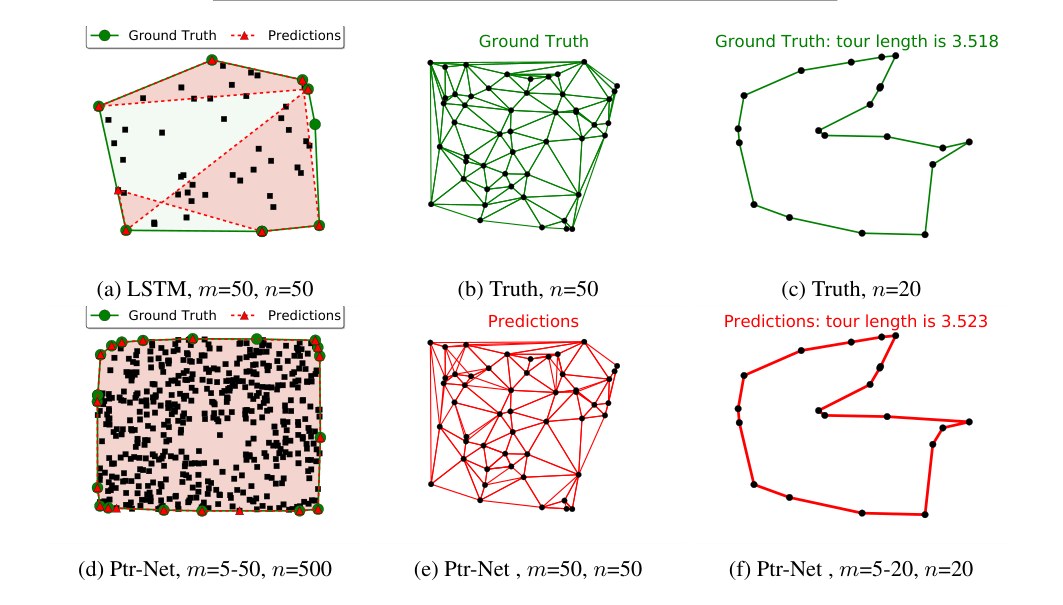
Figure 3: Examples of our model on Convex hulls (left), Delaunay (center) and TSP (right), trained on $m$ points, and tested on $n$ points. A failure of the LSTM sequence-to-sequence model for Convex hulls is shown in (a). Note that the baselines cannot be applied to a different length from training.

图 3：我们的模型在凸包（左）、Delaunay（中）和 TSP（右）上的例子，在 $m$ 个点上训练，在 $n$ 个点上测试。(a) 展示了 LSTM 序列到序列模型在凸包上的一次失败。注意，基线不能直接用到与训练不同的长度上。

4.3 Delaunay Triangulation

4.3 Delaunay 三角剖分

The Delaunay Triangulation test case is connected to our first problem of finding the convex hull. In fact, the Delaunay Triangulation for a given set of points triangulates the convex hull of these points.

Delaunay 三角剖分这一测试情形与我们的第一个问题——求凸包——是相连的。事实上，给定点集的 Delaunay 三角剖分，正是对这些点之凸包的三角剖分。

We reported two metrics: accuracy and triangle coverage in percentage (the percentage of triangles the model predicted correctly). Note that, in this case, for an input point set $\mathcal{P}$, the output sequence $\mathcal{C}(\mathcal{P})$ is, in fact, a set. As a consequence, any permutation of its elements will represent the same triangulation.

我们报告两项指标：准确率，以及以百分比表示的三角形覆盖（模型正确预测的三角形所占比例）。注意，在这种情形下，对于输入点集 $\mathcal{P}$，输出序列 $\mathcal{C}(\mathcal{P})$ 实际上是一个集合。因此，其元素的任意排列都表示同一份三角剖分。

Using the Ptr-Net model for $n=5$, we obtained an accuracy of 80.7% and triangle coverage of 93.0%. For $n=10$, the accuracy was 22.6% and the triangle coverage 81.3%. For $n=50$, we did not produce any precisely correct triangulation, but obtained 52.8% triangle coverage. See the middle column of Figure 3 for an example for $n=50$.

使用 Ptr-Net，在 $n=5$ 时我们得到 80.7% 的准确率和 93.0% 的三角形覆盖。在 $n=10$ 时，准确率为 22.6%，三角形覆盖为 81.3%。在 $n=50$ 时，我们没有产生任何完全正确的三角剖分，但得到了 52.8% 的三角形覆盖。图 3 中间一列给出了 $n=50$ 时的一个例子。

4.4 Travelling Salesman Problem

4.4 旅行商问题

We considered the planar symmetric travelling salesman problem (TSP), which is NP-hard as the third problem. Similarly to finding convex hulls, it also has sequential outputs. Given that the Ptr-Net implements an $O(n^{2})$ algorithm, it was unclear if it would have enough capacity to learn a useful algorithm solely from data.

我们把平面对称旅行商问题（TSP）作为第三个问题来考虑，它是 NP 难的。与求凸包类似，它的输出也是序列。鉴于 Ptr-Net 实现的是 $O(n^{2})$ 算法，事先并不清楚它是否有足够容量，仅从数据中就学到一个有用的算法。

As discussed in Section 3.3, it is feasible to generate exact solutions for relatively small values of $n$ to be used as training data. For larger $n$, due to the importance of TSP, good and efficient algorithms providing reasonable approximate solutions exist. We used three different algorithms in our experiments – A1, A2, and A3 (see Section 3.3 for references).

如第 3.3 节所述，对相对较小的 $n$ 生成用作训练数据的精确解是可行的。对更大的 $n$，由于 TSP 很重要，已有一些良好且高效、能给出合理近似解的算法。我们在实验中使用了三种不同的算法——A1、A2 和 A3（参考文献见第 3.3 节）。

Table 2 shows all of our results on TSP. The number reported is the length of the proposed tour. Unlike the convex hull and Delaunay triangulation cases, where the decoder was unconstrained, in this example we set the beam search procedure to only consider valid tours. Otherwise, the Ptr-Net model would sometimes output an invalid tour – for instance, it would repeat two cities or decided to ignore a destination. This procedure was relevant for $n>20$, where at least 10% of instances would not produce any valid tour.

表 2 给出了我们在 TSP 上的全部结果。所报告的数字是所提出回路的长度。与凸包和 Delaunay 三角剖分的情形不同——那里解码器不受约束——在本实验中我们把束搜索过程设为只考虑合法回路。否则，Ptr-Net 有时会输出不合法的回路，例如重复两座城市，或决定忽略某个目的地。这一步骤对 $n>20$ 是重要的，因为那时至少 10% 的实例会产生不出任何合法回路。

The first group of rows in the table show the Ptr-Net trained on optimal data, except for $n=50$, since that is not feasible computationally (we trained a separate model for each $n$). Interestingly, when using the worst algorithm (A1) data to train the Ptr-Net, our model outperforms the algorithm that is trying to imitate.

表中第一组行展示了在最优数据上训练的 Ptr-Net，但 $n=50$ 除外，因为那时在计算上不可行（我们对每个 $n$ 训练了单独的模型）。有意思的是，当用最差算法（A1）的数据来训练 Ptr-Net 时，我们的模型超过了它试图模仿的那种算法。

The second group of rows in the table show how the Ptr-Net trained on optimal data with 5 to 20 cities can generalize beyond that. The results are virtually perfect for $n=25$, and good for $n=30$, but it seems to break for 40 and beyond (still, the results are far better than chance). This contrasts with the convex hull case, where we were able to generalize by a factor of 10. However, the underlying algorithms are of far greater complexity than $O(n\log n)$, which could explain this phenomenon.

表中第二组行展示了在 5 到 20 座城市的最优数据上训练的 Ptr-Net 如何向外推广。结果在 $n=25$ 时几乎完美，在 $n=30$ 时仍然不错，但到 40 及以上似乎就失效了（尽管结果仍远好于随机）。这与凸包的情形形成对照，那里我们能够按 10 倍外推。不过，其底层算法的复杂度远高于 $O(n\log n)$，这或许可以解释这一现象。

$n$	Optimal	A1	A2	A3	Ptr-Net
5	2.12	2.18	2.12	2.12	2.12
10	2.87	3.07	2.87	2.87	2.88
50 (A1 trained)	N/A	6.46	5.84	5.79	6.42
50 (A3 trained)	N/A	6.46	5.84	5.79	6.09
5 (5-20 trained)	2.12	2.18	2.12	2.12	2.12
10 (5-20 trained)	2.87	3.07	2.87	2.87	2.87
20 (5-20 trained)	3.83	4.24	3.86	3.85	3.88
25 (5-20 trained)	N/A	4.71	4.27	4.24	4.30
30 (5-20 trained)	N/A	5.11	4.63	4.60	4.72
40 (5-20 trained)	N/A	5.82	5.27	5.23	5.91
50 (5-20 trained)	N/A	6.46	5.84	5.79	7.66

Table 2: Tour length of the Ptr-Net and a collection of algorithms on a small scale TSP problem.

$n$	最优	A1	A2	A3	Ptr-Net
5	2.12	2.18	2.12	2.12	2.12
10	2.87	3.07	2.87	2.87	2.88
50 (A1 trained)	N/A	6.46	5.84	5.79	6.42
50 (A3 trained)	N/A	6.46	5.84	5.79	6.09
5 (5-20 trained)	2.12	2.18	2.12	2.12	2.12
10 (5-20 trained)	2.87	3.07	2.87	2.87	2.87
20 (5-20 trained)	3.83	4.24	3.86	3.85	3.88
25 (5-20 trained)	N/A	4.71	4.27	4.24	4.30
30 (5-20 trained)	N/A	5.11	4.63	4.60	4.72
40 (5-20 trained)	N/A	5.82	5.27	5.23	5.91
50 (5-20 trained)	N/A	6.46	5.84	5.79	7.66

表 2：Ptr-Net 与一组算法在小规模 TSP 问题上的回路长度。

5 Conclusions

5 结论

In this paper we described Ptr-Net, a new architecture that allows us to learn a conditional probability of one sequence $\mathcal{C}^{\mathcal{P}}$ given another sequence $\mathcal{P}$, where $\mathcal{C}^{\mathcal{P}}$ is a sequence of discrete tokens corresponding to positions in $\mathcal{P}$. We show that Ptr-Nets can be used to learn solutions to three different combinatorial optimization problems. Our method works on variable sized inputs (yielding variable sized output dictionaries), something the baseline models (sequence-to-sequence with or without attention) cannot do directly. Even more impressively, they outperform the baselines on fixed input size problems - to which both the models can be applied.

在本文中，我们描述了 Ptr-Net，这是一种新结构，使我们能够学习在给定序列 $\mathcal{P}$ 的条件下另一个序列 $\mathcal{C}^{\mathcal{P}}$ 的条件概率，其中 $\mathcal{C}^{\mathcal{P}}$ 是对应于 $\mathcal{P}$ 中若干位置的离散记号序列。我们表明，Ptr-Net 可用来学习三个不同组合优化问题的解。我们的方法适用于可变大小的输入（从而产生可变大小的输出词典），这是基线模型（带或不带注意力的序列到序列）无法直接做到的。更令人印象深刻的是，它们在固定输入大小的问题上也超过了基线——而这两类模型都可以应用于这类问题。

Previous methods such as RNNSearch, Memory Networks and Neural Turing Machines [5, 6, 2] have used attention mechanisms to process inputs. However these methods do not directly address problems that arise with variable output dictionaries. We have shown that an attention mechanism can be applied to the output to solve such problems. In so doing, we have opened up a new class of problems to which neural networks can be applied without artificial assumptions. In this paper, we have applied this extension to RNNSearch, but the methods are equally applicable to Memory Networks and Neural Turing Machines.

以往的方法，如 RNNSearch、记忆网络（Memory Networks）和神经图灵机 [5, 6, 2]，已经用注意力机制来处理输入。不过这些方法并不直接处理可变输出词典所带来的问题。我们已经表明，可以把注意力机制用到输出上，以解决这类问题。这样一来，我们为神经网络打开了一类新问题，使其不必再依赖人为设定的假设。在本文中，我们把这一扩展用到了 RNNSearch 上，但这些方法同样适用于记忆网络和神经图灵机。

Future work will try and show its applicability to other problems such as sorting where the outputs are chosen from the inputs. We are also excited about the possibility of using this approach to other combinatorial optimization problems.

后续工作将尝试展示它在其他问题上的适用性，例如输出选自输入的排序。我们也期待把这一思路用到其他组合优化问题上。

Acknowledgments

We would like to thank Rafal Jozefowicz, Ilya Sutskever, Quoc Le and Samy Bengio for useful discussions on this topic. We would also like to thank Daniel Gillick for his help with the final manuscript.

致谢

我们感谢 Rafal Jozefowicz、Ilya Sutskever、Quoc Le 和 Samy Bengio 就本主题进行的有益讨论。我们也感谢 Daniel Gillick 对最终稿的帮助。

References

参考文献

[1] Ilya Sutskever, Oriol Vinyals, and Quoc V Le. Sequence to sequence learning with neural networks. In Advances in Neural Information Processing Systems , pages 3104–3112, 2014.

[2] Alex Graves, Greg Wayne, and Ivo Danihelka. Neural turing machines. arXiv preprint arXiv:1410.5401 , 2014.

[3] David E Rumelhart, Geoffrey E Hinton, and Ronald J Williams. Learning internal representations by error propagation. Technical report, DTIC Document, 1985.

[4] Anthony J Robinson. An application of recurrent nets to phone probability estimation. Neural Networks, IEEE Transactions on , 5(2):298–305, 1994.

[5] Dzmitry Bahdanau, Kyunghyun Cho, and Yoshua Bengio. Neural machine translation by jointly learning to align and translate. In ICLR 2015, arXiv preprint arXiv:1409.0473 , 2014.

[6] Jason Weston, Sumit Chopra, and Antoine Bordes. Memory networks. In ICLEAR 2015, arXiv preprint arXiv:1410.3916 , 2014.

[7] Oriol Vinyals, Lukasz Kaiser, Terry Koo, Slav Petrov, Ilya Sutskever, and Geoffrey Hinton. Grammar as a foreign language. arXiv preprint arXiv:1412.7449 , 2014.

[8] Oriol Vinyals, Alexander Toshev, Samy Bengio, and Dumitru Erhan. Show and tell: A neural image caption generator. In CVPR 2015, arXiv preprint arXiv:1411.4555 , 2014.

[9] Jeff Donahue, Lisa Anne Hendricks, Sergio Guadarrama, Marcus Rohrbach, Subhashini Venugopalan, Kate Saenko, and Trevor Darrell. Long-term recurrent convolutional networks for visual recognition and description. In CVPR 2015, arXiv preprint arXiv:1411.4389 , 2014.

[10] Wojciech Zaremba and Ilya Sutskever. Learning to execute. arXiv preprint arXiv:1410.4615 , 2014.

[11] Sepp Hochreiter and Jürgen Schmidhuber. Long short-term memory. Neural computation , 9(8):1735–1780, 1997.

[12] Nitish Srivastava, Elman Mansimov, and Ruslan Salakhutdinov. Unsupervised learning of video representations using lstms. In ICML 2015, arXiv preprint arXiv:1502.04681 , 2015.

[13] Ray A Jarvis. On the identification of the convex hull of a finite set of points in the plane. Information Processing Letters , 2(1):18–21, 1973.

[14] Ronald L. Graham. An efficient algorith for determining the convex hull of a finite planar set. Information processing letters , 1(4):132–133, 1972.

[15] Franco P. Preparata and Se June Hong. Convex hulls of finite sets of points in two and three dimensions. Communications of the ACM , 20(2):87–93, 1977.

[16] S1 Rebay. Efficient unstructured mesh generation by means of delaunay triangulation and bowyer-watson algorithm. Journal of computational physics , 106(1):125–138, 1993.

[17] Richard Bellman. Dynamic programming treatment of the travelling salesman problem. Journal of the ACM (JACM) , 9(1):61–63, 1962.

[18] Suboptimal travelling salesman problem (tsp) solver, 2015. Available at https://github.com/dmishin/tsp-solver.

[19] Traveling salesman problem c++ implementation, 2015. Available at https://github.com/samlbest/traveling-salesman.

[20] C++ implementation of traveling salesman problem using christofides and 2-opt, 2015. Available at https://github.com/beckysag/traveling-salesman.