PlantTraitNet: An Uncertainty-Aware Multimodal Framework for Global-Scale Plant Trait Inference from Citizen Science Data
PlantTraitNet: An Uncertainty-Aware Multimodal Framework for Global-Scale Plant Trait Inference from Citizen Science Data
PlantTraitNet:面向全球尺度植物性状推断的不确定性感知多模态框架,数据来自公民科学
PlantTraitNet: An Uncertainty-Aware Multimodal Framework for Global-Scale Plant Trait Inference from Citizen Science Data
Ayushi Sharma Johanna Trost Daniel Lusk Johannes Dollinger Julian Schrader Christian Rossi Javier Lopatin Etienne Laliberté Simon Haberstroh Jana Eichel Daniel Mederer Jose Miguel Cerda-Paredes Shyam S. Phartyal Lisa-Maricia Schwarz Anja Linstädter Maria Conceição Caldeira Teja Kattenborn
Abstract
摘要
Global plant maps of plant traits, such as leaf nitrogen or plant height, are essential for understanding ecosystem processes, including the carbon and energy cycles of the Earth system. However, existing trait maps remain limited by the high cost and sparse geographic coverage of field-based measurements. Citizen science initiatives offer a largely untapped resource to overcome these limitations, with over 50 million geotagged plant photographs worldwide capturing valuable visual information on plant morphology and physiology. In this study, we introduce PlantTraitNet, a multi-modal, multi-task uncertainty-aware deep learning framework that predicts four key plant traits (plant height, leaf area, specific leaf area, and nitrogen content) from citizen science photos using weak supervision. By aggregating individual trait predictions across space, we generate global maps of trait distributions. We validate these maps against independent vegetation survey data (sPlotOpen) and benchmark them against leading global trait products. Our results show that PlantTraitNet consistently outperforms existing trait maps across all evaluated traits, demonstrating that citizen science imagery, when integrated with computer vision and geospatial AI, enables not only scalable but also more accurate global trait mapping. This approach offers a powerful new pathway for ecological research and Earth system modeling.
叶氮或株高等植物性状的全球图,对理解生态系统过程至关重要,包括地球系统中的碳循环和能量循环。不过,现有性状图仍受限于实地测量成本高、地理覆盖稀疏。公民科学计划提供了尚未被充分利用的资源来克服这些限制:全球超过 5000 万张带地理标签的植物照片,捕捉了关于植物形态和生理的宝贵视觉信息。本研究介绍 PlantTraitNet,一个多模态、多任务、具备不确定性感知的深度学习框架,它在弱监督下从公民科学照片预测四项关键植物性状(株高、叶面积、比叶面积和氮含量)。通过在空间上聚合单个性状预测,我们生成性状分布的全球图。我们用独立的植被调查数据(sPlotOpen)验证这些图,并与领先的全球性状产品进行比较。结果表明,PlantTraitNet 在所有评估性状上都持续超过已有性状图,说明公民科学影像一旦与计算机视觉和地理空间人工智能结合,不仅可扩展,也能更准确地绘制全球性状。这一方法为生态研究和地球系统建模提供了一条有力的新路径。
1Chair of Sensor-based Geoinformatics, University of Freiburg, Germany
2EcoVision Lab, DM3L, University of Zurich, Switzerland
3Department of Biological Sciences, Macquarie University, Australia
4Swiss National Park, Switzerland
5Facultad de Ingeniería y Ciencias, Universidad Adolfo Ibáñez, Chile
6Department of Biological Sciences, Université de Montréal, Canada
7Chair of Ecosystem Physiology, University of Freiburg, Germany
8Department of Physical Geography, Utrecht University, The Netherlands
9Institute for Earth System Science and Remote Sensing, Leipzig University, Germany
10Data Observatory, Universidad Adolfo Ibáñez, Chile
11Department of Forestry, Mizoram University, India
12Biodiversity Research / Systematic Botany, University of Potsdam, Germany
13Department of Plant Nutrition, Institute of Crop Science and Resource Conservation, University of Bonn, Germany
14Forest Research Centre, School of Agriculture, University of Lisbon, Portugal
ayushi.sharma@geosense.uni-freiburg.de, teja.kattenborn@geosense.uni-freiburg.de
Code — github.com/GeoSense-Freiburg/PlantTraitNet
代码 — github.com/GeoSense-Freiburg/PlantTraitNet
Datasets — huggingface.co/datasets/ayushi3536/PlantTraitNet
数据集 — huggingface.co/datasets/ayushi3536/PlantTraitNet
Extended version — https://arxiv.org/abs/2511.06943
Introduction
引言
Terrestrial plants, as the largest primary producers on Earth, contribute about 60% to the global net primary productivity (Field et al. 1998) and play a critical role in the carbon and energy cycles of our Earth system (Pan et al. 2011; Schlesinger and Bernhardt 2020). However, understanding how plants influence these cycles is challenging, as the functioning of plants varies profoundly according to their traits. For instance, traits such as canopy height and leaf area control resource acquisition, while leaf tissue properties, such as nitrogen content or dry matter content, are indicators of plant resilience (Díaz et al. 2016). Although these traits are essential for understanding ecosystem processes, the data on such traits is sparse, as their measurement involves costly field surveys and laboratory analysis. Global plant trait databases such as TRY (Kattge et al. 2011) aggregate thousands of trait measurements from numerous studies and regions, providing an invaluable resource for functional biogeography and ecosystem modeling. However, even with these collective efforts, significant gaps persist in the geographic coverage of trait data across biomes, ecosystems, and species, constraining our ability to fully understand and predict global patterns of vegetation function and change (Díaz et al. 2016; Kattge et al. 2020).
陆地植物作为地球上最大的初级生产者,贡献了全球净初级生产力的约 60%(Field et al. 1998),并在地球系统的碳循环和能量循环中扮演关键角色(Pan et al. 2011; Schlesinger and Bernhardt 2020)。不过,理解植物如何影响这些循环并不容易,因为植物的功能会随其性状深刻变化。例如,冠层高度和叶面积控制资源获取,而叶组织属性,如氮含量或干物质含量,则是植物恢复力的指标(Díaz et al. 2016)。尽管这些性状对理解生态系统过程至关重要,相关数据仍然稀疏,因为测量涉及昂贵的野外调查和实验室分析。TRY 等全球植物性状数据库(Kattge et al. 2011)汇集了来自众多研究和地区的数千条性状测量,为功能生物地理学和生态系统建模提供了宝贵资源。即便有这些集体努力,性状数据在生物群系、生态系统和物种上的地理覆盖仍有显著空白,限制了我们充分理解和预测植被功能与变化的全球格局的能力(Díaz et al. 2016; Kattge et al. 2020)。
Given the strong link between plant morphology and function, plant photographs in concert with computer vision offer a promising avenue for large-scale estimation of plant traits. Citizen science platforms such as iNaturalist (Su and Maji 2021) and Pl@ntNet (Garcin et al. 2021) have collected more than 50 million research-grade plant photographs around the world, creating a unique resource for uncovering global plant trait distributions (Wolf et al. 2022). These datasets, primarily curated for the identification of plant species, provide plant images and species labels, but do not provide trait annotations (Goëau et al. 2025; Stevens et al. 2024; Van Horn et al. 2018). However, prior work has demonstrated that trait information for these species can be indirectly obtained by linking species names from citizen science records to trait databases such as TRY (Schiller et al. 2021; Wolf et al. 2022). Through this species-level matching, trait values can be weakly assigned to images, enabling the construction of large-scale, trait-annotated image datasets. These datasets can then be used to train scalable computer vision models for trait prediction from images (Schiller et al. 2021). Such models enable direct trait estimation from photographs, independent of whether the species is known or if a record exists in a trait database. Here, we attempt to advance this approach by predicting multiple traits simultaneously, leveraging shared visual features and underlying trait correlations. Subsequently, we spatially aggregate trait predictions derived from individual geotagged photographs to create global, gridded geospatial maps representing the trait distributions across plant communities and ecosystems (Schiller et al. 2021).
鉴于植物形态与功能之间的紧密联系,植物照片与计算机视觉相结合,为大规模估计植物性状提供了一条有前景的路径。iNaturalist(Su and Maji 2021)和 Pl@ntNet(Garcin et al. 2021)等公民科学平台已经在全球收集了超过 5000 万张研究级植物照片,成为揭示全球植物性状分布的独特资源(Wolf et al. 2022)。这些数据集主要为植物物种识别而整理,提供植物图像和物种标签,但不提供性状标注(Goëau et al. 2025; Stevens et al. 2024; Van Horn et al. 2018)。不过,先前工作已经表明,可以通过把公民科学记录中的物种名与 TRY 等性状数据库关联,间接获得这些物种的性状信息(Schiller et al. 2021; Wolf et al. 2022)。通过这种物种级匹配,可以把性状值弱分配给图像,从而构建大规模、带性状标注的图像数据集。这些数据集随后可用来训练可扩展的计算机视觉模型,从图像预测性状(Schiller et al. 2021)。这类模型能够直接从照片估计性状,而不依赖物种是否已知、或性状库中是否已有记录。在此,我们试图推进这一路线:同时预测多项性状,利用共享的视觉特征和底层的性状相关性。随后,我们把来自单张带地理标签照片的性状预测在空间上聚合,生成表示植物群落和生态系统性状分布的全球网格化地理空间图(Schiller et al. 2021)。
The geolocation of each photograph not only enables the spatial aggregation of the predictions into geospatial maps but also allows for the integration of spatial context into the prediction process itself (Schiller et al. 2021). For instance, climate, including temperature and precipitation, or phenological information from satellite data is known to be the key variable shaping global trait distributions, making it a promising predictor (Bruelheide et al. 2018; Schiller et al. 2021; Joswig et al. 2022). However, integrating large-scale geospatial products can be challenging due to data gaps and feature selection (Lusk et al. 2025).
每张照片的地理位置不仅使预测能够聚合为地理空间图,也允许把空间上下文融入预测过程本身(Schiller et al. 2021)。例如,包括温度和降水在内的气候,或来自卫星数据的物候信息,已知是塑造全球性状分布的关键变量,因此是有前景的预测因子(Bruelheide et al. 2018; Schiller et al. 2021; Joswig et al. 2022)。不过,整合大规模地理空间产品可能面临数据缺口和特征选择的挑战(Lusk et al. 2025)。
Recent advances in geospatial foundation models (GeoFMs) now support the seamless integration of such context into downstream tasks. Examples include Climplicit (Dollinger et al. 2025), which encodes climate information, and SatCLIP (Klemmer et al. 2025), which leverages satellite Earth observation data. Such GeoFMs have demonstrated strong generalization in global mapping applications. In this study, we test the integration of such GeoFMs into visual trait prediction to enhance performance through geospatial context.
地理空间基础模型(GeoFMs)的近期进展,现在支持把这类上下文无缝纳入下游任务。例子包括编码气候信息的 Climplicit(Dollinger et al. 2025),以及利用卫星地球观测数据的 SatCLIP(Klemmer et al. 2025)。这类 GeoFM 已在全球制图应用中展现出很强的泛化能力。在本研究中,我们检验把这类 GeoFM 融入视觉性状预测,通过地理空间上下文提升性能。
An important challenge for computer vision with citizen science data is its inherent heterogeneity and noise (Sierra et al. 2024), ranging from inconsistent image quality due to varied photo acquisition methods (feature noise) to ambiguous trait annotations from weak supervision (label noise). Such data characteristics may result in implausible predictions and leave an imprint on the aggregation into global trait products. Moreover, such training data noise can substantially degrade a model’s ability to generalize to unseen data (Lu and He 2022; Arpit et al. 2017; Zhang et al. 2021). To overcome both feature and label noise in the citizen-science data, we propose an uncertainty-aware probabilistic deep learning framework that estimates predictive uncertainty. The predicted uncertainty is used to dynamically down-weight highly noisy samples and to filter out unreliable data points, thereby reducing overfitting to spurious patterns.
公民科学数据用于计算机视觉时的一项重要挑战,是其固有的异质性和噪声(Sierra et al. 2024),既包括拍照方式不一带来的图像质量不一致(特征噪声),也包括弱监督带来的模糊性状标注(标签噪声)。这类数据特征可能导致不合理的预测,并在聚合成全球性状产品时留下痕迹。此外,这类训练数据噪声会显著削弱模型对未见数据的泛化能力(Lu and He 2022; Arpit et al. 2017; Zhang et al. 2021)。为同时克服公民科学数据中的特征噪声和标签噪声,我们提出一个会估计预测不确定性的不确定性感知概率深度学习框架。预测不确定性被用来动态下调高噪声样本的权重,并过滤不可靠的数据点,从而减少对虚假模式的过拟合。
Overall, our contributions are summarized as follows:
总体而言,我们的贡献概括如下:
- • We introduce the first machine learning–ready dataset that systematically links crowd-sourced plant photographs from citizen science platforms to species-level trait values derived from global trait databases.
- • 我们介绍第一个面向机器学习、系统地把来自公民科学平台的众包植物照片与来自全球性状数据库的物种级性状值关联起来的数据集。
- • We present PlantTraitNet, the first uncertainty-aware, multimodal, multi-task deep learning model for global-scale prediction of four key plant traits: height (H), leaf area (LA), specific leaf area (SLA), and leaf nitrogen content (LN).
- • 我们提出 PlantTraitNet,第一个面向全球尺度预测四项关键植物性状的不确定性感知、多模态、多任务深度学习模型:株高(H)、叶面积(LA)、比叶面积(SLA)和叶氮含量(LN)。
- • We apply PlantTraitNet on more than 300K independent samples of citizen science photos and spatially aggregate the predictions to global trait maps. A benchmark against globally distributed vegetation survey data (sPlotOpen) revealed that these PlantTraitNet-derived traits maps consistently outperform previous global trait products.
- • 我们在超过 30 万张独立的公民科学照片上应用 PlantTraitNet,并把预测在空间上聚合成全球性状图。与全球分布的植被调查数据(sPlotOpen)比较表明,这些由 PlantTraitNet 得到的性状图持续超过先前的全球性状产品。
Data
数据
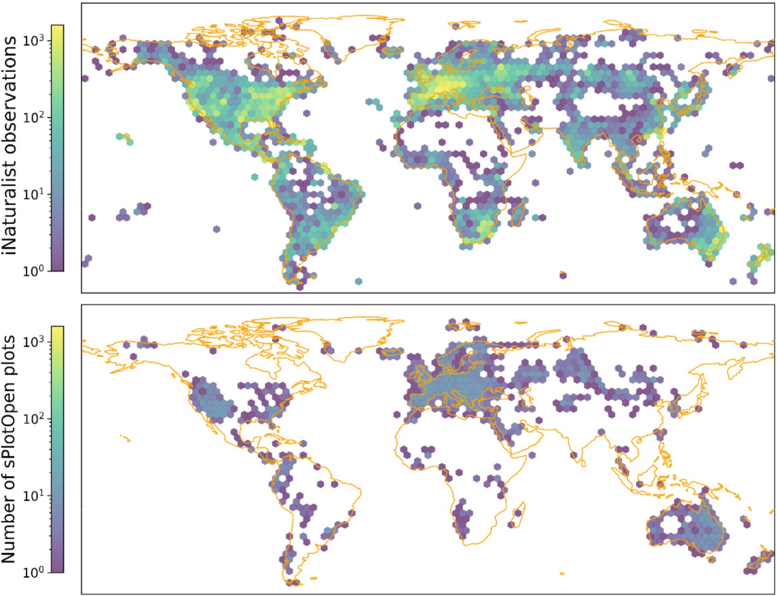
Figure 1: Geographic coverage of the citizen science data (top) and independent benchmark reference data (bottom) from vegetation surveys (Sabatini et al. 2021, sPlotOpen,).
图 1:公民科学数据的地理覆盖(上)以及来自植被调查的独立基准参考数据(下)(Sabatini et al. 2021,sPlotOpen)。
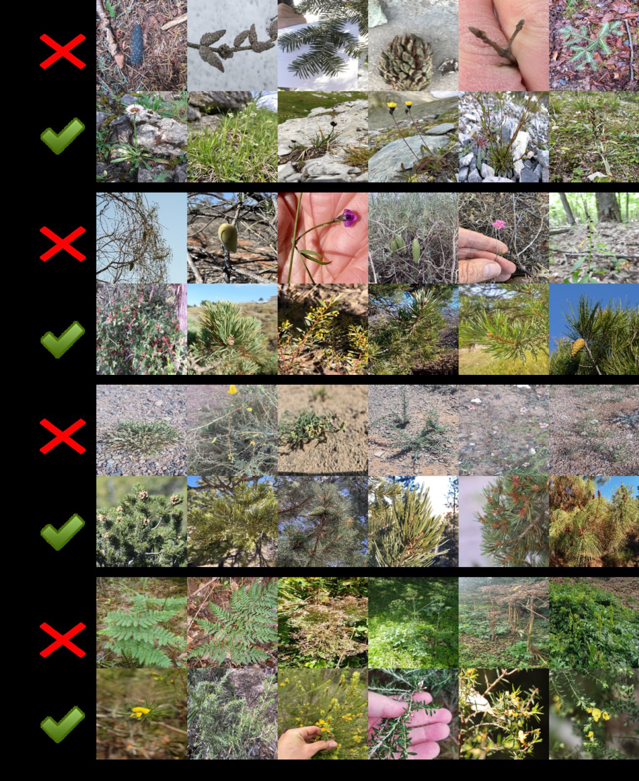
Figure 2: Randomly sampled images showing highest/lowest predictive uncertainty (see Methodology). Observations: Height uncertainty often from unsuitable contexts (winter scenes, fruits, hands). SLA uncertainty from images lacking visible leaves (bare branches, flowers, buds). Leaf Nitrogen: low-quality/blurry images. Leaf Area: exotic leaf types (e.g., ferns).
图 2:随机采样的图像,展示最高/最低的预测不确定性(见方法)。观察:株高不确定性常常来自不合适的情境(冬季景象、果实、手)。SLA 不确定性来自看不见叶子的图像(光秃枝条、花、芽)。叶氮:低质量/模糊图像。叶面积:少见叶型(例如蕨类)。
Weakly Labeled Citizen Science Photographs
弱标注的公民科学照片
To predict plant traits at a global scale, we utilize two large-scale citizen science datasets: iNaturalist (GBIF.org 2025; Su and Maji 2021) and Pl@ntNet-300K (Garcin et al. 2021). These datasets consist of plant images annotated with species labels and geolocations but lack direct trait measurements. Following Schiller et al. (2021), we weakly annotate each image using species-level trait distributions from the TRY database (Kattge et al. 2020), based on the premise that interspecific trait variation (variation between species) generally exceeds intraspecific variation (variation within species) (Dong et al. 2020; Wright et al. 2017).
为了在全球尺度预测植物性状,我们使用两个大规模公民科学数据集:iNaturalist(GBIF.org 2025; Su and Maji 2021)和 Pl@ntNet-300K(Garcin et al. 2021)。这些数据集由带有物种标签和地理位置的植物图像组成,但缺少直接的性状测量。沿循 Schiller et al.(2021),我们使用来自 TRY 数据库(Kattge et al. 2020)的物种级性状分布对每张图像做弱标注,其前提是种间性状变异(物种之间的变异)通常超过种内变异(物种内部的变异)(Dong et al. 2020; Wright et al. 2017)。
We model each trait as a normal distribution per species, using TRY-derived means and standard deviations, and sample trait values within the interquartile range to reduce outlier influence. To account for intraspecific variability, we resample traits for each image at every training epoch (Schiller et al. 2021).
我们把每个性状按物种建模为正态分布,使用来自 TRY 的均值和标准差,并在四分位距内采样性状值,以减少离群点的影响。为了考虑种内变异性,我们在每个训练轮次为每张图像重新抽样性状(Schiller et al. 2021)。
This weak supervision introduces label noise, especially for traits with strong intraspecies variability across developmental stages (e.g., juvenile trees assigned mature height).
这种弱监督会引入标签噪声,对那些随发育阶段有很强种内变异的性状尤其明显(例如,幼树被赋予成年株高)。
We further reduce noise through model-driven uncertainty estimates (see Methodology). The final dataset includes approximately 220K training images across 5K species and over 80K images in the validation set.
我们进一步通过模型驱动的不确定性估计来降低噪声(见方法)。最终数据集包含约 22 万张训练图像,覆盖 5000 个物种,验证集中有超过 8 万张图像。
Vegetation Survey Data - sPlotOpen
植被调查数据:sPlotOpen
For evaluation, we use the sPlotOpen database (Sabatini et al. 2021). The georeferenced sPlotOpen records represent plant community compositions, which were linked with trait data from the TRY database (Kattge et al. 2020). This data provides global trait maps of community-weighted mean (CWM) trait values.
为了评估,我们使用 sPlotOpen 数据库(Sabatini et al. 2021)。带地理参考的 sPlotOpen 记录表示植物群落组成,并与来自 TRY 数据库(Kattge et al. 2020)的性状数据关联。这些数据提供群落加权平均(CWM)性状值的全球性状图。
Reference Data
参考数据
To aid uncertainty-based filtering, we curated a small dataset of 780 species with images and trait measurements taken from the same individual at the same time including observations from diverse regions such as Germany, La Palma, India, Australia etc. (See Appendix for details)
为辅助基于不确定性的过滤,我们整理了一个约 780 个物种的小型数据集,其中图像和性状测量来自同一个体、同一时刻,观测覆盖德国、拉帕尔马、印度、澳大利亚等多样地区(细节见附录)。
Methodology
方法
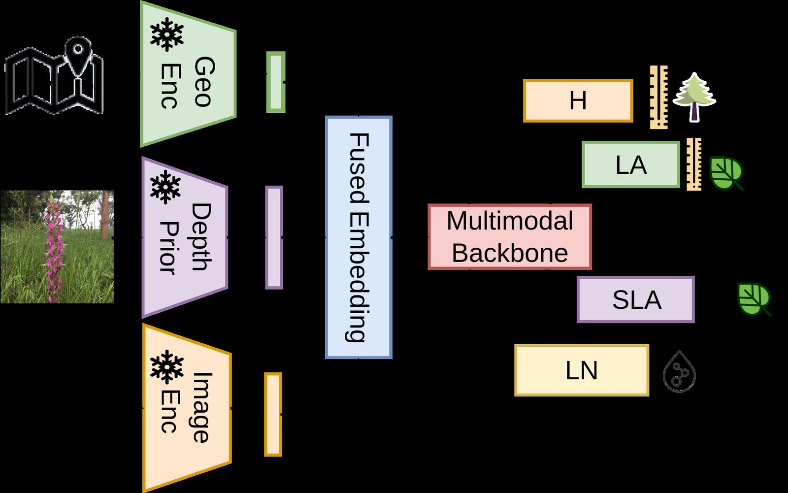
Figure 3: The model integrates image, depth, and geospatial embeddings. These are fused within a multimodal backbone, which then uses individual heads to predict height (H), leaf area (LA), specific leaf area (SLA), and leaf nitrogen (LN).
图 3:模型整合图像、深度和地理空间嵌入。它们在多模态主干中融合,随后用各自的头预测株高(H)、叶面积(LA)、比叶面积(SLA)和叶氮(LN)。
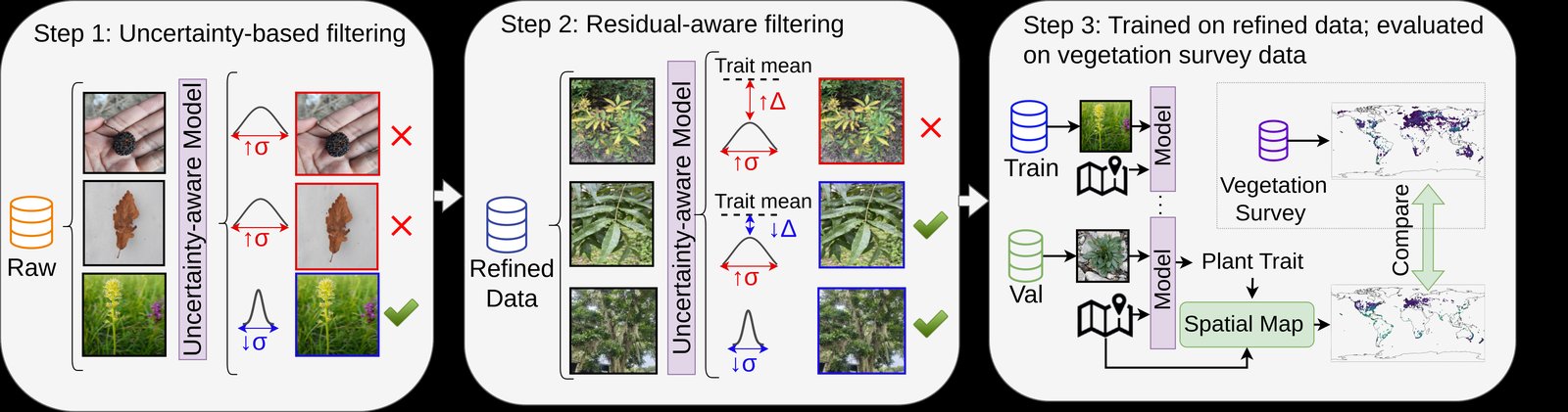
Figure 4: Overview of the pipeline. We filter weakly labeled citizen science data (Raw data) based on high model uncertainty (Step 1) and large residuals from species trait medians (Step 2). We use this refined data for training the models (Step 3), which are evaluated by comparing spatially aggregated predictions (1° resolution) against overlapping vegetation surveys (sPlotOpen).
图 4:流程概览。我们根据高模型不确定性(步骤 1)以及相对物种性状中位数的大残差(步骤 2)过滤弱标注的公民科学数据(原始数据)。我们用清洗后的数据训练模型(步骤 3),并通过把空间聚合预测(1° 分辨率)与重叠的植被调查(sPlotOpen)比较来评估。
The PlantTraitNet architecture (Fig. 3), uses a general-purpose vision encoder. In addition to image features, we incorporate depth and geospatial priors. These modality-specific embeddings are fused using simple concatenation. The fused representation is passed through a shared multimodal backbone, followed by trait-specific linear heads.
PlantTraitNet 架构(图 3)使用通用视觉编码器。除图像特征外,我们还纳入深度和地理空间先验。这些模态特定的嵌入通过简单拼接融合。融合表示经过共享的多模态主干,再接到性状特定的线性头。
Image Encoder
图像编码器
Given an input image , we use the pretrained DINOv2 ViT-B/14 encoder to extract a sequence of patch-level feature embeddings (Oquab et al. 2023).
给定输入图像 ,我们使用预训练的 DINOv2 ViT-B/14 编码器提取一组 patch 级特征嵌入 (Oquab et al. 2023)。
We apply adaptive average pooling along the patch tokens , reducing it to a 32-dimensional representation. This pooling operation is parameter-free and preserves condensed spatial structure before projection. This pooled output is flattened and passed through a multi-layer perceptron (MLP) to generate the embedding of dimension 768.
我们沿 patch token 维 做自适应平均池化,将其压缩为 32 维表示。这一池化操作没有参数,并在投影前保留浓缩后的空间结构。池化输出被展平后送入多层感知机(MLP),生成维数为 768 的嵌入。
Depth Priors from Foundation Models
来自基础模型的深度先验
A novel addition to our architecture is the use of depth priors from foundation models for monocular depth estimation. While standard 2D RGB images lack explicit three-dimensional spatial cues, depth information encodes the distance between the sensor and surface points on the plant, enabling a more accurate reconstruction of plant morphology and structure. To incorporate depth, we use the pretrained and frozen encoder from the Depth-Anything-V2 (DA-V2) model (Yang et al. 2024), denoted as . Although various models could be used, we adopt DA-V2 for its strong generalization capabilities, attributed to its training on large-scale labeled and unlabeled datasets and its student-teacher distillation framework. We use the ViT-B variant, which outputs a set of embeddings . Similar to the image encoder, we apply adaptive average pooling along the patch token dimension , reducing it to a 64-dimensional representation. This pooled output is flattened and passed through a MLP to generate the depth prior embedding of dimension 768.
我们架构中的一项新加入,是使用来自单目深度估计基础模型的深度先验。标准二维 RGB 图像缺少显式的三维空间线索,而深度信息编码传感器与植物表面点之间的距离,从而能够更准确地重建植物形态和结构。为了纳入深度,我们使用 Depth-Anything-V2(DA-V2)模型中预训练并冻结的编码器(Yang et al. 2024),记为 。虽然可以使用多种模型,我们选择 DA-V2 是因为它泛化能力强,这得益于它在大规模有标注和无标注数据上的训练,以及学生–教师蒸馏框架。我们使用 ViT-B 变体,它输出一组嵌入 。与图像编码器类似,我们沿 patch token 维 做自适应平均池化,将其压缩为 64 维表示。池化输出被展平后送入 MLP,生成维数为 768 的深度先验嵌入。
Geospatial Priors from Foundation Models
来自基础模型的地理空间先验
Plants are tailored to local climatic conditions, such as precipitation and temperature, through their traits (Joswig et al. 2022).
植物通过其性状适应局地气候条件,例如降水和温度(Joswig et al. 2022)。
To incorporate this climatic context as a cue in the prediction process, we integrate Climplicit (Dollinger et al. 2025) into our architecture, a spatio-temporal geo-location encoder trained on the CHELSA climate dataset (Karger et al. 2017). Climplicit maps latitude, longitude, and month of the year to a continuous embedding that implicitly captures climatic factors such as temperature and precipitation. To incorporate seasonal trends, we concatenate the embeddings for the months of March, June, September, and December.
为了把这种气候上下文作为线索纳入预测过程,我们把 Climplicit(Dollinger et al. 2025)融入架构。它是一个在 CHELSA 气候数据集(Karger et al. 2017)上训练的时空地理位置编码器。Climplicit 把纬度、经度和一年中的月份映射为连续嵌入,隐式捕捉温度和降水等气候因子。为了纳入季节趋势,我们拼接三月、六月、九月和十二月的嵌入。
Multimodal and Multi-Task Backbone
多模态与多任务主干
Let denote the image embedding obtained from the pretrained DINOv2 encoder, and denote the depth embedding obtained from the DA-V2 encoder. To incorporate geospatial context, we project the 1024-dimensional embedding produced by Climplicit denoted as to a 256-dimensional vector using a trainable linear projection.
令 表示由预训练 DINOv2 编码器得到的图像嵌入, 表示由 DA-V2 编码器得到的深度嵌入。为了纳入地理空间上下文,我们用可训练的线性投影,把 Climplicit 产生的 1024 维嵌入 投影到 256 维向量。
The multimodal representation is formed by concatenating all embeddings and is then projected to a 1024-dimensional representation via a linear layer: The resulting embedding is passed through a residual network of 8 residual blocks with hidden dimension twice the embedding size. This architecture and embedding dimensions were chosen based on an ablation across multiple configurations (see Appendix). Finally, the output feature representation is passed to four independent heads for trait prediction in our multi-task architecture.
多模态表示由拼接所有嵌入形成,随后经线性层投影到 1024 维: 得到的嵌入经过由 8 个残差块组成的残差网络,隐层维度为嵌入大小的两倍。这一架构和嵌入维度是根据多种配置的消融选定的(见附录)。最后,输出特征表示被送到我们多任务架构中的四个独立头,用于性状预测。
Uncertainty Estimation
不确定性估计
To capture uncertainty in plant trait prediction, each trait-specific prediction head outputs both the predicted value and its associated uncertainty, following the method by (Jiang et al. 2024). For each trait , the model predicts two values for each sample : the mean and the log-scale parameter , where the scale or standard deviation is given by .
为了刻画植物性状预测中的不确定性,每个性状特定的预测头会同时输出预测值及其相关不确定性,做法沿循 Jiang et al.(2024)。对每个性状 ,模型为每个样本 预测两个值:均值 和对数尺度参数 ,其中尺度或标准差由 给出。
We model the predictive distribution differently for each trait based on its statistical characteristics. For Leaf Area (LA), which exhibits a long-tailed distribution, we use a Laplace distribution parameterized by mean and scale . The Laplace distribution is more suitable for modeling long-tailed distributions compared to Gaussian distributions (Jiang et al. 2024).
我们根据每个性状的统计特性,用不同方式建模预测分布。对呈长尾分布的叶面积(LA),我们使用由均值 和尺度 参数化的拉普拉斯分布。与高斯分布相比,拉普拉斯分布更适合建模长尾分布(Jiang et al. 2024)。
For the remaining traits, Height (H), Specific Leaf Area (SLA), and Leaf Nitrogen (LN), we assume a Gaussian distribution with mean and standard deviation . Although plant height has strong skewness (dominance of small plants), we employ stratified sampling based on plant functional types during training. This ensures that each mini-batch contains approximately equal representation of grasses, shrubs, and trees, which may make the Gaussian assumption more suitable for modeling this trait (respective ablations are described in the Appendix).
对其余性状,即株高(H)、比叶面积(SLA)和叶氮(LN),我们假定高斯分布,均值为 ,标准差为 。虽然株高有很强的偏斜(小植株占主导),我们在训练时按植物功能型做分层抽样。这确保每个小批量大致均衡地包含草本、灌木和乔木,可能使高斯假设更适合建模这一性状(相应消融见附录)。
Uncertainty-Guided Data Cleaning Loop
不确定性引导的数据清洗循环
Citizen science image datasets offer large-scale and diverse data for plant trait modeling but suffer from substantial noise and inconsistencies. Common issues include the presence of non-plant objects, non-representative plant parts, uninformative specimens, and scenes that are too dense, distant, or blurred (Fig. 2). Manual curation at this scale is impractical, and species-level trait annotations often ignore individual variation. Neural networks often memorize noisy labels which harms generalization and makes noise handling essential (Lu and He 2022; Arpit et al. 2017; Zhang et al. 2021). Lu and He (2022) shows models initially learn from clean samples but, past a ‘turning point’, begin memorizing noise, leading to poorer generalization.
公民科学图像数据集为植物性状建模提供了大规模、多样的数据,但也存在大量噪声和不一致。常见问题包括非植物物体、不具代表性的植物部位、信息量不足的标本,以及过于密集、过远或模糊的场景(图 2)。在这种规模上手动整理并不现实,而物种级性状标注常常忽略个体差异。神经网络常常记住嘈杂标签,这会损害泛化,因而处理噪声至关重要(Lu and He 2022; Arpit et al. 2017; Zhang et al. 2021)。Lu and He(2022)表明,模型最初从干净样本中学习,但过了“转折点”后开始记住噪声,从而导致更差的泛化。
Building on this insight, we implement a two-step data cleaning loop guided by model-predicted uncertainty (Fig. 4). The first step applies uncertainty-based filtering: after early training for a single epoch on raw data, all training images are inferred and ranked by trait-wise uncertainty, and those exceeding a joint threshold across all traits are filtered out. This process continues iteratively until the number of samples jointly flagged as uncertain across traits falls below a predefined threshold.
基于这一认识,我们实现了一个由模型预测不确定性引导的两步数据清洗循环(图 4)。第一步施加基于不确定性的过滤:在原始数据上提前训练一个 epoch 后,对所有训练图像做推断并按性状不确定性排序,超过所有性状联合阈值的样本被过滤掉。这一过程迭代进行,直到在各性状上被联合标记为不确定的样本数低于预设阈值。
However, uncertainty alone can be unreliable for heteroscedastic traits such as plant height, where variance naturally increases with trait magnitude. In such cases, high uncertainty may reflect genuine biological variability rather than label noise. Consequently, filtering solely by uncertainty risks biasing the cleaned dataset toward lower-variance samples. To mitigate this, the second stage performs residual-aware filtering, combining uncertainty and prediction residuals. For this, we identify the ‘turning point’ while training for each trait. We do so by tracking performance on the reference dataset and selecting the epoch after which trait-wise performance begins to deteriorate. Using predictions from this epoch, we calculate the mean absolute error between predicted trait values and species-level means for samples with high uncertainty. Images with high uncertainty and large residuals are filtered from the dataset. The cleaning loop terminates when the number of samples satisfying the filtering criteria becomes negligible. Further details are provided in Appendix.
不过,仅靠不确定性对异方差性状(例如株高)可能并不可靠,因为方差会自然随性状量级增加。在这些情形中,高不确定性可能反映真实的生物学变异,而不是标签噪声。因此,只按不确定性过滤,有可能使清洗后的数据集偏向低方差样本。为减轻这一点,第二阶段进行残差感知过滤,把不确定性和预测残差结合起来。为此,我们在每个性状的训练过程中识别“转折点”。我们通过跟踪参考数据集上的表现,选择性状表现开始变差之后的那个 epoch。使用该 epoch 的预测,我们计算高不确定性样本的预测性状值与物种级均值之间的平均绝对误差。同时具有高不确定性和大残差的图像会从数据集中被过滤掉。当满足过滤准则的样本数变得可以忽略时,清洗循环终止。更多细节见附录。
Model Evaluation and Selection
模型评估与选择
Following the approach of previous studies (Wolf et al. 2022; Dechant et al. 2024), we aggregated the plot-level trait values from sPlotOpen to a 1-degree spatial resolution to generate a global benchmark dataset. We then applied PlantTraitNet to predict trait values using more than 300K globally distributed citizen science observations. The predicted trait values were aggregated to the same 1-degree resolution and filtered to include only grid cells with at least 20 observations, resulting in over 890 grid cells. To ensure a robust and interpretable evaluation, we used complementary metrics that capture different aspects of model performance: the coefficient of determination (R²) quantifies the proportion of variance in observed trait values explained by the predictions, the normalized mean absolute error (nMAE) measures the average deviation normalized by the observed trait range, and Pearson’s correlation coefficient (r) on log-transformed values quantifies the linear relationship between predicted and observed data. To account for spatial sampling bias, all metrics are weighted by the area of each 1-degree grid cell. We also compare previously published trait maps against the same sPlotOpen CWM values on overlapping grid cells (Boonman et al. 2020; Butler et al. 2017; Madani et al. 2018; Moreno-Martínez et al. 2018; Schiller et al. 2021; Van Bodegom et al. 2014; Wolf et al. 2022). For the ablation study, all models were assessed solely on our validation dataset.
沿循先前研究的做法(Wolf et al. 2022; Dechant et al. 2024),我们把 sPlotOpen 的样方级性状值聚合到 1 度空间分辨率,以生成全球基准数据集。随后我们用 PlantTraitNet 对超过 30 万条全球分布的公民科学观测预测性状值。预测性状值被聚合到相同的 1 度分辨率,并过滤为只包含至少 20 条观测的网格单元,最终得到超过 890 个网格单元。为了保证评估稳健、可解释,我们使用捕捉模型表现不同方面的互补指标:决定系数(R²)量化观测性状值方差中由预测解释的比例;归一化平均绝对误差(nMAE)衡量按观测性状范围归一化后的平均偏差;在对数变换值上的皮尔逊相关系数(r)量化预测与观测之间的线性关系。为考虑空间采样偏差,所有指标都按每个 1 度网格单元的面积加权。我们还把先前发表的性状图与同一套 sPlotOpen CWM 值在重叠网格单元上进行比较(Boonman et al. 2020; Butler et al. 2017; Madani et al. 2018; Moreno-Martínez et al. 2018; Schiller et al. 2021; Van Bodegom et al. 2014; Wolf et al. 2022)。对消融研究,所有模型仅在我们的验证数据集上评估。
The final model, with approximately 90M trainable parameters, was trained for up to 30 epochs with a batch size of 256 on a single NVIDIA RTX A6000 GPU (using approximately 20 GB VRAM). To select the optimal model checkpoint across all traits, we compute the Pareto front using the Non-Dominated Sorting (NDS) algorithm (Deb et al. 2002). We then calculate the hypervolume for all candidate checkpoints on this front (Zitzler et al. 2001) and select the checkpoint that maximizes the hypervolume. Following Lacoste et al. (2019), we estimate a total of 93.86 kg CO2 emissions for all experiments across seeds. This estimate excludes testing and failed runs and therefore likely underestimates the total emissions, but it provides a reasonable guideline for future model training.
最终模型约有 9000 万可训练参数,在单张 NVIDIA RTX A6000 GPU 上以批量大小 256 训练最多 30 个 epoch(大约使用 20 GB 显存)。为了在所有性状上选择最优模型检查点,我们用非支配排序(NDS)算法(Deb et al. 2002)计算帕累托前沿。随后我们计算该前沿上所有候选检查点的超体积(Zitzler et al. 2001),并选择使超体积最大的检查点。沿循 Lacoste et al.(2019),我们估计所有跨随机种子实验的总排放为 93.86 千克二氧化碳。这一估计排除了测试和失败运行,因此可能低估总排放,但它为未来模型训练提供了合理参考。
Results
结果
| Method | Metric | H | LA | SLA | LN |
|---|---|---|---|---|---|
| Ours | ↑ | 0.19 | 0.30 | 0.23 | -0.16 |
| (Raw) | nMAE ↓ | 0.22 | 0.14 | 0.14 | 0.17 |
| ↑ | 0.45 | 0.56 | 0.59 | 0.49 | |
| Ours | ↑ | 0.18 | 0.34 | 0.27 | -0.12 |
| (Refined) | nMAE ↓ | 0.22 | 0.14 | 0.13 | 0.17 |
| ↑ | 0.45 | 0.57 | 0.59 | 0.50 | |
| Schiller | ↑ | -0.32 | 0.11 | 0.16 | 0.06 |
| nMAE ↓ | 0.28 | 0.17 | 0.14 | 0.14 | |
| ↑ | 0.42 | 0.52 | 0.53 | 0.40 | |
| Wolf | ↑ | -0.61 | -0.02 | 0.02 | -0.20 |
| nMAE ↓ | 0.31 | 0.18 | 0.16 | 0.18 | |
| ↑ | 0.43 | 0.53 | 0.50 | 0.41 | |
| Moreno | ↑ | – | – | -0.72 | -0.85 |
| nMAE ↓ | – | – | 0.23 | 0.22 | |
| ↑ | – | – | 0.23 | 0.17 | |
| Butler | ↑ | – | – | -0.17 | -0.50 |
| nMAE ↓ | – | – | 0.18 | 0.20 | |
| ↑ | – | – | 0.29 | 0.32 | |
| Boonman | ↑ | – | – | 0.03 | -0.37 |
| nMAE ↓ | – | – | 0.16 | 0.18 | |
| ↑ | – | – | 0.49 | 0.20 | |
| Madani | ↑ | – | – | -0.76 | – |
| nMAE ↓ | – | – | 0.23 | – | |
| ↑ | – | – | -0.07 | – | |
| Bodegom | ↑ | – | – | -1.00 | – |
| nMAE ↓ | – | – | 0.24 | – | |
| ↑ | – | – | 0.33 | – |
Table 1: Global trait map benchmarking against sPlotOpen CWMs (1° resolution). Best. Second-best. External products: Schiller (Schiller et al. 2021), Wolf (Wolf et al. 2022), Moreno (Moreno-Martínez et al. 2018), Butler (Butler et al. 2017), Boonman (Boonman et al. 2020), Madani (Madani et al. 2018), Bodegom (Van Bodegom et al. 2014). PlantTraitNet (Ours) is evaluated after training on both raw and refined datasets.
| 方法 | 指标 | H | LA | SLA | LN |
|---|---|---|---|---|---|
| 本文 | ↑ | 0.19 | 0.30 | 0.23 | -0.16 |
| (原始) | nMAE ↓ | 0.22 | 0.14 | 0.14 | 0.17 |
| ↑ | 0.45 | 0.56 | 0.59 | 0.49 | |
| 本文 | ↑ | 0.18 | 0.34 | 0.27 | -0.12 |
| (清洗后) | nMAE ↓ | 0.22 | 0.14 | 0.13 | 0.17 |
| ↑ | 0.45 | 0.57 | 0.59 | 0.50 | |
| Schiller | ↑ | -0.32 | 0.11 | 0.16 | 0.06 |
| nMAE ↓ | 0.28 | 0.17 | 0.14 | 0.14 | |
| ↑ | 0.42 | 0.52 | 0.53 | 0.40 | |
| Wolf | ↑ | -0.61 | -0.02 | 0.02 | -0.20 |
| nMAE ↓ | 0.31 | 0.18 | 0.16 | 0.18 | |
| ↑ | 0.43 | 0.53 | 0.50 | 0.41 | |
| Moreno | ↑ | – | – | -0.72 | -0.85 |
| nMAE ↓ | – | – | 0.23 | 0.22 | |
| ↑ | – | – | 0.23 | 0.17 | |
| Butler | ↑ | – | – | -0.17 | -0.50 |
| nMAE ↓ | – | – | 0.18 | 0.20 | |
| ↑ | – | – | 0.29 | 0.32 | |
| Boonman | ↑ | – | – | 0.03 | -0.37 |
| nMAE ↓ | – | – | 0.16 | 0.18 | |
| ↑ | – | – | 0.49 | 0.20 | |
| Madani | ↑ | – | – | -0.76 | – |
| nMAE ↓ | – | – | 0.23 | – | |
| ↑ | – | – | -0.07 | – | |
| Bodegom | ↑ | – | – | -1.00 | – |
| nMAE ↓ | – | – | 0.24 | – | |
| ↑ | – | – | 0.33 | – |
表 1:全球性状图相对 sPlotOpen 群落加权平均(1° 分辨率)的基准比较。最优。次优。外部产品:Schiller(Schiller et al. 2021)、Wolf(Wolf et al. 2022)、Moreno(Moreno-Martínez et al. 2018)、Butler(Butler et al. 2017)、Boonman(Boonman et al. 2020)、Madani(Madani et al. 2018)、Bodegom(Van Bodegom et al. 2014)。PlantTraitNet(本文)在原始数据和清洗后数据上训练后分别评估。
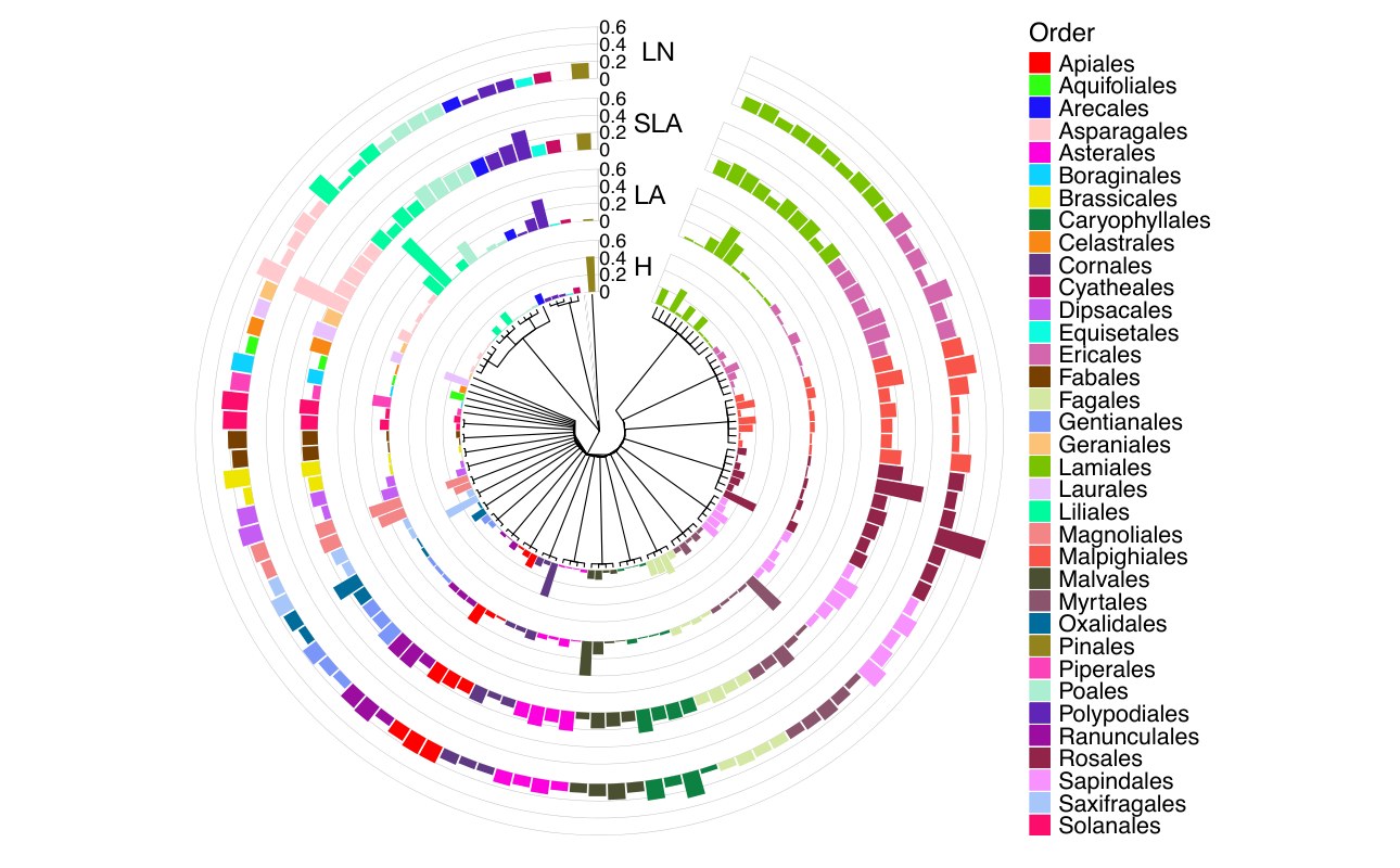
Figure 5: Mean relative prediction error (MRPE) computed on validation data at the family level, visualized along the taxonomic tree, for height (H), leaf area (LA), specific leaf area (SLA) and leaf nitrogen (LN).
图 5:在验证数据上按科计算的平均相对预测误差(MRPE),沿分类树可视化,分别对应株高(H)、叶面积(LA)、比叶面积(SLA)和叶氮(LN)。
| Image | Geo | Depth | H | LA | SLA | LN | # Top ranks | |
|---|---|---|---|---|---|---|---|---|
| Multi-Task | DinoV2 | ✗ | ✗ | 0.15 ± 0.00 | 0.31 ± 0.00 | 0.32 ± 0.00 | 0.14 ± 0.01 | 1 |
| BioCLIP | ✗ | ✗ | 0.15 ± 0.01 | 0.3 ± 0.00 | 0.32 ± 0.01 | 0.15 ± 0.04 | 1 | |
| DinoV2 | SatCLIP | ✗ | 0.16 ± 0.02 | 0.27 ± 0.04 | 0.25 ± 0.02 | 0.11 ± 0.05 | 0 | |
| DinoV2 | GeoCLIP | ✗ | 0.17 ± 0.01 | 0.33 ± 0.01 | 0.32 ± 0.00 | 0.15 ± 0.02 | 3 | |
| DinoV2 | Climplicit | ✗ | 0.19 ± 0.01 | 0.32 ± 0.01 | 0.31 ± 0.01 | 0.16 ± 0.06 | 3 | |
| BioCLIP | Climplicit | ✗ | 0.19 ± 0.00 | 0.32 ± 0.02 | 0.31 ± 0.01 | 0.15 ± 0.06 | 3 | |
| BioCLIP | Climplicit | DA-V2 | 0.16 ± 0.01 | 0.28 ± 0.03 | 0.30 ± 0.00 | 0.19 ± 0.02 | 1 | |
| DinoV2 | Climplicit | DA-V2 | 0.19 ± 0.02 | 0.32 ± 0.01 | 0.31 ± 0.02 | 0.18 ± 0.05 | 4 | |
| ST | DinoV2 | Climplicit | DA-V2 | 0.12 ± 0.01 | 0.34 ± 0.01 | 0.33 ± 0.01 | 0.21 ± 0.02 | – |
Table 2: Multi-modal ablation study for plant trait prediction. Results are reported as mean 1 standard deviation over 3 runs. Bold indicates the best result, and italic indicates the second-best. ‘# Top ranks’ counts the number of top-two rankings. The last row reports the performance of the best multi-task model when evaluated in a single-task (ST) setting.
| 图像 | 地理 | 深度 | H | LA | SLA | LN | 进入前两名的次数 | |
|---|---|---|---|---|---|---|---|---|
| 多任务 | DinoV2 | ✗ | ✗ | 0.15 ± 0.00 | 0.31 ± 0.00 | 0.32 ± 0.00 | 0.14 ± 0.01 | 1 |
| BioCLIP | ✗ | ✗ | 0.15 ± 0.01 | 0.3 ± 0.00 | 0.32 ± 0.01 | 0.15 ± 0.04 | 1 | |
| DinoV2 | SatCLIP | ✗ | 0.16 ± 0.02 | 0.27 ± 0.04 | 0.25 ± 0.02 | 0.11 ± 0.05 | 0 | |
| DinoV2 | GeoCLIP | ✗ | 0.17 ± 0.01 | 0.33 ± 0.01 | 0.32 ± 0.00 | 0.15 ± 0.02 | 3 | |
| DinoV2 | Climplicit | ✗ | 0.19 ± 0.01 | 0.32 ± 0.01 | 0.31 ± 0.01 | 0.16 ± 0.06 | 3 | |
| BioCLIP | Climplicit | ✗ | 0.19 ± 0.00 | 0.32 ± 0.02 | 0.31 ± 0.01 | 0.15 ± 0.06 | 3 | |
| BioCLIP | Climplicit | DA-V2 | 0.16 ± 0.01 | 0.28 ± 0.03 | 0.30 ± 0.00 | 0.19 ± 0.02 | 1 | |
| DinoV2 | Climplicit | DA-V2 | 0.19 ± 0.02 | 0.32 ± 0.01 | 0.31 ± 0.02 | 0.18 ± 0.05 | 4 | |
| 单任务 | DinoV2 | Climplicit | DA-V2 | 0.12 ± 0.01 | 0.34 ± 0.01 | 0.33 ± 0.01 | 0.21 ± 0.02 | – |
表 2:植物性状预测的多模态消融研究。结果报告为 3 次运行的平均 1 个标准差。粗体表示最优结果,斜体表示次优。“进入前两名的次数”统计进入前两名的次数。最后一行报告最佳多任务模型在单任务(ST)设定下评估时的表现。
Benchmarking Against Vegetation Survey Data
相对植被调查数据的基准比较
We benchmark our global trait maps derived from models trained on both raw and filtered data and those of previous studies using R², Pearson’s , and nMAE (Table 1). Depending on the metric, our model for LN delivers comparable results with those by Schiller et al. (Schiller et al. 2021). For the other three traits, our models consistently achieve higher performance than previously published plant trait maps. The overall improvement reflects the model’s ability to capture complex and variable patterns in large-scale trait prediction. While the scores suggest that the maps capture relative differences, substantially lower R² scores indicate that PlantTraitNet maps and all other products are systematically biased (also see Appendix), underscoring the inherent challenge of revealing morphological and physiological ecosystem patterns at global scale.
我们用 R²、皮尔逊 和 nMAE,对在原始数据和过滤数据上训练得到的全球性状图,以及先前研究的产品进行基准比较(表 1)。就指标而言,我们的 LN 模型与 Schiller et al.(Schiller et al. 2021)给出的结果相当。对其余三项性状,我们的模型持续取得高于先前发表植物性状图的表现。总体改进反映了模型捕捉大规模性状预测中复杂而多变格局的能力。虽然 分数表明这些图捕捉了相对差异,明显更低的 R² 分数则表明 PlantTraitNet 的图以及所有其他产品都存在系统偏差(亦见附录),这突出了在全球尺度揭示形态和生理生态系统格局的固有困难。
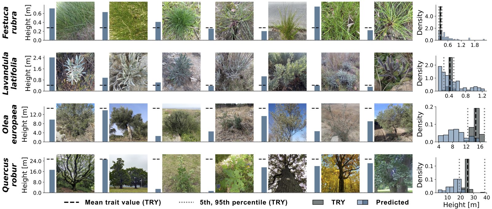
Figure 6: Intraspecific variation in predicted height for four species. Bar plots (left) show model predictions; histograms (right) show height distributions predicted from up to 100 images compared with up to 100 measurements from the TRY database.
图 6:四个物种预测株高中的种内变异。条形图(左)显示模型预测;直方图(右)显示由最多 100 张图像预测的株高分布,并与来自 TRY 数据库的最多 100 条测量比较。
Model Performance Across and Within Species
跨物种与种内的模型表现
To reveal trait variability within the biosphere on a global scale, a computer vision model must be robust across species, and thus phylogenetic lineages. Using inferences and species information from the validation data, we show that the residuals of PlantTraitNet are largely unsystematically distributed in the phylogenetic space (Fig. 5). To quantify this, we use two standard metrics of phylogenetic signal:
要在全球尺度揭示生物圈中的性状变异性,计算机视觉模型必须在物种之间、因而也在系统发育谱系之间稳健。利用验证数据中的推断和物种信息,我们表明 PlantTraitNet 的残差在系统发育空间中大体上没有系统性分布(图 5)。为了量化这一点,我们使用两项标准的系统发育信号指标:
Pagel’s , which captures broad-scale phylogenetic autocorrelation in residual covariance (Pagel 1999) and Blomberg’s , which is more sensitive to fine-scale signals among closely related species (Blomberg et al. 2003). For SLA and leaf nitrogen, the phylogenetic signal is weak ( = 0.04 and 0.15; = 0.0053 and 0.0076), suggesting that prediction errors are largely independent of species relatedness. Although errors for height ( = 0.80, = 0.018) and leaf area ( = 0.56, = 0.0067) show some phylogenetic autocorrelation, the consistently low values indicate that even closely related species do not share systematic prediction biases (see Appendix for details). Although PlantTraitNet was trained using weak annotations at the species level, these findings underscore the model’s strong generalizability and robustness across the plant tree of life.
Pagel 的 捕捉残差协方差中的大尺度系统发育自相关(Pagel 1999),Blomberg 的 则对近缘种之间的细尺度信号更敏感(Blomberg et al. 2003)。对 SLA 和叶氮,系统发育信号较弱( = 0.04 和 0.15; = 0.0053 和 0.0076),说明预测误差大体上独立于物种亲缘关系。尽管株高( = 0.80, = 0.018)和叶面积( = 0.56, = 0.0067)的误差显示出一些系统发育自相关,一贯偏低的 值表明,即便近缘种也不共享系统的预测偏差(细节见附录)。虽然 PlantTraitNet 使用物种级弱标注训练,这些发现强调了模型在植物生命之树上的强泛化能力和稳健性。
Despite weak supervision at the species level, PlantTraitNet captures within-species variability in trait expression. This is particularly evident in the case of height prediction (Fig. 6), where the model reflects differences across growth forms and developmental stages within individual species (see Appendix for additional examples of within-species variability across traits). This suggests that the model is not simply regressing to a species-level mean but is sensitive to morphological cues in the images that reflect ecological and ontogenetic variation.
尽管监督是物种级的弱监督,PlantTraitNet 仍能捕捉性状表达中的种内变异性。这在株高预测中尤其明显(图 6):模型反映了同一物种内不同生长型和发育阶段之间的差异(各性状种内变异性的更多例子见附录)。这表明模型并不仅仅回归到物种级均值,而是对图像中反映生态和个体发育变异的形态线索敏感。
Effect of Input Modalities
输入模态的影响
To evaluate the contribution of each input modality to trait prediction, we conduct an ablation study using different combinations of image, geospatial, and depth information (Table 2). Our goal is to understand how each modality influences model performance across key plant functional traits: H, LA, SLA, and LN. For this ablation study, we also experimented with a pretrained BioCLIP (Stevens et al. 2024) encoder as an alternative to DinoV2. For BioCLIP, we extracted the embedding from its classification token, as it empirically showed superior performance (detailed in the Appendix). For geospatial priors, we assess SatCLIP (Klemmer et al. 2025), which is trained on satellite imagery and captures vegetation density and phenology; GeoCLIP (Vivanco Cepeda et al. 2023), a geo-localization model trained on natural images; and Climplicit (Dollinger et al. 2025)
为了评估每种输入模态对性状预测的贡献,我们用图像、地理空间和深度信息的不同组合进行消融研究(表 2)。我们的目标是理解每种模态如何影响模型在关键植物功能性状 H、LA、SLA 和 LN 上的表现。在这项消融中,我们还试验了预训练的 BioCLIP(Stevens et al. 2024)编码器,作为 DinoV2 的替代。对 BioCLIP,我们提取其分类 token 的嵌入,因为它在经验上表现更好(详见附录)。对地理空间先验,我们评估在卫星影像上训练、捕捉植被密度和物候的 SatCLIP(Klemmer et al. 2025);在自然图像上训练的地理定位模型 GeoCLIP(Vivanco Cepeda et al. 2023);以及 Climplicit(Dollinger et al. 2025)。
We find that image features alone provide a strong baseline, with DINOv2 and BioCLIP performing comparably. Adding geospatial priors from Climplicit consistently improves performance across traits, reflected in higher R². Adding depth information on top of the image and climate input leads to marginal changes overall. In general, image features provide a strong foundation for trait inference, while the integration of climate information significantly enhances prediction. Although depth contributes selectively, its inclusion offers a modest gain in average performance, supporting the use of all three modalities in the final model.
我们发现,仅图像特征就提供了很强的基线,DINOv2 与 BioCLIP 表现相当。加入来自 Climplicit 的地理空间先验会持续提高各性状表现,体现为更高的 R²。在图像和气候输入之上再加入深度信息,总体变化不大。一般而言,图像特征为性状推断提供了坚实基础,而气候信息的整合会显著增强预测。虽然深度的贡献是选择性的,纳入它仍会给平均表现带来适度提升,从而支持在最终模型中使用全部三种模态。
Multi-Task versus Single-Task
多任务与单任务
In Table 2, we also compare the effect of jointly predicting all traits (multi-task) versus independently predicting each trait using the same architecture with single trait heads (single-task). While the single-task architecture yields marginally better performance for LA, SLA, and LN (e.g., higher and lower nMAE), the multi-task model shows a substantial performance gain for H, improving from 0.12 to 0.19. Importantly, the multi-task model achieves these results with significantly lower computational cost—training a single joint model instead of four separate ones reduces training time and GPU memory usage by approximately 75%. Thus, the multi-task model provides a better overall balance of performance and efficiency.
在表 2 中,我们还比较了联合预测所有性状(多任务)与使用相同架构、但只有单个性状头来独立预测每个性状(单任务)的效果。虽然单任务架构在 LA、SLA 和 LN 上略好(例如更高的 和更低的 nMAE),多任务模型在 H 上有大幅提升,把 从 0.12 提高到 0.19。重要的是,多任务模型以明显更低的计算成本取得这些结果:训练一个联合模型而不是四个独立模型,大约减少 75% 的训练时间和 GPU 显存占用。因此,多任务模型在表现和效率之间提供了更好的总体平衡。
Discussion
讨论
Predicting plant traits from citizen science photos is challenging due to data variability and biases, including spatial and taxonomic bias, and overrepresentation of smaller growth forms such as grasses and herbs (Di Cecco et al. 2021; Sierra et al. 2024). Ecological complexity adds difficulty, as traits vary across biomes, with generalists showing common traits and specialists distinct ones, resulting in skewed, long-tailed distributions (see Appendix). Unlike animals with fixed body plans, e.g. with symmetric and fixed numbers of legs or arms, plants have a comparably flexible morphology, resulting in varying numbers of plant organs, such as leaves or branches. This variability complicates trait prediction via computer vision. Despite these challenges, our results show promising potential. Future work should focus on reducing biases through targeted data acquisition. Increased acquisition of reference data to enable better ‘turning point’ selection and incorporate label correction to improve model robustness and generalization in ecological contexts.
从公民科学照片预测植物性状很困难,原因在于数据的变异性和偏差,包括空间和分类偏差,以及对草本和草本植物等较小生长型的过度代表(Di Cecco et al. 2021; Sierra et al. 2024)。生态复杂性增加了难度,因为性状会跨生物群系变化,广布种表现出常见性状,专化种则有独特性状,从而形成偏斜的长尾分布(见附录)。与具有固定身体构型的动物不同,例如对称且数量固定的腿或臂,植物的形态相对灵活,导致叶或分枝等植物器官数量多变。这种变异性使通过计算机视觉预测性状变得复杂。尽管有这些挑战,我们的结果仍显示出有前景的潜力。未来工作应通过有针对性的数据采集来减少偏差。增加参考数据的采集,以便更好地选择“转折点”,并纳入标签校正,从而提高模型在生态情境中的稳健性和泛化能力。
Conclusion
结论
Our understanding of plant–environment interactions is limited by the sparse geographic and taxonomic coverage of morphological and physiological trait data. We demonstrate that citizen science plant images, combined with machine learning can be used to predict and map global distributions of key ecological plant traits using only geolocated images making the approach highly scalable across biomes. Despite relying on weak supervision via species-level trait annotations, our models capture consistent intraspecific variation. Integrating geospatial context through Earth observation foundation models (GeoFMs) and structural cues via depth priors improves predictive performance and model robustness. Our multi-task framework enables simultaneous prediction of multiple traits, capturing inter-trait dependencies while improving computational efficiency. Benchmarking against existing global trait maps shows that our approach achieves state-of-the-art performance. This establishes a new baseline for large-scale trait inference from image data, offering a powerful alternative to traditional mapping based on field sampling and extrapolation. By leveraging abundant publicly available plant images, our method enables automated, global retrieval of core traits, offering new opportunities to explore functional diversity and improve ecosystem modeling under global change.
我们对植物–环境相互作用的理解,受到形态和生理性状数据在地理和分类覆盖上稀疏的限制。我们表明,公民科学植物图像与机器学习相结合,可以仅用带地理位置的图像来预测并绘制关键生态植物性状的全球分布,从而使该方法在各生物群系中高度可扩展。尽管依赖通过物种级性状标注得到的弱监督,我们的模型仍能捕捉一致的种内变异。通过地球观测基础模型(GeoFMs)整合地理空间上下文,并通过深度先验整合结构线索,提高了预测表现和模型稳健性。我们的多任务框架能够同时预测多项性状,捕捉性状之间的依赖,同时提高计算效率。与已有全球性状图的基准比较表明,我们的方法达到了当前最优水平。这为从图像数据做大规模性状推断建立了新的基线,为基于野外采样和外推的传统制图提供了有力替代。通过利用大量公开可得的植物图像,我们的方法能够自动、全球地检索核心性状,为探索功能多样性、并在全球变化下改进生态系统建模提供新的机会。
Acknowledgements
致谢
This study was funded by the German Research Foundation (DFG) within the project PANOPS (Revealing Earth’s plant functional diversity with citizen science; project no. 504978936)
本研究由德国研究基金会(DFG)在 PANOPS 项目(用公民科学揭示地球的植物功能多样性;项目号 504978936)内资助。
References
参考文献
Arpit et al. (2017) D. Arpit, S. Jastrz_kebski, N. Ballas, D. Krueger, E. Bengio, M. S. Kanwal, T. Maharaj, A. Fischer, A. Courville, Y. Bengio, et al. A closer look at memorization in deep networks . In International conference on machine learning , pp. 233–242 . Cited by: Introduction , Related Work , Uncertainty-Guided Data Cleaning Loop .
Blomberg et al. (2003) S. P. Blomberg, T. Garland Jr, and A. R. Ives Testing for phylogenetic signal in comparative data: behavioral traits are more labile . Evolution 57 ( 4 ), pp. 717–745 . Cited by: Trait Prediction Error Along the Taxonomic Tree , Model Performance Across and Within Species .
Boonman et al. (2020) C. C. Boonman, A. Benítez-López, A. M. Schipper, W. Thuiller, M. Anand, B. E. Cerabolini, J. H. Cornelissen, A. Gonzalez-Melo, W. N. Hattingh, P. Higuchi, et al. Assessing the reliability of predicted plant trait distributions at the global scale . Global Ecology and Biogeography 29 ( 6 ), pp. 1034–1051 . Cited by: Model Evaluation and Selection , Table 1 .
Bruelheide et al. (2018) H. Bruelheide, J. Dengler, O. Purschke, J. Lenoir, B. Jiménez-Alfaro, S. M. Hennekens, Z. Botta-Dukát, M. Chytrỳ, R. Field, F. Jansen, et al. Global trait–environment relationships of plant communities . Nature ecology & evolution 2 ( 12 ), pp. 1906–1917 . Cited by: Introduction , Related Work .
Butler et al. (2017) E. E. Butler, A. Datta, H. Flores-Moreno, M. Chen, K. R. Wythers, F. Fazayeli, A. Banerjee, O. K. Atkin, J. Kattge, B. Amiaud, et al. Mapping local and global variability in plant trait distributions . Proceedings of the National Academy of Sciences 114 ( 51 ), pp. E10937–E10946 . Cited by: Model Evaluation and Selection , Table 1 .
Caron et al. (2021) M. Caron, H. Touvron, I. Misra, H. Jégou, J. Mairal, P. Bojanowski, and A. Joulin Emerging properties in self-supervised vision transformers . In Proceedings of the IEEE/CVF international conference on computer vision , pp. 9650–9660 . Cited by: Effect of Token Pooling Strategy on Trait Prediction Performance .
Cherif et al. (2023) E. Cherif, H. Feilhauer, K. Berger, P. D. Dao, M. Ewald, T. B. Hank, Y. He, K. R. Kovach, B. Lu, P. A. Townsend, et al. From spectra to plant functional traits: transferable multi-trait models from heterogeneous and sparse data . Remote Sensing of Environment 292 , pp. 113580 . Cited by: 2nd item , Related Work .
Deb et al. (2002) K. Deb, A. Pratap, S. Agarwal, and T. Meyarivan A fast and elitist multiobjective genetic algorithm: nsga-ii . IEEE Transactions on Evolutionary Computation 6 ( 2 ), pp. 182–197 . External Links: Document Cited by: Model Evaluation and Selection .
Dechant et al. (2024) B. Dechant, J. Kattge, R. Pavlick, F. D. Schneider, F. M. Sabatini, Á. Moreno-Martínez, E. E. Butler, P. M. van Bodegom, H. Vallicrosa, T. Kattenborn, et al. Intercomparison of global foliar trait maps reveals fundamental differences and limitations of upscaling approaches . Remote Sensing of Environment 311 , pp. 114276 . Cited by: Model Evaluation and Selection .
Di Cecco et al. (2021) G. J. Di Cecco, V. Barve, M. W. Belitz, B. J. Stucky, R. P. Guralnick, and A. H. Hurlbert Observing the observers: how participants contribute data to inaturalist and implications for biodiversity science . BioScience 71 ( 11 ), pp. 1179–1188 . Cited by: Discussion .
Díaz et al. (2016) S. Díaz, J. Kattge, J. H. Cornelissen, I. J. Wright, S. Lavorel, S. Dray, B. Reu, M. Kleyer, C. Wirth, I. Colin Prentice, et al. The global spectrum of plant form and function . Nature 529 ( 7585 ), pp. 167–171 . Cited by: Introduction .
Dollinger et al. (2025) J. Dollinger, D. Robert, E. Plekhanova, L. Drees, and J. D. Wegner Climplicit: climatic implicit embeddings for global ecological tasks . arXiv preprint arXiv:2504.05089 . Cited by: Introduction , Effect of Embedding Dimensionality on Multimodal Trait Prediction , Geospatial Priors from Foundation Models , Effect of Input Modalities .
Dong et al. (2020) N. Dong, I. C. Prentice, I. J. Wright, B. J. Evans, H. F. Togashi, S. Caddy-Retalic, F. A. McInerney, B. Sparrow, E. Leitch, and A. J. Lowe Components of leaf-trait variation along environmental gradients . New Phytologist 228 ( 1 ), pp. 82–94 . Cited by: Qualitative Assessment of Intraspecific Trait Variability , Weakly Labeled Citizen Science Photographs .
Field et al. (1998) C. B. Field, M. J. Behrenfeld, J. T. Randerson, and P. Falkowski Primary production of the biosphere: integrating terrestrial and oceanic components . Science 281 ( 5374 ), pp. 237–240 . External Links: Document , Link Cited by: Introduction .
Garcin et al. (2021) C. Garcin, A. Joly, P. Bonnet, A. Affouard, J. Lombardo, M. Chouet, M. Servajean, T. Lorieul, and J. Salmon Pl@ntnet-300k: a plant image dataset with high label ambiguity and a long-tailed distribution . In Advances in Neural Information Processing Systems (Datasets and Benchmarks Track) , Cited by: Introduction , Weakly Labeled Citizen Science Photographs .
GBIF.org (2025) GBIF.org GBIF occurrence download . Note: Accessed: 2025-07-03 External Links: Link Cited by: Weakly Labeled Citizen Science Photographs .
Goëau et al. (2025) H. Goëau, G. Martellucci, P. Bonnet, F. Vinatier, and A. Joly PlantCLEF2025 @ lifeclef & cvpr-fgvc . Note: https://kaggle.com/competitions/plantclef-2025 Kaggle Cited by: Introduction .
Jiang et al. (2024) Y. Jiang, V. S. F. Garnot, K. Schindler, and J. D. Wegner Uncertainty voting ensemble for imbalanced deep regression . In DAGM German Conference on Pattern Recognition , pp. 329–343 . Cited by: 3rd item , Uncertainty Estimation , Uncertainty Estimation .
Joswig et al. (2022) J. S. Joswig, C. Wirth, M. C. Schuman, J. Kattge, B. Reu, I. J. Wright, S. D. Sippel, N. Rüger, R. Richter, M. E. Schaepman, et al. Climatic and soil factors explain the two-dimensional spectrum of global plant trait variation . Nature ecology & evolution 6 ( 1 ), pp. 36–50 . Cited by: Introduction , Geospatial Priors from Foundation Models .
Karger et al. (2017) D. N. Karger, O. Conrad, J. Böhner, T. Kawohl, H. Kreft, R. W. Soria-Auza, N. E. Zimmermann, H. P. Linder, and M. Kessler Climatologies at high resolution for the earth’s land surface areas . Scientific data 4 ( 1 ), pp. 1–20 . Cited by: Geospatial Priors from Foundation Models .
Kattge et al. (2020) J. Kattge, G. Bönisch, S. Díaz, S. Lavorel, I. C. Prentice, P. Leadley, S. Tautenhahn, G. D. Werner, T. Aakala, M. Abedi, et al. TRY plant trait database–enhanced coverage and open access . Global change biology 26 ( 1 ), pp. 119–188 . Cited by: Introduction , Citizen Science Data Preparation , Citizen Science Data Preparation , Related Work , Related Work , Weakly Labeled Citizen Science Photographs , Vegetation Survey Data - sPlotOpen .
Kattge et al. (2011) J. Kattge, S. Diaz, S. Lavorel, I. C. Prentice, P. Leadley, G. Bönisch, E. Garnier, M. Westoby, P. B. Reich, I. J. Wright, et al. TRY–a global database of plant traits . Global change biology 17 ( 9 ), pp. 2905–2935 . Cited by: Introduction .
Klemmer et al. (2025) K. Klemmer, E. Rolf, C. Robinson, L. Mackey, and M. Rußwurm Satclip: global, general-purpose location embeddings with satellite imagery . In Proceedings of the AAAI Conference on Artificial Intelligence , Vol. 39 , pp. 4347–4355 . Cited by: Introduction , Effect of Embedding Dimensionality on Multimodal Trait Prediction , Effect of Input Modalities .
Lacoste et al. (2019) A. Lacoste, A. Luccioni, V. Schmidt, and T. Dandres Quantifying the carbon emissions of machine learning . arXiv preprint arXiv:1910.09700 . Cited by: Model Evaluation and Selection .
Lu and He (2022) Y. Lu and W. He SELC: self-ensemble label correction improves learning with noisy labels . arXiv preprint arXiv:2205.01156 . Cited by: Introduction , Reference Data to Aid Uncertainty-Guided Data Cleaning , Related Work , Uncertainty-Guided Data Cleaning Loop .
Lusk et al. (2025) D. Lusk, S. Wolf, D. Svidzinska, C. F. Dormann, J. Kattge, H. Bruelheide, F. M. Sabatini, G. Damasceno, Á. M. Martínez, C. Violle, et al. From smartphones to satellites: uniting crowdsourced biodiversity monitoring and earth observation to fill the gaps in global plant trait mapping . bioRxiv , pp. 2025–03 . Cited by: Introduction , Citizen Science Data Preparation , Global Maps Trait Maps derived from Aggregated PlantTraitNet Predictions .
Madani et al. (2018) N. Madani, J. S. Kimball, A. P. Ballantyne, D. L. Affleck, P. M. Van Bodegom, P. B. Reich, J. Kattge, A. Sala, M. Nazeri, M. O. Jones, et al. Future global productivity will be affected by plant trait response to climate . Scientific reports 8 ( 1 ), pp. 2870 . Cited by: Model Evaluation and Selection , Table 1 .
Moreno-Martínez et al. (2018) Á. Moreno-Martínez, G. Camps-Valls, J. Kattge, N. Robinson, M. Reichstein, P. van Bodegom, K. Kramer, J. H. C. Cornelissen, P. Reich, M. Bahn, et al. A methodology to derive global maps of leaf traits using remote sensing and climate data . Remote sensing of environment 218 , pp. 69–88 . Cited by: Model Evaluation and Selection , Table 1 .
Oquab et al. (2023) M. Oquab, T. Darcet, T. Moutakanni, H. V. Vo, M. Szafraniec, V. Khalidov, P. Fernandez, D. Haziza, F. Massa, A. El-Nouby, R. Howes, P. Huang, H. Xu, V. Sharma, S. Li, W. Galuba, M. Rabbat, M. Assran, N. Ballas, G. Synnaeve, I. Misra, H. Jegou, J. Mairal, P. Labatut, A. Joulin, and P. Bojanowski DINOv2: learning robust visual features without supervision . Cited by: 1st item , Image Encoder .
Pagel (1999) M. Pagel Inferring the historical patterns of biological evolution . Nature 401 ( 6756 ), pp. 877–884 . Cited by: Trait Prediction Error Along the Taxonomic Tree , Model Performance Across and Within Species .
Pan et al. (2011) Y. Pan, R. A. Birdsey, J. Fang, R. Houghton, P. E. Kauppi, W. A. Kurz, O. L. Phillips, A. Shvidenko, S. L. Lewis, J. G. Canadell, P. Ciais, R. B. Jackson, S. W. Pacala, A. D. McGuire, S. Piao, A. Rautiainen, S. Sitch, and D. Hayes A large and persistent carbon sink in the world’s forests . Science 333 ( 6045 ), pp. 988–993 . External Links: Document , Link Cited by: Introduction .
Paradis and Schliep (2019) E. Paradis and K. Schliep Ape 5.0: an environment for modern phylogenetics and evolutionary analyses in r . Bioinformatics 35 ( 3 ), pp. 526–528 . Cited by: Trait Prediction Error Along the Taxonomic Tree .
Sabatini et al. (2021) F. M. Sabatini, J. Lenoir, T. Hattab, E. A. Arnst, M. Chytrỳ, J. Dengler, P. De Ruffray, S. M. Hennekens, U. Jandt, F. Jansen, et al. SPlotOpen–an environmentally balanced, open-access, global dataset of vegetation plots . Global Ecology and Biogeography 30 ( 9 ), pp. 1740–1764 . Cited by: Related Work , Figure 1 , Vegetation Survey Data - sPlotOpen .
Schiller et al. (2021) C. Schiller, S. Schmidtlein, C. Boonman, A. Moreno-Martínez, and T. Kattenborn Deep learning and citizen science enable automated plant trait predictions from photographs . Scientific Reports 11 ( 1 ), pp. 16395 . Cited by: Introduction , Introduction , Related Work , Related Work , Related Work , Weakly Labeled Citizen Science Photographs , Weakly Labeled Citizen Science Photographs , Model Evaluation and Selection , Benchmarking Against Vegetation Survey Data , Table 1 .
Schlesinger and Bernhardt (2020) W. H. Schlesinger and E. S. Bernhardt Biogeochemistry: an analysis of global change . 4th edition , Academic Press . External Links: ISBN 978-0-12-814608-8 Cited by: Introduction .
Sierra et al. (2024) E. Sierra, L. E. Gillespie, S. Soltani, M. Exposito-Alonso, and T. Kattenborn DivShift: exploring domain-specific distribution shift in volunteer-collected biodiversity datasets . arXiv preprint arXiv:2410.19816 . Cited by: Introduction , Related Work , Discussion .
Stevens et al. (2024) S. Stevens, J. Wu, M. J. Thompson, E. G. Campolongo, C. H. Song, D. E. Carlyn, L. Dong, W. M. Dahdul, C. Stewart, T. Berger-Wolf, et al. Bioclip: a vision foundation model for the tree of life . In Proceedings of the IEEE/CVF Conference on Computer Vision and Pattern Recognition , pp. 19412–19424 . Cited by: Introduction , Effect of Input Modalities .
Su and Maji (2021) J. Su and S. Maji The semi-supervised inaturalist challenge at the fgvc8 workshop . arXiv preprint arXiv:2106.01364 . Cited by: Introduction , Weakly Labeled Citizen Science Photographs .
Van Bodegom et al. (2014) P. M. Van Bodegom, J. C. Douma, and L. M. Verheijen A fully traits-based approach to modeling global vegetation distribution . Proceedings of the National Academy of Sciences 111 ( 38 ), pp. 13733–13738 . Cited by: Model Evaluation and Selection , Table 1 .
Van Horn et al. (2018) G. Van Horn, O. Mac Aodha, Y. Song, Y. Cui, C. Sun, A. Shepard, H. Adam, P. Perona, and S. Belongie The inaturalist species classification and detection dataset . In Proceedings of the IEEE conference on computer vision and pattern recognition , pp. 8769–8778 . Cited by: Introduction .
Vivanco Cepeda et al. (2023) V. Vivanco Cepeda, G. K. Nayak, and M. Shah Geoclip: clip-inspired alignment between locations and images for effective worldwide geo-localization . Advances in Neural Information Processing Systems 36 , pp. 8690–8701 . Cited by: Effect of Embedding Dimensionality on Multimodal Trait Prediction , Effect of Input Modalities .
Wolf et al. (2022) S. Wolf, M. D. Mahecha, F. M. Sabatini, C. Wirth, H. Bruelheide, J. Kattge, Á. Moreno Martínez, K. Mora, and T. Kattenborn Citizen science plant observations encode global trait patterns . Nature Ecology & Evolution 6 ( 12 ), pp. 1850–1859 . Cited by: Introduction , Global Maps Trait Maps derived from Aggregated PlantTraitNet Predictions , 4th item , Related Work , Model Evaluation and Selection , Table 1 .
Wright et al. (2017) I. J. Wright, N. Dong, V. Maire, I. C. Prentice, M. Westoby, S. Díaz, R. V. Gallagher, B. F. Jacobs, R. Kooyman, E. A. Law, et al. Global climatic drivers of leaf size . Science 357 ( 6354 ), pp. 917–921 . Cited by: Qualitative Assessment of Intraspecific Trait Variability , Weakly Labeled Citizen Science Photographs .
Yang et al. (2024) L. Yang, B. Kang, Z. Huang, Z. Zhao, X. Xu, J. Feng, and H. Zhao Depth anything v2 . arXiv preprint arXiv:2406.09414 . Cited by: 1st item , Depth Priors from Foundation Models .
Yeo et al. (2021) T. Yeo, O. F. Kar, and A. Zamir Robustness via cross-domain ensembles . In Proceedings of the IEEE/CVF International Conference on Computer Vision , pp. 12189–12199 . Cited by: 3rd item .
Zanaga et al. (2021) D. Zanaga, R. Van De Kerchove, W. De Keersmaecker, N. Souverijns, C. Brockmann, R. Quast, J. Wevers, A. Grosu, A. Paccini, S. Vergnaud, et al. ESA worldcover 10 m 2020 v100. 2021 . Cited by: Citizen Science Data Preparation .
Zhang et al. (2021) C. Zhang, S. Bengio, M. Hardt, B. Recht, and O. Vinyals Understanding deep learning (still) requires rethinking generalization . Communications of the ACM 64 ( 3 ), pp. 107–115 . Cited by: Introduction , Related Work , Uncertainty-Guided Data Cleaning Loop .
Zitzler et al. (2001) E. Zitzler, M. Laumanns, and L. Thiele SPEA2: improving the performance of the strength pareto evolutionary algorithm . In Proceedings of the 2001 Congress on Evolutionary Computation (CEC 2001) , Vol. 1 , pp. 959–966 . External Links: Document Cited by: Model Evaluation and Selection .
Supplemental Material
补充材料
Data
数据
Citizen Science Data Preparation
The preparation of our citizen science training data involved several preprocessing steps to ensure quality and ecological representativeness. Using the geolocation metadata of the images, we removed samples from aquatic and urban areas based on the ESA WorldCover 10m v100 land cover map (Zanaga et al. 2021).
公民科学数据准备
我们公民科学训练数据的准备包含若干预处理步骤,以保证质量和生态代表性。利用图像的地理位置元数据,我们根据 ESA WorldCover 10m v100 土地覆盖图(Zanaga et al. 2021),去掉来自水域和城市区域的样本。
We weakly annotate these images with species-level trait values from the TRY database (Kattge et al. 2020). To reduce label noise due to sparsely represented species, we excluded species with fewer than three trait observations in the TRY database. Additionally, to further mitigate the impact of outliers, we computed the species-level median trait values after removing observations below the 5th and above the 99th percentiles.
我们用来自 TRY 数据库(Kattge et al. 2020)的物种级性状值对这些图像做弱标注。为减少因代表性稀疏的物种造成的标签噪声,我们排除了在 TRY 数据库中性状观测少于三条的物种。此外,为进一步减轻离群点的影响,我们在去掉低于第 5 百分位和高于第 99 百分位的观测后,计算物种级性状中位数。
Finally, we constructed the training and validation splits using an 80-20 partition, stratified by plant growth form (trees, shrubs, grasses) to preserve diversity across the subsets. Information on plant growth form was derived from the TRY database (Kattge et al. 2020, Trait-ID 4). For each species, we standardized the provided growth forms into 3 classes (Tree, Shrub, Grassland) and subsequently applied a majority vote per species (Lusk et al. 2025).
最后,我们用 80-20 划分构建训练和验证拆分,并按植物生长型(乔木、灌木、草本)分层,以在子集中保持多样性。植物生长型信息来自 TRY 数据库(Kattge et al. 2020,性状编号 4)。对每个物种,我们把给定的生长型标准化为 3 类(乔木、灌木、草地),随后对每个物种做多数表决(Lusk et al. 2025)。
For benchmarking PlantTraitNet against other products, we jointly evaluate the model on a comprehensive evaluation set. This benchmark consists of a large-scale, uncurated set of 300K randomly sampled citizen science images, which were downloaded without any filtering for species name or quality, and about 80K images from the validation split of our curated training data.
为了把 PlantTraitNet 与其他产品做基准比较,我们在一套综合评估集上联合评估模型。该基准包含一个大规模、未经整理的 30 万张随机采样公民科学图像集合(下载时未按物种名或质量过滤),以及来自我们整理训练数据验证拆分的约 8 万张图像。
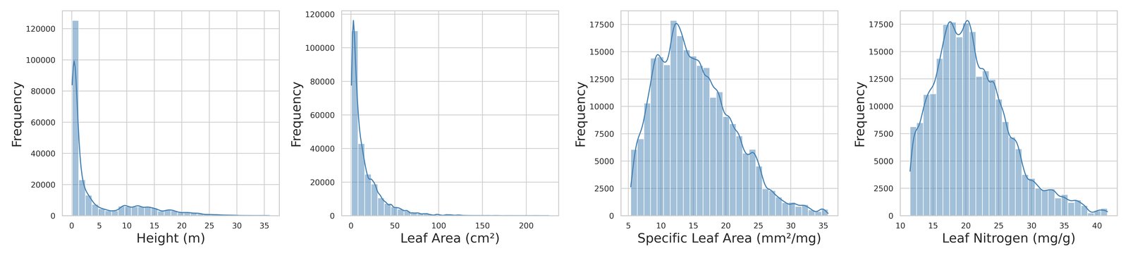
Figure 7: Distribution of median trait values at the species level in the weakly labeled citizen science training data.
图 7:弱标注公民科学训练数据中物种级性状中位数的分布。
Reference Data to Aid Uncertainty-Guided Data Cleaning
Our uncertainty-guided data cleaning strategy is grounded in the concept of a turning point—a stage during training when the model transitions from learning generalizable patterns to overfitting noisy labels (Lu and He 2022). Detecting this turning point is critical for effective uncertainty-aware data cleaning. However, in weakly supervised settings, where ground truth labels are absent or imprecise, identifying this transition reliably is challenging. To overcome this limitation, we curated a high-quality reference dataset consisting of plant images paired with accurate trait measurements. This dataset consists of smaller datasets distributed globally from various previous studies and a range of collaborators. Each collaborator contributed plant trait measurements and associated images from ecologically diverse locations, including Germany, La Palma, India, Australia, Panama, Canada, Indonesia, Switzerland, Portugal, and Namibia (see Figure 8). Detailed statistics on sample sizes and taxonomic diversity, quantified as the number of unique species, are reported in Table 3. Because different collaborators focused on specific traits, we maintain separate datasets per trait.
用于辅助不确定性引导数据清洗的参考数据
我们不确定性引导的数据清洗策略建立在转折点这一概念上:训练过程中模型从学习可泛化模式转向对嘈杂标签过拟合的阶段(Lu and He 2022)。检测这一转折点对有效的不确定性感知数据清洗至关重要。不过,在弱监督设定中,真值标签缺失或不精确,可靠识别这一转变很困难。为克服这一限制,我们整理了一个高质量参考数据集,由植物图像与准确的性状测量配对组成。该数据集由分布在全球的较小数据集构成,来自多项先前研究和一系列合作者。每位合作者贡献了来自生态多样地点的植物性状测量及相关图像,包括德国、拉帕尔马、印度、澳大利亚、巴拿马、加拿大、印度尼西亚、瑞士、葡萄牙和纳米比亚(见图 8)。关于样本量和分类多样性(以独特物种数量化)的详细统计见表 3。由于不同合作者关注特定性状,我们按性状分别维护数据集。
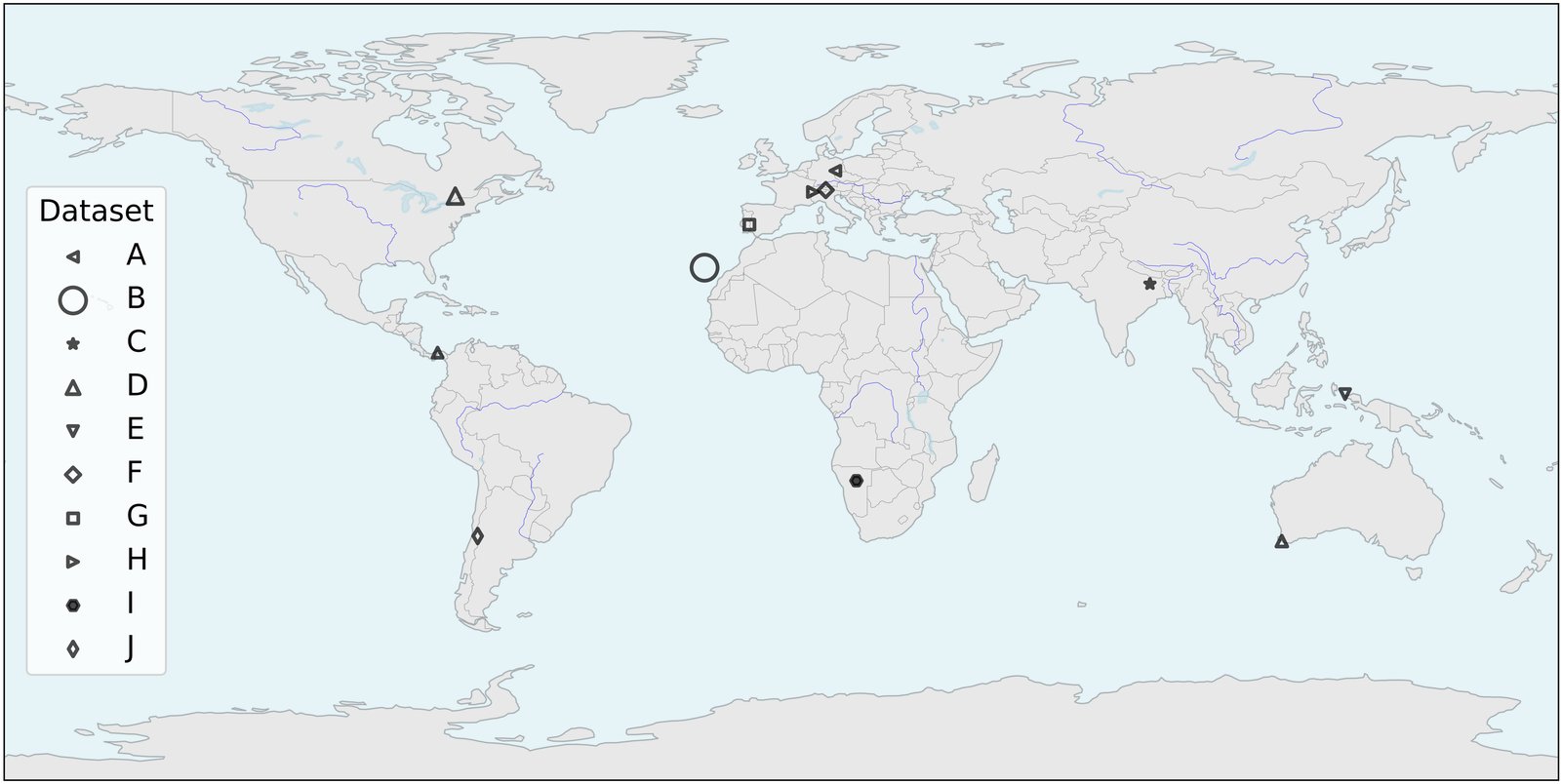
Figure 8: Locations of scientifically curated reference datasets. Marker symbols indicate distinct test data sources from Germany (A), La Palma (B), India (C), Australia (D), Panama (D), Canada (D), Indonesia (E), Switzerland (F), Portugal (G), Switzerland (H), Namibia (I), and Chile (J). Marker sizes are proportional to the corresponding dataset size.
图 8:经过科学整理的参考数据集位置。标记符号表示不同的测试数据来源:德国(A)、拉帕尔马(B)、印度(C)、澳大利亚(D)、巴拿马(D)、加拿大(D)、印度尼西亚(E)、瑞士(F)、葡萄牙(G)、瑞士(H)、纳米比亚(I)和智利(J)。标记大小与相应数据集规模成正比。
| Trait | Units | #Data points | #Species |
|---|---|---|---|
| Plant height (H) | m | 4478 | 452 |
| Leaf Area (LA) | cm2 | 2386 | 136 |
| Specific Leaf Area (SLA) | mm2/mg | 1796 | 199 |
| Leaf Nitrogen Content (LN) | mg/g | 773 | 73 |
Table 3: Metadata of the curated plant reference dataset to aid uncertainty-guided data cleaning.
| 性状 | 单位 | 数据点数 | 物种数 |
|---|---|---|---|
| 株高(H) | m | 4478 | 452 |
| 叶面积(LA) | cm2 | 2386 | 136 |
| 比叶面积(SLA) | mm2/mg | 1796 | 199 |
| 叶氮含量(LN) | mg/g | 773 | 73 |
表 3:用于辅助不确定性引导数据清洗的整理植物参考数据集元数据。
Methodology
方法
Uncertainty Estimation
To capture predictive uncertainty across traits, we model the output distribution for each trait type, denoted as . Due to its long-tailed nature, Leaf Area (LA) is modeled using a Laplace distribution, parameterized by a predicted mean and scale , where is the predicted log-scale.
不确定性估计
为了捕捉各性状的预测不确定性,我们为每种性状类型建模输出分布,记为 。由于其长尾特性,叶面积(LA)用拉普拉斯分布建模,参数为预测均值 和尺度 ,其中 是预测的对数尺度。
For Height (H), Specific Leaf Area (SLA), and Leaf Nitrogen (LN), we assume a Gaussian distribution with predicted mean and variance , where is the predicted log-variance. The negative log-likelihood (NLL) is used as the training objective: for LA, the Laplace NLL is
对株高(H)、比叶面积(SLA)和叶氮(LN),我们假定高斯分布,预测均值为 ,方差为 ,其中 是预测的对数方差。负对数似然(NLL)被用作训练目标:对 LA,拉普拉斯 NLL 为
and for the remaining traits, the Gaussian NLL is
对其余性状,高斯 NLL 为
This formulation enables the model to learn both the central tendency and the predictive uncertainty for each trait. We visualize predicted log-variance across traits in Fig. 11
这一写法使模型能够学习每个性状的中心趋势和预测不确定性。我们在图 11 中可视化各性状的预测对数方差。
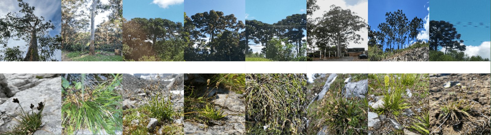
Figure 9: Visualizations of predictive uncertainty for plant height during residual-aware filtering. Example images with high uncertainty (top) and low uncertainty (bottom) are shown.
图 9:残差感知过滤期间株高预测不确定性的可视化。图中展示高不确定性(上)和低不确定性(下)的示例图像。
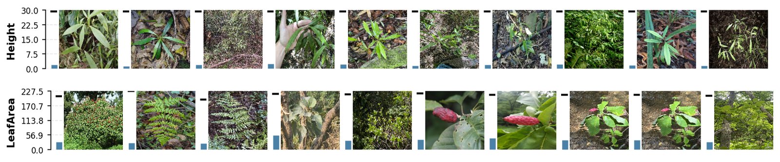
Figure 10: Examples of images with high uncertainty and high residual error identified during residual-aware filtering for Height (m) (top) and Leaf Area (cm2) (bottom). Predicted trait values are shown as bars, with species median values indicated by black dashed lines. For Height, juvenile or undeveloped individuals exhibit low predicted height but high residual error due to elevated species-level medians, leading to their removal. For Leaf Area, high residuals are associated with exotic ferns, images not focused on leaves, and small leaves from species with large median leaf areas.
图 10:在残差感知过滤中识别出的高不确定性和高残差误差图像示例,分别对应株高(米)(上)和叶面积(平方厘米)(下)。预测性状值以条形显示,物种中位数值用黑色虚线标出。对株高而言,幼株或未发育个体的预测株高较低,但由于物种级中位数偏高而产生较大残差,因而被移除。对叶面积而言,高残差与少见蕨类、未聚焦叶子的图像,以及来自中位叶面积较大物种的小叶子相关。
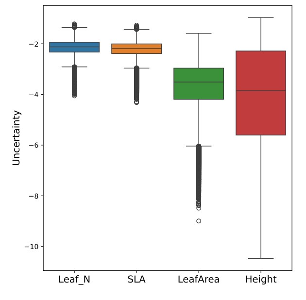
Figure 11: Visualization of the predicted log-variance values across all traits during the uncertainty-aware filtering process. Here, Leaf_N denotes leaf nitrogen, and SLA refers to specific leaf area.
图 11:不确定性感知过滤过程中所有性状预测对数方差值的可视化。这里 Leaf_N 表示叶氮,SLA 指比叶面积。
Uncertainty-Guided Data Cleaning Loop
不确定性引导的数据清洗循环
To enable scalable data curation in the presence of label noise, we propose a two-step data cleaning strategy guided by model-predicted uncertainty and residual error.
为了在存在标签噪声时实现可扩展的数据整理,我们提出一种由模型预测不确定性和残差误差引导的两步数据清洗策略。
Stage 1: Uncertainty-Aware Filtering
We employ an iterative, uncertainty-aware filtering strategy to clean the training data while a model is being trained.
阶段 1:不确定性感知过滤
我们采用迭代的、不确定性感知的过滤策略,在模型训练过程中清洗训练数据。
The model is first trained for one epoch on the full dataset. After this initial pass, we perform inference on the training set and compute predictive uncertainty across all four trait heads for each image. We then remove samples where the joint uncertainty falls within the top 5%, as we hypothesize these are likely to be visually ambiguous or noisy. Examples of such samples include poorly lit or occluded images, or those containing non-foliage content like twigs or fruit.
模型首先在完整数据集上训练一个 epoch。在这一初始遍历之后,我们在训练集上做推断,并计算每张图像在全部四个性状头上的预测不确定性。随后我们去掉联合不确定性落在最高 5% 的样本,因为我们假设这些样本很可能在视觉上含糊或嘈杂。这类样本的例子包括光照差或被遮挡的图像,或包含细枝或果实等非叶片内容的图像。
The model’s training then continues from its current state on this filtered dataset. This filtering–retraining cycle is repeated for up to two iterations or until the number of high-uncertainty samples drops below a predefined threshold.
模型随后从当前状态出发,在这一过滤后的数据集上继续训练。这一过滤–再训练循环最多重复两次,或直到高不确定性样本数降到预设阈值以下。
Step 2: Residual-Aware Filtering
As visualized in Figure 9, we observe that predictive uncertainty for traits like height increases for taller individuals, a phenomenon we hypothesize is due to heteroscedasticity. This is consistent with our observation that residuals for taller plants are generally larger than for smaller plants, leading the model to output a correspondingly higher uncertainty for taller plants. Consequently, a naive filtering approach that relies solely on high predictive uncertainty could disproportionately remove samples from larger growth forms (e.g. trees) and fail to distinguish genuinely mislabeled data from correctly labeled but uncertain predictions.
步骤 2:残差感知过滤
如图 9 所示,我们观察到株高等性状的预测不确定性会随更高的个体而增加,我们假设这是由于异方差性。这与我们的观察一致:较高植株的残差通常大于较小植株,从而使模型为较高植株输出相应更高的不确定性。因此,只依赖高预测不确定性的朴素过滤,可能不成比例地去掉来自较大生长型(例如乔木)的样本,并且无法把真正标错的数据与标签正确但不确定的预测区分开来。
To address this, we introduce residual-aware filtering. For each trait, we identify a ‘turning point’, the training epoch after which performance on an external scientific reference set begins to decline, suggesting the onset of memorization. At this checkpoint, we compute normalized mean absolute error (nMAE) between predicted trait values and species-level medians. We hypothesize that samples exhibiting both high uncertainty (above the 95th percentile) and large residual error (above 50%) are likely mislabeled or unreliable. These samples are removed over four iterations, each followed by training from scratch.
为解决这一点,我们引入残差感知过滤。对每个性状,我们识别一个“转折点”,也就是外部科学参考集上的表现开始下降之后的那个训练 epoch,这提示开始出现记忆。在这一检查点,我们计算预测性状值与物种级中位数之间的归一化平均绝对误差(nMAE)。我们假设同时表现出高不确定性(高于第 95 百分位)和大残差误差(高于 50%)的样本很可能被标错或不可靠。这些样本会在四轮迭代中被去掉,每轮之后都从头开始训练。
We visualize examples of such filtered samples for height and leaf area in Figure 10. For height, we often observe juvenile or undeveloped individuals with low predicted values but large residuals due to high species-level medians. For leaf area, examples for uncertainty samples are exotic ferns or unsharp photographs.
我们在图 10 中可视化这类被过滤样本在株高和叶面积上的例子。对株高,我们常常观察到幼株或未发育个体:预测值较低,但由于物种级中位数偏高而产生较大残差。对叶面积,不确定性样本的例子是少见蕨类或不清晰的照片。
We continue the process until the number of samples with high-residual and high-uncertainty becomes negligible. In total, we remove approximately 500 species from an initial pool of 5,500. The resulting trait distributions are shown in Figure 7. While some borderline cases may be excluded, we argue that the volume of citizen science data compensates for a reduction of the total sample size and number of species. Furthermore, given the difficulty of verifying trait labels, particularly for biochemical traits such as specific leaf area (SLA) or leaf nitrogen, we prefer cautious removal over attempting label correction.
我们持续这一过程,直到同时具有高残差和高不确定性的样本数变得可以忽略。总计我们从最初的 5500 个物种中去掉了大约 500 个物种。得到的性状分布见图 7。虽然一些边界情形可能被排除,我们认为公民科学数据的体量可以补偿总样本量和物种数的减少。此外,鉴于核实性状标签很困难,对 SLA 或叶氮等生化性状尤其如此,我们更倾向于谨慎移除,而不是尝试校正标签。
Experiment
实验
Experimental Setup
Data Preprocessing. In both the global plant kingdom and citizen science datasets, grassland species are the most frequently observed growth form, followed by shrubs, with tree species being the least represented. Blindly training on such imbalanced data would likely bias the model toward frequent grassland species, reducing its ability to generalize to less common growth forms. To mitigate this, we stratified the data by growth forms and applied weighted sampling during training. Each batch was constructed to contain a balanced mix of grasses, shrubs, and trees, ensuring more equitable learning across growth forms. Lastly, all continuous target traits were normalized to the range [0, 1] using MinMax scaling.
实验设置
数据预处理。 在全球植物界和公民科学数据集中,草地物种都是最常被观测到的生长型,其次是灌木,乔木物种代表性最少。如果在这种不平衡数据上盲目训练,模型很可能偏向常见的草地物种,从而降低对较不常见生长型的泛化能力。为减轻这一点,我们按生长型对数据分层,并在训练时施加加权抽样。每个批次被构造成包含草本、灌木和乔木的均衡组合,以确保跨生长型更公平地学习。最后,所有连续目标性状都用 MinMax 缩放归一化到 [0, 1] 范围。
Training Procedure. The model is trained for 30 epochs using the AdamW optimizer with , and a weight decay of . A cosine annealing learning rate schedule decays the learning rate from an initial value of to a minimum of . Training stability is further ensured by gradient clipping with a maximum norm of 1.0.
训练过程。 模型使用 AdamW 优化器训练 30 个 epoch,,权重衰减为 。余弦退火学习率日程把学习率从初值 衰减到最小值 。梯度裁剪的最大范数为 1.0,以进一步保证训练稳定。
Results
结果
Global Maps Trait Maps derived from Aggregated PlantTraitNet Predictions
Figure 12 show global maps at 1 degree resolution obtained from aggregating predicted traits from PlantTraitNet on 300k citizen science images. In addition to the quantitative evaluation against vegetation surveys (sPlotOpen, next section), we found that the global patterns reproduce expected global trait patterns (Lusk et al. 2025; Wolf et al. 2022). For instance, for height and leaf area, we find expected longitudinal variation, such as large plants with big leaves towards the equator. Most robust plants (high specific leaf area and nitrogen content) are found in temperate and boreal zones.
由聚合 PlantTraitNet 预测得到的全球性状图
图 12 展示了在 30 万张公民科学图像上聚合 PlantTraitNet 预测性状后、以 1 度分辨率得到的全球图。除了下一节相对植被调查(sPlotOpen)的定量评估外,我们发现全球格局能够再现预期的全球性状模式(Lusk et al. 2025; Wolf et al. 2022)。例如,对株高和叶面积,我们看到预期的经向变化,例如靠近赤道出现更大的植物和更大的叶子。最强壮的植物(高比叶面积和氮含量)出现在温带和寒带。
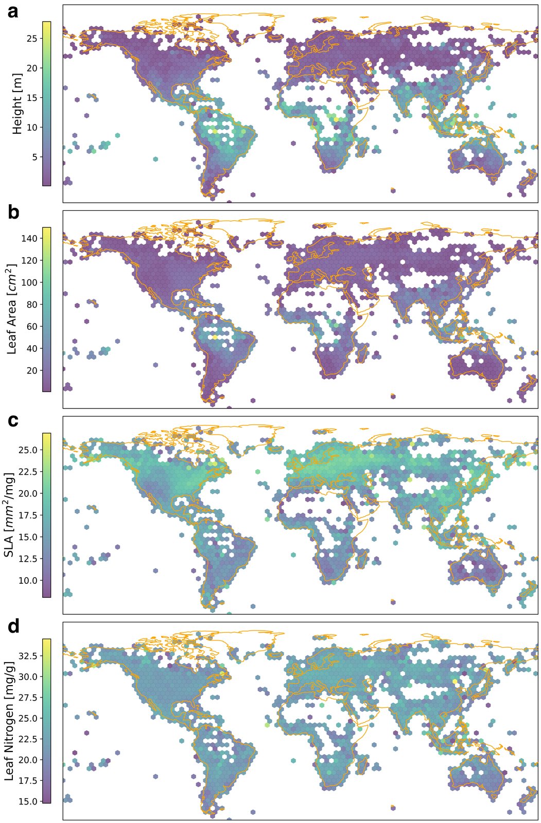
Figure 12: Global trait maps derived from spatially aggregating PlantTraitNet predictions at 1 degree resolution. The global trait maps comprise height (a), SLA (b), leaf area (c), and leaf nitrogen (d) based on the spatial aggregation of citizen science photos from the validation dataset.
图 12:把 PlantTraitNet 预测在空间上聚合到 1 度分辨率后得到的全球性状图。全球性状图包括株高(a)、SLA(b)、叶面积(c)和叶氮(d),基于验证数据集中公民科学照片的空间聚合。
Evaluating Global Trait Maps from PlantTraitNet with Vegetation Survey data (sPlotOpen)
To empirically demonstrate the effectiveness of our uncertainty-guided data cleaning process, we compare model performance on raw (unfiltered) and refined dataset (Table 4). Performance is evaluated using , nMAE, and Pearson’s , with results averaged over three independent runs.
用植被调查数据(sPlotOpen)评估来自 PlantTraitNet 的全球性状图
为了经验地展示不确定性引导数据清洗过程的有效性,我们比较模型在原始(未过滤)和清洗后数据集上的表现(表 4)。评估使用 、nMAE 和皮尔逊 ,结果在三次独立运行上取平均。
We observe that our data refinement process leads to consistent improvements in predictive performance. Notably, for SLA and LA increases from 0.23 to 0.27 and 0.30 to 0.34, respectively, demonstrating enhanced predictive reliability. For Leaf Nitrogen (LN), although the model’s overall performance is limited (negative ), the refined dataset still yields a marginal improvement in correlation ( vs. 0.49).
我们观察到,数据 refinement 过程会带来预测表现的持续改进。值得注意的是,SLA 和 LA 的 分别从 0.23 提高到 0.27、从 0.30 提高到 0.34,说明预测可靠性有所增强。对叶氮(LN),尽管模型的总体表现有限( 为负),清洗后的数据集仍在相关性上带来轻微改进( 对 0.49)。
The results, visualized in Figure 13, indicate that filtering noisy samples is a key step toward more robust and reliable trait predictions from our citizen science data.
如图 13 所示的结果表明,过滤嘈杂样本是从我们的公民科学数据中获得更稳健、更可靠性状预测的关键一步。
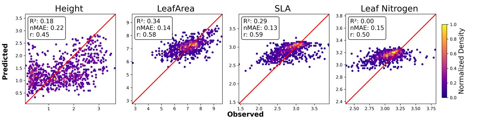
Figure 13: Global trait predictions obtained from PlantTraitNet against globally distributed vegetation survey data (sPlotOpen). Trait predictions of geotagged images are aggregated at a 1° spatial resolution using image geolocations (Predicted). These aggregated predictions are then compared with averaged community-weighted trait values derived from sPlotOpen (Observed).
图 13:PlantTraitNet 得到的全球性状预测与全球分布的植被调查数据(sPlotOpen)对照。带地理标签图像的性状预测按图像地理位置聚合到 1° 空间分辨率(预测)。这些聚合预测随后与来自 sPlotOpen 的平均群落加权性状值(观测)比较。
| Method | Metric | H | LA | SLA | LN |
|---|---|---|---|---|---|
| Ours (Raw) | ↑ | 0.19 ± 0.01 | 0.30 ± 0.04 | 0.23 ± 0.01 | -0.16 ± 0.03 |
| nMAE ↓ | 0.22 ± 0.00 | 0.14 ± 0.00 | 0.14 ± 0.00 | 0.17 ± 0.00 | |
| ↑ | 0.45 ± 0.01 | 0.56 ± 0.01 | 0.59 ± 0.01 | 0.49 ± 0.01 | |
| Ours (Refined) | ↑ | 0.18 ± 0.00 | 0.34 ± 0.01 | 0.27 ± 0.02 | -0.12 ± 0.14 |
| nMAE ↓ | 0.22 ± 0.0 | 0.14 ± 0.0 | 0.13 ± 0.00 | 0.17 ± 0.01 | |
| ↑ | 0.45 ± 0.00 | 0.57 ± 0.00 | 0.59 ± 0.01 | 0.50 ± 0.00 |
Table 4: Comparison of PlantTraitNet with sPlotOpen community weighted trait means at 1° resolution. We report mean standard deviation across 3 runs with different random initializations. Raw refers to models trained with unfiltered citizen science data, while refined refers models based on the uncertainty-aware training.
| 方法 | 指标 | H | LA | SLA | LN |
|---|---|---|---|---|---|
| 本文(原始) | ↑ | 0.19 ± 0.01 | 0.30 ± 0.04 | 0.23 ± 0.01 | -0.16 ± 0.03 |
| nMAE ↓ | 0.22 ± 0.00 | 0.14 ± 0.00 | 0.14 ± 0.00 | 0.17 ± 0.00 | |
| ↑ | 0.45 ± 0.01 | 0.56 ± 0.01 | 0.59 ± 0.01 | 0.49 ± 0.01 | |
| 本文(清洗后) | ↑ | 0.18 ± 0.00 | 0.34 ± 0.01 | 0.27 ± 0.02 | -0.12 ± 0.14 |
| nMAE ↓ | 0.22 ± 0.0 | 0.14 ± 0.0 | 0.13 ± 0.00 | 0.17 ± 0.01 | |
| ↑ | 0.45 ± 0.00 | 0.57 ± 0.00 | 0.59 ± 0.01 | 0.50 ± 0.00 |
表 4:PlantTraitNet 与 sPlotOpen 群落加权性状均值在 1° 分辨率上的比较。我们报告三次不同随机初始化运行的均值 标准差。原始指在未过滤公民科学数据上训练的模型,清洗后指基于不确定性感知训练的模型。
Qualitative Assessment of Intraspecific Trait Variability
Trait values within a species can vary across environmental gradients and hence an accurate representation of intraspecific variability can be important to create global trait maps. However, the weak annotations used for model training were based on species-level matching of citizen science photographs and trait values from the TRY database. Accordingly, the model was not explicitly trained to capture within-species variability. To qualitatively evaluate if PlantTraitNet still captures intraspecific trait variation, we analyzed model predictions for ecologically diverse species across major growth forms, including grasses, shrubs, and trees. For each selected species, we conducted two complementary analyses:
种内性状变异性的定性评估
同一物种内的性状值可以沿环境梯度变化,因此准确表示种内变异性对创建全球性状图可能很重要。不过,用于模型训练的弱标注基于公民科学照片与 TRY 数据库性状值的物种级匹配。因此,模型并没有被显式训练去捕捉种内变异性。为了定性评估 PlantTraitNet 是否仍然捕捉种内性状变异,我们分析了覆盖主要生长型(包括草本、灌木和乔木)的生态多样物种的模型预测。对每个选定物种,我们进行了两项互补分析:
- We visualized predicted trait values for a small, held-out subset of seven individuals that exhibited notable visual variation in developmental stage, size or structure.
- 我们可视化了一个小型、留出的七个个体子集的预测性状值,这些个体在发育阶段、大小或结构上表现出显著的视觉差异。
- We compared the distribution of predicted trait values from up to 100 training images to the corresponding distribution of observed trait values from up to 100 samples in the TRY database.
- 我们把最多 100 张训练图像的预测性状值分布,与 TRY 数据库中最多 100 个样本的相应观测性状值分布进行比较。
This analysis provides insight into how well the model reflects trait variability within species, relative to aggregated trait observations. Our results, visualized in Figures 15, 16, 17 and 18, consistently show that the model learns to represent a wide range of intraspecific variation for traits like Height (H) and Leaf Area (LA). In these cases, the predicted trait ranges often exceeded the variation captured in the original TRY database observations. This seems plausible, given that trait observations are typically performed on healthy and adult plants. Compared to Leaf Area (LA) and Plant Height (H), for physiological traits such as Specific Leaf Area (SLA) and Leaf Nitrogen (LN), we observe little predicted variation. We hypothesize this is a positive outcome, as these leaf traits are ecologically expected to show less intraspecific variability on the premise that interspecific trait variation generally exceeds intraspecific variation (Dong et al. 2020; Wright et al. 2017). For improved visibility, only predicted values between the 5th and 95th percentiles are shown.
这一分析有助于理解模型在物种内部反映性状变异性的程度,相对于聚合的性状观测而言。如图 15、16、17 和 18 所示,我们的结果一致表明,模型学会了表示株高(H)和叶面积(LA)一类性状的广泛种内变异。在这些情形中,预测性状范围常常超过原始 TRY 数据库观测所捕捉到的变异。这看起来是合理的,因为性状观测通常在健康的成年植株上进行。与叶面积(LA)和株高(H)相比,对比叶面积(SLA)和叶氮(LN)等生理性状,我们观察到的预测变异较少。我们假设这是一个正面结果,因为这些叶片性状在生态上预期会显示较少的种内变异性,其前提是种间性状变异通常超过种内变异(Dong et al. 2020; Wright et al. 2017)。为提高可见性,图中只显示第 5 到第 95 百分位之间的预测值。
| Trait Error | K | K* | Lambda |
|---|---|---|---|
| H | 0.018 | 0.015 | 0.801 |
| (p = 0.001) | (p = 0.001) | (p = 0.001) | |
| LA | 0.007 | 0.007 | 0.556 |
| (p = 0.064) | (p = 0.079) | (p = 0.001) | |
| SLA | 0.005 | 0.006 | 0.042 |
| (p = 0.441) | (p = 0.399) | (p = 0.003) | |
| LN | 0.008 | 0.008 | 0.150 |
| (p = 0.001) | (p = 0.001) | (p = 0.001) |
Table 5: Phylogenetic signal metrics with corresponding p-values
| 性状误差 | K | K* | Lambda |
|---|---|---|---|
| H | 0.018 | 0.015 | 0.801 |
| (p = 0.001) | (p = 0.001) | (p = 0.001) | |
| LA | 0.007 | 0.007 | 0.556 |
| (p = 0.064) | (p = 0.079) | (p = 0.001) | |
| SLA | 0.005 | 0.006 | 0.042 |
| (p = 0.441) | (p = 0.399) | (p = 0.003) | |
| LN | 0.008 | 0.008 | 0.150 |
| (p = 0.001) | (p = 0.001) | (p = 0.001) |
表 5:系统发育信号指标及相应 p 值
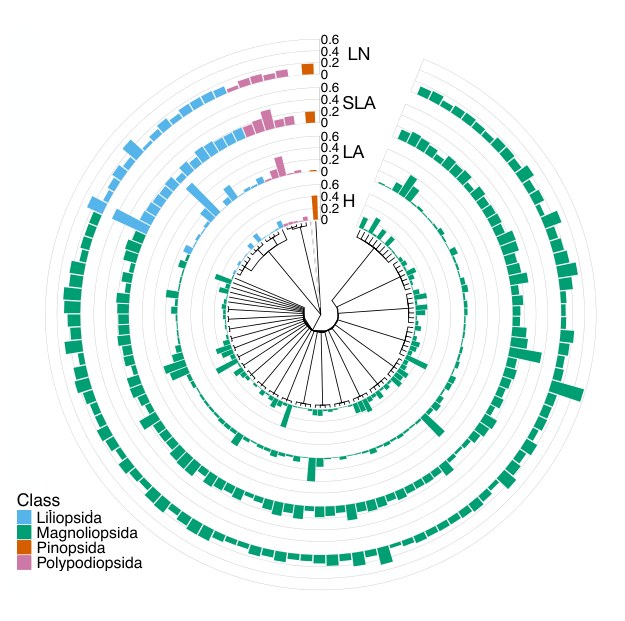
Trait Prediction Error Along the Taxonomic Tree
Figure 14: Mean relative prediction error (MRPE) computed on validation data at the family level, visualized along the taxonomic tree, for height (H), leaf area (LA), specific leaf area (SLA) and leaf nitrogen (LN).
沿分类树的性状预测误差
图 14:在验证数据上按科计算的平均相对预测误差(MRPE),沿分类树可视化,分别对应株高(H)、叶面积(LA)、比叶面积(SLA)和叶氮(LN)。
A phylogenetic tree was constructed from hierarchical taxonomic information (Kingdom to Species) using as.phylo() from the ape package (Paradis and Schliep 2019). Mean relative errors (MRE) were computed per species, normalized by the trait-specific error range, and matched with taxonomic metadata. In Figure 14, MREs are shown at the family and class levels, with no clear visual pattern of systematic bias. Moreover, we report standard metrics to quantify the phylogenetic signal in species-level prediction errors, calculated via the phyloSignal() function from the phylosignal R package. Pagel’s (Pagel 1999) measures the overall fit of the data to the phylogeny by scaling internal branches; values close to 1 indicate a strong phylogenetic structure, while values near 0 suggest independence from phylogeny. Statistical significance is assessed by comparing the fitted to a model with . Blomberg’s (Blomberg et al. 2003) compares the observed trait variance across the tree to expectations under a Brownian motion model; values close to 1 indicate strong signal, and values 1 suggest weak signal, especially among closely related species. is a variation of that is less sensitive to tree imbalance and branch length distortions. Together, these metrics offer complementary perspectives on phylogenetic structure at different evolutionary scales (see Table 5). Pagel’s captures broad-scale phylogenetic autocorrelation in residual covariance (Pagel 1999), while Blomberg’s is more sensitive to fine-scale signal among closely related species (Blomberg et al. 2003). For SLA and leaf nitrogen, the phylogenetic signal is weak ( = 0.04 and 0.15; = 0.0053 and 0.0076), suggesting that prediction errors are largely independent of species relatedness. Although errors for height ( = 0.80, = 0.018) and leaf area ( = 0.56, = 0.0067) show some phylogenetic autocorrelation, the consistently low values indicate that even closely related species do not share systematic prediction biases. These results reveal that while slight patterns may emerge at the level of broader plant classes, there is no consistent phylogenetic structure among closely related species. Altogether, this underscores that despite being trained on species-level annotations, the model exhibits strong generalizability and methodological robustness for predicting plant traits across the plant kingdom.
系统发育树由从界到种的层次分类信息,用 ape 软件包中的 as.phylo() 构建(Paradis and Schliep 2019)。平均相对误差(MRE)按物种计算,用性状特定的误差范围归一化,并与分类元数据匹配。在图 14 中,MRE 显示在科和纲的层级上,没有清晰可见的系统偏差模式。此外,我们报告用于量化物种级预测误差中系统发育信号的标准指标,这些指标通过 phylosignal R 软件包中的 phyloSignal() 函数计算。Pagel 的 (Pagel 1999)通过缩放内部枝长来衡量数据对系统发育的总体拟合;接近 1 的值表示强的系统发育结构,接近 0 的值则提示独立于系统发育。统计显著性通过把拟合的 与 的模型比较来评估。Blomberg 的 (Blomberg et al. 2003)把树上观测到的性状方差与布朗运动模型下的期望进行比较;接近 1 的值表示强信号,远小于 1 的值则提示信号弱,在近缘种之间尤其如此。 是 的一个变体,对树的不平衡和枝长扭曲不那么敏感。这些指标一起,为不同进化尺度上的系统发育结构提供了互补视角(见表 5)。Pagel 的 捕捉残差协方差中的大尺度系统发育自相关(Pagel 1999),而 Blomberg 的 对近缘种之间的细尺度信号更敏感(Blomberg et al. 2003)。对 SLA 和叶氮,系统发育信号较弱( = 0.04 和 0.15; = 0.0053 和 0.0076),说明预测误差大体上独立于物种亲缘关系。尽管株高( = 0.80, = 0.018)和叶面积( = 0.56, = 0.0067)的误差显示出一些系统发育自相关,一贯偏低的 值表明,即便近缘种也不共享系统的预测偏差。这些结果表明,虽然在更宽的植物纲层级上可能出现轻微模式,近缘种之间并没有一致的系统发育结构。总的来说,这强调了尽管模型在物种级标注上训练,它在预测整个植物界的植物性状时仍表现出很强的泛化能力和方法稳健性。
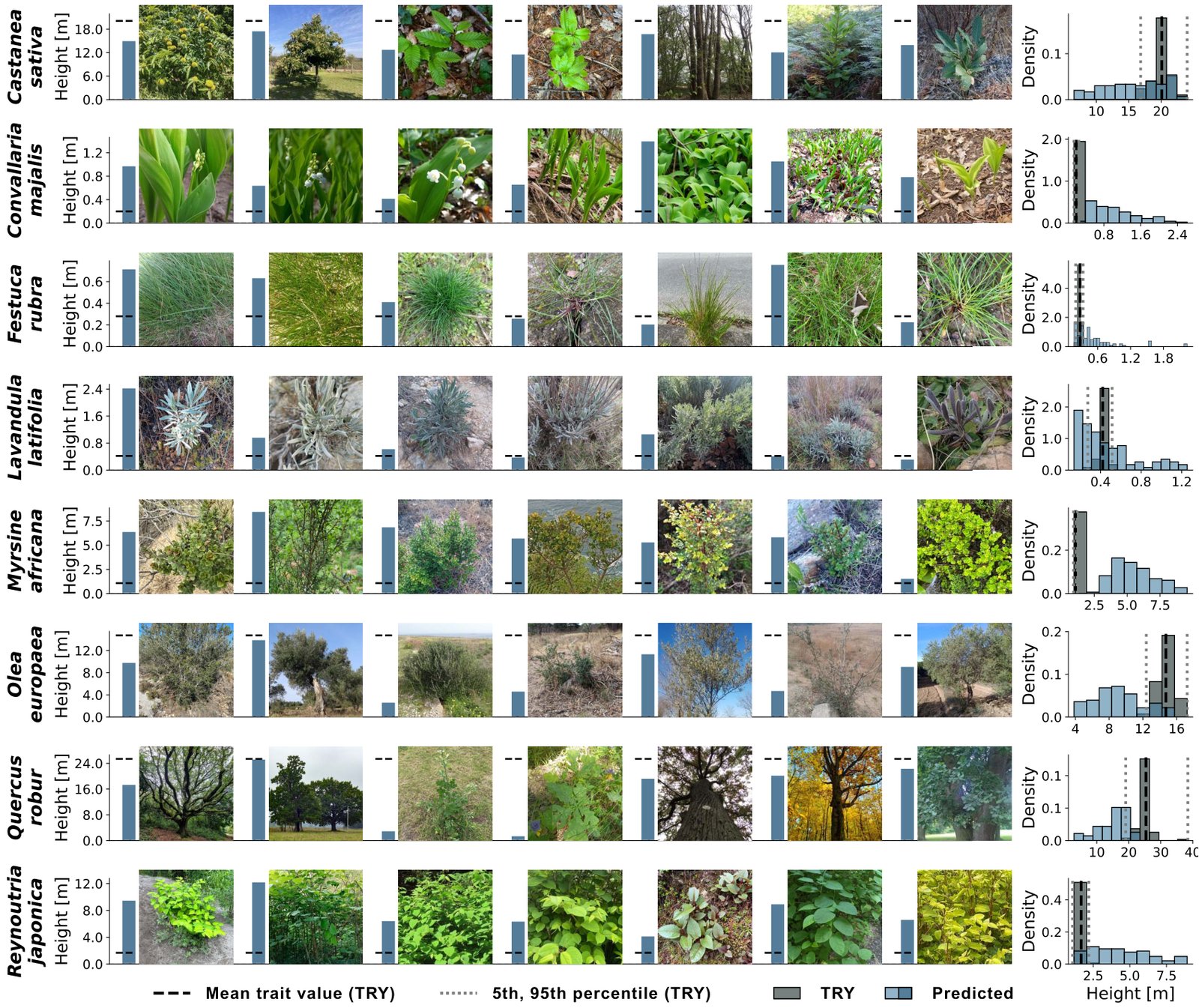
Figure 15: Intraspecific variation in predicted plant height compared to TRY-derived trait means.
图 15:预测株高中的种内变异,与来自 TRY 的性状均值比较。
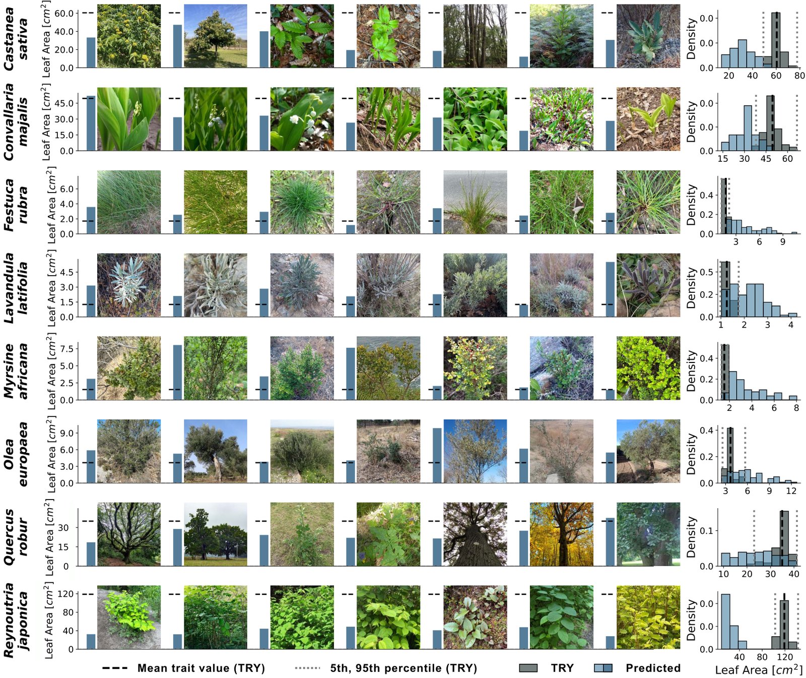
Figure 16: Intraspecific variation in predicted leaf area compared to TRY-derived trait means.
图 16:预测叶面积中的种内变异,与来自 TRY 的性状均值比较。
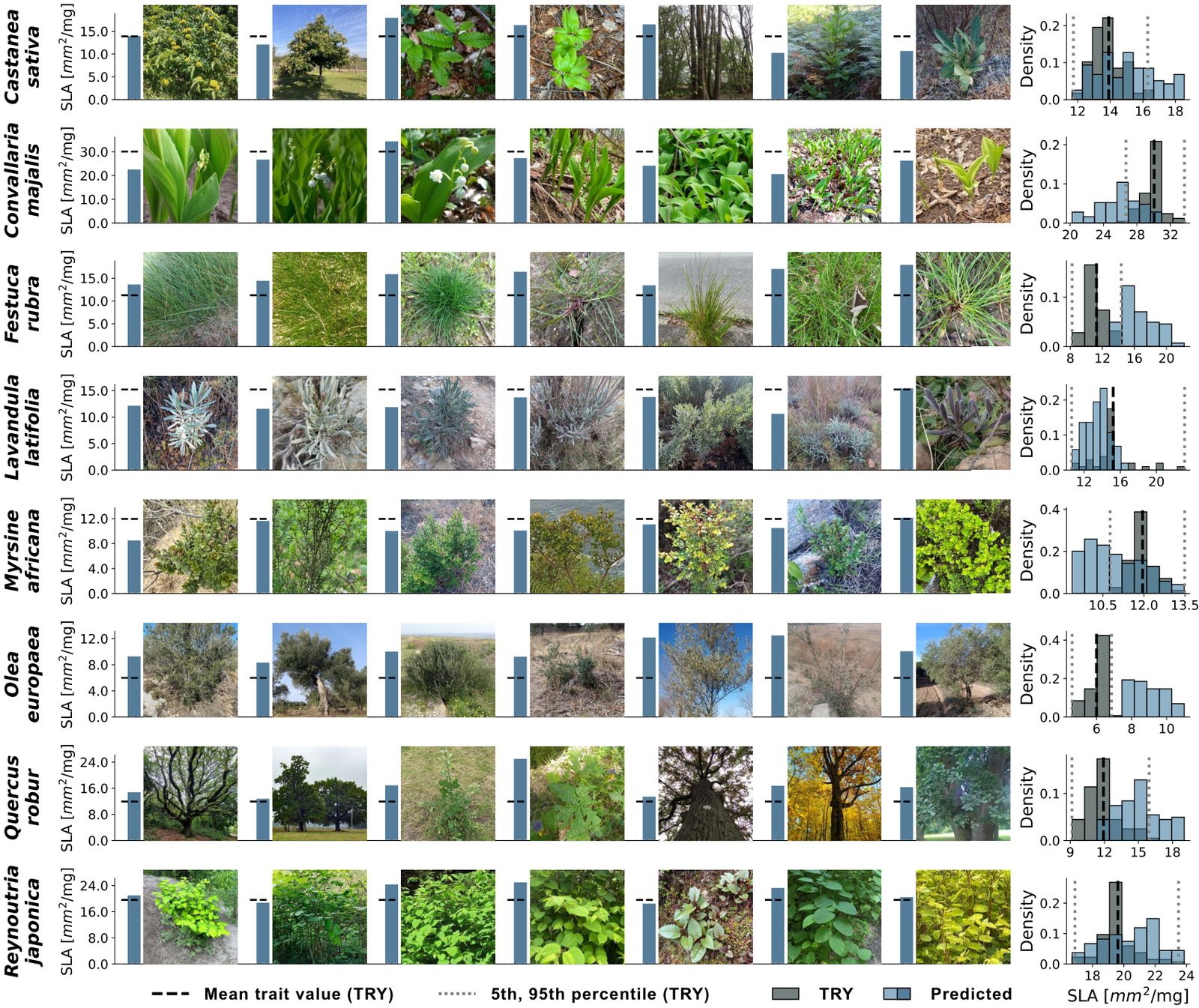
Figure 17: Intraspecific variation in predicted specific leaf area compared to TRY-derived trait means.
图 17:预测比叶面积中的种内变异,与来自 TRY 的性状均值比较。
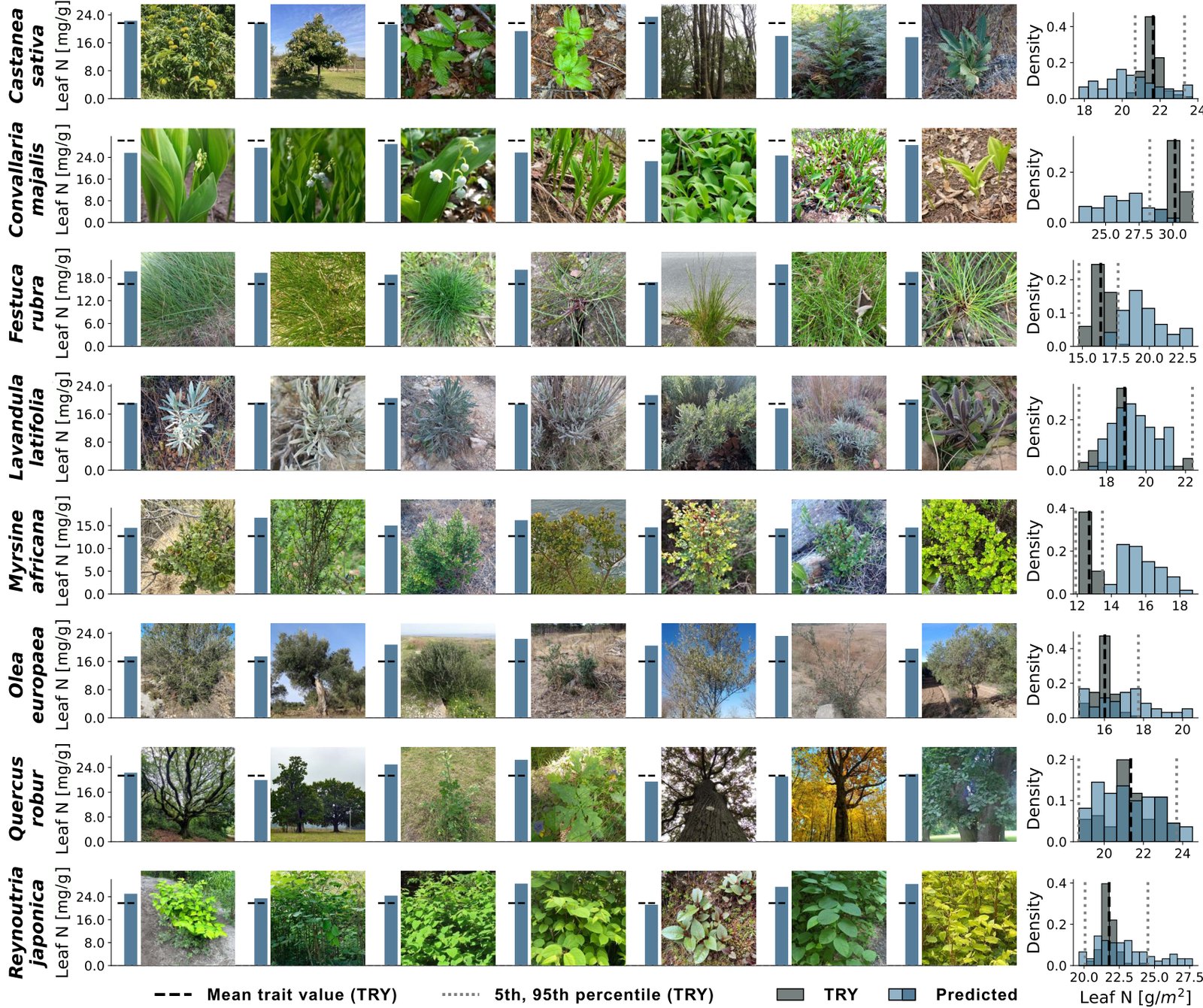
Figure 18: Intraspecific variation in predicted leaf nitrogen compared to TRY-derived trait means.
图 18:预测叶氮中的种内变异,与来自 TRY 的性状均值比较。
| Method | H | LA | SLA | LN |
|---|---|---|---|---|
| Gaussian | 0.18 ± 0.02 | 0.31 ± 0.01 | 0.31 ± 0.01 | 0.18 ± 0.01 |
| Laplace (LA + H) | 0.10 ± 0.01 | 0.32 ± 0.01 | 0.32 ± 0.02 | 0.18 ± 0.03 |
| Laplace (LA) | 0.19 ± 0.02 | 0.32 ± 0.01 | 0.31 ± 0.02 | 0.18 ± 0.05 |
Table 6: Impact of trait-specific loss functions on predictive performance. Reported values are mean ± one standard deviation across three independently initialized training runs for each loss configuration.
| 方法 | H | LA | SLA | LN |
|---|---|---|---|---|
| 高斯 | 0.18 ± 0.02 | 0.31 ± 0.01 | 0.31 ± 0.01 | 0.18 ± 0.01 |
| 拉普拉斯(LA + H) | 0.10 ± 0.01 | 0.32 ± 0.01 | 0.32 ± 0.02 | 0.18 ± 0.03 |
| 拉普拉斯(LA) | 0.19 ± 0.02 | 0.32 ± 0.01 | 0.31 ± 0.02 | 0.18 ± 0.05 |
表 6:性状特定损失函数对预测表现的影响。报告值为每种损失配置下三次独立初始化训练运行的平均 ± 一个标准差。
| Image Encoder | H | LA | SLA | LN |
|---|---|---|---|---|
| DINOv2 (CLS token) | 0.18 ± 0.01 | 0.31 ± 0.00 | 0.30 ± 0.01 | 0.11 ± 0.01 |
| DINOv2 (patch mean) | 0.15 ± 0.00 | 0.31 ± 0.00 | 0.32 ± 0.00 | 0.14 ± 0.01 |
| BioCLIP (CLS token) | 0.15 ± 0.01 | 0.30 ± 0.00 | 0.32 ± 0.01 | 0.15 ± 0.04 |
| BioCLIP (patch mean) | 0.17 ± 0.01 | 0.30 ± 0.01 | 0.31 ± 0.01 | 0.12 ± 0.05 |
Table 7: Integrating embeddings from patch token vs. classification token (CLS) in image encoders. We report 1 standard deviation across 3 runs.
| 图像编码器 | H | LA | SLA | LN |
|---|---|---|---|---|
| DINOv2(CLS token) | 0.18 ± 0.01 | 0.31 ± 0.00 | 0.30 ± 0.01 | 0.11 ± 0.01 |
| DINOv2(patch 均值) | 0.15 ± 0.00 | 0.31 ± 0.00 | 0.32 ± 0.00 | 0.14 ± 0.01 |
| BioCLIP(CLS token) | 0.15 ± 0.01 | 0.30 ± 0.00 | 0.32 ± 0.01 | 0.15 ± 0.04 |
| BioCLIP(patch 均值) | 0.17 ± 0.01 | 0.30 ± 0.01 | 0.31 ± 0.01 | 0.12 ± 0.05 |
表 7:在图像编码器中整合 patch token 与分类 token(CLS)的嵌入。我们报告 3 次运行的 1 个标准差。
| Image | Geo | Multimodal | H | LA | SLA | LN |
|---|---|---|---|---|---|---|
| Backbone Dim | ||||||
| DinoV2(patch) + Climplicit | ||||||
| 512 | 256 | 768 | 0.18 ± 0.01 | 0.30 ± 0.01 | 0.30 ± 0.01 | 0.13 ± 0.04 |
| 768 | 256 | 768 | 0.19 ± 0.01 | 0.32 ± 0.01 | 0.31 ± 0.01 | 0.16 ± 0.06 |
| 768 | 256 | 1024 | 0.18 ± 0.02 | 0.30 ± 0.03 | 0.29 ± 0.01 | 0.12 ± 0.02 |
| 768 | 1024 | 768 | 0.18 ± 0.00 | 0.31 ± 0.01 | 0.29 ± 0.02 | 0.12 ± 0.03 |
| 768 | 1024 | 1024 | 0.17 ± 0.01 | 0.30 ± 0.03 | 0.28 ± 0.01 | 0.13 ± 0.03 |
| 768 | 512 | 768 | 0.18 ± 0.01 | 0.32 ± 0.02 | 0.29 ± 0.01 | 0.14 ± 0.05 |
| 768 | 512 | 1024 | 0.17 ± 0.01 | 0.31 ± 0.01 | 0.3 ± 0.01 | 0.14 ± 0.02 |
| DinoV2(patch) + SatCLIP | ||||||
| 768 | 256 | 768 | 0.16 ± 0.02 | 0.27 ± 0.04 | 0.25 ± 0.02 | 0.11 ± 0.05 |
| 768 | 256 | 1024 | 0.13 ± 0.03 | 0.26 ± 0.03 | 0.25 ± 0.01 | 0.13 ± 0.01 |
| DinoV2(patch) + GeoCLIP | ||||||
| 768 | 256 | 768 | 0.17 ± 0.01 | 0.33 ± 0.01 | 0.32 ± 0.00 | 0.15 ± 0.01 |
| 768 | 256 | 1024 | 0.16 ± 0.01 | 0.33 ± 0.00 | 0.31 ± 0.01 | 0.15 ± 0.02 |
| 768 | 512 | 768 | 0.17 ± 0.0 | 0.32 ± 0.01 | 0.32 ± 0.00 | 0.13 ± 0.02 |
| 768 | 512 | 1024 | 0.17 ± 0.0 | 0.3 ± 0.0 | 0.31 ± 0.01 | 0.13 ± 0.02 |
| DinoV2(patch) + Climplicit(256-D) + Depth(768-D) | ||||||
| 768 | 256 | 768 | 0.17 ± 0.02 | 0.32 ± 0.02 | 0.32 ± 0.01 | 0.16 ± 0.03 |
| 768 | 256 | 1024 | 0.19 ± 0.02 | 0.32 ± 0.01 | 0.31 ± 0.02 | 0.18 ± 0.05 |
Table 8: Effect of embedding size for each modality and the multimodal backbone. We perform ablations over different embedding dimensions: [512, 768] for image encoders, [256, 512, 1024] for geospatial encoders, and [768, 1024] for the multimodal fusion layer. We report 1 standard deviation across 3 runs.
| 图像 | 地理 | 多模态 | H | LA | SLA | LN |
|---|---|---|---|---|---|---|
| 主干维数 | ||||||
| DinoV2(patch) + Climplicit | ||||||
| 512 | 256 | 768 | 0.18 ± 0.01 | 0.30 ± 0.01 | 0.30 ± 0.01 | 0.13 ± 0.04 |
| 768 | 256 | 768 | 0.19 ± 0.01 | 0.32 ± 0.01 | 0.31 ± 0.01 | 0.16 ± 0.06 |
| 768 | 256 | 1024 | 0.18 ± 0.02 | 0.30 ± 0.03 | 0.29 ± 0.01 | 0.12 ± 0.02 |
| 768 | 1024 | 768 | 0.18 ± 0.00 | 0.31 ± 0.01 | 0.29 ± 0.02 | 0.12 ± 0.03 |
| 768 | 1024 | 1024 | 0.17 ± 0.01 | 0.30 ± 0.03 | 0.28 ± 0.01 | 0.13 ± 0.03 |
| 768 | 512 | 768 | 0.18 ± 0.01 | 0.32 ± 0.02 | 0.29 ± 0.01 | 0.14 ± 0.05 |
| 768 | 512 | 1024 | 0.17 ± 0.01 | 0.31 ± 0.01 | 0.3 ± 0.01 | 0.14 ± 0.02 |
| DinoV2(patch) + SatCLIP | ||||||
| 768 | 256 | 768 | 0.16 ± 0.02 | 0.27 ± 0.04 | 0.25 ± 0.02 | 0.11 ± 0.05 |
| 768 | 256 | 1024 | 0.13 ± 0.03 | 0.26 ± 0.03 | 0.25 ± 0.01 | 0.13 ± 0.01 |
| DinoV2(patch) + GeoCLIP | ||||||
| 768 | 256 | 768 | 0.17 ± 0.01 | 0.33 ± 0.01 | 0.32 ± 0.00 | 0.15 ± 0.01 |
| 768 | 256 | 1024 | 0.16 ± 0.01 | 0.33 ± 0.00 | 0.31 ± 0.01 | 0.15 ± 0.02 |
| 768 | 512 | 768 | 0.17 ± 0.0 | 0.32 ± 0.01 | 0.32 ± 0.00 | 0.13 ± 0.02 |
| 768 | 512 | 1024 | 0.17 ± 0.0 | 0.3 ± 0.0 | 0.31 ± 0.01 | 0.13 ± 0.02 |
| DinoV2(patch) + Climplicit(256-D) + Depth(768-D) | ||||||
| 768 | 256 | 768 | 0.17 ± 0.02 | 0.32 ± 0.02 | 0.32 ± 0.01 | 0.16 ± 0.03 |
| 768 | 256 | 1024 | 0.19 ± 0.02 | 0.32 ± 0.01 | 0.31 ± 0.02 | 0.18 ± 0.05 |
表 8:各模态和多模态主干嵌入大小的影响。我们在不同嵌入维度上做消融:图像编码器为 [512, 768],地理空间编码器为 [256, 512, 1024],多模态融合层为 [768, 1024]。我们报告 3 次运行的 1 个标准差。
Ablation Study
消融研究
Effect of Trait-Specific Loss Functions
性状特定损失函数的影响
Plant traits can differ strongly in their distributions, which in turn can affect the model training. To investigate the influence of loss function choice on trait prediction, we compare Gaussian and trait-specific Laplace loss formulations, as shown in Table 6. Given the long-tailed distributions observed for certain traits, notably leaf area (LA) and height (H) (see Figure 7), we hypothesize that the heavier-tailed Laplace loss may improve model robustness and calibration. Applying the Laplace loss to LA results in performance improvements compared to the Gaussian loss for both LA and height, while performance for SLA and LN remains similar. However, applying the Laplace loss to both LA and H decreases performance for height. This outcome may be related to the height distribution being heavily influenced by grass species, causing imbalance. Since we mitigate this imbalance through stratified sampling across plant functional types such as grasses, shrubs, and trees, the Gaussian loss appears more appropriate for modeling height under these conditions. In summary, our results suggest that trait-specific loss functions can benefit LA prediction. Based on this analysis, we adopt a hybrid approach in the final model, using the Laplace loss for LA and Gaussian losses for the other traits. This approach is associated with improved predictive performance across traits and underlines that model training requires careful consideration of multivariate ecological complexity.
植物性状的分布可能差异很大,这反过来会影响模型训练。为了考察损失函数选择对性状预测的影响,我们比较高斯损失和性状特定的拉普拉斯损失写法,如表 6 所示。鉴于某些性状、尤其是叶面积(LA)和株高(H)观察到的长尾分布(见图 7),我们假设尾部更重的拉普拉斯损失可能提高模型稳健性和校准。把拉普拉斯损失用于 LA,会相对高斯损失同时改进 LA 和株高的表现,而 SLA 和 LN 的表现保持类似。不过,把拉普拉斯损失同时用于 LA 和 H 会降低株高表现。这一结果可能与株高分布受到草本物种的强烈影响、从而造成不平衡有关。由于我们通过按草本、灌木和乔木等植物功能型分层抽样来减轻这种不平衡,在这些条件下高斯损失看起来更适合建模株高。总之,我们的结果表明,性状特定的损失函数可以使 LA 预测受益。基于这一分析,我们在最终模型中采用混合做法:对 LA 使用拉普拉斯损失,对其余性状使用高斯损失。这一做法与跨性状更好的预测表现相关,并强调模型训练需要审慎考虑多元生态复杂性。
Effect of Token Pooling Strategy on Trait Prediction Performance
While the classification token (‘[CLS]’) is a common choice for a global image representation, the individual patch tokens of vision transformers contain rich, spatially-aware information that can be more beneficial for downstream tasks (Caron et al. 2021). We therefore perform an ablation study to determine the optimal token representation for our trait prediction task (Table 7).
Token 池化策略对性状预测表现的影响
虽然分类 token(‘[CLS]’)是全局图像表示的常见选择,视觉 Transformer 的各个 patch token 包含丰富的、具有空间感知的信息,可能对下游任务更有益(Caron et al. 2021)。因此,我们进行消融研究,以确定性状预测任务的最优 token 表示(表 7)。
We observe that for DinoV2 patch token pooling improves scores for SLA (from 0.30 to 0.32) and LN (from 0.11 to 0.14), while Height performs better with the classification token ( of 0.18 vs. 0.15), and Leaf Area shows no change. Based on the net gains for SLA and LN, we use patch token pooling in our final configuration.
我们观察到,对 DinoV2 而言,patch token 池化会提高 SLA(从 0.30 到 0.32)和 LN(从 0.11 到 0.14)的 分数,而株高用分类 token 更好( 为 0.18 对 0.15),叶面积没有变化。基于 SLA 和 LN 的净收益,我们在最终配置中使用 patch token 池化。
For BioCLIP, we conduct a similar ablation and observe that the classification token consistently performs better on average. We hypothesize that this may be due to the contrastive training objective of BioCLIP, which aligns the classification token with the projected textual representation in a joint embedding space, making it a more robust representation for this model.
对 BioCLIP,我们进行类似消融,并观察到分类 token 在平均意义上持续更好。我们假设这可能是由于 BioCLIP 的对比训练目标把分类 token 与投影后的文本表示对齐到联合嵌入空间,从而使它对这一模型成为更稳健的表示。
Effect of Embedding Dimensionality on Multimodal Trait Prediction
The choice of embedding dimensionality and model capacity is a critical design decision that balances computational efficiency with representational power. To find the optimal configuration for our model, we conducted a detailed ablation study to systematically evaluate the impact of embedding dimensions across our primary modalities and the multimodal fusion backbone (Table 8).
嵌入维度对多模态性状预测的影响
嵌入维度和模型容量的选择是一项关键设计决策,需要在计算效率与表示能力之间取得平衡。为了找到我们模型的最优配置,我们进行了细致的消融研究,系统评估嵌入维度在主要模态和多模态融合主干上的影响(表 8)。
We vary (i) the image embedding dimension (512 vs. 768), (ii) the geolocation embedding dimension (256, 512, and 1024), and (iii) the hidden size of the multimodal fusion backbone (768 vs. 1024).
我们变化(i)图像嵌入维度(512 对 768),(ii)地理位置嵌入维度(256、512 和 1024),以及(iii)多模态融合主干的隐层大小(768 对 1024)。
We observe that using a 768-dimensional image embedding from DINOv2, a 256-dimensional geolocation embedding, and a 768-dimensional multimodal fusion backbone tends to yield strong performance across traits. This trend is consistent across the tested geolocation encoders: Climplicit (Dollinger et al. 2025), SatCLIP (Klemmer et al. 2025), and GeoCLIP (Vivanco Cepeda et al. 2023). Among these, Climplicit performs best in our experimental setup.
我们观察到,使用来自 DINOv2 的 768 维图像嵌入、256 维地理位置嵌入和 768 维多模态融合主干,往往能在各性状上取得较强表现。这一趋势在所测试的地理位置编码器中一致:Climplicit(Dollinger et al. 2025)、SatCLIP(Klemmer et al. 2025)和 GeoCLIP(Vivanco Cepeda et al. 2023)。其中,Climplicit 在我们的实验设置中表现最好。
When including depth as an additional modality, performance improves when the multimodal backbone is increased to 1024 dimensions. We hypothesize that this benefit may arise from the increased representational capacity required to integrate the added modality. Based on these findings, we use a 768-dimensional multimodal backbone when the model includes only image and geolocation inputs, and a 1024-dimensional backbone when depth is incorporated.
当把深度作为额外模态纳入时,把多模态主干增加到 1024 维会提高表现。我们假设这一好处可能来自整合新增模态所需的更大表示容量。基于这些发现,当模型只包含图像和地理位置输入时,我们使用 768 维多模态主干;纳入深度时,则使用 1024 维主干。