Parallel WaveNet: Fast High-Fidelity Speech Synthesis

Parallel WaveNet：快速、高保真的语音合成

Aaron van den Oord    Yazhe Li    Igor Babuschkin    Karen Simonyan    Oriol Vinyals Affiliation:  Koray Kavukcuoglu Email:  avdnoord,yazhe,ibab,simonyan,vinyals,korayk@google.com    George van den Driessche    Edward Lockhart    Luis C. Cobo    Florian Stimberg Affiliation:  Norman Casagrande, Dominik Grewe, Seb Noury, Sander Dieleman, Erich Elsen, Affiliation:  Nal Kalchbrenner, Heiga Zen, Alex Graves, Helen King, Tom Walters, Dan Belov, Affiliation:  Demis Hassabis

Abstract

摘要

The recently-developed WaveNet architecture [27] is the current state of the art in realistic speech synthesis, consistently rated as more natural sounding for many different languages than any previous system. However, because WaveNet relies on sequential generation of one audio sample at a time, it is poorly suited to today’s massively parallel computers, and therefore hard to deploy in a real-time production setting. This paper introduces Probability Density Distillation, a new method for training a parallel feed-forward network from a trained WaveNet with no significant difference in quality. The resulting system is capable of generating high-fidelity speech samples at more than 20 times faster than real-time, and is deployed online by Google Assistant, including serving multiple English and Japanese voices.

最近提出的 WaveNet 结构 [27] 是当前逼真语音合成的最先进方法，在许多不同语言上都持续被评为比以往任何系统都更自然。不过，WaveNet 必须按时间顺序一次生成一个音频采样点，不太适合今天的大规模并行计算机，因此很难部署到实时的生产环境中。本文提出 概率密度蒸馏（Probability Density Distillation），这是一种新的方法，可以从已经训练好的 WaveNet 出发，训练一个并行的前馈网络，而且音质没有明显差别。得到的系统能够以超过实时 20 倍的速度生成高保真语音样本，并已由 Google Assistant 在线上部署，同时服务于多种英语和日语声音。

1 Introduction

1 引言

Recent successes of deep learning go beyond achieving state-of-the-art results in research benchmarks, and push the frontiers in some of the most challenging real world applications such as speech recognition [10], image recognition [16, 25], and machine translation [29]. The recently published WaveNet [27] model achieves state-of-the-art results in speech synthesis, and significantly closes the gap with natural human speech. However, it is not well suited for real world deployment due to its prohibitive generation speed. In this paper, we present a new algorithm for distilling WaveNet into a feed-forward neural network which can synthesise equally high quality speech much more efficiently, and is deployed to millions of users.

深度学习近来的成功，已经不只是在研究基准上做到当时最好，还把边界推到了一些最困难的实际应用里，例如语音识别 [10]、图像识别 [16, 25] 和机器翻译 [29]。最近发表的 WaveNet [27] 在语音合成上达到了当时最好的结果，并明显缩小了与自然人类语音的差距。不过，它的生成速度慢得难以接受，并不适合真正部署到实际环境中。本文提出一种新的算法，把 WaveNet 蒸馏成一个前馈神经网络，能够同样高质量地合成语音，效率却高得多，并且已经部署给数百万用户。

WaveNet is one of a family of autoregressive deep generative models that have been applied with great success to data as diverse as text [18], images [17, 26, 19, 28], video [13], handwriting [8] as well as human speech and music. Modelling raw audio signals, as WaveNet does, represents a particularly extreme form of autoregression, with up to 24,000 samples predicted per second. Operating at such a high temporal resolution is not problematic during network training, where the complete sequence of input samples is already available and—thanks to the convolutional structure of the network—can be processed in parallel. When generating samples, however, each input sample must be drawn from the output distribution before it can be passed in as input at the next time step, making parallel processing impossible.

WaveNet 属于自回归深度生成模型这一家族，这类模型已经成功用在文本 [18]、图像 [17, 26, 19, 28]、视频 [13]、手写 [8] 以及人类语音和音乐等很不一样的数据上。像 WaveNet 这样直接建模原始音频信号，是一种特别极端的自回归：每秒最多要预测 24,000 个采样点。这么高的时间分辨率在网络训练时并不构成问题，因为完整的输入采样序列已经在手里，而且——得益于网络的卷积结构——可以并行处理。可是在生成样本时，每个输入采样点都必须先从输出分布里抽出来，才能作为下一个时间步的输入，并行处理因此无法进行。

Inverse autoregressive flows (IAFs) [15] represent a kind of dual formulation of deep autoregressive modelling, in which sampling can be performed in parallel, while the inference procedure required for likelihood estimation is sequential and slow. The goal of this paper is to marry the best features of both models: the efficient training of WaveNet and the efficient sampling of IAF networks. The bridge between them is a new form of neural network distillation [11], which we refer to as Probability Density Distillation, where a trained WaveNet model is used as a teacher for a feedforward IAF model.

逆自回归流（inverse autoregressive flow，IAF） [15] 可以看成深度自回归建模的一种对偶形式：采样可以并行进行，而为了估计似然所需的推断过程却是顺序的、很慢。本文的目标是把两类模型最好的特性结合起来：WaveNet 的高效训练，以及 IAF 网络的高效采样。两者之间的桥梁是一种新的神经网络蒸馏 [11]，我们称之为 概率密度蒸馏：用已经训练好的 WaveNet 当作老师，去教一个前馈的 IAF 模型。

The next section describes the original WaveNet model, while Sections 3 and 4 define in detail the new, parallel version of WaveNet and the distillation process used to transfer knowledge between them. Section 5 then presents experimental results showing no loss in perceived quality for parallel versus original WaveNet, and continued superiority over previous benchmarks. We also present timings for sample generation, demonstrating more than 1000$\times$ speed-up relative to original WaveNet.

下一节介绍原来的 WaveNet 模型，第 3、4 节则详细定义新的并行 WaveNet，以及用来在两者之间迁移知识的蒸馏过程。第 5 节给出实验结果：并行 WaveNet 相对于原来的 WaveNet，感知质量没有损失，并且继续优于以往的基准。我们还给出了样本生成的耗时，表明相对原来的 WaveNet 加快了 1000 倍以上。

2 WaveNet

Autoregressive networks model the joint distribution of high-dimensional data as a product of conditional distributions using the probabilistic chain-rule:

自回归网络利用概率链式法则，把高维数据的联合分布写成条件分布的乘积：

$$p(\bm{x})=\prod_{t}p(x_{t}|x_{<t},\bm{\theta}),$$

where $x_{t}$ is the $t$-th variable of $\bm{x}$ and $\bm{\theta}$ are the parameters of the autoregressive model. The conditional distributions are usually modelled with a neural network that receives $x_{<t}$ as input and outputs a distribution over possible $x_{t}$.

其中 $x_{t}$ 是 $\bm{x}$ 的第 $t$ 个变量，$\bm{\theta}$ 是自回归模型的参数。条件分布通常由一个神经网络来建模：网络接收 $x_{<t}$ 作为输入，并输出 $x_{t}$ 可能取值上的一个分布。

WaveNet [27] is a convolutional autoregressive model which produces all $p(x_{t}|x_{<t})$ in one forward pass, by making use of *causal*—or *masked*—convolutions [19, 6]. Every causal convolutional layer can process its input in parallel, making these architectures very fast to train compared to RNNs [28], which can only be updated sequentially. At generation time, however, the waveform has to be synthesised in a sequential fashion as $x_{t}$ must be sampled first in order to obtain $x_{>t}$. Due to this nature, real time (or faster) synthesis with a fully autoregressive system is challenging. While sampling speed is not a significant issue for offline generation, it is essential for real-word applications. A version of WaveNet that generates in real-time has been developed [20], but it required the use of a much smaller network, resulting in severely degraded quality.

WaveNet [27] 是一种卷积自回归模型，它利用因果——或称掩蔽——卷积 [19, 6]，一次前向就能给出所有 $p(x_{t}|x_{<t})$。每一层因果卷积都可以并行处理自己的输入，因此这类结构的训练速度比只能顺序更新的 RNN [28] 快得多。可是在生成时，波形必须按顺序合成，因为必须先采样出 $x_{t}$，才能得到 $x_{>t}$。正因如此，用完全自回归的系统做实时（或更快）的合成很困难。采样速度对离线生成并不是大问题，但对实际应用却至关重要。已经有能实时生成的 WaveNet 版本被做出来 [20]，但它必须使用小得多的网络，音质因此严重下降。

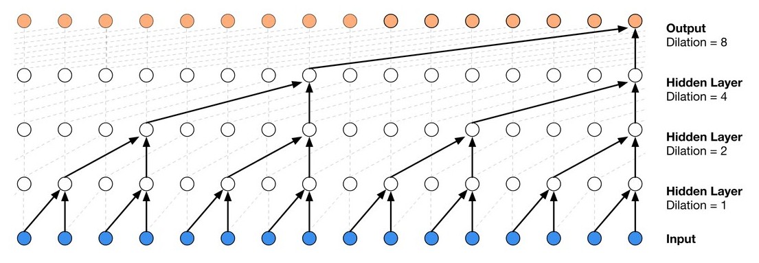
Figure 1: Visualisation of a WaveNet stack and its receptive field [27].

图 1：WaveNet 堆叠及其感受野的示意 [27]。

Raw audio data is typically very high-dimensional (e.g. 16,000 samples per second for 16kHz audio), and contains complex, hierarchical structures spanning many thousands of time steps, such as words in speech or melodies in music. Modelling such long-term dependencies with standard causal convolution layers would require a very deep network to ensure a sufficiently broad receptive field. WaveNet avoids this constraint by using dilated causal convolutions, which allow the receptive field to grow exponentially with depth.

原始音频数据通常维数非常高（例如 16 kHz 音频每秒有 16,000 个采样点），并且包含跨越数千个时间步的复杂层次结构，比如语音里的词，或音乐里的旋律。若用标准的因果卷积层去建模这样的长期依赖，网络必须非常深，才能保证感受野足够宽。WaveNet 用膨胀因果卷积避开了这一限制，从而让感受野随深度指数增长。

WaveNet uses gated activation functions, together with a simple mechanism introduced in [19] to condition on extra information such as class labels or linguistic features:

WaveNet 使用门控激活函数，并采用 [19] 中提出的一种简单机制，以便对类别标签或语言学特征这类额外信息做条件化：

$$\bm{h}_{i}=\sigma\left(W_{g,i}\ast\bm{x}_{i}+V_{g,i}^{T}\bm{c}\right)\odot\tanh\left(W_{f,i}\ast\bm{x}_{i}+V_{f,i}^{T}\bm{c}\right), \tag{1}$$

where $\ast$ denotes a convolution operator, and $\odot$ denotes an element-wise multiplication operator. $\sigma(\cdot)$ is a logistic sigmoid function. $\bm{c}$ represents extra conditioning data. $i$ is the layer index. $f$ and $g$ denote filter and gate, respectively. $W$ and $V$ are learnable weights. In cases where $\bm{c}$ encodes spatial or sequential information (such as a sequence of linguistic features), the matrix products ($V_{f,i}^{T}\bm{c}$ and $V_{g,i}^{T}\bm{c}$) are replaced by convolutions ($V_{f,i}\ast\bm{c}$ and $V_{g,i}\ast\bm{c}$).

其中 $\ast$ 表示卷积运算，$\odot$ 表示逐元素相乘。$\sigma(\cdot)$ 是逻辑斯谛 sigmoid 函数。$\bm{c}$ 表示额外的条件数据。$i$ 是层的编号。$f$ 和 $g$ 分别表示滤波器和门。$W$ 和 $V$ 是可学习的权重。当 $\bm{c}$ 编码的是空间或序列信息（例如一串语言学特征）时，矩阵乘积（$V_{f,i}^{T}\bm{c}$ 和 $V_{g,i}^{T}\bm{c}$）会被换成卷积（$V_{f,i}\ast\bm{c}$ 和 $V_{g,i}\ast\bm{c}$）。

2.1 Higher Fidelity WaveNet

2.1 更高保真度的 WaveNet

For this work we made two improvements to the basic WaveNet model to enhance its audio quality for production use. Unlike previous versions of WaveNet [27], where 8-bit ($\mu$-law or PCM) audio was modelled with a 256-way categorical distribution, we increased the fidelity by modelling 16-bit audio. Since training a 65,536-way categorical distribution would be prohibitively costly, we instead modelled the samples with the discretized mixture of logistics distribution introduced in [23]. We further improved fidelity by increasing the audio sampling rate from 16kHz to 24kHz. This required a WaveNet with a wider receptive field, which we achieved by increasing the dilated convolution filter size from 2 to 3. An alternative strategy would be to increase the number of layers or add more dilation stages.

为了这项工作，我们对基本的 WaveNet 模型做了两处改进，以提高它在生产使用中的音频保真度。此前的 WaveNet 版本 [27] 用 256 类的分类分布来建模 8 比特（$\mu$-law 或 PCM）音频；我们改为建模 16 比特音频，从而提高了保真度。训练一个 65,536 类的分类分布代价过高，因此我们改用 [23] 中提出的离散化逻辑斯谛混合分布来建模采样点。我们还把音频采样率从 16 kHz 提高到 24 kHz，进一步改善了保真度。这要求 WaveNet 有更宽的感受野，我们把膨胀卷积的滤波器尺寸从 2 加大到 3 来实现这一点。另一种策略是增加层数，或再加若干膨胀阶段。

3 Parallel WaveNet

3 并行 WaveNet

While the convolutional structure of WaveNet allows for rapid parallel training, sample generation remains inherently sequential and therefore slow, as it is for all autoregressive models which use ancestral sampling. We therefore seek an alternative architecture that will allow for rapid, parallel generation.

WaveNet 的卷积结构允许快速的并行训练，但样本生成本质上仍是顺序的，因此很慢，所有使用祖先采样的自回归模型都是如此。于是我们寻求一种能够快速、并行生成的替代结构。

Inverse-autoregressive flows (IAFs) [15] are stochastic generative models whose latent variables are arranged so that all elements of a high dimensional observable sample can be generated in parallel. IAFs are a special type of normalising flow [3, 22, 4] which model a multivariate distribution $p_{X}(\bm{x})$ as an explicit invertible non-linear transformation $f$ of a simple tractable distribution $p_{Z}(\bm{z})$ (such as an isotropic Gaussian distribution). The resulting random variable $\bm{x}=f(\bm{z})$ has a log probability:

逆自回归流（IAF） [15] 是一类随机生成模型，其潜变量的安排使得高维可观测样本的所有元素都可以并行生成。IAF 是一种特殊的归一化流（normalising flow） [3, 22, 4]，它把多元分布 $p_{X}(\bm{x})$ 建模成一个简单、易于处理的分布 $p_{Z}(\bm{z})$（例如各向同性高斯分布）经过显式可逆非线性变换 $f$ 之后的结果。得到的随机变量 $\bm{x}=f(\bm{z})$ 具有对数概率：

$$\log p_{X}(\bm{x})=\log p_{Z}(\bm{z})-\log\Big|\frac{d\bm{x}}{d\bm{z}}\Big|,$$

where $\big|\frac{d\bm{x}}{d\bm{z}}\big|$ is the determinant of the Jacobian of $f$. The transformation $f$ is typically chosen so that it is invertible and its Jacobian determinant is easy to compute. In the case of an IAF, $x_{t}$ is modelled by $p(x_{t}|\bm{z}_{\leq t})$ so that $x_{t}=f(\bm{z}_{\leq t})$. The transformation has a triangular Jacobian matrix which makes the determinant simply the product of the diagonal entries:

其中 $\big|\frac{d\bm{x}}{d\bm{z}}\big|$ 是 $f$ 的雅可比行列式。变换 $f$ 通常选成可逆的，并且其雅可比行列式易于计算。在 IAF 的情形下，$x_{t}$ 由 $p(x_{t}|\bm{z}_{\leq t})$ 建模，从而 $x_{t}=f(\bm{z}_{\leq t})$。这个变换的雅可比矩阵是三角的，于是行列式就是对角元的乘积：

$$\log\Big|\frac{d\bm{x}}{d\bm{z}}\Big|=\sum_{t}\log\frac{\partial f(\bm{z}_{\leq t})}{\partial z_{t}}.$$

Initially, a random sample is drawn from $\bm{z}\sim\mathrm{Logistic}(0,I)$. The following transformation is applied to $\bm{z}$:

一开始，先从 $\bm{z}\sim\mathrm{Logistic}(0,I)$ 中抽取一个随机样本。然后对 $\bm{z}$ 施加如下变换：

$$\displaystyle x_{t}=z_{t}\cdot s(\bm{z}_{<t},\bm{\theta})+\mu(\bm{z}_{<t},\bm{\theta}) \tag{2}$$

The network outputs a sample $\bm{x}$, as well as $\bm{\mu}$ and $\bm{s}$. Therefore, $p(x_{t}|\bm{z}_{<t})$ follows a logistic distribution parameterised by $\mu_{t}$ and $s_{t}$.

网络输出一个样本 $\bm{x}$，以及 $\bm{\mu}$ 和 $\bm{s}$。因此，$p(x_{t}|\bm{z}_{<t})$ 服从由 $\mu_{t}$ 和 $s_{t}$ 参数化的逻辑斯谛分布。

$$p(x_{t}|\bm{z}_{<t},\bm{\theta})=\mathop{\mathbb{L}}\left(x_{t}\big|\mu(\bm{z}_{<t},\bm{\theta}),s(\bm{z}_{<t},\bm{\theta})\right),$$

While $\mu(\bm{z}_{<t},\bm{\theta})$ and $s(\bm{z}_{<t},\bm{\theta})$ can be any autoregressive model, we use the same convolutional autoregressive network structure as the original WaveNet [27]. If an IAF and an autoregressive model share the same output distribution class (e.g., mixture of logistics or categorical) then mathematically they should be able to model the same multivariate distributions. However, in practice there are some differences (see Appendix section A.2). To output the correct distribution for timestep $x_{t}$, the inverse autoregressive flow can implicitly infer what it would have output at previous timesteps $x_{1},\dots,x_{t-1}$ based on the noise inputs $z_{1},\dots,z_{t-1}$, which allows it to output all $x_{t}$ in parallel given $z_{t}$.

虽然 $\mu(\bm{z}_{<t},\bm{\theta})$ 和 $s(\bm{z}_{<t},\bm{\theta})$ 可以是任意自回归模型，我们使用的是与原来 WaveNet [27] 相同的卷积自回归网络结构。如果 IAF 和自回归模型共享同一类输出分布（例如逻辑斯谛混合或分类分布），那么从数学上讲它们应当能够建模相同的多元分布。不过在实践中仍有一些差别（见附录 A.2 节）。为了给出时间步 $x_{t}$ 上正确的分布，逆自回归流可以根据噪声输入 $z_{1},\dots,z_{t-1}$，隐式推断它在前面的时间步 $x_{1},\dots,x_{t-1}$ 上会输出什么，从而在给定 $z_{t}$ 时并行输出所有 $x_{t}$。

In general, normalising flows might require repeated iterations to transform uncorrelated noise into structured samples, with the output generated by the flow at each iteration passed in as input at the next [22] one. This is less crucial for IAFs, as the autoregressive latents can induce significant structure in a single pass. Nonetheless we observed that having up to 4 flow iterations (which we implemented by simply stacking 4 such networks on top of each other) did improve the quality. Note that in the final parallel WaveNet architecture, the weights were not shared between the flows.

一般而言，归一化流可能需要反复迭代，才能把不相关的噪声变成有结构的样本，每一轮流生成的输出会作为下一轮的输入 [22]。对 IAF 来说这一点不那么关键，因为自回归的潜变量可以在单次遍历中就诱导出可观的结构。尽管如此，我们观察到最多使用 4 次流迭代（我们的实现就是简单地把 4 个这样的网络叠在一起）确实提高了质量。需要说明的是，在最终的并行 WaveNet 结构里，各流之间并不共享权重。

The first (bottom) network takes as input the white unconditional logistic noise: $\bm{x}^{0}=\bm{z}$. Thereafter the output of each network $i$ is passed as input to the next network $i+1$ , which again transforms it.

最下面的第一个网络以无条件的白色逻辑斯谛噪声作为输入：$\bm{x}^{0}=\bm{z}$。此后，每个网络 $i$ 的输出被送到下一个网络 $i+1$ 作为输入，再做一次变换。

$$\displaystyle\bm{x}^{i} \\ \displaystyle=\bm{x^{i-1}}\cdot\bm{s}^{i}+\bm{\mu}^{i} \tag{3}$$

Because we use the same ordering in all the flows, the final distribution $p(x_{t}|z_{<t},\bm{\theta})$ is logistic with location $\mu_{\text{tot}}$ and scale $s_{\text{tot}}$:

因为我们在所有流中使用相同的变量顺序，最终分布 $p(x_{t}|z_{<t},\bm{\theta})$ 是位置为 $\mu_{\text{tot}}$、尺度为 $s_{\text{tot}}$ 的逻辑斯谛分布：

$$\displaystyle\bm{\mu}_{\text{tot}} \\ \displaystyle=\sum_{i}^{N}\bm{\mu}^{i}\left(\prod_{j>i}^{N}\bm{s}^{j}\right) \\ \displaystyle\bm{s}_{\text{tot}} \\ \displaystyle=\prod_{i}^{N}\bm{s}_{i} \tag{4}$$

where $N$ is the number of flows and the dependencies on $t$ and $z$ are omitted for simplicity.

其中 $N$ 是流的个数，对 $t$ 和 $z$ 的依赖为简洁起见略去。

4 Probability Density Distillation

4 概率密度蒸馏

Training the parallel WaveNet model directly with maximum likelihood would be impractical, as the inference procedure required to estimate the log-likelihoods is sequential and slow[^1]. We therefore introduce a novel form of neural network distillation [11] that uses an already trained WaveNet as a ‘teacher’ from which a parallel WaveNet ‘student’ can efficiently learn. To stress the fact that we are dealing with normalised density models, we refer to this process as Probability Density Distillation (in contrast to Probability Density Estimation). The basic idea is for the student to attempt to match the probability of its own samples under the distribution learned by the teacher.

[^1]: In this sense the two architectures are dual to one another: slow training and fast generation with parallel WaveNet versus fast training and slow generation with WaveNet.

若直接用最大似然训练并行 WaveNet 模型，并不实际，因为估计对数似然所需的推断过程是顺序的、很慢[^1]。因此我们提出一种新的神经网络蒸馏 [11]：用已经训练好的 WaveNet 作为“老师”，让并行 WaveNet“学生”能够高效地学习。为了强调我们处理的是已经归一化的密度模型，我们把这个过程称为 概率密度蒸馏（以区别于概率密度估计）。基本想法是：让学生努力使自己样本在老师所学分布下的概率与老师相匹配。

[^1]：在这个意义上，两种结构是对偶的：并行 WaveNet 训练慢、生成快，原来的 WaveNet 则训练快、生成慢。

Given a parallel WaveNet student $p_{S}(\bm{x})$ and WaveNet teacher $p_{T}(\bm{x})$ which has been trained on a dataset of audio, we define the Probability Density Distillation loss as follows:

给定一个并行 WaveNet 学生 $p_{S}(\bm{x})$，以及一个已经在音频数据集上训练好的 WaveNet 老师 $p_{T}(\bm{x})$，我们把 概率密度蒸馏 损失定义如下：

$$D_{\text{KL}}\left(P_{S}||P_{T}\right)=H(P_{S},P_{T})-H(P_{S}) \tag{6}$$

where $D_{\text{KL}}$ is the Kullback–Leibler divergence, and $H(P_{S},P_{T})$ is the cross-entropy between the student $P_{S}$ and teacher $P_{T}$, and $H(P_{S})$ is the entropy of the student distribution. When the KL divergence becomes zero, the student distribution has fully recovered the teacher’s distribution. The entropy term (which is not present in previous distillation objectives [11]) is vital in that it prevents the student’s distribution from collapsing to the mode of the teacher (which, counter-intuitively, does not yield a good sample—see Appendix section A.1). Crucially, all the operations required to estimate derivatives for this loss (sampling from $p_{S}(\bm{x})$, evaluating $p_{T}(\bm{x})$, and evaluating $H(P_{S})$) can be performed efficiently, as we will see.

其中 $D_{\text{KL}}$ 是 Kullback–Leibler 散度，$H(P_{S},P_{T})$ 是学生 $P_{S}$ 与老师 $P_{T}$ 之间的交叉熵，$H(P_{S})$ 是学生分布的熵。当 KL 散度变为零时，学生分布已经完全恢复了老师的分布。熵这一项（以往的蒸馏目标里并没有 [11]）至关重要：它防止学生的分布塌缩到老师的众数上（与直觉相反，那样并不会得到好的样本——见附录 A.1 节）。关键的是，估计这个损失的导数所需的全部运算（从 $p_{S}(\bm{x})$ 采样、评估 $p_{T}(\bm{x})$，以及评估 $H(P_{S})$）都可以高效完成，下面就会看到。

It is worth noting the parallels to Generative Adversarial Networks (GANs [7]), with the student playing the role of generator, and the teacher playing the role of discriminator. As opposed to GANs, however, the student is not attempting to fool the teacher in an adversarial manner; rather it co-operates by attempting to match the teacher’s probabilities. Furthermore the teacher is held constant, rather than being trained in tandem with the student, and both models yield tractable normalised distributions.

值得注意的是，这与生成对抗网络（GAN [7]）有平行之处：学生扮演生成器的角色，老师扮演判别器的角色。不过与 GAN 不同，学生并不是以对抗的方式去欺骗老师；相反，它通过努力匹配老师的概率来配合老师。此外，老师是固定的，而不是与学生一起训练；而且两个模型都给出可处理的归一化分布。

Recently [9] has presented a related idea to train feed-forward networks for neural machine translation. Their method is based on conditioning the feedforward decoder on fertility values, which require supervision by an external alignment system. The training procedure also involves the creation of an additional dataset as well as fine-tuning. During inference, their model relies on re-scoring by an auto-regressive model.

最近，[9] 提出了一个相关想法，用于训练神经机器翻译中的前馈网络。他们的方法基于用生育率（fertility）值来条件化前馈解码器，而这需要由外部对齐系统来提供监督。训练过程还涉及构造一个额外的数据集以及微调。在推断时，他们的模型依赖于用自回归模型再打一遍分。

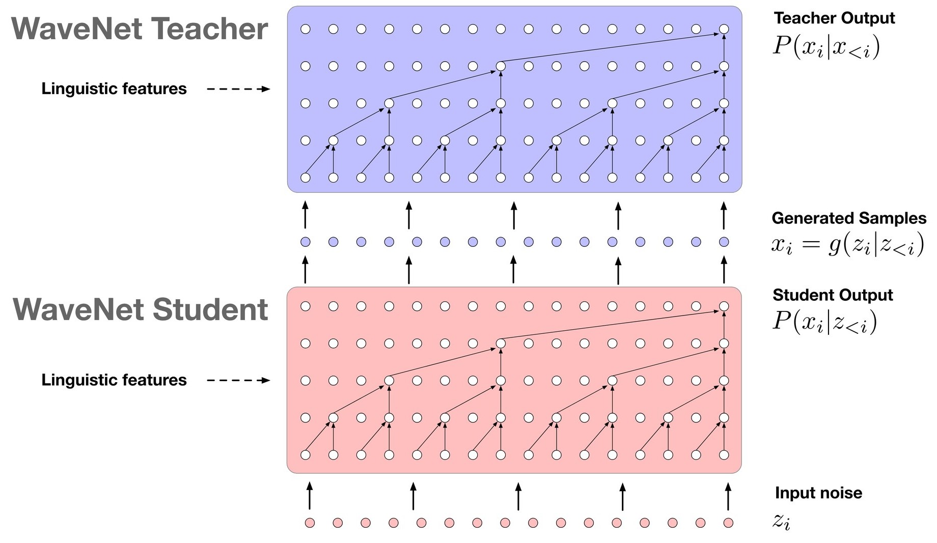
Figure 2: Overview of Probability Density Distillation. A pre-trained WaveNet teacher is used to score the samples $\bm{x}$ output by the student. The student is trained to minimise the KL-divergence between its distribution and that of the teacher by maximising the log-likelihood of its samples under the teacher and maximising its own entropy at the same time.

图 2：概率密度蒸馏概览。预训练好的 WaveNet 老师用来对学生输出的样本 $\bm{x}$ 打分。学生的训练目标是最小化自己的分布与老师分布之间的 KL 散度：一方面最大化其样本在老师下的对数似然，另一方面同时最大化自身的熵。

First, observe that the entropy term $H(P_{S})$ in Equation 6 can be rewritten as follows:

首先可以看到，方程 6 中的熵项 $H(P_{S})$ 可以改写成：

$$\displaystyle H(P_{S}) \\ \displaystyle=\mathop{\mathbb{E}}_{z\sim L(0,1)}\left[\sum_{t=1}^{T}-\ln p_{S}(x_{t}|\bm{z}_{<t})\right] \\ \displaystyle=\mathop{\mathbb{E}}_{z\sim L(0,1)}\left[\sum_{t=1}^{T}\ln s(\bm{z}_{<t},\bm{\theta})\right]+2T, \tag{7}$$

where $\bm{x}=g(\bm{z})$ and $z_{t}$ are independent samples drawn from the logistic distribution. The second equality in Equation 8 follows because the entropy of a logistic distribution $\mathop{\mathbb{L}}(\mu,s)$ is $\ln s+2$. We can therefore compute this term without having to explicitly generate $\bm{x}$.

其中 $\bm{x}=g(\bm{z})$，而 $z_{t}$ 是从逻辑斯谛分布中独立抽出的样本。方程 8 中的第二个等式之所以成立，是因为逻辑斯谛分布 $\mathop{\mathbb{L}}(\mu,s)$ 的熵是 $\ln s+2$。因此我们可以计算这一项，而不必显式生成 $\bm{x}$。

The cross-entropy term $H(P_{S},P_{T})$ however explicitly depends on $\bm{x}=g(\bm{z})$, and therefore requires sampling from the student to estimate.

不过，交叉熵项 $H(P_{S},P_{T})$ 明确依赖于 $\bm{x}=g(\bm{z})$，因此需要从学生中采样才能估计。

$$\displaystyle H(P_{S},P_{T}) \\ \displaystyle=\int_{\bm{x}}p_{S}(\bm{x})\ln p_{T}(\bm{x}) \\ \displaystyle=\sum_{t=1}^{T}\int_{\bm{x}}p_{S}(\bm{x})\ln p_{T}(x_{t}|\bm{x}_{<t}) \\ \displaystyle=\sum_{t=1}^{T}\int_{\bm{x}}p_{S}(\bm{x}_{<t})p_{S}(x_{t}|\bm{x}_{<t})p_{S}(\bm{x}_{>t}|\bm{x}_{\leq t})\ln p_{T}(x_{t}|\bm{x}_{<t}) \\ \displaystyle=\sum_{t=1}^{T}\mathop{\mathbb{E}}_{p_{S}(\bm{x}_{<t})}\bigg[\int_{x_{t}}p_{S}(x_{t}|\bm{x}_{<t})\ln p_{T}(x_{t}|\bm{x}_{<t})\int_{\bm{x}_{>t}}p_{S}(\bm{x}_{>t}|\bm{x}_{\leq t})\bigg] \\ \displaystyle=\sum_{t=1}^{T}\mathop{\mathbb{E}}_{p_{S}(\bm{x}_{<t})}H\Big(p_{S}(x_{t}|\bm{x}_{<t}),p_{T}(x_{t}|\bm{x}_{<t})\Big). \tag{9}$$

For every sample $\bm{x}$ we draw from the student $p_{S}$ we can compute all $p_{T}(x_{t}|\bm{x}_{<t})$ in parallel with the teacher and then evaluate $H(p_{S}(x_{t}|\bm{x}_{<t}),p_{T}(x_{t}|\bm{x}_{<t}))$ very efficiently by drawing multiple different samples $x_{t}$ from $p_{S}(x_{t}|\bm{x}_{<t})$ for each timestep. This unbiased estimator has a much lower variance than naively evaluating the sample under the teacher with Equation 9.

对从学生 $p_{S}$ 抽出的每一个样本 $\bm{x}$，我们可以与老师一起并行算出所有 $p_{T}(x_{t}|\bm{x}_{<t})$，再通过在每个时间步从 $p_{S}(x_{t}|\bm{x}_{<t})$ 中抽取多个不同的 $x_{t}$，非常高效地评估 $H(p_{S}(x_{t}|\bm{x}_{<t}),p_{T}(x_{t}|\bm{x}_{<t}))$。与用方程 9 把样本直接放到老师下面评估相比，这个无偏估计量的方差要低得多。

Because the teacher’s output distribution $p_{T}(x_{t}|\bm{x}_{<t})$ is parameterised as a mixture of logistics distribution, the loss term $\ln p_{T}(x_{t}|\bm{x}_{<t})$ is differentiable with respect to both $x_{t}$ and $x_{<t}$. A categorical distribution, on the other hand, would only be differentiable w.r.t. $\bm{x}_{<t}$.

因为老师的输出分布 $p_{T}(x_{t}|\bm{x}_{<t})$ 被参数化成逻辑斯谛混合分布，损失项 $\ln p_{T}(x_{t}|\bm{x}_{<t})$ 对 $x_{t}$ 和 $x_{<t}$ 都可微。若改用分类分布，则只对 $\bm{x}_{<t}$ 可微。

4.1 Additional loss terms

4.1 额外的损失项

Training with Probability Density Distillation alone might not sufficiently constrain the student to generate high quality audio streams. Therefore, we also introduce additional loss functions to guide the student distribution towards the desired output space.

如果只靠 概率密度蒸馏 来训练，可能还不足以约束学生生成高质量的音频流。因此我们再引入一些额外的损失函数，把学生分布导向想要的输出空间。

Power loss

The first additional loss we propose is the power loss, which ensures that the power in different frequency bands of the speech are on average used as much as in human speech. The power loss helps to avoid the student from collapsing to a high-entropy WaveNet-mode, such as whispering.

功率损失

我们提出的第一项额外损失是 功率损失，它保证语音在不同频带上的功率，平均而言用得和人类语音一样多。功率损失有助于避免学生塌缩到一种高熵的 WaveNet 模式，例如耳语。

The power-loss is defined as:

功率损失定义为：

$$||\phi(g(\bm{z},\bm{c}))-\phi(\bm{y})||^{2}, \tag{14}$$

where $(\bm{y},\bm{c})$ is an example with conditioning from the training set, $\phi(\bm{x})=|\text{STFT}(\bm{x})|^{2}$ and STFT stands for the Short-Term Fourier Transform. We found that $\phi(\bm{x})$ can be averaged over time before taking the Euclidean distance with little difference in effect, which means it is the average power for various frequencies that is important.

其中 $(\bm{y},\bm{c})$ 是训练集中的一个带条件信息的例子，$\phi(\bm{x})=|\text{STFT}(\bm{x})|^{2}$，STFT 表示短时傅里叶变换。我们发现，在取欧氏距离之前先对 $\phi(\bm{x})$ 做时间平均，效果几乎没有差别，这说明重要的是各频率上的平均功率。

Perceptual loss

In the power loss formulation given in equation 14, one can also use a neural network instead of the STFT to conserve a perceptual property of the signal rather than total energy. In our case we have used a WaveNet-like classifier trained to predict the phones from raw audio. Because such a classifier naturally extracts high-level features that are relevant for recognising the phones, this loss term penalises bad pronunciations. A similar principle has been used in computer vision for artistic style transfer [5], or to get better perceptual reconstruction losses, e.g., in super-resolution [12].

感知损失

在方程 14 给出的功率损失形式里，也可以用神经网络代替 STFT，以保持信号的某种感知性质，而不是总能量。在我们的情形中，使用的是一个 WaveNet 式的分类器，训练来从原始音频预测音素。这样的分类器会自然提取出对识别音素有关的高层特征，因此这一损失项会惩罚发音不好的样本。计算机视觉里也用过类似原则，例如艺术风格迁移 [5]，或在超分辨率中得到更好的感知重建损失 [12]。

We have experimented with two different ways of using the perceptual loss, the feature reconstruction loss (the Euclidean distance between feature maps in the classifier) and the style loss (the Euclidean distance between the Gram matrices [12]). The latter produced better results in our experiments.

我们试验过两种使用感知损失的方式：特征重建损失（分类器中特征图之间的欧氏距离）和风格损失（Gram 矩阵之间的欧氏距离 [12]）。在我们的实验里，后者效果更好。

Contrastive loss

Finally, we also introduce a contrastive distillation loss as follows:

对比损失

最后，我们还引入如下的对比蒸馏损失：

$$D_{\text{KL}}\Big(P_{S}(\bm{c}_{1})\Big|\Big|P_{T}(\bm{c}_{1})\Big)-\gamma D_{\text{KL}}\Big(P_{S}(\bm{c}_{1})\Big|\Big|P_{T}\bm{c}_{2})\Big), \tag{15}$$

which minimises the KL-divergence between the teacher and student when both are conditioned on the same information $\bm{c}_{1}$ (e.g., linguistic features, speaker ID, …), but also maximises it for different conditioning pairs $\bm{c}1\neq\bm{c}2$. In order to implement this loss, we use the output of the student $\bm{x}=g(\bm{z},\bm{c}_{1})$ and evaluate the waveform twice under the teacher: once with the same conditioning $P_{T}(\bm{x}|\bm{c}_{1})$ and once with a randomly sampled conditioning input: $P_{T}(\bm{x}|\bm{c}_{2})$. The weight for the contrastive term $\gamma$ was set to 0.3 in our experiments. The contrastive loss penalises waveforms that have high likelihood regardless of the conditioning vector.

它在老师和学生都条件于同一信息 $\bm{c}_{1}$（例如语言学特征、说话人 ID 等）时最小化两者的 KL 散度，同时在不同的条件对 $\bm{c}_{1}\neq\bm{c}_{2}$ 上最大化 KL 散度。为实现这一损失，我们使用学生的输出 $\bm{x}=g(\bm{z},\bm{c}_{1})$，并在老师下对这段波形评估两次：一次使用相同的条件 $P_{T}(\bm{x}|\bm{c}_{1})$，一次使用随机抽取的条件输入 $P_{T}(\bm{x}|\bm{c}_{2})$。实验中对比项的权重 $\gamma$ 设为 0.3。对比损失会惩罚那些无论条件向量是什么都具有高似然的波形。

5 Experiments

5 实验

In all our experiments we used text-to-speech models that were conditioned on linguistic features (similar to [27]), providing phonetic and duration information to the network. We also conditioned the models on pitch information (logarithm of $f_{0}$, the fundamental frequency) predicted by a different model. We never used ground-truth information (such as pitch or duration) extracted from human speech for generating audio samples and the test sentences were not present (or similar to those) in the training set.

在所有实验中，我们使用的文本转语音模型都以语言学特征为条件（与 [27] 类似），向网络提供音素和时长信息。我们还用另一个模型预测的音高信息（基频 $f_{0}$ 的对数）来条件化这些模型。生成音频样本时，我们从不使用从人类语音中提取的真值信息（例如音高或时长），测试句子也不在训练集中出现（或与之相似）。

The teacher WaveNet network was trained for 1,000,000 steps with the ADAM optimiser [14] with a minibatch size of 32 audio clips, each containing 7,680 timesteps (roughly 320ms). Remarkably, a relatively short snippet of time is sufficient to train the parallel WaveNet to produce long term coherent waveforms. The learning rate was held constant at $2\times 10^{-4}$, and Polyak averaging [21] was applied over the parameters. The model consists of 30 layers, grouped into 3 dilated residual block stacks of 10 layers. In every stack, the dilation rate increases by a factor of 2 in every layer, starting with rate 1 (no dilation) and reaching the maximum dilation of 512 in the last layer. The filter size of causal dilated convolutions is 3. The number of hidden units in the gating layers is 512 (split into two groups of 256 for the two parts of the activation function (1)). The number of hidden units in the residual connection is 512, and in the skip connection and the $1\times 1$ convolutions before the output layer is also 256. We used 10 mixture components for the mixture of logistics output distribution.

老师 WaveNet 网络用 ADAM 优化器 [14] 训练了 1,000,000 步，minibatch 大小为 32 段音频，每段包含 7,680 个时间步（大约 320 毫秒）。值得注意的是，相对较短的时间片段就足以训练并行 WaveNet，使之生成具有长期一致性的波形。学习率固定为 $2\times 10^{-4}$，并对参数做 Polyak 平均 [21]。模型共 30 层，分成 3 组膨胀残差块堆，每堆 10 层。在每一堆中，膨胀率在每一层增大 2 倍，从 1（不膨胀）开始，到最后一层达到最大膨胀率 512。因果膨胀卷积的滤波器尺寸为 3。门控层的隐单元数是 512（按激活函数 (1) 的两个部分分成两组，每组 256）。残差连接中的隐单元数是 512，跳跃连接以及输出层之前的 $1\times 1$ 卷积中的隐单元数是 256。逻辑斯谛混合输出分布使用了 10 个混合分量。

The student network consisted of the same WaveNet architecture layout, except with different inputs and outputs and no skip connections. The student was also trained for 1,000,000 steps with the same optimisation settings. The student typically consisted of 4 flows with 10, 10, 10, 30 layers respectively, with 64 hidden units for the residual and gating layers.

学生网络采用与 WaveNet 相同的结构布局，只是输入和输出不同，并且没有跳跃连接。学生同样用相同的优化设置训练了 1,000,000 步。学生通常由 4 个流组成，层数依次为 10、10、10 与 30，残差层和门控层的隐单元数为 64。

Audio Generation Speed

We have benchmarked the sampling speed of autoregressive and distilled WaveNets on an NVIDIA P100 GPU. Both models were implemented in Tensorflow [1] and compiled with XLA. The hidden layer activations from previous timesteps in the autoregressive model were cached with circular buffers [20]. The resulting sampling speed with this implementation is 172 timesteps/second for a minibatch of size 1. The distilled model, which is more parallelizable, achieves over 500,000 timesteps/second with same batch size of 1, resulting in three orders of magnitude speed-up.

音频生成速度

我们在一块 NVIDIA P100 GPU 上对自回归 WaveNet 和蒸馏后的 WaveNet 的采样速度做了基准测试。两个模型都在 Tensorflow [1] 中实现，并用 XLA 编译。自回归模型中前一时间步的隐层激活用环形缓冲来缓存 [20]。在这种实现下，minibatch 大小为 1 时的采样速度是 172 个时间步/秒。蒸馏后的模型更易于并行，在同样 batch 大小为 1 时达到 超过 500,000 个时间步/秒，从而带来三个数量级的加速。

Method	Subjective 5-scale MOS
16kHz, 8-bit $\bm{\mu}$-law, 25h data:
LSTM-RNN parametric [27]	3.67 $\pm$ 0.098
HMM-driven concatenative [27]	3.86 $\pm$ 0.137
WaveNet [27]	4.21 $\pm$ 0.081
24kHz, 16-bit linear PCM, 65h data:
HMM-driven concatenative	4.19 $\pm$ 0.097
Autoregressive WaveNet	4.41 $\pm$ 0.069
Distilled WaveNet	4.41 $\pm$ 0.078

Table 1: Comparison of WaveNet distillation with the autoregressive teacher WaveNet, unit-selection (concatenative), and previous results from [27]. MOS stands for Mean Opinion Score.

方法	主观 5 分制 MOS
16 kHz，8 比特 $\bm{\mu}$-law，25 小时数据：
LSTM-RNN 参数系统 [27]	3.67 $\pm$ 0.098
HMM 驱动的拼接系统 [27]	3.86 $\pm$ 0.137
WaveNet [27]	4.21 $\pm$ 0.081
24 kHz，16 比特线性 PCM，65 小时数据：
HMM 驱动的拼接系统	4.19 $\pm$ 0.097
自回归 WaveNet	4.41 $\pm$ 0.069
蒸馏 WaveNet	4.41 $\pm$ 0.078

表 1：把 WaveNet 蒸馏与自回归的老师 WaveNet、单元选择（拼接）系统，以及 [27] 中以往结果相对照。MOS 表示平均意见分（Mean Opinion Score）。

Audio Fidelity

In our first set of experiments, we looked at the quality of WaveNet distillation compared to the autoregressive WaveNet teacher and other baselines on data from a professional female speaker [27]. Table 1 gives a comparison of autoregressive WaveNet, distilled WaveNet and current production systems in terms of mean opinion score (MOS). There is no difference between MOS scores of the distilled WaveNet ($4.41\pm 0.08$) and autoregressive WaveNet ($4.41\pm 0.07$), and both are significantly better than the concatenative unit-selection baseline ($4.19\pm 0.1$).

音频保真度

在第一组实验里，我们在一位专业女声的数据上 [27]，考察了 WaveNet 蒸馏相对于自回归 WaveNet 老师以及其他基线的质量。表 1 从平均意见分（MOS）的角度对照了自回归 WaveNet、蒸馏 WaveNet 和当时的生产系统。蒸馏 WaveNet（$4.41\pm 0.08$）与自回归 WaveNet（$4.41\pm 0.07$）的 MOS 没有差别，并且都显著好于拼接式单元选择基线（$4.19\pm 0.1$）。

It is also important to note that the difference in MOS scores of our WaveNet baseline result $4.41$ compared to the previous reported result $4.21$ [27] is due to the improvement in audio fidelity as explained in Section 2.1: modelling a sample rate of $24$kHz instead of $16$kHz and bit-depth of $16$-bit PCM instead of $8$-bit $\mu$-law.

还需要说明的是，我们的 WaveNet 基线结果 $4.41$ 与此前报告的 $4.21$ [27] 之间的 MOS 差别，来自第 2.1 节所解释的保真度提升：把采样率从 $16$ kHz 改成 $24$ kHz，并把位深从 8 比特 $\mu$-law 改成 16 比特 PCM。

	Parametric	Concatenative	Distilled WaveNet
English speaker 1 (female - 65h data)	3.88	4.19	4.41
English speaker 2 (male - 21h data)	3.96	4.09	4.34
English speaker 3 (male - 10h data)	3.77	3.65	4.47
English speaker 4 (female - 9h data)	3.42	3.40	3.97
Japanese speaker (female - 28h data)	4.07	3.47	4.23

Table 2: Comparison of MOS scores on English and Japanese with multi-speaker distilled WaveNets. Note that some speakers sounded less appealing to people and always get lower MOS, however distilled parallel WaveNet always achieved significantly better results.

	参数系统	拼接系统	蒸馏 WaveNet
英语说话人 1（女声，65 小时数据）	3.88	4.19	4.41
英语说话人 2（男声，21 小时数据）	3.96	4.09	4.34
英语说话人 3（男声，10 小时数据）	3.77	3.65	4.47
英语说话人 4（女声，9 小时数据）	3.42	3.40	3.97
日语说话人（女声，28 小时数据）	4.07	3.47	4.23

表 2：用多说话人蒸馏 WaveNet，在英语和日语上对照 MOS。需要说明的是，有些说话人听起来不太讨人喜欢，MOS 总会偏低，但蒸馏后的并行 WaveNet 始终取得了明显更好的结果。

Multi-speaker Generation

By conditioning on the speaker-ids we can construct a single parallel WaveNet model that is able to generate multiple speakers’ voices and their accents. These networks require slightly more capacity than single speaker models and thus had 30 layers in each flow. In Table 2 we show a comparison of such a distilled parallel WaveNet model with two main baselines: a parametric and a concatenative system. In the comparison, we use a number of English speakers from a single model (one of them, English speaker 1, is the same speaker as in Table 1) and a Japanese speaker from another model. For some speakers, the concatenative system gets better results than the parametric system, while for other speakers it is the opposite. The parallel WaveNet model, on the other hand, significantly outperforms both baselines for all the speakers.

多说话人生成

通过对说话人 ID 做条件化，我们可以构造一个单独的并行 WaveNet 模型，生成多位说话人的声音及其口音。这些网络比单说话人模型需要稍多一些容量，因此每个流有 30 层。表 2 把这样一个蒸馏后的并行 WaveNet 模型与两个主要基线相对照：一个参数系统和一个拼接系统。对照中，我们使用来自同一个模型的若干英语说话人（其中英语说话人 1 与表 1 中的是同一位），以及来自另一个模型的一位日语说话人。对有些说话人，拼接系统比参数系统更好；对另一些说话人则正好相反。另一方面，并行 WaveNet 模型在所有说话人都显著优于这两个基线。

Ablation Studies

	Preference Scores
	versus baseline concatenative system
Method	Win - Lose - Neutral
Losses used
KL + Power	60% - 15% - 25%
KL + Power + Perceptual	66% - 10% - 24%
KL + Power + Perceptual + Contrastive (= default)	65% - 9% - 26%

Table 3: Performance with respect to different combinations of loss terms. We report preference comparison scores since their mean opinion scores tend to be very close and inconclusive.

消融实验

	偏好分数
	相对基线拼接系统
方法	胜 - 负 - 中立
所用损失
KL + 功率	60% - 15% - 25%
KL + 功率 + 感知	66% - 10% - 24%
KL + 功率 + 感知 + 对比（= 默认）	65% - 9% - 26%

表 3：不同损失项组合下的表现。我们报告偏好对照分数，因为这些模型的平均意见分往往非常接近，难以得出结论。

To analyse the importance of the loss functions introduced in Section 4.1 we show how the quality of the distilled WaveNet changes with different loss functions in Table 3 (top). We found that MOS scores of these models tend to be very similar to each other (and similar to the result in Table 1). Therefore, we report subjective preference scores from a paired comparison test (“A/B test”), which we found to be more reliable for noticing small (sometimes qualitative) differences. In these tests, the subjects were asked to listen to a pair of samples and choose which they preferred, though they could choose “neutral” if they did not have any preference.

为了分析第 4.1 节引入的损失函数有多重要，我们在表 3（上半部分）中展示蒸馏 WaveNet 的质量如何随不同损失函数变化。我们发现这些模型的 MOS 往往彼此非常接近（也接近表 1 中的结果）。因此我们报告配对比较测试（“A/B 测试”）中的主观偏好分数，我们发现它对察觉细小（有时是性质上的）差别更为可靠。在这些测试中，受试者被要求听一对样本并选出更喜欢的那一个，如果没有任何偏好，也可以选择“中立”。

As mentioned before, the KL loss alone does not constrain the distillation process enough to obtain natural sounding speech (e.g., low-volume audio suffices for the KL), therefore we do not report preference scores with only this term. The KL loss (section  4) combined with power-loss is enough to generate quite natural speech. Adding the perceptual loss gives a small but noticeable improvement. Adding the contrastive loss does not improve the preference scores any further, but makes the generated speech less noisy, which is something most raters do not pay attention to, but is important for production quality speech.

如前所述，只靠 KL 损失还不足以约束蒸馏过程，得到听起来自然的语音（例如，音量很低的音频就足以应付 KL），因此我们不报告只含这一项时的偏好分数。把 KL 损失（第 4 节）与功率损失结合起来，已经足以生成相当自然的语音。再加上感知损失，会带来虽小但可以察觉的改进。再加入对比损失并不会让偏好分数进一步提高，但会让生成的语音不那么嘈杂；多数评分人未必注意这一点，对生产质量的语音却很重要。

As explained in Section 3, we use multiple inverse-autoregressive flows in the parallel WaveNet architecture: A model with a single flow gets a MOS score of 4.21, compared to a MOS score of 4.41 for models with multiple flows.

如第 3 节所解释的，我们在并行 WaveNet 结构中使用多个逆自回归流：只有单个流的模型 MOS 为 4.21，而具有多个流的模型 MOS 为 4.41。

6 Conclusion

6 结论

In this paper we have introduced a novel method for high-fidelity speech synthesis based on WaveNet [27] using Probability Density Distillation. The proposed model achieved several orders of magnitude speed-up compared to the original WaveNet with no significant difference in quality. Moreover, we have successfully transferred this algorithm to new languages and multiple speakers.

本文提出了一种基于 WaveNet [27]、使用 概率密度蒸馏 的高保真语音合成新方法。与原来的 WaveNet 相比，所提出的模型实现了几个数量级的加速，音质没有明显差别。此外，我们已成功把这一算法迁移到新的语言和多名说话人上。

The resulting system has been deployed in production at Google, and is currently being used to serve Google Assistant queries in real time to millions of users^2. We believe that the same method presented here can be used in many different domains to achieve similar speed improvements whilst maintaining output accuracy.

得到的系统已在 Google 的生产环境中部署，目前正被用来实时服务数百万用户的 Google Assistant 查询[^2]。我们相信，这里给出的同一方法也可以用在许多不同领域，在保持输出精度的同时获得类似的速度提升。

[^2]：https://deepmind.com/blog/wavenet-launches-google-assistant/

7 Acknowledgements

7 致谢

In this paper, we have described the research advances that made it possible for WaveNet to meet the speed and quality requirements for being used in production at Google. At the same time, an equivalently significant effort has gone into integrating this new end-to-end deep learning model into the production pipeline, satisfying requirements of not only speed, but latency and reliability, among others. We would like to thank Ben Coppin, Edgar Duéñez-Guzmán, Akihiro Matsukawa, Lizhao Liu, Mahalia Miller, Trevor Strohman and Eddie Kessler for very useful discussions. We also would like to thank the entire DeepMind Applied and Google Speech teams for their foundational contributions to the project and developing the production pipeline.

在本文中，我们描述了使 WaveNet 满足 Google 生产使用在速度和音质上要求的那些研究进展。与此同时，把这个新的端到端深度学习模型接入生产流水线，并满足速度之外的延迟、可靠性等要求，也同样花费了巨大努力。我们要感谢 Ben Coppin、Edgar Duéñez-Guzmán、Akihiro Matsukawa、Lizhao Liu、Mahalia Miller、Trevor Strohman 和 Eddie Kessler 非常有益的讨论。我们也要感谢整个 DeepMind Applied 团队和 Google Speech 团队，感谢他们对本项目的基础性贡献，以及生产流水线的开发。

References

参考文献

[1] Martín Abadi, Ashish Agarwal, Paul Barham, Eugene Brevdo, Zhifeng Chen, Craig Citro, Greg S Corrado, Andy Davis, Jeffrey Dean, Matthieu Devin, et al. Tensorflow: Large-scale machine learning on heterogeneous distributed systems. arXiv preprint arXiv:1603.04467 , 2016.

[2] Xi Chen, Diederik P Kingma, Tim Salimans, Yan Duan, Prafulla Dhariwal, John Schulman, Ilya Sutskever, and Pieter Abbeel. Variational lossy autoencoder. arXiv preprint arXiv:1611.02731 , 2016.

[3] Laurent Dinh, David Krueger, and Yoshua Bengio. Nice: Non-linear independent components estimation. arXiv preprint arXiv:1410.8516 , 2014.

[4] Laurent Dinh, Jascha Sohl-Dickstein, and Samy Bengio. Density estimation using real nvp. arXiv preprint arXiv:1605.08803 , 2016.

[5] Leon A Gatys, Alexander S Ecker, and Matthias Bethge. A neural algorithm of artistic style. arXiv preprint arXiv:1508.06576 , 2015.

[6] Mathieu Germain, Karol Gregor, Iain Murray, and Hugo Larochelle. Made: masked autoencoder for distribution estimation. In Proceedings of the 32nd International Conference on Machine Learning (ICML-15) , pages 881–889, 2015.

[7] Ian Goodfellow, Jean Pouget-Abadie, Mehdi Mirza, Bing Xu, David Warde-Farley, Sherjil Ozair, Aaron Courville, and Yoshua Bengio. Generative adversarial nets. In Advances in neural information processing systems , pages 2672–2680, 2014.

[8] Alex Graves. Generating sequences with recurrent neural networks. arXiv preprint arXiv:1308.0850 , 2013.

[9] Jiatao Gu, James Bradbury, Caiming Xiong, Victor OK Li, and Richard Socher. Non-autoregressive neural machine translation. arXiv preprint arXiv:1711.02281 , 2017.

[10] Geoffrey Hinton, Li Deng, Dong Yu, George E Dahl, Abdel-rahman Mohamed, Navdeep Jaitly, Andrew Senior, Vincent Vanhoucke, Patrick Nguyen, Tara N Sainath, et al. Deep neural networks for acoustic modeling in speech recognition: The shared views of four research groups. IEEE Signal Processing Magazine , 29(6):82–97, 2012.

[11] Geoffrey Hinton, Oriol Vinyals, and Jeff Dean. Distilling the knowledge in a neural network. arXiv preprint arXiv:1503.02531 , 2015.

[12] Justin Johnson, Alexandre Alahi, and Li Fei-Fei. Perceptual losses for real-time style transfer and super-resolution. In European Conference on Computer Vision , pages 694–711. Springer, 2016.

[13] Nal Kalchbrenner, Aaron van den Oord, Karen Simonyan, Ivo Danihelka, Oriol Vinyals, Alex Graves, and Koray Kavukcuoglu. Video pixel networks. arXiv preprint arXiv:1610.00527 , 2016.

[14] Diederik Kingma and Jimmy Ba. Adam: A method for stochastic optimization. arXiv preprint arXiv:1412.6980 , 2014.

[15] Diederik P Kingma, Tim Salimans, and Max Welling. Improving variational inference with inverse autoregressive flow. arXiv preprint arXiv:1606.04934 , 2016.

[16] Alex Krizhevsky, Ilya Sutskever, and Geoffrey E Hinton. Imagenet classification with deep convolutional neural networks. In Advances in neural information processing systems , pages 1097–1105, 2012.

[17] Hugo Larochelle and Iain Murray. The neural autoregressive distribution estimator. In Proceedings of the Fourteenth International Conference on Artificial Intelligence and Statistics , pages 29–37, 2011.

[18] Tomas Mikolov, Martin Karafiát, Lukas Burget, Jan Cernockỳ, and Sanjeev Khudanpur. Recurrent neural network based language model. In Interspeech , volume 2, page 3, 2010.

[19] Aaron van den Oord, Nal Kalchbrenner, and Koray Kavukcuoglu. Pixel recurrent neural networks. arXiv preprint arXiv:1601.06759 , 2016.

[20] Tom Le Paine, Pooya Khorrami, Shiyu Chang, Yang Zhang, Prajit Ramachandran, Mark A. Hasegawa-Johnson, and Thomas S. Huang. Fast wavenet generation algorithm. CoRR , abs/1611.09482, 2016.

[21] Boris T Polyak and Anatoli B Juditsky. Acceleration of stochastic approximation by averaging. SIAM Journal on Control and Optimization , 30(4):838–855, 1992.

[22] Danilo Jimenez Rezende and Shakir Mohamed. Variational inference with normalizing flows. arXiv preprint arXiv:1505.05770 , 2015.

[23] Tim Salimans, Andrej Karpathy, Xi Chen, and Diederik P Kingma. Pixelcnn++: Improving the pixelcnn with discretized logistic mixture likelihood and other modifications. arXiv preprint arXiv:1701.05517 , 2017.

[24] Casper Kaae Sønderby, Jose Caballero, Lucas Theis, Wenzhe Shi, and Ferenc Huszár. Amortised map inference for image super-resolution. arXiv preprint arXiv:1610.04490 , 2016.

[25] Christian Szegedy, Wei Liu, Yangqing Jia, Pierre Sermanet, Scott Reed, Dragomir Anguelov, Dumitru Erhan, Vincent Vanhoucke, and Andrew Rabinovich. Going deeper with convolutions. In Proceedings of the IEEE conference on computer vision and pattern recognition , pages 1–9, 2015.

[26] Lucas Theis and Matthias Bethge. Generative image modeling using spatial lstms. In Advances in Neural Information Processing Systems , pages 1927–1935, 2015.

[27] Aaron van den Oord, Sander Dieleman, Heiga Zen, Karen Simonyan, Oriol Vinyals, Alex Graves, Nal Kalchbrenner, Andrew Senior, and Koray Kavukcuoglu. Wavenet: A generative model for raw audio. arXiv preprint arXiv:1609.03499 , 2016.

[28] Aaron van den Oord, Nal Kalchbrenner, Lasse Espeholt, Oriol Vinyals, Alex Graves, et al. Conditional image generation with pixelcnn decoders. In Advances in Neural Information Processing Systems , pages 4790–4798, 2016.

[29] Yonghui Wu, Mike Schuster, Zhifeng Chen, Quoc V Le, Mohammad Norouzi, Wolfgang Macherey, Maxim Krikun, Yuan Cao, Qin Gao, Klaus Macherey, et al. Google’s neural machine translation system: Bridging the gap between human and machine translation. arXiv preprint arXiv:1609.08144 , 2016.

Appendix A Appendix

附录 A 附录

A.1 Argument against MAP estimation

A.1 反对 MAP 估计的一个论证

In this section we make an argument against maximum a posteriori (MAP) estimation for distillation; similar arguments have been made by previous authors in a different setting [24].

在这一节里，我们给出一个反对把 最大后验（MAP）估计用于蒸馏的论证；以往作者在不同设定下也提出过类似论点 [24]。

The distillation loss defined in Section 4 minimises the KL divergence between the teacher and generator. We could instead have minimised only the cross-entropy between the teacher and generator (the standard distillation loss term [11]), so that the samples by the generator are as likely as possible according to the teacher. Doing so would give rise to MAP estimation. Counter-intuitively, audio samples obtained through MAP estimation do not sound as good as typical examples from the teacher: in fact they are almost completely silent, even if using conditional information such as linguistic features. This effect is not due to adversarial behaviour on the part of the teacher, but rather is a fundamental property of the data distribution which the teacher has approximated.

第 4 节定义的蒸馏损失最小化的是老师和生成器之间的 KL 散度。我们本来也可以只最小化老师和生成器之间的交叉熵（也就是标准的蒸馏损失项 [11]），从而使生成器给出的样本在老师看来尽可能地像。那样做就会变成 MAP 估计。与直觉相反，通过 MAP 估计得到的音频样本听起来并不如老师的典型样本好：实际上它们几乎完全是静音的，即便使用了语言学特征这类条件信息也是如此。这个效应并不是因为老师在做对抗，而是老师所逼近的数据分布的一个基本性质。

As an example consider the simple case where we have audio from a white random noise source: the distribution at every timestep is $\mathcal{N}(0,1)$, regardless of the samples at previous timesteps. White noise has a very specific and perceptually recognizable sound: a continual hiss. The MAP estimate of this data distribution, and thus of any generative model that matches it well, recovers the distribution mode, which is 0 at every timestep: i.e. complete silence. More generally, any highly stochastic process is liable to have a ‘noiseless’ and therefore atypical mode. For the KL divergence the optimum is to recover the full teacher distribution. This is clearly different from any random sample from the distribution. Furthermore, if one changes the representation of the data (e.g., by nonlinearly pre-processing the audio signal), then the MAP estimate changes, unlike the KL-divergence in Equation 6, which is invariant to the coordinate system.

举一个简单的例子：假设音频来自白噪声源，那么每个时间步上的分布都是 $\mathcal{N}(0,1)$，与前面时间步的样本无关。白噪声有一种非常特定、在感知上很容易辨认的声音：持续的嘶声。对这个数据分布（以及任何与之匹配得很好的生成模型）做 MAP 估计，得到的是分布的众数，也就是每个时间步都是 0：即完全静音。更一般地说，任何高度随机的过程都容易有一个“无噪声”、因而并不典型的众数。对 KL 散度而言，最优是恢复老师的完整分布。这显然不同于该分布的任意一个随机样本。此外，如果改变数据的表示（例如对音频信号做非线性预处理），MAP 估计会随之改变；而方程 6 中的 KL 散度对坐标系是不变的。

A.2 Autoregressive Models and Inverse-autoregressive Flows

A.2 自回归模型与逆自回归流

Although inverse-autoregressive flows (IAFs) and autoregressive models can in principle model the same distributions [2], they have different inductive biases and may vary greatly in their capacity to model certain processes. As a simple example consider the Fibonacci series $(1,1,2,3,5,8,13,\dots)$. For an autoregressive model this is easy to model with a receptive field of two: $f(k)=f(k-1)+f(k-2)$. For an IAF, however, the receptive field needs to be at least size $k$ to correctly model $k$ terms, leading to a larger model that is less able to generalise.

尽管逆自回归流（IAF）和自回归模型原则上可以建模相同的分布 [2]，它们具有不同的归纳偏置，对某些过程的建模能力可能相差很大。一个简单的例子是斐波那契数列 $(1,1,2,3,5,8,13,\dots)$。对自回归模型来说，用大小为 2 的感受野就很容易建模：$f(k)=f(k-1)+f(k-2)$。对 IAF 来说，要正确建模 $k$ 项，感受野至少需要达到 $k$，从而模型更大，也更不容易泛化。