ORB-SLAM: A Versatile and Accurate Monocular SLAM System
This paper has been accepted for publication in IEEE Transactions on Robotics.
DOI: 10.1109/TRO.2015.2463671
IEEE Xplore: http://ieeexplore.ieee.org/xpl/articleDetails.jsp?arnumber=7219438
©2015 IEEE. Personal use of this material is permitted. Permission from IEEE must be obtained for all other uses, in any current or future media, including reprinting/republishing this material for advertising or promotional purposes, creating new collective works, for resale or redistribution to servers or lists, or reuse of any copyrighted component of this work in other works.
arXiv:1502.00956v2 [cs.RO] 18 Sep 2015
本文已被 IEEE Transactions on Robotics 接收发表。
DOI: 10.1109/TRO.2015.2463671
IEEE Xplore: http://ieeexplore.ieee.org/xpl/articleDetails.jsp?arnumber=7219438
©2015 IEEE。允许个人使用本材料。若在当前或未来的任何媒体中将本材料用于广告或宣传目的的重印/再发表、创作新的汇编作品、转售或再分发至服务器或列表,或在其他作品中重用本作品的任何受版权保护部分,必须获得 IEEE 的许可。
arXiv:1502.00956v2 [cs.RO] 18 Sep 2015
ORB-SLAM: a Versatile and Accurate Monocular SLAM System
Raúl Mur-Artal*, J. M. M. Montiel, Member, IEEE, and Juan D. Tardós, Member, IEEE
The authors are with the Instituto de Investigación en Ingeniería de Aragón (I3A), Universidad de Zaragoza, María de Luna 1, 50018 Zaragoza, Spain (e-mail: raulmur@unizar.es; josemari@unizar.es; tardos@unizar.es).
- Corresponding author.
This work was supported by the Dirección General de Investigación of Spain under Project DPI2012-32168, the Ministerio de Educación Scholarship FPU13/04175 and Gobierno de Aragón Scholarship B121/13.
Abstract
This paper presents ORB-SLAM, a feature-based monocular SLAM system that operates in real time, in small and large, indoor and outdoor environments. The system is robust to severe motion clutter, allows wide baseline loop closing and relocalization, and includes full automatic initialization. Building on excellent algorithms of recent years, we designed from scratch a novel system that uses the same features for all SLAM tasks: tracking, mapping, relocalization, and loop closing. A survival of the fittest strategy that selects the points and keyframes of the reconstruction leads to excellent robustness and generates a compact and trackable map that only grows if the scene content changes, allowing lifelong operation. We present an exhaustive evaluation in 27 sequences from the most popular datasets. ORB-SLAM achieves unprecedented performance with respect to other state-of-the-art monocular SLAM approaches. For the benefit of the community, we make the source code public.
本文提出 ORB-SLAM,一套基于特征的单目 SLAM 系统,可在小场景和大场景、室内和室外环境中实时运行。该系统对严重的运动混乱具有鲁棒性,允许宽基线回环闭合和重定位,并包含完全自动的初始化。在近年优秀算法的基础上,我们从零设计了一套新系统,对所有 SLAM 任务使用同一特征:跟踪、建图、重定位和回环闭合。一种选择重建中的点和关键帧的“适者生存”策略带来了出色的鲁棒性,并生成紧凑、可跟踪的地图;地图只在场景内容发生变化时才增长,从而允许长期运行。我们在最常用数据集中的 27 条序列上做了详尽评估。相对于其他当时最先进的单目 SLAM 方法,ORB-SLAM 取得了前所未有的表现。为便于社区使用,我们将源代码公开。
Index Terms—Lifelong Mapping, Localization, Monocular Vision, Recognition, SLAM
I. INTRODUCTION
Bundle Adjustment (BA) is known to provide accurate estimates of camera localizations as well as a sparse geometrical reconstruction [1], [2], given that a strong network of matches and good initial guesses are provided. For long time this approach was considered unaffordable for real time applications such as Visual Simultaneous Localisation and Mapping (Visual SLAM). Visual SLAM has the goal of estimating the camera trajectory while reconstructing the environment. Nowadays we know that to achieve accurate results at non-prohibitive computational cost, a real time SLAM algorithm has to provide BA with:
已知在具有牢固的匹配网络和良好初值的前提下,束调整(BA)能够给出精确的相机定位估计以及稀疏几何重建 [1], [2]。在很长一段时间里,这种方法被认为无法用于视觉同时定位与地图构建(Visual SLAM)这类实时应用。Visual SLAM 的目标是在重建环境的同时估计相机轨迹。现在我们知道,要在计算代价可承受的前提下得到精确结果,实时 SLAM 算法必须为 BA 提供:
- corresponding observations of scene features (map points) among a subset of selected frames (keyframes).
- 在所选帧(关键帧)的一个子集之间,对场景特征(地图点)的对应观测。
- As complexity grows with the number of keyframes, their selection should avoid unnecessary redundancy.
- 由于复杂度随关键帧数量增长,关键帧的选择应避免不必要的冗余。
- A strong network configuration of keyframes and points to produce accurate results, that is, a well spread set of keyframes observing points with significant parallax and with plenty of loop closure matches.
- 关键帧与点的牢固网络配置,以产生精确结果,也就是一组分布良好的关键帧,它们观测具有显著视差的点,并带有大量回环匹配。
- An initial estimation of the keyframe poses and point locations for the non-linear optimization.
- 供非线性优化使用的关键帧位姿和点位置的初始估计。
- A local map in exploration where optimization is focused to achieve scalability.
- 在探索过程中使用局部地图,把优化集中在局部,以实现可扩展性。
- The ability to perform fast global optimizations (e.g. pose graph) to close loops in real-time.
- 能够进行快速的全局优化(例如位姿图),以便实时闭合回环。
The first real time application of BA was the visual odometry work of Mouragon et. al. [3], followed by the ground breaking SLAM work of Klein and Murray [4], known as Parallel Tracking and Mapping (PTAM). This algorithm, while limited to small scale operation, provides simple but effective methods for keyframe selection, feature matching, point triangulation, camera localization for every frame, and relocalization after tracking failure. Unfortunately several factors severely limit its application: lack of loop closing and adequate handling of occlusions, low invariance to viewpoint of the relocalization and the need of human intervention for map bootstrapping.
BA 的第一个实时应用是 Mouragon et. al. [3] 的视觉里程计工作,随后是 Klein 和 Murray [4] 开创性的 SLAM 工作,即并行跟踪与建图(PTAM)。该算法虽然限于小规模运行,但为关键帧选择、特征匹配、点三角化、每一帧的相机定位,以及跟踪失败后的重定位提供了简单而有效的方法。不幸的是,若干因素严重限制了它的应用:缺少回环闭合和对遮挡的充分处理,重定位对视角变化的不变性较低,以及地图启动需要人工介入。
In this work we build on the main ideas of PTAM, the place recognition work of Gálvez-López and Tardós [5], the scale-aware loop closing of Strasdat et. al [6] and the use of covisibility information for large scale operation [7], [8], to design from scratch ORB-SLAM, a novel monocular SLAM system whose main contributions are:
在本工作中,我们以 PTAM 的主要思想、Gálvez-López 和 Tardós [5] 的位置识别工作、Strasdat et. al [6] 对尺度敏感的回环闭合,以及共视信息在大规模运行中的使用 [7], [8] 为基础,从零设计 ORB-SLAM,一套新颖的单目 SLAM 系统,其主要贡献是:
- Use of the same features for all tasks: tracking, mapping, relocalization and loop closing. This makes our system more efficient, simple and reliable. We use ORB features [9] which allow real-time performance without GPUs, providing good invariance to changes in viewpoint and illumination.
- 对所有任务使用同一特征:跟踪、建图、重定位和回环闭合。这使我们的系统更高效、简单和可靠。我们使用 ORB 特征 [9],它无需 GPU 即可实时运行,并对视角和光照变化具有良好的不变性。
- Real time operation in large environments. Thanks to the use of a covisibility graph, tracking and mapping is focused in a local covisible area, independent of global map size.
- 在大型环境中实时运行。由于使用了共视图,跟踪和建图集中在局部共视区域,与全局地图大小无关。
- Real time loop closing based on the optimization of a pose graph that we call the Essential Graph. It is built from a spanning tree maintained by the system, loop closure links and strong edges from the covisibility graph.
- 基于我们称为 Essential Graph 的位姿图优化,实现实时回环闭合。该图由系统维护的生成树、回环闭合链接以及来自共视图的强边构成。
- Real time camera relocalization with significant invariance to viewpoint and illumination. This allows recovery from tracking failure and also enhances map reuse.
- 对视角和光照具有显著不变性的实时相机重定位。这允许从跟踪失败中恢复,也增强了地图的复用。
- A new automatic and robust initialization procedure based on model selection that permits to create an initial map of planar and non-planar scenes.
- 一种基于模型选择的新的自动且鲁棒的初始化程序,能够为平面和非平面场景创建初始地图。
- A survival of the fittest approach to map point and keyframe selection that is generous in the spawning but very restrictive in the culling. This policy improves tracking robustness, and enhances lifelong operation because redundant keyframes are discarded.
- 一种针对地图点和关键帧选择的“适者生存”方法,在生成时较为慷慨,但在裁减时非常严格。这一策略提高了跟踪鲁棒性,并通过丢弃冗余关键帧增强了长期运行能力。
We present an extensive evaluation in popular public datasets from indoor and outdoor environments, including hand-held, car and robot sequences. Notably, we achieve better camera localization accuracy than the state of the art in direct methods [10], which optimize directly over pixel intensities instead of feature reprojection errors. We include a discussion in Section IX-B on the possible causes that can make feature-based methods more accurate than direct methods.
我们在来自室内和室外环境的常用公开数据集上做了广泛评估,包括手持、车载和机器人序列。值得注意的是,我们取得了比当时最先进的直接法 [10] 更好的相机定位精度,后者直接对像素强度而不是特征重投影误差进行优化。我们在第 IX-B 节讨论了可能使基于特征的方法比直接法更精确的原因。
The loop closing and relocalization methods here presented are based on our previous work [11]. A preliminary version of the system was presented in [12]. In the current paper we add the initialization method, the Essential Graph, and perfect all methods involved. We also describe in detail all building blocks and perform an exhaustive experimental validation. To the best of our knowledge, this is the most complete and reliable solution to monocular SLAM, and for the benefit of the community we make the source code public. Demonstration videos and the code can be found in our project webpage.
这里给出的回环闭合和重定位方法基于我们此前的工作 [11]。该系统的一个初步版本曾在 [12] 中介绍。在本文中,我们加入了初始化方法和 Essential Graph,并完善了所涉及的全部方法。我们还详细描述了所有构建模块,并做了详尽的实验验证。据我们所知,这是当时最完整、最可靠的单目 SLAM 解决方案,为便于社区使用,我们将源代码公开。演示视频和代码可在我们的项目网页上找到。
II. RELATED WORK
A. Place Recognition
The survey by Williams et al. [13] compared several approaches for place recognition and concluded that techniques based on appearance, that is image to image matching, scale better in large environments than map to map or image to map methods. Within appearance based methods, bags of words techniques [14], such as the probabilistic approach FAB-MAP [15], are to the fore because of their high efficiency. DBoW2 [5] used for the first time bags of binary words obtained from BRIEF descriptors [16] along with the very efficient FAST feature detector [17]. This reduced in more than one order of magnitude the time needed for feature extraction, compared to SURF [18] and SIFT [19] features that were used in bags of words approaches so far. Although the system demonstrated to be very efficient and robust, the use of BRIEF, neither rotation nor scale invariant, limited the system to in-plane trajectories and loop detection from similar viewpoints.
Williams et al. [13] 的综述比较了若干位置识别方法,并认为基于外观的技术,也就是图像到图像的匹配,在大型环境中比地图到地图或图像到地图的方法更易扩展。在基于外观的方法中,词袋技术 [14],例如概率方法 FAB-MAP [15],因其高效而处于前列。DBoW2 [5] 首次使用由 BRIEF 描述子 [16] 得到的二进制词袋,并配合非常高效的 FAST 特征检测器 [17]。与此前词袋方法中使用的 SURF [18] 和 SIFT [19] 特征相比,这把特征提取所需时间降低了一个数量级以上。尽管该系统被证明非常高效且鲁棒,但 BRIEF 既没有旋转不变性也没有尺度不变性,把系统限制在平面内轨迹以及从相近视角检测回环。
In our previous work [11], we proposed a bag of words place recognizer built on DBoW2 with ORB [9]. ORB are binary features invariant to rotation and scale (in a certain range), resulting in a very fast recognizer with good invariance to viewpoint. We demonstrated the high recall and robustness of the recognizer in four different datasets, requiring less than 39ms (including feature extraction) to retrieve a loop candidate from a 10K image database. In this work we use an improved version of that place recognizer, using covisibility information and returning several hypotheses when querying the database instead of just the best match.
在我们此前的工作 [11] 中,我们提出了一种建立在 DBoW2 之上、使用 ORB [9] 的词袋位置识别器。ORB 是在一定范围内对旋转和尺度不变的二进制特征,从而得到一个非常快、对视角具有良好不变性的识别器。我们在四个不同数据集上证明了该识别器的高召回和鲁棒性,从 1 万张图像的数据库中检索一个回环候选(包括特征提取)所需时间不到 39ms。在本工作中,我们使用该位置识别器的改进版本,利用共视信息,并在查询数据库时返回多个假设,而不只是最佳匹配。
B. Map Initialization
Monocular SLAM requires a procedure to create an initial map because depth cannot be recovered from a single image. One way to solve the problem is to initially track a known structure [20]. In the context of filtering approaches, points can be initialized with high uncertainty in depth using an inverse depth parametrization [21], which hopefully will later converge to their real positions. The recent semi-dense work of Engel et al. [10], follows a similar approach initializing the depth of the pixels to a random value with high variance.
单目 SLAM 需要一套创建初始地图的程序,因为无法从单张图像恢复深度。一种解决办法是一开始跟踪已知结构 [20]。在滤波方法中,可以用逆深度参数化 [21] 以很高的深度不确定性初始化点,并希望它们随后收敛到真实位置。Engel et al. [10] 近期的半稠密工作采取了类似做法,把像素深度初始化为方差很大的随机值。
Initialization methods from two views either assumes locally scene planarity [4], [22] and recover the relative camera pose from a homography using the method of Faugeras et. al [23], or compute an essential matrix [24], [25] that models planar and general scenes, using the five-point algorithm of Nister [26], which requires to deal with multiple solutions. Both reconstruction methods are not well constrained under low parallax and suffer from a twofold ambiguity solution if all points of a planar scene are closer to one of the camera centers [27]. On the other hand if a non-planar scene is seen with parallax a unique fundamental matrix can be computed with the eight-point algorithm [2] and the relative camera pose can be recovered without ambiguity.
从两视图初始化的方法,或者局部假定场景共面 [4], [22],并用 Faugeras et. al [23] 的方法从单应恢复相对相机位姿,或者计算能够同时刻画平面和一般场景的本质矩阵 [24], [25],使用 Nister [26] 的五点算法,这需要处理多个解。这两种重建方法在小视差下都约束不足;若平面场景中的所有点都更靠近其中一个相机中心,还会出现双重歧义解 [27]。另一方面,如果非平面场景是在有视差的情况下被看到的,就可以用八点算法 [2] 计算出唯一的基本矩阵,并无歧义地恢复相对相机位姿。
We present in Section IV a new automatic approach based on model selection between a homography for planar scenes and a fundamental matrix for non-planar scenes. A statistical approach to model selection was proposed by Torr et al. [28]. Under a similar rationale we have developed a heuristic initialization algorithm that takes into account the risk of selecting a fundamental matrix in close to degenerate cases (i.e. planar, nearly planar, and low parallax), favoring the selection of the homography. In the planar case, for the sake of safe operation, we refrain from initializing if the solution has a twofold ambiguity, as a corrupted solution could be selected. We delay the initialization until the method produces a unique solution with significant parallax.
我们在第 IV 节提出一种新的自动方法,在用于平面场景的单应和用于非平面场景的基本矩阵之间做模型选择。Torr et al. [28] 曾提出一种统计的模型选择方法。在类似思路下,我们开发了一种启发式初始化算法,它考虑了在接近退化的情形(即平面、接近平面,以及小视差)下选择基本矩阵的风险,从而更倾向于选择单应。在平面情形中,为了安全运行,如果解具有双重歧义,我们就暂不初始化,因为可能选出被污染的解。我们把初始化推迟到该方法产生具有显著视差的唯一解为止。
C. Monocular SLAM
Monocular SLAM was initially solved by filtering [20], [21], [29], [30]. In that approach every frame is processed by the filter to jointly estimate the map feature locations and the camera pose. It has the drawbacks of wasting computation in processing consecutive frames with little new information and the accumulation of linearization errors. On the other hand keyframe-based approaches [3], [4] estimate the map using only selected frames (keyframes) allowing to perform more costly but accurate bundle adjustment optimizations, as mapping is not tied to frame-rate. Strasdat et. al [31] demonstrated that keyframe-based techniques are more accurate than filtering for the same computational cost.
单目 SLAM 最初是用滤波方法解决的 [20], [21], [29], [30]。在那种做法里,每一帧都由滤波器处理,以联合估计地图特征位置和相机位姿。其缺点是:在几乎没有新信息的连续帧上浪费计算,以及线性化误差会累积。另一方面,基于关键帧的方法 [3], [4] 只用所选帧(关键帧)估计地图,从而可以进行代价更高但更精确的束调整优化,因为建图不必绑在帧率上。Strasdat et. al [31] 证明,在相同计算代价下,基于关键帧的技术比滤波更精确。
The most representative keyframe-based SLAM system is probably PTAM by Klein and Murray [4]. It was the first work to introduce the idea of splitting camera tracking and mapping in parallel threads, and demonstrated to be successful for real time augmented reality applications in small environments. The original version was later improved with edge features, a rotation estimation step during tracking and a better relocalization method [32]. The map points of PTAM correspond to FAST corners matched by patch correlation. This makes the points only useful for tracking but not for place recognition. In fact PTAM does not detect large loops, and the relocalization is based on the correlation of low resolution thumbnails of the keyframes, yielding a low invariance to viewpoint.
最有代表性的基于关键帧的 SLAM 系统,大概是 Klein 和 Murray [4] 的 PTAM。它首次提出把相机跟踪和建图分到并行线程中,并在小环境的实时增强现实应用中取得了成功。原版后来又用边缘特征、跟踪中的旋转估计步骤以及更好的重定位方法做了改进 [32]。PTAM 的地图点对应于用块相关匹配的 FAST 角点。这使得这些点只对跟踪有用,而不能用于位置识别。事实上 PTAM 不检测大回环,重定位基于关键帧低分辨率缩略图的相关,对视角变化的不变性较低。
Strasdat et. al [6] presented a large scale monocular SLAM system with a front-end based on optical flow implemented on a GPU, followed by FAST feature matching and motion-only BA, and a back-end based on sliding-window BA. Loop closures were solved with a pose graph optimization with similarity constraints (7DoF), that was able to correct the scale drift appearing in monocular SLAM. From this work we take the idea of loop closing with 7DoF pose graph optimization and apply it to the Essential Graph defined in Section III-D.
Strasdat et. al [6] 提出一套大规模单目 SLAM 系统,其前端基于在 GPU 上实现的光流,随后是 FAST 特征匹配和仅运动 BA,后端则基于滑动窗口 BA。回环用带相似约束(7DoF)的位姿图优化来解决,能够校正单目 SLAM 中出现的尺度漂移。我们从这项工作中吸取用 7DoF 位姿图优化做回环的想法,并把它应用到第 III-D 节定义的 Essential Graph 上。
Strasdat et. al [7] used the front-end of PTAM, but performed the tracking only in a local map retrieved from a covisibility graph. They proposed a double window optimization back-end that continuously performs BA in the inner window, and pose graph in a limited-size outer window. However, loop closing is only effective if the size of the outer window is large enough to include the whole loop. In our system we take advantage of the excellent ideas of using a local map based on covisibility, and building the pose graph from the covisibility graph, but apply them in a totally redesigned front-end and back-end. Another difference is that, instead of using specific features for loop detection (SURF), we perform the place recognition on the same tracked and mapped features, obtaining robust frame-rate relocalization and loop detection.
Strasdat et. al [7] 使用了 PTAM 的前端,但只在从共视图检索到的局部地图中进行跟踪。他们提出一种双窗口优化后端,在内窗口中持续做 BA,并在大小受限的外窗口中做位姿图优化。然而,只有当外窗口大到足以包含整个回环时,回环闭合才有效。在我们的系统中,我们利用了基于共视的局部地图,以及从共视图构建位姿图这些优秀想法,但把它们用在完全重新设计的前端和后端中。另一个区别是,我们不是为回环检测使用专门的特征(SURF),而是在同一套被跟踪和建图的特征上做位置识别,从而得到鲁棒的帧率重定位和回环检测。
Pirker et. al [33] proposed CD-SLAM, a very complete system including loop closing, relocalization, large scale operation and efforts to work on dynamic environments. However map initialization is not mentioned. The lack of a public implementation does not allow us to perform a comparison of accuracy, robustness or large-scale capabilities.
Pirker et. al [33] 提出了 CD-SLAM,一套非常完整的系统,包括回环闭合、重定位、大规模运行,以及在动态环境中工作的尝试。不过论文没有提及地图初始化。由于缺少公开实现,我们无法对其精度、鲁棒性或大规模能力进行比较。
The visual odometry of Song et al. [34] uses ORB features for tracking and a temporal sliding window BA back-end. In comparison our system is more general as they do not have global relocalization, loop closing and do not reuse the map. They are also using the known distance from the camera to the ground to limit monocular scale drift.
Song et al. [34] 的视觉里程计使用 ORB 特征进行跟踪,并以时间滑动窗口 BA 为后端。相比之下,我们的系统更一般,因为他们没有全局重定位和回环闭合,也不复用地图。他们还使用相机到地面的已知距离来限制单目尺度漂移。
Lim et. al [25], work published after we submitted our preliminary version of this work [12], use also the same features for tracking, mapping and loop detection. However the choice of BRIEF limits the system to in-plane trajectories. Their system only tracks points from the last keyframe so the map is not reused if revisited (similar to visual odometry) and has the problem of growing unbounded. We compare qualitatively our results with this approach in section VIII-E.
Lim et. al [25] 的工作是在我们提交本工作的初步版本 [12] 之后发表的,他们也对跟踪、建图和回环检测使用同一特征。然而选择 BRIEF 把系统限制在平面内轨迹。他们的系统只跟踪来自上一关键帧的点,因此在再次访问时不复用地图(类似于视觉里程计),并存在无限增长的问题。我们在第 VIII-E 节与这一方法做了定性比较。
The recent work of Engel et. al [10], known as LSD-SLAM, is able to build large scale semi-dense maps, using direct methods (i.e. optimization directly over image pixel intensities) instead of bundle adjustment over features. Their results are very impressive as the system is able to operate in real time, without GPU acceleration, building a semi-dense map, with more potential applications for robotics than the sparse output generated by feature-based SLAM. Nevertheless they still need features for loop detection and their camera localization accuracy is significantly lower than in our system and PTAM, as we show experimentally in Section VIII-B. This surprising result is discussed in Section IX-B.
Engel et. al [10] 的近期工作,即 LSD-SLAM,能够构建大规模半稠密地图,使用的是直接法(即直接对图像像素强度优化),而不是在特征上做束调整。他们的结果非常出色,因为该系统能够在没有 GPU 加速的情况下实时运行,并构建半稠密地图,对机器人而言比基于特征的 SLAM 所生成的稀疏输出有更多潜在应用。不过他们仍需要特征来检测回环,而且其相机定位精度明显低于我们的系统和 PTAM,如我们在第 VIII-B 节实验所示。这一令人惊讶的结果在第 IX-B 节讨论。
In a halfway between direct and feature-based methods is the semi-direct visual odometry SVO of Forster et al. [22]. Without requiring to extract features in every frame they are able to operate at high frame-rates obtaining impressive results in quadracopters. However no loop detection is performed and the current implementation is mainly thought for downward looking cameras.
介于直接法和基于特征的方法之间的,是 Forster et al. [22] 的半直接视觉里程计 SVO。他们不必在每一帧提取特征,就能够以高帧率运行,并在四旋翼上取得出色结果。然而系统不做回环检测,当时的实现也主要是为向下看的相机构思的。
Finally we want to discuss about keyframe selection. All visual SLAM works in the literature agree that running BA with all the points and all the frames is not feasible. The work of Strasdat et al. [31] showed that the most cost-effective approach is to keep as much points as possible, while keeping only non-redundant keyframes. The PTAM approach was to insert keyframes very cautiously to avoid an excessive growth of the computational complexity. This restrictive keyframe insertion policy makes the tracking fail in hard exploration conditions. Our survival of the fittest strategy achieves unprecedented robustness in difficult scenarios by inserting keyframes as quickly as possible, and removing later the redundant ones, to avoid the extra cost.
最后我们想讨论关键帧选择。文献中所有视觉 SLAM 工作都同意,对所有点和所有帧运行 BA 是不可行的。Strasdat et al. [31] 的工作表明,性价比最高的做法是尽可能多地保留点,同时只保留非冗余的关键帧。PTAM 的做法是非常谨慎地插入关键帧,以避免计算复杂度过度增长。这种限制性的关键帧插入策略,会使跟踪在困难的探索条件下失败。我们的“适者生存”策略通过尽快插入关键帧,并在之后去掉冗余的帧以避免额外代价,在困难场景中取得了前所未有的鲁棒性。
III. SYSTEM OVERVIEW
A. Feature Choice
One of the main design ideas in our system is that the same features used by the mapping and tracking are used for place recognition to perform frame-rate relocalization and loop detection. This makes our system efficient and avoids the need to interpolate the depth of the recognition features from near SLAM features as in previous works [6], [7]. We requieren features that need for extraction much less than 33ms per image, which excludes the popular SIFT (300ms) [19], SURF (300ms) [18] or the recent A-KAZE (100ms) [35]. To obtain general place recognition capabilities, we require rotation invariance, which excludes BRIEF [16] and LDB [36].
我们系统的主要设计思想之一是:建图和跟踪所用的同一特征,也用于位置识别,以进行帧率重定位和回环检测。这使我们的系统更高效,并避免像先前工作 [6], [7] 那样,需要从附近的 SLAM 特征插值识别特征的深度。我们需要提取时间远少于每幅图像 33ms 的特征,这就排除了常用的 SIFT(约 300ms)[19]、SURF(约 300ms)[18] 或较新的 A-KAZE(约 100ms)[35]。为了获得一般的位置识别能力,我们需要旋转不变性,这就排除了 BRIEF [16] 和 LDB [36]。
We chose ORB [9], which are oriented multi-scale FAST corners with a 256 bits descriptor associated. They are extremely fast to compute and match, while they have good invariance to viewpoint. This allows to match them from wide baselines, boosting the accuracy of BA. We already shown the good performance of ORB for place recognition in [11]. While our current implementation make use of ORB, the techniques proposed are not restricted to these features.
我们选择了 ORB [9],即带有 256 比特描述子的有方向的多尺度 FAST 角点。它们的计算和匹配极其快,同时对视角具有良好的不变性。这允许从较宽的基线匹配它们,从而提高 BA 的精度。我们已在 [11] 中展示了 ORB 用于位置识别的良好表现。虽然我们当前的实现使用 ORB,但所提出的技术并不限于这些特征。
B. Three Threads: Tracking, Local Mapping and Loop Closing
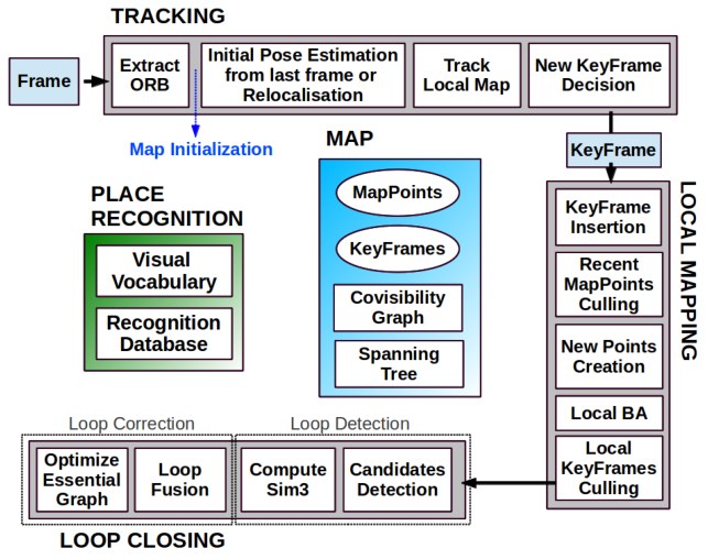
Fig. 1. ORB-SLAM system overview, showing all the steps performed by the tracking, local mapping and loop closing threads. The main components of the place recognition module and the map are also shown.
图 1. ORB-SLAM 系统概览,给出跟踪、局部建图和回环闭合线程所执行的全部步骤。位置识别模块和地图的主要组成部分也一并给出。
Our system, see an overview in Fig. 1, incorporates three threads that run in parallel: tracking, local mapping and loop closing. The tracking is in charge of localizing the camera with every frame and deciding when to insert a new keyframe. We perform first an initial feature matching with the previous frame and optimize the pose using motion-only BA. If the tracking is lost (e.g. due to occlusions or abrupt movements), the place recognition module is used to perform a global relocalization. Once there is an initial estimation of the camera pose and feature matchings, a local visible map is retrieved using the covisibility graph of keyframes that is maintained by the system, see Fig. 2(a) and Fig. 2(b). Then matches with the local map points are searched by reprojection, and camera pose is optimized again with all matches. Finally the tracking thread decides if a new keyframe is inserted. All the tracking steps are explained in detail in Section V. The novel procedure to create an initial map is presented in Section IV.
我们的系统,概览见图 1,包含三条并行运行的线程:跟踪、局部建图和回环闭合。跟踪负责用每一帧定位相机,并决定何时插入新的关键帧。我们先与上一帧做初始特征匹配,并用仅运动 BA 优化位姿。如果跟踪丢失(例如由于遮挡或突然运动),就用位置识别模块做全局重定位。一旦有了相机位姿和特征匹配的初始估计,就利用系统维护的关键帧共视图检索局部可见地图,见图 2(a) 和 图 2(b)。然后通过重投影搜索与局部地图点的匹配,并用全部匹配再次优化相机位姿。最后,跟踪线程决定是否插入新的关键帧。全部跟踪步骤在第 V 节详细说明。创建初始地图的新程序在第 IV 节给出。
The local mapping processes new keyframes and performs local BA to achieve an optimal reconstruction in the surroundings of the camera pose. New correspondences for unmatched ORB in the new keyframe are searched in connected keyframes in the covisibility graph to triangulate new points. Some time after creation, based on the information gathered during the tracking, an exigent point culling policy is applied in order to retain only high quality points. The local mapping is also in charge of culling redundant keyframes. We explain in detail all local mapping steps in Section VI.
局部建图处理新的关键帧,并做局部 BA,以在相机位姿周围得到最优重建。对新关键帧中尚未匹配的 ORB,在共视图中相连的关键帧里搜索新的对应,以三角化新的点。在创建一段时间之后,根据跟踪过程中收集的信息,施加严格的点裁减策略,以便只保留高质量的点。局部建图还负责裁减冗余关键帧。我们在第 VI 节详细说明全部局部建图步骤。
The loop closing searches for loops with every new keyframe. If a loop is detected, we compute a similarity transformation that informs about the drift accumulated in the loop. Then both sides of the loop are aligned and duplicated points are fused. Finally a pose graph optimization over similarity constraints [6] is performed to achieve global consistency. The main novelty is that we perform the optimization over the Essential Graph, a sparser subgraph of the covisibility graph which is explained in Section III-D. The loop detection and correction steps are explained in detail in Section VII.
回环闭合对每一个新关键帧搜索回环。如果检测到回环,我们就计算一个相似变换,以反映回环中累积的漂移。然后对齐回环的两侧,并融合重复的点。最后,在相似约束上做位姿图优化 [6],以实现全局一致性。主要新意在于,我们是在 Essential Graph 上做这一优化,它是共视图的一个更稀疏的子图,将在第 III-D 节说明。回环检测和校正步骤在第 VII 节详细说明。
We use the Levenberg-Marquardt algorithm implemented in g2o [37] to carry out all optimizations. In the Appendix we describe the error terms, cost functions, and variables involved in each optimization.
我们使用在 g2o [37] 中实现的 Levenberg-Marquardt 算法来进行全部优化。在附录中,我们描述了每一种优化所涉及的误差项、代价函数和变量。
C. Map Points, KeyFrames and their Selection
Each map point stores:
每个地图点 存储:
- Its 3D position in the world coordinate system.
- 它在世界坐标系中的三维位置 。
- The viewing direction , which is the mean unit vector of all its viewing directions (the rays that join the point with the optical center of the keyframes that observe it).
- 观测方向 ,它是该点所有观测方向的平均单位向量(连接该点与观测它的关键帧光心的射线)。
- A representative ORB descriptor , which is the associated ORB descriptor whose hamming distance is minimum with respect to all other associated descriptors in the keyframes in which the point is observed.
- 一个代表性的 ORB 描述子 ,它是在观测该点的关键帧中,与所有其他关联描述子的汉明距离最小的那个关联 ORB 描述子。
- The maximum and minimum distances at which the point can be observed, according to the scale invariance limits of the ORB features.
- 根据 ORB 特征的尺度不变范围,该点可被观测到的最大距离 和最小距离 。
Each keyframe stores:
每个关键帧 存储:
- The camera pose , which is a rigid body transformation that transforms points from the world to the camera coordinate system.
- 相机位姿 ,这是一个把点从世界坐标系变换到相机坐标系的刚体变换。
- The camera intrinsics, including focal length and principal point.
- 相机内参,包括焦距和主点。
- All the ORB features extracted in the frame, associated or not to a map point, whose coordinates are undistorted if a distortion model is provided.
- 该帧中提取的全部 ORB 特征,不论是否已关联到地图点;若提供了畸变模型,其坐标已去畸变。
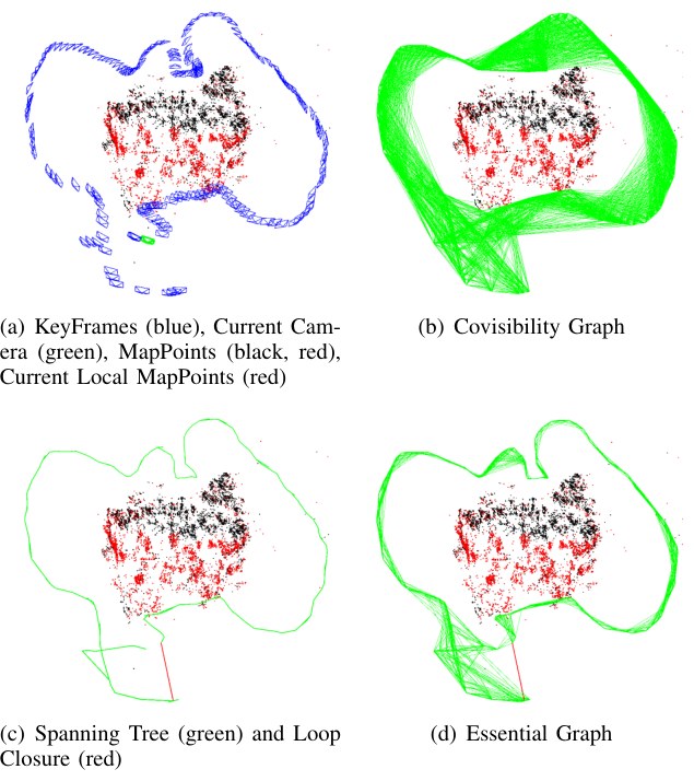
Fig. 2. Reconstruction and graphs in the sequence fr3_long_office_household from the TUM RGB-D Benchmark [38]. (a) KeyFrames (blue), Current Camera (green), MapPoints (black, red), Current Local MapPoints (red). (b) Covisibility Graph. (c) Spanning Tree (green) and Loop Closure (red). (d) Essential Graph.
图 2. TUM RGB-D 基准 [38] 中序列 fr3_long_office_household 的重建与图。(a) 关键帧(蓝色)、当前相机(绿色)、地图点(黑色、红色)、当前局部地图点(红色)。(b) 共视图。(c) 生成树(绿色)和回环闭合(红色)。(d) Essential Graph。
Map points and keyframes are created with a generous policy, while a later very exigent culling mechanism is in charge of detecting redundant keyframes and wrongly matched or not trackable map points. This permits a flexible map expansion during exploration, which boost tracking robustness under hard conditions (e.g. rotations, fast movements), while its size is bounded in continual revisits to the same environment, i.e. lifelong operation. Additionally our maps contain very few outliers compared with PTAM, at the expense of containing less points. Culling procedures of map points and keyframes are explained in Sections VI-B and VI-E respectively.
地图点和关键帧以较为慷慨的策略创建,而随后非常严格的裁减机制负责检测冗余关键帧,以及匹配错误或不可跟踪的地图点。这允许在探索过程中灵活地扩展地图,从而在困难条件(例如旋转、快速运动)下提高跟踪鲁棒性;而在不断回访同一环境时,其规模又保持有界,也就是可以长期运行。此外,与 PTAM 相比,我们的地图离群点很少,代价是包含的点更少。地图点和关键帧的裁减程序分别在第 VI-B 和 VI-E 节说明。
D. Covisibility Graph and Essential Graph
Covisibility information between keyframes is very useful in several tasks of our system, and is represented as an undirected weighted graph as in [7]. Each node is a keyframe and an edge between two keyframes exists if they share observations of the same map points (at least 15), being the weight of the edge the number of common map points.
关键帧之间的共视信息在我们系统的多项任务中非常有用,并像 [7] 中那样表示成无向加权图。每个节点是一个关键帧,若两个关键帧共享对同一批地图点的观测(至少 15 个),则它们之间存在一条边,边的权重 是共有地图点的数量。
In order to correct a loop we perform a pose graph optimization [6] that distributes the loop closing error along the graph. In order not to include all the edges provided by the covisibility graph, which can be very dense, we propose to build an Essential Graph that retains all the nodes (keyframes), but less edges, still preserving a strong network that yields accurate results. The system builds incrementally a spanning tree from the initial keyframe, which provides a connected subgraph of the covisibility graph with minimal number of edges. When a new keyframe is inserted, it is included in the tree linked to the keyframe which shares most point observations, and when a keyframe is erased by the culling policy, the system updates the links affected by that keyframe. The Essential Graph contains the spanning tree, the subset of edges from the covisibility graph with high covisibility (), and the loop closure edges, resulting in a strong network of cameras. Fig. 2 shows an example of a covisibility graph, spanning tree and associated essential graph. As shown in the experiments of Section VIII-E, when performing the pose graph optimization, the solution is so accurate that an additional full bundle adjustment optimization barely improves the solution. The efficiency of the essential graph and the influence of the is shown at the end of Section VIII-E.
为了校正回环,我们做一次位姿图优化 [6],把回环闭合误差沿图分配。为了不把共视图提供的全部边都包括进来——这些边可能非常密——我们提出构建 Essential Graph,它保留全部节点(关键帧),但边更少,同时仍保持一个能产生精确结果的牢固网络。系统从初始关键帧起增量地构建一棵生成树,它提供共视图中边数最少的连通子图。当插入新关键帧时,它被链到共享最多点观测的那个关键帧并加入树中;当关键帧被裁减策略删除时,系统更新受该关键帧影响的链接。Essential Graph 包含生成树、共视图中共视程度高()的那一部分边,以及回环闭合边,从而形成一个牢固的相机网络。图 2 给出了共视图、生成树和相应 Essential Graph 的一个例子。如第 VIII-E 节实验所示,在做完位姿图优化后,解已经足够精确,再做一次完整束调整几乎不再改进结果。Essential Graph 的效率以及 的影响,在第 VIII-E 节末给出。
E. Bags of Words Place Recognition
The system has embedded a bags of words place recognition module, based on DBoW2^{2} [5], to perform loop detection and relocalization. Visual words are just a discretization of the descriptor space, which is known as the visual vocabulary. The vocabulary is created offline with the ORB descriptors extracted from a large set of images. If the images are general enough, the same vocabulary can be used for different environments getting a good performance, as shown in our previous work [11]. The system builds incrementally a database that contains an invert index, which stores for each visual word in the vocabulary, in which keyframes it has been seen, so that querying the database can be done very efficiently. The database is also updated when a keyframe is deleted by the culling procedure.
系统内嵌了一个基于 DBoW2^{2} [5] 的词袋位置识别模块,用于回环检测和重定位。视觉词只是描述子空间的一种离散化,称为视觉词典。词典离线创建,使用从大批图像中提取的 ORB 描述子。如果这些图像足够一般,同一词典就可以用于不同环境并取得良好表现,如我们此前的工作 [11] 所示。系统增量地构建一个包含倒排索引的数据库,对词典中的每个视觉词存储它曾在哪些关键帧中出现,从而可以非常高效地查询数据库。当关键帧被裁减程序删除时,数据库也会更新。
Because there exists visual overlap between keyframes, when querying the database there will not exist a unique keyframe with a high score. The original DBoW2 took this overlapping into account, adding up the score of images that are close in time. This has the limitation of not including keyframes viewing the same place but inserted at a different time. Instead we group those keyframes that are connected in the covisibility graph. In addition our database returns all keyframe matches whose scores are higher than the 75% of the best score.
由于关键帧之间存在视觉重叠,查询数据库时不会存在唯一一个得分很高的关键帧。原来的 DBoW2 考虑了这种重叠,把时间上接近的图像得分加在一起。其局限是,不会把在不同时间插入、但看到同一地点的关键帧包括进来。我们改为把在共视图中相连的那些关键帧分组。此外,我们的数据库返回得分高于最高得分 75% 的全部关键帧匹配。
An additional benefit of the bags of words representation for feature matching was reported in [5]. When we want to compute the correspondences between two sets of ORB features, we can constraint the brute force matching only to those features that belong to the same node in the vocabulary tree at a certain level (we select the second out of six), speeding up the search. We use this trick when searching matches for triangulating new points, and at loop detection and relocalization. We also refine the correspondences with an orientation consistency test, see [11] for details, that discards outliers ensuring a coherent rotation for all correspondences.
词袋表示对特征匹配的另一项好处曾在 [5] 中报告。当我们要计算两组 ORB 特征之间的对应时,可以把暴力匹配限制在词汇树某一层上属于同一节点的那些特征(我们在六层中选择第二层),从而加快搜索。我们在为三角化新点搜索匹配,以及在回环检测和重定位时使用这一技巧。我们还用方向一致性检验来精炼对应,细节见 [11],它丢弃离群点,确保所有对应具有一致的旋转。
IV. AUTOMATIC MAP INITIALIZATION
The goal of the map initialization is to compute the relative pose between two frames to triangulate an initial set of map points. This method should be independent of the scene (planar or general) and should not require human intervention to select a good two-view configuration, i.e. a configuration with significant parallax. We propose to compute in parallel two geometrical models, a homography assuming a planar scene and a fundamental matrix assuming a non-planar scene. We then use a heuristic to select a model and try to recover the relative pose with a specific method for the selected model. Our method only initializes when it is certain that the two-view configuration is safe, detecting low-parallax cases and the well-known twofold planar ambiguity [27], avoiding to initialize a corrupted map. The steps of our algorithm are:
地图初始化的目标是计算两帧之间的相对位姿,以三角化一组初始地图点。该方法应与场景无关(平面或一般),并且不应需要人工介入来选择良好的两视图配置,也就是具有显著视差的配置。我们提出并行计算两个几何模型:假定平面场景的单应,以及假定非平面场景的基本矩阵。然后我们用一个启发式选择模型,并尝试用针对所选模型的特定方法恢复相对位姿。我们的方法只在确定两视图配置安全时才初始化,能够检测小视差情形以及众所周知的平面双重歧义 [27],避免初始化出被污染的地图。算法步骤如下:
- Find initial correspondences: Extract ORB features (only at the finest scale) in the current frame and search for matches in the reference frame . If not enough matches are found, reset the reference frame.
- 寻找初始对应:在当前帧 中提取 ORB 特征(只在最精细尺度上),并在参考帧 中搜索匹配 。如果找不到足够的匹配,就重置参考帧。
- Parallel computation of the two models: Compute in parallel threads a homography and a fundamental matrix :
- 并行计算两个模型:在并行线程中计算单应 和基本矩阵 :
with the normalized DLT and 8-point algorithms respectively as explained in [2] inside a RANSAC scheme. To make homogeneous the procedure for both models, the number of iterations is prefixed and the same for both models, along with the points to be used at each iteration, 8 for the fundamental matrix, and 4 of them for the homography. At each iteration we compute a score for each model ( for the homography, for the fundamental matrix):
分别用 [2] 中所述的归一化 DLT 和八点算法,并放在 RANSAC 方案中。为了使两个模型的流程一致,迭代次数预先固定且对两个模型相同,每一迭代所用的点也相同:基本矩阵用 8 个点,其中 4 个用于单应。在每一迭代中,我们为每个模型 ( 表示单应, 表示基本矩阵)计算一个得分 :
$$\begin{aligned}
S_M &= \sum_i \rho_M!\left(d_{\mathrm{cr}}^{2}(\mathbf{x}_c^{i}, \mathbf{x}r^{i}, M)\right) + \rho_M!\left(d{\mathrm{rc}}^{2}(\mathbf{x}_c^{i}, \mathbf{x}_r^{i}, M)\right), \
\rho_M(d^{2}) &=
\begin{cases}
\Gamma - d^{2} & \text{if } d^{2} < T_M \
0 & \text{if } d^{2} \ge T_M
\end{cases}
\tag{2}
\end{aligned}$$
where and are the symmetric transfer errors [2] from one frame to the other. is the outlier rejection threshold based on the test at 95% (, , assuming a standard deviation of 1 pixel in the measurement error). is defined equal to so that both models score equally for the same in their inlier region, again to make the process homogeneous. We keep the homography and fundamental matrix with highest score. If no model could be found (not enough inliers), we restart the process again from step 1.
其中 和 是从一帧到另一帧的对称转移误差 [2]。 是基于 95% 检验的离群点拒绝阈值(,,假定测量误差的标准差为 1 像素)。 被定义为等于 ,从而使两个模型在其内点区域内对同一 得分相同,同样是为了使流程一致。我们保留得分最高的单应和基本矩阵。如果找不到模型(内点不够),就从第 1 步重新开始。
- Model selection: If the scene is planar, nearly planar or there is low parallax, it can be explained by a homography. However a fundamental matrix can also be found, but the problem is not well constrained [2] and any attempt to recover the motion from the fundamental matrix would yield wrong results. We should select the homography as the reconstruction method will correctly initialize from a plane or it will detect the low parallax case and refuse the initialization. On the other hand a non-planar scene with enough parallax can only be explained by the fundamental matrix, but a homography can also be found explaining a subset of the matches if they lie on a plane or they have low parallax (they are far away). In this case we should select the fundamental matrix. We have found that a robust heuristic is to compute:
- 模型选择:如果场景是平面、接近平面,或视差很小,它可以用单应解释。不过也可以求出一个基本矩阵,但问题约束不足 [2],任何从基本矩阵恢复运动的尝试都会得到错误结果。我们应当选择单应,因为重建方法将正确地从平面初始化,或者会检测出小视差情形并拒绝初始化。另一方面,具有足够视差的非平面场景只能用基本矩阵解释,但也可以找到一个单应来解释匹配中的一个子集,如果它们落在一个平面上,或视差很小(它们很远)。在这种情形下我们应当选择基本矩阵。我们发现一个鲁棒的启发式是计算:
and select the homography if , which adequately captures the planar and low parallax cases. Otherwise, we select the fundamental matrix.
若 则选择单应,这充分捕捉了平面和小视差情形。否则,我们选择基本矩阵。
- Motion and Structure from Motion recovery: Once a model is selected we retrieve the motion hypotheses associated. In the case of the homography we retrieve 8 motion hypotheses using the method of Faugeras et. al [23]. The method proposes cheirality tests to select the valid solution. However these tests fail if there is low parallax as points easily go in front or back of the cameras, which could yield the selection of a wrong solution. We propose to directly triangulate the eight solutions, and check if there is one solution with most points seen with parallax, in front of both cameras and with low reprojection error. If there is not a clear winner solution, we do not initialize and continue from step 1. This technique to disambiguate the solutions makes our initialization robust under low parallax and the twofold ambiguity configuration, and could be considered the key of the robustness of our method.
- 运动与运动恢复结构:一旦选定模型,我们就取出相关的运动假设。在单应的情形中,我们用 Faugeras et. al [23] 的方法取出 8 个运动假设。该方法提出用手性检验来选择有效解。然而,如果视差很小,这些检验会失败,因为点很容易跑到相机前方或后方,从而可能选出错误的解。我们提出直接对这八个解做三角化,并检查是否存在一个解,其大多数点在有视差的情况下被看到、位于两个相机前方,并且重投影误差较低。如果没有明显的优胜解,我们就不初始化,并从第 1 步继续。这种消除解歧义的技术,使我们的初始化在小视差和双重歧义配置下保持鲁棒,可以被视为我们方法鲁棒性的关键。
In the case of the fundamental matrix, we convert it in an essential matrix using the calibration matrix :
在基本矩阵的情形中,我们用标定矩阵 把它转换成本质矩阵:
and then retrieve 4 motion hypotheses with the singular value decomposition method explained in [2]. We triangulate the four solutions and select the reconstruction as done for the homography.
然后用 [2] 中所述的奇异值分解方法取出 4 个运动假设。我们对这四个解做三角化,并像单应情形那样选择重建。
- Bundle adjustment: Finally we perform a full BA, see the Appendix for details, to refine the initial reconstruction.
- 束调整:最后我们做一次完整 BA,细节见附录,以精炼初始重建。
An example of a challenging initialization in the outdoor NewCollege robot sequence [39] is shown in Fig. 3. It can be seen how PTAM and LSD-SLAM have initialized all points in a plane, while our method has waited until there is enough parallax, initializing correctly from the fundamental matrix.
图 3 给出了户外 NewCollege 机器人序列 [39] 中一次具有挑战性的初始化例子。可以看到 PTAM 和 LSD-SLAM 把所有点都初始化在一个平面上,而我们的方法等到有足够视差之后,才正确地从基本矩阵初始化。
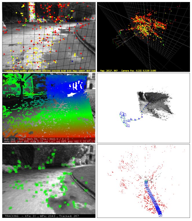
Fig. 3. Top: PTAM, middle LSD-SLAM, bottom: ORB-SLAM, some time after initialization in the NewCollege sequence [39]. PTAM and LSD-SLAM initialize a corrupted planar solution while our method has automatically initialized from the fundamental matrix when it has detected enough parallax. Depending on which keyframes are manually selected, PTAM is also able to initialize well.
图 3. 上:PTAM,中:LSD-SLAM,下:ORB-SLAM,在 NewCollege 序列 [39] 初始化后不久。PTAM 和 LSD-SLAM 初始化出一个被污染的平面解,而我们的方法在检测到足够视差后,已自动从基本矩阵初始化。取决于手工选择哪些关键帧,PTAM 也能够初始化得很好。
V. TRACKING
In this section we describe the steps of the tracking thread that are performed with every frame from the camera. The camera pose optimizations, mentioned in several steps, consist in motion-only BA, which is described in the Appendix.
本节描述跟踪线程对来自相机的每一帧所执行的步骤。若干步骤中提到的相机位姿优化,都是仅运动 BA,将在附录中说明。
A. ORB Extraction
We extract FAST corners at 8 scale levels with a scale factor of 1.2. For image resolutions from to pixels we found suitable to extract 1000 corners, for higher resolutions, as the in the KITTI dataset [40] we extract 2000 corners. In order to ensure an homogeneous distribution we divide each scale level in a grid, trying to extract at least 5 corners per cell. Then we detect corners in each cell, adapting the detector threshold if not enough corners are found. The amount of corners retained per cell is also adapted if some cells contains no corners (textureless or low contrast). The orientation and ORB descriptor are then computed on the retained FAST corners. The ORB descriptor is used in all feature matching, in contrast to the search by patch correlation in PTAM.
我们在 8 个尺度层级上提取 FAST 角点,尺度因子为 1.2。对 到 像素的图像分辨率,我们发现提取 1000 个角点比较合适;对更高分辨率,例如 KITTI 数据集 [40] 中的 ,我们提取 2000 个角点。为了确保分布均匀,我们把每个尺度层级划分成网格,试图在每个格子中至少提取 5 个角点。然后在每个格子中检测角点,如果找不到足够的角点,就调整检测器阈值。若某些格子不含角点(无纹理或对比度低),每个格子保留的角点数量也会调整。随后在保留的 FAST 角点上计算方向和 ORB 描述子。全部特征匹配都使用 ORB 描述子,这与 PTAM 中按块相关搜索形成对比。
B. Initial Pose Estimation from Previous Frame
If tracking was successful for last frame, we use a constant velocity motion model to predict the camera pose and perform a guided search of the map points observed in the last frame. If not enough matches were found (i.e. motion model is clearly violated), we use a wider search of the map points around their position in the last frame. The pose is then optimized with the found correspondences.
如果上一帧跟踪成功,我们就用匀速运动模型预测相机位姿,并对上一帧中观测到的地图点做引导搜索。如果找不到足够的匹配(也就是运动模型明显被违反),我们就在这些地图点于上一帧中的位置附近做更宽的搜索。随后用找到的对应优化位姿。
C. Initial Pose Estimation via Global Relocalization
If the tracking is lost, we convert the frame into bag of words and query the recognition database for keyframe candidates for global relocalization. We compute correspondences with ORB associated to map points in each keyframe, as explained in section III-E. We then perform alternatively RANSAC iterations for each keyframe and try to find a camera pose using the PnP algorithm [41]. If we find a camera pose with enough inliers, we optimize the pose and perform a guided search of more matches with the map points of the candidate keyframe. Finally the camera pose is again optimized, and if supported with enough inliers, tracking procedure continues.
如果跟踪丢失,我们把该帧转换成词袋,并向识别数据库查询用于全局重定位的关键帧候选。我们按第 III-E 节所述,计算与每个关键帧中关联到地图点的 ORB 的对应。然后我们对每个关键帧交替做 RANSAC 迭代,并尝试用 PnP 算法 [41] 找到相机位姿。如果我们找到一个具有足够内点的相机位姿,就优化该位姿,并与候选关键帧的地图点做引导搜索以找到更多匹配。最后再次优化相机位姿,若有足够内点支持,跟踪程序就继续进行。
D. Track Local Map
Once we have an estimation of the camera pose and an initial set of feature matches, we can project the map into the frame and search more map point correspondences. To bound the complexity in large maps, we only project a local map. This local map contains the set of keyframes , that share map points with the current frame, and a set with neighbors to the keyframes in the covisibility graph. The local map also has a reference keyframe which shares most map points with current frame. Now each map point seen in and is searched in the current frame as follows:
一旦有了相机位姿的估计和一组初始特征匹配,我们就可以把地图投影到该帧中,并搜索更多的地图点对应。为了在大型地图中限制复杂度,我们只投影局部地图。该局部地图包含与当前帧共享地图点的关键帧集合 ,以及在共视图中与 中关键帧相邻的集合 。局部地图还有一个参考关键帧 ,它与当前帧共享最多的地图点。现在,在 和 中看到的每个地图点按如下方式在当前帧中搜索:
- Compute the map point projection in the current frame. Discard if it lays out of the image bounds.
- 计算该地图点在当前帧中的投影 。如果它落在图像边界之外,就丢弃。
- Compute the angle between the current viewing ray and the map point mean viewing direction . Discard if .
- 计算当前观测射线 与该地图点平均观测方向 之间的夹角。如果 ,就丢弃。
- Compute the distance from map point to camera center. Discard if it is out of the scale invariance region of the map point .
- 计算地图点到相机中心的距离 。如果它超出该地图点的尺度不变区域 ,就丢弃。
- Compute the scale in the frame by the ratio .
- 用比值 计算该帧中的尺度。
- Compare the representative descriptor of the map point with the still unmatched ORB features in the frame, at the predicted scale, and near , and associate the map point with the best match.
- 在预测尺度上、在 附近,把该地图点的代表性描述子 与该帧中尚未匹配的 ORB 特征比较,并把该地图点与最佳匹配关联。
The camera pose is finally optimized with all the map points found in the frame.
最后用该帧中找到的全部地图点优化相机位姿。
E. New Keyframe Decision
The last step is to decide if the current frame is spawned as a new keyframe. As there is a mechanism in the local mapping to cull redundant keyframes, we will try to insert keyframes as fast as possible, because that makes the tracking more robust to challenging camera movements, typically rotations. To insert a new keyframe all the following conditions must be met:
最后一步是决定当前帧是否生成新的关键帧。由于局部建图中有裁减冗余关键帧的机制,我们将尽可能快地插入关键帧,因为这使跟踪对具有挑战性的相机运动(通常是旋转)更加鲁棒。要插入新的关键帧,必须满足以下全部条件:
- More than 20 frames must have passed from the last global relocalization.
- 距上次全局重定位必须已经过去 20 帧以上。
- Local mapping is idle, or more than 20 frames have passed from last keyframe insertion.
- 局部建图处于空闲,或者距上次插入关键帧已经过去 20 帧以上。
- Current frame tracks at least 50 points.
- 当前帧至少跟踪到 50 个点。
- Current frame tracks less than 90% points than .
- 当前帧跟踪到的点数少于 的 90%。
Instead of using a distance criterion to other keyframes as PTAM, we impose a minimum visual change (condition 4). Condition 1 ensures a good relocalization and condition 3 a good tracking. If a keyframe is inserted when the local mapping is busy (second part of condition 2), a signal is sent to stop local bundle adjustment, so that it can process as soon as possible the new keyframe.
我们不是像 PTAM 那样使用与其他关键帧的距离准则,而是施加一个最小视觉变化(条件 4)。条件 1 确保良好的重定位,条件 3 确保良好的跟踪。如果在局部建图正忙时插入关键帧(条件 2 的后半部分),就发送一个信号以停止局部束调整,从而使它能够尽快处理新的关键帧。
VI. LOCAL MAPPING
In this section we describe the steps performed by the local mapping with every new keyframe .
本节描述局部建图对每一个新关键帧 所执行的步骤。
A. KeyFrame Insertion
At first we update the covisibility graph, adding a new node for and updating the edges resulting from the shared map points with other keyframes. We then update the spanning tree linking with the keyframe with most points in common. We then compute the bags of words representation of the keyframe, that will help in the data association for triangulating new points.
首先我们更新共视图,为 加入一个新节点,并更新由与其他关键帧共享地图点而产生的边。然后我们更新生成树,把 链到共有点最多的那个关键帧。随后我们计算该关键帧的词袋表示,它将有助于为三角化新点做数据关联。
B. Recent Map Points Culling
Map points, in order to be retained in the map, must pass a restrictive test during the first three keyframes after creation, that ensures that they are trackable and not wrongly triangulated, i.e due to spurious data association. A point must fulfill these two conditions:
地图点要保留在地图中,必须在创建后的前三个关键帧期间通过一项严格检验,以确保它们可跟踪且没有被错误三角化,例如由于虚假的数据关联。一个点必须满足这两个条件:
- The tracking must find the point in more than the 25% of the frames in which it is predicted to be visible.
- 跟踪必须在该点被预测为可见的帧中,超过 25% 的帧里找到该点。
- If more than one keyframe has passed from map point creation, it must be observed from at least three keyframes.
- 如果自地图点创建以来已经过去一个以上关键帧,它必须至少被三个关键帧观测到。
Once a map point have passed this test, it can only be removed if at any time it is observed from less than three keyframes. This can happen when keyframes are culled and when local bundle adjustment discards outlier observations. This policy makes our map contain very few outliers.
一旦地图点通过了这一检验,就只有在任何时候被少于三个关键帧观测到时才会被删除。这可能发生在关键帧被裁减,以及局部束调整丢弃离群观测时。这一策略使我们的地图只含很少的离群点。
C. New Map Point Creation
New map points are created by triangulating ORB from connected keyframes in the covisibility graph. For each unmatched ORB in we search a match with other unmatched point in other keyframe. This matching is done as explained in Section III-E and discard those matches that do not fulfill the epipolar constraint. ORB pairs are triangulated, and to accept the new points, positive depth in both cameras, parallax, reprojection error and scale consistency are checked. Initially a map point is observed from two keyframes but it could be matched in others, so it is projected in the rest of connected keyframes, and correspondences are searched as detailed in section V-D.
新的地图点通过三角化共视图中相连关键帧 的 ORB 来创建。对 中每一个尚未匹配的 ORB,我们在其他关键帧中搜索与其他尚未匹配点的匹配。这一匹配按第 III-E 节所述进行,并丢弃不满足对极约束的那些匹配。对 ORB 对做三角化,为了接受新的点,要检查两相机中的正深度、视差、重投影误差和尺度一致性。最初一个地图点由两个关键帧观测,但它也可能在其他帧中被匹配,因此它被投影到其余相连关键帧中,并按第 V-D 节所述搜索对应。
D. Local Bundle Adjustment
The local BA optimizes the currently processed keyframe , all the keyframes connected to it in the covisibility graph , and all the map points seen by those keyframes. All other keyframes that see those points but are not connected to the currently processed keyframe are included in the optimization but remain fixed. Observations that are marked as outliers are discarded at the middle and at the end of the optimization. See the Appendix for more details about this optimization.
局部 BA 优化当前正在处理的关键帧 、在共视图中与它相连的全部关键帧 ,以及这些关键帧所看到的全部地图点。所有看到这些点、但与当前正在处理的关键帧不相连的其他关键帧,也被纳入优化,但保持固定。被标记为离群点的观测在优化的中途和结束时被丢弃。关于这一优化的更多细节见附录。
E. Local Keyframe Culling
In order to maintain a compact reconstruction, the local mapping tries to detect redundant keyframes and delete them. This is beneficial as bundle adjustment complexity grows with the number of keyframes, but also because it enables lifelong operation in the same environment as the number of keyframes will not grow unbounded, unless the visual content in the scene changes. We discard all the keyframes in whose 90% of the map points have been seen in at least other three keyframes in the same or finer scale. The scale condition ensures that map points maintain keyframes from which they are measured with most accuracy. This policy was inspired by the one proposed in the work of Tan et. al [24], where keyframes were discarded after a process of change detection.
为了保持紧凑的重建,局部建图试图检测冗余关键帧并删除它们。这是有益的,因为束调整的复杂度随关键帧数量增长,也因为它使系统能够在同一环境中长期运行:除非场景中的视觉内容发生变化,关键帧数量不会无限增长。我们丢弃 中所有这样的关键帧:其 90% 的地图点已在至少另外三个相同或更精细尺度的关键帧中被看到。尺度条件确保地图点保留那些对它们测量最精确的关键帧。这一策略受到 Tan et. al [24] 工作中所提方法的启发,他们是在一个变化检测过程之后丢弃关键帧。
VII. LOOP CLOSING
The loop closing thread takes , the last keyframe processed by the local mapping, and tries to detect and close loops. The steps are next described.
回环闭合线程取出局部建图处理的最后一个关键帧 ,并试图检测和闭合回环。步骤如下所述。
A. Loop Candidates Detection
At first we compute the similarity between the bag of words vector of and all its neighbors in the covisibility graph () and retain the lowest score . Then we query the recognition database and discard all those keyframes whose score is lower than . This is a similar operation to gain robustness as the normalizing score in DBoW2, which is computed from the previous image, but here we use covisibility information. In addition all those keyframes directly connected to are discarded from the results. To accept a loop candidate we must detect consecutively three loop candidates that are consistent (keyframes connected in the covisibility graph). There can be several loop candidates if there are several places with similar appearance to .
首先我们计算 的词袋向量与它在共视图中全部邻居()之间的相似度,并保留最低得分 。然后我们查询识别数据库,并丢弃得分低于 的所有关键帧。这是一种与 DBoW2 中从上一图像计算的归一化得分类似的、用于增强鲁棒性的操作,但这里我们使用共视信息。此外,所有与 直接相连的关键帧也从结果中丢弃。要接受一个回环候选,我们必须连续检测到三个一致的回环候选(在共视图中相连的关键帧)。如果有若干地方与 外观相似,就可以有多个回环候选。
B. Compute the Similarity Transformation
In monocular SLAM there are seven degrees of freedom in which the map can drift, three translations, three rotations and a scale factor [6]. Therefore to close a loop we need to compute a similarity transformation from the current keyframe to the loop keyframe that informs us about the error accumulated in the loop. The computation of this similarity will serve also as geometrical validation of the loop.
在单目 SLAM 中,地图可能在七个自由度上漂移:三个平移、三个旋转和一个尺度因子 [6]。因此,要闭合回环,我们需要计算从当前关键帧 到回环关键帧 的相似变换,以反映回环中累积的误差。计算这一相似变换也将作为回环的几何验证。
We first compute correspondences between ORB associated to map points in the current keyframe and the loop candidate keyframes, following the procedure explained in section III-E. At this point we have 3D to 3D correspondences for each loop candidate. We alternatively perform RANSAC iterations with each candidate, trying to find a similarity transformation using the method of Horn [42]. If we find a similarity with enough inliers, we optimize it (see the Appendix), and perform a guided search of more correspondences. We optimize it again and, if is supported by enough inliers, the loop with is accepted.
我们首先按第 III-E 节所述程序,计算当前关键帧中关联到地图点的 ORB 与回环候选关键帧之间的对应。此时,对每个回环候选我们都有三维到三维的对应。我们与每个候选交替做 RANSAC 迭代,试图用 Horn [42] 的方法找到相似变换。如果我们找到一个具有足够内点的相似变换 ,就优化它(见附录),并做引导搜索以找到更多对应。我们再次优化它,如果 有足够内点支持,就接受与 的回环。
C. Loop Fusion
The first step in the loop correction is to fuse duplicated map points and insert new edges in the covisibility graph that will attach the loop closure. At first the current keyframe pose is corrected with the similarity transformation and this correction is propagated to all the neighbors of , concatenating transformations, so that both sides of the loop get aligned. All map points seen by the loop keyframe and its neighbors are projected into and its neighbors and matches are searched in a narrow area around the projection, as done in section V-D. All those map points matched and those that were inliers in the computation of are fused. All keyframes involved in the fusion will update their edges in the covisibility graph effectively creating edges that attach the loop closure.
回环校正的第一步是融合重复的地图点,并在共视图中插入将连接回环闭合的新边。首先,当前关键帧位姿 用相似变换 校正,这一校正通过级联变换传播到 的所有邻居,从而使回环两侧对齐。回环关键帧及其邻居所看到的全部地图点被投影到 及其邻居中,并像第 V-D 节那样在投影周围的狭窄区域内搜索匹配。所有匹配到的地图点,以及在计算 时作为内点的那些点,都被融合。参与融合的全部关键帧将更新它们在共视图中的边,从而有效地创建连接回环闭合的边。
D. Essential Graph Optimization
To effectively close the loop, we perform a pose graph optimization over the Essential Graph, described in Section III-D, that distributes the loop closing error along the graph. The optimization is performed over similarity transformations to correct the scale drift [6]. The error terms and cost function are detailed in the Appendix. After the optimization each map point is transformed according to the correction of one of the keyframes that observes it.
为了有效闭合回环,我们在第 III-D 节所述的 Essential Graph 上做位姿图优化,把回环闭合误差沿图分配。优化在相似变换上进行,以校正尺度漂移 [6]。误差项和代价函数在附录中详述。优化之后,每个地图点根据观测它的某一个关键帧的校正进行变换。
VIII. EXPERIMENTS
We have performed an extensive experimental validation of our system in the large robot sequence of NewCollege [39], evaluating the general performance of the system, in 16 hand-held indoor sequences of the TUM RGB-D benchmark [38], evaluating the localization accuracy, relocalization and lifelong capabilities, and in 10 car outdoor sequences from the KITTI dataset [40], evaluating real-time large scale operation, localization accuracy and efficiency of the pose graph optimization.
我们在 NewCollege 的大型机器人序列 [39] 上对系统的总体性能做了充分实验验证;在 TUM RGB-D 基准 [38] 的 16 条手持室内序列上评估定位精度、重定位和长期运行能力;并在 KITTI 数据集 [40] 的 10 条车载户外序列上评估实时大规模运行、定位精度以及位姿图优化的效率。
Our system runs in real time and processes the images exactly at the frame rate they were acquired. We have carried out all experiments with an Intel Core i7-4700MQ (4 cores @ 2.40GHz) and 8Gb RAM. ORB-SLAM has three main threads, that run in parallel with other tasks from ROS and the operating system, which introduces some randomness in the results. For this reason, in some experiments, we report the median from several runs.
系统实时运行,并按图像采集时的原始帧率处理。全部实验在 Intel Core i7-4700MQ(4 核 @ 2.40GHz)和 8Gb 内存上完成。ORB-SLAM 有三条主线程,它们与 ROS 及操作系统中的其他任务并行,结果因此带有一定随机性。所以在部分实验中,我们报告多次运行的中位数。
A. System Performance in the NewCollege Dataset
The NewCollege dataset [39] contains a 2.2km sequence from a robot traversing a campus and adjacent parks. The sequence is recorded by a stereo camera at 20 fps and a resolution 512×382. It contains several loops and fast rotations that makes the sequence quite challenging for monocular vision. To the best of our knowledge there is no other monocular system in the literature able to process this whole sequence. For example Strasdat et al. [7], despite being able to close loops and work in large scale environments, only showed monocular results for a small part of this sequence.
NewCollege 数据集 [39] 包含一条 2.2 公里的序列,由机器人穿越校园及邻近公园时采集。序列由立体相机以 20 fps、分辨率 512×382 记录,其中有若干回环和快速旋转,对单目视觉相当有挑战。据我们所知,文献中还没有其他单目系统能够处理整条序列。例如 Strasdat 等人 [7] 虽然能够闭合回环并在大规模环境中工作,却只给出了该序列一小段上的单目结果。
As an example of our loop closing procedure we show in Fig. 4 the detection of a loop with the inliers that support the similarity transformation. Fig. 5 shows the reconstruction before and after the loop closure. In red it is shown the local map, which after the loop closure extends along both sides of the loop closure. The whole map after processing the full sequence at its real frame-rate is shown in Fig. 6. The big loop on the right does not perfectly align because it was traversed in opposite directions and the place recognizer was not able to find loop closures.
作为回环闭合流程的例子,图 4 给出一次回环检测,并画出支持该相似变换的内点对应。图 5 给出回环闭合前后的重建。红色表示局部地图,回环闭合之后它沿闭合处两侧延伸。以真实帧率处理完整序列后的整张地图见图 6。右侧的大回环没有完全对齐,因为该段是沿相反方向穿越的,位置识别器没能找到回环闭合。
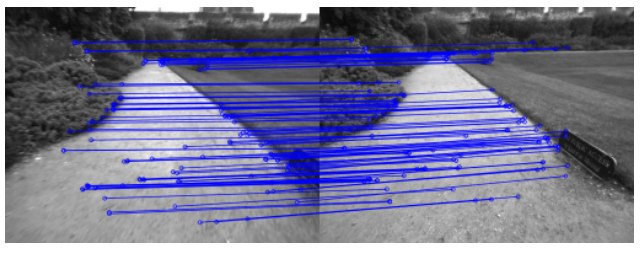
Fig. 4. Example of loop detected in the NewCollege sequence. We draw the inlier correspondences supporting the similarity transformation found.
图 4. NewCollege 序列中检测到的回环示例。我们画出支持所求得相似变换的内点对应。
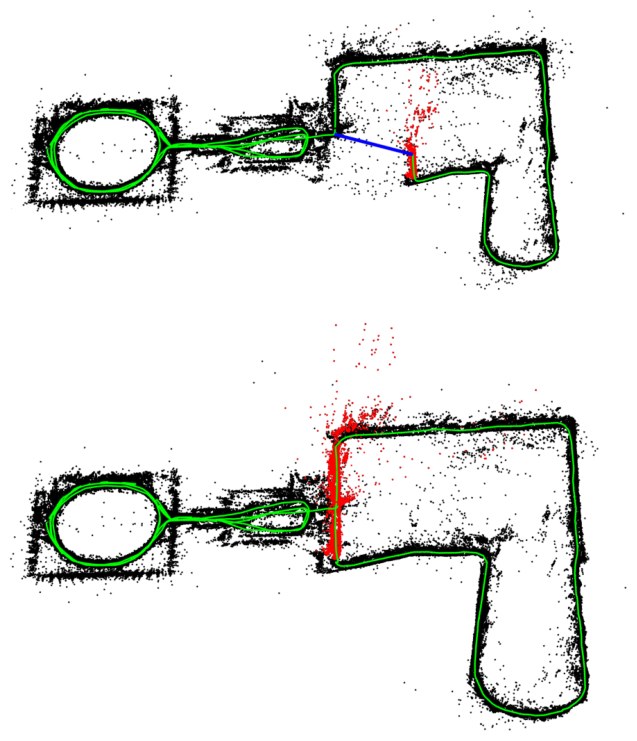
Fig. 5. Map before and after a loop closure in the NewCollege sequence. The loop closure match is drawn in blue, the trajectory in green, and the local map for the tracking at that moment in red. The local map is extended along both sides of the loop after it is closed.
图 5. NewCollege 序列中一次回环闭合前后的地图。回环闭合匹配画成蓝色,轨迹为绿色,当时跟踪所用的局部地图为红色。回环闭合后,局部地图沿回环两侧延伸。
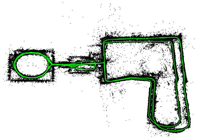
Fig. 6. ORB-SLAM reconstruction of the full sequence of NewCollege. The bigger loop on the right is traversed in opposite directions and not visual loop closures were found, therefore they do not perfectly align.
图 6. ORB-SLAM 对 NewCollege 完整序列的重建。右侧较大的回环沿相反方向穿越,没有找到视觉回环闭合,因此两侧并未完全对齐。
We have extracted statistics of the times spent by each thread in this experiment. Table I shows the results for the tracking and the local mapping. Tracking works at frame-rates around 25-30Hz, being the most demanding task to track the local map. If needed this time could be reduced limiting the number of keyframes that are included in the local map. In the local mapping thread the most demanding task is local bundle adjustment. The local BA time varies if the robot is exploring or in a well mapped area, because during exploration bundle adjustment is interrupted if tracking inserts a new keyframe, as explained in section V-E. In case of not needing new keyframes local bundle adjustment performs a generous number of prefixed iterations.
我们统计了本实验中各线程所耗时间。表 I 给出跟踪和局部建图的结果。跟踪工作在大约 25–30Hz 的帧率,其中最耗时的任务是跟踪局部地图。如有需要,可以通过限制纳入局部地图的关键帧数量来缩短这段时间。在局部建图线程中,最耗时的任务是局部束调整。局部 BA 的耗时会因机器人处于探索还是已建好地图的区域而变化:探索时,若跟踪插入了新关键帧,束调整会被打断,见第 V-E 节。若不需要新关键帧,局部束调整会执行预先设定的较多次迭代。
TABLE I
TRACKING AND MAPPING TIMES IN NEWCOLLEGE
| Thread | Operation | Median (ms) | Mean (ms) | Std (ms) |
|---|---|---|---|---|
| TRACKING | ORB extraction | 11.10 | 11.42 | 1.61 |
| TRACKING | Initial Pose Est. | 3.38 | 3.45 | 0.99 |
| TRACKING | Track Local Map | 14.84 | 16.01 | 9.98 |
| TRACKING | Total | 30.57 | 31.60 | 10.39 |
| LOCAL MAPPING | KeyFrame Insertion | 10.29 | 11.88 | 5.03 |
| LOCAL MAPPING | Map Point Culling | 0.10 | 3.18 | 6.70 |
| LOCAL MAPPING | Map Point Creation | 66.79 | 72.96 | 31.48 |
| LOCAL MAPPING | Local BA | 296.08 | 360.41 | 171.11 |
| LOCAL MAPPING | KeyFrame Culling | 8.07 | 15.79 | 18.98 |
| LOCAL MAPPING | Total | 383.59 | 464.27 | 217.89 |
表 I
NewCollege 中的跟踪与建图耗时
| 线程 | 操作 | 中位数 (ms) | 均值 (ms) | 标准差 (ms) |
|---|---|---|---|---|
| 跟踪 | ORB 提取 | 11.10 | 11.42 | 1.61 |
| 跟踪 | 初始位姿估计 | 3.38 | 3.45 | 0.99 |
| 跟踪 | 跟踪局部地图 | 14.84 | 16.01 | 9.98 |
| 跟踪 | 合计 | 30.57 | 31.60 | 10.39 |
| 局部建图 | 关键帧插入 | 10.29 | 11.88 | 5.03 |
| 局部建图 | 地图点剔除 | 0.10 | 3.18 | 6.70 |
| 局部建图 | 地图点创建 | 66.79 | 72.96 | 31.48 |
| 局部建图 | 局部 BA | 296.08 | 360.41 | 171.11 |
| 局部建图 | 关键帧剔除 | 8.07 | 15.79 | 18.98 |
| 局部建图 | 合计 | 383.59 | 464.27 | 217.89 |
Table II shows the results for each of the 6 loop closures found. It can be seen how the loop detection increases sublinearly with the number of keyframes. This is due to the efficient querying of the database that only compare the subset of images with words in common, which demonstrates the potential of bag of words for place recognition. Our Essential Graph includes edges around 5 times the number of keyframes, which is a quite sparse graph.
表 II 给出找到的 6 次回环闭合各自的结果。可以看到,回环检测耗时随关键帧数目亚线性增长。这是因为数据库查询很高效,只比较那些有共同单词的图像子集,也说明了词袋用于位置识别的潜力。我们的 Essential Graph 所含边数大约是关键帧数的 5 倍,是一张相当稀疏的图。
TABLE II
LOOP CLOSING TIMES IN NEWCOLLEGE
| Loop | KeyFrames | Essential Graph Edges | Loop Detection (ms): Candidates Detection | Loop Detection (ms): Similarity Transformation | Loop Correction (s): Fusion | Loop Correction (s): Essential Graph Optimization | Total (s) |
|---|---|---|---|---|---|---|---|
| 1 | 287 | 1347 | 4.71 | 20.77 | 0.20 | 0.26 | 0.51 |
| 2 | 1082 | 5950 | 4.14 | 17.98 | 0.39 | 1.06 | 1.52 |
| 3 | 1279 | 7128 | 9.82 | 31.29 | 0.95 | 1.26 | 2.27 |
| 4 | 2648 | 12547 | 12.37 | 30.36 | 0.97 | 2.30 | 3.33 |
| 5 | 3150 | 16033 | 14.71 | 41.28 | 1.73 | 2.80 | 4.60 |
| 6 | 4496 | 21797 | 13.52 | 48.68 | 0.97 | 3.62 | 4.69 |
表 II
NewCollege 中的回环闭合耗时
| 回环 | 关键帧 | Essential Graph 边数 | 回环检测 (ms):候选检测 | 回环检测 (ms):相似变换 | 回环校正 (s):融合 | 回环校正 (s):Essential Graph 优化 | 总计 (s) |
|---|---|---|---|---|---|---|---|
| 1 | 287 | 1347 | 4.71 | 20.77 | 0.20 | 0.26 | 0.51 |
| 2 | 1082 | 5950 | 4.14 | 17.98 | 0.39 | 1.06 | 1.52 |
| 3 | 1279 | 7128 | 9.82 | 31.29 | 0.95 | 1.26 | 2.27 |
| 4 | 2648 | 12547 | 12.37 | 30.36 | 0.97 | 2.30 | 3.33 |
| 5 | 3150 | 16033 | 14.71 | 41.28 | 1.73 | 2.80 | 4.60 |
| 6 | 4496 | 21797 | 13.52 | 48.68 | 0.97 | 3.62 | 4.69 |
B. Localization Accuracy in the TUM RGB-D Benchmark
The TUM RGB-D benchmark [38] is an excellent dataset to evaluate the accuracy of camera localization as it provides several sequences with accurate ground truth obtained with an external motion capture system. We have discarded all those sequences that we consider that are not suitable for pure monocular SLAM systems, as they contain strong rotations, no texture or no motion.
TUM RGB-D 基准 [38] 很适合评估相机定位精度,因为它提供若干带有外部运动捕捉系统所得精确真值的序列。我们剔除了所有认为不适合纯单目 SLAM 系统的序列,这些序列含有剧烈旋转、没有纹理或没有运动。
For comparison we have also executed the novel, direct, semi-dense LSD-SLAM [10] and PTAM [4] in the benchmark. We compare also with the trajectories generated by RGBD-SLAM [43] which are provided for some of the sequences in the benchmark website. In order to compare ORB-SLAM, LSD-SLAM and PTAM with the ground truth, we align the keyframe trajectories using a similarity transformation, as scale is unknown, and measure the absolute trajectory error (ATE) [38]. In the case of RGBD-SLAM we align the trajectories with a rigid body transformation, but also a similarity to check if the scale was well recovered. LSD-SLAM initializes from random depth values and takes time to converge, therefore we have discarded the first 10 keyframes when comparing with the ground truth. For PTAM we manually selected two frames from which we get a good initialization. Table III shows the median results over 5 executions in each of the 16 sequences selected.
为了比较,我们还在该基准上运行了较新的、直接法半稠密 LSD-SLAM [10] 以及 PTAM [4]。我们也与 RGBD-SLAM [43] 生成的轨迹比较,这些轨迹由基准网站为部分序列提供。为了把 ORB-SLAM、LSD-SLAM 和 PTAM 与真值比较,我们用相似变换对齐关键帧轨迹(因为尺度未知),并测量绝对轨迹误差(ATE)[38]。对 RGBD-SLAM,我们用刚体变换对齐轨迹,同时也用相似变换,以检查尺度是否恢复得当。LSD-SLAM 从随机深度值初始化,需要一段时间才能收敛,因此与真值比较时我们丢弃了前 10 个关键帧。对 PTAM,我们手工挑选了能够得到良好初始化的两帧。表 III 给出在所选 16 条序列上各运行 5 次的中位结果。
TABLE III
KEYFRAME LOCALIZATION ERROR COMPARISON IN THE TUM RGB-D BENCHMARK [38]
Absolute KeyFrame Trajectory RMSE (cm)
| Sequence | ORB-SLAM | PTAM | LSD-SLAM | RGBD-SLAM |
|---|---|---|---|---|
| fr1 xyz | 0.90 | 1.15 | 9.00 | 1.34 (1.34) |
| fr2 xyz | 0.30 | 0.20 | 2.15 | 2.61 (1.42) |
| fr1 floor | 2.99 | X | 38.07 | 3.51 (3.51) |
| fr1 desk | 1.69 | X | 10.65 | 2.58 (2.52) |
| fr2 360 kidnap | 3.81 | 2.63 | X | 393.3 (100.5) |
| fr2 desk | 0.88 | X | 4.57 | 9.50 (3.94) |
| fr3 long office | 3.45 | X | 38.53 | — |
| fr3 nstr tex far | ambiguity detected | 4.92 / 34.74 | 18.31 | — |
| fr3 nstr tex near | 1.39 | 2.74 | 7.54 | — |
| fr3 str tex far | 0.77 | 0.93 | 7.95 | — |
| fr3 str tex near | 1.58 | 1.04 | X | — |
| fr2 desk person | 0.63 | X | 31.73 | 6.97 (2.00) |
| fr3 sit xyz | 0.79 | 0.83 | 7.73 | — |
| fr3 sit halfsph | 1.34 | X | 5.87 | — |
| fr3 walk xyz | 1.24 | X | 12.44 | — |
| fr3 walk halfsph | 1.74 | X | X | — |
Results for ORB-SLAM, PTAM and LSD-SLAM are the median over 5 executions in each sequence. The trajectories have been aligned with 7DoF with the ground truth. Trajectories for RGBD-SLAM are taken from the benchmark website, only available for fr1 and fr2 sequences, and have been aligned with 6DoF and 7DoF (results between brackets). X means that the tracking is lost at some point and a significant portion of the sequence is not processed by the system.
表 III
TUM RGB-D 基准 [38] 上的关键帧定位误差比较
绝对关键帧轨迹 RMSE(厘米)
| 序列 | ORB-SLAM | PTAM | LSD-SLAM | RGBD-SLAM |
|---|---|---|---|---|
| fr1 xyz | 0.90 | 1.15 | 9.00 | 1.34 (1.34) |
| fr2 xyz | 0.30 | 0.20 | 2.15 | 2.61 (1.42) |
| fr1 floor | 2.99 | X | 38.07 | 3.51 (3.51) |
| fr1 desk | 1.69 | X | 10.65 | 2.58 (2.52) |
| fr2 360 kidnap | 3.81 | 2.63 | X | 393.3 (100.5) |
| fr2 desk | 0.88 | X | 4.57 | 9.50 (3.94) |
| fr3 long office | 3.45 | X | 38.53 | — |
| fr3 nstr tex far | 检测到二义性 | 4.92 / 34.74 | 18.31 | — |
| fr3 nstr tex near | 1.39 | 2.74 | 7.54 | — |
| fr3 str tex far | 0.77 | 0.93 | 7.95 | — |
| fr3 str tex near | 1.58 | 1.04 | X | — |
| fr2 desk person | 0.63 | X | 31.73 | 6.97 (2.00) |
| fr3 sit xyz | 0.79 | 0.83 | 7.73 | — |
| fr3 sit halfsph | 1.34 | X | 5.87 | — |
| fr3 walk xyz | 1.24 | X | 12.44 | — |
| fr3 walk halfsph | 1.74 | X | X | — |
ORB-SLAM、PTAM 和 LSD-SLAM 的结果是每条序列上 5 次运行的中位数。轨迹已用 7 自由度与真值对齐。RGBD-SLAM 的轨迹取自基准网站,仅有 fr1 和 fr2 序列,并分别用 6 自由度和 7 自由度对齐(括号内为后者)。X 表示跟踪在某处丢失,系统未能处理该序列的相当一部分。
It can be seen that ORB-SLAM is able to process all the sequences, except for fr3 nostructure texture far (fr3 nstr tex far). This is a planar scene that because of the camera trajectory with respect to the plane has two possible interpretations, i.e. the twofold ambiguity described in [27]. Our initialization method detects the ambiguity and for safety refuses to initialize. PTAM initializes selecting sometimes the true solution and others the corrupted one, in which case the error is unacceptable. We have not noticed two different reconstructions from LSD-SLAM but the error in this sequence is very high. In the rest of the sequences, PTAM and LSD-SLAM exhibit less robustness than our method, loosing track in eight and three sequences respectively.
可以看到,除了 fr3 nostructure texture far(fr3 nstr tex far)之外,ORB-SLAM 能够处理全部序列。这是一个平面场景,由于相机相对该平面的运动轨迹,存在两种可能的解释,也就是 [27] 所描述的双重二义性。我们的初始化方法检测到这一二义性,出于安全考虑拒绝初始化。PTAM 有时会选到正确解,有时会选到错误解,后一种情形下误差不可接受。我们没有在 LSD-SLAM 上看到两种不同的重建,但该序列上的误差非常高。在其余序列中,PTAM 和 LSD-SLAM 的鲁棒性不如我们的方法,分别在 8 条和 3 条序列上跟丢。
In terms of accuracy ORB-SLAM and PTAM are similar in open trajectories, while ORB-SLAM achieves higher accuracy when detecting large loops as in the sequence fr3 nostructure texture near withloop (fr3 nstr tex near). The most surprising results is that both PTAM and ORB-SLAM are clearly more accurate than LSD-SLAM and RGBD-SLAM. One of the possible causes can be that they reduce the map optimization to a pose-graph optimization were sensor measurements are discarded, while we perform bundle adjustment and jointly optimize cameras and map over sensor measurements, which is the gold standard algorithm to solve structure from motion [2]. We further discuss this result in Section IX-B. Another interesting result is that LSD-SLAM seems to be less robust to dynamic objects than our system as seen in fr2 desk with person and fr3 walking xyz.
就精度而言,ORB-SLAM 和 PTAM 在开放轨迹上相近,而在能够检测到大回环的序列上,例如 fr3 nostructure texture near withloop(fr3 nstr tex near),ORB-SLAM 精度更高。最令人意外的结果是,PTAM 和 ORB-SLAM 都明显比 LSD-SLAM 和 RGBD-SLAM 更准确。一个可能的原因是,后两者把地图优化简化成位姿图优化,传感器测量被丢弃;而我们做束调整,在传感器测量上联合优化相机和地图,这是求解运动恢复结构的金标准算法 [2]。我们将在第 IX-B 节进一步讨论这一结果。另一个有意思的结果是,LSD-SLAM 对动态物体的鲁棒性似乎不如我们的系统,这在 fr2 desk with person 和 fr3 walking xyz 中可以看出。
We have noticed that RGBD-SLAM has a bias in the scale in fr2 sequences, as aligning the trajectories with 7 DoF significantly reduces the error. Finally it should be noted that Engel et al. [10] reported that PTAM has less accuracy than LSD-SLAM in fr2 xyz with an RMSE of 24.28cm. However, the paper does not give enough details on how those results were obtained, and we have been unable to reproduce them.
我们注意到 RGBD-SLAM 在 fr2 序列上存在尺度偏差,因为用 7 自由度对齐轨迹会显著降低误差。最后应当指出,Engel 等人 [10] 曾报告 PTAM 在 fr2 xyz 上精度不如 LSD-SLAM,RMSE 为 24.28 厘米。不过该论文没有充分说明这些结果是如何得到的,我们也未能复现。
C. Relocalization in the TUM RGB-D Benchmark
We perform two relocalization experiments in the TUM RGB-D benchmark. In the first experiment we build a map with the first 30 seconds of the sequence fr2 xyz and perform global relocalization with every successive frame and evaluate the accuracy of the recovered poses. We perform the same experiment with PTAM for comparison. Fig. 7 shows the keyframes used to create the initial map, the poses of the relocalized frames and the ground truth for those frames. It can be seen that PTAM is only able to relocalize frames which are near to the keyframes due to the little invariance of its relocalization method. Table IV shows the recall and the error with respect to the ground truth. ORB-SLAM accurately relocalizes more than the double of frames than PTAM. In the second experiment we create an initial map with sequence fr3 sitting xyz and try to relocalize all frames from fr3 walking xyz. This is a challenging experiment as there are big occlusions due to people moving in the scene. Here PTAM finds no relocalizations while our system relocalizes 78% of the frames, as can be seen in Table IV. Fig. 8 shows some examples of challenging relocalizations performed by our system in these experiments.
我们在 TUM RGB-D 基准上做了两组重定位实验。第一组实验中,我们用序列 fr2 xyz 的前 30 秒建立地图,再对随后的每一帧做全局重定位,并评估恢复位姿的精度。为了比较,我们对 PTAM 做了同样的实验。图 7 给出用于建立初始地图的关键帧、重定位成功帧的位姿,以及这些帧的真值。可以看到,由于 PTAM 的重定位方法不变性较弱,它只能重定位靠近关键帧的那些帧。表 IV 给出相对于真值的召回和误差。ORB-SLAM 准确重定位的帧数是 PTAM 的两倍以上。第二组实验中,我们用序列 fr3 sitting xyz 建立初始地图,再尝试重定位 fr3 walking xyz 的全部帧。这是一个有挑战的实验,因为场景中有人走动,存在大面积遮挡。此时 PTAM 一次重定位都没有找到,而我们的系统重定位了 78% 的帧,见表 IV。图 8 给出这些实验中我们的系统所完成的若干有挑战的重定位例子。
TABLE IV
RESULTS FOR THE RELOCALIZATION EXPERIMENTS
| System | Initial Map KFs | Initial Map RMSE (cm) | Relocalization Recall (%) | Relocalization RMSE (cm) | Max. Error (cm) |
|---|---|---|---|---|---|
| fr2 xyz. 2769 frames to relocalize | |||||
| PTAM | 37 | 0.19 | 34.9 | 0.26 | 1.52 |
| ORB-SLAM | 24 | 0.19 | 78.4 | 0.38 | 1.67 |
| fr3 walking xyz. 859 frames to relocalize | |||||
| PTAM | 34 | 0.83 | 0.0 | — | — |
| ORB-SLAM | 31 | 0.82 | 77.9 | 1.32 | 4.95 |
表 IV
重定位实验结果
| 系统 | 初始地图关键帧数 | 初始地图 RMSE(厘米) | 重定位召回(%) | 重定位 RMSE(厘米) | 最大误差(厘米) |
|---|---|---|---|---|---|
| fr2 xyz。待重定位 2769 帧 | |||||
| PTAM | 37 | 0.19 | 34.9 | 0.26 | 1.52 |
| ORB-SLAM | 24 | 0.19 | 78.4 | 0.38 | 1.67 |
| fr3 walking xyz。待重定位 859 帧 | |||||
| PTAM | 34 | 0.83 | 0.0 | — | — |
| ORB-SLAM | 31 | 0.82 | 77.9 | 1.32 | 4.95 |
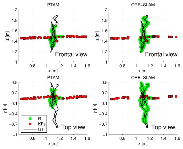
Fig. 7. Relocalization experiment in fr2 xyz. Map is initially created during the first 30 seconds of the sequence (KFs). The goal is to relocalize subsequent frames. Successful relocalizations (R) of our system and PTAM are shown. The ground truth (GT) is only shown for the frames to relocalize.
图 7. fr2 xyz 上的重定位实验。地图先用该序列前 30 秒建立(KFs)。目标是重定位随后的帧。图中给出我们的系统和 PTAM 的成功重定位(R)。真值(GT)只对需要重定位的那些帧画出。
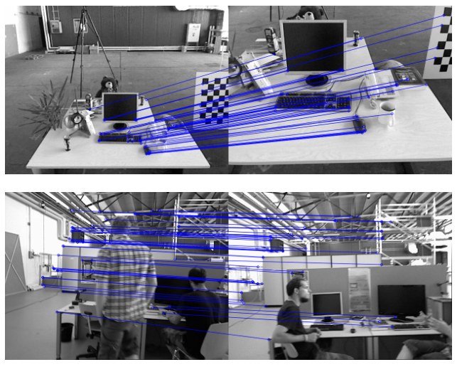
Fig. 8. Example of challenging relocalizations (severe scale change, dynamic objects) that our system successfully found in the relocalization experiments.
图 8. 重定位实验中我们的系统成功找到的有挑战的重定位例子(剧烈尺度变化、动态物体)。
D. Lifelong Experiment in the TUM RGB-D Benchmark
Previous relocalization experiments have shown that our system is able to localize in a map from very different viewpoints and robustly under moderate dynamic changes. This property in conjunction with our keyframe culling procedure allows to operate lifelong in the same environment under different viewpoints and some dynamic changes.
前面的重定位实验表明,我们的系统能够从差别很大的视角在已有地图中定位,并在中等程度的动态变化下保持稳健。这一性质再配合我们的关键帧剔除流程,使得系统可以在同一环境中、在不同视角和一定动态变化下长期运行。
In the case of a completely static scenario our system is able to maintain the number of keyframes bounded even if the camera is looking at the scene from different viewpoints. We demonstrate it in a custom sequence were the camera is looking at the same desk during 93 seconds but performing a trajectory so that the viewpoint is always changing. We compare the evolution of the number of keyframes in our map and those generated by PTAM in Fig. 9. It can be seen how PTAM is always inserting keyframes, while our mechanism to prune redundant keyframes makes its number to saturate.
在完全静态的场景中,即使相机从不同视角观察同一场景,我们的系统也能把关键帧数量维持在有界范围。我们在一条自制序列上展示这一点:相机在 93 秒内一直看同一张桌子,但轨迹使视角不断变化。我们在图 9 中比较了我们的地图与 PTAM 所生成关键帧数量的变化。可以看到,PTAM 一直在插入关键帧,而我们剔除冗余关键帧的机制使关键帧数目趋于饱和。
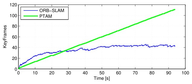
Fig. 9. Lifelong experiment in a static environment where the camera is always looking at the same place from different viewpoints. PTAM is always inserting keyframes, while ORB-SLAM is able to prune redundant keyframes and maintains a bounded-size map.
图 9. 静态环境中的长期运行实验:相机始终从不同视角看同一个地方。PTAM 一直在插入关键帧,而 ORB-SLAM 能够剔除冗余关键帧,把地图规模维持在有界范围。
While the lifelong operation in a static scenario should be a requirement of any SLAM system, more interesting is the case where dynamic changes occur. We analyze the behavior of our system in such scenario by running consecutively the dynamic sequences from fr3: sitting xyz, sitting halfsphere, sitting rpy, walking xyz, walking halfspehere and walking rpy. All the sequences focus the camera to the same desk but perform different trajectories, while people are moving and change some objects like chairs. Fig. 10(a) shows the evolution of the total number of keyframes in the map, and Fig. 10(b) shows for each keyframe its frame of creation and destruction, showing how long the keyframes have survived in the map. It can be seen that during the first two sequences the map size grows as all the views of the scene are being seen for the first time. In Fig. 10(b) we can see that several keyframes created during these two first sequences are maintained in the map during the whole experiment. During the sequences sitting rpy and walking xyz the map does not grow, because the map created so far explains well the scene. In contrast, during the last two sequences, more keyframes are inserted showing that there are some novelties in the scene that were not yet represented, due probably to dynamic changes.
静态场景下的长期运行应当是任何 SLAM 系统的基本要求,更有意思的是出现动态变化的情形。我们把 fr3 中的动态序列连续跑一遍,来分析系统在这种场景下的行为:sitting xyz、sitting halfsphere、sitting rpy、walking xyz、walking halfspehere 和 walking rpy。这些序列都把相机对准同一张桌子,但轨迹不同,同时有人走动,并改动椅子一类物体。图 10(a) 给出地图中关键帧总数的变化,图 10(b) 给出每个关键帧的创建帧与销毁帧,从而看出关键帧在地图中存活了多久。可以看到,前两条序列中地图规模在增长,因为场景的各个视角都是第一次看到。从图 10(b) 可以看出,前两条序列中创建的若干关键帧在整个实验期间都留在地图里。在 sitting rpy 和 walking xyz 期间,地图不再增长,因为至此建成的地图已经能够很好地解释该场景。相反,在最后两条序列中又插入了更多关键帧,说明场景中还有尚未被表示的新内容,这很可能来自动态变化。
Finally Fig. 10(c) shows a histogram of the keyframes according to the time they have survived with respect to the remaining time of the sequence from its moment of creation. It can be seen that most of the keyframes are destroyed by the culling procedure soon after creation, and only a small subset survive until the end of the experiment. On one hand, this shows that our system has a generous keyframe spawning policy, which is very useful when performing abrupt motions in exploration. On the other hand the system is eventually able to select a small representative subset of those keyframes.
最后,图 10(c) 按关键帧自创建时刻起、相对于序列剩余时间的存活比例给出直方图。可以看到,大多数关键帧在创建后不久就被剔除流程销毁,只有一小部分存活到实验结束。一方面,这说明我们的系统在生成关键帧时比较慷慨,这在探索中出现剧烈运动时很有用。另一方面,系统最终能够从这些关键帧中选出一个较小的代表性子集。
In these lifelong experiments we have shown that our map grows with the content of the scene but not with the time, and that is able to store the dynamic changes of the scene which could be useful to perform some scene understanding by accumulating experience in an environment.
在这些长期运行实验中,我们表明地图随场景内容增长,而不随时间增长,并且能够保存场景的动态变化;这或许有助于通过在同一环境中积累经验来做某种场景理解。
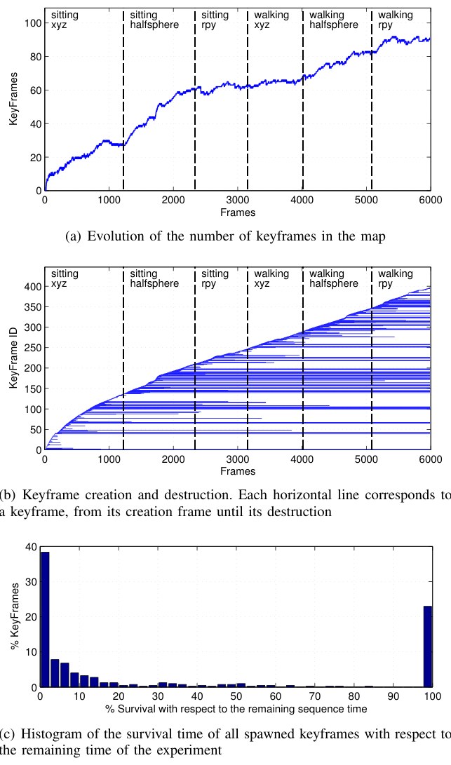
Fig. 10. Lifelong experiment in a dynamic environment from the TUM RGB-D Benchmark. (a) Evolution of the number of keyframes in the map. (b) Keyframe creation and destruction. Each horizontal line corresponds to a keyframe, from its creation frame until its destruction. (c) Histogram of the survival time of all spawned keyframes with respect to the remaining time of the experiment.
图 10. TUM RGB-D 基准中动态环境下的长期运行实验。(a) 地图中关键帧数目的变化。(b) 关键帧的创建与销毁。每条横线对应一个关键帧,从其创建帧直到销毁。(c) 全部生成关键帧的存活时间直方图,存活时间相对于实验剩余时间计算。
E. Large Scale and Large Loop Closing in the KITTI Dataset
The odometry benchmark from the KITTI dataset [40] contains 11 sequences from a car driven around a residential area with accurate ground truth from GPS and a Velodyne laser scanner. This is a very challenging dataset for monocular vision due to fast rotations, areas with lot of foliage, which make more difficult data association, and relatively high car speed, being the sequences recorded at 10 fps. We play the sequences at the real frame-rate they were recorded and ORB-SLAM is able to process all the sequences by the exception of sequence 01 which is a highway with few trackable close objects. Sequences 00, 02, 05, 06, 07, 09 contain loops that were correctly detected and closed by our system. Sequence 09 contains a loop that can be detected only in a few frames at the end of the sequence, and our system not always detects it (the results provided are for the executions in which it was detected).
KITTI 数据集 [40] 的里程计基准包含 11 条序列,由汽车在居住区行驶时采集,并带有 GPS 和 Velodyne 激光扫描仪提供的精确真值。这对单目视觉很有挑战:有快速旋转,有大量树叶的区域使数据关联更困难,车速也相对较快,序列以 10 fps 记录。我们按录制时的真实帧率播放这些序列,ORB-SLAM 能够处理除序列 01 以外的全部序列;序列 01 是高速公路,近处可跟踪的物体很少。序列 00、02、05、06、07、09 含有回环,都被我们的系统正确检测并闭合。序列 09 中的回环只能在序列末尾的少数几帧里被检测到,我们的系统并非每次都能检测到(所给结果对应检测到该回环的那些次运行)。
Qualitative comparisons of our trajectories and the ground truth are shown in Fig. 11 and Fig. 12. As in the TUM RGB-D benchmark we have aligned the keyframe trajectories of our system and the ground truth with a similarity transformation. We can compare qualitatively our results from Fig. 11 and Fig. 12 with the results provided for sequences 00, 05, 06, 07 and 08 by the recent monocular SLAM approach of Lim et. al [25] in their figure 10. ORB-SLAM produces clearly more accurate trajectories for all those sequences by the exception of sequence 08 in which they seem to suffer less drift.
我们的轨迹与真值的定性比较见图 11 和图 12。与 TUM RGB-D 基准中一样,我们用相似变换对齐系统的关键帧轨迹和真值。可以把图 11 和图 12 中的结果,与 Lim 等人 [25] 近期的单目 SLAM 方法在其图 10 中为序列 00、05、06、07 和 08 给出的结果做定性比较。除序列 08 上他们的漂移似乎更小之外,ORB-SLAM 在这些序列上都给出明显更准确的轨迹。
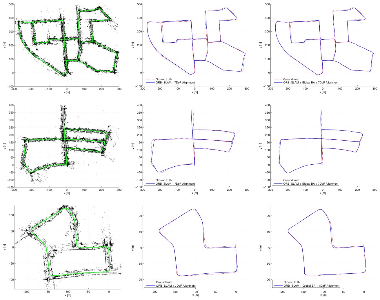
Fig. 11. Sequences 00, 05 and 07 from the odometry benchmark of the KITTI dataset. Left: points and keyframe trajectory. Center: trajectory and ground truth. Right: trajectory after 20 iterations of full BA. The output of our system is quite accurate, while it can be slightly improved with some iterations of BA.
图 11. KITTI 数据集里程计基准中的序列 00、05 和 07。左:点与关键帧轨迹。中:轨迹与真值。右:完整 BA 迭代 20 次后的轨迹。系统输出已经相当准确,再用若干次 BA 迭代还能略有改进。
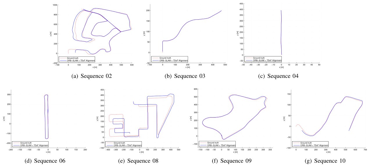
Fig. 12. ORB-SLAM keyframe trajectories in sequences 02, 03, 04 ,06, 08, 09 and 10 from the odometry benchmark of the KITTI dataset. Sequence 08 does not contains loops and drift (especially scale) is not corrected.
图 12. ORB-SLAM 在 KITTI 数据集里程计基准序列 02、03、04、06、08、09 和 10 上的关键帧轨迹。序列 08 不含回环,漂移(尤其是尺度)没有被校正。
Table V shows the median RMSE error of the keyframe trajectory over five executions in each sequence. We also provide the dimensions of the maps to put in context the errors. The trajectory error typically around the 1% of its dimensions, sometimes less as in sequence 03 with an error of the 0.3% or higher as in sequence 08 with the 5%. In sequence 08 there are no loops and drift cannot be corrected, which makes clear the need of loop closures to achieve accurate reconstructions.
表 V 给出每条序列上五次运行的关键帧轨迹中位 RMSE。我们还给出地图的尺寸,以便把误差放在相应尺度下来看。轨迹误差通常大约是其尺寸的 1%,有时更低,如序列 03 的误差为 0.3%,有时更高,如序列 08 的 5%。序列 08 没有回环,漂移无法校正,这清楚地说明要得到准确重建就需要回环闭合。
TABLE V
RESULTS OF OUR SYSTEM IN THE KITTI DATASET.
| Sequence | Dimension (m×m) | ORB-SLAM: KFs | ORB-SLAM: RMSE (m) | + Global BA (20 its.): RMSE (m) | + Global BA (20 its.): Time BA (s) |
|---|---|---|---|---|---|
| KITTI 00 | 564 × 496 | 1391 | 6.68 | 5.33 | 24.83 |
| KITTI 01 | 1157 × 1827 | X | X | X | X |
| KITTI 02 | 599 × 946 | 1801 | 21.75 | 21.28 | 30.07 |
| KITTI 03 | 471 × 199 | 250 | 1.59 | 1.51 | 4.88 |
| KITTI 04 | 0.5 × 394 | 108 | 1.79 | 1.62 | 1.58 |
| KITTI 05 | 479 × 426 | 820 | 8.23 | 4.85 | 15.20 |
| KITTI 06 | 23 × 457 | 373 | 14.68 | 12.34 | 7.78 |
| KITTI 07 | 191 × 209 | 351 | 3.36 | 2.26 | 6.28 |
| KITTI 08 | 808 × 391 | 1473 | 46.58 | 46.68 | 25.60 |
| KITTI 09 | 465 × 568 | 653 | 7.62 | 6.62 | 11.33 |
| KITTI 10 | 671 × 177 | 411 | 8.68 | 8.80 | 7.64 |
表 V
本系统在 KITTI 数据集上的结果。
| 序列 | 尺寸 (m×m) | ORB-SLAM:关键帧数 | ORB-SLAM:RMSE (m) | + 全局 BA(20 次迭代):RMSE (m) | + 全局 BA(20 次迭代):BA 耗时 (s) |
|---|---|---|---|---|---|
| KITTI 00 | 564 × 496 | 1391 | 6.68 | 5.33 | 24.83 |
| KITTI 01 | 1157 × 1827 | X | X | X | X |
| KITTI 02 | 599 × 946 | 1801 | 21.75 | 21.28 | 30.07 |
| KITTI 03 | 471 × 199 | 250 | 1.59 | 1.51 | 4.88 |
| KITTI 04 | 0.5 × 394 | 108 | 1.79 | 1.62 | 1.58 |
| KITTI 05 | 479 × 426 | 820 | 8.23 | 4.85 | 15.20 |
| KITTI 06 | 23 × 457 | 373 | 14.68 | 12.34 | 7.78 |
| KITTI 07 | 191 × 209 | 351 | 3.36 | 2.26 | 6.28 |
| KITTI 08 | 808 × 391 | 1473 | 46.58 | 46.68 | 25.60 |
| KITTI 09 | 465 × 568 | 653 | 7.62 | 6.62 | 11.33 |
| KITTI 10 | 671 × 177 | 411 | 8.68 | 8.80 | 7.64 |
In this experiment we have also checked how much the reconstruction can be improved by performing 20 iterations of full BA, see the Appendix for details, at the end of each sequence. We have noticed that some iterations of full BA slightly improves the accuracy in the trajectories with loops but it has negligible effect in open trajectories, which means that the output of our system is already very accurate. In any case if the most accurate results are needed our algorithm provides a set of matches, which define a strong camera network, and an initial guess, so that full BA converge in few iterations.
在本实验中,我们还检查了在每条序列结束时做 20 次完整 BA 迭代(细节见附录)能把重建改进多少。我们注意到,若干次完整 BA 迭代会略微提高含回环轨迹的精度,但对开放轨迹几乎没有影响,这说明系统的输出已经相当准确。无论如何,如果需要最高精度的结果,我们的算法已经提供了一组匹配(它们定义了一个强的相机网络)以及一个初值,因而完整 BA 只需很少几次迭代就能收敛。
Finally we wanted to show the efficacy of our loop closing approach and the influence of the used to include edges in the essential graph. We have selected the sequence 09 (a very long sequence with a loop closure at the end), and in the same execution we have evaluated different loop closing strategies. In table VI we show the keyframe trajectory RMSE and the time spent in the optimization in different cases: without loop closing, if we directly apply a full BA (20 or 100 iterations), if we apply only pose graph optimization (10 iterations with different number of edges) and if we apply pose graph optimization and full BA afterwards. The results clearly show that before loop closure, the solution is so far from the optimal, that BA has convergence problems. Even after 100 iterations still the error is very high. On the other hand essential graph optimization shows fast convergence and more accurate results. It can be seen that the choice of has not significant effect in accuracy but decreasing the number of edges the time can be significantly reduced. Performing an additional BA after the pose graph optimization slightly improves the accuracy while increasing substantially the time.
最后,我们想说明回环闭合方法的效力,以及用于把边纳入 Essential Graph 的 的影响。我们选择了序列 09(一条很长的序列,回环闭合出现在末尾),并在同一次运行中评估了不同的回环闭合策略。表 VI 给出不同情形下关键帧轨迹的 RMSE 以及优化耗时:不做回环闭合;直接做完整 BA(20 或 100 次迭代);只做位姿图优化(10 次迭代,边数不同);以及先做位姿图优化再做完整 BA。结果清楚地表明,在回环闭合之前,解离最优已经太远,BA 会出现收敛问题。即使迭代 100 次,误差仍然很高。另一方面,Essential Graph 优化收敛快,结果也更准确。可以看到, 的选择对精度没有显著影响,但减少边数可以显著缩短时间。在位姿图优化之后再做一次 BA,精度略有提高,但耗时增加很多。
TABLE VI
COMPARISON OF LOOP CLOSING STRATEGIES IN KITTI 09
| Method | Time (s) | Pose Graph Edges | RMSE (m) |
|---|---|---|---|
| — | — | — | 48.77 |
| BA (20) | 14.64 | — | 49.90 |
| BA (100) | 72.16 | — | 18.82 |
| EG (200) | 0.38 | 890 | 8.84 |
| EG (100) | 0.48 | 1979 | 8.36 |
| EG (50) | 0.59 | 3583 | 8.95 |
| EG (15) | 0.94 | 6663 | 8.88 |
| EG (100) + BA (20) | 13.40 | 1979 | 7.22 |
First row shows results without loop closing. Number between brackets for BA (Bundle Adjustment) means number of Levenberg-Marquardt (LM) iterations, while for EG (Essential Graph) is the to build the Essential Graph. All EG optimizations perform 10 LM iterations.
表 VI
KITTI 09 上不同回环闭合策略的比较
| 方法 | 时间 (s) | 位姿图边数 | RMSE (m) |
|---|---|---|---|
| — | — | — | 48.77 |
| BA (20) | 14.64 | — | 49.90 |
| BA (100) | 72.16 | — | 18.82 |
| EG (200) | 0.38 | 890 | 8.84 |
| EG (100) | 0.48 | 1979 | 8.36 |
| EG (50) | 0.59 | 3583 | 8.95 |
| EG (15) | 0.94 | 6663 | 8.88 |
| EG (100) + BA (20) | 13.40 | 1979 | 7.22 |
第一行是不做回环闭合的结果。括号中的数字对 BA(束调整)表示 Levenberg-Marquardt(LM)迭代次数,对 EG(Essential Graph)则是构建 Essential Graph 所用的 。所有 EG 优化都执行 10 次 LM 迭代。
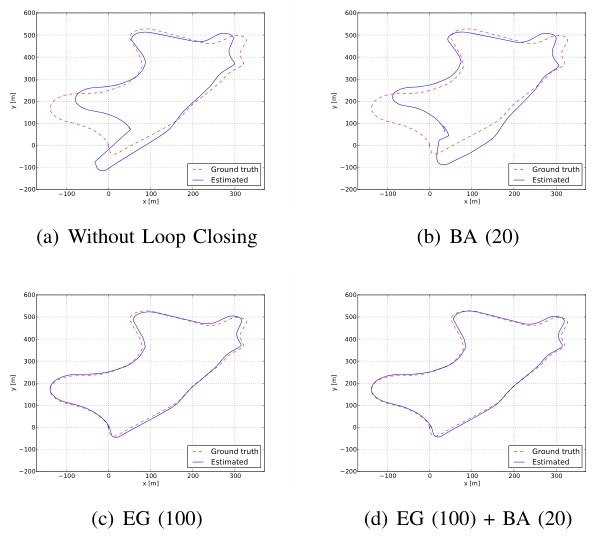
Fig. 13. Comparison of different loop closing strategies in KITTI 09. (a) Without Loop Closing. (b) BA (20). (c) EG (100). (d) EG (100) + BA (20).
图 13. KITTI 09 上不同回环闭合策略的比较。(a) 不做回环闭合。(b) BA (20)。(c) EG (100)。(d) EG (100) + BA (20)。
IX. CONCLUSIONS AND DISCUSSION
A. Conclusions
In this work we have presented a new monocular SLAM system with a detailed description of its building blocks and an exhaustive evaluation in public datasets. Our system has demonstrated that it can process sequences from indoor and outdoor scenes and from car, robot and hand-held motions. The accuracy of the system is typically below 1 cm in small indoor scenarios and of a few meters in large outdoor scenarios (once we have aligned the scale with the ground truth).
本文提出一套新的单目 SLAM 系统,详细描述了它的各个组成模块,并在公开数据集上做了详尽评估。系统表明,它能够处理室内和室外场景,以及车载、机器人和手持运动下的序列。精度在小型室内场景中通常低于 1 厘米,在大型室外场景中为数米(在把尺度与真值对齐之后)。
Currently PTAM by Klein and Murray [4] is considered the most accurate SLAM method from monocular video in real time. It is not coincidence that the backend of PTAM is bundle adjustment, which is well known to be the gold standard method for the offline Structure From Motion problem [2]. One of the main successes of PTAM, and the earlier work of Mouragnon [3], was to bring that knowledge into the robotics SLAM community and demonstrate its real time performance.
目前,Klein 和 Murray 的 PTAM [4] 仍被认为是从单目视频实时运行的最精确 SLAM 方法。PTAM 的后端是束调整,这并非巧合:束调整早已是离线运动恢复结构问题的金标准方法 [2]。PTAM 以及更早 Mouragnon 的工作 [3] 的一个主要贡献,就是把这一认识带进机器人 SLAM 社区,并证明它可以实时运行。
The main contribution of our work is to expand the versatility of PTAM to environments that are intractable for that system. To achieve this, we have designed from scratch a new monocular SLAM system with some new ideas and algorithms, but also incorporating excellent works developed in the past few years, such as the loop detection of Gálvez-López and Tardós [5], the loop closing procedure and covisibility graph of Strasdat et.al [6], [7], the optimization framework g2o by Kuemmerle et. al [37] and ORB features by Rubble et. al [9]. To the best of our knowledge, no other system has demonstrated to work in as many different scenarios and with such accuracy. Therefore our system is currently the most reliable and complete solution for monocular SLAM.
我们工作的主要贡献,是把 PTAM 的通用性扩展到对该系统来说难以处理的环境。为此,我们从零设计了一套新的单目 SLAM 系统,其中有一些新的想法和算法,同时也吸收了过去几年的优秀工作,例如 Gálvez-López 和 Tardós 的回环检测 [5]、Strasdat 等人的回环闭合流程与共视图 [6]、[7]、Kuemmerle 等人的优化框架 g2o [37],以及 Rubble 等人的 ORB 特征 [9]。据我们所知,还没有其他系统表明能在这么多种不同场景中工作,并达到这样的精度。因此,我们的系统目前是单目 SLAM 最可靠、最完整的解决方案。
Our novel policy to spawn and cull keyframes, permits to create keyframes every few frames, which are eventually removed when considered redundant. This flexible map expansion is really useful in poorly conditioned exploration trajectories, i.e. close to pure rotations or fast movements. When operating repeatedly in the same environment, the map only grows if the visual content of the scene changes, storing a history of its different visual appearances. Interesting results for long-term mapping could be extracted analyzing this history.
我们生成和剔除关键帧的新策略,允许每隔几帧就创建关键帧,并在认为它们冗余时最终删掉。这种灵活的地图扩展,在条件不好的探索轨迹中非常有用,例如接近纯旋转或快速运动时。在同一环境中反复运行时,只有场景的视觉内容发生变化,地图才会增长,并保存不同视觉外观的历史。分析这段历史,有可能得到对长期建图有意义的结果。
Finally we have also demonstrated that ORB features have enough recognition power to enable place recognition from severe viewpoint change. Moreover they are so fast to extract and match (without the need of multi-threading or GPU acceleration) that enable real time accurate tracking and mapping.
最后,我们还表明 ORB 特征有足够的识别能力,即使视角变化很大也能做位置识别。而且它们的提取和匹配足够快(不需要多线程或 GPU 加速),因而能够实现实时、准确的跟踪与建图。
B. Sparse/Feature-based vs. Dense/Direct Methods
Recent real-time monocular SLAM algorithms such as DTAM [44] and LSD-SLAM [10] are able to perform dense or semi dense reconstructions of the environment, while the camera is localized by optimizing directly over image pixel intensities. These direct approaches do not need feature extraction and thus avoid the corresponding artifacts. They are also more robust to blur, low-texture environments and high-frequency texture like asphalt [45]. Their denser reconstructions, as compared to the sparse point map of our system or PTAM, could be more useful for other tasks than just camera localization.
近年的实时单目 SLAM 算法,如 DTAM [44] 和 LSD-SLAM [10],能够对环境做稠密或半稠密重建,同时通过直接在图像像素强度上优化来定位相机。这些直接方法不需要提取特征,因而避免了相应的伪影。它们对模糊、低纹理环境以及沥青一类高频纹理也更稳健 [45]。与我们的系统或 PTAM 的稀疏点地图相比,它们更稠密的重建,除了相机定位之外,对其它任务可能更有用。
However, direct methods have their own limitations. Firstly, these methods assume a surface reflectance model that in real scenes produces its own artifacts. The photometric consistency limits the baseline of the matches, typically narrower than those that features allow. This has a great impact in reconstruction accuracy, which requires wide baseline observations to reduce depth uncertainty. Direct methods, if not correctly modeled, are quite affected by rolling-shutter, auto-gain and auto-exposure artifacts (as in the TUM RGB-D Benchmark). Finally, because direct methods are in general very computationally demanding, the map is just incrementally expanded as in DTAM, or map optimization is reduced to a pose graph, discarding all sensor measurements as in LSD-SLAM.
不过,直接方法也有自身的局限。首先,这些方法假定一种表面反射模型,在真实场景中会产生其特有的伪影。光度一致性限制了匹配的基线,通常比特征所允许的更窄。这对重建精度影响很大,因为减少深度不确定性需要宽基线观测。如果建模不当,直接方法会明显受到卷帘快门、自动增益和自动曝光伪影的影响(如在 TUM RGB-D 基准中)。最后,由于直接方法通常计算量很大,地图往往只是像 DTAM 那样增量扩展,或者像 LSD-SLAM 那样把地图优化简化成位姿图,并丢弃全部传感器测量。
In contrast, feature-based methods are able to match features with a wide baseline, thanks to their good invariance to viewpoint and illumination changes. Bundle adjustment jointly optimizes camera poses and points over sensor measurements. In the context of structure and motion estimation, Torr and Zisserman [46] already pointed the benefits of feature-based against direct methods. In this work we provide experimental evidence (see Section VIII-B) of the superior accuracy of feature-based methods in real-time SLAM. We consider that the future of monocular SLAM should incorporate the best of both approaches.
相比之下,基于特征的方法能够在宽基线上匹配特征,这得益于它们对视角和光照变化有较好的不变性。束调整在传感器测量上联合优化相机位姿和空间点。在结构和运动估计的语境里,Torr 和 Zisserman [46] 早已指出基于特征的方法相对直接方法的好处。本文为基于特征的方法在实时 SLAM 中具有更高精度提供了实验证据(见第 VIII-B 节)。我们认为,单目 SLAM 的未来应当把两种途径各自的长处结合起来。
C. Future Work
The accuracy of our system can still be improved incorporating points at infinity in the tracking. These points, which are not seen with sufficient parallax and our system does not include in the map, are very informative of the rotation of the camera [21].
系统的精度仍可通过在跟踪中引入无穷远点来提高。这些点没有被以足够的视差观察到,因而没有被纳入地图,但对相机的旋转非常有信息量 [21]。
Another open way is to upgrade the sparse map of our system to a denser and more useful reconstruction. Thanks to our keyframe selection, keyframes comprise a compact summary of the environment with a very high pose accuracy and rich information of covisibility. Therefore the ORB-SLAM sparse map can be an excellent initial guess and skeleton, on top of which a dense and accurate map of the scene can be built. A first effort in this line is presented in [47].
另一条仍开放的路,是把系统的稀疏地图升级为更稠密、也更有用的重建。得益于我们的关键帧选择,关键帧构成对环境的紧凑摘要,位姿精度很高,并带有丰富的共视信息。因此,ORB-SLAM 的稀疏地图可以作为一个很好的初值和骨架,在此之上再建立场景的稠密、准确地图。这条线上的初步工作见 [47]。
APPENDIX
NON-LINEAR OPTIMIZATIONS
• Bundle Adjustment (BA) [1]:
• Bundle Adjustment (BA) [1]:
Map point 3D locations and keyframe poses , where stands for the world reference, are optimized minimizing the reprojection error with respect to the matched keypoints . The error term for the observation of a map point in a keyframe is:
地图点的三维位置 和关键帧位姿 (其中 表示世界坐标系)被优化,以最小化相对于已匹配关键点 的重投影误差。地图点 在关键帧 中的观测误差项为:
where is the projection function:
其中 是投影函数:
where and are respectively the rotation and translation parts of , and and are the focal length and principle point associated to camera . The cost function to be minimized is:
其中 和 分别是 的旋转和平移部分, 和 是与相机 相关联的焦距和主点。要最小化的代价函数为:
where is the Huber robust cost function and is the covariance matrix associated to the scale at which the keypoint was detected. In case of full BA (used in the map initialization explained in Section IV and in the experiments in Section VIII-E) we optimize all points and keyframes, by the exception of the first keyframe which remain fixed as the origin. In local BA (see section VI-D) all points included in the local area are optimized, while a subset of keyframes is fixed. In pose optimization, or motion-only BA, (see section V) all points are fixed and only the camera pose is optimized.
其中 是 Huber 鲁棒代价函数, 是与关键点被检测时所在尺度相关联的协方差矩阵。在完整 BA 中(用于第 IV 节所述的地图初始化,以及第 VIII-E 节的实验),我们优化全部点和关键帧,但第一帧关键帧保持固定,作为原点。在局部 BA 中(见第 VI-D 节),局部区域内包含的全部点都被优化,同时有一个关键帧子集被固定。在位姿优化,即仅运动 BA 中(见第 V 节),全部点被固定,只优化相机位姿。
• Pose Graph Optimization over Sim(3) Constraints [6]:
• Pose Graph Optimization over Sim(3) Constraints [6]:
Given a pose graph of binary edges (see Section VII-D) we define the error in an edge as:
给定一张由二元边构成的位姿图(见第 VII-D 节),我们把一条边上的误差定义为:
where is the relative transformation between both keyframes computed from the poses just before the pose graph optimization and setting the scale factor to 1. In the case of the loop closure edge this relative transformation is computed with the method of Horn [42]. The [48] transforms to the tangent space, so that the error is a vector in . The goal is to optimize the keyframe poses minimizing the cost function:
其中 是两个关键帧之间的相对 变换,由位姿图优化即将开始时的 位姿计算,并把尺度因子设为 1。对回环闭合边,这一相对变换用 Horn 的方法 [42] 计算。 [48] 变换到切空间,因而误差是 中的向量。目标是优化 关键帧位姿,使代价函数最小:
where is the information matrix of the edge, which, as in [48], we set to the identity. We fix the loop closure keyframe to fix the 7 degrees of gauge freedom. Although this method is a rough approximation of a full BA, we demonstrate experimentally in Section VIII-E that it has significantly faster and better convergence than BA.
其中 是该边的信息矩阵,与 [48] 一样,我们把它设为单位阵。我们固定回环闭合关键帧,以固定 7 个规范自由度。虽然这一方法只是完整 BA 的粗略近似,但我们在第 VIII-E 节用实验表明,它比 BA 收敛明显更快,也更好。
• Relative Sim(3) Optimization:
• Relative Sim(3) Optimization:
Given a set of matches (keypoints and their associated 3D map points) between keyframe 1 and keyframe 2, we want to optimize the relative transformation (see Section VII-B) that minimizes the reprojection error in both images:
给定关键帧 1 与关键帧 2 之间的一组 个匹配 (关键点及其关联的三维地图点),我们要优化相对 变换 (见第 VII-B 节),使两幅图像中的重投影误差最小:
and the cost function to minimize is:
要最小化的代价函数为:
where and are the covariance matrices associated to the scale in which keypoints in image 1 and image 2 were detected. In this optimization the points are fixed.
其中 和 是与图像 1 和图像 2 中关键点被检测时所在尺度相关联的协方差矩阵。在这一优化中,点是固定的。
REFERENCES
参考文献
[1] B. Triggs, P. F. McLauchlan, R. I. Hartley, and A. W. Fitzgibbon, “Bundle adjustment a modern synthesis,” in Vision algorithms: theory and practice, 2000, pp. 298–372.
[2] R. Hartley and A. Zisserman, Multiple View Geometry in Computer Vision, 2nd ed. Cambridge University Press, 2004.
[3] E. Mouragnon, M. Lhuillier, M. Dhome, F. Dekeyser, and P. Sayd, “Real time localization and 3d reconstruction,” in Computer Vision and Pattern Recognition, 2006 IEEE Computer Society Conference on, vol. 1, 2006, pp. 363–370.
[4] G. Klein and D. Murray, “Parallel tracking and mapping for small AR workspaces,” in IEEE and ACM International Symposium on Mixed and Augmented Reality (ISMAR), Nara, Japan, November 2007, pp. 225–234.
[5] D. Gálvez-López and J. D. Tardós, “Bags of binary words for fast place recognition in image sequences,” IEEE Transactions on Robotics, vol. 28, no. 5, pp. 1188–1197, 2012.
[6] H. Strasdat, J. M. M. Montiel, and A. J. Davison, “Scale drift-aware large scale monocular SLAM.” in Robotics: Science and Systems (RSS), Zaragoza, Spain, June 2010.
[7] H. Strasdat, A. J. Davison, J. M. M. Montiel, and K. Konolige, “Double window optimisation for constant time visual SLAM,” in IEEE International Conference on Computer Vision (ICCV), Barcelona, Spain, November 2011, pp. 2352–2359.
[8] C. Mei, G. Sibley, and P. Newman, “Closing loops without places,” in IEEE/RSJ International Conference on Intelligent Robots and Systems (IROS), Taipei, Taiwan, October 2010, pp. 3738–3744.
[9] E. Rublee, V. Rabaud, K. Konolige, and G. Bradski, “ORB: an efficient alternative to SIFT or SURF,” in IEEE International Conference on Computer Vision (ICCV), Barcelona, Spain, November 2011, pp. 2564–2571.
[10] J. Engel, T. Schöps, and D. Cremers, “LSD-SLAM: Large-scale direct monocular SLAM,” in European Conference on Computer Vision (ECCV), Zurich, Switzerland, September 2014, pp. 834–849.
[11] R. Mur-Artal and J. D. Tardós, “Fast relocalisation and loop closing in keyframe-based SLAM,” in IEEE International Conference on Robotics and Automation (ICRA), Hong Kong, China, June 2014, pp. 846–853.
[12] ——, “ORB-SLAM: Tracking and mapping recognizable features,” in MVIGRO Workshop at Robotics Science and Systems (RSS), Berkeley, USA, July 2014.
[13] B. Williams, M. Cummins, J. Neira, P. Newman, I. Reid, and J. D. Tardós, “A comparison of loop closing techniques in monocular SLAM,” Robotics and Autonomous Systems, vol. 57, no. 12, pp. 1188–1197, 2009.
[14] D. Nister and H. Stewenius, “Scalable recognition with a vocabulary tree,” in IEEE Computer Society Conference on Computer Vision and Pattern Recognition (CVPR), vol. 2, New York City, USA, June 2006, pp. 2161–2168.
[15] M. Cummins and P. Newman, “Appearance-only SLAM at large scale with FAB-MAP 2.0,” The International Journal of Robotics Research, vol. 30, no. 9, pp. 1100–1123, 2011.
[16] M. Calonder, V. Lepetit, C. Strecha, and P. Fua, “BRIEF: Binary Robust Independent Elementary Features,” in European Conference on Computer Vision (ECCV), Hersonissos, Greece, September 2010, pp. 778–792.
[17] E. Rosten and T. Drummond, “Machine learning for high-speed corner detection,” in European Conference on Computer Vision (ECCV), Graz, Austria, May 2006, pp. 430–443.
[18] H. Bay, T. Tuytelaars, and L. Van Gool, “SURF: Speeded Up Robust Features,” in European Conference on Computer Vision (ECCV), Graz, Austria, May 2006, pp. 404–417.
[19] D. G. Lowe, “Distinctive image features from scale-invariant keypoints,” International Journal of Computer Vision, vol. 60, no. 2, pp. 91–110, 2004.
[20] A. J. Davison, I. D. Reid, N. D. Molton, and O. Stasse, “MonoSLAM: Real-time single camera SLAM,” IEEE Transactions on Pattern Analysis and Machine Intelligence, vol. 29, no. 6, pp. 1052–1067, 2007.
[21] J. Civera, A. J. Davison, and J. M. M. Montiel, “Inverse depth parametrization for monocular SLAM,” IEEE Transactions on Robotics, vol. 24, no. 5, pp. 932–945, 2008.
[22] C. Forster, M. Pizzoli, and D. Scaramuzza, “SVO: Fast semi-direct monocular visual odometry,” in Proc. IEEE Intl. Conf. on Robotics and Automation, Hong Kong, China, June 2014, pp. 15–22.
[23] O. D. Faugeras and F. Lustman, “Motion and structure from motion in a piecewise planar environment,” International Journal of Pattern Recognition and Artificial Intelligence, vol. 2, no. 03, pp. 485–508, 1988.
[24] W. Tan, H. Liu, Z. Dong, G. Zhang, and H. Bao, “Robust monocular SLAM in dynamic environments,” in IEEE International Symposium on Mixed and Augmented Reality (ISMAR), Adelaide, Australia, October 2013, pp. 209–218.
[25] H. Lim, J. Lim, and H. J. Kim, “Real-time 6-DOF monocular visual SLAM in a large-scale environment,” in IEEE International Conference on Robotics and Automation (ICRA), Hong Kong, China, June 2014, pp. 1532–1539.
[26] D. Nistér, “An efficient solution to the five-point relative pose problem,” IEEE Transactions on Pattern Analysis and Machine Intelligence, vol. 26, no. 6, pp. 756–770, 2004.
[27] H. Longuet-Higgins, “The reconstruction of a plane surface from two perspective projections,” Proceedings of the Royal Society of London. Series B. Biological Sciences, vol. 227, no. 1249, pp. 399–410, 1986.
[28] P. H. Torr, A. W. Fitzgibbon, and A. Zisserman, “The problem of degeneracy in structure and motion recovery from uncalibrated image sequences,” International Journal of Computer Vision, vol. 32, no. 1, pp. 27–44, 1999.
[29] A. Chiuso, P. Favaro, H. Jin, and S. Soatto, “Structure from motion causally integrated over time,” IEEE Transactions on Pattern Analysis and Machine Intelligence, vol. 24, no. 4, pp. 523–535, 2002.
[30] E. Eade and T. Drummond, “Scalable monocular SLAM,” in IEEE Computer Society Conference on Computer Vision and Pattern Recognition (CVPR), vol. 1, New York City, USA, June 2006, pp. 469–476.
[31] H. Strasdat, J. M. M. Montiel, and A. J. Davison, “Visual SLAM: Why filter?” Image and Vision Computing, vol. 30, no. 2, pp. 65–77, 2012.
[32] G. Klein and D. Murray, “Improving the agility of keyframe-based slam,” in European Conference on Computer Vision (ECCV), Marseille, France, October 2008, pp. 802–815.
[33] K. Pirker, M. Ruther, and H. Bischof, “CD SLAM-continuous localization and mapping in a dynamic world,” in IEEE/RSJ International Conference on Intelligent Robots and Systems (IROS), San Francisco, USA, September 2011, pp. 3990–3997.
[34] S. Song, M. Chandraker, and C. C. Guest, “Parallel, real-time monocular visual odometry,” in IEEE International Conference on Robotics and Automation (ICRA), 2013, pp. 4698–4705.
[35] P. F. Alcantarilla, J. Nuevo, and A. Bartoli, “Fast explicit diffusion for accelerated features in nonlinear scale spaces,” in British Machine Vision Conference (BMVC), Bristol, UK, 2013.
[36] X. Yang and K.-T. Cheng, “LDB: An ultra-fast feature for scalable augmented reality on mobile devices,” in IEEE International Symposium on Mixed and Augmented Reality (ISMAR), 2012, pp. 49–57.
[37] R. Kuemmerle, G. Grisetti, H. Strasdat, K. Konolige, and W. Burgard, “g2o: A general framework for graph optimization,” in IEEE International Conference on Robotics and Automation (ICRA), Shanghai, China, May 2011, pp. 3607–3613.
[38] J. Sturm, N. Engelhard, F. Endres, W. Burgard, and D. Cremers, “A benchmark for the evaluation of RGB-D SLAM systems,” in IEEE/RSJ International Conference on Intelligent Robots and Systems (IROS), Vilamoura, Portugal, October 2012, pp. 573–580.
[39] M. Smith, I. Baldwin, W. Churchill, R. Paul, and P. Newman, “The new college vision and laser data set,” The International Journal of Robotics Research, vol. 28, no. 5, pp. 595–599, 2009.
[40] A. Geiger, P. Lenz, C. Stiller, and R. Urtasun, “Vision meets robotics: The KITTI dataset,” The International Journal of Robotics Research, vol. 32, no. 11, pp. 1231–1237, 2013.
[41] V. Lepetit, F. Moreno-Noguer, and P. Fua, “EPnP: An accurate O(n) solution to the PnP problem,” International Journal of Computer Vision, vol. 81, no. 2, pp. 155–166, 2009.
[42] B. K. P. Horn, “Closed-form solution of absolute orientation using unit quaternions,” Journal of the Optical Society of America A, vol. 4, no. 4, pp. 629–642, 1987.
[43] F. Endres, J. Hess, J. Sturm, D. Cremers, and W. Burgard, “3-d mapping with an rgb-d camera,” IEEE Transactions on Robotics, vol. 30, no. 1, pp. 177–187, 2014.
[44] R. A. Newcombe, S. J. Lovegrove, and A. J. Davison, “DTAM: Dense tracking and mapping in real-time,” in IEEE International Conference on Computer Vision (ICCV), Barcelona, Spain, November 2011, pp. 2320–2327.
[45] S. Lovegrove, A. J. Davison, and J. Ibanez-Guzmán, “Accurate visual odometry from a rear parking camera,” in IEEE Intelligent Vehicles Symposium (IV), 2011, pp. 788–793.
[46] P. H. Torr and A. Zisserman, “Feature based methods for structure and motion estimation,” in Vision Algorithms: Theory and Practice. Springer, 2000, pp. 278–294.
[47] R. Mur-Artal and J. D. Tardos, “Probabilistic semi-dense mapping from highly accurate feature-based monocular SLAM,” in Robotics: Science and Systems (RSS), Rome, Italy, July 2015.
[48] H. Strasdat, “Local Accuracy and Global Consistency for Efficient Visual SLAM,” Ph.D. dissertation, Imperial College, London, October 2012.
Raúl Mur Artal was born in Zaragoza, Spain in 1989. He received the Industrial Engineering degree (mention in Industrial Automation and Robotics) in 2012 and the M.S. degree in Systems and Computer Engineering in 2013 from the University of Zaragoza, where he is currently working towards the PhD. degree with the I3A Robotics, Perception and Real-Time Group. His research interests include Visual Localization and Long-Term Mapping.
Raúl Mur Artal,1989 年生于西班牙萨拉戈萨。他于 2012 年获得工业工程学位(工业自动化与机器人方向),并于 2013 年获得系统与计算机工程硕士学位,均来自萨拉戈萨大学;目前他正在该校 I3A 机器人、感知与实时研究组攻读博士学位。研究兴趣包括视觉定位和长期建图。
J. M . M. Montiel was born in Arnedo, Spain, in 1967. He received the M.S. and Ph.D. degrees in electrical engineering from the Universidad de Zaragoza, Spain, in 1992 and 1996, respectively. He is currently a Full Professor with the Departamento de Informática e Ingeniería de Sistemas, Universidad de Zaragoza, where he is in charge of Perception and Computer Vision research grants and courses. His current interests include, real-time vision localization and semantic mapping for rigid and non rigid environments, and the transference of this technology to robotic and nonrobotic application domains. Prof. Martínez Montiel is a member of the I3A Robotics, Perception, and Real-Time Group. He has been awarded several Spanish MEC grants to fund research at the University of Oxford, UK, and at Imperial College London, UK.
J. M . M. Montiel,1967 年生于西班牙阿内多。他于 1992 年和 1996 年分别在西班牙萨拉戈萨大学获得电气工程硕士和博士学位。他目前是萨拉戈萨大学 Departamento de Informática e Ingeniería de Sistemas 的正教授,负责感知与计算机视觉方面的研究项目与课程。当前兴趣包括刚性和非刚性环境中的实时视觉定位与语义建图,以及把这项技术转移到机器人与非机器人应用领域。Martínez Montiel 教授是 I3A 机器人、感知与实时研究组的成员。他曾获得多项西班牙教育部(MEC)资助,分别在英国牛津大学和伦敦帝国学院开展研究。
Juan D. Tardós was born in Huesca, Spain, in 1961. He earned the M.S. and Ph.D. degrees in electrical engineering from the University of Zaragoza, Spain, in 1985 and 1991, respectively. He is Full Professor with the Departamento de Informática e Ingeniería de Sistemas, University of Zaragoza, where he is in charge of courses in robotics, computer vision, and artificial intelligence. His research interests include SLAM, perception and mobile robotics. Prof. Tardós is a member of the I3A Robotics, Perception, and Real-Time Group.
Juan D. Tardós,1961 年生于西班牙韦斯卡。他于 1985 年和 1991 年分别在西班牙萨拉戈萨大学获得电气工程硕士和博士学位。他是萨拉戈萨大学 Departamento de Informática e Ingeniería de Sistemas 的正教授,负责机器人、计算机视觉和人工智能课程。研究兴趣包括 SLAM、感知和移动机器人。Tardós 教授是 I3A 机器人、感知与实时研究组的成员。