Optimal Mistake Bounds for Transductive Online Learning
Optimal Mistake Bounds for Transductive Online Learning
直推在线学习的最优错误界
Zachary Chase Kent State University 𝚣𝚌𝚑𝚊𝚜𝚎𝟸 @ 𝚔𝚎𝚗𝚝 . 𝚎𝚍𝚞 \mathtt{zchase2@kent.edu} Steve Hanneke Purdue University 𝚜𝚝𝚎𝚟𝚎 . 𝚑𝚊𝚗𝚗𝚎𝚔𝚎 @ 𝚐𝚖𝚊𝚒𝚕 . 𝚌𝚘𝚖 \mathtt{steve.hanneke@gmail.com} Shay Moran Departments of Mathematics, Computer Science, and Data and Decision Sciences Technion – Israel Institute of Technology; Google Research 𝚜𝚖𝚘𝚛𝚊𝚗 @ 𝚝𝚎𝚌𝚑𝚗𝚒𝚘𝚗 . 𝚊𝚌 . 𝚒𝚕 \mathtt{smoran@technion.ac.il} Jonathan Shafer MIT 𝚜𝚑𝚊𝚏𝚎𝚛𝚓𝚘 @ 𝚖𝚒𝚝 . 𝚎𝚍𝚞 \mathtt{shaferjo@mit.edu}
Abstract
摘要
We resolve a 30-year-old open problem concerning the power of unlabeled data in online learning by tightly quantifying the gap between transductive and standard online learning. In the standard setting, the optimal mistake bound is characterized by the Littlestone dimension of the concept class (Littlestone 1987). We prove that in the transductive setting, the mistake bound is at least . This constitutes an exponential improvement over previous lower bounds of , , and , due respectively to Ben-David et al. 1995; Ben-David et al. 1997, and Hanneke et al. 2023. We also show that this lower bound is tight: for every , there exists a class of Littlestone dimension with transductive mistake bound . Our upper bound also improves upon the best known upper bound of from Ben-David et al. 1997. These results establish a quadratic gap between transductive and standard online learning, thereby highlighting the benefit of advance access to the unlabeled instance sequence. This contrasts with the PAC setting, where transductive and standard learning exhibit similar sample complexities.
我们解决了一个历时三十年的开放问题:无标注数据在在线学习中究竟有多大力量——通过紧致刻画直推在线学习与标准在线学习之间的差距。在标准设定下,最优错误界由概念类 的 Littlestone 维 刻画(Littlestone 1987)。我们证明:在直推设定下,错误界至少为 。这相对于先前由 Ben-David 等 1995、Ben-David 等 1997 以及 Hanneke 等 2023 给出的 、 与 下界是指数级改进。我们还证明该下界是紧的:对每个 ,都存在 Littlestone 维为 、且直推错误界为 的概念类。我们的上界也改进了 Ben-David 等 1997 给出的当时最好上界 。这些结果确立了直推与标准在线学习之间的二次差距,从而凸显提前获知无标注实例序列的益处。这与 PAC 设定形成对照:在 PAC 中,直推学习与标准学习的样本复杂度相近。
1 Introduction
1 引言
Contents
The transductive model is a basic and well-studied framework in learning theory, dating back to the early works of Vapnik. It has been investigated both in statistical and online settings, and is motivated by the principle that to make good predictions on a specific set of test instances, one need not construct a fully general classifier that performs well on the entire domain — including points that may never actually appear. Rather, it may be sufficient to tailor predictions for a fixed, known set of instances.
目录
直推模型是学习理论中基础且研究充分的框架,可追溯到 Vapnik 的早期工作。它在统计设定与在线设定中都得到研究,其动机是:若只想在一组特定的测试实例上做出好预测,未必需要构造在整个定义域——包括那些可能永远不会出现的点——上都表现良好的完全一般分类器。针对一个固定且已知的实例集合定制预测,往往就够了。
This perspective naturally connects to a broader question in learning theory: what is the value of unlabeled data? In the transductive setting, the learner is given the sequence of unlabeled test instances in advance and is then required to predict their labels one by one. Thus, the transductive model can be viewed as a natural formalization of learning with unlabeled data: the test instances are known in advance, but their labels are not. The central question is whether such prior access to the unlabeled sequence can help reduce the number of prediction mistakes — compared to the standard online model, where the instances arrive and are labeled one at a time.
这一视角自然联系到学习理论中一个更宽的问题:无标注数据的价值是什么?在直推设定中,学习器预先获知无标注测试实例序列,再逐一预测其标签。因此,直推模型可视为「带无标注数据学习」的一种自然形式化:测试实例事先已知,但其标签未知。核心问题是:相比标准在线模型(实例逐个到达并被标注),这种对无标注序列的先验访问能否减少预测错误次数。
Recall for instance that in the standard PAC[^1] model of supervised learning, there are cases where access to unlabeled data is not helpful. Indeed, the ‘‘hard population distributions’’ used to prove the standard VC[^2] lower bound are constructed by taking a fixed and known marginal distribution over a VC-shattered set. Namely, the cases that are hardest to learn in the PAC setting include ones where the learner knows the marginal distribution over the domain, and can therefore generate as much unlabeled data as it wishes. And yet, in those cases, access to unlabeled data provides no acceleration compared to an algorithm (like ERM[^3]) that does not use unlabeled data.
回顾标准 PAC[^1] 监督学习模型:存在若干情形,无标注数据并无帮助。的确,用于证明标准 VC[^2] 下界的「困难总体分布」,是通过对一个 VC 可打散集合取固定且已知的边缘分布构造的。也就是说,PAC 中最难学的情形包含学习器已知定义域上边缘分布、因而可任意生成无标注数据的情形。即便如此,在这些情形中,使用无标注数据相对于不使用无标注数据的算法(如 ERM[^3])并不能带来加速。
Seeing as unlabeled data is often a lot easier to obtain than labeled data, there have been considerable efforts to understand when and to what extent can access to unlabeled data accelerate learning.[^4]
鉴于无标注数据往往远比有标注数据容易获得,已有大量工作试图弄清:何时、以及在多大程度上,访问无标注数据能够加速学习。[^4]
In particular, it is natural to ask, for which plausible models of learning is access to unlabeled data beneficial? Online learning (Littlestone 1987) is perhaps the model of learning that is most-extensively studied in learning theory after the PAC model and its variants. Therefore, the general question considered in this paper is:
特别地,一个自然的问题是:在哪些合理的学习模型中,访问无标注数据是有益的?在线学习(Littlestone 1987)或许是继 PAC 及其变体之后在学习理论中被研究得最充分的模型。因此,本文考虑的一般问题是:
Question 1.
Quantitatively, how much (if at all) is access to unlabeled data beneficial for learning in the online learning setting?
问题 1。
定量地看,访问无标注数据对在线学习设定中的学习究竟有多大益处(若有的话)?
This question is naturally instantiated by comparing transductive online learning — where the learner has advance access to the full sequence of unlabeled instances — with standard online learning, where no such access is given. This perspective has also been adopted in prior work: for example, Kakade and Kalai 2005, Cesa-Bianchi and Shamir 2013, and Hoi et al. 2021 (Section 7.3) all describe transductive online learning as a setting in which the learner has access to “unlabeled data”. We thus refine the question above as follows:
把该问题具体化,就是比较直推在线学习——学习器可预先获知完整无标注实例序列 ——与标准在线学习——没有这种访问。先前工作也采用这一视角:例如 Kakade 与 Kalai 2005、Cesa-Bianchi 与 Shamir 2013,以及 Hoi 等 2021(第 7.3 节),都把直推在线学习描述为学习器可访问「无标注数据」的设定。我们因此把上述问题细化如下:
Question 2.
Quantitatively, how much (if at all) is learning in the transductive online learning setting easier than learning in the standard online learning setting? Specifically, how much is the optimal number of mistakes in the transductive setting smaller than in the standard setting?
问题 2。
定量地看,直推在线学习设定下的学习究竟比标准在线学习容易多少(若有的话)?具体而言,直推设定下的最优错误次数比标准设定小多少?
Addressing this question, our main result (Theorem 1.1) states that the optimal number of mistakes in the transductive setting (with access to unlabeled data) is at most quadratically smaller than in the standard setting (without unlabeled data). Furthermore, there are hypothesis classes for which a quadratic gap is achieved.
针对这一问题,我们的主要结果(定理 1.1)表明:直推设定(可访问无标注数据)下的最优错误次数,至多比标准设定(无无标注数据)小一个二次因子。并且存在实现二次差距的假设类。
1.1 Setting: Standard vs. Transductive Online Learning
1.1 设定:标准与直推在线学习
Standard online learning (Littlestone 1987) is a zero-sum, perfect- and complete-information game played over rounds between two players, a learner and an adversary. The game is played with respect to a domain set and a hypothesis class (consisting of functions ), where , and are fixed and known to both players. The game proceeds as follows.
标准在线学习(Littlestone 1987)是一个在 轮中由两名玩家——学习器与对手——进行的零和、完全且完备信息博弈。博弈相对于定义域 与假设类 (由函数 组成)进行,其中 、 与 固定且双方已知。博弈进程如下。
For each round :
The adversary selects an instance and sends it to the learner.
The learner selects a prediction and sends it to the adversary.
The adversary selects a label and sends it to the learner. The selected label must be realizable, meaning that .
List of games 1 The standard online learning setting.
对每一轮 :
对手选择一个实例 并发送给学习器。
学习器选择一个预测 并发送给对手。
对手选择一个标签 并发送给学习器。所选标签必须可实现,即存在 使得 。
博弈列表 1 标准在线学习设定。
The number of mistakes for a learner and an adversary is . We are interested in understanding the optimal number of mistakes, which is
学习器 与对手 的错误次数为 。我们关心的是最优错误次数,即
where and are the set of all deterministic adversaries and learners, respectively.[^5] It is well known that is characterized by the Littlestone dimension, namely, (see Theorems 5.7 and 5.6).
其中 与 分别是所有确定性对手与学习器的集合。[^5] 众所周知, 由 Littlestone 维刻画,即 (见定理 5.7 与定义 5.6)。
The transductive online learning setting (Ben-David et al. 1995; Ben-David et al. 1997) is similar, except that the learner has access to the full sequence of unlabeled instances in advance. Namely,
直推在线学习设定(Ben-David 等 1995;Ben-David 等 1997)与之类似,区别在于学习器可预先获知完整的无标注实例序列。即:
The adversary selects a sequence and sends it to the learner.
For each round :
The learner selects a prediction and sends it to the adversary.
The adversary selects a label and sends it to the learner. The selected label must be realizable, meaning that .
List of games 2 The transductive online learning setting.
对手选择一个序列 并发送给学习器。
对每一轮 :
学习器选择一个预测 并发送给对手。
对手选择一个标签 并发送给学习器。所选标签必须可实现,即存在 使得 。
博弈列表 2 直推在线学习设定。
The optimal number of mistakes for the transductive setting is defined exactly as before,
直推设定下的最优错误次数定义与此前完全相同:
with the only difference between the standard quantity and the transductive quantity being in how the game is defined.
标准量 与直推量 之间的唯一差别,在于博弈如何定义。
1.2 Main Result
1.2 主要结果
Notice that for every hypothesis class , . Indeed, in the transductive setting the adversary declares the sequence at the start of the game. This reduces the number of mistakes because the transductive adversary is less powerful (it cannot adaptively alter the sequence mid-game), and also because the transductive learner is more powerful (it has more information).[^6]
注意对每个假设类 ,都有 。的确,在直推设定中对手在博弈开始时就声明序列 。这会减少错误次数,因为直推对手更弱(不能在博弈中途自适应地改序列),也因为直推学习器更强(信息更多)。[^6]
While for some classes , we study the largest possible separation. The best previous lower bound on , due to Hanneke et al. 2023, states that for every class ,
虽然对某些类有 ,我们研究的是最大可能的分离。先前关于 的最好下界由 Hanneke 等 2023 给出:对每个类 ,
where . In the other direction, Ben-David et al. 1997 constructed[^7] a class such that and
其中 。另一方面,Ben-David 等 1997 构造[^7] 了一个类 ,满足 且
This left an exponential gap between the best known lower and upper bounds on , namely versus . Our main result closes this gap:
这使得关于 的已知最好下界与上界之间留下指数级缺口,即 对 。我们的主要结果弥合了这一缺口:
Theorem 1.1(Main result).
- • For every hypothesis class, where
定理 1.1(主要结果)。
- • 对每个假设类, 其中
- • On the other hand, for everythere exists a hypothesis classwithand
- • 另一方面,对每个都存在假设类满足且
This result is stated in considerably greater detail in Theorems 6.1 and 8.1.
该结果在定理 6.1 与定理 8.1 中有更详细的陈述。
1.3 Related Works
1.3 相关工作
The notion of transductive inference as a more efficient alternative to inductive inference in statistical learning theory was introduced by Vapnik 1979; Vapnik 2006; Gammerman et al. 1998; Chapelle et al. 1999. The online learning setting is due to Littlestone 1987, who also proved that the optimal number of mistakes is characterized by the Littlestone dimension (see Theorem 5.7).
把直推推断作为统计学习理论中相对归纳推断更高效的替代方案这一观念,由 Vapnik 1979;Vapnik 2006;Gammerman 等 1998;Chapelle 等 1999 引入。在线学习设定由 Littlestone 1987 提出,他还证明最优错误次数由 Littlestone 维刻画(见定理 5.7)。
The transductive online learning setting studied in the current paper, was first defined by Ben-David et al. 1995, who used the name worst sequence off-line model. Among other results, they showed a lower bound of on the number of mistakes required to learn a class with Littlestone dimension . The authors subsequently presented an exponentially stronger lower bound of in Ben-David et al. 1997. However, understanding where the optimal number of mistakes is situated within the range remained an open question.
本文研究的直推在线学习设定最早由 Ben-David 等 1995 定义,当时称为最坏序列离线模型。除其他结果外,他们给出了学习 Littlestone 维为 的类所需错误次数的 下界。作者随后在 Ben-David 等 1997 中给出指数更强的 下界。然而,最优错误次数落在区间 中的何处,仍是开放问题。
Kakade and Kalai 2005 presented an oracle-efficient algorithm for the transductive online learning setting, and may have been the first to use that name. Their result was subsequently improved upon by Cesa-Bianchi and Shamir 2013.
Kakade 与 Kalai 2005 给出了直推在线学习设定的 oracle 高效算法,或许是最早使用该名称的工作。其结果随后由 Cesa-Bianchi 与 Shamir 2013 改进。
The present work is most similar to that of Hanneke et al. 2023 which, among other results, gave a quadratically-stronger mistake lower bound of for classes with Littlestone dimension in the transductive online setting. The proof of our lower bound utilizes some of their ideas, but yields a quantitative improvement by combining it with some new ideas.
与本文最接近的是 Hanneke 等 2023:除其他结果外,他们为 Littlestone 维为 的类在直推在线设定下给出了二次更强的 错误下界。我们下界的证明利用了他们的部分想法,但通过与新想法结合得到了定量改进。
Hanneke et al. 2024 studied a setting of multi-class transductive online learning where the number of possible labels is unbounded.
Hanneke 等 2024 研究了可能标签数无界的多类直推在线学习设定。
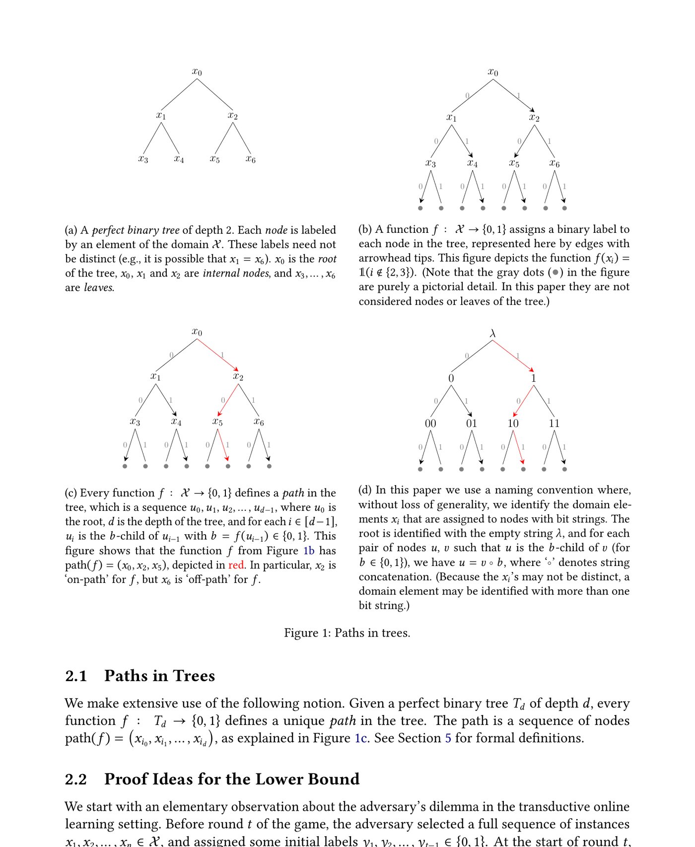
(a) A perfect binary tree of depth . Each node is labeled by an element of the domain . These labels need not be distinct (e.g., it is possible that ). is the root of the tree, , and are internal nodes, and are leaves.
(a) 深度为 的完美二叉树。每个结点由定义域 的一个元素标注。这些标注不必互异(例如可以有 )。 是树的根,、 与 是内部结点, 是叶子。
2 Technical Overview
2 技术概览
In this section we explain some of the main ideas in our proofs. Formal definition appear in Section 5. Full formal statements of the results, as well as detailed rigorous proofs, appear in Sections 6, 7, and 8.
本节解释证明中的若干主要想法。形式定义见第 5 节。结果的完整形式陈述与详尽严格证明见第 6、7、8 节。
2.1 Paths in Trees
2.1 树中的路径
We make extensive use of the following notion. Given a perfect binary tree of depth , every function defines a unique path in the tree. The path is a sequence of nodes , as explained in Fig. 1(c). See Section 5 for formal definitions.
我们大量使用如下概念。给定深度为 的完美二叉树 ,每个函数 在树中定义一条唯一的路径。该路径是结点序列 ,如图 1(c) 所示。形式定义见第 5 节。
2.2 Proof Ideas for the Lower Bound
2.2 下界的证明想法
We start with an elementary observation about the adversary’s dilemma in the transductive online learning setting. Before round of the game, the adversary selected a full sequence of instances , and assigned some initial labels . At the start of round , the adversary must consider the version space,
我们先从一个关于直推在线学习设定中对手困境的初等观察开始。在第 轮之前,对手已选定完整实例序列 ,并赋给了若干初始标签 。在第 轮开始时,对手必须考虑版本空间
If all assign for some , then the adversary has no choice but to assign the label . Otherwise, the adversary can force a mistake at time . Namely, after seeing the learner’s prediction , the adversary can assign , incrementing the number of learner mistakes by .
若所有 对某个 都满足 ,则对手别无选择,只能赋标签 。否则,对手可以在时刻 强制一次错误。即:在看到学习器的预测 后,对手可赋 ,使学习器错误次数加 1。
But “just because you can, doesn’t mean you should”. If the adversary is greedy and forces a mistake at time , they may pay dearly for that later. As an extreme example, consider the case where there is a single that assigns , and all other functions assign . If the learner selects and the adversary forces a mistake at time , the version space at all subsequent times will be , and the adversary will be prevented from forcing any further mistakes.
但「能做不意味着该做」。若对手贪婪地在时刻 强制错误,日后可能付出沉重代价。极端例子:若 中仅有一个 满足 ,而其余函数都赋 。若学习器选 且对手在 强制错误,则后续所有时刻 的版本空间都是 ,对手再也无法强制任何错误。
A natural strategy for the adversary is therefore to be greedy up to a certain limit. Namely, at each time the adversary computes the ratio[^8]
因此对手的一种自然策略是:贪婪到某个限度为止。即在每个时刻 ,对手计算比率[^8]
If for some parameter (“the version space is not too unbalanced”), then the adversary forces a mistake. Otherwise, the adversary assigns the majority label, i.e., . This ensures that the version space does not shrink too fast:
若对某个参数 有 (「版本空间不太不平衡」),则对手强制错误。否则对手赋多数标签,即 。这保证版本空间不会收缩过快:
- • If no mistake is forced, then , and
- • 若未强制错误,则 ,并且
- • If a mistake is forced, .
- • 若强制了错误,则 。
In particular, at the end of the game, the version space is of size
特别地,博弈结束时版本空间 的大小满足
where is the number of mistakes that the adversary forces and is the length of the sequence. The class has size because , and by removing functions from the class if necessary (which can only make learning easier), we may assume without loss of generality that . Namely, the class precisely shatters a Littlestone tree of depth such that for every assignment of labels to a root-to-leaf path in the tree, the class contains exactly one function that agrees with that assignment (see Definition 5.6 for detail).
其中 是对手强制的错误次数, 是序列长度。因为 ,类的大小 ;必要时可从类中删去函数(这只会让学习更容易),因而可无损一般性地假定 。即:该类恰好打散一棵深度为 的 Littlestone 树,使得对树中任一条根到叶路径上的任意标签赋值,类中恰有一个与之相符的函数(细节见定义 5.6)。
Notice that we have not yet specified how the adversary selects the sequence . While the adversary’s labeling strategy is extremely simple (determined by the ratio and the prediction ), constructing of the sequence requires some care, to ensure that it has the following two properties:
注意我们尚未说明对手如何选择序列 。虽然对手的标注策略极其简单(由比率 与预测 决定),构造序列 却需要小心,以确保它具有以下两条性质:
- • Property I: The length of the sequence satisfies , and
- • 性质 I: 序列长度 满足 ,并且
- • Property II: For every sequence of predictions selected by the learner, the resulting sequence of labels selected by the adversary are consistent with some function such that contains all the nodes in .[^9]
- • 性质 II: 对学习器所选的每一预测序列 ,对手所得标签序列 都与某个 一致,且 包含 中的全部结点。[^9]
These properties can be achieved by carefully simulating all possible execution paths of the adversary.
这些性质可通过仔细模拟对手所有可能的执行路径来达成。
Observe that if then the sequence of labels uniquely identifies the function within the class . Hence, Property II and the assumption imply that at the end of the game, the version space has cardinality
观察到:若 ,则标签序列 在类 内唯一标识函数 。因此,性质 II 与假定 意味着博弈结束时版本空间 的基数为
Combining Property I (), Eqs. 2 and 1, and choosing gives
结合性质 I()、式 2 与式 1,并取 ,得到
which implies
从而推出
as desired.
此即所需。
2.3 Proof Ideas for the Upper Bound
2.3 上界的证明想法
In this section we explain the main ideas in the proof of Theorem 8.1, which states that for every , there exists a class of Littlestone dimension that is learnable in the transductive online setting with a mistake bound of .
本节解释定理 8.1 证明中的主要想法。该定理断言:对每个 ,都存在 Littlestone 维为 的类,可在直推在线设定下以 的错误界学习。
Of course, not every Littlestone class satisfies this property. For instance, the set of all functions has Littlestone dimension , but the adversary can force the learner to make mistakes when learning this class in the transductive setting.[^10] So our task in this proof is to construct a class that is especially easy to learn in the transductive setting (i.e., learnable with mistakes), while still being hard (requiring mistakes) in the standard setting.
当然,并非每个 Littlestone 类都满足这一性质。例如,所有函数 构成的集合 Littlestone 维为 ,但对手可在直推设定下迫使学习器犯 次错误。[^10] 因此本证明的任务是:构造一个在直推设定下特别容易学(即可用 次错误学会)、而在标准设定下仍然困难(需要 次错误)的类。
2.3.1 Sparse Encodings are Easy to Guess
We start with an elementary observation. Consider the following two bit strings:
2.3.1 稀疏编码易于猜测
我们从一个初等观察开始。考虑以下两个比特串:
Both of these strings encode the number . However, one of the encodings is much easier to guess than the other: suppose we are tasked with guessing the bits in an encoding of an integer between and . We guess the bits one at a time, and after each guess, an adaptive adversary tells us whether our guess was correct.
这两个串都编码数字 。然而其中一个编码远比另一个容易猜:假设任务是猜测某个介于 与 之间整数的编码中的各位。我们一次猜一位,每次猜测后自适应对手告诉我们是否正确。
Now, if the bit string is a binary encoding, the task is hard. Each bit can either be or , regardless of the values of the previous bits, and so the adversary can force a mistake on every bit. On the other hand, if we know that the string is a one-hot encoding, there exists an attractive strategy — always guess . This ensures that we will make at most mistake.
若比特串是二进制编码,任务就难:每一位无论先前各位取值如何都可以是 或 ,对手可在每一位上强制错误。反之,若已知该串是独热编码,则存在有吸引力的策略——始终猜 。这保证我们至多犯 次错误。
Note that at the end of the guessing game we have learned the same amount of information (for a number between and , we learned bits of information), but the number of mistakes is very different ( mistakes vs. mistake).
注意:猜测游戏结束时我们学到的信息量相同(对 到 之间的数,学到 比特信息),但错误次数截然不同( 次对 次)。
2.3.2 Construction of the Hypothesis Class
We now describe a construction of a hypothesis class that is easy to learn in the transductive setting, using the idea of a sparse encoding. Recall that a class has Littlestone dimension at least (Definition 5.6 in Section 5) if there exists a Littlestone tree of depth such that for every there exists such that the values on the path of agree with . More formally, , and in particular . Thus, when constructing a class that shatters a specific Littlestone tree of depth , we need to define functions . For each function , the on-path values of the function are fixed (fully determined by ), while for the remaining values there is complete freedom (for the nodes that are off-path we may assign any values ).
2.3.2 假设类的构造
我们现在描述一个在直推设定下易于学习的假设类构造,其核心是稀疏编码的想法。回顾:若存在深度为 的 Littlestone 树,使得对每个 都存在 ,其在路径上的取值与 一致,则类 的 Littlestone 维至少为 (定义 5.6,第 5 节)。更形式地,,特别地 。因此,在构造打散一棵特定深度 的 Littlestone 树的类时,需要定义 个函数 。对每个函数 ,路径上的取值是固定的(完全由 决定),而其余取值则完全自由(对路径外结点 ,可任意赋 )。
Perhaps the simplest way to construct a class of Littlestone dimension is simply to assign all on-path values as required, and assign to all other values. Namely, if is a prefix of then , and otherwise . In a sense, this is the ‘minimal’ class of Littlestone dimension for a specific Littlestone tree.[^11]
构造 Littlestone 维为 的类,最简单的方式或许是:按要求赋所有路径上取值,其余一律赋 。即:若 是 的前缀则 ,否则 。在某种意义上,这是针对特定 Littlestone 树的「极小」Littlestone 维 类。[^11]
Observe that the ‘minimal’ class does not have the desired property of being easy to learn in the transductive setting.[^12] However, a certain variation of the ‘minimal’ class that embeds a sparse encoding does satisfy the requirement. In this variation, on-path value of the function are assigned as they must (as determined by ), while the off-path values are sampled independently using a biased coin, such that each of them is with high probability, but has a small probability of being . The probability is chosen carefully so that the class satisfies some simple combinatorial properties, as described further in Sections 2.3.6 and 8.2.
可以观察到:「极小」类并不具有「在直推设定下易学」这一期望性质。[^12] 然而,「极小」类的某种嵌入了稀疏编码的变体确实满足要求。在该变体中, 的路径上取值仍按 必须赋的方式赋值,而路径外取值则用有偏硬币独立采样:每个以高概率为 ,但有小概率为 。概率被仔细选取,使该类满足若干简单组合性质,细节见第 2.3.6 节与第 8.2 节。
2.3.3 Naïve Learning Strategy
We now explain in broad strokes how the probabilistic construction of the hypothesis class in Section 2.3.2 is useful for learning with few mistakes in the transductive setting.
2.3.3 朴素学习策略
我们现在粗线条地说明:第 2.3.2 节中假设类的概率构造,如何有助于在直推设定下以较少错误学习。
Notice that when predicting labels for the ‘minimal’ class with nodes in breadth-first order, the learner knows at each step whether they are labeling an on-path or off-path node, because the learner has already seen the correct labels for all ancestors of the current node. For off-path nodes, the learner knows that the true label is , so it never makes mistakes on off-path nodes, but it also gains no new information when the true labels for off-path nodes are revealed. No risk, but no reward either. Instead, all the information about the true labeling function is revealed only at on-path nodes, where the adversary has complete freedom to assign labels and force mistakes. That’s why the adversary can force mistakes.
注意:当按广度优先顺序为「极小」类的结点预测标签时,学习器在每一步都知道自己在标注路径上还是路径外结点,因为当前结点所有祖先的正确标签都已见过。对路径外结点,学习器知道真标签是 ,因而从不在路径外结点上犯错,但路径外真标签揭晓时也不获得新信息——无风险,亦无回报。关于真标注函数的全部信息只在路径上结点揭晓,而对手在那里可完全自由赋标签并强制错误。这就是对手能强制 次错误的原因。
For the randomly-chosen class, when predicting labels for off-path nodes, the learner may still safely predict a label of . But the reasoning for this is quite different. Conceptually, every off-path label is part of a sparse codeword that identifies the correct labeling function.[^13] Because the coin is biased, each bit of the codeword is easy to guess (it is likely to be ), but every time that the adversary reveals that the true label for an off-path node is indeed , the learner gains a small (nonzero) amount of information about the true labeling function. Additionally, when the adversary selects an off-path label of , that reveals a lot of information about the true labeling function (such labels are rare in the hypothesis class), and therefore the adversary cannot force many off-path mistakes. Overall, the information about the true labeling function is ‘smeared’ throughout all labels of the tree (s and s, on-path and off-path).[^14]
对随机选取的类,在预测路径外结点的标签时,学习器仍可安全地预测 。但理由大不相同。概念上,每个路径外标签都是识别正确标注函数的稀疏码字的一部分。[^13] 因为硬币有偏,码字的每一位都容易猜(很可能是 ),但每当对手揭示某个路径外结点的真标签确实是 ,学习器就获得关于真标注函数的少量(非零)信息。此外,当对手选择路径外标签为 时,这揭示了大量关于真标注函数的信息(这类标签在假设类中稀少),因而对手不能强制太多路径外错误。总体而言,关于真标注函数的信息被「涂抹」在树的所有标签上( 与 ,路径上与路径外)。[^14]
Thus, the naïve general strategy for the learner when using the probabilistically-constructed class is to learn most of the information about the true labeling function by observing off-path labels. By the time the learner reaches an on-path node, it hopefully has already learned enough about the true labeling function in order to make a good prediction on that node.
因此,使用概率构造类时学习器的朴素一般策略是:通过观察路径外标签来学习关于真标注函数的大部分信息。待学习器到达路径上结点时,希望已经学到足够多,从而能在该结点上做出好预测。
However, making this general strategy work requires overcoming some very substantial obstacles:
然而,要使这一一般策略奏效,需要克服若干相当实质性的障碍:
- Recall that in the transductive setting, the adversary can present the nodes of the tree in any order of its choosing — it does not have to present the tree in breadth-first order. The naïve strategy works only if the learner sees many off-path nodes before it sees most on-path nodes. But what happens if the adversary decides to present many on-path nodes near the beginning of the sequence? To handle this, the learner incorporates a strategy we call ‘danger zone minimization’, as described in Section 2.3.4.
- 回顾:在直推设定中,对手可以按任意自选顺序呈现树的结点——不必按广度优先。朴素策略仅当学习器在见到多数路径上结点之前先见到许多路径外结点时才奏效。但若对手决定在序列开头呈现许多路径上结点会怎样?为处理这一点,学习器引入我们称为「危险区最小化」的策略,见第 2.3.4 节。
- Another, equally problematic, issue also arises from the fact that the sequence presented by the adversary might not be in breadth-first order. Recall that breadth-first order[^15] has the property that for every node in the sequence, all the ancestors of appear before in the sequence. This means that by the time the learner needs to predict a label for , the learner knows whether is on-path or off-path for the true labeling function. But what happens if the adversary presents before some of ’s ancestors? Or omits some of ’s ancestors from the sequence altogether? In this case the learner doesn’t know if is on-path or off-path, and this presents a double hazard. One hazard is that the leaner doesn’t know what label to predict for — if is off-path, the learner can simply predict , but if it is on-path it must do something more elaborate. The second hazard is that, after seeing the correct label for , it is not clear what the learner can infer from it. If is off-path, its label should be interpreted as part of a sparse encoding of the labeling function. But if is on-path, the interpretation must be entirely different. To overcome this challenge, the learner incorporates a strategy we call ‘splitting experts’, described in Section 2.3.5.
- 另一个同样棘手的问题也来自对手呈现的序列可能不是广度优先。回顾:广度优先顺序[^15] 具有如下性质:对序列中每个结点 , 的所有祖先都在序列中出现于 之前。这意味着学习器需要为 预测标签时,已知道对真标注函数而言 在路径上还是路径外。但若对手在 的某些祖先之前呈现 ,或根本从序列中省略某些祖先?此时学习器不知道 在路径上还是路径外,从而面临双重风险。其一是不知道该为 预测什么标签——若 在路径外,学习器可简单预测 ,但若在路径上则必须做更复杂的事。其二是:见到 的正确标签后,不清楚能从中推断什么。若 在路径外,其标签应解释为标注函数稀疏编码的一部分;若 在路径上,解释必须完全不同。为克服这一挑战,学习器引入我们称为「分裂专家」的策略,见第 2.3.5 节。
- Limiting off-path mistakes. Thanks to the coin’s bias, most off-path nodes have a true label of . Nonetheless, each function in the hypothesis class still has an expected number of off-path nodes labeled , so the learner can afford to misclassify only a vanishing fraction of them! To limit the number of mistakes, the learner extracts information from the sparse encoding and executes a ‘transition to Halving’ strategy, as described in Section 2.3.6.
- 限制路径外错误。得益于硬币的偏置,多数路径外结点的真标签是 。尽管如此,假设类中每个函数仍期望有 个标注为 的路径外结点,因而学习器只能错分其中消失比例的一小部分!为限制错误次数,学习器从稀疏编码中提取信息,并执行「过渡到折半」策略,见第 2.3.6 节。
2.3.4 Danger Zone Minimization
Utilizing information from the ‘sparse encoding’ of the off-path nodes to make good predictions for on-path nodes requires that the learner first see the true labels for many off-path nodes. Until that happens, the learner expects to make many mistakes on on-path nodes. However, whether a node is on-path or off-path is not fixed in advanced — the adversary may decide this adaptively, in response to the learners predictions.
2.3.4 危险区最小化
利用路径外结点「稀疏编码」中的信息来对路径上结点做出好预测,要求学习器先见到许多路径外结点的真标签。在此之前,学习器预期会在路径上结点上犯许多错误。然而,结点在路径上还是路径外并非事先固定——对手可响应学习器的预测自适应地决定。
Danger zone minimization is a strategy used by the learner, to force the adversary to assign few nodes in the beginning of the sequence as on-path (otherwise, if initial nodes are assigned to be on-path by the adversary, then the learner will make few mistakes on those nodes). This is analogous to the standard Halving algorithm (7), but instead of minimizing the cardinality of the set of consistent hypotheses (the ‘version space’), the learner minimizes a subset of the domain (the ‘danger zone’).
危险区最小化是学习器使用的一种策略,用以迫使对手在序列开头把较少结点赋为路径上(否则,若开头结点被对手赋为路径上,则学习器在这些结点上会犯较少错误)。这类似于标准折半算法(7),但学习器最小化的不是一致假设集合(「版本空间」)的基数,而是定义域的一个子集(「危险区」)。
Concretely, at the beginning of the game the learner initializes a set consisting of the first instances in the sequence selected by the adversary. This set represents the ‘danger zone’ — nodes in the beginning of the sequence that have not been labeled yet, that might be on-path, and that are not ancestors of a previously-labeled on-path node.[^16] To predict a label for an instance , the learner selects a label such that if is wrong, the danger zone will shrink by at least . That is, for , if the set of -descendants of has cardinality , the learner predicts . Then, if the adversary selects , that implies that all -descendants of are off-path for the true labeling functions. Therefore, the learner removes all -descendants of from the danger zone, and the new cardinality is . This guarantees that the learner can make at most such mistakes before the danger zone is empty.[^17]
具体地,博弈开始时学习器初始化集合 ,由对手所选序列 的前 个实例组成。该集合表示「危险区」——序列开头尚未标注、可能在路径上、且不是先前已标注路径上结点之祖先的结点。[^16] 为实例 预测标签时,学习器选择 ,使得若 错误,危险区将至少缩小 。即:对 ,若 的 -后代集合 满足 ,则学习器预测 。于是,若对手选 ,则意味着 的所有 -后代对真标注函数都在路径外。因此学习器从危险区移除所有这些 -后代,新基数 。这保证学习器在危险区变空之前至多犯 次此类错误。[^17]
If neither nor have cardinality at least , the learner predicts . If and is on-path for the true labeling function, then the learner updates the danger zone to be ,[^18] again shrinking the danger zone by a factor of at most . Otherwise, if and is off-path, then it was an off-path node labeled (which is rare), and the learner can afford to misclassify it (see Section 2.3.6).
若 与 的基数都达不到 ,学习器预测 。若 且 对真标注函数在路径上,则学习器把危险区更新为 ,[^18] 再次把危险区缩小至多 倍。否则,若 且 在路径外,则这是一个标注为 的路径外结点(稀少),学习器可以承受错分它(见第 2.3.6 节)。
2.3.5 Splitting Experts
The danger zone minimization strategy requires that the learner know whether the node being classified is on-path or off-path for the true labeling function. However, if appears in the sequence before some of its ancestors, the learner does not know this. To overcome this difficulty, the learner implements a variant of the standard multiplicative weights algorithm using splitting experts. This means that initially there is a single expert executing danger zone minimization. When a node is reached for which danger zone minimization requires knowing whether is on-path or off-path and that information is not yet evident, each expert is split into two experts, one of which continues the execution of danger zone minimization under the assumption that is on-path, and the other under the opposite assumption. Thus, at each point in time, there exists precisely one expert for which all path-related assumptions are correct, and therefore that expert will make at most mistakes. The multiplicative weights algorithm guarantees that the overall number of mistakes will be linear in the number of mistakes of the best expert, i.e., .
2.3.5 分裂专家
危险区最小化策略要求学习器知道正在分类的结点 对真标注函数在路径上还是路径外。然而,若 在其某些祖先之前出现在序列中,学习器并不知道这一点。为克服这一困难,学习器使用分裂专家实现标准乘性权重算法的一个变体。这意味着一开始只有一个专家在执行危险区最小化。当到达某个结点 ,危险区最小化需要知道 在路径上还是路径外而该信息尚未明确时,每个专家分裂为两个:一个在假定 在路径上的前提下继续危险区最小化,另一个在相反假定下继续。因此,在每个时刻,恰存在一个专家其所有路径相关假定都正确,因而该专家至多犯 次错误。乘性权重算法保证总体错误次数与最佳专家的错误次数成线性关系,即 。
2.3.6 Transition to Halving
The hypothesis class is engineered such that it satisfies the following property: there are at most functions in the hypothesis class that agree with any set of labels, or that agree that a set of nodes are all off-path and labeled (this follows from Lemma 8.2).
2.3.6 过渡到折半
假设类被设计成满足如下性质:与任意 个标签一致的函数,或一致认定某 个结点都在路径外且标注为 的函数,在假设类中至多有 个(这由引理 8.2 推出)。
Therefore, once the true labels for the first instances have been revealed, or once off-path labels of have been revealed (whichever happens first), the learner can transition to halving: stop doing danger zone minimization, and instead predict the labels for the remaining nodes using the standard Halving algorithm (7) on the subset of the hypothesis class that survived. Halving on functions is guaranteed to make at most mistakes (A.1).
因此,一旦前 个实例 的真标签已揭晓,或一旦已揭晓 个路径外标签 (以先发生者为准),学习器就可以过渡到折半:停止危险区最小化,转而在幸存的假设类子集上用标准折半算法(7)预测其余结点的标签。在 个函数上折半,保证至多犯 次错误(A.1)。
However, seeing as the learner lacks information on which nodes are off-path, it uses experts, and each expert maintains different path-related assumptions. Thus, each expert decides separately at which point to transition to Halving. The unique expert that makes only correct assumptions will transition ‘at the right time’. That expert will make at most mistakes during danger zone minimization, and then at most additional mistakes during halving.
然而,由于学习器缺少哪些结点在路径外的信息,它使用专家,且每个专家维护不同的路径相关假定。因此,每个专家各自决定何时过渡到折半。那个只做正确假定的唯一专家会在「正确时机」过渡。该专家在危险区最小化期间至多犯 次错误,随后在折半期间再至多犯 次错误。
2.4 Some Intuition for the Quantity
2.4 关于量 的若干直觉
We briefly sketch where the quantity arises from. This is a back-of-the-envelope calculation without proof, intended purely as an aid for intuition. Suppose we assigned off-path labels of with probability instead of . Consider a sequence of leaves. For any sequence of labels , taking , there exist roughly
我们简要勾勒 这一量从何而来。这是没有证明的粗略估算,仅作直觉辅助。假设我们以概率 而非 赋路径外标签 。考虑由 片叶子组成的序列 。对任意标签序列 ,取 ,大约存在
functions in the class for which these leaves are off-path and which agree with the labels . Therefore, the adversary can force at least mistakes.
个函数使这些叶子在路径外且与标签 一致。因此对手至少可强制 次错误。
Similarly, for the sequence consisting of all the nodes in the tree of depth at most in breadth-first order, the adversary can force a mistake on every on-path node while assigning a label of to all off-path nodes, for a total of mistakes. This is true because for any assignment of on-path labels, the fraction of functions which agree with the on-path labels that assign a label of to all off-path nodes is roughly
类似地,对由深度至多 的树中全部结点按广度优先组成的序列 ,对手可在每个路径上结点强制错误,同时给所有路径外结点赋标签 ,总共 次错误。这成立是因为:对任意路径上标签赋值,与路径上标签一致、且给所有路径外结点赋 的函数所占比例大约为
so in particular for any labeling of the on-path nodes there exists a function in the class that agrees with that labeling and assigns to all off-path nodes.
因而特别地,对路径上结点的任意标注,类中都存在与之相符并给所有路径外结点赋 的函数。
Therefore, for any , we obtain a lower bound of on the number of mistakes. For any , , giving a lower bound of . Choosing to minimize the lower bound will in fact yield a matching upper bound of , as we show in this paper. This completes our overview of the upper bound.
因此,对任意 ,我们得到错误次数的下界 。对任意 ,,从而得到 下界。选取 以最小化下界,事实上将给出匹配的 上界,如本文所示。至此完成上界概览。
3 Directions for Future Work
3 未来工作方向
Following are some interesting open questions:
以下是若干有趣的开放问题:
- Does there exist an efficient learning algorithm that achieves the upper bound of Theorem 8.1? One needs to be careful about the definition of efficiency here, but one possible formalization is as follows. Does there exist a learning algorithm and a sequence of classes , such that for every : • , and • Given as input the index and a sequence , the algorithm runs in time and makes at most mistakes assuming the labels are realizable by .
- 是否存在达到定理 8.1 的 上界的高效学习算法?这里需要小心定义「高效」,一种可能的形式化如下。是否存在学习算法 与一列类 ,使得对每个 :• ,并且 • 以指标 与序列 为输入,算法 在时间 内运行,并在标签可由 实现的假定下至多犯 次错误。
- Is there a tradeoff between the cardinality of the domain and the upper bound on the number of mistakes? We used a domain of size roughly in order to obtain our upper bound of . Is it possible to get the same bound with a domain of size ?
- 定义域 的基数与错误次数上界之间是否存在权衡?我们使用大小约为 的定义域以获得 上界。能否在定义域大小为 时得到同样的界?
- Obtaining more precise asymptotics; for example, is there (an explicit) constant such that the optimal transductive mistake bound is ?
- 获得更精确的渐近;例如,是否存在(显式的)常数 ,使得最优直推错误界为 ?
4 Organization
4 组织结构
Formal definitions appear in Section 5. Formal statements and proofs for the lower bound and upper bound appear in Section 6 and Section 8, respectively. Optimal sequence length is discussed in Section 7.
形式定义见第 5 节。下界与上界的形式陈述与证明分别见第 6 节与第 8 节。最优序列长度在第 7 节讨论。
5 Preliminaries
5 预备知识
5.1 Basic Notation
5.1 基本记号
Notation 5.1.
, i.e., . and denote logarithm to base and , respectively.
记号 5.1。
,即 。 与 分别表示以 与 为底的对数。
Notation 5.2(Sequences).
Let be a set and . For a sequence , we write to denote the subsequence . If then denotes the empty sequence, which is also denoted by . We use the notation .
记号 5.2(序列)。
设 为集合,。对序列 ,我们写 表示子序列 。若 ,则 表示空序列,也记作 。我们使用记号 。
5.2 Standard Online Learning
5.2 标准在线学习
Let be a set, and let be a collection of functions called a hypothesis class. A learner strategy or simply learner for the standard online learning game (1) is a function
设 为集合,设 为一族函数,称为假设类。标准在线学习博弈(1)的学习器策略或简称学习器是一个函数
where is the number of rounds in the game. The set of all such learner strategies is denoted . An adversary strategy or simply adversary for the standard online learning game is a pair of functions
其中 是博弈轮数。所有此类学习器策略的集合记为 。标准在线学习博弈的对手策略或简称对手是一对函数
The set of all such adversary strategies is denoted .
所有此类对手策略的集合记为 。
Semantically, the interpretation of these strategies is that in each round of 1, the adversary selects an instance
语义上,这些策略的解释是:在博弈 1 的每一轮 ,对手选择一个实例
then the learner makes a prediction
然后学习器做出预测
and finally, the adversary assigns a label
最后,对手赋一个标签
The adversary’s function must satisfy realizability, meaning that there exists such that
对手的函数 必须满足可实现性,即存在 使得
The number of mistakes in a game with rounds and hypothesis class between learner and adversary is
在假设类为 、 轮的博弈中,学习器 与对手 之间的错误次数为
5.3 Transductive Online Learning
5.3 直推在线学习
Given and as in Section 5.2, a learner strategy for the transductive online learning setting (2) is a function
给定与第 5.2 节相同的 与 ,直推在线学习设定(2)的学习器策略是一个函数
where is the number of rounds in the game. An adversary strategy consists of a sequence and an adversary labeling strategy, which is a function
其中 是博弈轮数。对手策略由序列 与对手标注策略组成,后者是一个函数
The sets of all such learner and adversary strategies are denoted and respectively.
所有此类学习器与对手策略的集合分别记为 与 。
Semantically, the interpretation of these strategies is that at the start of 2, the adversary selects the sequence . Then, in each round , the learner makes a prediction
语义上,这些策略的解释是:在博弈 2 开始时,对手选定序列 。然后在每一轮 ,学习器做出预测
and then the adversary assigns a label
随后对手赋一个标签
Exactly as in Section 5.2, the adversary’s function must satisfy realizability, namely,
与第 5.2 节完全相同,对手的函数 必须满足可实现性,即
and the number of mistakes in a game with sequence length and hypothesis class between learner and adversary is
而在序列长度为 、假设类为 的博弈中,学习器 与对手 之间的错误次数为
5.4 Mistake Bounds
5.4 错误界
In this paper, we study optimal mistake bounds, or the optimal number of mistakes, which is the value of 1 and 2. For , the optimal number of mistakes in a game with hypothesis class and sequence length is,
本文研究最优错误界,或最优错误次数,即博弈 1 与博弈 2 的值。对 ,在假设类为 、序列长度为 的博弈中,最优错误次数为
The optimal number of mistakes for hypothesis class is
假设类 的最优错误次数为
Remark 5.3.
As is common in learning theory literature, in both 1 and 2, we take the sets and to be the sets of all (deterministic) functions. In this paper, we do not consider randomized strategies. By allowing arbitrary functions, we ignore issues relating to computability.
注记 5.3。
与学习理论文献中常见做法一样,在博弈 1 与博弈 2 中,我们取 与 为所有(确定性)函数的集合。本文不考虑随机策略。通过允许任意函数,我们忽略与可计算性相关的问题。
5.5 Trees
5.5 树
Definition 5.4(Notation for binary trees).
Let . A perfect binary tree of depth is a collection of nodes, which we identify with the collection of binary strings
定义 5.4(二叉树记号)。
设 。深度为 的完美二叉树是 个结点的集合,我们将其等同于二进制串的集合
The empty string, denoted , is a member of and is called the root of the tree. Every string is called a leaf. The depth of a node , denoted , is the length of as a string, namely, the integer such that .
空串,记作 ,属于 ,称为树的根。每个串 称为叶子。结点 的深度记作 ,即 作为串的长度,也就是使 的整数 。
For two nodes , we say that is a parent of , and that is a child of , if or , where denotes string concatenation. More fully, for , we say that is a -child of if .
对两个结点 ,若 或 (其中 表示串连接),则称 是 的父结点, 是 的子结点。更完整地,对 ,若 ,则称 是 的 -子结点。
Recursively, we define that is an ancestor of and that is a descendant of , and write , if one of the following holds:
递归地,我们定义 是 的祖先、 是 的后代,并写 ,若下列之一成立:
- • , or
- • ,或
- • .
- • 。
For , we say that is a -descendant of , denoted , if is a descendant of the -child of .
对 ,若 是 的 -子结点的后代,则称 是 的 -后代,记作 。
A function specifies a particular root-to-leaf path in the tree (see Fig. 1). The on-path nodes for are the set of nodes on that root-to-leaf path, as in the following definition.
函数 在树 中指定一条特定的根到叶路径(见图 1)。 的路径上结点是该根到叶路径上的 个结点,如下定义。
Definition 5.5(Paths in a binary tree).
Let , . Let be a node in . The path to is the unique sequence such that is the root, , and is a child of for all .
定义 5.5(二叉树中的路径)。
设 ,。设 为 中的结点。到 的路径是唯一序列 ,使得 为根,,且对所有 , 是 的子结点。
Let be a function. The path of is the unique sequence such that is the root, and for each , . Namely, is the -child of .
设 为函数。 的路径是唯一序列 ,使得 为根,且对每个 ,。即 是 的 -子结点。
For a node and a function , we write if and there exists such that . Otherwise, we write .
对结点 与函数 ,若 且存在 使 ,则写 。否则写 。
For a node and a set of functions , we write if
对结点 与函数集 ,若下列成立则写 :
Otherwise, we write .
否则写 。
5.6 Littlestone Dimension
5.6 Littlestone 维
Definition 5.6(Littlestone 1987).
Let be a set, let , and let . We say that shatters the binary tree if there exists a mapping given by such that for every there exists such that
定义 5.6(Littlestone 1987)。
设 为集合,设 ,设 。若存在映射 由 给出,使得对每个 都存在 满足
The Littlestone dimension of , denoted , is the supremum over all such that there exists a Littlestone tree of depth that is shattered by .
的 Littlestone 维记作 ,是所有使 打散某棵深度为 的 Littlestone 树的 的上确界。
Note that by defining the Littlestone dimension this way, every class with Littlestone dimension contains at least functions.
注意按此方式定义 Littlestone 维时,每个 Littlestone 维为 的类至少包含 个函数。
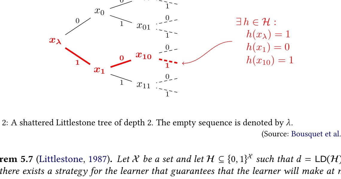
Figure 2: A shattered Littlestone tree of depth 2. The empty sequence is denoted by . (Source: Bousquet et al. 2021)
图 2:一棵深度为 2 的被打散 Littlestone 树。空序列记作 。(来源:Bousquet 等 2021)
Theorem 5.7(Littlestone 1987).
Let be a set and let such that . Then there exists a strategy for the learner that guarantees that the learner will make at most mistakes in the standard (non-transductive) online learning setting, regardless of the adversary’s strategy and of the number of instances to be labeled. Furthermore, there exists an adversary that forces every learner to make at least mistakes.
定理 5.7(Littlestone 1987)。
设 为集合,设 满足 。则存在学习器策略,保证学习器在标准(非直推)在线学习设定下至多犯 次错误,无论对手策略以及待标注实例数 如何。此外,存在对手迫使每个学习器至少犯 次错误。
6 Lower Bound
6 下界
6.1 Statement
6.1 陈述
Our lower bound states the following.
我们的 下界陈述如下。
Theorem 6.1(Lower bound).
There exists a constant as follows. Let , , let be a set, and let be a hypothesis class with . Then there exist a sequence of length and an adversary that always selects the sequence and uses a simple adaptive labeling strategy (as in 1), such that for every learning rule ,
定理 6.1(下界)。
存在常数 如下。设 ,,设 为集合,设 为满足 的假设类。则存在长度为 的序列 ,以及始终选择该序列 并使用简单自适应标注策略(如算法 1)的对手 ,使得对每个学习规则 ,
Furthermore, for every integer ,
此外,对每个整数 ,
Remark 6.2.
The assumption implies that for all , shatters a Littlestone tree of depth . Thus, the lower bound of Eq. 3 in Theorem 6.1 immediately implies that for every there exists a sequence of length such that the adversary that presents the sequence and assigns labels using the simple labeling strategy of 1 ensures that for every learner ,
注记 6.2。
假定 意味着对所有 , 打散一棵深度为 的 Littlestone 树。因此,定理 6.1 中式 3 的下界立即蕴含:对每个 ,存在长度为 的序列 ,使得呈现序列 并用算法 1 的简单标注策略赋标签的对手 保证对每个学习器 ,
See Section 2.2 for a general overview of Theorem 6.1 and the main proof ideas. In the following subsections we prove Theorem 6.1. 1 gives an explicit construction of the adversary that witnesses the lower bound, using 2 as a subroutine. We start with presenting some initial observations about the behavior of these algorithms in Section 6.2.
定理 6.1 的一般概览与主要证明想法见第 2.2 节。以下各小节证明定理 6.1。算法 1 给出见证下界的对手的显式构造,并以算法 2 为子程序。我们从第 6.2 节中关于这些算法行为的若干初步观察开始。
See 2.
send to learner
for :
receive from learner
y_{t}\leftarrow\left\{\begin{array}[]{ll}y_{\mathsf{maj}}&r_{t}\notin[\varepsilon,1-\varepsilon]\\ 1-\hat{y}_{t}&\text{otherwise}\end{array}\right.
send to learner
List of algorithmFloats 1 The strategy for the adversary that achieves the lower bound in Theorem 6.1. Note that while the construction of the sequence is not entirely trivial, the adversary’s strategy for labeling this sequence is very simple.
见算法 2。
send to learner
for :
receive from learner
y_{t}\leftarrow\left\{\begin{array}[]{ll}y_{\mathsf{maj}}&r_{t}\notin[\varepsilon,1-\varepsilon]\\ 1-\hat{y}_{t}&\text{otherwise}\end{array}\right.
send to learner
算法列表 1 达到定理 6.1 下界的对手策略。注意:虽然序列 的构造并非完全平凡,对手对该序列的标注策略却非常简单。
A set of classes indexed by bit strings.
A set of nodes to be processed.
while :
Pop an arbitrary element from and add it to the output sequence.
for :
\mathcal{Y}\leftarrow\left\{\begin{array}[]{ll}\{0,1\}&\big(r\in[\varepsilon,1-\varepsilon]\big)\land\big(|b|<M\big)\\ \{\mathds{1}\mathopen{}\left(r\geq 1/2\right)\mathclose{}\}&\text{otherwise}\end{array}\right. Adversary will force mistakes on the first balanced nodes.
for :
b^{\prime}\leftarrow\left\{\begin{array}[]{ll}b&|\mathcal{Y}|=1\\ b\circ y&|\mathcal{Y}|=2\end{array}\right. Restrict class to agree with . If splitting the class in two to force a mistake then create new indices.
if : If is on-path for and it has a -child, add that child to .
return
List of algorithmFloats 2 A subroutine of 1 for selecting the sequence .
由比特串索引的一类集合。
待处理结点集合。
while :
从 弹出任意元素并加入输出序列。
for :
\mathcal{Y}\leftarrow\left\{\begin{array}[]{ll}\{0,1\}&\big(r\in[\varepsilon,1-\varepsilon]\big)\land\big(|b|<M\big)\\ \{\mathds{1}\mathopen{}\left(r\geq 1/2\right)\mathclose{}\}&\text{otherwise}\end{array}\right. 对手将在前 个平衡结点上强制错误。
for :
b^{\prime}\leftarrow\left\{\begin{array}[]{ll}b&|\mathcal{Y}|=1\\ b\circ y&|\mathcal{Y}|=2\end{array}\right. 将类限制为与 一致。若为强制错误而把类一分为二,则创建新指标。
if : 若 对 在路径上且有 -子结点,则将该子结点加入 。
return
算法列表 2 算法 1 中用于选择序列 的子程序。
6.2 Analysis of the Adversary
6.2 对手的分析
Claim 6.3.
Let , let , and let be a hypothesis class. Consider an execution of as in 2 that produces a sequence . Then:
断言 6.3。
设 ,设 ,设 为假设类。考虑如算法 2 中产生序列 的 的一次执行。则:
(a) For all,is a subsequence of.
(a) 对所有,是的子序列。
(b) The lengthof the sequence satisfies, where.
(b) 序列长度满足,其中。
Proof.
(a) Fix . It suffices to show that for all , if then . Proceed by induction on . For the base case , the claim holds because . For the induction step, assume the claim holds for . Let , we prove that . Assume (otherwise, there is nothing to prove). Because appears in the sequence , it must have been added to before it was added to . The only place where items that are not are added to is in the line . Namely, there exist an index and a bit such that (note that because was added to the sequence before ). If we are done. Otherwise, note that is the parent of , and therefore . By the induction hypothesis, . This concludes the proof.
证明。
(a) 固定 。只需证明:对所有 ,若 则 。对 用归纳法。基础情形 成立,因为 。归纳步骤:假定断言对 成立。设 ,我们证明 。假定 (否则无需证明)。因为 出现在序列 中,它必在被加入 之前被加入 。非 的元素被加入 的唯一位置是行 。即:存在指标 与比特 使 (注意 ,因为 在 之前被加入序列)。若 则完成。否则注意 是 的父结点,因而 。由归纳假设,。证毕。
(b) Items are added to the sequence only if they were previously added to . By induction on , for each in the sequence, there is at most one iteration of the “while ” loop in which is added to . The base case holds because is the root, which is added to before the while loop, and is never added to within that loop because the line “” can only add non-empty bit strings. For the induction step, if the claim holds for all natural numbers such that then it holds for . Indeed, for , can be added to only via the line “”, and only in the iteration of the while loop where is the parent of in the tree . In that iteration, the parent of is popped from , which implies that was added to in some previous iteration of the while loop (), and is no longer in after being popped. By the induction hypothesis, will never be added to again, and therefore in all subsequent iterations of the while loop will not be the parent of , so cannot be added to in subsequent iterations via the line “”. Furthermore, if a node is added to in some iteration of the while loop, then it remains in for the duration of that iteration. So for all , there is precisely one execution of the line “” that adds to . Namely, there is precisely one point in time during the execution of 2 in which , , and the line “” is executed resulting in . Consider a function that maps to the value of the index during the unique execution of the line “” that adds to . Namely, if had some value when was added to , then . Notice that “” is executed only if the condition is satisfied in the previous line. Furthermore, the line “” ensures that the node being added to satisfies , namely Consequently, for any class that is a subset of ; in particular, because the only way that might be modified later during the execution of 2 is by removing elements, it follows that when the line “” is executed and in all subsequent times. However, for any class . This implies that maps at most nodes to each bit string. In other words, for any bit string , the size of the preimage satisfies . The condition “” in 2 ensures that , namely, for . Thus, as desired. ∎
(b) 元素仅在先前被加入 后才会被加入序列 。对 用归纳法:对序列中每个 ,「while 」循环中至多有一次迭代把 加入 。基础情形 成立,因为 是根,在 while 循环之前被加入 ,且 从不在该循环内被加入 ,因为行「」只能加入非空比特串。归纳步骤:若断言对所有满足 的自然数 成立,则对 也成立。的确,对 , 只能经由行「」加入 ,且仅在 while 循环中 为树 中 之父的那次迭代。在该迭代中, 的父结点 从 弹出,这意味着 在先前某次 while 迭代中被加入 (),弹出后不再在 中。由归纳假设, 再也不会被加入 ,因而在后续所有 while 迭代中 都不会是 的父结点,故 不能在后续迭代中经由该行加入 。此外,若结点 在某次 while 迭代中被加入 ,则它在该迭代期间一直留在 中。因此对所有 ,恰有一次执行行「」把 加入 。即:在算法 2 的执行中,恰有一个时刻满足 、,且执行该行后导致 。考虑把 映射到把 加入 的那次唯一执行行「」期间指标 取值的函数 。即:若加入 时 取值为 ,则 。注意「」仅在前一行条件 成立时执行。此外,行「」保证被加入 的结点 满足 ,即 因此对 的任何子类 都有 ;特别地,因为算法 2 后续执行中修改 的唯一方式是删除元素,故在执行该行时及之后所有时刻都有 。然而对任何类 ,。这意味着 至多把 个结点映射到每个比特串。换言之,对任何比特串 ,原像大小满足 。算法 2 中的条件「」保证 ,即 对某个 。于是 此即所需。 ∎
Claim 6.4.
Let , let , and let be a hypothesis class. Consider an execution of as in 1. Let
断言 6.4。
设 ,设 ,设 为假设类。考虑如算法 1 中 的一次执行。设
be the sequence of hypothesis classes created by TransductiveAdversary, let
为 TransductiveAdversary 创建的假设类序列,设
be the set of indices where TransductiveAdversary forces a mistake, and let
为 TransductiveAdversary 强制错误的指标集合,设
be the sequence of collections created by the subroutine ConstructSequence (2). If then
为子程序 ConstructSequence(算法 2)创建的集合序列。若 ,则
Proof.
Proceed by induction on . The base case is satisfied, because . For the induction step, assume that for some . We prove that .
证明。
对 用归纳法。基础情形 成立,因为 。归纳步骤:假定对某个 有 。我们证明 。
Let be the label assigned to by TransductiveAdversary. Then
设 为 TransductiveAdversary 赋给 的标签。则
Consider the iteration of the while loop in ConstructSequence that starts with . By the induction hypothesis, . Therefore, in this iteration of the while loop, there will be an iteration of the “for ” loop where . In that iteration, by construction of and . Therefore, in the iteration of the “for ” loop in which ,
考虑 ConstructSequence 中以 开始的 while 循环迭代。由归纳假设,。因此在该 while 迭代中,将有一次「for 」循环的迭代满足 。在该迭代中,由 与 的构造有 。因此在「for 」循环中 的那次迭代里,
The class is then added to in the line “”. Furthermore, no class is ever removed from . So , as desired. ∎
类 随后在行「」被加入 。此外,从不从 中移除任何类。故 ,此即所需。∎
Claim 6.5.
Let , let , and let be a hypothesis class. Consider an execution of as in 1 where the adversary constructs a sequence of nodes and a sequence of classes . Let
断言 6.5。
设 ,设 ,设 为假设类。考虑如算法 1 中 的一次执行,其中对手构造结点序列 与类序列 。设
be the set of indices where TransductiveAdversary forces a mistake, and assume that . Then for all there exists such that
为 TransductiveAdversary 强制错误的指标集合,并假定 。则对所有 都存在 使得
- , and
- ,并且
- ,
- ,
Proof.
Proceed by induction on . For the base case , notice that , , and .
证明。
对 用归纳法。基础情形 :注意 ,,且 。
For the induction step, assume the claim holds for some , and take such that and ; we prove that the claim holds for as well.
归纳步骤:假定断言对某个 成立,取 使 且 ;我们证明断言对 也成立。
Consider the iteration of the while loop in ConstructSequence in which is added to the sequence (i.e., the iteration starting with ). By 6.4 and the assumption , . Hence, within this iteration of the while loop, there is an iteration of the “for ” loop such that . By construction, the set always contains the label predicted by the adversary, so . Consider the iteration of the “for ” loop such that . By the induction hypothesis, , and since , it follows that . Seeing as , in the last line of this iteration of the “for ” loop, the node is added to . This guarantees that will eventually be popped from and added to the sequence returned by ConstructSequence. Once a node has been added to the sequence, it is never removed.
考虑 ConstructSequence 中把 加入序列的 while 循环迭代(即以 开始的迭代)。由断言 6.4 与假定 ,。故在该 while 迭代内,存在「for 」循环的一次迭代使 。由构造,集合 总包含对手预测的标签,故 。考虑「for 」循环中 的那次迭代。由归纳假设,,又因为 ,故 。由于 ,在该「for 」迭代的最后一行,结点 被加入 。这保证 最终会从 弹出并加入 ConstructSequence 返回的序列。结点一旦加入序列就不再被移除。
Notice that , satisfying Item 1. Therefore, it remains to show Item 2, namely, to show that .
注意 ,满足第 1 项。因此只需证明第 2 项,即证明 。
Indeed, by the induction hypothesis, , and in the iteration of the “for ” discussed above, , , and . Hence,
的确,由归纳假设,,而在上述「for 」迭代中,,,且 。故
Seeing as This implies that
由于 ,这蕴含
Item 2 follows from the inclusion . ∎
第 2 项由包含关系 推出。∎
6.3 Proof
6.3 证明
Finally, we complete the proof of the lower bound.
最后,我们完成下界的证明。
Proof of Theorem 6.1.
Fix and assume . Seeing as , shatters the tree . By replacing with a suitable subset of of cardinality , renaming the elements in the domain of to nodes of , and restricting the domain of each function in to , assume without loss of generality that , , and shatters .
定理 6.1 的证明。
固定 并假定 。由于 , 打散树 。通过把 换成基数为 的合适子集、把 定义域中的元素重命名为 的结点,并把每个函数的定义域限制到 ,可无损一般性地假定 、,且 打散 。
Consider the loop “for ” in 1, and let
考虑算法 1 中的循环「for 」,并设
be the set of indices where the adversary forces a mistake, such that the learner makes at least mistakes. Let , and assume for contradiction that .
为对手强制错误的指标集合,因而学习器至少犯 次错误。设 ,并反设 。
By 6.5, there exists such that (i.e., is a leaf in ) and , namely,
由断言 6.5,存在 使 (即 是 的叶子)且 ,即
Seeing as is a leaf,
由于 是叶子,
By construction,
由构造,
and is not empty. Fix some . By Item (a) in 6.3, is a subsequence of , so
且 非空。固定某个 。由断言 6.3 的第 (a) 项, 是 的子序列,故
Seeing as shatters and , if two functions agree on the labels for all nodes in , then . We conclude that and .
由于 打散 且 ,若两个函数 在 中所有结点上的标签一致,则 。我们结论 且 。
Consider the loop “for ” in 1. For each ,
考虑算法 1 中的循环「for 」。对每个 ,
$$|\mathcal{H}{t}|\geq\begin{cases}\varepsilon\cdot|\mathcal{H}{t-1}|&t\in S\
(1-\varepsilon)\cdot|\mathcal{H}_{t-1}|&t\notin S.\end{cases}$$
Hence,
因此,
where the final line holds because , , and
其中最后一行成立是因为 ,,以及
for our choice of . Rearranging Section 6.3 yields
对我们所选的 。重排第 6.3 节得到
This is a contradiction to the assumption . We conclude that an adversary following 1 satisfies
这与假定 矛盾。我们结论:遵循算法 1 的对手 满足
as desired.
此即所需。
To establish the “furthermore” part of the theorem, fix a length . Let be the largest integer such that and . By Eq. 7, there exists some sequence on which the adversary can force every learning rule to make at least mistakes. By Theorem 7.2, this implies that there exists a sequence of length on which the adversary can force every learning rule to make at least mistakes. Namely,
为确立定理的「此外」部分,固定长度 。设 为满足 且 的最大整数。由式 7,存在某个序列使对手可迫使每个学习规则至少犯 次错误。由定理 7.2,这蕴含存在长度为 的序列,使对手可迫使每个学习规则至少犯同样多次错误,因而
as in Eq. 4. ∎
如式 4。∎
7 Sequence Length
7 序列长度
In this section, we show that if there exists a sequence on which the adversary can force mistakes, then a sequence of length is sufficient, and this upper bound is tight for some classes.[^19]
本节证明:若存在对手可在其上强制 次错误的序列,则长度 的序列已足够,且该上界对某些类是紧的。[^19]
Definition 7.1(Minimal sequence).
Let be a set, let be a class, and let .
定义 7.1(极小序列)。
设 为集合,设 为类,设 。
The minimal sequence length for forcing mistakes for the class , denoted is
对类 强制 次错误的极小序列长度,记作 ,为
In words, is the smallest integer for which there exists a sequence of length on which the adversary can force at least mistakes; if no such sequence exists, then .
换言之, 是存在长度 的序列使对手可在其上强制至少 次错误的最小整数 ;若不存在这样的序列,则 。
Theorem 7.2(Minimal sequence bound).
Let be a set, and fix . Then for any class , if then
定理 7.2(极小序列界)。
设 为集合,固定 。则对任意类 ,若 ,则
Furthermore, there exists a class for which .
此外,存在类 使 。
Theorem 7.2 is a corollary of the tree rank characterization of from Ben-David et al. 1997. For completeness, we present a direct proof of Theorem 7.2 that does not directly invoke that characterization. Roughly, given an adversary that forces every learner to make at least mistakes on a (possibly long) sequence , we apply two modifications to obtain new adversaries
定理 7.2 是 Ben-David 等 1997 对 的树秩刻画的推论。为完整性起见,我们给出不直接援引该刻画的定理 7.2 的直接证明。粗略地说,给定在(可能很长的)序列 上迫使每个学习器至少犯 次错误的对手 ,我们施加两处修改以得到新对手
forces mistakes and has a specific structure that we call ‘rigidity’, but it still uses the same (possibly long) sequence . Capitalizing on the rigid structure, selects a subsequence of of length at most , and forces mistakes on that subsequence.
强制 次错误并具有我们称为「刚性」的特定结构,但仍使用同一(可能很长的)序列 。利用刚性结构, 选取 的长度至多为 的子序列,并在该子序列上强制 次错误。
7.1 Rigid Adversary
7.1 刚性对手
Definition 7.3(Rigid adversary).
Let , let be a set, and let
定义 7.3(刚性对手)。
设 ,设 为集合,设
be an adversary strategy for some fixed sequence . We say that is rigid if there exists a function
为某个固定序列 的对手策略。若存在函数,则称 是刚性的
such that for all and all ,
使得对所有 以及所有 ,
$$A\left(\hat{y}{1},y{1},\dots,\hat{y}{k},y{k},\hat{y}{k+1}\right)=\left{\begin{array}[]{ll}f(y{1},\dots,y_{k})&\qquad f(y_{1},\dots,y_{k})\in{0,1}\
1-\hat{y}{k+1}&\qquad f(y{1},\dots,y_{k})=\star\end{array}\right..$$
Note that if an adversary is rigid, then the function that witnesses this is uniquely determined.
注意:若对手是刚性的,则见证这一点的函数 是唯一确定的。
Claim 7.4(Rigid adversary exists).
Let , let be a set, let , and let be a class. Let be an adversary strategy that forces every learner to make at least mistakes on . Then there exists an adversary strategy $A^{}$ such that:*
断言 7.4(刚性对手存在)。
设 ,设 为集合,设 ,设 为类。设 为在 上迫使每个学习器至少犯 次错误的对手策略。则存在对手策略 $A^{}$ 使得:*
- forces every learner to make at leastmistakes onandis rigid.
- 在上迫使每个学习器至少犯次错误,且是刚性的。
- Letbe the function that witnesses the rigidity of. Then for every, the sequence has at leastmembers equal to.
- 设为见证刚性的函数。则对每个,序列 中至少有个成员等于。
Proof of 7.4.
For Item 1, consider the adversary strategy that simulates an execution of , as in 3. In broad strokes, functions as a middle-man between the learner and . As the learner makes a sequence of predictions , the adversary generates a sequence of (possibly different) predictions , and sends those to the adversary . Adversary sees only the predictions , and assigns labels , which are relayed back to the learner by with no modifications.
断言 7.4 的证明。
对第 1 项,考虑如算法 3 中模拟 之执行的对手策略 。粗线条地, 充当学习器与 之间的中间人。当学习器做出预测序列 时,对手 生成(可能不同的)预测序列 ,并把它们发送给对手 。对手 只看到预测 ,并赋标签 ,由 原样转发给学习器。
send to the learner
for :
receive prediction from learner
if :
else if :
else:
send prediction to
receive label from
send label to learner
List of algorithmFloats 3 Construction of a rigid adversary, by simulating a given adversary .
send to the learner
for :
receive prediction from learner
if :
else if :
else:
send prediction to
receive label from
send label to learner
算法列表 3 通过模拟给定对手 构造刚性对手。
First, observe that satisfies the realizability requirement. Indeed, simulates an execution of such that the sequence of labels sent by to the learner is exactly the sequence of labels selected by . Seeing as is realizable, every sequence of labels selected by is realizable, and therefore every sequence of labels selected by must be realizable as well.
首先观察 满足可实现性要求。的确, 模拟 的一次执行,使得 发送给学习器的标签序列 恰为 所选的标签序列。由于 可实现, 所选的每个标签序列都可实现,因而 所选的每个标签序列也必须可实现。
Second, observe that forces every leaner to make at least mistakes. To see this, notice that in 3,
其次观察 迫使每个学习器至少犯 次错误。为此注意在算法 3 中,
Indeed, forces every learner to make at least mistakes, and in particular this applies to a learner that makes predictions as in the simulation. Furthermore, observe that only alters the predictions it receives from the learner in cases when it selects a label that is accepted by , namely,
的确, 迫使每个学习器至少犯 次错误,特别地这对在模拟中做出预测 的学习器也成立。此外,观察 仅在它选择被 接受的标签时才改动从学习器收到的预测,即
Therefore, if , then
因此,若 ,则
Combining Eqs. 8 and 7.1 implies that forces at least mistakes.
结合式 8 与式 7.1 蕴含 强制至少 次错误。
Third, we show that is rigid. We claim that there exists a function such that for every ,
第三,我们证明 是刚性的。我们断言存在函数 ,使得对每个 ,
Proceed by induction on . For the base case there is nothing to prove. For the induction step, we assume the claim holds for some , and show that it holds for . From 3, satisfies
对 用归纳法。基础情形 无需证明。归纳步骤:假定断言对某个 成立,并证明对 也成立。由算法 3, 满足
$$\tilde{y}{k+1}=\left{\begin{array}[]{ll}0&A\left(\tilde{y}{1},y_{1},\dots,\tilde{y}{k},y{k},0\right)=0\
1&A\left(\tilde{y}{1},y{1},\dots,\tilde{y}{k},y{k},0\right)=A\left(\tilde{y}{1},y{1},\dots,\tilde{y}{k},y{k},1\right)=1\
1-y_{k+1}&\text{otherwise}\end{array}\right.. \tag{11}$$
The first two cases in Eq. 11 are immediate from 3, and the remaining case occurs when forces a mistake at time , namely, when selects . Thus, is a function of and . By the induction hypothesis, , so is simply a function of . This establishes the existence of the desired function .
式 11 中前两种情形直接来自算法 3,其余情形发生在 于时刻 强制错误时,即 选择 。因此 是 与 的函数。由归纳假设 ,故 只是 的函数。这就确立了所需函数 的存在性。
Hence, is rigid, as witnessed by the function
因此 是刚性的,由如下函数见证:
$$f\left(y_{1},\dots,y_{k}\right)=\left{\begin{array}[]{ll}0&A\left(\tilde{y}{1},y{1},\dots,\tilde{y}{k},y{k},0\right)=0\
1&A\left(\tilde{y}{1},y{1},\dots,\tilde{y}{k},y{k},0\right)=A\left(\tilde{y}{1},y{1},\dots,\tilde{y}{k},y{k},1\right)=1\
\star&\text{otherwise}\end{array}\right.,$$
where is a well-defined function because .
其中 是良定义的函数,因为 。
We have seen that is a valid (realizable) adversary that forces every learner to make at least mistakes, and it is rigid. This concludes the proof of Item 1.
我们已经看到 是迫使每个学习器至少犯 次错误的合法(可实现)对手,且它是刚性的。这就完成了第 1 项的证明。
Finally, For Item 2, note that only if forces a mistake at time in the sense that selects for any prediction provided at time . If forces a mistake at time , then forces a mistake at time as well. Therefore, if , then , namely, makes mistakes only when the value of is . By Eq. 8, makes at least mistakes throughout the game, so there must be at least rounds where outputs , as desired. ∎
最后,对第 2 项,注意仅当 在时刻 以「对任何在时刻 提供的预测 都选 」的意义强制错误时,才有 。若 在时刻 强制错误,则 也在时刻 强制错误。因此,若 ,则 ,即 仅在 取值为 时犯错。由式 8, 在整个博弈中至少犯 次错误,故至少有 轮 输出 ,此即所需。∎
7.2 Essential Indices
7.2 本质指标
Definition 7.5.
Let , let be a set, let , and let be a class. Let be a rigid adversary strategy witnessed by function . We say that an index is essential for for forcing mistakes on if there exists a sequence such that and the sequence
定义 7.5。
设 ,设 为集合,设 ,设 为类。设 为由函数 见证的刚性对手策略。若存在序列 使 且序列,则称指标 对 在 上强制 次错误是本质的
contains at most members equal to .
中至多含 个等于 的成员。
Claim 7.6.
Let , let be a set, let , and let be a class. Let be a rigid adversary strategy. Then contains at most indices that are essential for for forcing mistakes on .
断言 7.6。
设 ,设 为集合,设 ,设 为类。设 为刚性对手策略。则 中对 在 上强制 次错误为本质的指标至多有 个。
Proof.
For each essential index , there exists a label sequence that witnesses that is essential, as in Definition 7.5. Each label sequence is a witness for at most one index (the index ), so it suffices to show that the set of all witness label sequences is of cardinality at most .
证明。
对每个本质指标 ,存在如定义 7.5 中见证 为本质的标签序列 。每个标签序列 至多见证一个指标(指标 ),故只需证明所有见证标签序列的集合 的基数至多为 。
Think of as a collection of nodes in the binary tree (Definition 5.4). By Definition 7.5, if , then the collection of all ancestors of in has cardinality
把 看作二叉树 (定义 5.4)中的结点集合。由定义 7.5,若 ,则 中 的全部祖先的集合基数为
Namely, is a subtree of depth at most in the binary tree .[^20] Hence, the number of nodes in is at most
即 是二叉树 中深度至多为 的子树。[^20] 因此 中结点数至多为
as desired. ∎
此即所需。∎
7.3 Proof
7.3 证明
send to the learner
for :
if :
receive prediction from learner
send prediction to
receive label from
send label to learner
else:
send prediction to
receive label from
List of algorithmFloats 4 Construction of an adversary that forces mistakes using a sequence of length at most . In the proof of Theorem 7.2, this adversary is . Internally, it simulates a rigid adversary .
send to the learner
for :
if :
receive prediction from learner
send prediction to
receive label from
send label to learner
else:
send prediction to
receive label from
算法列表 4 构造用长度至多为 的序列 强制 次错误的对手。在定理 7.2 的证明中,该对手是 。其内部模拟刚性对手 。
Proof of Theorem 7.2.
If , then there exist a sequence , and an adversary that forces every learner to make at least mistakes on . By 7.4, there exists a rigid adversary that causes every learner to make at least mistakes on ,[^21] and also satisfies Item 2 in 7.4. Let be the function that witnesses the rigidity of . By 7.6, the set of indices that are essential for for forcing mistakes on has cardinality .
定理 7.2 的证明。
若 ,则存在序列 以及在 上迫使每个学习器至少犯 次错误的对手 。由断言 7.4,存在在 上使每个学习器至少犯 次错误的刚性对手 ,[^21] 并且还满足断言 7.4 的第 2 项。设 为见证 刚性的函数。由断言 7.6,对 在 上强制 次错误为本质的指标集合 的基数 。
4 defines a new adversary, , which forces every learner to make at least mistakes on a sequence of length . is realizable, because is realizable.[^22]
算法 4 定义新对手 ,它在长度 的序列上迫使每个学习器至少犯 次错误。 可实现,因为 可实现。[^22]
To see that adversary forces every learner to make at least mistakes, let be the sequence of labels assigned by . Seeing as assigns the same labels as , and satisfies Item 2 in 7.4, it follows that there are at least indices such that . Fix to be the first such indices. Then , namely, all the indices in are essential for for forcing mistakes on (Definition 7.5).
为说明对手 迫使每个学习器至少犯 次错误,设 为 所赋的标签序列。由于 赋与 相同的标签,且 满足断言 7.4 的第 2 项,故至少有 个指标 使 。取 为前 个此类指标。则 ,即 中所有指标对 在 上强制 次错误都是本质的(定义 7.5)。
Therefore, for each , includes the instance in the sequence of length sent to the learner. Then, in round of the rounds simulated by :
因此,对每个 , 把实例 包含在发送给学习器的长度 的序列中。然后,在 模拟的 轮中的第 轮:
- • The leaner makes a prediction corresponding to instance .
- • 学习器对实例 做出预测 。
- • Adversary sends prediction to adversary . Because , adversary assigns the label . Adversary then sends that label to the learner. So the learner makes a mistake on .
- • 对手 把预测 发送给对手 。因为 ,对手 赋标签 。对手 再把该标签 发送给学习器。因此学习器在 上犯错。
Hence, the learner makes at least mistakes, as desired. ∎
故学习器至少犯 次错误,此即所需。∎
8 Upper Bound
8 上界
8.1 Statement
8.1 陈述
The following result states that the lower bound of Theorem 6.1 is tight for some classes.
以下结果表明:定理 6.1 的下界对某些类是紧的。
Theorem 8.1(Upper bound, and separation between standard and transductive online learning).
For every integer , there exists a hypothesis class with a domain of size such that and the following two conditions hold for all :
定理 8.1(上界,以及标准与直推在线学习之间的分离)。
对每个整数 ,存在假设类 ,其定义域 大小为 ,使得 ,并对所有 成立以下两个条件:
- .
- 。
- .
- 。
8.2 Hypothesis Class
8.2 假设类
In this section we construct the hypothesis class for Theorem 8.1.
本节构造定理 8.1 的假设类。
Lemma 8.2.
Let , . Let be a perfect binary tree of depth , as in Definition 5.4. Then there exists a collection of functions such that and the following two conditions hold for all and all :
引理 8.2。
设 ,。设 为定义 5.4 中深度为 的完美二叉树。则存在函数族 使 ,并对所有 与所有 成立以下两个条件:
- If, then.
- 若,则。
- If, thenor.
- 若,则或。
The proof employs the probabilistic method, showing that a hypothesis class sampled randomly from a suitable distribution has the desired properties with very high probability.
证明采用概率方法,表明从合适分布随机采样的假设类以极高概率具有所需性质。
Proof.
Let be a probability distribution over hypothesis classes. Formally, is a distribution over vectors of hypotheses. Each vector consists of hypotheses,
证明。
设 为假设类上的概率分布。形式地, 是假设向量上的分布。每个向量 由 个假设组成,
where for each , hypothesis is a function sampled independently as follows:
其中对每个 ,假设 是按如下方式独立采样的函数 :
- • For each : . (In particular, with probability , , each entry in the vector is unique, and shatters .)
- • 对每个 :。(特别地,以概率 ,,向量 中每个条目唯一,且 打散 。)
- • For each , the bit is sampled independently of all other bits in , i.e., .
- • 对每个 ,比特 独立于 中所有其他比特按 采样,即 。
In words, for all nodes on the path in the tree corresponding to , the function assigns a label according to , and for all other nodes, assigns a label of with probability , and a label of otherwise. In particular, the collection Littlestone-shatters the tree .
换言之,对树中与 对应的路径上所有结点,函数 按 赋标签;对其余结点, 以概率 赋标签 ,否则赋 。特别地,集合 Littlestone 打散树 。
Fix and , and let denote the event
固定 与 ,并设 表示事件
Seeing as each off-path label is sampled independently,
由于每个路径外标签 独立采样,
Hence,
因此,
Similarly,
类似地,
so
于是
Applying a union bound to Sections 8.2 and 8.2 gives
对第 8.2 节中各式应用并集界得到
In particular, there exists a collection that satisfies Items 1 and 2. Furthermore, this collection has (namely, because it shatters ; and because ). ∎
特别地,存在满足第 1、2 项的集合 。此外,该集合满足 (即:因其打散 有 ;又因 有 )。∎
8.3 Algorithm
8.3 算法
In this section we describe 5, 6a, and 6c, which together constitute the learning algorithm that achieves the mistake upper bound in the transductive setting, as in Theorem 8.1. See Section 2.3 for a general overview of these algorithms.
本节描述算法 5、6a 与 6c,它们共同构成在直推设定下达到定理 8.1 中 错误上界的学习算法。这些算法的一般概览见第 2.3 节。
8.3.1 How Experts Work
We start with some preliminary remarks about experts in 5, 6a, and 6c.
8.3.1 专家如何工作
我们先就算法 5、6a 与 6c 中的专家作若干预备说明。
Experts.
A tuple defines an expert that can make predictions using the procedure . The tuple reflects two kinds of information:
专家。
元组 定义一个可用过程 做预测的专家。元组 反映两类信息:
- Knowledge. Information that the expert knows with certainty. Specifically, this reflects the labels sent by the adversary so far. All experts see the labels sent by the adversary, so this knowledge is the same for all experts.
- 知识。 专家确定知道的信息。具体地,这反映对手迄今发送的标签 。所有专家都看到对手发送的标签,因而这一知识对所有专家相同。
- Assumptions. At certain times, experts make assumptions about things that are not known for certain. Specifically, experts assume that certain nodes are on-path () or off-path () with respect to the correct labeling function . Assumptions are simply guesses that may be wrong, and therefore when an expert needs to make such an assumption, it splits into two experts (as described below), with one expert assuming , and the other expert assuming . This ensures that there always exists an expert for which all assumptions are correct.
- 假定。 在某些时刻,专家对并非确定已知的事情做出假定。具体地,专家假定某些结点 相对于正确标注函数 在路径上()或在路径外()。假定只是可能出错的猜测,因此当专家需要做出此类假定时,它分裂为两个专家(如下所述):一个假定 ,另一个假定 。这保证始终存在一个所有假定都正确的专家。
In greater detail, the contents of the state tuple represents the knowledge and assumptions of the expert as follows:
更详细地,状态元组 的内容如下表示专家的知识与假定:
- – This single node encodes everything the expert knows and assumes about which of the nodes labeled so far are on-path. Observe that if are nodes that are assumed to be on-path (and all these assumptions are consistent), then these assumptions can be represented succinctly by assigning where is the deepest node among . Therefore, simply holds the deepest node in the tree that is known or assumed to be on-path. At the start of the algorithm, this value is initialized to be , because the root is known to be on-path regardless of the target function.
- – 这一单个结点编码专家关于迄今已标注结点中哪些在路径上的全部所知与所假定。观察:若 是被假定在路径上的结点(且这些假定一致),则这 个假定可由赋 简洁表示,其中 是 中最深的结点。因此 只保存树中已知或假定在路径上的最深结点。算法开始时该值初始化为 ,因为无论目标函数如何,根都已知在路径上。
- – the ‘danger zone’, as described in Section 2.3.4. This is a collection that contains all nodes in the prefix of the sequence to be classified that have not been labeled yet and might be on-path for the true labeling function given what the expert knows and assumes so far. However, is not required to contain ancestors of nodes that are assumed to be on-path. Initially, equals the prefix . As information accumulates, nodes that cannot be on-path are removed from . For instance, if is assigned label by the adversary, then any -descendant of (including itself) may safely be removed from .
- – 「危险区」,如第 2.3.4 节所述。它是待分类序列前缀 中尚未标注、且在专家迄今所知与所假定下可能对真标注函数 在路径上的结点集合。不过, 不必包含被假定在路径上的结点的祖先。初始时 等于前缀 。随着信息积累,不可能在路径上的结点从 中移除。例如,若对手给 赋标签 ,则 的任何 -后代(包括 自身)都可安全地从 中移除。
- – the version space of the experts, i.e., the collection of all functions that could be the correct labeling function given everything that the expert knows and assumes. Initially, contains all functions in . As information accumulates, some functions are ruled out. Specifically, a function can be removed from for two reasons: (i) the adversary assigns a label to some node ; (ii) the expert makes an assumption that some is on-path for the correct labeling function but , or vice versa, the expert assumes that is off-path for the correct labeling function but .
- – 专家的版本空间,即在专家所知与所假定的一切之下可能是正确标注函数的全部函数集合。初始时 包含 中所有函数。随着信息积累,一些函数被排除。具体地,函数 可因两种理由从 移除:(i) 对手给某个结点 赋了标签 ;(ii) 专家假定某个 对正确标注函数在路径上但 ,或反过来,专家假定 在路径外但 。
Updates and splits.
An expert can be modified using the procedure . This procedure either returns a single modified tuple (in the first two return statements in the procedure), in which case we think of the expert as being updated; or alternatively, the procedure returns two tuples and (in the third return statement), in which case we think of the expert as being split into two experts. The expert corresponds to adding an assumption that the most recently presented node is on-path for the correct labeling function, and corresponds to adding the opposite assumption.
更新与分裂。
可用过程 修改专家。该过程要么返回单个修改后的元组 (过程中前两个 return 语句),此时我们把专家视为被更新;要么返回两个元组 与 (第三个 return 语句),此时我们把专家视为被分裂为两个专家。专家 对应添加「最近呈现的结点 对正确标注函数在路径上」的假定, 对应添加相反假定。
Ancestry.
At the end of each iteration of the outer ‘for’ loop in 5, for each expert there exists a unique ancestry sequence such that is the initial single expert that was created before the start of the outer ‘for’ loop, is the latest version of the expert, and for each , the expert was created by an execution of possibly followed by an execution of Expert.ExtendedUpdate.[^23]
祖先链。
在算法 5 外层「for」循环的每次迭代末尾,对每个专家 ,存在唯一的祖先链序列 ,使得 是外层「for」循环开始前创建的初始单一专家, 是该专家的最新版本,且对每个 ,专家 由执行 (可能再接一次 Expert.ExtendedUpdate)创建。[^23]
8.3.2 Pseudocode
,
The initial expert. An expert is defined by a -tuple.
Assign the initial expert a weight of .
is the set of experts used for predicting .
for :
A weighted majority, using 6a.
send prediction to adversary
receive correct label from adversary
for : Update the experts.
Remove functions that disagree with the label from the version space.
if :
If expert made a correct prediction, no further update is needed.
else:
If made a mistake, update using 6c. This might cause to be split into two experts.
for :
Add updated expert(s) to .
When makes a mistake, its weight is decreased by a factor of and then split equally between its descendants.
List of algorithmFloats 5 A transductive online learning algorithm that makes at most mistakes. It is a variant of the multiplicative weights algorithm that employs splitting experts. Namely, we start with a single expert, and when an expert makes a mistake it may split into two experts. The behavior of the experts is defined in 6a and 6c.
8.3.2 伪代码
,
初始专家。专家由三元组定义。
给初始专家赋权重 。
是用于预测 的专家集合。
for :
加权多数,使用算法 6a。
send prediction to adversary
receive correct label from adversary
for : 更新专家。
从版本空间移除与标签 不一致的函数。
if :
若专家 预测正确,无需进一步更新。
else:
若 犯错,用算法 6c 更新 。这可能导致 分裂为两个专家。
for :
把更新后的专家加入 。
当 犯错时,其权重减半,再在后代之间均分。
算法列表 5 至多犯 次错误的直推在线学习算法。它是采用分裂专家的乘性权重算法变体。即:从单一专家开始,当专家犯错时可能分裂为两个。专家行为由算法 6a 与 6c 定义。
Unpack the state that defines the expert.
if :
return Once becomes small enough, simulate the Halving algorithm (7). [I]
if :
return such that is assumed to be on-path. If is a -decendant of , then the correct label for must be . [II]
return Output some such that more than of suspected on-path nodes are -decendants of , if such a exists. Otherwise (when at least of are non-descendants of ), output . [III, IV, VI, and V]
List of algorithmFloats 6a A subroutine of 5 that defines how an expert makes predictions.
解包定义专家的状态。
if :
return 一旦 足够小,模拟折半算法(7)。[I]
if :
return such that 假定 在路径上。若 是 的 -后代,则 的正确标签必为 。[II]
return 若存在 使超过 的可疑路径上结点是 的 -后代,则输出该 。否则(当至少 的 不是 的后代时)输出 。[III, IV, VI, 与 V]
算法列表 6a 算法 5 的子程序,定义专家如何做预测。
Unpack the state that defines the expert.
Update the version space, as in the Halving algorithm (7).
return
List of algorithmFloats 6b A subroutine of 5 that defines how an expert is updated each time that a label is selected by the adversary.
解包定义专家的状态。
如折半算法(7)那样更新版本空间。
return
算法列表 6b 算法 5 的子程序,定义每当对手选定标签时如何更新专家。
Unpack the state that defines the expert.
if : If the version space is small, we just simulate the Halving algorithm, so the update is complete. [III]
return
for :
Set of suspected on-path nodes that are -descendant of .
if :
At least of suspected on-path nodes were -decendants of , and therefore the expert predicted label . But the correct label was . Remove all -descendants of from . [IV]
return
else:
; Split in two. First, construct to be an updated version of after adding the assumption that for the correct labeling function .
Next, construct to be an updated version of adding the assumption . contains only nodes that are descendants of .
represents updating the prior assumption that is on path by adding that is also on path.
if :
is obtained by updating the version space to include only function where is on path.
return [VI and V]
List of algorithmFloats 6c A subroutine of 5 that defines how an expert is updated (and possibly split into two) when it makes a mistake.
解包定义专家的状态。
if : 若版本空间已小,我们只模拟折半算法,故更新完成。[III]
return
for :
是 的 -后代的可疑路径上结点集合。
if :
至少 的可疑路径上结点是 的 -后代,因而专家预测 。但正确标签是 。从 中移除 的所有 -后代。[IV]
return
else:
; 把 一分为二。首先构造 :在添加假定「对正确标注函数 ,」后 的更新版本。
接着构造 :添加假定 后 的更新版本。 只含 的后代。
表示在先前「 在路径上」假定之上再添加「 也在路径上」。
if :
由把版本空间更新为只含 在路径上的函数得到。
return [VI 与 V]
算法列表 6c 算法 5 的子程序,定义专家犯错时如何更新(并可能一分为二)。
for :
send prediction to adversary
receive correct label from adversary
return
return
List of algorithmFloats 7 This is the well-known halving algorithm. The experts in 6a and 6c simulate this algorithm once their version space becomes small enough.
for :
send prediction to adversary
receive correct label from adversary
return
return
算法列表 7 这是著名的折半算法。算法 6a 与 6c 中的专家在其版本空间足够小时模拟该算法。
8.4 Analysis
8.4 分析
In this section we prove our main result, Theorem 8.1.
本节证明我们的主要结果,定理 8.1。
8.4.1 Assumption-Consistent Expert
Occasionally, when an expert is updated, it makes an assumption about whether the most-recently presented node is on-path or off-path with respect to the true labeling function . In these updates, the expert is split into two: one expert assumes that , and the other assumes . Clearly, by splitting into two in this manner, we preserve the invariant that the set of experts always contains a ‘vindicated’ expert such that all the assumptions made by are correct. This simple observation is made formal in the following definition and claim.
8.4.1 假定一致的专家
偶尔,当专家被更新时,它会对最近呈现的结点 相对于真标注函数 在路径上还是路径外做出假定。在这些更新中,专家一分为二:一个假定 ,另一个假定 。显然,以这种方式分裂保持了如下不变式:专家集合始终包含一个「被证明正确」的专家 ,其全部假定都正确。这一简单观察在下列定义与断言中形式化。
Definition 8.3(Assumption consistency).
For an expert with , and an index , we say that the update of was assumption-consistent with a function if one of the following conditions holds:
定义 8.3(假定一致性)。
对具有 的专家 与指标 ,若下列条件之一成立,则称 的 更新对函数 是假定一致的:
- • ; or
- • ;或
- • was the single expert returned when executingfor; or
- • 是对执行时返回的单个专家;或*
- • Executingwithreturned two expertsand(as in the*third return statement), and furthermore,* e_{i+1}=\left\{\begin{array}[]{ll}(S_{\in},u_{\in},H_{\in})&x_{i}\in\operatorname{path}\mathopen{}\left(h\right)\mathclose{}\\ (S_{\notin},u_{\notin},H_{\notin})&x_{i}\notin\operatorname{path}\mathopen{}\left(h\right)\mathclose{}.\end{array}\right. (17)
- • 对执行返回两个专家与(如*第三个 return 语句),并且* e_{i+1}=\left\{\begin{array}[]{ll}(S_{\in},u_{\in},H_{\in})&x_{i}\in\operatorname{path}\mathopen{}\left(h\right)\mathclose{}\\ (S_{\notin},u_{\notin},H_{\notin})&x_{i}\notin\operatorname{path}\mathopen{}\left(h\right)\mathclose{}。\end{array}\right. (17)
We say that an expert is assumption-consistent with if for all , the update of was assumption-consistent with .
若对所有 , 的 更新都对 假定一致,则称专家 对 假定一致。
Claim 8.4(Existence of assumption-consistent expert).
Let , , let , let , and let . Consider an execution of
断言 8.4(假定一致专家的存在性)。
设 ,,设 ,设 ,设 。考虑一次执行
as in 5. Then, at the end of the -th iteration of the outer ‘for’ loop in TransductiveLearner, there exists a unique expert $e^{}{t+1}\in E{t+1}h$.*
如算法 5。则在 TransductiveLearner 外层「for」循环第 次迭代结束时,存在唯一的专家 $e^{}{t+1}\in E{t+1}h$ 假定一致。*
Proof.
We prove by induction that, for all , contains a unique expert that is assumption-consistent with . The base case is clear, because contains only a single expert that was never modified. For the induction step, let be the unique assumption-consistent expert in , and consider the update. Notice that by Definition 8.3,
证明。
我们用归纳法证明:对所有 , 含有唯一对 假定一致的专家。基础情形 显然,因为 只含一个从未被修改的专家。归纳步骤:设 为 中唯一假定一致的专家,并考虑 更新。注意由定义 8.3,
- • For all , every expert such that was created from by executing possibly followed by an execution of Expert.ExtendedUpdate is not assumption-consistent with ; and
- • 对所有 ,每个由对 执行 (可能再接 Expert.ExtendedUpdate)而创建并加入 的专家 ,都对 不假定一致;并且
- • Either and is not executed ( is added to with just a basic update), or precisely one of the experts that were created from by executing Expert.ExtendedUpdate and added to is assumption-consistent with .
- • 要么 且不执行 ( 仅经基本更新加入 ),要么由对 执行 Expert.ExtendedUpdate 并加入 的专家中恰有一个对 假定一致。
Seeing as the update executes Expert.BasicUpdate and Expert.ExtendedUpdate at most once for each , it follows that contains precisely one expert that is assumption-consistent with . ∎
由于 更新对每个 至多执行一次 Expert.BasicUpdate 与 Expert.ExtendedUpdate,故 恰含一个对 假定一致的专家。∎
An expert that is assumption-consistent with the correct labeling function enjoys two simple properties. The first property is that the node in the expert encodes correct information about which previously seen nodes are on-path for the correct labeling function.
对正确标注函数假定一致的专家 享有两条简单性质。第一条是:专家中的结点 编码了关于哪些先前见到的结点对正确标注函数在路径上的正确信息。
The second property is that the set contains all future nodes that are on-path for the correct labeling function and are also deeper in the tree than all nodes assumed to be on-path so far. These two properties are formalized in the following claim.
第二条是:集合 包含所有对正确标注函数在路径上、且在树中比迄今假定在路径上的所有结点都更深的未来结点。这两条性质在下列断言中形式化。
Claim 8.5(Properties of assumption-consistent expert).
Let , , let , let . Consider an execution of
断言 8.5(假定一致专家的性质)。
设 ,,设 ,设 。考虑一次执行
as in 5. Assume that the adversary selects labels that are consistent with some function . Let $e_{t}^{}=(S_{t}^{},u_{t}^{},H_{t}^{})\in E_{t}E_{t}h$.[^24] Then the following two properties hold:
如算法 5。假定对手选择的标签 与某个函数 一致。设 $e_{t}^{}=(S_{t}^{},u_{t}^{},H_{t}^{})\in E_{t}E_{t}h$ 假定一致的专家。[^24] 则下列两条性质成立:
- .
- 。
- .
- 。
Proof of 8.5.
The proof proceeds by induction on . For the base case , contains a single expert where is the root of . Indeed, for any function . This establishes the base case for Item 1. Additionally, , satisfying the base case for Item 2.
断言 8.5 的证明。
证明对 用归纳法。基础情形 : 含单个专家 ,其中 是 的根。的确,对任何函数 都有 。这就确立了第 1 项的基础情形。此外 ,满足第 2 项的基础情形。
For the induction step, we assume that the claim holds for some integer , and show that it holds for as well. First, we establish Item 1. If , then the claim is immediate because . Otherwise, by Definition 8.3 and the first first two return statements in Expert.ExtendedUpdate, either has , in which case the claim is immediate, or else satisfies Eq. 17, namely,
归纳步骤:假定断言对某个整数 成立,并证明对 也成立。首先确立第 1 项。若 ,则断言立即成立,因为 。否则,由定义 8.3 与 Expert.ExtendedUpdate 的前两个 return 语句,要么 满足 ,此时断言立即成立;要么 满足式 17,即
$$e_{i+1}^{*}=\left{\begin{array}[]{ll}(S_{\in},u_{\in},H_{\in})&x_{i}\in\operatorname{path}\mathopen{}\left(h\right)\mathclose{}\
(S_{\notin},u_{\notin},H_{\notin})&x_{i}\notin\operatorname{path}\mathopen{}\left(h\right)\mathclose{}.\end{array}\right.$$
As defined in Expert.ExtendedUpdate, is equal either to or to , so if then
按 Expert.ExtendedUpdate 中的定义, 等于 或 ,故若 则
On the other hand, if then we get . We see that in all cases, as desired. This concludes the proof of Item 1.
另一方面,若 ,则得到 。可见在所有情形下都有 ,此即所需。第 1 项证毕。
For Item 2, again, if , then the claim is immediate because and . Otherwise, consider the various ways in which and can be assigned by Expert.ExtendedUpdate. In the first return statement, and , and the claim is immediate.
对第 2 项,同样地,若 ,则断言立即成立,因为 且 。否则,考虑 Expert.ExtendedUpdate 赋给 与 的各种方式。在第一个 return 语句中, 且 ,断言立即成立。
The second return statement assigns and , where is the set of -descendants of (including itself). Notice that regardless of whether is on-path for the correct labeling function or not, none of the -descendants of (except possibly itself) can be on-path for , because assigns a label to . And seeing as Item 2 only requires that contain nodes from , it is also safe to remove . Therefore, removing preserves Item 2.
第二个 return 语句赋 且 ,其中 是 的 -后代集合(包括 自身)。注意无论 对正确标注函数 是否在路径上, 的任何 -后代(除可能的 自身外)都不可能对 在路径上,因为 给 赋标签 。又由于第 2 项只要求 包含来自 的结点,移除 也是安全的。因此移除 保持第 2 项。
For the third return statement, there are two possibilities. The first possibility is that and , in which case the claim is immediate. The second possibility assigns , and , namely, is constructed by removing the non-descendants of from . By Eq. 17, this happens when , so all non-descendants of or either off-path for , or they are ancestors of . Seeing as and , and is the deeper node between these two, any node that is an ancestor of is also an ancestor of . Thus, all the nodes removed or either off-path for , or they are ancestors of , satisfying Item 2. (Similarly, any node that is an ancestor of is also an ancestor of , so we do not need to add any new nodes to that are not included in .)
对第三个 return 语句,有两种可能。第一种是 且 ,此时断言立即成立。第二种赋 且 ,即通过从 中移除 的非后代来构造 。由式 17,这发生在 时,故 的所有非后代要么对 在路径外,要么是 的祖先。由于 且 ,而 是二者中较深者,任何 的祖先也是 的祖先。因此被移除的结点要么对 在路径外,要么是 的祖先,满足第 2 项。(类似地,任何 的祖先也是 的祖先,故无需向 添加 中没有的新结点。)
We see that in all cases, Item 2 is preserved, as desired. ∎
可见在所有情形下第 2 项都被保持,此即所需。∎
Claim 8.6.
Let , , let , and let . Consider an execution of
断言 8.6。
设 ,,设 ,设 。考虑一次执行
as in 5. Let and let be an expert. Then
如算法 5。设 ,设 为专家。则
Proof of 8.6.
Assume for contradiction that . Let be an arbitrary subset of size . Let
断言 8.6 的证明。
反设 。设 为任意大小为 的子集。设
Seeing as each root-to-leaf path contains nodes,
由于每条根到叶路径含 个结点,
Let be the labels provided by the adversary in the first iterations. The line in Expert.BasicUpdate constructing using ensures that
设 为对手在前 次迭代中提供的标签。Expert.BasicUpdate 中用 构造 的那一行保证
Consider two cases:
考虑两种情形:
• Case I. . Then the set has cardinality . Let . By Eq. 18, (20) From the choice of , the inclusion , and Eq. 19, (21) Seeing as , Eq. 21 and Item 1 from Lemma 8.2 imply that (22) Combining Eqs. 22 and 20 yields \displaystyle\text{(d\geq 16)}, which is a contradiction.
• 情形 I。 。则集合 的基数 。设 。由式 18, (20) 由 的选取、包含关系 与式 19, (21) 由于 ,式 21 与引理 8.2 的第 1 项蕴含 (22) 结合式 22 与式 20 得到 \displaystyle\text{(d\geq 16)},矛盾。
• Case II. . A similar argument gives a contradiction by defining As before, (23) for all . However, and Item 2 imply that (24) which is a contradiction. ∎
• 情形 II。 。类似论证通过定义 得到矛盾。如前, (23) 对所有 成立。然而 与第 2 项蕴含 (24) 矛盾。∎
Claim 8.7(Existence of expert with large weight).
Let , , let , and let . Consider an execution of
断言 8.7(大权重专家的存在性)。
设 ,,设 ,设 。考虑一次执行
as in 5. Then, at the end of the execution, there exists such that
如算法 5。则在执行结束时,存在 使得
Note that the lower bound in Eq. 25 does not depend on .
注意式 25 中的下界不依赖于 。
Proof.
Fix a hypothesis such that for all (such an exists because the adversary must always select a realizable label).
证明。
固定假设 使对所有 有 (这样的 存在,因为对手必须始终选择可实现标签)。
By 8.4, there exists that is assumption-consistent with . Let . We argue that this ancestry sequence makes few mistakes. Specifically, for each , let . We claim that
由断言 8.4,存在对 假定一致的 。设 。我们论证该祖先链犯很少错误。具体地,对每个 ,设 。我们断言
Indeed, let be the set of indices where a mistake was made. For each , let , and note that each has a corresponding execution of , and an execution of followed by that produces (Expert.ExtendedUpdate is executed because , i.e., a mistake was made). We partition the indices in into six cases (six disjoint sets), and bound the number of indices that fall in each.
的确,设 为犯错误的 个指标的集合。对每个 ,设 ,并注意每个 对应一次 的执行,以及一次 后接 以产生 的执行(执行 Expert.ExtendedUpdate 是因为 ,即犯了错误)。我们把 中的指标划分为六种情形(六个互不相交的集合),并分别界定落入每种情形的指标数。
• Case I. The execution of ${\textnormal{{Expert.Predict}}}(e_{t}^{},x_{t})|H|\leq 2^{2\sqrt{d}}Bm_{\scriptscriptstyle{\textrm{I}}}=2\sqrt{d}$ such indices.
• 情形 I。 ${\textnormal{{Expert.Predict}}}(e_{t}^{},x_{t})|H|\leq 2^{2\sqrt{d}}Bm_{\scriptscriptstyle{\textrm{I}}}=2\sqrt{d}$ 个。
• Case II. The execution of ${\textnormal{{Expert.Predict}}}(e_{t}^{},x_{t})x\preccurlyeq u\hat{y}^{}{t}=b\in{0,1}x{t}\preccurlyeq_{b}ue_{t}^{}hu\in\operatorname{path}\mathopen{}\left(h\right)\mathclose{}ubx_{t}u\in\operatorname{path}\mathopen{}\left(h\right)\mathclose{}\hat{y}^{*}{t}=b=h(x{t})=y_{t}t\in Bm_{\scriptscriptstyle{\textrm{II}}}=0$.
• 情形 II。 ${\textnormal{{Expert.Predict}}}(e_{t}^{},x_{t})x\preccurlyeq ux_{t}\preccurlyeq_{b}u\hat{y}^{}{t}=b\in{0,1}e{t}^{}hu\in\operatorname{path}\mathopen{}\left(h\right)\mathclose{}ux_{t}bu\in\operatorname{path}\mathopen{}\left(h\right)\mathclose{}\hat{y}^{*}{t}=b=h(x{t})=y_{t}t\in Bm_{\scriptscriptstyle{\textrm{II}}}=0$。
In the remaining cases, we assume that exited via the third return statement in that procedure, so the prediction was
在其余情形中,我们假定 经由该过程的第三个 return 语句退出,因而预测为
where . These cases are as follows.
其中 。这些情形如下。
• Case III. The execution of exited via the first return statement in that procedure. Namely, after the update, the resulting expert has . However, because we are not in I, at the beginning of the iteration expert had . Seeing as the cardinality of decreases monotonically throughout the ancestry , this type of mistake can happen at most times.
• 情形 III。 的执行经由该过程的第一个 return 语句退出。 即更新后所得专家 满足 。然而,因为我们不在情形 I,迭代开始时专家 有 。由于 的基数沿祖先链 单调不增,此类错误至多发生 次。
• Case IV. The execution of exited via the second return statement in that procedure. In this case, , and with . So . Namely, the update causes the cardinality of the set to be multiplied by a factor of at most and it strictly decreases. Seeing as the initial cardinality is , and cardinalities are integers, the number of times this can happen is at most (27)
• 情形 IV。 的执行经由该过程的第二个 return 语句退出。 此时 ,且 满足 。故 。即:更新使集合 的基数至多乘以 且严格减小。由于初始基数为 ,且基数为整数,这至多发生 次。(27)
In the remaining cases, we assume that the execution of exited via the third return statement in that procedure. This implies that
在其余情形中,我们假定 的执行经由该过程的第三个 return 语句退出。这蕴含
Combining this with Eq. 26, it follows and therefore . The remaining cases are as follows.
结合式 26,得到 ,因而 。其余情形如下。
• Case V. . Let . Seeing as (because we are not in I), 8.6 (with the assumption ) implies that . By Item 2 of 8.5, the facts (we are not in II) and imply that . In particular, is not empty. Because the update of was assumption-consistent with , Eq. 17 implies that , with . Observe that • (plugging into Eq. 28); and • (because otherwise, by Eq. 26, the prediction would have been ). Therefore, (29) As in IV, combining Eq. 29 and the fact that is not empty imply an upper bound on the number of times V can happen, with the bound being the same number as in Eq. 27.
• 情形 V。 。设 。由于 (因为不在情形 I),断言 8.6(在假定 下)蕴含 。由断言 8.5 的第 2 项,(不在情形 II)与 蕴含 。特别地 非空。因为 的 更新对 假定一致,式 17 蕴含 ,其中 。观察:• (把 代入式 28);以及 • (否则由式 26 预测会是 )。因此 (29) 与情形 IV 相同,结合式 29 与 非空,得到情形 V 可发生次数的上界 ,该界与式 27 中的 相同。
• Case VI. . So is a pair such that and . Assume for contradiction that this type of mistake can happen strictly more than times. Let be the indices of the first iterations of the outer ‘for’ loop of TransductiveLearner in which this type of mistake happened. Note that if at the end of iteration , we had expert such that , then from that point onwards, the expert would be simulating the halving algorithm, and in particular, it would not make any further mistake of the type in VI (all subsequent mistakes would belong to I). Hence, by the assumption that strictly more than mistakes were made, it follows that . Let Because is assumption-consistent with , and from the construction of using and in Expert.ExtendedUpdate, it follows that . So there exist collections and such that • , • , • . • . This is a contradiction to the choice of , specifically, to Item 2 in Lemma 8.2.
• 情形 VI。 。于是 是满足 且 的对。反设此类错误可严格多于 次。设 为 TransductiveLearner 外层「for」循环中此类错误首次发生的前 次迭代的指标。注意:若在迭代 结束时,我们有专家 满足 ,则从那时起专家将模拟折半算法,特别地不会再犯情形 VI 类型的错误(后续所有错误都属于情形 I)。因此,由「严格多于 次错误」的假定,得到 。设 因为 对 假定一致,且由 Expert.ExtendedUpdate 中用 与 构造 ,得到 。于是存在集合 与 使得 • ,• ,• ,• 。这与 的选取矛盾,具体与引理 8.2 的第 2 项矛盾。
Thus, combining the analyses of all cases, we see that the number of mistakes made by the is at most
于是,综合所有情形的分析,可见 所犯错误次数至多为
The weights satisfy
权重满足
$$w(e_{t+1}^{})~\left{\begin{array}[]{ll}=~w(e_{t}^{})&\hat{y}^{}{t}=y{t}\\hat{y}^{*}{t}\neq y{t}.\end{array}\right.$$
\geq~\frac{1}{4}\cdot w(e_{t}^{})&
This implies that , as desired. ∎
这蕴含 ,此即所需。∎
Claim 8.8(Mistake bound for multiplicative weights).
Let , let , let , and let . Consider an execution of
断言 8.8(乘性权重的错误界)。
设 ,设 ,设 ,设 。考虑一次执行
as in 5. Assume that at the end of the execution, there exists $e^{}\in E_{n+1}$ such that*
如算法 5。假定在执行结束时存在 $e^{}\in E_{n+1}$ 使得*
Then TransductiveLearner makes at most mistakes.
则 TransductiveLearner 至多犯 次错误。
Proof of 8.8.
For all , let . For each , if , then . Hence, if TransductiveLearner makes mistakes, then by induction
断言 8.8 的证明。
对所有 ,设 。对每个 ,若 ,则 。因此,若 TransductiveLearner 犯 次错误,则由归纳
So
于是
We conclude that
我们结论
as desired. ∎
此即所需。∎
8.5 Proof
8.5 证明
Proof of Theorem 8.1.
Fix an integer . Let be the class constructed by invoking Lemma 8.2 for the integer . We argue that this class satisfies the requirements of Theorem 8.1.
定理 8.1 的证明。
固定整数 。设 为对整数 调用引理 8.2 所构造的类。我们论证该类满足定理 8.1 的要求。
By construction, is a class of Littlestone dimension precisely . By Theorem 5.7, this implies the equality in Item 2.
由构造, 恰是 Littlestone 维为 的类。由定理 5.7,这蕴含第 2 项中的等式。
We now show the upper bound in Item 1. We argue that TransductiveLearner (5) satisfies this upper bound. By 8.7, at the end of the execution of TransductiveLearner there exists an expert such that . By 8.8, this implies that the number of mistakes made by TransductiveLearner is at most , as desired. ∎
我们现在证明第 1 项中的上界。我们论证 TransductiveLearner(算法 5)满足该上界。由断言 8.7,在 TransductiveLearner 执行结束时存在专家 使 。由断言 8.8,这蕴含 TransductiveLearner 所犯错误次数至多为 ,此即所需。∎
References
参考文献
Balcan and Blum (2010) Maria-Florina Balcan and Avrim Blum. A discriminative model for semi-supervised learning. J. ACM , 57(3):19:1–19:46, 2010. doi: 10.1145/1706591.1706599 . URL https://doi.org/10.1145/1706591.1706599 .
Ben-David et al. (1995) Shai Ben-David, Eyal Kushilevitz, and Yishay Mansour. Online learning versus offline learning. In Paul M. B. Vitányi, editor, Computational Learning Theory, Second European Conference, EuroCOLT ’95, Barcelona, Spain, March 13-15, 1995, Proceedings , volume 904 of Lecture Notes in Computer Science , pages 38–52. Springer, 1995. doi: 10.1007/3-540-59119-2_167 . URL https://doi.org/10.1007/3-540-59119-2_167 .
Ben-David et al. (1997) Shai Ben-David, Eyal Kushilevitz, and Yishay Mansour. Online learning versus offline learning. Mach. Learn. , 29(1):45–63, 1997. doi: 10.1023/A:1007465907571 . URL https://doi.org/10.1023/A:1007465907571 .
Ben-David et al. (2008) Shai Ben-David, Tyler Lu, Dávid Pál, and Miroslava Sotáková. Learning low-density separators. CoRR , abs/0805.2891, 2008. URL http://arxiv.org/abs/0805.2891 .
Benedek and Itai (1991) Gyora M. Benedek and Alon Itai. Learnability with respect to fixed distributions. Theor. Comput. Sci. , 86(2):377–390, 1991. doi: 10.1016/0304-3975(91)90026-X . URL https://doi.org/10.1016/0304-3975(91)90026-X .
Blum and Mitchell (1998) Avrim Blum and Tom M. Mitchell. Combining labeled and unlabeled data with co-training. In Peter L. Bartlett and Yishay Mansour, editors, Proceedings of the Eleventh Annual Conference on Computational Learning Theory, COLT 1998, Madison, Wisconsin, USA, July 24-26, 1998 , pages 92–100. ACM, 1998. doi: 10.1145/279943.279962 . URL https://doi.org/10.1145/279943.279962 .
Bousquet et al. (2021) Olivier Bousquet, Steve Hanneke, Shay Moran, Ramon van Handel, and Amir Yehudayoff. A theory of universal learning. In Samir Khuller and Virginia Vassilevska Williams, editors, STOC 2021: 53rd Annual ACM SIGACT Symposium on Theory of Computing, Virtual Event, Italy, June 21-25, 2021 , pages 532–541. ACM, 2021. doi: 10.1145/3406325.3451087 . URL https://doi.org/10.1145/3406325.3451087 .
Cesa-Bianchi and Shamir (2013) Nicolò Cesa-Bianchi and Ohad Shamir. Efficient transductive online learning via randomized rounding. In Bernhard Schölkopf, Zhiyuan Luo, and Vladimir Vovk, editors, Empirical Inference - Festschrift in Honor of Vladimir N. Vapnik , pages 177–194. Springer, 2013. doi: 10.1007/978-3-642-41136-6_16 . URL https://doi.org/10.1007/978-3-642-41136-6_16 .
Chapelle et al. (1999) Olivier Chapelle, Vladimir N. Vapnik, and Jason Weston. Transductive inference for estimating values of functions. In Sara A. Solla, Todd K. Leen, and Klaus-Robert Müller, editors, Advances in Neural Information Processing Systems 12, [NIPS Conference, Denver, Colorado, USA, November 29 - December 4, 1999] , pages 421–427. The MIT Press, 1999. URL http://papers.nips.cc/paper/1699-transductive-inference-for-estimating-values-of-functions .
Chapelle et al. (2006) Olivier Chapelle, Bernhard Schölkopf, and Alexander Zien, editors. Semi-Supervised Learning . The MIT Press, 2006. ISBN 9780262033589. doi: 10.7551/MITPRESS/9780262033589.001.0001 . URL https://doi.org/10.7551/mitpress/9780262033589.001.0001 .
Darnstädt et al. (2013) Malte Darnstädt, Hans Ulrich Simon, and Balázs Szörényi. Unlabeled data does provably help. In Natacha Portier and Thomas Wilke, editors, 30th International Symposium on Theoretical Aspects of Computer Science, STACS 2013, February 27 - March 2, 2013, Kiel, Germany , volume 20 of LIPIcs , pages 185–196. Schloss Dagstuhl - Leibniz-Zentrum für Informatik, 2013. doi: 10.4230/LIPICS.STACS.2013.185 . URL https://doi.org/10.4230/LIPIcs.STACS.2013.185 .
Gammerman et al. (1998) Alexander Gammerman, Volodya Vovk, and Vladimir N. Vapnik. Learning by transduction. In Gregory F. Cooper and Serafín Moral, editors, UAI 1998: Proceedings of the Fourteenth Conference on Uncertainty in Artificial Intelligence, University of Wisconsin Business School, Madison, Wisconsin, USA, July 24-26, 1998 , pages 148–155. Morgan Kaufmann, 1998. URL https://dslpitt.org/uai/displayArticleDetails.jsp?mmnu=1&smnu=2&article_id=243&proceeding_id=14 .
Göpfert et al. (2019) Christina Göpfert, Shai Ben-David, Olivier Bousquet, Sylvain Gelly, Ilya O. Tolstikhin, and Ruth Urner. When can unlabeled data improve the learning rate? In Alina Beygelzimer and Daniel Hsu, editors, Conference on Learning Theory, COLT 2019, 25-28 June 2019, Phoenix, AZ, USA , volume 99 of Proceedings of Machine Learning Research , pages 1500–1518. PMLR, 2019. URL http://proceedings.mlr.press/v99/gopfert19a.html .
Hanneke et al. (2023) Steve Hanneke, Shay Moran, and Jonathan Shafer. A trichotomy for transductive online learning. In Alice Oh, Tristan Naumann, Amir Globerson, Kate Saenko, Moritz Hardt, and Sergey Levine, editors, Advances in Neural Information Processing Systems 36: Annual Conference on Neural Information Processing Systems 2023, NeurIPS 2023, New Orleans, LA, USA, December 10 - 16, 2023 , 2023. URL http://papers.nips.cc/paper_files/paper/2023/hash/3e32af2df2cd13dfbcbe6e8d38111068-Abstract-Conference.html .
Hanneke et al. (2024) Steve Hanneke, Vinod Raman, Amirreza Shaeiri, and Unique Subedi. Multiclass transductive online learning. In Amir Globersons, Lester Mackey, Danielle Belgrave, Angela Fan, Ulrich Paquet, Jakub M. Tomczak, and Cheng Zhang, editors, Advances in Neural Information Processing Systems 38: Annual Conference on Neural Information Processing Systems 2024, NeurIPS 2024, Vancouver, BC, Canada, December 10 - 15, 2024 , 2024. URL http://papers.nips.cc/paper_files/paper/2024/hash/6f244818d72b2a4be9b1225d1344e950-Abstract-Conference.html .
Hoi et al. (2021) Steven C. H. Hoi, Doyen Sahoo, Jing Lu, and Peilin Zhao. Online learning: A comprehensive survey. Neurocomputing , 459:249–289, 2021. doi: 10.1016/J.NEUCOM.2021.04.112 . URL https://doi.org/10.1016/j.neucom.2021.04.112 .
Joachims (1999) Thorsten Joachims. Transductive inference for text classification using support vector machines. In Ivan Bratko and Saso Dzeroski, editors, Proceedings of the Sixteenth International Conference on Machine Learning (ICML 1999), Bled, Slovenia, June 27 - 30, 1999 , pages 200–209. Morgan Kaufmann, 1999.
Kakade and Kalai (2005) Sham M. Kakade and Adam Kalai. From batch to transductive online learning. In Advances in Neural Information Processing Systems 18 [Neural Information Processing Systems, NIPS 2005, December 5-8, 2005, Vancouver, British Columbia, Canada] , pages 611–618, 2005. URL https://proceedings.neurips.cc/paper/2005/hash/17693c91d9204b7a7646284bb3adb603-Abstract.html .
Littlestone (1987) Nick Littlestone. Learning quickly when irrelevant attributes abound: A new linear-threshold algorithm. Mach. Learn. , 2(4):285–318, 1987. doi: 10.1007/BF00116827 . URL https://doi.org/10.1007/BF00116827 .
Shalev-Shwartz and Ben-David (2014) Shai Shalev-Shwartz and Shai Ben-David. Understanding Machine Learning: From Theory to Algorithms . Cambridge University Press, 2014. ISBN 978-1-10-705713-5. URL http://www.cambridge.org/de/academic/subjects/computer-science/pattern-recognition-and-machine-learning/understanding-machine-learning-theory-algorithms .
Vapnik (1979) Vladimir N. Vapnik. Estimation of Dependencies Based on Empirical Data . Nauka, Moscow, 1979. URL https://www.ipu.ru/node/63854/publications . In Russian.
Vapnik (2006) Vladimir N. Vapnik. Estimation of Dependences Based on Empirical Data . Springer, 2nd edition, 2006. ISBN 978-0-387-30865-4. doi: 10.1007/0-387-34239-7 . URL https://doi.org/10.1007/0-387-34239-7 .
Zhu (2005) Xiaojin Zhu. Semi-supervised learning literature survey. Technical report, Department of Computer Sciences, University of Wisconsin–Madison, 2005.
Zhu (2010) Xiaojin Zhu. Semi-supervised learning. In Claude Sammut and Geoffrey I. Webb, editors, Encyclopedia of Machine Learning , pages 892–897. Springer, 2010. doi: 10.1007/978-0-387-30164-8_749 . URL https://doi.org/10.1007/978-0-387-30164-8_749 .
Zhu and Goldberg (2009) Xiaojin Zhu and Andrew B. Goldberg. Introduction to Semi-Supervised Learning . Synthesis Lectures on Artificial Intelligence and Machine Learning. Morgan & Claypool Publishers, 2009. ISBN 978-3-031-00420-9. doi: 10.2200/S00196ED1V01Y200906AIM006 . URL https://doi.org/10.2200/S00196ED1V01Y200906AIM006 .
Appendix A Halving
附录 A 折半
Fact A.1.
Let be a set, and let be a hypothesis class. Then for all , all sequences , and all realizable adversaries, Halving (7) makes at most mistakes in the transductive online learning (2).[^25] Namely,
事实 A.1。
设 为集合,设 为假设类。则对所有 、所有序列 以及所有可实现对手,折半(7)在直推在线学习(2)中至多犯 次错误。[^25] 即