Native and Compact Structured Latents for 3D Generation
Native and Compact Structured Latents for 3D Generation
面向三维生成的原生紧凑结构化潜在表示
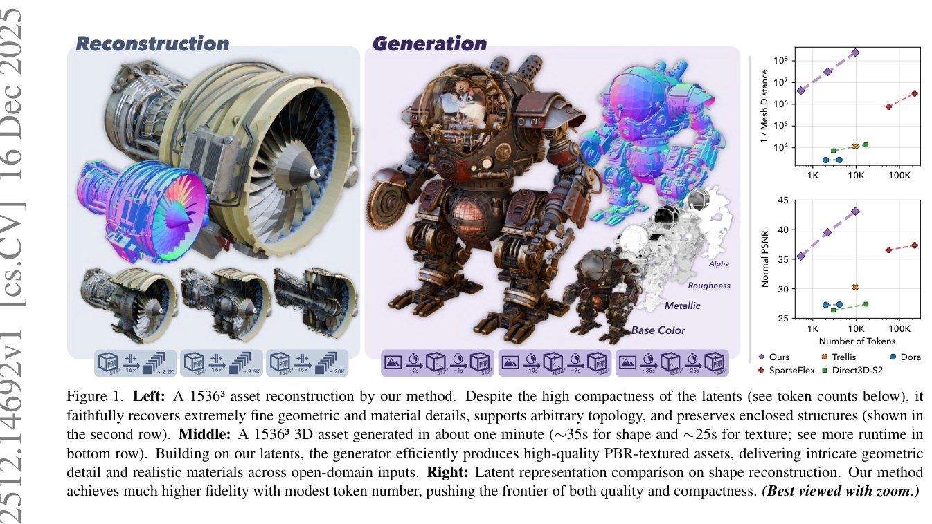
Figure 1. Left: A 1536³ asset reconstruction by our method. Despite the high compactness of the latents (see token counts below), it faithfully recovers extremely fine geometric and material details, supports arbitrary topology, and preserves enclosed structures (shown in the second row). Middle: A 1536³ 3D asset generated in about one minute (∼35s for shape and ∼25s for texture; see more runtime in bottom row). Building on our latents, the generator efficiently produces high-quality PBR-textured assets, delivering intricate geometric detail and realistic materials across open-domain inputs. Right: Latent representation comparison on shape reconstruction. Our method achieves much higher fidelity with modest token number, pushing the frontier of both quality and compactness. (Best viewed with zoom.)
图 1. 左:本方法对一张 资产的重建。尽管潜在表示高度紧凑(见下方标记数),仍能忠实恢复极为精细的几何与材质细节,支持任意拓扑,并保留封闭结构(见第二行)。中:约一分钟内生成的一张 三维资产(形状约 35 秒,纹理约 25 秒;更多运行时间见底行)。基于我们的潜在表示,生成器能高效产出高质量、带 PBR 纹理的资产,在开放域输入上给出细腻几何与真实材质。右:形状重建上的潜在表示比较。本方法以适中的标记数达到更高保真度,同时推进了质量与紧凑性的边界。(建议放大查看。)
Abstract
摘要
Recent advancements in 3D generative modeling have significantly improved the generation realism, yet the field is still hampered by existing representations, which struggle to capture assets with complex topologies and detailed appearance. This paper presents an approach for learning a structured latent representation from native 3D data to address this challenge. At its core is a new sparse voxel structure called O-Voxel, an omni-voxel representation that encodes both geometry and appearance. O-Voxel can robustly model arbitrary topology, including open, non-manifold, and fully-enclosed surfaces, while capturing comprehensive surface attributes beyond texture color, such as physically-based rendering parameters. Based on O-Voxel, we design a Sparse Compression VAE which provides a high spatial compression rate and a compact latent space. We train large-scale flow-matching models comprising 4B parameters for 3D generation using diverse public 3D asset datasets. Despite their scale, inference remains highly efficient. Meanwhile, the geometry and material quality of our generated assets far exceed those of existing models. We believe our approach offers a significant advancement in 3D generative modeling.
三维生成建模近来进步很快,生成结果的真实感已明显提高,但现有表示仍是瓶颈:复杂拓扑和细致外观往往难以同时稳住。本文提出一种从原生三维数据学习结构化潜在表示的方法,用以应对这一挑战。方法的核心是一种新的稀疏体素结构 O-Voxel,即同时编码几何与外观的全能体素(omni-voxel)表示。O-Voxel 能稳健地刻画任意拓扑,包括开放面、非流形以及完全封闭的表面,并能捕获超出纹理颜色的全面表面属性,例如物理渲染(PBR)参数。在 O-Voxel 之上,我们设计了稀疏压缩变分自编码器(Sparse Compression VAE,SC-VAE),它具有较高的空间压缩率,并能得到紧凑的潜在空间。我们利用多样的公开三维资产数据,训练总参数约 40 亿的大规模流匹配(flow-matching)模型,用于三维生成。尽管模型规模不小,推理仍然高效。与此同时,生成资产的几何和材质质量明显高于现有模型。我们认为,这一方法为三维生成建模带来了切实进展。
1 Introduction
1 引言
3D generative modeling has progressed at an unprecedented rate recently, spurred by innovations in latent 3D representation design and the integration of large latent learning and generative models [76, 65, 3, 21, 64]. These advancements have dramatically enhanced both reconstruction fidelity and generation realism, bringing 3D content creation closer to real-world deployment and industrial applications.
三维生成建模近来以前所未有的速度推进,这得益于潜在三维表示设计上的创新,以及大规模潜在学习与生成模型的引入 [76, 65, 3, 21, 64]。这些进展大幅提高了重建保真度和生成真实感,使三维内容创作更接近实际部署和工业应用。
Despite the progress, the field still lacks fundamental representations that can both faithfully capture the full-spectrum information of arbitrary 3D assets and effectively be processed into latents with neural networks. Recent large 3D generation models [76, 65, 6, 3, 64, 21, 34] predominantly leverage iso-surface fields (e.g., signed distance function, Flexicubes [53]) to represent geometry, which have intrinsic limitations in handling open surfaces, non-manifold geometry, and enclosed interior structures. Moreover, most existing works focus on 3D shape generation while neglecting the appearance and material information inherent in 3D assets that are fundamentally correlated with shape. [65] introduces a structured 3D latent (SLAT) representation that jointly models geometry and appearance, but its reliance on multiview 2D image feature input and pure rendering-based supervision leads to deficiencies in capturing complex structures and materials.
尽管已有进步,这一领域仍缺少能同时做到两件事的基础表示:既忠实捕获任意三维资产的全谱信息,又能有效地经神经网络处理成潜在变量。近来的大型三维生成模型 [76, 65, 6, 3, 64, 21, 34] 大多借助等值面场(例如符号距离函数、Flexicubes [53])来表示几何,而这类表示在处理开放面、非流形几何和封闭内部结构上有固有局限。此外,已有工作大多只关注三维形状生成,忽略了三维资产中与形状本质相关的外观与材质信息。[65] 提出了一种联合建模几何与外观的结构化三维潜在表示(SLAT),但它依赖多视图二维图像特征作为输入,并且只使用基于渲染的监督,因此在捕获复杂结构和材质时仍有不足。
In this work, we introduce a new “field-free” sparse voxel structure termed O-Voxel. O-Voxel is an omni-voxel representation that encodes both geometry and appearance, serving as a nexus between mesh assets and neural networks. The “omnipotence” of this structure not only lies in its integrated approach to modeling geometry and appearance but also in its robust capacity to handle their inherent complexity. For geometry, it can handle arbitrary topology including open, non-manifold, and fully-enclosed surfaces, unlike existing field-based methods. By introducing a flexible dual grid structure corresponding to the primal sparse voxels, it can accommodate complex topology without lossy data preprocessing and preserve sharp edge features and normal discontinuities for accurate geometry reproduction. For appearance, it can capture arbitrary surface attributes beyond mere texture color. In this work, we implement physically-based rendering (PBR) parameters aligned with surface geometry to enable re-lighting capability. In particular, it incorporates material opacity, allowing it to handle translucent surfaces—a capability not present in previous methods.
本文提出一种新的*“无场”稀疏体素结构,称为 O-Voxel。O-Voxel 是一种全能体素表示,同时编码几何与外观,在网格资产和神经网络之间充当中间枢纽。这一结构的“全能”不仅体现在把几何与外观放在同一套表示里,也体现在它能稳健地处理二者固有的复杂性。在几何上,它能处理包括开放面、非流形以及完全封闭表面在内的任意拓扑,这与现有基于场的方法不同。通过引入与原始稀疏体素相对应的灵活对偶网格(flexible dual grid),它可以在不做有损数据预处理的情况下容纳复杂拓扑,并保留锐利边缘特征和法向不连续,从而更准确地复现几何。在外观*上,它能捕获超出纹理颜色的任意表面属性。本文实现了与表面几何对齐的物理渲染(PBR)参数,以支持重新打光。特别地,它纳入了材料不透明度,因而能够表示半透明表面——这是先前方法所不具备的能力。
Another notable advantage of O-Voxel is its instant bidirectional conversions to and from raw 3D assets. The processes are both optimization-free and rendering-free. Transforming a mesh into this structure takes only a few seconds on a single CPU, while reconstructing surfaces and materials from it completes within tens of milliseconds.
O-Voxel 的另一个显著优点,是它与原始三维资产之间可以瞬时双向转换。这两个过程既不做优化,也不做渲染。把网格转换成该结构,在单颗 CPU 上只需数秒;从该结构重建表面和材质,则只需几十毫秒。
Given the O-Voxel representation, we design a sparse 3D variational autoencoder to learn a proper latent space. This leads to a native structured latent space compared to that in [65] which is built from multiview 2D information. Furthermore, we aim for a compact latent space to support efficient and high-resolution 3D generation. Utilizing a residual autoencoding design [2] applied to sparse voxel structure, our VAE achieves a 16 spatial downsampling, a high ratio not seen in prior voxel-based methods. Our approach encodes a fully textured asset with resolution into only 9.6K latent tokens with negligible perceptual degradation upon reconstruction. Experiments show that our reconstruction quality surpasses prior methods by a wide margin, albeit using substantially fewer tokens. In addition to enabling high-resolution 3D generation, our compact latent space also facilitates the scaling of the generative model.
有了 O-Voxel 表示后,我们设计稀疏三维变分自编码器,用以学习合适的潜在空间。由此得到的是原生结构化潜在空间,不同于 [65] 中由多视图二维信息搭建的潜在空间。我们还希望潜在空间足够紧凑,以支持高效、高分辨率的三维生成。把残差自编码设计 [2] 用到稀疏体素结构上,我们的 VAE 实现了 空间下采样,这一压缩比在先前基于体素的方法中未见。本方法可将一张完整带纹理、分辨率为 的资产编码为仅约 K 个潜在标记,重建时的感知损失可以忽略。实验表明,我们的重建质量大幅优于先前方法,所用标记数却明显更少。紧凑的潜在空间不仅使高分辨率三维生成成为可能,也便于把生成模型做大。
We train large flow-matching generative models in the learned latent space for image-to-3D generation. The models contain about 4 billion parameters in total and are trained on diverse public 3D asset datasets. Despite their scale, inference remains highly efficient: it takes only 3s for fully-textured assets generation, 17s for the resolution, and 60s for the resolution on a NVIDIA H100 GPU, which are significantly faster than existing large 3D generation models. Meanwhile, the geometry and material quality of our generated assets far exceed those of existing models, as demonstrated in our experiments. All our model, code, and dataset will be publicly released to facilitate reproduction and further research.
我们在学到的潜在空间中训练大规模流匹配生成模型,用于图像到三维生成。模型总参数约 40 亿,训练数据来自多样的公开三维资产库。尽管规模不小,推理仍然高效:在一块 NVIDIA H100 GPU 上,生成 全纹理资产约需 秒, 约需 秒, 约需 秒,明显快于现有大型三维生成模型。与此同时,生成资产的几何和材质质量也远超现有模型,实验部分将给出具体比较。模型、代码和数据集将全部公开,以便复现和后续研究。
2 Related Work
2 相关工作
3D Representations for Generation.
Effectively representing geometry and appearance for neural network processing is a key challenge in 3D generation. Early works adopted implicit fields or their discretized structures to represent shape, such as occupancy fields [41] and Signed Distance Functions (SDF) [48, 14, 22, 79]. NeRF [42, 59, 43] integrates geometry and appearance in a radiance field, yielding realistic rendering but suffering from low geometry quality and heavy sampling costs. Unstructured 3D representations, including meshes [45, 4], point clouds [46, 39, 81], and Gaussians [27, 72, 75, 20], offer explicit 3D representations but lack structural regularity, posing challenges for network processing and latent compression. Recent works have introduced structured representations tailored for 3D generation [21, 34]. They combine field-based iso-surface modeling with sparse voxels to achieve high-resolution geometry. However, their reliance on field-based primitives limits their capability to represent open or non-manifold surfaces and they do not handle appearance, unlike our approach.
面向生成的三维表示。
如何有效表示几何与外观,以便神经网络处理,是三维生成中的关键难题。早期工作用隐式场或其离散结构来表示形状,例如占据场 [41] 和符号距离函数(SDF) [48, 14, 22, 79]。NeRF [42, 59, 43] 在辐射场中同时表达几何与外观,渲染效果真实,但几何质量偏低,采样代价也高。非结构化三维表示,包括网格 [45, 4]、点云 [46, 39, 81] 和高斯 [27, 72, 75, 20],提供了显式三维表达,但缺少结构上的规整性,给网络处理和潜在压缩带来困难。近来有工作提出专为三维生成设计的结构化表示 [21, 34]。它们把基于场的等值面建模与稀疏体素结合起来,以实现高分辨率几何。不过,由于依赖基于场的基元,它们难以表示开放或非流形表面,也不处理外观,这与本方法不同。
Latent 3D Representations.
Recent advances in 3D generation have increasingly shifted from using explicit geometric representations to compact latent spaces, analogous to those used in the 2D domain [52]. Various latent formulations have been explored, including latent point clouds [30, 68, 6, 61], volumetric or hierarchical grids [47, 66, 51, 40], and triplane embeddings [63, 29, 19]. Among these, two latent paradigms have emerged as the dominant choices for recent large 3D generation models. The first is the unstructured latent, inspired by the Perceiver-style architectures [24], where 3D data are encoded as unordered feature vectors. Representative works include [74, 78] and the follow-up methods [26, 76, 31, 32, 23]. These methods can achieve strong compression but are typically constrained by reconstruction fidelity. The second category is the structured latent built upon sparsity priors, exemplified by [65] and its extensions [34, 21]. Such representations yield high geometric accuracy but require a larger number of latent tokens, which reduces compression efficiency. Some efforts [64, 5] attempted to mitigate this issue by optimizing network computation rather than improving latent compactness. In this work, our method learns a compact structured latent space directly from native 3D inputs, achieving higher spatial dowmsampling rate and fewer latent tokens.
潜在三维表示。
三维生成的近期进展,日益从使用显式几何表示转向紧凑潜在空间,这与二维领域的做法类似 [52]。人们探索过多种潜在形式,包括潜在点云 [30, 68, 6, 61]、体素或层次化网格 [47, 66, 51, 40],以及三平面嵌入 [63, 29, 19]。其中,有两种潜在范式成为近来大型三维生成模型的主要选择。第一种是受 Perceiver 风格架构 [24] 启发的非结构化潜在表示,把三维数据编码为无序特征向量。代表性工作包括 [74, 78] 及其后续方法 [26, 76, 31, 32, 23]。这类方法往往压缩能力强,但重建保真度通常受限。第二种是建立在稀疏先验之上的结构化潜在表示,以 [65] 及其扩展 [34, 21] 为代表。这类表示几何精度高,但需要更多潜在标记,压缩效率因而降低。有些工作 [64, 5] 试图通过优化网络计算来缓解这一问题,而不是提高潜在表示本身的紧凑性。本文的方法直接从原生三维输入学习紧凑的结构化潜在空间,空间下采样率更高,潜在标记也更少。
Large 3D Asset Generation Models and Systems.
With the rapid expansion of large-scale 3D asset datasets [13, 12, 77], there has been a surge in large models and systems capable of generating 3D assets with high-quality shapes and textures [76, 65, 6, 23, 69, 32, 33]. A common paradigm decomposes the generation into two stages: shape generation and multi-view texture synthesis [76, 23, 69, 32, 32, 33].
大型三维资产生成模型与系统。
随着大规模三维资产数据集迅速扩充 [13, 12, 77],能够生成高质量形状与纹理三维资产的大模型和系统大量出现 [76, 65, 6, 23, 69, 32, 33]。一种常见范式把生成拆成两个阶段:形状生成,以及多视图纹理合成 [76, 23, 69, 32, 32, 33]。

Figure 2: Overview of our approach. We introduce O-Voxel for shape and material representation (Sec. 3.1), based on which we employ Sparse Compression VAEs for compact latent space learning (Sec. 3.2) and large flow models for 3D generation (Sec. 3.3).
图 2:本方法总览。我们提出用于形状与材质表示的 O-Voxel(第 3.1 节),并在此基础上用稀疏压缩 VAE 学习紧凑潜在空间(第 3.2 节),再用大规模流模型做三维生成(第 3.3 节)。
While this pipeline benefits from powerful 2D image diffusion backbones, it typically requires complex multi-view rendering, baking, and texture alignment, which hinder scalability and often introduce appearance inconsistencies. [65] tackles 3D generation with material information, yet still relies on multiview baking to merge the generated mesh and 3D Gaussians for asset extraction. In contrast, our approach performs native, end-to-end 3D asset generation, directly producing high-fidelity, fully textured 3D assets without any view-dependent postprocessing.
这一流程可以借助强大的二维图像扩散骨干,但通常需要复杂的多视图渲染、烘焙和纹理对齐,既不利于扩展,也容易造成外观不一致。[65] 在三维生成中引入了材质信息,但提取资产时仍依赖多视图烘焙,把生成的网格与三维高斯合并。相比之下,本方法做的是原生、端到端的三维资产生成,直接产出高保真、完整带纹理的三维资产,无需任何依赖视角的后处理。
3 Method
3 方法
Our objective is to generate high-resolution 3D assets with arbitrary shape topology and flexible material attributes. An overview of our approach is presented in Fig. 2.
我们的目标,是生成具有任意形状拓扑和灵活材质属性的高分辨率三维资产。方法总览见图 2。
3.1 O-Voxel: A Native 3D Representation
3.1 O-Voxel:一种原生三维表示
Given a 3D asset, O-Voxel represents it as a collection of feature tuples associated with sparse voxels on a regular 3D grid of resolution :
给定一张三维资产,O-Voxel 把它表示为与稀疏体素相关联的特征元组集合;这些体素位于分辨率为 的规则三维网格上:
where encodes local geometric information, encodes material properties, and denotes the coordinate of the -th active voxel. Empty voxels that do not intersect with the asset are set inactive.
其中 编码局部几何信息, 编码材质属性, 表示第 个活跃体素的坐标。不与资产相交的空体素被设为非活跃。
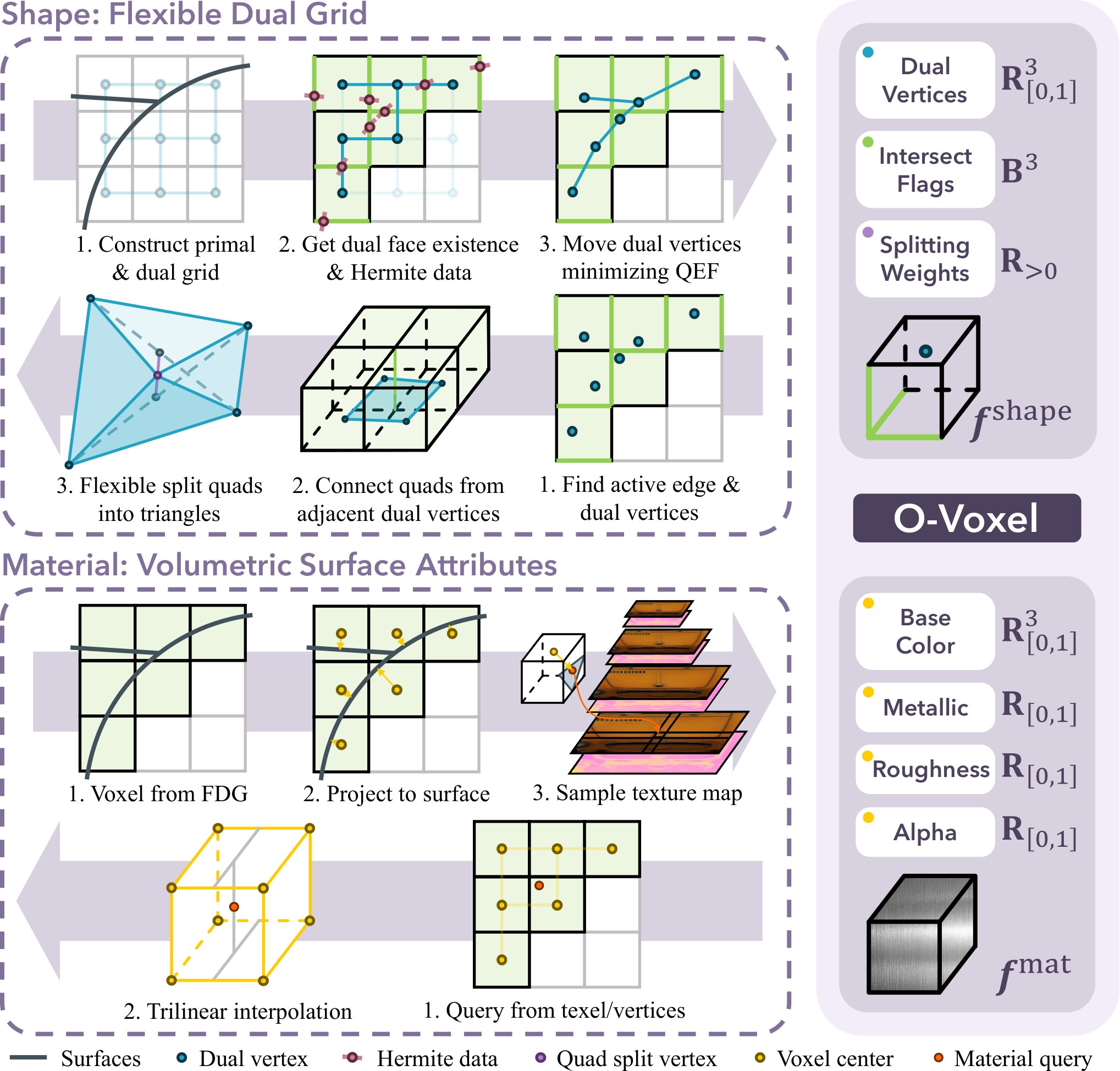
Figure 3: Illustration of O-Voxel and the instant bidirectional convertion between 3D asset and O-Voxel.
图 3:O-Voxel 示意,以及三维资产与 O-Voxel 之间的瞬时双向转换。
3.1.1 Flexible Dual Grid for Shape
The O-Voxel can robustly represent surfaces with arbitrary topology, owing to its Flexible Dual Grid formulation. In this dual grid, one vertex is defined per primal cell and one quadrilateral face per primal edge, connecting dual vertices in adjacent primal cells. By constructing a dual grid corresponding to the primal regular voxel grid, our algorithm flexibly adjusts the positions of dual vertices and the existence of dual grid faces to accurately represent arbitrary input surface data (illustrated in the first row of Fig. 3).
3.1.1 用于形状的灵活对偶网格
凭借灵活对偶网格表述,O-Voxel 能稳健地表示任意拓扑的表面。在这一对偶网格中,每个原始单元格定义一个顶点,每条原始棱定义一个四边形面,把相邻原始单元格中的对偶顶点连接起来。通过构造与原始规则体素网格相对应的对偶网格,算法可以灵活调整对偶顶点的位置以及对偶网格面是否存在,从而准确表示任意输入表面数据(见图 3 第一行)。
This formulation is inspired by Dual Contouring (DC) [25, 7], an algorithm to extract surfaces from a signed grid with edges tagged by Hermite data (i.e., intersection points and normals). The original DC was designed to process descritized scalar fields such as SDFs. Different from DC, we do not utilize any field representation. Our approach is straightforward: we directly use the asset’s mesh surface to determine edge intersection flags (rather than detecting sign changes as in DC) and to assign Hermite data. Each edge that intersects the mesh activates the corresponding dual face, and the associated Hermite data are then used to adjust the positions of the dual vertices. Given Hermite data , we compute the dual vertex in closed form using the following quadratic error function (QEF):
这一表述受到对偶等高线(Dual Contouring,DC) [25, 7] 的启发。DC 是一种从带有 Hermite 数据(即交点与法向)标记的有符号网格中提取表面的算法。原始 DC 是为处理离散化标量场(如 SDF)而设计的。与 DC 不同,我们不使用任何场表示。做法很直接:我们直接用资产的网格表面来确定边相交标志(而不是像 DC 那样检测符号变化),并据此指定 Hermite 数据。每条与网格相交的边会激活相应的对偶面,随后用相应的 Hermite 数据调整对偶顶点的位置。给定 Hermite 数据 ,我们用下面的二次误差函数(QEF)以闭式求出对偶顶点 :
The original QEF in DC only contains the first component, which measures the squared distance from to the plane determined by , . We introduce an additional error term that penalizes the distance between and any boundary edges of the mesh intersecting the primal cell, , as well as a regularization term that encourages to stay close to the average of the intersecting points, . The former guides the dual vertex to align with boundary edges, improving the representation of open surfaces, while the latter encourages a smoother vertex distribution and stabilizes the QEF optimization against singularities.
DC 中原来的 QEF 只包含第一项,它度量 到由 所确定平面的平方距离,。我们额外引入一项误差,惩罚 与任何穿过该原始单元格的网格边界棱之间的距离,;同时还加入一项正则,鼓励 靠近各交点的均值,。前者引导对偶顶点与边界棱对齐,从而更好地表示开放面;后者则促使顶点分布更平滑,并在出现奇异时稳住 QEF 优化。
Based on the above algorithm description, for each active voxel, our geometric feature comprises:
根据上述算法,对每个活跃体素,我们的几何特征 包括:
- • Dual vertex , a vertex within the grid to represent local surface shape.
- • 对偶顶点 ,网格内的一个顶点,用于表示局部表面形状。
- • Edge intersection flags , which determine the quad connections among neighboring dual vertices. We use the surface-edge intersections on 3 predefined voxel edges along the , , and axes, respectively (e.g., those that share the minimum-coordinate corner)[^1].
- • 边相交标志 ,用于决定相邻对偶顶点之间的四边形连接。我们分别使用沿 、、 轴预先指定的 3 条体素边上的表面–边交点(例如,共享最小坐标角点的那些边)[^1]。
- • Splitting weights , controlling how quadrilateral faces are adaptively subdivided into triangles, following the flexible topology rule in [53].
- • 剖分权重 ,控制如何把四边形面自适应地剖分成三角形,遵循 [53] 中的灵活拓扑规则。
The conversion algorithm between O-Voxel and mesh is summarized as follows (see also Fig. 3 for an illustration).
O-Voxel 与网格之间的转换算法可概括如下(示意见图 3)。
Mesh O-Voxel. Given a mesh, we first identify all voxel edges intersecting with the mesh surface and mark their neighboring voxels as active. The intersection points and their normals are computed analytically from mesh triangles, yielding Hermite data. The dual vertex for each active voxel is then calculated by solving the QEF in Eq. (2).
网格 O-Voxel。 给定一张网格,我们先找出所有与网格表面相交的体素边,并把它们的邻近体素标记为活跃。交点及其法向由网格三角形解析计算得到,从而得到 Hermite 数据。随后,通过求解式 (2) 中的 QEF,算出每个活跃体素的对偶顶点。
O-Voxel Mesh. From an O-Voxel, we recover mesh surfaces by connecting dual vertices across intersected edges, forming quadrilateral faces among neighboring active voxels. Each quadrilateral can be adaptively subdivided into two triangles guided by the splitting weights, allowing the surface to better conform to local geometric features.
O-Voxel 网格。 从 O-Voxel 恢复网格表面时,我们沿相交边连接对偶顶点,在相邻活跃体素之间形成四边形面。每个四边形可在剖分权重的引导下自适应地分成两个三角形,使表面更好地贴合局部几何特征。
The Flexible Dual Grid offers several key advantages:
灵活对偶网格有以下几项主要优点:
- Instant bidirectional conversion — it enables rapid mapping with meshes and supports high-resolution conversion with minimal computation overhead. The costly processes in prior works such as SDF evaluation, flood-fill procedure, and iterative optimization are not needed.
- 瞬时双向转换:它可以与网格快速互转,并以很小的计算开销支持高分辨率转换。先前工作中代价较高的过程,如 SDF 求值、泛洪填充以及迭代优化,都不必再做。
- Arability-topology modeling — it is free from the watertight and manifold constraints, enabling robust handling of arbitrary geometry including self-intersecting surfaces and fully-enclosed interior structures.
- 任意拓扑建模:它不受水密性和流形约束限制,能够稳健处理任意几何,包括自相交表面和完全封闭的内部结构。
- High precision and sharp feature preservation — the dual vertices are aligned with local geometric features by algorithm design [25], allowing for the preservation of sharp features. Additionally, the dual vertex positions and splitting weights can receive learnable adjustments by neural network using other supervisions such as rendering loss (see Section 3.2.2), further enhancing the flexibility and precision of the geometry.
- 高精度并保留锐利特征:对偶顶点按算法设计与局部几何特征对齐 [25],因而能够保留锐利特征。此外,对偶顶点位置和剖分权重还可以由神经网络依据渲染损失等其他监督做可学习调整(见第 3.2.2 节),进一步提高几何的灵活性和精度。
3.1.2 Volumetric Attributes for Material
The O-Voxel can model arbitrary surface attributes aligned with surface geometry, including color and other material attributes. In this work, we implement physically-based rendering (PBR) parameters to capture the intrinsic light–surface interaction characteristics of the materials. Specifically, our material feature for each active voxel consists of six channels:
3.1.2 用于材质的体属性
O-Voxel 可以建模与表面几何对齐的任意表面属性,包括颜色和其他材质属性。本文实现物理渲染(PBR)参数,以捕获材质固有的光–表面相互作用特性。具体而言,每个活跃体素的材质特征 包含六个通道:
where denotes the base color, the metallic ratio, the roughness, and the opacity. This parameterization follows the standard PBR convention widely adopted in modern physically-based rendering pipelines. The conversion between O-Voxel data and mesh texture is simple and fast, as illustrated in Fig. 3.
其中 表示基础色, 表示金属度, 表示粗糙度, 表示不透明度。这一参数化遵循现代物理渲染流程中广泛采用的标准 PBR 约定。O-Voxel 数据与网格纹理之间的转换简单而快速,如图 3 所示。
Texture O-Voxel. For an active voxel, we project its center onto each intersected triangle and sample each material attribute from the texture map using UV coordinates and appropriate mipmap levels. The sampled attributes are weighted-averaged based on the point-to-surface distances to obtain the final value. More details of this process can be found in the supplementary material.
纹理 O-Voxel。 对每个活跃体素,我们把它的中心投影到每张相交三角形上,再用 UV 坐标和适当的 mipmap 层级从纹理图中采样各材质属性。采样得到的属性按点到表面的距离做加权平均,得到最终取值。更多细节见补充材料。
O-Voxel Texture. During reconstruction, for each query point – either a mesh vertex position for vertex coloring or a 3D surface point corresponding to a texture map texel – material attributes are obtained via trilinear interpolation of the neighboring voxel attributes. The reconstructed mesh is then ready for rendering without need for any additional post-processing.
O-Voxel 纹理。 重建时,对每个查询点——既可以是用于顶点着色的网格顶点位置,也可以是对应纹理图纹素的三维表面点——材质属性通过对邻近体素属性做三线性插值得到。重建得到的网格即可直接用于渲染,无需任何额外后处理。
3.2 Sparse Compression VAE
3.2 稀疏压缩 VAE
We apply a VAE to learn a proper latent space from O-Voxel data. Our goal is to obtain a compact latent space that facilitates efficient, high-resolution 3D generation. We design a Sparse Compression VAE (SC-VAE) to achieve this.
我们用 VAE 从 O-Voxel 数据中学习合适的潜在空间。目标是得到一个紧凑的潜在空间,以便高效地做高分辨率三维生成。为此,我们设计了稀疏压缩变分自编码器(SC-VAE)。
3.2.1 Network Architecture
The architecture of our SC-VAE is illustrated in Fig. 4. Unlike transformer-based designs in priors work [65, 21], our SC-VAE employs a fully sparse-convolutional network that is both computationally efficient at high resolutions and generalizes well across scales. Following a U-shaped VAE design [52], our encoder hierarchically downsamples sparse voxel features through multiple residual blocks, and the decoder mirrors this process for reconstruction. We meticulously design the residual and (down/up)sampling blocks to enable high-compression encoding and faithful recovery.
3.2.1 网络结构
SC-VAE 的结构如图 4 所示。与先前工作中基于 Transformer 的设计 [65, 21] 不同,我们的 SC-VAE 采用完全稀疏卷积网络,在高分辨率下计算高效,并且跨尺度泛化良好。沿用 U 形 VAE 设计 [52],编码器通过多层残差块对稀疏体素特征做层次化下采样,解码器则镜像这一过程以完成重建。我们仔细设计了残差块以及下采样/上采样块,以实现高压缩编码和忠实恢复。
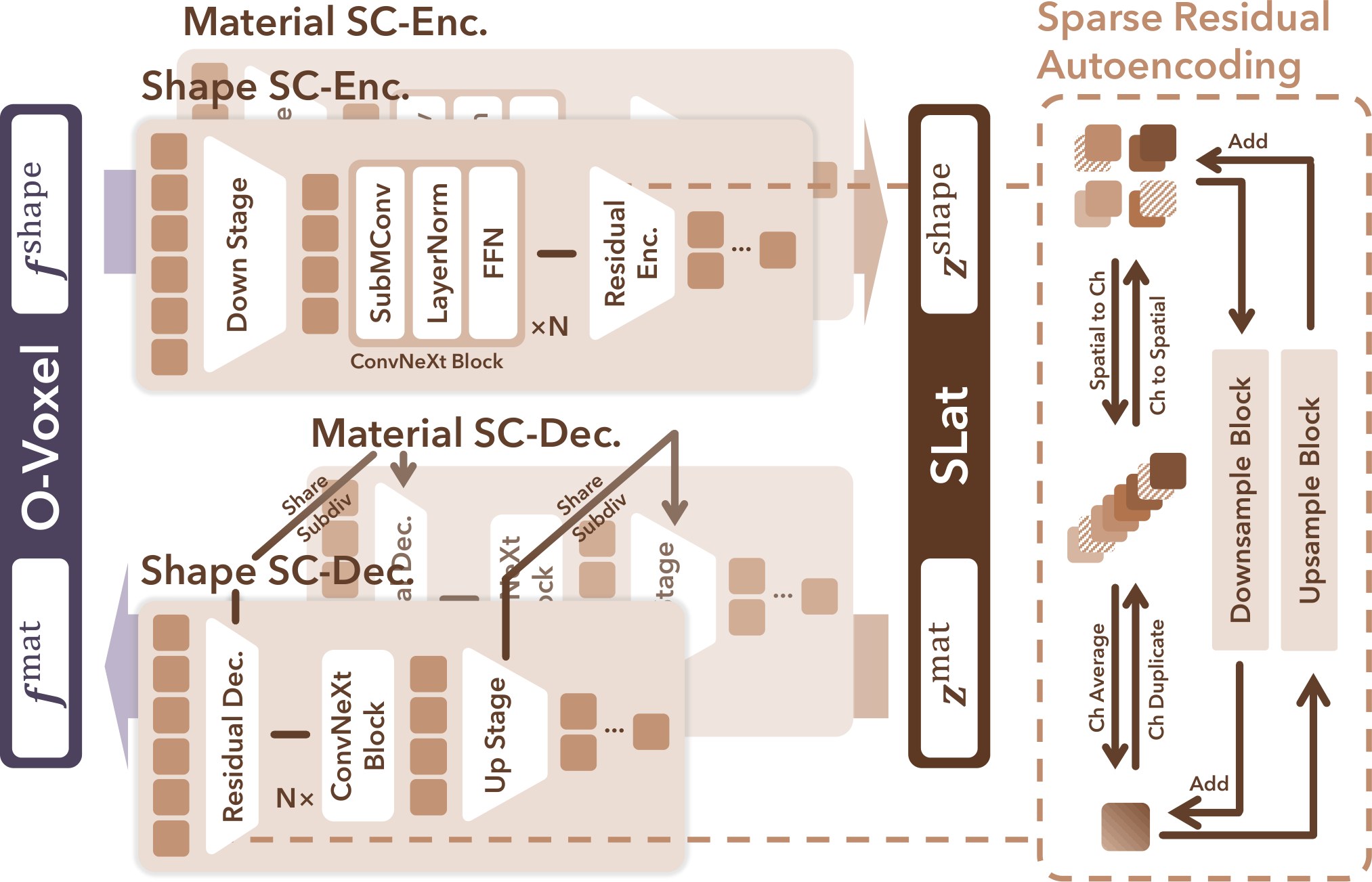
Figure 4: The network structure of SC-VAE.
图 4:SC-VAE 的网络结构。
Sparse Residual Autoencoding Layer.
We adapt the Residual Autoencoding principle from DC-AE [2] to sparse voxel data by introducing non-parametric residual shortcuts within downsampling and upsampling blocks. These shortcuts mitigate optimization challenges under high spatial compression by rearranging information between space and channel dimensions in the sparse grid.
稀疏残差自编码层。
我们把 DC-AE [2] 中的残差自编码原则改写到稀疏体素数据上,在下采样和上采样块中引入非参数残差捷径。这些捷径通过在稀疏网格的空间维与通道维之间重排信息,缓解高空间压缩下的优化困难。
Specifically, for a downsampling factor of 2, we aggregate each voxel’s eight children into its channel dimension. Given input features and target coarse features (typically ), we have:
具体而言,当下来样因子为 2 时,我们把每个体素的八个子体素聚合到其通道维。给定输入特征 和目标粗特征 (通常 ),有:
$$\begin{split}\quad F_{\text{coarse}}^{\text{raw}}&=\operatorname{stack}\big(F_{\text{child}{1}},\dots,F{\text{child}{8}}\big)\in\mathbb{R}^{8C},\
F{\text{coarse}}&=\operatorname{avg_groups}\big(F_{\text{coarse}}^{\text{raw}}\big)\in\mathbb{R}^{C^{\prime}},\end{split} \tag{4}$$
where the operation averages grouped channels to produce a coarse residual estimate. Missing voxels contribute zero vectors due to sparsity.
其中 操作对分组后的通道取平均,得到粗残差估计。由于稀疏性,缺失的体素贡献零向量。
During upsampling, a symmetric channel-to-space shortcut distributes each coarse feature back to its neighborhood:
在上采样时,一条对称的通道到空间捷径把每个粗特征再分配回其邻域:
$$\begin{split}\quad F_{\text{fine}}^{\text{raw}}&=\operatorname{unstack}\big(F_{\text{coarse}}\big)\in\mathbb{R}^{8C^{\prime}/8},\
F_{\text{fine}}&=\operatorname{dup_groups}\big(F_{\text{fine}}^{\text{raw}}\big)\in\mathbb{R}^{C},\end{split} \tag{5}$$
where copies channels within each group to match the target dimension.
其中 在每组内复制通道,以匹配目标维度。
Early-pruning Upsampler.
To further enhance efficiency, we employ an early-pruning mechanism [51] for the upsampler. Before each upsampling step, the module predicts a binary mask specifying the active child voxels of each parent node. Inactive nodes are skipped subsequently, thus greatly reducing runtime and memory cost.
提前剪枝上采样器。
为进一步提高效率,我们为上采样器采用提前剪枝机制 [51]。在每一步上采样之前,该模块预测一个二值掩码 ,标明每个父节点的活跃子体素。随后跳过非活跃节点,从而大幅降低运行时间和显存开销。
Optimized Residual Block.
Sparse convolutions exhibit low effective computation and parameter efficiency for high sparsity data. In light of this, we redesign the residual block by reducing convolutional layers and incorporating point-wise MLPs for richer feature transformation. Specifically, we substitute the standard design of two conv layers with a single conv layer and fewer normalization and activation layers, following the ConvNeXt-style [37] simplification. The second conv is replaced by a wide point-wise MLP – analogous to a Transformer FFN – which expands channel dimensions for enhanced nonlinearity and representation. This modification does not affect efficiency but improves reconstruction quality, as demonstrated in our experiments.
优化后的残差块。
在高度稀疏的数据上,稀疏卷积的有效计算量和参数效率都偏低。有鉴于此,我们重新设计残差块:减少卷积层,并引入逐点 MLP,以获得更丰富的特征变换。具体来说,我们把标准的两层卷积设计改成单层卷积,并减少归一化和激活层,沿用 ConvNeXt 风格 [37] 的简化。第二层卷积由一个较宽的逐点 MLP 代替——类似于 Transformer 中的 FFN——它扩展通道维,以增强非线性和表示能力。这一修改并不影响效率,却能提高重建质量,实验将给出验证。
3.2.2 VAE Training
SC-VAE is trained in two stages. In the first stage, we use low-resolution data to quickly stabilize learning with direct O-Voxel reconstruction loss and KL loss. For geometry features, Mean-Squared-Error (MSE) and Binary Cross Entropy (BCE) losses are applied on dual vertex positions and dual face flags , respectively. Material attributes and the pruning mask are supervised by the L1 and BCE loss, receptively:
3.2.2 VAE 训练
SC-VAE 分两阶段训练。第一阶段使用低分辨率数据,用直接的 O-Voxel 重建损失和 KL 损失迅速稳住学习。对几何特征,分别在对偶顶点位置 和对偶面标志 上使用均方误差(MSE)和二元交叉熵(BCE)损失。材质属性 和剪枝掩码 则分别用 L1 损失和 BCE 损失监督:
$$\begin{split}\mathcal{L}{\text{s1}}&=\lambda{\text{v}}|\hat{\boldsymbol{v}}-\boldsymbol{v}|{2}^{2}+\lambda{\delta}\operatorname{BCE}(\hat{\boldsymbol{\delta}},\boldsymbol{\delta})+\lambda_{\boldsymbol{\rho}}\operatorname{BCE}(\hat{\boldsymbol{\rho}},\boldsymbol{\rho})\
&+\lambda_{\text{mat}}|\hat{\boldsymbol{f}}^{\text{mat}}-\boldsymbol{f}^{\text{mat}}|{1}+\lambda{\text{KL}}\mathcal{L}_{\text{KL}}.\end{split} \tag{6}$$
In the second stage, we add rendering-based perceptual supervision at high resolution to enhance geometric and material fidelity. We render mask, depth, and normal maps and supervise them with L1 loss, augmented with SSIM and LPIPS terms on normals. The material attributes are rendered and supervised by these perceptual losses as well. The loss can be written as:
第二阶段,我们在高分辨率上加入基于渲染的感知监督,以增强几何和材质保真度。我们渲染掩码、深度和法向图,用 L1 损失监督,并在法向上附加 SSIM 和 LPIPS 项。材质属性同样被渲染,并由这些感知损失监督。损失可写为:
We randomly place cameras around with a shallow near plane to slice through the surface, encouraging the model to capture both external and internal structures. More details of the losses are provided in the supplementary material.
我们在周围随机放置相机,并采用较浅的近裁剪面,以便剖过表面,促使模型同时捕获外部和内部结构。损失的更多细节见补充材料。
To facilitate a sequential generation scheme for shape and material (in particular, to enable the application of material generation for given shapes), we learn decoupled latent spaces with two SC-VAEs: one models shape, while the other models material conditioned on the shape VAE’s subdivision structures during upsampling.
为便于对形状和材质采用顺序生成方案(尤其是为给定形状做材质生成),我们用两个 SC-VAE 学习解耦的潜在空间:一个建模形状,另一个在上采样时以形状 VAE 的剖分结构为条件来建模材质。
3.3 Generative Modeling
3.3 生成建模
Built upon the learned latent space, we construct a scalable generative framework following the overall design of [65]. We adopt full DiT-based architectures [49] trained with the flow matching paradigm [35] and extend the pipeline of [65] to fully leverage the power of our new latents.
在学到的潜在空间之上,我们沿用 [65] 的总体设计,构建可扩展的生成框架。我们采用完整的基于 DiT 的架构 [49],以流匹配范式 [35] 训练,并扩展 [65] 的流程,以充分发挥新潜在表示的能力。
Model and Generation Pipeline.
The complete generation process unfolds in three stages with three models: 1) sparse structure generation, which predicts the occupancy layout of the sparse voxel grid; 2) geometry generation, which produces geometry latents within active voxels; and 3) material generation, which synthesizes material latents aligned to the geometry structure. The first two stages largely follow the strategy of [65], forming the geometric backbone of the asset. The novel material generation stage models PBR materials directly in the native 3D space. A sparse DiT predicts material latents conditioned jointly on the input image and the generated geometry latents. This design unifies geometric and material generation in the same native 3D latent domain and ensures their spatially alignment under arbitrary topology.
模型与生成流程。
完整生成过程分三个阶段、对应三个模型:1)稀疏结构生成,预测稀疏体素网格的占据布局;2)几何生成,在活跃体素内产生几何潜在变量;3)材质生成,合成与几何结构对齐的材质潜在变量。前两个阶段大体沿用 [65] 的策略,构成资产的几何主干。新的材质生成阶段则直接在原生三维空间中建模 PBR 材质。一个稀疏 DiT 同时以输入图像和已生成的几何潜在变量为条件,预测材质潜在变量。这一设计把几何生成与材质生成统一在同一个原生三维潜在域中,并在任意拓扑下保证二者的空间对齐。
Architectural and Training Details.
All our DiT modules employ the AdaLN-single modulation [1] and Rotary Position Embedding (RoPE) [57] for better scalability and cross-resolution generalization. Image conditioning features are extracted from DINOv3-L [54]. Benefiting from the high spatial compression achieved by SC-VAE, our sparse DiTs discard the convolutional packing and skip connection designs in [65], resulting in a vanilla-style DiT which reduces complexity and improves efficiency.
结构与训练细节。
我们所有的 DiT 模块都采用 AdaLN-single 调制 [1] 和旋转位置编码(RoPE) [57],以便更好地扩展,并提高跨分辨率泛化能力。图像条件特征由 DINOv3-L [54] 提取。得益于 SC-VAE 实现的高空间压缩,我们的稀疏 DiT 不再使用 [65] 中的卷积打包和跳跃连接,从而得到更接近常规的 DiT,降低了复杂度,也提高了效率。
We first train the sparse structure generation with conditioning images to learn coarse occupancy priors and establish the global sparse layout. In the subsequent stages, training proceeds in a progressive manner, gradually increasing both the spatial and visual resolution. The geometry and material generators are scaled from outputs ( latent resolution) to outputs ( latent resolution), with the conditioning image resolution correspondingly increased to . This progressive strategy allows the learned priors to transfer smoothly across resolutions, enabling efficient training of large-scale sparse DiTs while maintaining fidelity in both geometry and material.
我们首先用 的条件图像训练稀疏结构生成,学习粗粒度占据先验,并确立全局稀疏布局。在后续阶段,训练以渐进方式进行,空间分辨率和视觉分辨率逐步提高。几何生成器和材质生成器从 输出(潜在分辨率 )扩展到 输出(潜在分辨率 ),条件图像分辨率相应地提高到 。这种渐进策略使已学到的先验能平稳迁移到不同分辨率,从而在保持几何与材质保真度的同时,高效训练大规模稀疏 DiT。
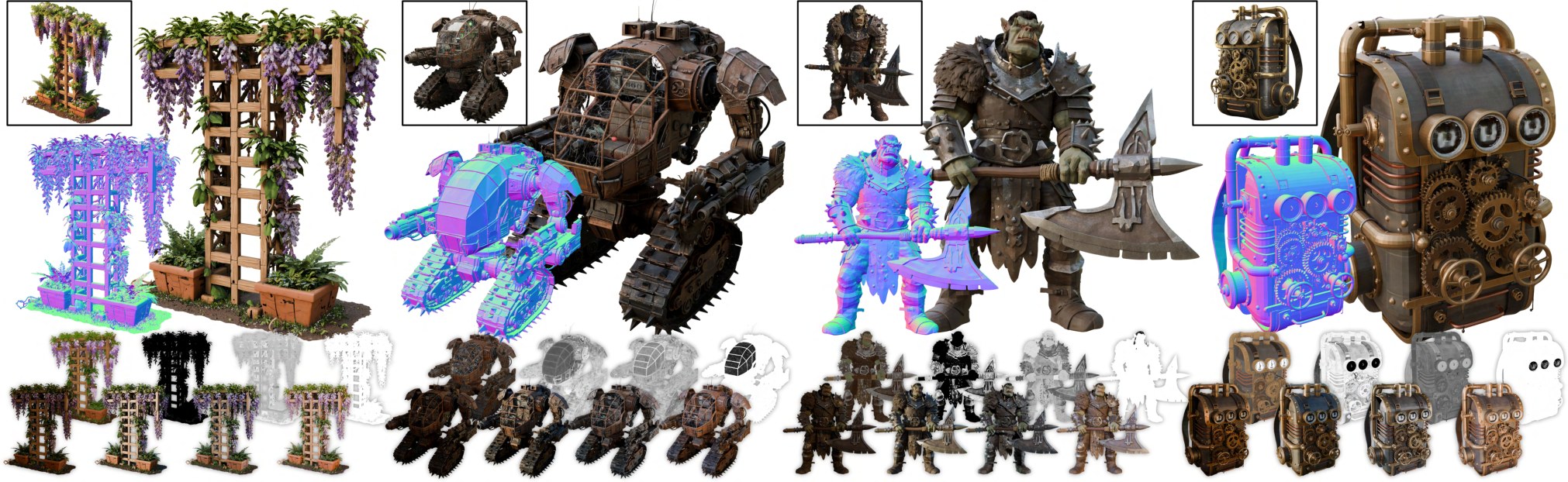
Figure 5: High-quality 3D assets generated by our method, featuring intricate geometric details and physically accurate materials with high visual fidelity, including thin structures, open surfaces, and translucent regions that highlight the model’s expressive capability.
图 5:本方法生成的高质量三维资产,具有细腻的几何细节和物理上准确、视觉保真度高的材质,包括薄结构、开放面和半透明区域,体现了模型的表达能力。
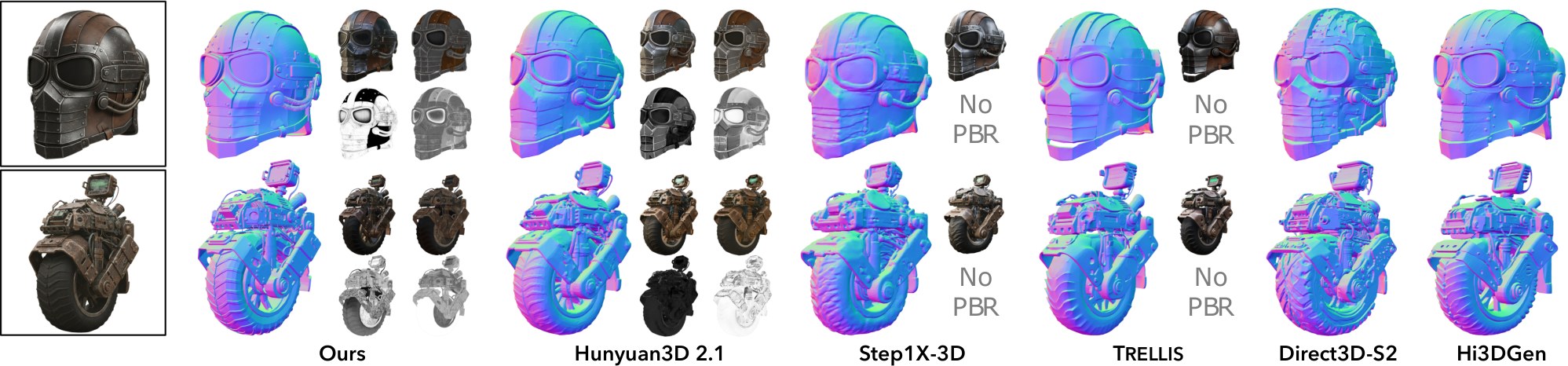
Figure 6: Visual comparison showing the normal (main image) and the final render, base color, metallic, and roughness (small images).
图 6:视觉比较。主图为法向,小图依次为最终渲染、基础色、金属度和粗糙度。
4 Experiments
4 实验
Implementation details.
Our SC-VAE is trained using the Trellis-500K setup [65] after filtering out assets without PBR materials, resulting in a curated collection from Objaverse-XL [12], ABO [9], and HSSD [28]. We use an optimized Triton [60] implementation for Submanifold convolution [18] to further improve training speed. SC-VAEs are trained on 16 H100 GPUs with a batch size of 128.
实现细节。
我们的 SC-VAE 按 Trellis-500K 的设置 [65] 训练,并过滤掉不含 PBR 材质的资产,最终整理自 Objaverse-XL [12]、ABO [9] 和 HSSD [28]。子流形卷积 [18] 使用优化后的 Triton [60] 实现,以进一步提高训练速度。SC-VAE 在 16 块 H100 GPU 上训练,批量大小为 128。
The generative model is trained on an extended collection of about 800K assets, augmented with TexVerse [77] to enrich PBR diversity and realism. For image prompts, we render 16 views per asset in Blender [10] with randomized FoVs and lighting. All models are trained using AdamW [38] (learning rate , weight decay ) with classifier-free guidance (drop rate ). Each DiT in our framework contains approximately 1.3B parameters (width: 1536, blocks: 30, heads: 12, MLP width: 8192), trained on 32 H100 GPUs with a batch size of 256.
生成模型在扩充后约 80 万张资产上训练,并加入 TexVerse [77],以丰富 PBR 的多样性和真实感。图像提示方面,我们在 Blender [10] 中为每张资产渲染 16 个视图,视场角和光照随机。所有模型均用 AdamW [38] 训练(学习率 ,权重衰减 ),并使用无分类器引导(丢弃率 )。框架中每个 DiT 约含 13 亿参数(宽度:1536,块数:30,头数:12,MLP 宽度:8192),在 32 块 H100 GPU 上训练,批量大小为 256。
For reconstruction evaluation, we use the Toys4K benchmark [56] together with a curated test set containing 90 assets featuring complex PBR materials and detailed shapes from recent Sketchfab assets [55] released within the past two years. Both test sets are unseen during training. For generation quality comparison and user studies, 100 AI-generated image prompts [16] are used to ensure training–testing disjointness. Split-sum renderer from nvdiffrec [44] is used for PBR asset rendering. All runtime statistics are reported on an NVIDIA A100 GPU. Additional details are provided in the supplementary material.
重建评测使用 Toys4K 基准 [56],以及一组精选测试集:其中包含 90 张来自近两年发布的 Sketchfab 资产 [55],具有复杂 PBR 材质和细致形状。两个测试集在训练中均未见过。生成质量比较和用户研究使用 100 张由 AI 生成的图像提示 [16],以保证训练与测试不相交。PBR 资产渲染使用 nvdiffrec [44] 的 split-sum 渲染器。全部运行时间均在一块 NVIDIA A100 GPU 上统计。更多细节见补充材料。
| Toys4K | Sketchfab Featured | |||||||||||||||
|---|---|---|---|---|---|---|---|---|---|---|---|---|---|---|---|---|
| Method | #Token (#Dim) | Dec. (s) | All Surface | Outer Surface | Normal | All Surface | Outer Surface | Normal | ||||||||
| MD | F11e-8 | CD | F11e-6 | PSNR | LPIPS | MD | F11e-8 | CD | F11e-6 | PSNR | LPIPS | |||||
| Dora | 2.0K | (131K) | – | 37.7 | 366.1 | 0.019 | 325.3 | 0.140 | 27.26 | 0.117 | 987.2 | 0.020 | 1182. | 0.130 | 22.02 | 0.175 |
| Dora | 4.1K | (262K) | – | 43.0 | 360.8 | 0.019 | 327.3 | 0.138 | 27.32 | 0.115 | 1139. | 0.020 | 1351. | 0.130 | 22.09 | 0.174 |
| Trellis | 9.6K | (77K) | 4 | 0.108 | 85.07 | 0.074 | 2.755 | 0.544 | 30.29 | 0.067 | 49.20 | 0.031 | 8.171 | 0.286 | 24.31 | 0.110 |
| Direct3D-S2 512 | 3.0K | (48K) | 8 | 1.86 | 137.6 | 0.002 | 23.85 | 0.027 | 26.34 | 0.138 | 128.0 | 0.002 | 26.64 | 0.032 | 22.76 | 0.159 |
| Direct3D-S2 1024 | 17K | (271K) | 8 | 13.0 | 73.17 | 0.001 | 13.45 | 0.001 | 27.38 | 0.134 | 70.13 | 0.001 | 14.06 | 0.000 | 23.82 | 0.138 |
| SparseFlex 512 | 56K | (452K) | 4 | 1.22 | 1.303 | 0.735 | 0.8366 | 0.840 | 36.56 | 0.027 | 3.221 | 0.487 | 1.881 | 0.783 | 29.46 | 0.055 |
| SparseFlex 1024 | 225K | (1799K) | 4 | 3.21 | 0.3132 | 0.845 | 0.8062 | 0.843 | 37.34 | 0.042 | 0.7593 | 0.684 | 1.129 | 0.828 | 32.12 | 0.036 |
| Ours 512 | 2.2K | (70K) | 16 | 0.077 | 0.0323 | 0.888 | 0.5890 | 0.851 | 39.54 | 0.013 | 0.1572 | 0.613 | 0.7447 | 0.833 | 31.00 | 0.034 |
| Ours 1024 | 9.6K | (306K) | 16 | 0.301 | 0.0042 | 0.971 | 0.5660 | 0.855 | 43.11 | 0.005 | 0.0170 | 0.868 | 0.6402 | 0.850 | 35.26 | 0.013 |
Table 1: Comparison of shape reconstruction efficiency and fidelity. MD and CD is reported ; runtime meaured on an A100 GPU.
| Toys4K | Sketchfab Featured | |||||||||||||||
|---|---|---|---|---|---|---|---|---|---|---|---|---|---|---|---|---|
| 方法 | 标记数(维度) | 解码(秒) | 全部表面 | 外表面 | 法向 | 全部表面 | 外表面 | 法向 | ||||||||
| MD | F11e-8 | CD | F11e-6 | PSNR | LPIPS | MD | F11e-8 | CD | F11e-6 | PSNR | LPIPS | |||||
| Dora | 2.0K | (131K) | – | 37.7 | 366.1 | 0.019 | 325.3 | 0.140 | 27.26 | 0.117 | 987.2 | 0.020 | 1182. | 0.130 | 22.02 | 0.175 |
| Dora | 4.1K | (262K) | – | 43.0 | 360.8 | 0.019 | 327.3 | 0.138 | 27.32 | 0.115 | 1139. | 0.020 | 1351. | 0.130 | 22.09 | 0.174 |
| Trellis | 9.6K | (77K) | 4 | 0.108 | 85.07 | 0.074 | 2.755 | 0.544 | 30.29 | 0.067 | 49.20 | 0.031 | 8.171 | 0.286 | 24.31 | 0.110 |
| Direct3D-S2 512 | 3.0K | (48K) | 8 | 1.86 | 137.6 | 0.002 | 23.85 | 0.027 | 26.34 | 0.138 | 128.0 | 0.002 | 26.64 | 0.032 | 22.76 | 0.159 |
| Direct3D-S2 1024 | 17K | (271K) | 8 | 13.0 | 73.17 | 0.001 | 13.45 | 0.001 | 27.38 | 0.134 | 70.13 | 0.001 | 14.06 | 0.000 | 23.82 | 0.138 |
| SparseFlex 512 | 56K | (452K) | 4 | 1.22 | 1.303 | 0.735 | 0.8366 | 0.840 | 36.56 | 0.027 | 3.221 | 0.487 | 1.881 | 0.783 | 29.46 | 0.055 |
| SparseFlex 1024 | 225K | (1799K) | 4 | 3.21 | 0.3132 | 0.845 | 0.8062 | 0.843 | 37.34 | 0.042 | 0.7593 | 0.684 | 1.129 | 0.828 | 32.12 | 0.036 |
| 本文 512 | 2.2K | (70K) | 16 | 0.077 | 0.0323 | 0.888 | 0.5890 | 0.851 | 39.54 | 0.013 | 0.1572 | 0.613 | 0.7447 | 0.833 | 31.00 | 0.034 |
| 本文 1024 | 9.6K | (306K) | 16 | 0.301 | 0.0042 | 0.971 | 0.5660 | 0.855 | 43.11 | 0.005 | 0.0170 | 0.868 | 0.6402 | 0.850 | 35.26 | 0.013 |
表 1:形状重建效率与保真度的比较。MD 与 CD 以 报告;运行时间在一块 A100 GPU 上测量。
4.1 3D Asset Reconstruction
4.1 三维资产重建
Shape Reconstruction.
We compare with four representative baselines: Dora [3] based on Shape2Vecset; Trellis [65], Direct3D-s2 [64], and SparseFlex [21] based on sparse voxel structure. For evaluation, we employ multiple metrics: (i) Mesh Distance (MD) calculated as Bidirectional Point-to-Mesh Distance with F1-score to measure reconstruction fidelity of meshes including internal structures; (ii) Chamfer Distance with F1-score computed on point clouds sampled from visible surfaces, focusing only on external shapes; and (iii) surface quality metrics using PSNR and LPIPS of rendered normal maps.
形状重建。
我们与四个有代表性的基线比较:基于 Shape2Vecset 的 Dora [3],以及基于稀疏体素结构的 Trellis [65]、Direct3D-s2 [64] 和 SparseFlex [21]。评测采用多项指标:(i)网格距离(Mesh Distance,MD),按双向点到网格距离计算,并配以 F1 分数,用于衡量包含内部结构在内的网格重建保真度;(ii)在从可见表面采样的点云上计算 Chamfer 距离及相应 F1 分数,只关注外部形状;(iii)用渲染法向图的 PSNR 和 LPIPS 作为表面质量指标。
As shown in Table 1, our method consistently outperforms all baselines by a substantial margin across every metric, despite using only a modest number of tokens and requiring significantly less runtime. This demonstrates not only its superior geometric fidelity, finer detail preservation, and more accurate modeling of internal structures, but also the high efficiency of our approach.
如表 1 所示,本方法在每一项指标上都大幅优于所有基线,所用标记数却并不多,运行时间也明显更短。这说明它不仅几何保真度更高、细节保留更好、内部结构建模更准确,方法本身也更高效。
Material Reconstruction.
As no suitable baseline exists for encoding only material properties given shapes, we report metrics solely for our method. We assess the fidelity of directly rendered PBR attribute maps and shaded images using PSNR and LPIPS. Our method achieves 38.89 dB / 0.033 on PBR attributes and 38.69 dB / 0.026 on shaded images, demonstrating faithful material reproduction and consistent geometry–appearance alignment.
材质重建。
由于不存在适合的基线,可在给定形状下只编码材质属性,我们仅报告本方法的指标。我们用 PSNR 和 LPIPS 评估直接渲染的 PBR 属性图以及着色图像的保真度。本方法在 PBR 属性上达到 38.89 dB / 0.033,在着色图像上达到 38.69 dB / 0.026,表明材质复现忠实,几何与外观对齐一致。
| Method | Alignment | Quality (User Study) | ||||
|---|---|---|---|---|---|---|
| CLIP | CLIP-N | ULIP-2 | Uni3D | Pref% | Pref-N% | |
| Trellis | 0.876 | 0.748 | 0.470 | 0.414 | 6.40% | 2.82% |
| Hi3DGen | – | 0.753 | 0.395 | 0.373 | – | 6.57% |
| Direct3D-S2 | – | 0.746 | 0.420 | 0.392 | – | 12.2% |
| Step1X-3D | 0.875 | 0.738 | 0.464 | 0.411 | 11.8% | 0.469% |
| Hunyuan3D 2.1 | 0.869 | 0.753 | 0.474 | 0.427 | 13.3% | 7.51% |
| Ours | 0.894 | 0.758 | 0.477 | 0.436 | 66.5% | 69.0% |
Table 2: Comparison of image-to-3D generation results. -N: measured with normal map.
| 方法 | 对齐 | 质量(用户研究) | ||||
|---|---|---|---|---|---|---|
| CLIP | CLIP-N | ULIP-2 | Uni3D | 偏好% | 偏好-N% | |
| Trellis | 0.876 | 0.748 | 0.470 | 0.414 | 6.40% | 2.82% |
| Hi3DGen | – | 0.753 | 0.395 | 0.373 | – | 6.57% |
| Direct3D-S2 | – | 0.746 | 0.420 | 0.392 | – | 12.2% |
| Step1X-3D | 0.875 | 0.738 | 0.464 | 0.411 | 11.8% | 0.469% |
| Hunyuan3D 2.1 | 0.869 | 0.753 | 0.474 | 0.427 | 13.3% | 7.51% |
| 本文 | 0.894 | 0.758 | 0.477 | 0.436 | 66.5% | 69.0% |
表 2:图像到三维生成结果的比较。-N:用法向图测量。
4.2 Image to 3D Generation
4.2 图像到三维生成
We next evaluate the generative capabilities of our framework by producing 3D assets conditioned on input images. Fig. 5 presents representative results, illustrating both geometric fidelity and material realism.
接下来,我们以输入图像为条件生成三维资产,评估框架的生成能力。图 5 给出代表性结果,同时展示几何保真度与材质真实感。
Leveraging the compact latent space compressing O-Voxels, our method generates assets that faithfully preserve fine-scale structures, sharp surface features, and internally complex or non-manifold shapes—ranging from detailed gears, enclosed cockpit and open leaves and flowers. It also reproduces vivid, realistic PBR textures with physically consistent shading under novel lighting, including challenging translucent or reflective materials such as glass and metal. Together, These results demonstrate that our native 3D latent space enables the generation of tightly aligned, high-fidelity geometry and photorealistic appearance, even for topologically complex assets.
借助对 O-Voxel 做压缩后得到的紧凑潜在空间,本方法生成的资产能忠实保留细尺度结构、锐利表面特征,以及内部复杂或非流形的形状——从精细的齿轮、封闭座舱,到开放的叶片与花朵。它也能复现鲜明、真实的 PBR 纹理,并在新光照下给出物理上一致的着色,包括玻璃和金属等具有挑战性的半透明或反射材质。这些结果一并表明,我们的原生三维潜在空间能够生成紧密对齐、高保真的几何和照片级外观,即便资产在拓扑上很复杂。
Qualitative comparison.
We compare our approach against state-of-the-art 3D generation systems, including Trellis [65], Hi3DGen [70], Direct3D-s2 [64], Step1X-3D [32], and Hunyuan3D 2.1 [23]. Samples from Fig. 6 demonstrate that our method achieves superior generation quality—delivering accurate and detailed geometry, physically plausible materials, and faithful prompt alignment.
定性比较。
我们与当前先进的三维生成系统比较,包括 Trellis [65]、Hi3DGen [70]、Direct3D-s2 [64]、Step1X-3D [32] 和 Hunyuan3D 2.1 [23]。图 6 中的样本表明,本方法的生成质量更高:几何准确而细致,材质在物理上合理,并且与提示对齐得更好。
Quantitative comparison.
We conduct quantitative evaluation using AI-generated images. Visual alignment is measured with the CLIP score [50], while multimodal models ULIP-2 [67] and Uni3D [80] are employed to assess the geometric similarity. Table 2 shows that our method achieves the highest alignment score across all metrics, demonstrating clear superiority in visual and geometric consistency.
定量比较。
我们用 AI 生成的图像做定量评测。视觉对齐用 CLIP 分数 [50] 衡量,几何相似性则用多模态模型 ULIP-2 [67] 和 Uni3D [80] 评估。表 2 显示,本方法在全部对齐指标上都取得最高分,视觉与几何一致性明显更好。
We also conduct a user study with about 40 participants to evaluate perceptual quality. Using 100 AI-generated image prompts, we generate assets with each method under identical conditions without curation and collect preference votes. Table 2 shows our method is favored by participants, highlighting its clear superiority in visual realism, richness of geometric detail, and alignment with input prompts.
我们还组织了约 40 名参与者的用户研究,以评估感知质量。使用 100 张 AI 生成的图像提示,在相同条件下、不做挑选地用各方法生成资产,并收集偏好投票。表 2 显示,参与者更偏好本方法,说明它在视觉真实感、几何细节丰富程度以及与输入提示的对齐上具有明显优势。
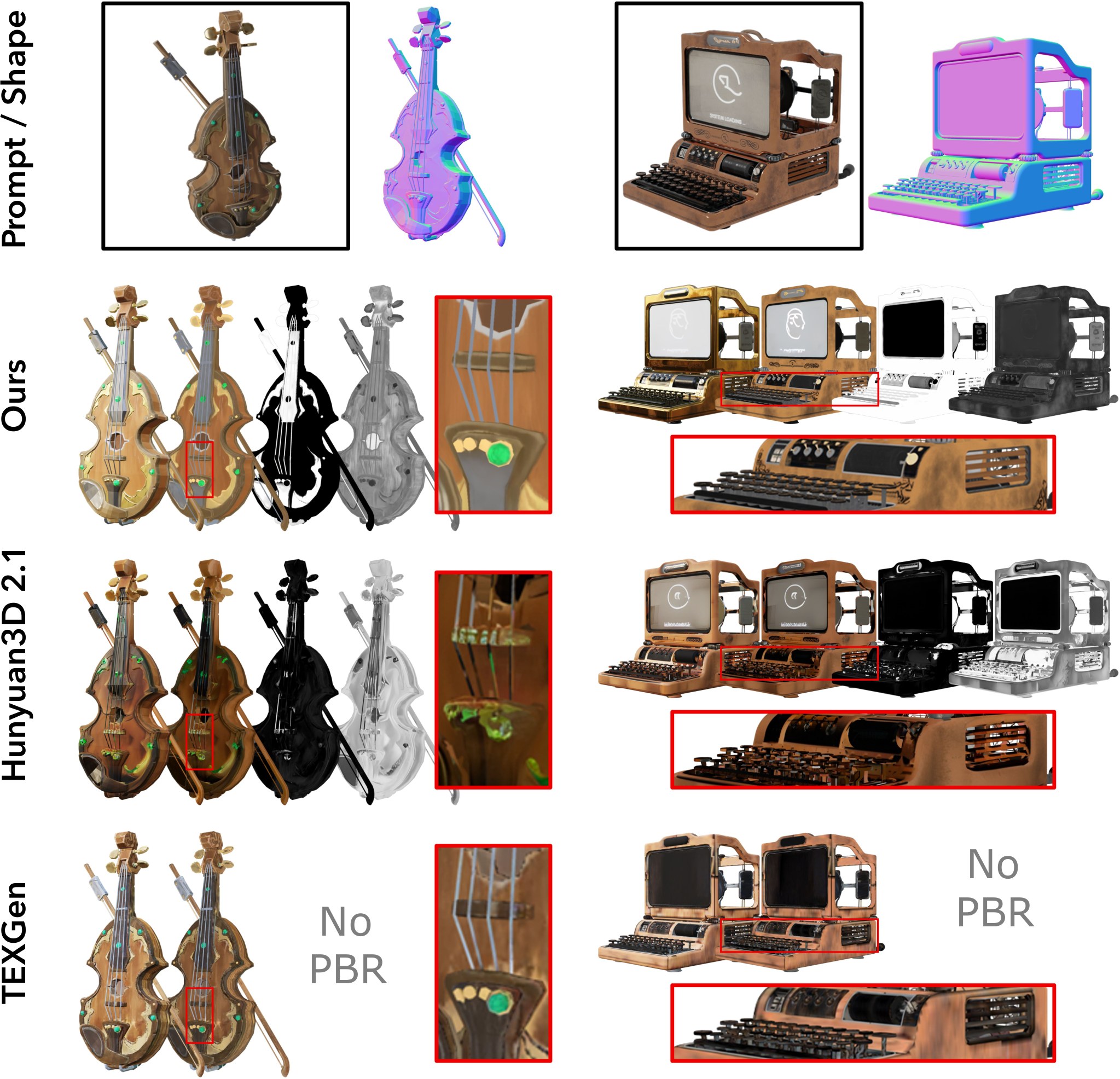
Figure 7: Visual comparison of PBR texture generation.
图 7:PBR 纹理生成的视觉比较。
4.3 Shape-Conditioned Texture Generation
4.3 形状条件下的纹理生成
The third stage of our generation pipeline can be independently used as a 3D PBR texture synthesis model given 3D mesh and reference image. To evaluate its performance, we compare against representative baselines: multi-view PBR generation and fusion methods Hunyuan3D-Paint [23], and UV-based TEXGen [71].
生成流程的第三阶段可以独立用作三维 PBR 纹理合成模型,输入为三维网格和参考图像。为评估其表现,我们与有代表性的基线比较:多视图 PBR 生成与融合方法 Hunyuan3D-Paint [23],以及基于 UV 的 TEXGen [71]。
As shown in Fig. 7, multi-view approaches often suffer from inconsistencies both between the shape and synthesized images, as well as across different views, resulting in ghosting or blurred textures. UV-based methods suffer from ambiguous UV charts and seam artifacts, resulting in degraded visual quality. In contrast, our framework performs appearance reasoning natively in 3D. This enables sharper textures, consistent shape–material alignment, and synthesis of textures for internal surfaces, crucial for complex assets with occluded or non-manifold geometry.
如图 7 所示,多视图方法往往既在形状与合成图像之间不一致,也在不同视图之间不一致,从而出现重影或模糊纹理。基于 UV 的方法则受困于含混的 UV 图表和接缝伪影,视觉质量下降。相比之下,我们的框架在原生三维空间中做外观推理。这能得到更锐利的纹理、更一致的形状–材质对齐,并能合成内部表面的纹理,这对带有遮挡或非流形几何的复杂资产尤为重要。
4.4 Ablation and Design Analysis
4.4 消融与设计分析
We conduct ablation study to analyze the architecture design of SC-VAE. All ablations are conducted on the curated sketchfab assets at a resolution of .
我们对 SC-VAE 的结构设计做消融研究。全部消融都在精选的 Sketchfab 资产上进行,分辨率为 。
| Setting | #Token | Dec. (ms) | MD | F11e-8 | PSNR | LPIPS |
|---|---|---|---|---|---|---|
| SC-VAE f16c32 | 503 | 28.6 | 1.032 | 0.312 | 27.26 | 0.072 |
| w/o Residual AE | 503 | 28.7 | 1.747 | 0.268 | 26.73 | 0.081 |
| w/o Opt. ResBlock | 503 | 29.6 | 1.198 | 0.285 | 26.67 | 0.083 |
| SC-VAE f32c128 | 118 | 33.9 | 1.405 | 0.273 | 26.65 | 0.081 |
| w/o Residual AE | 118 | 34.0 | 7.394 | 0.192 | 25.01 | 0.102 |
Table 3: Ablation study of SC-VAE architecture designs.
| 设置 | 标记数 | 解码(毫秒) | MD | F11e-8 | PSNR | LPIPS |
|---|---|---|---|---|---|---|
| SC-VAE f16c32 | 503 | 28.6 | 1.032 | 0.312 | 27.26 | 0.072 |
| 去掉残差自编码 | 503 | 28.7 | 1.747 | 0.268 | 26.73 | 0.081 |
| 去掉优化残差块 | 503 | 29.6 | 1.198 | 0.285 | 26.67 | 0.083 |
| SC-VAE f32c128 | 118 | 33.9 | 1.405 | 0.273 | 26.65 | 0.081 |
| 去掉残差自编码 | 118 | 34.0 | 7.394 | 0.192 | 25.01 | 0.102 |
表 3:SC-VAE 结构设计的消融研究。
Sparse residual autoencoding.
To evaluate the effect of the sparse residual autoencoding layer, we compare SC-VAE with a baseline using average pooling and nearest-neighbor upsampling. As shown in Table 3, the baseline exhibits severe quality degradation: MD increases by 69% and PSNR decreases 0.5dB at compression, worsening to 526% and 1.6dB at . In contrast, the sparse residual design maintains high fidelity across compression ratios, confirming its robustness under strong spatial bottlenecks.
稀疏残差自编码。
为评估稀疏残差自编码层的作用,我们将 SC-VAE 与使用平均池化和最近邻上采样的基线比较。如表 3 所示,该基线质量明显下降:在 压缩时,MD 上升 69%,PSNR 下降 0.5 dB;在 时进一步恶化到 526% 和 1.6 dB。相比之下,稀疏残差设计在不同压缩比下都能保持高保真度,说明它在较强的空间瓶颈下仍然稳健。
Optimized residual block.
To assess the effect of the optimized residual block, we compare SC-VAE with a baseline using standard residual blocks. Table 3 shows that this leads to a clear drop in reconstruction quality, MD increases by 16% and PSNR decreases by 0.6dB, while runtime remains unchanged. This confirms that the hybrid sparse convolution and point-wise MLP design better preserves fine-scale details without sacrificing efficiency.
优化后的残差块。
为评估优化残差块的作用,我们将 SC-VAE 与使用标准残差块的基线比较。表 3 显示,重建质量明显下降:MD 上升 16%,PSNR 下降 0.6 dB,运行时间则基本不变。这说明,稀疏卷积与逐点 MLP 的混合设计能在不牺牲效率的前提下,更好地保留细尺度细节。
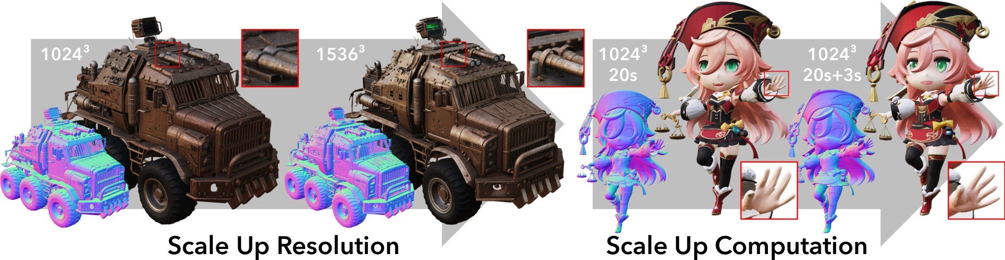
Figure 8: Scaling up resolution for finer detail and compute for higher quality during test time. (Best viewed with zoom)
图 8:测试时提高分辨率以获得更细细节,并增加计算量以提高质量。(建议放大查看)
4.5 Test-time Compute and Resolution Scaling
4.5 测试时的计算量与分辨率扩展
Our framework enables flexible test-time scaling of both compute and resolution, facilitated by the efficiency of our compact latent space. Notably, our generation process requires significantly fewer tokens than prior approaches, thanks to SC-VAE’s spatial compression. This efficiency permits a cascaded application of the second-stage generator, allowing for the synthesis of shapes at resolutions exceeding the training scale efficiently. Specifically, after predicting the O-Voxel structure from the gemetry latent, we can downsample it into a higher-res sparse structure layout (e.g., max-pooling a generated O-Voxel to a sparse structure resolution). Subsequently, we re-apply the geometry generation stage to obtain a higher-res shape (a sparse structure to a O-Voxel). See Fig. 8 (left) for an exmaple.
得益于紧凑潜在空间的效率,我们的框架可以在测试时灵活扩展计算量和分辨率。值得注意的是,由于 SC-VAE 具有 空间压缩,本方法的生成过程所需标记数明显少于先前方法。这一效率使第二阶段生成器可以级联使用,从而高效地在超过训练尺度的分辨率上合成形状。具体而言,从几何潜在变量预测出 O-Voxel 结构后,我们可以把它下采样为更高分辨率的稀疏结构布局(例如,对生成的 O-Voxel 做最大池化,得到 的稀疏结构分辨率)。随后再次运行几何生成阶段,得到更高分辨率的形状(从 稀疏结构得到 O-Voxel)。示例见图 8(左)。
Similar stratgies can be applied when operating within the trained resolution to improve generation quality. Rather than directly using the sparse structure generated by the first stage, one can obtain an alternative by downsampling a generated O-Voxel (e.g., downsampling a O-Voxel to a sparse structure). This can correct local errors and yield cleaner layouts for the subsequent high-resolution generation (e.g., a O-Voxel). Such a cascaded inference mechanism offers a controllable trade-off between computational efficiency and generation quality. As demonstrated in Fig. 8 (right), cascaded inference yielded finer details and enhanced structural stability.
在训练分辨率之内操作时,也可以采用类似策略来提高生成质量。不必直接使用第一阶段生成的稀疏结构,而可以对已生成的 O-Voxel 做下采样,得到另一种布局(例如,把 O-Voxel 下采样为 稀疏结构)。这可以修正局部错误,并为后续的高分辨率生成(例如 O-Voxel)提供更干净的布局。这种级联推理机制,在计算效率与生成质量之间提供了可控的权衡。如图 8(右)所示,级联推理带来了更细的细节,结构也更稳定。
5 Conclusion
5 结论
We present an approach for learning a comprehensive yet compact structured 3D latent representation for 3D generation. A key innovation is O-Voxel, an omni-voxel representation that is capable of encoding complex geometry and materials. We also introduce a Sparse Compression VAE that achieves a high spatial compression rate on O-Voxel to construct the latent space. Our large flow-matching models deliver substantially superior generation quality compared to existing methods while maintaining high efficiency. We believe our approach offers a significant advancement in 3D generative modeling, enhancing both the efficiency and realism of 3D content creation and opening avenues for broader applications across various domains.
我们提出一种学习全面而又紧凑的结构化三维潜在表示的方法,用于三维生成。一项关键创新是 O-Voxel,一种能够编码复杂几何与材质的全能体素表示。我们还引入稀疏压缩 VAE,对 O-Voxel 实现较高的空间压缩率,并据此构建潜在空间。大规模流匹配模型在保持高效率的同时,生成质量显著优于现有方法。我们认为,这一方法为三维生成建模带来了切实进展,既提高了三维内容创作的效率和真实感,也为更广泛的应用打开了空间。
References
参考文献
[1] J. Chen, Y. Jincheng, G. Chongjian, L. Yao, E. Xie, Z. Wang, J. Kwok, P. Luo, H. Lu, and Z. Li (2024) PixArt- α \alpha : fast training of diffusion transformer for photorealistic text-to-image synthesis . In ICLR , Cited by: 1st item , §3.3 .
[2] J. Chen, H. Cai, J. Chen, E. Xie, S. Yang, H. Tang, M. Li, Y. Lu, and S. Han (2024) Deep compression autoencoder for efficient high-resolution diffusion models . arXiv preprint arXiv:2410.10733 . Cited by: §A.2 , §1 , §3.2.1 .
[3] R. Chen, J. Zhang, Y. Liang, G. Luo, W. Li, J. Liu, X. Li, X. Long, J. Feng, and P. Tan (2025) Dora: sampling and benchmarking for 3d shape variational auto-encoders . In Proceedings of the Computer Vision and Pattern Recognition Conference , pp. 16251–16261 . Cited by: §1 , §1 , §4.1 .
[4] Y. Chen, T. He, D. Huang, W. Ye, S. Chen, J. Tang, X. Chen, Z. Cai, L. Yang, G. Yu, et al. (2024) MeshAnything: artist-created mesh generation with autoregressive transformers . arXiv preprint arXiv:2406.10163 . Cited by: §2 .
[5] Y. Chen, Z. Li, Y. Wang, H. Zhang, Q. Li, C. Zhang, and G. Lin (2025) Ultra3d: efficient and high-fidelity 3d generation with part attention . arXiv preprint arXiv:2507.17745 . Cited by: §2 .
[6] Z. Chen, J. Tang, Y. Dong, Z. Cao, F. Hong, Y. Lan, T. Wang, H. Xie, T. Wu, S. Saito, et al. (2024) 3DTopia-xl: scaling high-quality 3d asset generation via primitive diffusion . arXiv preprint arXiv:2409.12957 . Cited by: §1 , §2 , §2 .
[7] Z. Chen, A. Tagliasacchi, T. Funkhouser, and H. Zhang (2022) Neural dual contouring . ACM Transactions on Graphics (TOG) 41 ( 4 ), pp. 1–13 . Cited by: §3.1.1 .
[8] C. Choy and N. Research (2025) WarpConvNet: high-performance 3d deep learning library . NVIDIA Corporation . Note: https://github.com/NVlabs/warpconvnet Cited by: Figure 9 , Figure 9 .
[9] J. Collins, S. Goel, K. Deng, A. Luthra, L. Xu, E. Gundogdu, X. Zhang, T. F. Y. Vicente, T. Dideriksen, H. Arora, et al. (2022) Abo: dataset and benchmarks for real-world 3d object understanding . In Proceedings of the IEEE/CVF conference on computer vision and pattern recognition , pp. 21126–21136 . Cited by: Table 6 , §4 .
[10] B. O. Community (2018) Blender — a 3d modelling and rendering package . Blender Foundation , Stichting Blender Foundation, Amsterdam . External Links: Link Cited by: Appendix C , §4 .
[11] S. Contributors (2022) Spconv: spatially sparse convolution library . Note: https://github.com/traveller59/spconv Cited by: Figure 9 , Figure 9 , Appendix B .
[12] M. Deitke, R. Liu, M. Wallingford, H. Ngo, O. Michel, A. Kusupati, A. Fan, C. Laforte, V. Voleti, S. Y. Gadre, et al. (2024) Objaverse-xl: a universe of 10m+ 3d objects . Advances in Neural Information Processing Systems 36 . Cited by: Table 6 , Table 6 , §2 , §4 .
[13] M. Deitke, D. Schwenk, J. Salvador, L. Weihs, O. Michel, E. VanderBilt, L. Schmidt, K. Ehsani, A. Kembhavi, and A. Farhadi (2023) Objaverse: a universe of annotated 3d objects . In Proceedings of the IEEE/CVF Conference on Computer Vision and Pattern Recognition , pp. 13142–13153 . Cited by: §2 .
[14] Y. Deng, J. Yang, and X. Tong (2021) Deformed implicit field: modeling 3d shapes with learned dense correspondence . In Proceedings of the IEEE/CVF Conference on Computer Vision and Pattern Recognition , pp. 10286–10296 . Cited by: §2 .
[15] P. Esser, S. Kulal, A. Blattmann, R. Entezari, J. Müller, H. Saini, Y. Levi, D. Lorenz, A. Sauer, F. Boesel, et al. (2024) Scaling rectified flow transformers for high-resolution image synthesis . In ICML , Cited by: §A.2 .
[16] A. Fortin, G. Vernade, K. Kampf, and A. Reshi (2025) Introducing gemini 2.5 flash image: our state-of-the-art image model . Note: https://developers.googleblog.com/en/introducing-gemini-2-5-flash-image/ Google Developer Blog Cited by: §D.1.2 , §4 .
[17] H. Fu, R. Jia, L. Gao, M. Gong, B. Zhao, S. Maybank, and D. Tao (2021) 3d-future: 3d furniture shape with texture . International Journal of Computer Vision , pp. 1–25 . Cited by: Appendix C .
[18] B. Graham and L. Van der Maaten (2017) Submanifold sparse convolutional networks . arXiv preprint arXiv:1706.01307 . Cited by: §4 .
[19] A. Gupta, W. Xiong, Y. Nie, I. Jones, and B. Oğuz (2023) 3dgen: triplane latent diffusion for textured mesh generation . arXiv preprint arXiv:2303.05371 . Cited by: §2 .
[20] X. He, J. Chen, S. Peng, D. Huang, Y. Li, X. Huang, C. Yuan, W. Ouyang, and T. He (2024) GVGEN: text-to-3d generation with volumetric representation . In ECCV , Cited by: §2 .
[21] X. He, Z. Zou, C. Chen, Y. Guo, D. Liang, C. Yuan, W. Ouyang, Y. Cao, and Y. Li (2025) Sparseflex: high-resolution and arbitrary-topology 3d shape modeling . arXiv preprint arXiv:2503.21732 . Cited by: §1 , §1 , §2 , §2 , §3.2.1 , §4.1 .
[22] K. Hui, R. Li, J. Hu, and C. Fu (2022) Neural wavelet-domain diffusion for 3d shape generation . In SIGGRAPH Asia 2022 Conference Papers , pp. 1–9 . Cited by: §2 .
[23] T. Hunyuan3D, S. Yang, M. Yang, Y. Feng, X. Huang, S. Zhang, Z. He, D. Luo, H. Liu, Y. Zhao, et al. (2025) Hunyuan3D 2.1: from images to high-fidelity 3d assets with production-ready pbr material . arXiv preprint arXiv:2506.15442 . Cited by: §2 , §2 , §4.2 , §4.3 .
[24] A. Jaegle, S. Borgeaud, J. Alayrac, C. Doersch, C. Ionescu, D. Ding, S. Koppula, D. Zoran, A. Brock, E. Shelhamer, et al. (2021) Perceiver io: a general architecture for structured inputs & outputs . arXiv preprint arXiv:2107.14795 . Cited by: §2 .
[25] T. Ju, F. Losasso, S. Schaefer, and J. Warren (2002) Dual contouring of hermite data . In Proceedings of the 29th annual conference on Computer graphics and interactive techniques , pp. 339–346 . Cited by: item 3 , §3.1.1 .
[26] H. Jun and A. Nichol (2023) Shap-e: generating conditional 3d implicit functions . arXiv preprint arXiv:2305.02463 . Cited by: §2 .
[27] B. Kerbl, G. Kopanas, T. Leimkühler, and G. Drettakis (2023) 3D gaussian splatting for real-time radiance field rendering. . ACM Trans. Graph. 42 ( 4 ), pp. 139–1 . Cited by: §2 .
[28] M. Khanna*, Y. Mao*, H. Jiang, S. Haresh, B. Shacklett, D. Batra, A. Clegg, E. Undersander, A. X. Chang, and M. Savva (2023) Habitat Synthetic Scenes Dataset (HSSD-200): An Analysis of 3D Scene Scale and Realism Tradeoffs for ObjectGoal Navigation . arXiv preprint . External Links: 2306.11290 Cited by: Table 6 , §4 .
[29] Y. Lan, F. Hong, S. Yang, S. Zhou, X. Meng, B. Dai, X. Pan, and C. C. Loy (2024) LN3Diff: scalable latent neural fields diffusion for speedy 3d generation . In ECCV , Cited by: §2 .
[30] Y. Lan, S. Zhou, Z. Lyu, F. Hong, S. Yang, B. Dai, X. Pan, and C. C. Loy (2025) GaussianAnything: interactive point cloud latent diffusion for 3d generation . In ICLR , Cited by: §2 .
[31] W. Li, J. Liu, R. Chen, Y. Liang, X. Chen, P. Tan, and X. Long (2024) CraftsMan: high-fidelity mesh generation with 3d native generation and interactive geometry refiner . arXiv preprint arXiv:2405.14979 . Cited by: §2 .
[32] W. Li, X. Zhang, Z. Sun, D. Qi, H. Li, W. Cheng, W. Cai, S. Wu, J. Liu, Z. Wang, et al. (2025) Step1x-3d: towards high-fidelity and controllable generation of textured 3d assets . arXiv preprint arXiv:2505.07747 . Cited by: §2 , §2 , §4.2 .
[33] Y. Li, Z. Zou, Z. Liu, D. Wang, Y. Liang, Z. Yu, X. Liu, Y. Guo, D. Liang, W. Ouyang, et al. (2025) TripoSG: high-fidelity 3d shape synthesis using large-scale rectified flow models . arXiv preprint arXiv:2502.06608 . Cited by: §2 .
[34] Z. Li, Y. Wang, H. Zheng, Y. Luo, and B. Wen (2025) Sparc3D: sparse representation and construction for high-resolution 3d shapes modeling . arXiv preprint arXiv:2505.14521 . Cited by: §1 , §2 , §2 .
[35] Y. Lipman, R. T. Chen, H. Ben-Hamu, M. Nickel, and M. Le (2023) Flow matching for generative modeling . In ICLR , Cited by: §A.3 , §3.3 .
[36] X. Liu, C. Gong, and Q. Liu (2023) Flow straight and fast: learning to generate and transfer data with rectified flow . In ICLR , Cited by: §A.3 .
[37] Z. Liu, H. Mao, C. Wu, C. Feichtenhofer, T. Darrell, and S. Xie (2022) A convnet for the 2020s . In Proceedings of the IEEE/CVF conference on computer vision and pattern recognition , pp. 11976–11986 . Cited by: §A.2 , §3.2.1 .
[38] I. Loshchilov (2017) Decoupled weight decay regularization . arXiv preprint arXiv:1711.05101 . Cited by: §4 .
[39] S. Luo and W. Hu (2021) Diffusion probabilistic models for 3d point cloud generation . In Proceedings of the IEEE/CVF conference on computer vision and pattern recognition , pp. 2837–2845 . Cited by: §2 .
[40] Q. Meng, L. Li, M. Nießner, and A. Dai (2025) Lt3sd: latent trees for 3d scene diffusion . In Proceedings of the Computer Vision and Pattern Recognition Conference , pp. 650–660 . Cited by: §2 .
[41] L. Mescheder, M. Oechsle, M. Niemeyer, S. Nowozin, and A. Geiger (2019) Occupancy networks: learning 3d reconstruction in function space . In Proceedings of the IEEE/CVF conference on computer vision and pattern recognition , pp. 4460–4470 . Cited by: §2 .
[42] B. Mildenhall, P. P. Srinivasan, M. Tancik, J. T. Barron, R. Ramamoorthi, and R. Ng (2021) Nerf: representing scenes as neural radiance fields for view synthesis . Communications of the ACM 65 ( 1 ), pp. 99–106 . Cited by: §2 .
[43] N. Müller, Y. Siddiqui, L. Porzi, S. R. Bulo, P. Kontschieder, and M. Nießner (2023) Diffrf: rendering-guided 3d radiance field diffusion . In Proceedings of the IEEE/CVF Conference on Computer Vision and Pattern Recognition , pp. 4328–4338 . Cited by: §2 .
[44] J. Munkberg, J. Hasselgren, T. Shen, J. Gao, W. Chen, A. Evans, T. Müller, and S. Fidler (2022) Extracting triangular 3d models, materials, and lighting from images . In Proceedings of the IEEE/CVF Conference on Computer Vision and Pattern Recognition , pp. 8280–8290 . Cited by: §D.1.1 , §4 .
[45] C. Nash, Y. Ganin, S. A. Eslami, and P. Battaglia (2020) Polygen: an autoregressive generative model of 3d meshes . In International conference on machine learning , pp. 7220–7229 . Cited by: §2 .
[46] A. Nichol, H. Jun, P. Dhariwal, P. Mishkin, and M. Chen (2022) Point-e: a system for generating 3d point clouds from complex prompts . arXiv preprint arXiv:2212.08751 . Cited by: §2 .
[47] E. Ntavelis, A. Siarohin, K. Olszewski, C. Wang, L. V. Gool, and S. Tulyakov (2023) Autodecoding latent 3d diffusion models . Advances in Neural Information Processing Systems 36 , pp. 67021–67047 . Cited by: §2 .
[48] J. J. Park, P. Florence, J. Straub, R. Newcombe, and S. Lovegrove (2019) Deepsdf: learning continuous signed distance functions for shape representation . In Proceedings of the IEEE/CVF conference on computer vision and pattern recognition , pp. 165–174 . Cited by: §2 .
[49] W. Peebles and S. Xie (2023) Scalable diffusion models with transformers . In Proceedings of the IEEE/CVF International Conference on Computer Vision , pp. 4195–4205 . Cited by: §3.3 .
[50] A. Radford, J. W. Kim, C. Hallacy, A. Ramesh, G. Goh, S. Agarwal, G. Sastry, A. Askell, P. Mishkin, J. Clark, et al. (2021) Learning transferable visual models from natural language supervision . In International conference on machine learning , pp. 8748–8763 . Cited by: §D.1.2 , §4.2 .
[51] X. Ren, J. Huang, X. Zeng, K. Museth, S. Fidler, and F. Williams (2024) Xcube: large-scale 3d generative modeling using sparse voxel hierarchies . In Proceedings of the IEEE/CVF Conference on Computer Vision and Pattern Recognition , pp. 4209–4219 . Cited by: §2 , §3.2.1 .
[52] R. Rombach, A. Blattmann, D. Lorenz, P. Esser, and B. Ommer (2022) High-resolution image synthesis with latent diffusion models . In Proceedings of the IEEE/CVF conference on computer vision and pattern recognition , pp. 10684–10695 . Cited by: §2 , §3.2.1 .
[53] T. Shen, J. Munkberg, J. Hasselgren, K. Yin, Z. Wang, W. Chen, Z. Gojcic, S. Fidler, N. Sharp, and J. Gao (2023) Flexible isosurface extraction for gradient-based mesh optimization . ACM Trans. Graph. 42 ( 4 ). External Links: ISSN 0730-0301 , Link , Document Cited by: §1 , 3rd item .
[54] O. Siméoni, H. V. Vo, M. Seitzer, F. Baldassarre, M. Oquab, C. Jose, V. Khalidov, M. Szafraniec, S. Yi, M. Ramamonjisoa, et al. (2025) Dinov3 . arXiv preprint arXiv:2508.10104 . Cited by: §3.3 .
[55] Sketchfab (2025) Sketchfab - the best 3d viewer on the web . Note: https://sketchfab.com/ Cited by: Appendix C , §4 .
[56] S. Stojanov, A. Thai, and J. M. Rehg (2021) Using shape to categorize: low-shot learning with an explicit shape bias . In Proceedings of the IEEE/CVF conference on computer vision and pattern recognition , pp. 1798–1808 . Cited by: Table 6 , §4 .
[57] J. Su, M. Ahmed, Y. Lu, S. Pan, W. Bo, and Y. Liu (2024) Roformer: enhanced transformer with rotary position embedding . Neurocomputing 568 , pp. 127063 . Cited by: §A.2 , §3.3 .
[58] H. Tang, S. Yang, Z. Liu, K. Hong, Z. Yu, X. Li, G. Dai, Y. Wang, and S. Han (2023) TorchSparse++: efficient training and inference framework for sparse convolution on gpus . In IEEE/ACM International Symposium on Microarchitecture (MICRO) , Cited by: Figure 9 , Figure 9 .
[59] Z. Tang, S. Gu, C. Wang, T. Zhang, J. Bao, D. Chen, and B. Guo (2023) Volumediffusion: flexible text-to-3d generation with efficient volumetric encoder . arXiv preprint arXiv:2312.11459 . Cited by: §2 .
[60] P. Tillet, H. Kung, and D. Cox (2019) Triton: an intermediate language and compiler for tiled neural network computations . In Proceedings of the 3rd ACM SIGPLAN International Workshop on Machine Learning and Programming Languages , pp. 10–19 . Cited by: Appendix B , §4 .
[61] A. Vahdat, F. Williams, Z. Gojcic, O. Litany, S. Fidler, K. Kreis, et al. (2022) Lion: latent point diffusion models for 3d shape generation . Advances in Neural Information Processing Systems 35 , pp. 10021–10039 . Cited by: §2 .
[62] F. Williams, J. Huang, J. Swartz, G. Klar, V. Thakkar, M. Cong, X. Ren, R. Li, C. Fuji-Tsang, S. Fidler, et al. (2024) Fvdb: a deep-learning framework for sparse, large scale, and high performance spatial intelligence . ACM Transactions on Graphics (TOG) 43 ( 4 ), pp. 1–15 . Cited by: Figure 9 , Figure 9 .
[63] S. Wu, Y. Lin, F. Zhang, Y. Zeng, J. Xu, P. Torr, X. Cao, and Y. Yao (2024) Direct3D: scalable image-to-3d generation via 3d latent diffusion transformer . arXiv preprint arXiv:2405.14832 . Cited by: §2 .
[64] S. Wu, Y. Lin, F. Zhang, Y. Zeng, Y. Yang, Y. Bao, J. Qian, S. Zhu, X. Cao, P. Torr, et al. (2025) Direct3d-s2: gigascale 3d generation made easy with spatial sparse attention . arXiv preprint arXiv:2505.17412 . Cited by: §1 , §1 , §2 , §4.1 , §4.2 .
[65] J. Xiang, Z. Lv, S. Xu, Y. Deng, R. Wang, B. Zhang, D. Chen, X. Tong, and J. Yang (2025) Structured 3d latents for scalable and versatile 3d generation . In Proceedings of the Computer Vision and Pattern Recognition Conference , pp. 21469–21480 . Cited by: §A.3 , Appendix C , §1 , §1 , §1 , §2 , §2 , §2 , §3.2.1 , §3.3 , §3.3 , §3.3 , §4 , §4.1 , §4.2 .
[66] B. Xiong, S. Wei, X. Zheng, Y. Cao, Z. Lian, and P. Wang (2025) OctFusion: octree-based diffusion models for 3d shape generation . In Computer Graphics Forum , Vol. 44 , pp. e70198 . Cited by: §2 .
[67] L. Xue, N. Yu, S. Zhang, A. Panagopoulou, J. Li, R. Martín-Martín, J. Wu, C. Xiong, R. Xu, J. C. Niebles, et al. (2024) Ulip-2: towards scalable multimodal pre-training for 3d understanding . In Proceedings of the IEEE/CVF Conference on Computer Vision and Pattern Recognition , pp. 27091–27101 . Cited by: §D.1.2 , §4.2 .
[68] H. Yang, Y. Dong, H. Jiang, D. Xu, G. Pavlakos, and Q. Huang (2024) Atlas gaussians diffusion for 3d generation with infinite number of points . arXiv preprint arXiv:2408.13055 . Cited by: §2 .
[69] J. Yang, T. Shang, W. Sun, X. Song, Z. Cheng, S. Wang, S. Chen, W. Liu, H. Li, and P. Ji (2025) Pandora3d: a comprehensive framework for high-quality 3d shape and texture generation . arXiv preprint arXiv:2502.14247 . Cited by: §2 .
[70] C. Ye, Y. Wu, Z. Lu, J. Chang, X. Guo, J. Zhou, H. Zhao, and X. Han (2025) Hi3dgen: high-fidelity 3d geometry generation from images via normal bridging . arXiv preprint arXiv:2503.22236 3 , pp. 2 . Cited by: §4.2 .
[71] X. Yu, Z. Yuan, Y. Guo, Y. Liu, J. Liu, Y. Li, Y. Cao, D. Liang, and X. Qi (2024) Texgen: a generative diffusion model for mesh textures . ACM Transactions on Graphics (TOG) 43 ( 6 ), pp. 1–14 . Cited by: §4.3 .
[72] Z. Yu, A. Chen, B. Huang, T. Sattler, and A. Geiger (2024) Mip-splatting: alias-free 3d gaussian splatting . In Proceedings of the IEEE/CVF Conference on Computer Vision and Pattern Recognition , pp. 19447–19456 . Cited by: §2 .
[73] B. Zhang and R. Sennrich (2019) Root mean square layer normalization . Advances in Neural Information Processing Systems 32 . Cited by: §A.2 .
[74] B. Zhang, J. Tang, M. Niessner, and P. Wonka (2023) 3dshape2vecset: a 3d shape representation for neural fields and generative diffusion models . ACM Transactions on Graphics (TOG) 42 ( 4 ), pp. 1–16 . Cited by: §2 .
[75] B. Zhang, Y. Cheng, J. Yang, C. Wang, F. Zhao, Y. Tang, D. Chen, and B. Guo (2024) GaussianCube: structuring gaussian splatting using optimal transport for 3d generative modeling . arXiv preprint arXiv:2403.19655 . Cited by: §2 .
[76] L. Zhang, Z. Wang, Q. Zhang, Q. Qiu, A. Pang, H. Jiang, W. Yang, L. Xu, and J. Yu (2024) CLAY: a controllable large-scale generative model for creating high-quality 3d assets . ACM Transactions on Graphics (TOG) 43 ( 4 ), pp. 1–20 . Cited by: §1 , §1 , §2 , §2 .
[77] Y. Zhang, L. Zhang, R. Ma, and N. Cao (2025) TexVerse: a universe of 3d objects with high-resolution textures . arXiv preprint arXiv:2508.10868 . Cited by: Table 6 , Appendix C , §2 , §4 .
[78] Z. Zhao, W. Liu, X. Chen, X. Zeng, R. Wang, P. Cheng, B. Fu, T. Chen, G. Yu, and S. Gao (2024) Michelangelo: conditional 3d shape generation based on shape-image-text aligned latent representation . Advances in Neural Information Processing Systems 36 . Cited by: §2 .
[79] X. Zheng, H. Pan, P. Wang, X. Tong, Y. Liu, and H. Shum (2023) Locally attentional sdf diffusion for controllable 3d shape generation . ACM Transactions on Graphics (SIGGRAPH) 42 ( 4 ). Cited by: §2 .
[80] J. Zhou, J. Wang, B. Ma, Y. Liu, T. Huang, and X. Wang (2023) Uni3d: exploring unified 3d representation at scale . arXiv preprint arXiv:2310.06773 . Cited by: §D.1.2 , §4.2 .
[81] L. Zhou, Y. Du, and J. Wu (2021) 3d shape generation and completion through point-voxel diffusion . In Proceedings of the IEEE/CVF international conference on computer vision , pp. 5826–5835 . Cited by: §2 .
Appendix A More Implementation Details
附录 A 更多实现细节
A.1 O-Voxel Conversion Algorithms
A.1 O-Voxel 转换算法
This section provides a detailed breakdown of the bidirectional conversion algorithms between standard 3D assets (meshes and PBR textures) and our O-Voxel representation. We present the process in four parts: converting a mesh to the O-Voxel shape representation, reconstructing a mesh from it, converting PBR textures to the O-Voxel material representation, and reconstructing textures from it.
本节详细说明标准三维资产(网格与 PBR 纹理)与 O-Voxel 表示之间的双向转换算法。我们把过程分成四部分:把网格转换成 O-Voxel 形状表示,再从中重建网格;把 PBR 纹理转换成 O-Voxel 材质表示,再从中重建纹理。
A.1.1 Shape Conversion
The geometric component of O-Voxel is based on our Flexible Dual Grid formulation. Algo. 1 and 2 detail its conversion to and from a triangle mesh.
A.1.1 形状转换
O-Voxel 的几何部分基于我们的灵活对偶网格表述。算法 1 和 2 分别给出它与三角网格之间的相互转换。
A.1.2 Material Conversion
The material component of O-Voxel stores PBR attributes in active voxels. The conversion to and from standard mesh textures is a direct sampling and interpolation process (Algo. 3 and 4).
A.1.2 材质转换
O-Voxel 的材质部分在活跃体素中存储 PBR 属性。它与标准网格纹理之间的转换,是直接的采样与插值过程(算法 3 和 4)。
Input: Input mesh , grid resolution , weights
Output: O-Voxel shape features
1. Initialize a map to store data for each active voxel
2. Accumulate plane-distance QEFs from triangle intersections
for each triangle in do
for each voxel edge intersected by do
GetIntersectionAndNormal()
for each neighboring voxel of edge do
GetCoordinate()
Initialize if not exists
BuildPlaneQEF()
3. Accumulate boundary-distance QEFs from open mesh edges
for each boundary edge in do
for each voxel intersected by do
GetCoordinate()
if in voxel_data then
GetLineParameters()
BuildLineQEF()
4. Accumulate regularization-term QEFs
for each in voxel_data do
BuildPointQEF()
5. Solve QEFs and finalize O-Voxel features
for each , data in voxel_data do
SolveQEF(data.QEF)
return
Algorithm 1 Mesh-to-O-Voxel Conversion
输入: 输入网格 ,网格分辨率 ,权重
输出: O-Voxel 形状特征
1. 初始化映射,用于存放每个活跃体素的数据
2. 由三角形相交累积平面距离 QEF
for 中的每个三角形 do
for 被 相交的每条体素边 do
GetIntersectionAndNormal()
for 边 的每个邻近体素 do
GetCoordinate()
若不存在则初始化
BuildPlaneQEF()
3. 由开放网格边累积边界距离 QEF
for 中的每条边界边 do
for 被 相交的每个体素 do
GetCoordinate()
if 已在 voxel_data 中 then
GetLineParameters()
BuildLineQEF()
4. 累积正则项 QEF
for voxel_data 中的每个 do
BuildPointQEF()
5. 求解 QEF 并完成 O-Voxel 特征
for voxel_data 中的每个 及其 data do
SolveQEF(data.QEF)
return
算法 1 网格到 O-Voxel 的转换
Input: O-Voxel shape features
Output: Reconstructed mesh
1. Create a mesh vertex for each dual vertex in the O-Voxel data
for each , data in do
2. Generate faces by connecting vertices across active edges
for each , data in do
Iterate over the 3 predefined axes to avoid duplicate faces
for each axis do
if then
GetQuadVoxel(, )
Ensure all four voxels are active
if all quad_coords exist in then
Split the quadrilateral into two triangles
Split(, )
3. Construct the final mesh from vertices and faces
return
Algorithm 2 O-Voxel-to-Mesh Conversion
输入: O-Voxel 形状特征
输出: 重建网格
1. 为 O-Voxel 数据中的每个对偶顶点创建一个网格顶点
for 中的每个 及其 data do
2. 沿活跃边连接顶点以生成面
for 中的每个 及其 data do
沿预先指定的 3 个轴迭代,以免重复生成面
for 每个轴 do
if then
GetQuadVoxel(, )
确保四个体素都是活跃的
if 所有 quad_coords 都存在于 中 then
把四边形剖成两个三角形
Split(, )
3. 由顶点和面构造最终网格
return
算法 2 O-Voxel 到网格的转换
Input: Input mesh with PBR textures, O-Voxel shape features
Output: O-Voxel material features
1. Initialize an empty map for material features
2. For each active voxel, sample material attributes from the mesh
for each voxel coordinate in do
GetVoxelCenter()
FindIntersectingTriangles(, )
Collect weighted samples from all intersecting triangles
for each triangle in intersecting_tris do
ProjectPointOntoTriangle(, )
GetMipLevel(, voxel_size)
GetUVCoordinates(, )
SampleTexture(, , mip_level)
Compute the final feature via weighted average
WeightedAverage(samples, weights)
return
Algorithm 3 Texture-to-O-Voxel Conversion
输入: 带 PBR 纹理的输入网格 ,O-Voxel 形状特征
输出: O-Voxel 材质特征
1. 初始化空的材质特征映射
2. 对每个活跃体素,从网格采样材质属性
for 中的每个体素坐标 do
GetVoxelCenter()
FindIntersectingTriangles(, )
从所有相交三角形收集加权样本
for intersecting_tris 中的每个三角形 do
ProjectPointOntoTriangle(, )
GetMipLevel(, voxel_size)
GetUVCoordinates(, )
SampleTexture(, , mip_level)
用加权平均计算最终特征
WeightedAverage(samples, weights)
return
算法 3 纹理到 O-Voxel 的转换
Input: Reconstructed mesh , O-Voxel material features , mode
Output: Mesh with PBR materials applied
if mode == ’vertex’ then
1. Generate vertex colors via trilinear interpolation
for each vertex in do
TrilinearInterp(, )
ApplyVertexMaterials(, vertex_materials)
else if mode == ’map’ then
2. Generate texture maps by filling interpolated values
Parameterize()
for each texel in texture_maps do
GetSurfacePointFromUV(, )
TrilinearInterp(, )
ApplyTextureMaps(, texture_maps)
return
Algorithm 4 O-Voxel-to-Texture Conversion
输入: 重建网格 ,O-Voxel 材质特征 ,模式
输出: 已赋上 PBR 材质的网格
if mode == ’vertex’ then
1. 通过三线性插值生成顶点颜色
for 中的每个顶点 do
TrilinearInterp(, )
ApplyVertexMaterials(, vertex_materials)
else if mode == ’map’ then
2. 填入插值结果以生成纹理图
Parameterize()
for texture_maps 中的每个纹素 do
GetSurfacePointFromUV(, )
TrilinearInterp(, )
ApplyTextureMaps(, texture_maps)
return
算法 4 O-Voxel 到纹理的转换
A.2 Network Architectures
A.2 网络结构
| Stage () | Block |
|---|---|
| 1 | |
| 2 | |
| 4 | |
| 8 | |
| 16 | |
Table 4: Architectural details of the SC-VAE encoder. The decoder follows a symmetrical design.
| 阶段() | 模块 |
|---|---|
| 1 | |
| 2 | |
| 4 | |
| 8 | |
| 16 | |
表 4:SC-VAE 编码器的结构细节。解码器采用对称设计。
Sparse Compression VAE
The Sparse Compression VAE (SC-VAE) is a fully sparse-convolutional network designed to compress the O-Voxel representation into a compact latent space with a 16 spatial downsampling ratio. We employ a conventional U-Shaped VAE architecture, optimized with ConvNeXt-style [37] residual blocks and Residual AutoEncoding layers [2] for (down/up)sampling. The detailed architecture for the SC-VAE encoder is presented in Table4. The decoder is constructed symmetrically using inverted block numbers and dimensions. The complete model comprises 800M parameters (354M for the encoder and 474M for the decoder). This configuration achieves near-lossless reconstruction fidelity while maintaining high computational efficiency.
稀疏压缩 VAE
稀疏压缩变分自编码器(SC-VAE)是一种完全稀疏卷积网络,用于把 O-Voxel 表示压缩到紧凑潜在空间,空间下采样比为 。我们采用常规的 U 形 VAE 结构,并用 ConvNeXt 风格 [37] 的残差块以及残差自编码层 [2] 来做下采样/上采样优化。SC-VAE 编码器的详细结构见表 4。解码器按相反的块数和维度对称构造。完整模型约含 800M 参数(编码器 354M,解码器 474M)。这一配置在保持高计算效率的同时,实现了接近无损的重建保真度。
Generative Models.
Our generation framework consists of three Transformer-based models. These models adopt a standard encoder-only architecture, intentionally omitting complex designs such as token packing or skip connections to maintain a clean and scalable architecture (shown in Table 5). Conditional inputs are integrated using mechanisms tailored to the nature of the data:
生成模型。
我们的生成框架由三个基于 Transformer 的模型组成。这些模型采用标准的仅编码器结构,有意省去标记打包或跳跃连接等复杂设计,以保持结构干净、便于扩展(见表 5)。条件输入按数据性质采用相应的接入机制:
- • Timestep Injection: We use the AdaLN-single [1] scheme for the conditioning on diffusion timestep. This method modulates the activations within the network, allowing the model to effectively incorporate temporal information while drastically reducing required parameters comparing to the AdaLN baseline.
- • 时间步注入: 我们用 AdaLN-single [1] 方案对扩散时间步做条件调制。该方法调节网络内部的激活,使模型有效纳入时间信息,同时比 AdaLN 基线大幅减少所需参数。
- • Image Prompt Conditioning: Image prompts are integrated via cross-attention layers. This enables the model to align its generative process with the semantic content of the visual conditioning signal.
- • 图像提示条件: 图像提示通过交叉注意力层接入。这使模型能够把生成过程与视觉条件信号中的语义内容对齐。
- • Shape Conditioning: For the material generation stage, shape information is provided as a condition by concatenating it channel-wise with the input tensor. This direct approach ensures that geometric constraints are explicitly provided, help improve material-shape alignment.
- • 形状条件: 在材质生成阶段,形状信息通过在通道维上与输入张量拼接来作为条件。这种直接做法把几何约束显式提供给模型,有助于改善材质与形状的对齐。
To enhance generalization across different input resolutions, we incorporate Rotary Position Embedding (RoPE) [57]. Furthermore, we employ a QK-Norm scheme [15] to stabilize the attention mechanism. This involves applying Root Mean Square Normalization (RMSNorm) [73] to the query and key tensors before the attention operation, which improves training stability.
为增强对不同输入分辨率的泛化,我们引入旋转位置编码(RoPE) [57]。此外,我们采用 QK-Norm 方案 [15] 来稳住注意力机制。具体做法是在注意力运算之前,对查询和键张量施加均方根归一化(RMSNorm) [73],从而提高训练稳定性。
| Stage | Block |
|---|---|
| In_proj | |
| Stem | |
| Out_proj | |
Table 5: Architectural Details for the Generative models.
| 阶段 | 模块 |
|---|---|
| In_proj | |
| Stem | |
| Out_proj | |
表 5:生成模型的结构细节。
A.3 Training Details
A.3 训练细节
Sparse Compression VAE.
As described in the main paper, the SC-VAE is trained using a two-stage strategy. The first stage focuses on stabilizing the training process by employing a direct O-Voxel feature regression loss at a resolution of . In the second stage, resolution is increased to while rendering-based perceptual loss is introduced to enhance visual quality, such as geometric sharpness and high-frequency material details, and to facilitate the model’s adaptation to higher resolutions. This rendering loss is implemented as follows:
稀疏压缩 VAE。
如正文所述,SC-VAE 采用两阶段策略训练。第一阶段把重心放在稳住训练过程上,在 分辨率下使用直接的 O-Voxel 特征回归损失。第二阶段把分辨率提高到 ,并引入基于渲染的感知损失,以增强视觉质量,例如几何锐度和高频材质细节,同时帮助模型适应更高分辨率。该渲染损失实现如下:
$$\begin{split}d_{\text{p}}(\boldsymbol{a},\boldsymbol{b})&=|\boldsymbol{a}-\boldsymbol{b}|{1}+0.2\cdot d{\text{SSIM}}+0.2\cdot d_{\text{LPIPS}}\
\mathcal{L}^{\text{shape}}{\text{render}}&=|\hat{m}-m|{1}+10\cdot|\hat{d}-d|{1}+d{\text{p}}(\hat{\boldsymbol{n}},\boldsymbol{n})\
\mathcal{L}^{\text{mat}}{\text{render}}&=d{\text{p}}(\hat{\boldsymbol{c}},\boldsymbol{c})+d_{\text{p}}(\hat{\boldsymbol{mra}},\boldsymbol{mra})\end{split} \tag{8}$$
where and are the rendering losses for shape and material, respectively. The term denotes a perceptual distance metric combining the L1 norm with SSIM and LPIPS losses. In these equations, variables with a hat () represent model predictions, while variables without are the ground-truth targets. Specifically, is the silhouette mask, is the depth map, is the normal map, is the base color, and corresponds to the metallic-roughness-alpha map.
其中 和 分别是形状和材质的渲染损失。项 表示一种感知距离度量,由 L1 范数与 SSIM、LPIPS 损失组合而成。在这些式子中,带帽的变量()表示模型预测,不带帽的变量是真值目标。具体而言, 是轮廓掩码, 是深度图, 是法向图, 是基础色, 对应金属度–粗糙度–不透明度图。
For inputs with resolutions exceeding , we directly apply the pre-trained SC-VAE models without modification. The fully sparse-convolutional design of the SC-VAE is inherently resolution-agnostic, a property that allows the models to generalize effectively to larger spatial resolutions without requiring fine-tuning.
*对于分辨率超过 的输入,我们直接使用预训练的 SC-VAE 模型,不做修改。*SC-VAE 的完全稀疏卷积设计本身与分辨率无关,这一性质使模型无需微调就能有效泛化到更大的空间分辨率。
Generative Models.
We employ the rectified flow formulation [36] to train our generative models. This framework defines a forward process based on linear interpolation, , which constructs a straight path from a data sample to a random noise sample , indexed by timestep .
生成模型。
我们采用*整流流(rectified flow)*表述 [36] 来训练生成模型。该框架用线性插值定义前向过程,,从而构造从数据样本 到随机噪声样本 的直线路径,并由时间步 索引。
The corresponding reverse process is governed by a time-dependent vector field, , which guides samples from the noise distribution back toward the data distribution. This vector field is approximated by a neural network, denoted , which is trained by minimizing the Conditional Flow Matching (CFM) objective [35]:
相应的反向过程由一个随时间变化的向量场 支配,它引导样本从噪声分布回到数据分布。该向量场由神经网络 近似,并通过最小化*条件流匹配(Conditional Flow Matching,CFM)*目标 [35] 来训练:
Following the approach of [65], we adopt an altered timestep sampling strategy, utilizing a distribution for better generation quality.
沿用 [65] 的做法,我们采用改动后的时间步采样策略,使用 分布,以获得更好的生成质量。
Appendix B FlexGEMM: Our High-Performance Sparse Convolution Backend
附录 B FlexGEMM:我们的高性能稀疏卷积后端
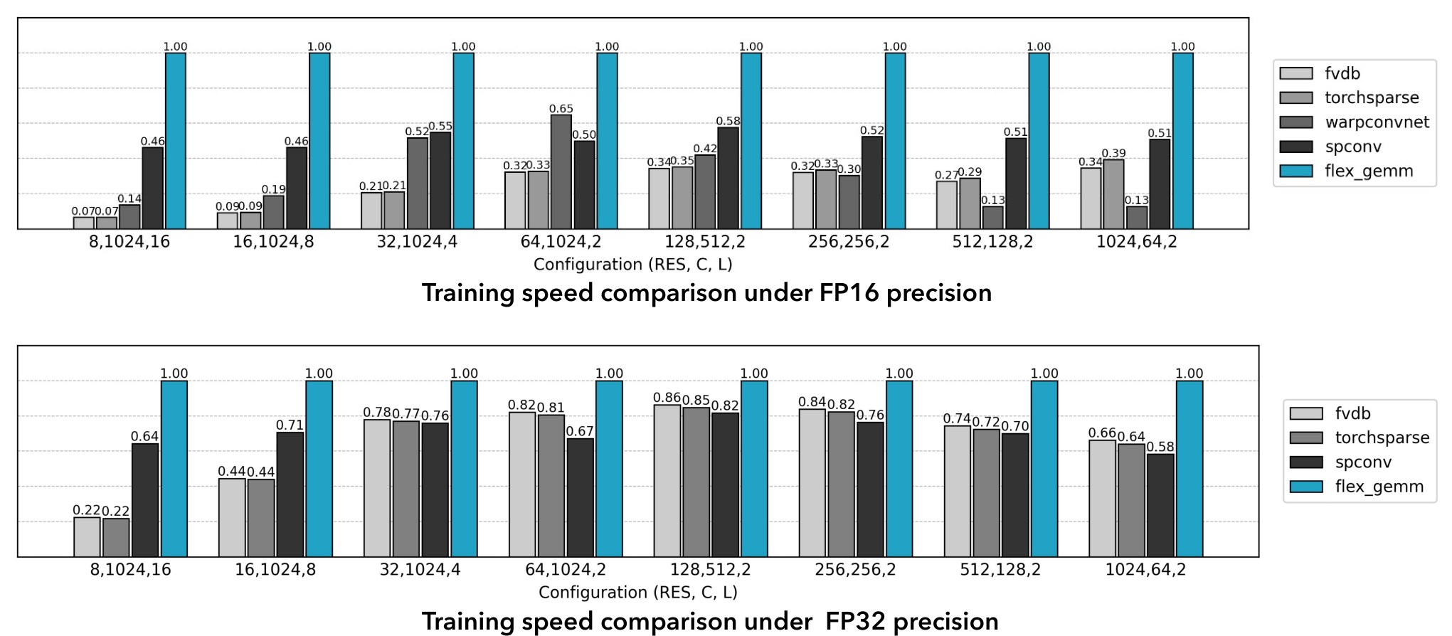
Figure 9: Speed test for FlexGEMM backend and baselines including Spconv [11], Torchsparse [58], fvdb [62], and WarpConvNet [8]
图 9:FlexGEMM 后端与基线的速度测试,基线包括 Spconv [11]、Torchsparse [58]、fvdb [62] 和 WarpConvNet [8]。
The sparse convolutional networks in our model are accelerated by a custom high-performance backend developed for this work. This backend was engineered to address the performance and platform-dependency limitations of existing libraries, which are often tightly coupled to the NVIDIA CUDA ecosystem. By implementing our kernels in Triton [60], a high-level GPU programming language, we created a single, cross-platform codebase that delivers near-optimal performance on both NVIDIA and AMD hardware.
模型中的稀疏卷积网络由本工作开发的定制高性能后端加速。设计这一后端,是为了应对现有库在性能和平台依赖上的局限——这些库往往与 NVIDIA CUDA 生态紧密绑定。我们用高层 GPU 编程语言 Triton [60] 实现卷积核,从而得到一套跨平台代码,在 NVIDIA 和 AMD 硬件上都能接近最优性能。
Our final, optimized implementation employs a Masked Implicit GEMM strategy [11]. This approach moves beyond naive explicit matrix multiplication by fusing the feature gathering (im2col) and the matrix multiplication (GEMM) steps into a single, highly-optimized kernel. This fusion minimizes global memory I/O by keeping intermediate data in fast on-chip memory. To further enhance performance in sparse contexts, we introduce a masking mechanism that intelligently skips computation on empty neighbor slots. This is achieved by first reordering active voxels using Gray code ordering, a technique that groups voxels with similar neighborhood patterns together. This grouping significantly improves the SIMD efficiency of the GPU, reducing warp divergence and wasted computation. Finally, we incorporate a Split-K technique, which increases parallelism by dividing the accumulation dimension of the matrix multiplication into independent parallel tasks. This is particularly effective in common scenarios, such as those with a large number of channels or a small number of active voxels. The combination of these techniques results in a highly efficient backend, yielding up to a 2 speedup over widely-used sparse convolution libraries in our benchmarking (see Fig. 9).
最终优化后的实现采用掩码隐式 GEMM策略 [11]。该方法不再做朴素的显式矩阵乘法,而是把特征汇集(im2col)与矩阵乘法(GEMM)融合进同一个高度优化的核函数。这种融合把中间数据留在快速的片上内存中,从而减少全局内存读写。为在稀疏场景下进一步提高性能,我们引入掩码机制,智能跳过空邻域槽位上的计算。具体做法是先用格雷码排序重排活跃体素,把邻域模式相近的体素分到一起。这种分组显著提高 GPU 的 SIMD 效率,减少线程束分化和无效计算。最后,我们加入 Split-K 技术,把矩阵乘法的累加维拆成相互独立的并行任务,从而增加并行度。这在通道数较多或活跃体素较少等常见情形下尤其有效。这些技术合在一起,构成高效的后端。在我们的基准测试中,相比广泛使用的稀疏卷积库,最高可达到 加速(见图 9)。
Appendix C Data Preparation Details
附录 C 数据准备细节
| Source | Shape Availible | Material Availible |
|---|---|---|
| TexVerse [77] | 503387 | 382996 |
| ObjaverseXL (sketchfab) [12] | 168307 | 141623 |
| ObjaverseXL (github) [12] | 293887 | 202188 |
| ABO [9] | 4485 | 4485 |
| HSSD [28] | 6670 | 6670 |
| SC-VAE training set | 473349 | 354966 |
| All training set | 976736 | 737962 |
| Toys4k [56] (evaluation set) | 3229 | 2282 |
Table 6: Composition of the training set and evaluation set.
| 来源 | 可用形状 | 可用材质 |
|---|---|---|
| TexVerse [77] | 503387 | 382996 |
| ObjaverseXL (sketchfab) [12] | 168307 | 141623 |
| ObjaverseXL (github) [12] | 293887 | 202188 |
| ABO [9] | 4485 | 4485 |
| HSSD [28] | 6670 | 6670 |
| SC-VAE 训练集 | 473349 | 354966 |
| 全部训练集 | 976736 | 737962 |
| Toys4k [56](评测集) | 3229 | 2282 |
表 6:训练集与评测集的构成。
The data preparation pipeline is largely based on the setup proposed in Trellis [65]. We begin by curating a collection of 3D assets but exclude the 3D-FUTURE [17] dataset due to its lack of Physically-Based Rendering (PBR) materials. The remaining assets form the basis for training our SC-VAEs.
数据准备流程大体沿用 Trellis [65] 提出的设置。我们先整理一组三维资产,但因缺少物理渲染(PBR)材质而排除 3D-FUTURE [17] 数据集。其余资产构成训练 SC-VAE 的基础。
All assets in this curated collection are used to extract geometric data for training the shape SC-VAE. For the material SC-VAE, a more specific filtering process is required. We employ a custom Blender [10] script to parse materials from the raw assets and retain only those that utilize a standard metallic-roughness PBR workflow. This filtering process yields a subset of approximately 350,000 assets suitable for training the material VAE.
该精选集合中的全部资产都用于提取几何数据,以训练形状 SC-VAE。材质 SC-VAE 则需要更专门的过滤。我们用自定义的 Blender [10] 脚本解析原始资产中的材质,只保留采用标准金属度–粗糙度 PBR 工作流的资产。过滤后得到约 35 万张适合训练材质 VAE 的资产子集。
To train the generative models, we further augment the dataset with TexVerse [77] to increase the diversity of high-quality PBR materials. As a final quality control step, we filter the assets based on an aesthetic score. For simplicity, we leverage the thumbnail images provided on the Sketchfab [55] platform to estimate this score. Objects with an estimated aesthetic score below 4.5 are excluded from the training set. Detailed statistics of the final dataset are provided in Table 6.
为训练生成模型,我们进一步用 TexVerse [77] 扩充数据集,以增加高质量 PBR 材质的多样性。作为最后的质量控制步骤,我们按美学分数过滤资产。为简便起见,我们借助 Sketchfab [55] 平台提供的缩略图来估计该分数。估计美学分数低于 4.5 的物体被排除在训练集之外。最终数据集的详细统计见表 6。
To generate the image prompts required for training our image-conditioned model, we render a diverse set of views for each 3D asset using Blender. We apply a series of augmentations during this rendering process to ensure the model is robust against common ambiguities found in real-world inputs. Key augmentations include:
为给图像条件模型的训练生成图像提示,我们用 Blender 为每张三维资产渲染一组多样的视图。渲染过程中施加一系列增强,使模型对现实输入中常见的含混情况更稳健。主要增强包括:
- • Field of View (FoV): The camera’s Field of View (FoV) is randomly sampled between and . This augmentation is designed to make the model robust to variations in camera intrinsics, which are often unknown in practice.
- • 视场角(FoV): 相机视场角在 到 之间随机采样。这一增强旨在使模型对相机内参变化更稳健,而实践中内参往往未知。
- • Lighting Conditions: The lighting environment is randomized by ramdomly placing and adjusting the intensity of light sources. This improves the model’s ability to predict intrinsic PBR attributes accurately, disentangling them from environmental illumination.
- • 光照条件: 通过随机放置光源并调节其强度,对光照环境做随机化。这提高了模型准确预测固有 PBR 属性的能力,把它们与环境照明分离开来。
Appendix D More Experiment Details
附录 D 更多实验细节
D.1 Evaluation Protocol
D.1 评测协议
In the main paper, we present quantitative comparisons and ablation studies using a series of numerical metrics. We provide the detailed protocols for their calculation below.
正文中,我们用一系列数值指标给出定量比较和消融研究。下面提供这些指标的详细计算协议。
Test set.
To ensure a robust evaluation of reconstruction quality, we prepared two distinct test sets.
测试集。
为稳健评估重建质量,我们准备了两个不同的测试集。
- • Toys4k-PBR. Our first test set is derived from the Toys4k dataset. For a rigorous metric, we filtered the raw assets to include only those containing all three standard PBR maps (base color, metallic, and roughness). This process resulted in a refined test set of 473 instances.
- • Toys4k-PBR。 第一个测试集来自 Toys4k 数据集。为使指标更严格,我们过滤原始资产,只保留同时包含全部三种标准 PBR 贴图(基础色、金属度和粗糙度)的样本。过滤后得到包含 473 个实例的精炼测试集。
- • Sketchfab Featured. Recognizing that the assets in Toys4k are relatively simple, we curated a second, more challenging test set from high-quality, recent assets on Sketchfab. Specifically, we selected models from the “Staff Picks” category, which features professionally curated content. We then applied a filter to retain only assets that utilize the metallic-roughness PBR workflow and were uploaded within the last two years. This process yielded a high-quality test set comprising 90 instances, designed to evaluate performance on complex, professional-grade assets.
- • Sketchfab Featured。 鉴于 Toys4k 中的资产相对简单,我们从 Sketchfab 上近期的高质量资产中整理出第二个、更具挑战性的测试集。具体而言,我们从“Staff Picks”类别中选取模型,该类别展示经专业挑选的内容。随后再过滤,只保留采用金属度–粗糙度 PBR 工作流、且在近两年内上传的资产。最终得到包含 90 个实例的高质量测试集,用于评估方法在复杂、专业级资产上的表现。
Geometry Accuracy.
To assess the overall geometric fidelity, we use Mesh Distance and the corresponding F-score. Unlike Chamfer Distance, which is sensitive to point cloud density, Mesh Distance provides a more stable measure of the discrepancy between two triangle meshes. This makes it particularly suitable for evaluating reconstruction accuracy across all surfaces, including those that are fully enclosed. For this evaluation, we sample 1 million points from the surface of each mesh. For the F-score calculation, we use a distance threshold of .
几何精度。
为评估整体几何保真度,我们使用*网格距离(Mesh Distance)*及相应的 F 分数。与对点云密度敏感的 Chamfer 距离不同,网格距离对两张三角网格之间差异的度量更稳定。因此,它特别适合评估包括完全封闭表面在内的全部表面的重建精度。评测时,我们从每张网格的表面采样 100 万个点。计算 F 分数时,距离阈值为 。
For evaluating the accuracy of visible surfaces, we compute Chamfer Distance (CD) and the corresponding F-score. The evaluation is performed on point clouds generated by sampling the outer shell of the meshes. Specifically, we render depth maps for each mesh from 100 uniformly sampled camera views. These depth maps are then unprojected to create a dense 3D point cloud, from which we randomly sample 1 million points. For the F-score calculation, we use a distance threshold of .
为评估可见表面的精度,我们计算 Chamfer 距离(CD) 及相应的 F 分数。评测在从网格外壳采样得到的点云上进行。具体而言,我们从 100 个均匀采样的相机视角为每张网格渲染深度图。再把这些深度图反投影,形成稠密三维点云,并从中随机采样 100 万个点。计算 F 分数时,距离阈值为 。
To evaluate the quality of fine surface details, we compute PSNR and LPIPS on rendered normal maps. For this, we render images from four fixed camera positions for all assets. The camera is placed on a sphere of radius 10 with a fixed pitch angle of and a narrow Field of View (FoV) of . The four views correspond to yaw angles of and .
为评估细表面细节的质量,我们在渲染的法向图上计算 PSNR 和 LPIPS。为此,我们对所有资产从四个固定相机位置渲染图像。相机放在半径为 10 的球面上,俯仰角固定为 ,视场角较窄,为 。四个视图对应的偏航角分别为 、、 和 。
Prior to any metric calculation, all ground-truth and predicted meshes are normalized to fit within a unit cube. The definitions for the geometric metrics are as follows:
在计算任何指标之前,所有真值网格和预测网格都被归一化到单位立方体内。几何指标的定义如下:
- • Mesh Distance (MD). MD is calculated as the bidirectional point-to-mesh surface distance, averaged over a dense sampling of points from both meshes. Given two meshes and , with sampled points and , MD is defined as: (10)
- • 网格距离(MD)。 MD 按双向点到网格表面距离计算,并在从两张网格稠密采样的点上取平均。给定两张网格 和 ,以及采样点 和 ,MD 定义为: (10)
- • Chamfer Distance (CD). Given two point clouds, and , the Chamfer Distance is defined as: (11)
- • Chamfer 距离(CD)。 给定两个点云 和 ,Chamfer 距离定义为: (11)
- • F-score. The F-score evaluates shape correspondence by combining precision and recall, calculated based on a distance threshold . Given a ground-truth shape and a predicted shape , we sample point sets from and from . Precision and Recall are then defined as: (12) where is the indicator function and is the minimum Euclidean distance from a point to the shape . The F-score is the harmonic mean of these values: (13) The distance function is defined differently depending on the context, described below. – For CD F-score: The shapes and are treated as discrete point clouds. The distance is the Euclidean distance from point to the nearest point within the point cloud . – For MD F-score: The shapes and are treated as continuous triangle meshes. The distance is the Euclidean distance from point to the closest point on the surface of the mesh .
- • F 分数。 F 分数通过结合精确率和召回率来评估形状对应关系,二者均基于距离阈值 计算。给定真值形状 和预测形状 ,我们分别从 和 采样点集 和 。精确率和召回率定义为: (12)其中 是指示函数, 是点 到形状 的最小欧氏距离。F 分数是二者的调和平均: (13)距离函数 随具体情形而定义,说明如下。– 对 CD 的 F 分数:形状 和 被看作离散点云。距离 是点 到点云 中最近点的欧氏距离。– 对 MD 的 F 分数:形状 和 被看作连续三角网格。距离 是点 到网格 表面上最近点的欧氏距离。
Appearance Fidelity.
To assess the quality of the reconstructed materials, we evaluate both the raw PBR attribute maps and the final shaded images. For both the ground-truth and the reconstructed 3D assets, we render two sets of images using the nvdiffrec renderer [44]. This rendering is performed using the same fixed-camera setup as the normal map evaluation, capturing four distinct views. The PSNR and LPIPS metrics are then calculated by comparing the rendered outputs from the reconstructed asset against those from the ground truth. The final reported scores are the average values across these four views.
外观保真度。
为评估重建材质的质量,我们同时评测原始 PBR 属性图和最终着色图像。对真值和重建的三维资产,我们都用 nvdiffrec 渲染器 [44] 渲染两组图像。渲染采用与法向图评测相同的固定相机设置,拍摄四个不同视图。随后通过比较重建资产与真值的渲染输出,计算 PSNR 和 LPIPS。最终报告的分数是这四个视图上的平均值。
Test Set.
For quantitative evaluation of our image-to-3D generation capabilities, we conduct experiments on a challenging test set of 100 image prompts generated by the NanoBanana text-to-image model [16]. This dataset was specifically chosen for its diversity and complexity. It features prompts that describe objects with intricate geometries, varied and dramatic lighting conditions, and a wide range of realistic materials, including metal, leather, rust, and translucent substances such as glass.
测试集。
为定量评估图像到三维生成能力,我们在一组具有挑战性的测试集上做实验,其中包含 100 张由 NanoBanana 文生图模型 [16] 生成的图像提示。选择该数据集,是因为它多样且复杂。其中的提示描述了具有精细几何、多变而强烈的光照,以及金属、皮革、锈蚀和玻璃等半透明物质在内的多种真实材质的物体。
Evaluation Metrics.
We employ a suite of metrics targeting different aspects of the output. The visual and semantic alignment between the input image prompt and rendered images of the asset is measured using the CLIP score [50]. To evaluate how well the 3D geometry and appearance properties match the image prompt, we use the multimodal foundation models ULIP-2 [67] and Uni3D [80]. Details of the metrics are listed below:
评测指标。
我们采用一组面向输出不同方面的指标。输入图像提示与资产渲染图像之间的视觉和语义对齐,用 CLIP 分数 [50] 衡量。为评估三维几何和外观属性与图像提示的匹配程度,我们使用多模态基础模型 ULIP-2 [67] 和 Uni3D [80]。各指标细节如下:
- • CLIP Score. The CLIP score measures the semantic similarity between two images. In our evaluation, we render the generated 3D asset from 4 predefined viewpoints (same yaw, pitch setup as previous metrics). We then compute the average cosine similarity between the CLIP embedding of the input image prompt and the rendered images (or normal map). A higher CLIP score indicates a better semantic alignment between the conditional input and the appearance (or geometry) of the generated asset.
- • CLIP 分数。 CLIP 分数衡量两张图像之间的语义相似度。评测中,我们从 4 个预定义视角渲染生成的三维资产(偏航角、俯仰角设置与前述指标相同)。随后计算输入图像提示的 CLIP 嵌入与渲染图像(或法向图)之间的平均余弦相似度。CLIP 分数越高,说明条件输入与生成资产的外观(或几何)在语义上对齐得越好。
- • ULIP-2 and Uni3D Scores. ULIP-2 and Uni3D are models designed to understand and align 3D content with text/image . To prepare the input for these models, we first convert our generated mesh into a colored point cloud. Specifically, we uniformly sample 10,000 points from the surface of the mesh with Farthest Point Sampling. The color for each point is determined by querying its corresponding RGB value from the asset’s base color map. This colored point cloud is then fed into the ULIP-2 and Uni3D models to compute a similarity score against the image prompt. These scores provide a quantitative measure of how well the generated asset align with the condition from a native 3D perspective.
- • ULIP-2 与 Uni3D 分数。 ULIP-2 和 Uni3D 是用于理解三维内容并使其与文本/图像对齐的模型。为准备这些模型的输入,我们先把生成的网格转换成带颜色的点云。具体而言,我们用最远点采样从网格表面均匀采样 10,000 个点。每个点的颜色通过查询资产基础色图中对应的 RGB 值确定。随后把该带色点云输入 ULIP-2 和 Uni3D,计算其与图像提示的相似度分数。这些分数从原生三维的角度,定量衡量生成资产与条件的对齐程度。
D.2 User Study
D.2 用户研究
While quantitative metrics provide objective measurements of fidelity, they often fail to capture the nuanced perceptual qualities that define a high-quality 3D asset, such as aesthetic appeal and fine-detail plausibility. To provide a comprehensive evaluation that aligns with human perception, we conducted a rigorous user study to compare our method against others.
定量指标能给出保真度的客观度量,但往往难以抓住定义高质量三维资产的细微感知性质,例如审美感受和细节点是否合理。为提供与人的感知相一致的综合评价,我们做了严格的用户研究,将本方法与其他方法比较。
Figure 10: The interface for our user study. Participants were presented with two types of questions: one for evaluating the overall quality of fully rendered assets (top) and another for assessing the shape quality using normal map visualizations (bottom). The interface provided interactive controls for a thorough inspection.
图 10:用户研究界面。参与者会看到两类问题:一类评估完整渲染资产的总体质量(上),另一类借助法向图可视化评估形状质量(下)。界面提供交互控件,便于仔细检查。
Study Design and Interface.
Our study was designed to assess two critical aspects of 3D asset quality: overall quality (combining geometry and appearance) and shape quality (isolating geometric fidelity). Participants were presented with a series of choice questions through a custom web interface, as shown in Figure 10.
研究设计与界面。
本研究旨在评估三维资产质量的两个关键方面:总体质量(综合几何与外观)和形状质量(单独考察几何保真度)。参与者通过自定义网页界面回答一系列选择题,如图 10 所示。
For each question, participants were shown a reference image and a set of turntable video renderings of the 3D models generated by different methods. The interface provided interactive controls, allowing users to play, pause, scrub through the animation timeline, and zoom in to inspect details closely. This ensured that participants could perform a thorough comparison. The positions of the generated models were randomized for each question to prevent positional bias.
对每个问题,参与者会看到一张参考图像,以及由不同方法生成的三维模型的转盘视频渲染。界面提供交互控件,允许用户播放、暂停、在动画时间轴上拖动,以及放大以仔细检查细节。这保证参与者能够做充分比较。每个问题中,生成模型的位置都是随机的,以避免位置偏差。
The study consisted of two distinct types of questions:
研究包含两类不同的问题:
- • Overall Quality Evaluation: In this task, participants were shown fully textured and rendered 3D models. They were instructed to select the model with the “highest overall quality that best matches the object in the input image.” The evaluation criteria emphasized a holistic assessment, including accurate shape, high-definition textures, realistic material properties (reflection and transmission), and consistent appearance with the reference.
- • 总体质量评估: 在这一任务中,参与者看到完整带纹理并完成渲染的三维模型。他们被要求选出“总体质量最高、且与输入图像中物体最匹配”的模型。评测标准强调整体判断,包括形状准确、纹理清晰、材质属性真实(反射与透射),以及与参考图外观一致。
- • Shape Quality Evaluation: To specifically evaluate geometric accuracy without the confounding influence of materials, this task presented the models rendered with only a normal map. Participants were asked to select the model with the best shape, focusing on criteria such as “a well-defined shape, high-definition detail, sharp edges, and clear boundaries.”
- • 形状质量评估: 为在不受材质干扰的情况下专门评估几何精度,这一任务只用法向图渲染模型。参与者被要求选出形状最好的模型,关注“形状明确、细节清晰、边缘锐利、边界清楚”等标准。
| Method | Overall | Shape | ||
|---|---|---|---|---|
| Not Sure | 4 | 2.0% | 3 | 1.4% |
| Trellis | 13 | 6.4% | 6 | 2.8% |
| Hi3DGen | – | – | 14 | 6.6% |
| Direct3D-S2 | – | – | 26 | 12.2% |
| Step1X-3D | 24 | 11.8% | 1 | 0.5% |
| Hunyuan3D 2.1 | 27 | 13.3% | 16 | 7.5% |
| Ours | 135 | 66.5% | 147 | 69.0% |
| Total | 202 | 100% | 213 | 100% |
Table 7: Detailed statistics of the user study.
| 方法 | 总体 | 形状 | ||
|---|---|---|---|---|
| 不确定 | 4 | 2.0% | 3 | 1.4% |
| Trellis | 13 | 6.4% | 6 | 2.8% |
| Hi3DGen | – | – | 14 | 6.6% |
| Direct3D-S2 | – | – | 26 | 12.2% |
| Step1X-3D | 24 | 11.8% | 1 | 0.5% |
| Hunyuan3D 2.1 | 27 | 13.3% | 16 | 7.5% |
| 本文 | 135 | 66.5% | 147 | 69.0% |
| 合计 | 202 | 100% | 213 | 100% |
表 7:用户研究的详细统计。
Detailed Analysis.
We recruited about 40 participants in the evaluation. For each question, the model selected by a participant was recorded as a “win” over the other options presented. We aggregated these results from all participants and computed a global preference rate for each method. This percentage provides a clear ranking of perceptual quality. Detailed statistics of the user study are shown in Table 7.
详细分析。
我们招募了约 40 名参与者参加评测。对每个问题,参与者选出的模型被记为相对其他选项的一次“胜出”。我们汇总全部参与者的结果,并计算每种方法的全局偏好率。该百分比给出感知质量的清晰排序。用户研究的详细统计见表 7。
Appendix E More Results
附录 E 更多结果
E.1 3D Asset Reconstruction
E.1 三维资产重建
Additional Reconstruction Results.
We present additional reconstruction results of our SC-VAE in Figure 11. The figure showcases the model’s ability to achieve high-fidelity reconstruction across a diverse range of 3D assets. Our method successfully captures hard-surface mechanical objects (a combat mech), intricate thin structures (a shopping cart, a ferris wheel), open surfaces (a plant), words (a fridge), and complex material properties (a crystal). Despite the highly compact nature of the learned latent space, the model faithfully recovers both complex geometries, visualized via normal maps, and detailed PBR materials, shown in the final renders.
更多重建结果。
图 11 给出 SC-VAE 的更多重建结果。该图展示了模型在多样三维资产上实现高保真重建的能力。本方法成功捕获硬表面机械物体(一台作战机甲)、精细薄结构(一辆购物车、一座摩天轮)、开放面(一株植物)、文字(一台冰箱),以及复杂材质属性(一块晶体)。尽管学到的潜在空间高度紧凑,模型仍能忠实恢复复杂几何(用法向图可视化)和细致的 PBR 材质(见最终渲染)。
Additional Qualitative Comparisons.
Figure 12 provides an extended qualitative comparison of shape reconstruction fidelity against several state-of-the-art methods. The comparison includes normal map renderings, magnified insets to highlight fine details, and corresponding error maps that visualize the deviation from the ground truth. Across all examples, our method consistently demonstrates a superior ability to preserve high-frequency geometric details. For instance, our model more accurately reconstructs the intricate chainmail links of the helmet and the sharp ornamental patterns on the decorative vessel, where other methods often produce overly smooth or blurry surfaces. Notably, as demonstrated in the final column, our method also excels at recovering enclosed internal structures, which pose a significant challenge for many surface reconstruction techniques. This high fidelity is further corroborated by the error maps, which show visibly lower reconstruction errors for our method across all examples when compared to the baselines.
更多定性比较。
图 12 给出与若干先进方法在形状重建保真度上的扩展定性比较。比较包括法向图渲染、用于突出细部的放大插图,以及可视化相对真值偏差的误差图。在全部示例中,本方法在保留高频几何细节上始终表现更好。例如,我们的模型更准确地重建了头盔上精细的锁子甲链环,以及装饰器皿上锐利的纹样;其他方法则常常得到过于平滑或模糊的表面。值得注意的是,如最后一列所示,本方法也善于恢复封闭的内部结构,这对许多表面重建技术都是显著挑战。误差图进一步印证了这一高保真度:与各基线相比,本方法在全部示例上的重建误差都明显更低。
E.2 Image to 3D Asset Generation
E.2 图像到三维资产生成
Additional Generation Results.
We present additional qualitative results from our image-to-3D generation method in Figure 13. The figure demonstrates the model’s versatility and robustness across a wide range of categories, including organic structures (a garden trellis with ivy), complex hard-surface machinery (a sci-fi pod, a bulldozer), and detailed characters (a dwarf blacksmith, a soldier). For each generated asset, we display the final physically-based render, the corresponding normal map to illustrate geometric detail, and a breakdown of the constituent PBR attribute maps along with relighting results. This comprehensive visualization highlights our method’s ability to jointly generate not only high-fidelity geometry but also plausible PBR materials that respond correctly to novel lighting conditions.
更多生成结果。
图 13 给出本方法图像到三维生成的更多定性结果。该图展示了模型在广泛类别上的适应力和稳健性,包括有机结构(带常春藤的园艺棚架)、复杂的硬表面机械(一艘科幻舱体、一台推土机),以及细致的角色(一名矮人铁匠、一名士兵)。对每张生成资产,我们展示最终的物理渲染、用于说明几何细节的对应法向图,以及组成性 PBR 属性图的分解和重新打光结果。这一全面可视化突出表明,本方法不仅能联合生成高保真几何,也能生成在新光照条件下响应正确的合理 PBR 材质。
Additional Qualitative Comparisons.
In Figure 14, we provide further qualitative comparisons for the image-to-3D generation task against several recent state-of-the-art methods. A primary advantage of our method is its ability to generate high-quality PBR materials, a capability not present in several baselines such as Step1X-3D, TRELLIS, Direct3D-S2, and Hi3DGen. When comparing geometric fidelity via the normal maps, our results consistently exhibit sharper and more coherent details. For example, our method more accurately captures the fine mechanical joints of the crab and the face of the character, whereas competing methods often produce results that are overly smoothed or contain noticeable artifacts. Furthermore, for methods that do produce PBR materials (Hunyuan3D 2.1), our approach generates textures that are visually more plausible and better aligned with the input prompts.
更多定性比较。
在图 14 中,我们给出图像到三维生成任务上与若干近期先进方法的进一步定性比较。本方法的一项主要优势,是能够生成高质量 PBR 材质;Step1X-3D、TRELLIS、Direct3D-S2 和 Hi3DGen 等若干基线并不具备这一能力。在通过法向图比较几何保真度时,我们的结果始终展现出更锐利、更连贯的细节。例如,本方法更准确地捕获了螃蟹精细的机械关节和角色的面部,而对照方法往往过于平滑,或带有明显伪影。此外,对于同样生成 PBR 材质的方法(Hunyuan3D 2.1),本方法给出的纹理在视觉上更合理,也与输入提示对齐得更好。
Appendix F Limitation Discussion and Future Work
附录 F 局限讨论与未来工作
Despite the promising results, our method has several limitations that open avenues for future research.
尽管结果令人鼓舞,本方法仍有若干局限,也为后续研究留下空间。
First, similar to other voxel-based methods, O-Voxel’s representation power is bounded by its spatial resolution. For detailed geometric features smaller than the voxel size, the Flexible Dual Grid formulation could produce aliasing artifacts. For example, when two parallel surfaces that are very close to each other intersect the same voxel, the QEF solver, by design, will place the dual vertex at a position that minimizes the error to both surfaces, often resulting in a vertex located between them rather than accurately on one. Similarly, the volumetric material attributes in such a voxel will be an average of the properties of both surfaces, leading to blurred appearance.
首先,与其他基于体素的方法类似,O-Voxel 的表示能力受其空间分辨率限制。对于小于体素尺寸的细致几何特征,灵活对偶网格表述可能产生走样伪影。例如,当两张非常靠近的平行表面穿过同一个体素时,QEF 求解器按设计会把对偶顶点放在使到两张表面的误差都尽量小的位置,结果往往是顶点落在二者之间,而不是准确地落在其中一张上。同样,该体素中的体材质属性会是两张表面属性的平均,从而导致外观模糊。
Second, we observe that the reconstructed and generated results sometimes contain small holes, though they can mostly be rectified with standard mesh post-processing techniques (e.g., hole filling). We attribute this issue to challenges in the sparse nature of our decoder, where ensuring a perfectly closed, manifold surface from the high-resolution sparse structure predicted by our decoder can be difficult. Improving the inherent stability of decoding process is an important area for improvement.
其次,我们观察到重建和生成结果有时会出现小孔,不过大多可用标准的网格后处理技术加以修正(例如补洞)。我们将这一问题归因于解码器稀疏性质带来的挑战:要从解码器预测的高分辨率稀疏结构中,确保得到完全封闭、流形的表面,并不容易。提高解码过程固有的稳定性,是一项重要的改进方向。
Finally, our O-Voxel is currently focused on geometry and material and it does not explicitly encode higher-level structural or semantic information. A significant direction for future research is to extend our representation to incorporate part-level segmentation and a graph-based topological structure. Such a structured representation would unlock an even wider range of downstream applications.
最后,当前的 O-Voxel 主要关注几何和材质,并不显式编码更高层的结构或语义信息。一个重要的未来研究方向,是扩展该表示,纳入部件级分割和基于图的拓扑结构。这样的结构化表示将为更广泛的下游应用打开空间。
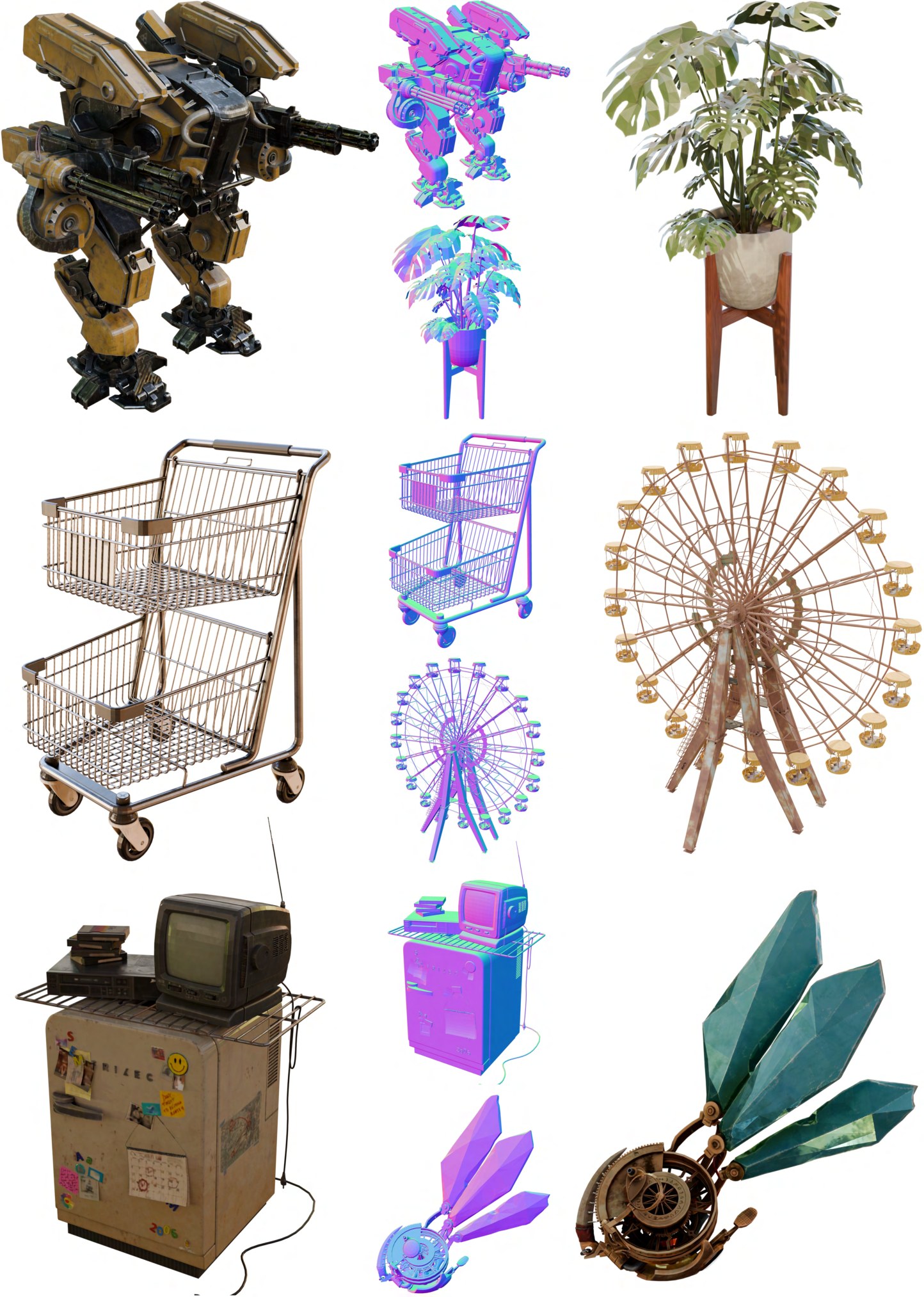
Figure 11: Reconstruction results of our method. Despite highly compact, it achieves high-fidelity recovery of complex shapes and materials.
图 11:本方法的重建结果。尽管表示高度紧凑,仍能高保真地恢复复杂形状与材质。
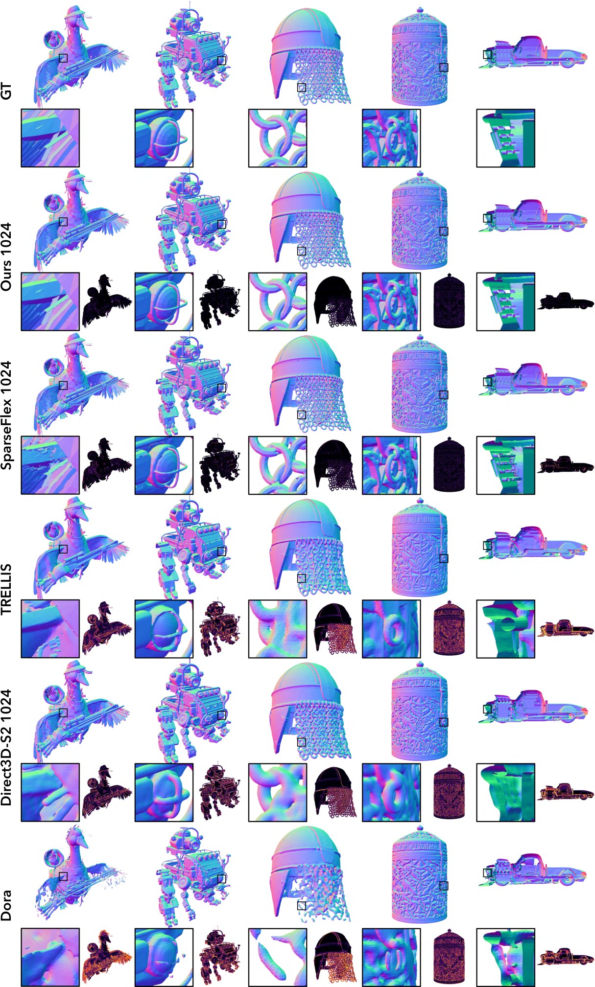
Figure 12: Qualitative comparison of shape reconstruction fidelity. Error maps are shown on the bottom right.
图 12:形状重建保真度的定性比较。误差图见右下。
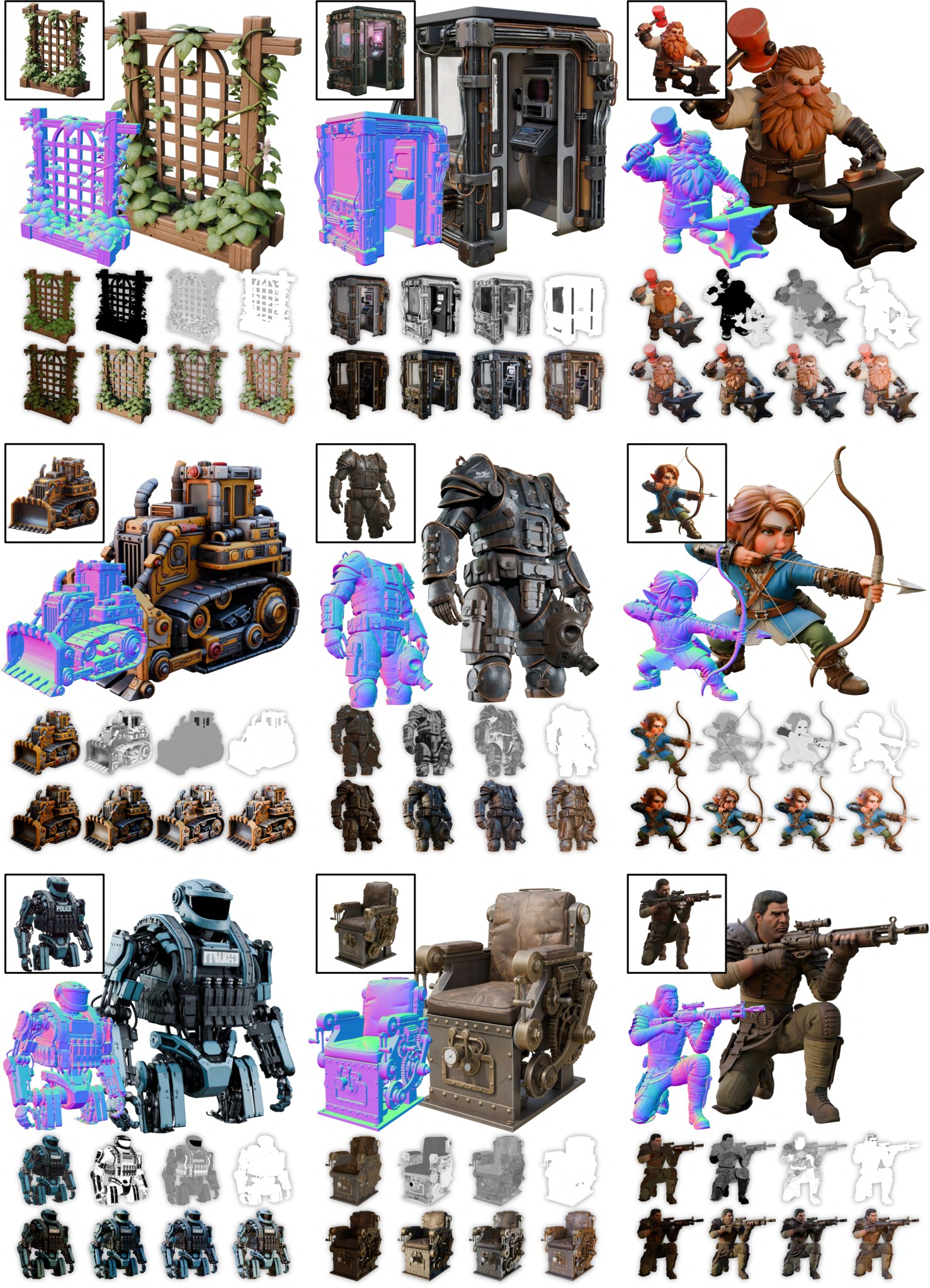
Figure 13: More image-to-3D generation results of our method. PBR attrbutes and relightings are shown below. (Best viewed with zoom)
图 13:本方法更多图像到三维生成结果。下方展示 PBR 属性和重新打光。(建议放大查看)
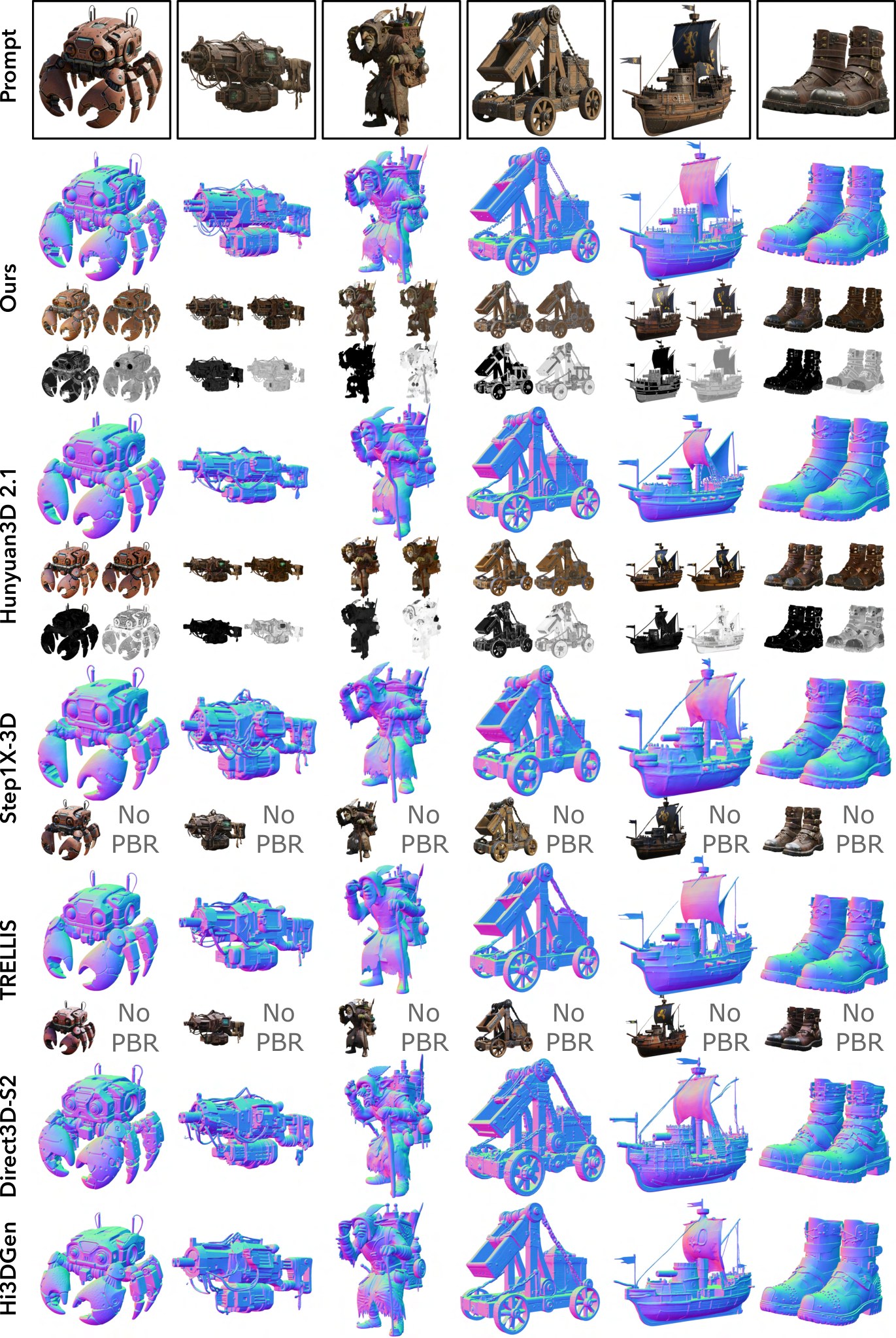
Figure 14: More comparisons of image-to-3D generation results. Rendering results and PBR attrbutes (if applicable) are shown below. (Best viewed with zoom)
图 14:更多图像到三维生成结果的比较。下方展示渲染结果以及 PBR 属性(如适用)。(建议放大查看)