Non-local Neural Networks

Xiaolong Wang 1 1 footnotemark: 1 Affiliation: Carnegie Mellon University Affiliation: Facebook AI Research    Ross Girshick Affiliation: Facebook AI Research    Abhinav Gupta Affiliation: Carnegie Mellon University    Kaiming He Affiliation: Facebook AI Research

Abstract

摘要

Both convolutional and recurrent operations are building blocks that process one local neighborhood at a time. In this paper, we present non-local operations as a generic family of building blocks for capturing long-range dependencies. Inspired by the classical non-local means method Buades2005 in computer vision, our non-local operation computes the response at a position as a weighted sum of the features at all positions. This building block can be plugged into many computer vision architectures. On the task of video classification, even without any bells and whistles, our non-local models can compete or outperform current competition winners on both Kinetics and Charades datasets. In static image recognition, our non-local models improve object detection/segmentation and pose estimation on the COCO suite of tasks. Code is available at https://github.com/facebookresearch/video-nonlocal-net.

卷积与循环运算都是一次只处理局部邻域的积木。本文提出非局部运算，作为一类通用积木，用来捕获长程依赖。受计算机视觉经典非局部均值方法（Buades2005）启发，非局部运算把某一位置的响应算成所有位置特征的加权和。该积木可插入多种视觉结构。在视频分类上，即便不加花哨技巧，非局部模型在 Kinetics 与 Charades 上也能比肩或超过当时竞赛优胜者。在静态图像识别中，非局部模型还提升了 COCO 上的目标检测/分割与姿态估计。代码见 https://github.com/facebookresearch/video-nonlocal-net。

1 Introduction

1 引言

Capturing long-range dependencies is of central importance in deep neural networks. For sequential data (e.g., in speech, language), recurrent operations Rumelhart1986; Hochreiter1997 are the dominant solution to long-range dependency modeling. For image data, long-distance dependencies are modeled by the large receptive fields formed by deep stacks of convolutional operations Fukushima1982; LeCun1989.

捕获长程依赖是深度网络的核心问题。对序列数据（如语音、语言），循环运算（Rumelhart1986；Hochreiter1997）是主流解法。对图像，长距离依赖则靠深层卷积堆叠形成的大感受野（Fukushima1982；LeCun1989）。

Convolutional and recurrent operations both process a local neighborhood, either in space or time; thus long-range dependencies can only be captured when these operations are applied repeatedly, propagating signals progressively through the data. Repeating local operations has several limitations. First, it is computationally inefficient. Second, it causes optimization difficulties that need to be carefully addressed Hochreiter1997; He2016. Finally, these challenges make multi-hop dependency modeling, e.g., when messages need to be delivered back and forth between distant positions, difficult.

卷积与循环都只处理局部邻域（空间或时间）；因此长程依赖只能靠反复施加这些运算、让信号在数据中逐步传递。重复局部运算有几处短板：一是计算不高效；二是会带来需仔细处理的优化困难（Hochreiter1997；He2016）；三是使多跳依赖建模变难——例如消息要在远距位置之间来回传递时。

In this paper, we present non-local operations as an efficient, simple, and generic component for capturing long-range dependencies with deep neural networks. Our proposed non-local operation is a generalization of the classical non-local mean operation Buades2005 in computer vision. Intuitively, a non-local operation computes the response at a position as a weighted sum of the features at all positions in the input feature maps (Figure 1). The set of positions can be in space, time, or spacetime, implying that our operations are applicable for image, sequence, and video problems.

本文提出非局部运算，作为捕获深度网络长程依赖的高效、简单且通用组件。它是视觉中经典非局部均值运算（Buades2005）的推广。直观上，某一位置的响应是输入特征图中所有位置特征的加权和（图 1）。位置集合可在空间、时间或时空上，因而适用于图像、序列与视频。

There are several advantages of using non-local operations: (a) In contrast to the progressive behavior of recurrent and convolutional operations, non-local operations capture long-range dependencies directly by computing interactions between any two positions, regardless of their positional distance; (b) As we show in experiments, non-local operations are efficient and achieve their best results even with only a few layers (e.g., 5); (c) Finally, our non-local operations maintain the variable input sizes and can be easily combined with other operations (e.g., convolutions as we will use).

非局部运算有几项优点：(a) 与循环、卷积的逐步传播不同，它直接计算任意两位置的交互，与距离无关；(b) 实验表明它高效，哪怕只有少数几层（如 5 层）也能达到最佳结果；(c) 保持可变输入尺寸，并易于与其他运算（如卷积）组合。

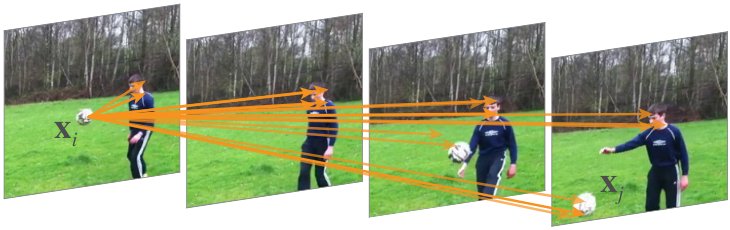
Figure 1: A spacetime non-local operation in our network trained for video classification in Kinetics. A position $\mathbf{x}_{i}$’s response is computed by the weighted average of the features of all positions $\mathbf{x}_{j}$ (only the highest weighted ones are shown here). In this example computed by our model, note how it relates the ball in the first frame to the ball in the last two frames. More examples are in Figure 3.

图 1：在 Kinetics 视频分类网络中的时空非局部运算。位置 $\mathbf{x}_{i}$ 的响应由所有位置 $\mathbf{x}_{j}$ 特征的加权平均得到（图中只画出权重最高的若干项）。本例中，模型把第一帧的球与最后两帧的球关联起来。更多例子见图 3。

We showcase the effectiveness of non-local operations in the application of video classification. In videos, long-range interactions occur between distant pixels in space as well as time. A single non-local block, which is our basic unit, can directly capture these spacetime dependencies in a feedforward fashion. With a few non-local blocks, our architecures called non-local neural networks are more accurate for video classification than 2D and 3D convolutional networks Tran2015 (including the inflated variant Carreira2017). In addition, non-local neural networks are more computationally economical than their 3D convolutional counterparts. Comprehensive ablation studies are presented on the Kinetics Kay2017 and Charades Sigurdsson2016 datasets. Using RGB only and without any bells and whistles (e.g., optical flow, multi-scale testing), our method achieves results on par with or better than the latest competitions winners on both datasets.

我们以视频分类展示非局部运算的效果。视频中，远距像素在空间与时间上都存在长程交互。单个非局部块（基本单元）即可前馈地直接捕获这些时空依赖。加入若干非局部块后，我们称为非局部神经网络的结构，在视频分类上比 2D 与 3D 卷积网络（Tran2015，含膨胀变体 Carreira2017）更准，也比 3D 卷积更省算力。我们在 Kinetics（Kay2017）与 Charades（Sigurdsson2016）上做了系统消融。只用 RGB、不加花哨技巧（如光流、多尺度测试），方法在两个数据集上都与最新竞赛优胜者持平或更好。

To demonstrate the generality of non-local operations, we further present object detection/segmentation and pose estimation experiments on the COCO dataset Lin2014. On top of the strong Mask R-CNN baseline He2017, our non-local blocks can increase accuracy on all three tasks at a small extra computational cost. Together with the evidence on videos, these image experiments show that non-local operations are generally useful and can become a basic building block in designing deep neural networks.

为说明通用性，我们还在 COCO（Lin2014）上做了目标检测/分割与姿态估计。在强 Mask R-CNN 基线（He2017）之上，非局部块以很小额外计算量提升三项任务精度。结合视频证据，这些图像实验表明非局部运算普遍有用，可成为深度网络设计的基本积木。

2 Related Work

2 相关工作

Non-local image processing.

Non-local means Buades2005 is a classical filtering algorithm that computes a weighted mean of all pixels in an image. It allows distant pixels to contribute to the filtered response at a location based on patch appearance similarity. This non-local filtering idea was later developed into BM3D (block-matching 3D) Dabov2007, which performs filtering on a group of similar, but non-local, patches. BM3D is a solid image denoising baseline even compared with deep neural networks Burger2012. Block matching was used with neural networks for image denoising Burger2012a; Lefkimmiatis2016. Non-local matching is also the essence of successful texture synthesis Efros1999, super-resolution Glasner2009, and inpainting Barnes2009 algorithms.

非局部图像处理。

非局部均值（Buades2005）是经典滤波：对图像中所有像素做加权平均，让远距像素按块外观相似度贡献到当前位置的滤波响应。该思想后来发展成 BM3D（Dabov2007），在一组相似但非局部的块上滤波；即便对比深度网络，BM3D 仍是扎实的去噪基线（Burger2012）。块匹配也曾与神经网络结合用于去噪（Burger2012a；Lefkimmiatis2016）。非局部匹配同样是纹理合成（Efros1999）、超分辨（Glasner2009）与修复（Barnes2009）等成功算法的核心。

Graphical models.

Long-range dependencies can be modeled by graphical models such as conditional random fields (CRF) Lafferty2001; Kraehenbuehl2011. In the context of deep neural networks, a CRF can be exploited to post-process semantic segmentation predictions of a network Chen2014. The iterative mean-field inference of CRF can be turned into a recurrent network and trained Zheng2015; Schwing2015; Chandra2017; Harley2017; Liu2017. In contrast, our method is a simpler feedforward block for computing non-local filtering. Unlike these methods that were developed for segmentation, our general-purpose component is applied for classification and detection. These methods and ours are also related to a more abstract model called graph neural networks Scarselli2009.

图模型。

长程依赖可用条件随机场（CRF）等图模型建模（Lafferty2001；Kraehenbuehl2011）。在深度网络语境下，CRF 可后处理语义分割预测（Chen2014）；CRF 的迭代均值场推断也可写成循环网络并端到端训练（Zheng2015；Schwing2015；Chandra2017；Harley2017；Liu2017）。相较之下，我们的方法是更简单的前馈块，做非局部滤波。这些方法多面向分割，而我们的通用组件用于分类与检测。它们与我们也都关联到更抽象的图神经网络（Scarselli2009）。

Feedforward modeling for sequences.

Recently there emerged a trend of using feedforward (i.e., non-recurrent) networks for modeling sequences in speech and language Oord2016; Xiong2016; Gehring2017. In these methods, long-term dependencies are captured by the large receptive fields contributed by very deep 1-D convolutions. These feedforward models are amenable to parallelized implementations and can be more efficient than widely used recurrent models.

序列的前馈建模。

近期语音与语言中出现用前馈（即非循环）网络建模序列的趋势（Oord2016；Xiong2016；Gehring2017）。这些方法靠极深一维卷积带来的大感受野捕获长期依赖，便于并行实现，往往比常用循环模型更高效。

Self-attention.

Our work is related to the recent self-attention Vaswani2017 method for machine translation. A self-attention module computes the response at a position in a sequence (e.g., a sentence) by attending to all positions and taking their weighted average in an embedding space. As we will discuss in the next, self-attention can be viewed as a form of the non-local mean Buades2005, and in this sense our work bridges self-attention for machine translation to the more general class of non-local filtering operations that are applicable to image and video problems in computer vision.

自注意力。

本工作与机器翻译中的自注意力（Vaswani2017）相关：序列中某一位置的响应通过对所有位置加权平均（在嵌入空间中）得到。下文会说明，自注意力可视为非局部均值（Buades2005）的一种形式；就此而言，我们把机器翻译里的自注意力桥接到更一般的非局部滤波，使其可用于视觉中的图像与视频问题。

Interaction networks.

Interaction Networks (IN) Battaglia2016; Watters2017 were proposed recently for modeling physical systems. They operate on graphs of objects involved in pairwise interactions. Hoshen Hoshen2017 presented the more efficient Vertex Attention IN (VAIN) in the context of multi-agent predictive modeling. Another variant, named Relation Networks Santoro2017, computes a function on the feature embeddings at all pairs of positions in its input. Our method also processes all pairs, as we will explain ($f(\mathbf{x}_{i},\mathbf{x}_{j})$ in Eq.(1)). While our non-local networks are connected to these approaches, our experiments indicate that the non-locality of the model, which is orthogonal to the ideas of attention/interaction/relation (e.g., a network can attend to a local region), is the key to their empirical success. Non-local modeling, a long-time crucial element of image processing (e.g., Efros1999; Buades2005), has been largely overlooked in recent neural networks for computer vision.

交互网络。

交互网络（IN，Battaglia2016；Watters2017）近来用于建模物理系统，在对象图上处理成对交互。Hoshen（Hoshen2017）在多智能体预测中提出更高效的顶点注意力 IN（VAIN）。另一变体关系网络（Santoro2017）对输入中所有位置对的特征嵌入计算函数。我们的方法也处理所有对，见式 (1) 中的 $f(\mathbf{x}_{i},\mathbf{x}_{j})$。虽与这些思路有联系，实验表明模型的非局部性——与注意力/交互/关系正交（例如网络也可以只关注局部区域）——才是经验成功的关键。非局部建模长期是图像处理的要素（如 Efros1999；Buades2005），却在近期视觉神经网络中被明显忽视。

Video classification architectures.

A natural solution to video classification is to combine the success of CNNs for images and RNNs for sequences Yue-HeiNg2015; Donahue2015. In contrast, feedforward models are achieved by 3D convolutions (C3D) Ji2010; Tran2015 in spacetime, and the 3D filters can be formed by “inflating” Feichtenhofer2016; Carreira2017 pre-trained 2D filters. In addition to end-to-end modeling on raw video inputs, it has been found that optical flow Simonyan2014 and trajectories Wang2013a; Wang2015 can be helpful. Both flow and trajectories are off-the-shelf modules that may find long-range, non-local dependency. A systematic comparison of video architectures can be found in Carreira2017.

视频分类结构。

自然做法是把图像 CNN 与序列 RNN 结合（Yue-HeiNg2015；Donahue2015）。前馈路线则用时空 3D 卷积（C3D，Ji2010；Tran2015），3D 滤波器可由预训练 2D 滤波器「膨胀」得到（Feichtenhofer2016；Carreira2017）。除在原始视频上端到端建模外，光流（Simonyan2014）与轨迹（Wang2013a；Wang2015）也被证明有帮助；二者都是可发现长程、非局部依赖的现成模块。系统比较见 Carreira2017。

3 Non-local Neural Networks

3 非局部神经网络

We first give a general definition of non-local operations and then we provide several specific instantiations of it.

我们先给出非局部运算的一般定义，再给出若干具体实例化。

3.1 Formulation

3.1 形式化

Following the non-local mean operation Buades2005, we define a generic non-local operation in deep neural networks as:

沿用非局部均值（Buades2005），我们在深度网络中定义通用非局部运算为：

$$\mathbf{y}_{i}=\frac{1}{\mathcal{C(\mathbf{x})}}\sum_{\forall j}f(\mathbf{x}_{i},\mathbf{x}_{j})g(\mathbf{x}_{j}). \tag{1}$$

Here $i$ is the index of an output position (in space, time, or spacetime) whose response is to be computed and $j$ is the index that enumerates all possible positions. $\mathbf{x}$ is the input signal (image, sequence, video; often their features) and $\mathbf{y}$ is the output signal of the same size as $\mathbf{x}$. A pairwise function $f$ computes a scalar (representing relationship such as affinity) between $i$ and all $j$. The unary function $g$ computes a representation of the input signal at the position $j$. The response is normalized by a factor $\mathcal{C}(\mathbf{x})$.

这里 $i$ 是待计算响应的输出位置索引（空间、时间或时空），$j$ 枚举所有可能位置。$\mathbf{x}$ 为输入信号（图像、序列、视频；往往是其特征），$\mathbf{y}$ 为与 $\mathbf{x}$ 同尺寸的输出。成对函数 $f$ 计算 $i$ 与各 $j$ 之间的标量（表示亲和等关系）；一元函数 $g$ 计算位置 $j$ 处的输入表示。响应用因子 $\mathcal{C}(\mathbf{x})$ 归一化。

The non-local behavior in Eq.(1) is due to the fact that all positions ($\forall j$) are considered in the operation. As a comparison, a convolutional operation sums up the weighted input in a local neighborhood (e.g., $i-1\leq j\leq i+1$ in a 1D case with kernel size 3), and a recurrent operation at time $i$ is often based only on the current and the latest time steps (e.g., $j=i$ or $i-1$).

式 (1) 的非局部性来自运算考虑了所有位置（$\forall j$）。对比之下，卷积只在局部邻域内对加权输入求和（如一维核大小 3 时 $i-1\leq j\leq i+1$）；时刻 $i$ 的循环运算往往只依赖当前与上一时刻（如 $j=i$ 或 $i-1$）。

The non-local operation is also different from a fully-connected (fc) layer. Eq.(1) computes responses based on relationships between different locations, whereas fc uses learned weights. In other words, the relationship between $\mathbf{x}_{j}$ and $\mathbf{x}_{i}$ is not a function of the input data in fc, unlike in non-local layers. Furthermore, our formulation in Eq.(1) supports inputs of variable sizes, and maintains the corresponding size in the output. On the contrary, an fc layer requires a fixed-size input/output and loses positional correspondence (e.g., that from $\mathbf{x}_{i}$ to $\mathbf{y}_{i}$ at the position $i$).

非局部运算也不同于全连接（fc）层。式 (1) 基于不同位置间的关系计算响应，而 fc 使用学到的权重。换言之，fc 中 $\mathbf{x}_{j}$ 与 $\mathbf{x}_{i}$ 的关系不是输入数据的函数，非局部层则是。此外，式 (1) 支持可变尺寸输入并在输出保持对应尺寸；fc 则要求固定尺寸，并丢失位置对应（如位置 $i$ 上从 $\mathbf{x}_{i}$ 到 $\mathbf{y}_{i}$）。

A non-local operation is a flexible building block and can be easily used together with convolutional/recurrent layers. It can be added into the earlier part of deep neural networks, unlike fc layers that are often used in the end. This allows us to build a richer hierarchy that combines both non-local and local information.

非局部运算是灵活积木，易于与卷积/循环层并用。它可加在深度网络靠前的部分，而不像常放在末端的 fc。这使得我们可以构建同时融合非局部与局部信息的更丰富层次。

3.2 Instantiations

3.2 实例化

Next we describe several versions of $f$ and $g$. Interestingly, we will show by experiments (Table 2a) that our non-local models are not sensitive to these choices, indicating that the generic non-local behavior is the main reason for the observed improvements.

接下来描述 $f$ 与 $g$ 的若干版本。有趣的是，实验（表 2a）表明非局部模型对这些选择并不敏感，说明观察到的提升主要来自通用的非局部行为。

For simplicity, we only consider $g$ in the form of a linear embedding: $g(\mathbf{x}_{j})=W_{g}\mathbf{x}_{j}$, where $W_{g}$ is a weight matrix to be learned. This is implemented as, e.g., 1$\times$1 convolution in space or 1$\times$1$\times$1 convolution in spacetime.

为简单起见，我们只考虑线性嵌入形式的 $g$：$g(\mathbf{x}_{j})=W_{g}\mathbf{x}_{j}$，其中 $W_{g}$ 为待学习权重矩阵。实现上例如空间上的 1$\times$1 卷积，或时空上的 1$\times$1$\times$1 卷积。

Next we discuss choices for the pairwise function $f$.

下面讨论成对函数 $f$ 的选择。

Gaussian.

Following the non-local mean Buades2005 and bilateral filters Tomasi1998, a natural choice of $f$ is the Gaussian function. In this paper we consider:

高斯。

沿用非局部均值（Buades2005）与双边滤波（Tomasi1998），$f$ 的自然选择是高斯函数。本文考虑：

$$f(\mathbf{x}_{i},\mathbf{x}_{j})=e^{\mathbf{x}_{i}^{T}\mathbf{x}_{j}}. \tag{2}$$

Here $\mathbf{x}_{i}^{T}\mathbf{x}_{j}$ is dot-product similarity. Euclidean distance as used in Buades2005; Tomasi1998 is also applicable, but dot product is more implementation-friendly in modern deep learning platforms. The normalization factor is set as $\mathcal{C}(\mathbf{x})=\sum_{\forall j}f(\mathbf{x}_{i},\mathbf{x}_{j})$.

这里 $\mathbf{x}_{i}^{T}\mathbf{x}_{j}$ 为点积相似度。Buades2005；Tomasi1998 中的欧氏距离也可用，但点积在现代深度学习平台上更易实现。归一化因子取 $\mathcal{C}(\mathbf{x})=\sum_{\forall j}f(\mathbf{x}_{i},\mathbf{x}_{j})$。

Embedded Gaussian.

A simple extension of the Gaussian function is to compute similarity in an embedding space. In this paper we consider:

嵌入高斯。

高斯的简单扩展是在嵌入空间中算相似度。本文考虑：

$$f(\mathbf{x}_{i},\mathbf{x}_{j})=e^{\theta(\mathbf{x}_{i})^{T}\phi(\mathbf{x}_{j})}. \tag{3}$$

Here $\theta(\mathbf{x}_{i})=W_{\theta}\mathbf{x}_{i}$ and $\phi(\mathbf{x}_{j})=W_{\phi}\mathbf{x}_{j}$ are two embeddings. As above, we set $\mathcal{C}(\mathbf{x})=\sum_{\forall j}f(\mathbf{x}_{i},\mathbf{x}_{j})$.

其中 $\theta(\mathbf{x}_{i})=W_{\theta}\mathbf{x}_{i}$，$\phi(\mathbf{x}_{j})=W_{\phi}\mathbf{x}_{j}$ 为两个嵌入。同上，$\mathcal{C}(\mathbf{x})=\sum_{\forall j}f(\mathbf{x}_{i},\mathbf{x}_{j})$。

We note that the self-attention module Vaswani2017 recently presented for machine translation is a special case of non-local operations in the embedded Gaussian version. This can be seen from the fact that for a given $i$, $\frac{1}{\mathcal{C}(\mathbf{x})}f(\mathbf{x}_{i},\mathbf{x}_{j})$ becomes the softmax computation along the dimension $j$. So we have $\mathbf{y}=\text{\emph{softmax}}(\mathbf{x}^{T}W^{T}_{\theta}W_{\phi}\mathbf{x})g(\mathbf{x})$, which is the self-attention form in Vaswani2017. As such, our work provides insight by relating this recent self-attention model to the classic computer vision method of non-local means Buades2005, and extends the sequential self-attention network in Vaswani2017 to a generic space/spacetime non-local network for image/video recognition in computer vision.

我们指出：*机器翻译中近期提出的自注意力模块（Vaswani2017）是嵌入高斯版非局部运算的特例。*对给定 $i$，$\frac{1}{\mathcal{C}(\mathbf{x})}f(\mathbf{x}_{i},\mathbf{x}_{j})$ 恰成为沿维 $j$ 的 softmax。于是 $\mathbf{y}=\text{\emph{softmax}}(\mathbf{x}^{T}W^{T}_{\theta}W_{\phi}\mathbf{x})g(\mathbf{x})$，即 Vaswani2017 中的自注意力形式。由此，本工作把近期自注意力模型与经典非局部均值（Buades2005）联系起来，并把 Vaswani2017 的序列自注意力网络推广为可用于图像/视频识别的通用空间/时空非局部网络。

Despite the relation to Vaswani2017, we show that the attentional behavior (due to softmax) is not essential in the applications we study. To show this, we describe two alternative versions of non-local operations next.

尽管与 Vaswani2017 有关，我们表明（由 softmax 带来的）注意力行为在所研究应用中并非本质。为此，下面再给出两种非局部运算的替代版本。

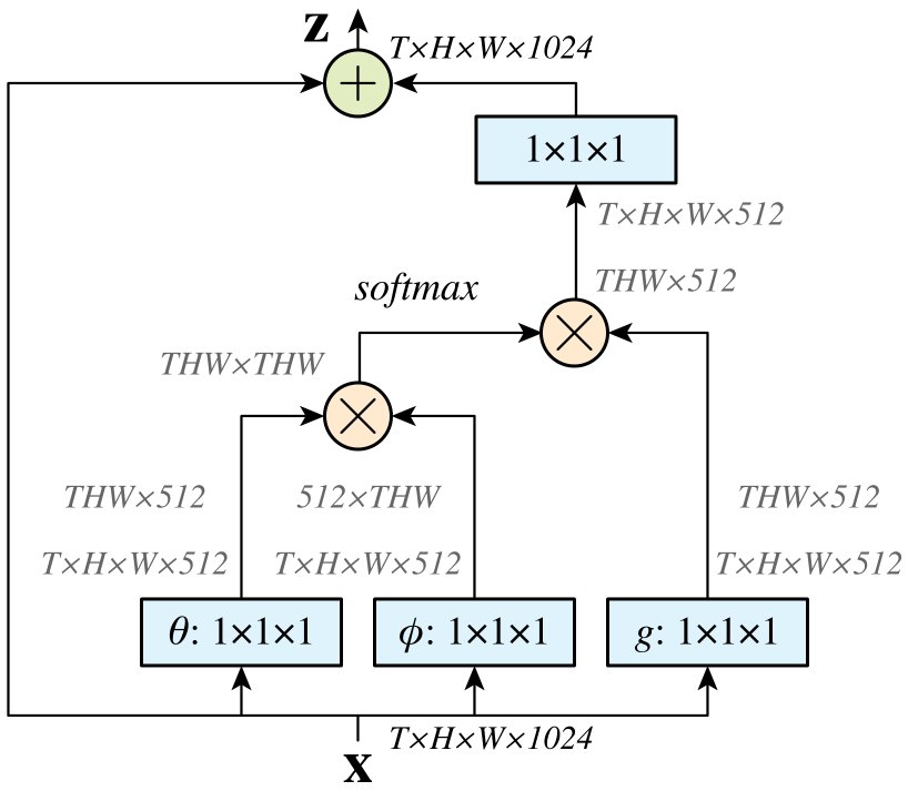
Figure 2: A spacetime non-local block. The feature maps are shown as the shape of their tensors, e.g., $T$$\times$$H$$\times$$W$$\times$$1024$ for 1024 channels (proper reshaping is performed when noted). “$\otimes$” denotes matrix multiplication, and “$\oplus$” denotes element-wise sum. The softmax operation is performed on each row. The blue boxes denote 1$\times$1$\times$1 convolutions. Here we show the embedded Gaussian version, with a bottleneck of 512 channels. The vanilla Gaussian version can be done by removing $\theta$ and $\phi$, and the dot-product version can be done by replacing softmax with scaling by $1/N$.

图 2：时空非局部块。特征图按其张量形状示意，如 1024 通道时为 $T$$\times$$H$$\times$$W$$\times$$1024$（必要时做适当重排）。「$\otimes$」表示矩阵乘，「$\oplus$」表示逐元素加。softmax 沿每一行执行。蓝色框为 1$\times$1$\times$1 卷积。图示为嵌入高斯版，瓶颈 512 通道。去掉 $\theta$ 与 $\phi$ 即得普通高斯版；把 softmax 换成按 $1/N$ 缩放即得点积版。

Dot product.

$f$ can be defined as a dot-product similarity:

点积。

$f$ 可定义为点积相似度：

$$f(\mathbf{x}_{i},\mathbf{x}_{j})=\theta(\mathbf{x}_{i})^{T}\phi(\mathbf{x}_{j}). \tag{4}$$

Here we adopt the embedded version. In this case, we set the normalization factor as $\mathcal{C}(\mathbf{x})=N$, where $N$ is the number of positions in $\mathbf{x}$, rather than the sum of $f$, because it simplifies gradient computation. A normalization like this is necessary because the input can have variable size.

这里采用嵌入版。归一化因子取 $\mathcal{C}(\mathbf{x})=N$，其中 $N$ 为 $\mathbf{x}$ 中的位置数，而非 $f$ 之和，以简化梯度计算。由于输入尺寸可变，这类归一化是必要的。

The main difference between the dot product and embedded Gaussian versions is the presence of softmax, which plays the role of an activation function.

点积版与嵌入高斯版的主要差别在于是否有 softmax；softmax 扮演激活函数的角色。

Concatenation.

Concatenation is used by the pairwise function in Relation Networks Santoro2017 for visual reasoning. We also evaluate a concatenation form of $f$:

拼接。

关系网络（Santoro2017）的成对函数使用拼接做视觉推理。我们也评估拼接形式的 $f$：

$$f(\mathbf{x}_{i},\mathbf{x}_{j})=\text{{ReLU}}(\mathbf{w}^{T}_{f}[\theta(\mathbf{x}_{i}),\penalty\ \phi(\mathbf{x}_{j})]). \tag{5}$$

Here $[\cdot,\cdot]$ denotes concatenation and $\mathbf{w}_{f}$ is a weight vector that projects the concatenated vector to a scalar. As above, we set $\mathcal{C}(\mathbf{x})=N$. In this case, we adopt ReLU Nair2010 in $f$.

其中 $[\cdot,\cdot]$ 表示拼接，$\mathbf{w}_{f}$ 为把拼接向量投影到标量的权重向量。同上，$\mathcal{C}(\mathbf{x})=N$。此时在 $f$ 中采用 ReLU（Nair2010）。

The above several variants demonstrate the flexibility of our generic non-local operation. We believe alternative versions are possible and may improve results.

以上若干变体展示了通用非局部运算的灵活性。我们相信还可有其他版本，并可能进一步提升结果。

3.3 Non-local Block

3.3 非局部块

We wrap the non-local operation in Eq.(1) into a non-local block that can be incorporated into many existing architectures. We define a non-local block as:

我们把式 (1) 的非局部运算包进可嵌入多种现有结构的非局部块，定义为：

$$\mathbf{z}_{i}=W_{z}\mathbf{y}_{i}+\mathbf{x}_{i}, \tag{6}$$

where $\mathbf{y}_{i}$ is given in Eq.(1) and “$+\mathbf{x}_{i}$” denotes a residual connection He2016. The residual connection allows us to insert a new non-local block into any pre-trained model, without breaking its initial behavior (e.g., if $W_{z}$ is initialized as zero). An example non-local block is illustrated in Figure 2. The pairwise computation in Eq.(2), (3), or (4) can be simply done by matrix multiplication as shown in Figure 2; the concatenation version in (5) is straightforward.

其中 $\mathbf{y}_{i}$ 由式 (1) 给出，「$+\mathbf{x}_{i}$」表示残差连接（He2016）。残差使我们可以把新非局部块插入任意预训练模型而不破坏初始行为（如若 $W_{z}$ 初始化为零）。图 2 给出示例非局部块。式 (2)(3)(4) 的成对计算可如图 2 用矩阵乘法完成；式 (5) 的拼接版也很直接。

The pairwise computation of a non-local block is lightweight when it is used in high-level, sub-sampled feature maps. For example, typical values in Figure 2 are $T=4$, $H=W=14$ or $7$. The pairwise computation as done by matrix multiplication is comparable to a typical convolutional layer in standard networks. We further adopt the following implementations that make it more efficient.

当非局部块用在高层、已下采样的特征图上时，成对计算很轻量。例如图 2 中典型取 $T=4$，$H=W=14$ 或 $7$。用矩阵乘法做的成对计算与标准网络中常见卷积层相当。我们还采用下列实现使其更高效。

Implementation of Non-local Blocks.

We set the number of channels represented by $W_{g}$, $W_{\theta}$, and $W_{\phi}$ to be half of the number of channels in $\mathbf{x}$. This follows the bottleneck design of He2016 and reduces the computation of a block by about a half. The weight matrix $W_{z}$ in Eq.(6) computes a position-wise embedding on $\mathbf{y}_{i}$, matching the number of channels to that of $\mathbf{x}$. See Figure 2.

非局部块的实现。

我们把 $W_{g}$、$W_{\theta}$、$W_{\phi}$ 表示的通道数设为 $\mathbf{x}$ 通道数的一半。这沿用 He2016 的瓶颈设计，约把一块的计算量减半。式 (6) 中的 $W_{z}$ 对 $\mathbf{y}_{i}$ 做逐位置嵌入，使通道数与 $\mathbf{x}$ 对齐。见图 2。

A subsampling trick can be used to further reduce computation. We modify Eq.(1) as: $\mathbf{y}_{i}=\frac{1}{\mathcal{C}(\mathbf{\hat{x}})}\sum_{\forall j}f(\mathbf{x}_{i},\mathbf{\hat{x}}_{j})g(\mathbf{\hat{x}}_{j})$, where $\mathbf{\hat{x}}$ is a subsampled version of $\mathbf{x}$ (e.g., by pooling). We perform this in the spatial domain, which can reduce the amount of pairwise computation by 1/4. This trick does not alter the non-local behavior, but only makes the computation sparser. This can be done by adding a max pooling layer after $\phi$ and $g$ in Figure 2.

还可用下采样技巧进一步降计算。把式 (1) 改为：$\mathbf{y}_{i}=\frac{1}{\mathcal{C}(\mathbf{\hat{x}})}\sum_{\forall j}f(\mathbf{x}_{i},\mathbf{\hat{x}}_{j})g(\mathbf{\hat{x}}_{j})$，其中 $\mathbf{\hat{x}}$ 是 $\mathbf{x}$ 的下采样版（如池化）。我们在空间域做此操作，可将成对计算量降到约 1/4。该技巧不改变非局部行为，只是让计算更稀疏。实现上可在图 2 的 $\phi$ 与 $g$ 之后加最大池化。

We use these efficient modifications for all non-local blocks studied in this paper.

本文研究的所有非局部块都采用这些高效改动。

layer	output size
conv1	7$\times$7, 64, stride 2, 2, 2	16$\times$112$\times$112
pool1	3$\times$3$\times$3 max, stride 2, 2, 2	8$\times$56$\times$56
res2	\left[\begin{array}[]{c}\text{1\times1, 64}\\[-0.85005pt] \text{3\times3, 64}\\[-0.85005pt] \text{1\times1, 256}\end{array}\right]$\times$3	8$\times$56$\times$56
pool2	3$\times$1$\times$1 max, stride 2, 1, 1	4$\times$56$\times$56
res3	\left[\begin{array}[]{c}\text{1\times1, 128}\\[-0.85005pt] \text{3\times3, 128}\\[-0.85005pt] \text{1\times1, 512}\end{array}\right]$\times$4	4$\times$28$\times$28
res4	\left[\begin{array}[]{c}\text{1\times1, 256}\\[-0.85005pt] \text{3\times3, 256}\\[-0.85005pt] \text{1\times1, 1024}\end{array}\right]$\times$6	4$\times$14$\times$14
res5	\left[\begin{array}[]{c}\text{1\times1, 512}\\[-0.85005pt] \text{3\times3, 512}\\[-0.85005pt] \text{1\times1, 2048}\end{array}\right]$\times$3	4$\times$7$\times$7
global average pool, fc	1$\times$1$\times$1

Table 1: Our baseline ResNet-50 C2D model for video. The dimensions of 3D output maps and filter kernels are in T$\times$H$\times$W (2D kernels in H$\times$W), with the number of channels following. The input is 32$\times$224$\times$224. Residual blocks are shown in brackets.

层	输出尺寸
conv1	7$\times$7, 64, stride 2, 2, 2	16$\times$112$\times$112
pool1	3$\times$3$\times$3 max, stride 2, 2, 2	8$\times$56$\times$56
res2	\left[\begin{array}[]{c}\text{1\times1, 64}\\[-0.85005pt] \text{3\times3, 64}\\[-0.85005pt] \text{1\times1, 256}\end{array}\right]$\times$3	8$\times$56$\times$56
pool2	3$\times$1$\times$1 max, stride 2, 1, 1	4$\times$56$\times$56
res3	\left[\begin{array}[]{c}\text{1\times1, 128}\\[-0.85005pt] \text{3\times3, 128}\\[-0.85005pt] \text{1\times1, 512}\end{array}\right]$\times$4	4$\times$28$\times$28
res4	\left[\begin{array}[]{c}\text{1\times1, 256}\\[-0.85005pt] \text{3\times3, 256}\\[-0.85005pt] \text{1\times1, 1024}\end{array}\right]$\times$6	4$\times$14$\times$14
res5	\left[\begin{array}[]{c}\text{1\times1, 512}\\[-0.85005pt] \text{3\times3, 512}\\[-0.85005pt] \text{1\times1, 2048}\end{array}\right]$\times$3	4$\times$7$\times$7
全局平均池化, fc	1$\times$1$\times$1

表 1：视频用基线 ResNet-50 C2D 模型。三维输出图与滤波器核的尺寸为 T$\times$H$\times$W（二维核为 H$\times$W），后接通道数。输入为 32$\times$224$\times$224。残差块写在方括号中。

Figure 3: Examples of the behavior of a non-local block in res3 computed by a 5-block non-local model trained on Kinetics. These examples are from held-out validation videos. The starting point of arrows represents one $\mathbf{x}_{i}$, and the ending points represent $\mathbf{x}_{j}$. The 20 highest weighted arrows for each $\mathbf{x}_{i}$ are visualized. The 4 frames are from a 32-frame input, shown with a stride of 8 frames. These visualizations show how the model finds related clues to support its prediction.

图 3：由在 Kinetics 上训练的 5 块非局部模型计算的、res3 中非局部块行为示例。样例来自留出验证视频。箭头起点表示某一 $\mathbf{x}_{i}$，终点表示 $\mathbf{x}_{j}$。对每个 $\mathbf{x}_{i}$ 画出权重最高的 20 条箭头。4 帧取自 32 帧输入，间隔 8 帧显示。可视化表明模型如何找到支撑预测的相关线索。

4 Video Classification Models

4 视频分类模型

To understand the behavior of non-local networks, we conduct comprehensive ablation experiments on video classification tasks. First we describe our baseline network architectures for this task, and then extend them into 3D ConvNets Tran2015; Carreira2017 and our proposed non-local nets.

为理解非局部网络的行为，我们在视频分类任务上做系统消融。先描述该任务的基线网络结构，再扩展为 3D ConvNet（Tran2015；Carreira2017）与本文提出的非局部网络。

2D ConvNet baseline (C2D).

To isolate the temporal effects of our non-local nets vs. 3D ConvNets, we construct a simple 2D baseline architecture in which the temporal dimension is trivially addressed (i.e., only by pooling).

2D ConvNet 基线（C2D）。

为隔离非局部网络相对 3D ConvNet 的时间效应，我们构造简单的 2D 基线：时间维只被平凡处理（即仅靠池化）。

Table 1 shows our C2D baseline under a ResNet-50 backbone. The input video clip has 32 frames each with 224$\times$224 pixels. All convolutions in Table 1 are in essence 2D kernels that process the input frame-by-frame (implemented as 1$\times$$k$$\times$$k$ kernels). This model can be directly initialized from the ResNet weights pre-trained on ImageNet. A ResNet-101 counterpart is built in the same way.

表 1 给出 ResNet-50 骨干下的 C2D 基线。输入视频片段为 32 帧，每帧 224$\times$224 像素。表 1 中所有卷积本质上是逐帧处理的 2D 核（实现为 1$\times$$k$$\times$$k$）。该模型可直接用 ImageNet 预训练的 ResNet 权重初始化。ResNet-101 对应结构以同样方式构建。

The only operation involving the temporal domain are the pooling layers. In other words, this baseline simply aggregates temporal information.

唯一涉及时间域的运算是池化层。换言之，该基线只是简单地聚合时间信息。

Inflated 3D ConvNet (I3D).

As done in Feichtenhofer2016; Carreira2017, one can turn the C2D model in Table 1 into a 3D convolutional counterpart by “inflating” the kernels. For example, a 2D $k$$\times$$k$ kernel can be inflated as a 3D $t$$\times$$k$$\times$$k$ kernel that spans $t$ frames. This kernel can be initialized from 2D models (pre-trained on ImageNet): each of the $t$ planes in the $t$$\times$$k$$\times$$k$ kernel is initialized by the pre-trained $k$$\times$$k$ weights, rescaled by $1/t$. If a video consists of a single static frame repeated in time, this initialization produces the same results as the 2D pre-trained model run on a static frame.

膨胀 3D ConvNet（I3D）。

如 Feichtenhofer2016；Carreira2017 所做，可通过「膨胀」核把表 1 的 C2D 变成 3D 卷积对应物。例如，二维 $k$$\times$$k$ 核可膨胀为跨越 $t$ 帧的三维 $t$$\times$$k$$\times$$k$ 核。该核可由 2D 模型（ImageNet 预训练）初始化：把 $t$$\times$$k$$\times$$k$ 中每一平面用预训练 $k$$\times$$k$ 权重初始化，再按 $1/t$ 缩放。若视频只是同一静态帧在时间上重复，该初始化与在静态帧上跑 2D 预训练模型结果相同。

We study two cases of inflations: we either inflate the 3$\times$3 kernel in a residual block to 3$\times$3$\times$3 (similar to Carreira2017), or the first 1$\times$1 kernel in a residual block to 3$\times$1$\times$1 (similar to Feichtenhofer2016). We denote these as I3D3×3×3 and I3D3×1×1. As 3D convolutions are computationally intensive, we only inflate one kernel for every 2 residual blocks; inflating more layers shows diminishing return. We inflate conv1 to 5$\times$7$\times$7.

我们研究两种膨胀：要么把残差块中的 3$\times$3 核膨胀为 3$\times$3$\times$3（类似 Carreira2017），要么把残差块中第一个 1$\times$1 核膨胀为 3$\times$1$\times$1（类似 Feichtenhofer2016）。分别记为 I3D3×3×3 与 I3D3×1×1。因 3D 卷积计算密集，我们每 2 个残差块只膨胀一个核；再膨胀更多层收益递减。conv1 膨胀为 5$\times$7$\times$7。

The authors of Carreira2017 have shown that I3D models are more accurate than their CNN+LSTM counterparts.

Carreira2017 已表明 I3D 模型比其 CNN+LSTM 对应物更准。

Non-local network.

We insert non-local blocks into C2D or I3D to turn them into non-local nets. We investigate adding 1, 5, or 10 non-local blocks; the implementation details are described in the next section in context.

非局部网络。

我们把非局部块插入 C2D 或 I3D，得到非局部网络。研究添加 1、5 或 10 个非局部块；实现细节在下一节结合语境说明。

4.1 Implementation Details

4.1 实现细节

Training.

Our models are pre-trained on ImageNet Russakovsky2015. Unless specified, we fine-tune our models using 32-frame input clips. These clips are formed by randomly cropping out 64 consecutive frames from the original full-length video and then dropping every other frame. The spatial size is 224$\times$224 pixels, randomly cropped from a scaled video whose shorter side is randomly sampled in $[256,320]$ pixels, following Simonyan2015. We train on an 8-GPU machine and each GPU has 8 clips in a mini-batch (so in total with a mini-batch size of 64 clips). We train our models for 400k iterations in total, starting with a learning rate of 0.01 and reducing it by a factor of 10 at every 150k iterations (see also Figure 4). We use a momentum of 0.9 and a weight decay of 0.0001. We adopt dropout Hinton2012 after the global pooling layer, with a dropout ratio of 0.5. We fine-tune our models with BatchNorm (BN) Ioffe2015 enabled when it is applied. This is in contrast to common practice He2016 of fine-tuning ResNets, where BN was frozen. We have found that enabling BN in our application reduces overfitting.

训练。

模型在 ImageNet（Russakovsky2015）上预训练。除非另说明，我们用 32 帧输入片段微调。片段由原全长视频随机裁出连续 64 帧再隔帧丢弃得到。空间尺寸 224$\times$224，从短边随机采样于 $[256,320]$ 像素的缩放视频中随机裁剪，遵循 Simonyan2015。在 8 GPU 机器上训练，每 GPU 小批量 8 个片段（共 64）。共训练 400k 迭代，初始学习率 0.01，每 150k 迭代降 10 倍（亦见图 4）。动量 0.9，权重衰减 0.0001。全局池化后采用 dropout（Hinton2012），比率 0.5。微调时在应用 BN 处启用 BatchNorm（Ioffe2015）。这与常见 ResNet 微调冻结 BN 的做法（He2016）不同；我们发现启用 BN 能减轻过拟合。

We adopt the method in He2015 to initialize the weight layers introduced in the non-local blocks. We add a BN layer right after the last 1$\times$1$\times$1 layer that represents $W_{z}$; we do not add BN to other layers in a non-local block. The scale parameter of this BN layer is initialized as zero, following Goyal2017. This ensures that the initial state of the entire non-local block is an identity mapping, so it can be inserted into any pre-trained networks while maintaining its initial behavior.

非局部块中新引入的权重层按 He2015 初始化。在表示 $W_{z}$ 的最后一层 1$\times$1$\times$1 后立刻加 BN；块内其他层不加 BN。该 BN 的缩放参数初始化为零，遵循 Goyal2017。这保证整个非局部块的初始状态是恒等映射，因而可插入任意预训练网络并保持其初始行为。

Inference.

Following Simonyan2015 we perform spatially fully-convolutional inference on videos whose shorter side is rescaled to 256. For the temporal domain, in our practice we sample 10 clips evenly from a full-length video and compute the softmax scores on them individually. The final prediction is the averaged softmax scores of all clips.

推理。

遵循 Simonyan2015，对短边缩放到 256 的视频做空间全卷积推理。时间上，我们均匀从全长视频采样 10 个片段，各自算 softmax 分数，最终预测为所有片段 softmax 分数的平均。

model, R50	top-1	top-5
C2D baseline	71.8	89.7
Gaussian	72.5	90.2
Gaussian, embed	72.7	90.5
dot-product	72.9	90.3
concatenation	72.8	90.5

model, R50	top-1	top-5
baseline	71.8	89.7
res2	72.7	90.3
res3	72.9	90.4
res4	72.7	90.5
res5	72.3	90.1

model	top-1	top-5
R50	baseline	71.8	89.7
1-block	72.7	90.5
5-block	73.8	91.0
10-block	74.3	91.2
R101	baseline	73.1	91.0
1-block	74.3	91.3
5-block	75.1	91.7
10-block	75.1	91.6

model	top-1	top-5
R50	baseline	71.8	89.7
space-only	72.9	90.8
time-only	73.1	90.5
spacetime	73.8	91.0
R101	baseline	73.1	91.0
space-only	74.4	91.3
time-only	74.4	90.5
spacetime	75.1	91.7

model, R101	params	FLOPs	top-1	top-5
C2D baseline	1$\times$	1$\times$	73.1	91.0
I3D3×3×3	1.5$\times$	1.8$\times$	74.1	91.2
I3D3×1×1	1.2$\times$	1.5$\times$	74.4	91.1
NL C2D, 5-block	1.2$\times$	1.2$\times$	75.1	91.7

model	top-1	top-5
R50	C2D baseline	71.8	89.7
I3D	73.3	90.7
NL I3D	74.9	91.6
R101	C2D baseline	73.1	91.0
I3D	74.4	91.1
NL I3D	76.0	92.1

model	top-1	top-5
R50	C2D baseline	73.8	91.2
I3D	74.9	91.7
NL I3D	76.5	92.6
R101	C2D baseline	75.3	91.8
I3D	76.4	92.7
NL I3D	77.7	93.3

(a) Instantiations: 1 non-local block of different types is added into the C2D baseline. All entries are with ResNet-50.

model, R50	top-1	top-5
C2D baseline	71.8	89.7
Gaussian	72.5	90.2
Gaussian, embed	72.7	90.5
dot-product	72.9	90.3
concatenation	72.8	90.5

model, R50	top-1	top-5
baseline	71.8	89.7
res2	72.7	90.3
res3	72.9	90.4
res4	72.7	90.5
res5	72.3	90.1

model	top-1	top-5
R50	baseline	71.8	89.7
1-block	72.7	90.5
5-block	73.8	91.0
10-block	74.3	91.2
R101	baseline	73.1	91.0
1-block	74.3	91.3
5-block	75.1	91.7
10-block	75.1	91.6

model	top-1	top-5
R50	baseline	71.8	89.7
space-only	72.9	90.8
time-only	73.1	90.5
spacetime	73.8	91.0
R101	baseline	73.1	91.0
space-only	74.4	91.3
time-only	74.4	90.5
spacetime	75.1	91.7

model, R101	params	FLOPs	top-1	top-5
C2D baseline	1$\times$	1$\times$	73.1	91.0
I3D3×3×3	1.5$\times$	1.8$\times$	74.1	91.2
I3D3×1×1	1.2$\times$	1.5$\times$	74.4	91.1
NL C2D, 5-block	1.2$\times$	1.2$\times$	75.1	91.7

model	top-1	top-5
R50	C2D baseline	71.8	89.7
I3D	73.3	90.7
NL I3D	74.9	91.6
R101	C2D baseline	73.1	91.0
I3D	74.4	91.1
NL I3D	76.0	92.1

model	top-1	top-5
R50	C2D baseline	73.8	91.2
I3D	74.9	91.7
NL I3D	76.5	92.6
R101	C2D baseline	75.3	91.8
I3D	76.4	92.7
NL I3D	77.7	93.3

(a) 实例化：向 C2D 基线加入 1 个不同类型的非局部块。全部为 ResNet-50。

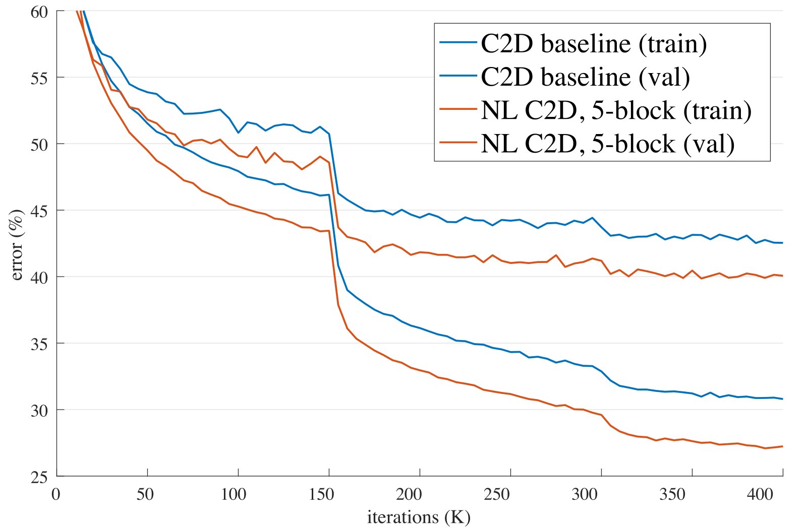
Figure 4: Curves of the training procedure on Kinetics for the ResNet-50 C2D baseline (blue) vs. non-local C2D with 5 blocks (red). We show the top-1 training error (dash) and validation error (solid). The validation error is computed in the same way as the training error (so it is 1-clip testing with the same random jittering at training time); the final results are in Table 2c (R50, 5-block).

图 4：Kinetics 上 ResNet-50 C2D 基线（蓝）与带 5 块的非局部 C2D（红）的训练曲线。虚线为 top-1 训练误差，实线为验证误差。验证误差按与训练相同方式计算（故为单片段测试，并带与训练时相同的随机抖动）；最终结果见表 2c（R50，5 块）。

5 Experiments on Video Classification

5 视频分类实验

We perform comprehensive studies on the challenging Kinetics dataset Kay2017. We also report results on the Charades dataset Sigurdsson2016 to show the generality of our models.

我们在具有挑战性的 Kinetics（Kay2017）上做系统研究，并在 Charades（Sigurdsson2016）上报结果以展示通用性。

5.1 Experiments on Kinetics

5.1 Kinetics 实验

Kinetics Kay2017 contains $\scriptstyle\sim$246k training videos and 20k validation videos. It is a classification task involving 400 human action categories. We train all models on the training set and test on the validation set.

Kinetics（Kay2017）约有 24.6 万训练视频与 2 万验证视频，是含 400 类人类动作的分类任务。所有模型在训练集上训练、在验证集上测试。

Figure 4 shows the curves of the training procedure of a ResNet-50 C2D baseline vs. a non-local C2D with 5 blocks (more details in the following). Our non-local C2D model is consistently better than the C2D baseline throughout the training procedure, in both training and validation error.

图 4 给出 ResNet-50 C2D 基线与带 5 块非局部 C2D 的训练过程曲线（细节见下）。在整个训练过程中，无论训练还是验证误差，非局部 C2D 都持续优于 C2D 基线。

Figure 1 and Figure 3 visualize several examples of the behavior of a non-local block computed by our models. Our network can learn to find meaningful relational clues regardless of the distance in space and time.

图 1 与图 3 可视化了由我们模型计算的非局部块行为的若干例子。网络能学会找到有意义的关系线索，而不论其在空间与时间上的距离。

Table 2 shows the ablation results, analyzed as follows:

表 2 给出消融结果，分析如下：

Instantiations.

Table 2a compares different types of a single non-local block added to the C2D baseline (right before the last residual block of res4). Even adding one non-local block can lead to $\scriptstyle\sim$1% improvement over the baseline.

实例化。

表 2a 比较向 C2D 基线加入单个不同类型非局部块（插在 res4 最后一个残差块之前）。即便只加一块，也可相对基线提升约 1%。

Interestingly, the embedded Gaussian, dot-product, and concatenation versions perform similarly, up to some random variations (72.7 to 72.9). As discussed in Sec. 3.2, the non-local operations with Gaussian kernels become similar to the self-attention module Vaswani2017. However, our experiments show that the attentional (softmax) behavior of this module is not the key to the improvement in our applications; instead, it is more likely that the non-local behavior is important, and it is insensitive to the instantiations.

有趣的是，嵌入高斯、点积与拼接版本表现相近，仅有随机波动（72.7 到 72.9）。如第 3.2 节所论，带高斯核的非局部运算类似于自注意力模块（Vaswani2017）。但实验表明，该模块的注意力（softmax）行为不是我们应用中提升的关键；更可能是非局部行为本身重要，且对实例化不敏感。

In the rest of this paper, we use the embedded Gaussian version by default. This version is easier to visualize as its softmax scores are in the range of $[0,1]$.

后文默认使用嵌入高斯版。该版本 softmax 分数落在 $[0,1]$，更易可视化。

Which stage to add non-local blocks?

Table 2b compares a single non-local block added to different stages of ResNet. The block is added to right before the last residual block of a stage. The improvement of a non-local block on res2, res3, or res4 is similar, and on res5 is slightly smaller. One possible explanation is that res5 has a small spatial size (7$\times$7) and it is insufficient to provide precise spatial information. More evidence of a non-local block exploiting spatial information will be investigated in Table 2d.

非局部块加在哪一阶段？

表 2b 比较单个非局部块加到 ResNet 不同阶段（加在该阶段最后一个残差块之前）。在 res2、res3 或 res4 上的提升相近，在 res5 上略小。一种解释是 res5 空间尺寸小（7$\times$7），不足以提供精确空间信息。表 2d 会进一步考察非局部块对空间信息的利用。

model	backbone	modality	top-1 val	top-5 val	top-1 test	top-5 test	avg test†
I3D in Carreira2017	Inception	RGB	72.1	90.3	71.1	89.3	80.2
2-Stream I3D in Carreira2017	Inception	RGB + flow	75.7	92.0	74.2	91.3	82.8
RGB baseline in Bian2017	Inception-ResNet-v2	RGB	73.0	90.9	-	-	-
3-stream late fusion Bian2017	Inception-ResNet-v2	RGB + flow + audio	74.9	91.6	-	-	-
3-stream LSTM Bian2017	Inception-ResNet-v2	RGB + flow + audio	77.1	93.2	-	-	-
3-stream SATT Bian2017	Inception-ResNet-v2	RGB + flow + audio	77.7	93.2	-	-	-
NL I3D [ours]	ResNet-50	RGB	76.5	92.6	-	-	-
ResNet-101	RGB	77.7	93.3	-	-	83.8

Table 3: Comparisons with state-of-the-art results in Kinetics, reported on the val and test sets. We include the Kinetics 2017 competition winner’s results Bian2017, but their best results exploited audio signals (marked in gray) so were not vision-only solutions. †: “avg” is the average of top-1 and top-5 accuracy; individual top-1 or top-5 numbers are not available from the test server at the time of submitting this manuscript.

model	backbone	modality	top-1 val	top-5 val	top-1 test	top-5 test	avg test†
I3D in Carreira2017	Inception	RGB	72.1	90.3	71.1	89.3	80.2
2-Stream I3D in Carreira2017	Inception	RGB + flow	75.7	92.0	74.2	91.3	82.8
RGB baseline in Bian2017	Inception-ResNet-v2	RGB	73.0	90.9	-	-	-
3-stream late fusion Bian2017	Inception-ResNet-v2	RGB + flow + audio	74.9	91.6	-	-	-
3-stream LSTM Bian2017	Inception-ResNet-v2	RGB + flow + audio	77.1	93.2	-	-	-
3-stream SATT Bian2017	Inception-ResNet-v2	RGB + flow + audio	77.7	93.2	-	-	-
NL I3D [ours]	ResNet-50	RGB	76.5	92.6	-	-	-
ResNet-101	RGB	77.7	93.3	-	-	83.8

表 3：Kinetics 上与当时最优结果的比较（验证集与测试集）。我们列入 Kinetics 2017 竞赛优胜者结果（Bian2017），但其最佳结果利用了音频（标灰），并非纯视觉方案。†：「avg」为 top-1 与 top-5 准确率平均；投稿时测试服务器未提供单独的 top-1/top-5。

Going deeper with non-local blocks.

Table 2c shows the results of more non-local blocks. We add 1 block (to res4), 5 blocks (3 to res4 and 2 to res3, to every other residual block), and 10 blocks (to every residual block in res3 and res4) in ResNet-50; in ResNet-101 we add them to the corresponding residual blocks. Table 2c shows that more non-local blocks in general lead to better results. We argue that multiple non-local blocks can perform long-range multi-hop communication. Messages can be delivered back and forth between distant positions in spacetime, which is hard to do via local models.

用非局部块加深。

表 2c 给出更多非局部块的结果。ResNet-50 中加 1 块（到 res4）、5 块（res4 加 3、res3 加 2，每隔一个残差块）、10 块（res3 与 res4 的每个残差块）；ResNet-101 加到对应残差块。表 2c 显示更多非局部块总体带来更好结果。我们认为多个非局部块可进行长程多跳通信：消息可在时空远距位置之间来回传递，这是局部模型难以做到的。

It is noteworthy that the improvement of non-local blocks is not just because they add depth to the baseline model. To see this, we note that in Table 2c the non-local 5-block ResNet-50 model has 73.8 accuracy, higher than the deeper ResNet-101 baseline’s 73.1. However, the 5-block ResNet-50 has only $\scriptstyle\sim$70% parameters and $\scriptstyle\sim$80% FLOPs of the ResNet-101 baseline, and is also shallower. This comparison shows that the improvement due to non-local blocks is complementary to going deeper in standard ways.

值得强调：非局部块的提升不只因为加深了基线。见表 2c，5 块非局部 ResNet-50 准确率 73.8，高于更深的 ResNet-101 基线 73.1；但前者参数量约只有后者的 70%、FLOPs 约 80%，也更浅。这说明非局部块带来的提升与按常规方式加深是互补的。

We have also tried to add standard residual blocks, instead of non-local blocks, to the baseline models. The accuracy is not increased. This again shows that the improvement of non-local blocks is not just because they add depth.

我们还试过向基线加入标准残差块而非非局部块，准确率未提升。再次说明非局部块的收益不只来自加深。

Non-local in spacetime.

Our method can naturally handle spacetime signals. This is a nice property: related objects in a video can present at distant space and long-term time interval, and their dependency can be captured by our model.

时空中的非局部。

我们的方法可自然处理时空信号。这是优点：视频中相关物体可出现在远距空间与长时间间隔，其依赖可由模型捕获。

In Table 2d we study the effect of non-local blocks applied along space, time, or spacetime. For example, in the space-only version, the non-local dependency only happens within the same frame: i.e., in Eq.(1) it only sums over the index $j$ in the same frame of the index $i$. The time-only version can be set up similarly. Table 2d shows that both the space-only and time-only versions improve over the C2D baseline, but are inferior to the spacetime version.

表 2d 研究非局部块沿空间、时间或时空施加的效果。例如，仅空间版中，非局部依赖只发生在同一帧内：即式 (1) 只对与索引 $i$ 同帧的索引 $j$ 求和。仅时间版可类似设置。表 2d 显示仅空间与仅时间版都优于 C2D 基线，但都逊于时空版。

Non-local net vs. 3D ConvNet.

Table 2e compares our non-local C2D version with the inflated 3D ConvNets. Non-local operations and 3D convolutions can be seen as two ways of extending C2D to the temporal dimensions.

非局部网络 对 3D ConvNet。

表 2e 比较非局部 C2D 与膨胀 3D ConvNet。非局部运算与 3D 卷积可视为把 C2D 扩展到时间维的两种方式。

Table 2e also compares the number of parameters and FLOPs, relative to the baseline. Our non-local C2D model is more accurate than the I3D counterpart (e.g., 75.1 vs. 74.4), while having a smaller number of FLOPs (1.2$\times$ vs. 1.5$\times$). This comparison shows that our method can be more effective than 3D convolutions when used alone.

表 2e 还比较相对基线的参数量与 FLOPs。非局部 C2D 比 I3D 对应物更准（如 75.1 对 74.4），同时 FLOPs 更少（1.2$\times$ 对 1.5$\times$）。说明单独使用时，我们的方法可比 3D 卷积更有效。

Non-local 3D ConvNet.

Despite the above comparison, non-local operations and 3D convolutions can model different aspects of the problem: 3D convolutions can capture local dependency. Table 2f shows the results of inserting 5 non-local blocks into the I3D3×1×1 models. These non-local I3D (NL I3D) models improve over their I3D counterparts (+1.6 point accuracy), showing that non-local operations and 3D convolutions are complementary.

非局部 3D ConvNet。

尽管有上述比较，非局部运算与 3D 卷积可建模问题的不同侧面：3D 卷积能捕获局部依赖。表 2f 给出向 I3D3×1×1 插入 5 个非局部块的结果。这些非局部 I3D（NL I3D）相对 I3D 对应物提升约 1.6 个百分点，说明非局部运算与 3D 卷积互补。

Longer sequences.

Finally we investigate the generality of our models on longer input videos. We use input clips consisting of 128 consecutive frames without subsampling. The sequences throughout all layers in the networks are thus 4$\times$ longer compared to the 32-frame counterparts. To fit this model into memory, we reduce the mini-batch size to 2 clips per GPU. As a result of using small mini-batches, we freeze all BN layers in this case. We initialize this model from the corresponding models trained with 32-frame inputs. We fine-tune on 128-frame inputs using the same number of iterations as the 32-frame case (though the mini-batch size is now smaller), starting with a learning rate of 0.0025. Other implementation details are the same as before.

更长序列。

最后考察模型在更长输入视频上的通用性。我们使用由连续 128 帧、不做下采样构成的输入片段。网络各层序列长度因而相对 32 帧对应物长 4 倍。为装入显存，每 GPU 小批量减为 2 个片段；因小批量较小，此时冻结所有 BN 层。模型由对应的 32 帧训练模型初始化。在 128 帧输入上用与 32 帧相同的迭代次数微调（尽管小批量更小），初始学习率 0.0025。其他实现细节同前。

Table 2g shows the results of 128-frame clips. Comparing with the 32-frame counterparts in Table 2f, all models have better results on longer inputs. We also find that our NL I3D can maintain its gain over the I3D counterparts, showing that our models work well on longer sequences.

表 2g 给出 128 帧片段结果。与表 2f 的 32 帧对应物相比，所有模型在更长输入上都更好。我们也发现 NL I3D 能相对 I3D 保持增益，说明模型在更长序列上仍表现良好。

Comparisons with state-of-the-art results.

Table 3 shows the results from the I3D authors Carreira2017 and from the Kinetics 2017 competition winner Bian2017. We note that these are comparisons of systems which can differ in many aspects. Nevertheless, our method surpasses all the existing RGB or RGB + flow based methods by a good margin. Without using optical flow and without any bells and whistles, our method is on par with the heavily engineered results of the 2017 competition winner.

与当时最优结果比较。

表 3 给出 I3D 作者（Carreira2017）与 Kinetics 2017 竞赛优胜者（Bian2017）的结果。需注意这是可能在多方面不同的系统之间的比较。尽管如此，我们的方法以较大优势超过所有既有 RGB 或 RGB+光流方法。不用光流、不加花哨技巧，方法与 2017 竞赛优胜者经大量工程打磨的结果持平。

model	modality	train/val	trainval/test
2-Stream Sigurdsson2017	RGB + flow	18.6	-
2-Stream +LSTM Sigurdsson2017	RGB + flow	17.8	-
Asyn-TF Sigurdsson2017	RGB + flow	22.4	-
I3D Carreira2017	RGB	32.9	34.4
I3D [ours]	RGB	35.5	37.2
NL I3D [ours]	RGB	37.5	39.5

Table 4: Classification mAP (%) in the Charades dataset Sigurdsson2016, on the train/val split and the trainval/test split. Our results are based on ResNet-101. Our NL I3D uses 5 non-local blocks.

model	modality	train/val	trainval/test
2-Stream Sigurdsson2017	RGB + flow	18.6	-
2-Stream +LSTM Sigurdsson2017	RGB + flow	17.8	-
Asyn-TF Sigurdsson2017	RGB + flow	22.4	-
I3D Carreira2017	RGB	32.9	34.4
I3D [ours]	RGB	35.5	37.2
NL I3D [ours]	RGB	37.5	39.5

表 4：Charades 数据集（Sigurdsson2016）上的分类 mAP（%），分别在 train/val 与 trainval/test 划分上。我们的结果基于 ResNet-101。NL I3D 使用 5 个非局部块。

5.2 Experiments on Charades

5.2 Charades 实验

Charades Sigurdsson2016 is a video dataset with $\scriptstyle\sim$8k training, $\scriptstyle\sim$1.8k validation, and $\scriptstyle\sim$2k testing videos. It is a multi-label classification task with 157 action categories. We use a per-category sigmoid output to handle the multi-label property.

Charades（Sigurdsson2016）约有 8k 训练、1.8k 验证与 2k 测试视频，是含 157 个动作类的多标签分类。我们用逐类 sigmoid 输出处理多标签。

We initialize our models pre-trained on Kinetics (128-frame). The mini-batch size is set to 1 clip per GPU. We train our models for 200k iterations, starting from a learning rate of 0.00125 and reducing it by 10 every 75k iterations. We use a jittering strategy similar to that in Kinetics to determine the location of the 224$\times$224 cropping window, but we rescale the video such that this cropping window outputs 288$\times$288 pixels, on which we fine-tune our network. We test on a single scale of 320 pixels.

用在 Kinetics（128 帧）上预训练的模型初始化。每 GPU 小批量设为 1 个片段。训练 200k 迭代，初始学习率 0.00125，每 75k 迭代降 10 倍。裁剪窗口位置的抖动策略类似 Kinetics，但把视频缩放使该 224$\times$224 裁剪窗输出 288$\times$288 像素，再在其上微调。测试使用单尺度 320 像素。

Table 4 shows the comparisons with the previous results on Charades. The result of Carreira2017 is the 2017 competition winner in Charades, which was also fine-tuned from models pre-trained in Kinetics. Our I3D baseline is higher than previous results. As a controlled comparison, our non-local net improves over our I3D baseline by 2.3% on the test set.

表 4 给出与 Charades 既往结果的比较。Carreira2017 的结果是 Charades 2017 竞赛优胜者，同样从 Kinetics 预训练模型微调。我们的 I3D 基线高于既往结果。作为受控比较，非局部网络在测试集上相对我们的 I3D 基线提升 2.3%。

6 Extension: Experiments on COCO

6 扩展：COCO 实验

We also investigate our models on static image recognition. We experiment on the Mask R-CNN baseline He2017 for COCO Lin2014 object detection/segmentation and human pose estimation (keypoint detection). The models are trained on COCO train2017 (i.e., trainval35k in 2014) and tested on val2017 (i.e., minival in 2014).

我们也在静态图像识别上考察模型。实验基于 Mask R-CNN 基线（He2017），任务为 COCO（Lin2014）目标检测/分割与人体姿态估计（关键点检测）。模型在 COCO train2017（即 2014 的 trainval35k）上训练，在 val2017（即 2014 的 minival）上测试。

Object detection and instance segmentation.

We modify the Mask R-CNN backbone by adding one non-local block (right before the last residual block of res4). All models are fine-tuned from ImageNet pre-training. We evaluate on a standard baseline of ResNet-50/101 and a high baseline of ResNeXt-152 (X152) Xie2017. Unlike the original paper He2017 that adopted stage-wise training regarding RPN, we use an improved implementation with end-to-end joint training similar to Ren2017, which leads to higher baselines than He2017.

目标检测与实例分割。

我们修改 Mask R-CNN 骨干：在 res4 最后一个残差块前加入一个非局部块。所有模型从 ImageNet 预训练微调。评估标准基线 ResNet-50/101，以及更高基线 ResNeXt-152（X152，Xie2017）。与原论文 He2017 对 RPN 分阶段训练不同，我们采用类似 Ren2017 的端到端联合训练改进实现，基线高于 He2017。

Table 5 shows the box and mask AP on COCO. We see that a single non-local block improves all R50/101 and X152 baselines, on all metrics involving detection and segmentation. AP${}^{\text{box}}$ is increased by $\scriptstyle\sim$1 point in all cases (e.g., +1.3 point in R101). Our non-local block is complementary to increasing the model capacity, even when the model is upgraded from R50/101 to X152. This comparison suggests that non-local dependency has not been sufficiently captured by existing models despite increased depth/capacity.

表 5 给出 COCO 上的框与掩码 AP。单个非局部块在所有 R50/101 与 X152 基线上、在检测与分割相关的所有指标上都有提升。AP${}^{\text{box}}$ 在所有情形下约提高 1 点（如 R101 上 +1.3）。即便模型从 R50/101 升到 X152，非局部块仍与增大容量互补。这表明尽管深度/容量增加，既有模型仍未充分捕获非局部依赖。

In addition, the above gain is at a very small cost. The single non-local block only adds $<$5% computation to the baseline model. We also have tried to use more non-local blocks to the backbone, but found diminishing return.

此外，上述收益代价很小：单个非局部块相对基线只增加不到 5% 计算量。我们也试过在骨干中使用更多非局部块，但收益递减。

method	AP${}^{\text{box}}$	AP${}^{\text{box}}_{50}$	AP${}^{\text{box}}_{75}$	AP${}^{\text{mask}}$	AP${}^{\text{mask}}_{50}$	AP${}^{\text{mask}}_{75}$
R50	baseline	38.0	59.6	41.0	34.6	56.4	36.5
+1 NL	39.0	61.1	41.9	35.5	58.0	37.4
R101	baseline	39.5	61.4	42.9	36.0	58.1	38.3
+1 NL	40.8	63.1	44.5	37.1	59.9	39.2
X152	baseline	44.1	66.4	48.4	39.7	63.2	42.2
+1 NL	45.0	67.8	48.9	40.3	64.4	42.8

Table 5: Adding 1 non-local block to Mask R-CNN for COCO object detection and instance segmentation. The backbone is ResNet-50/101 or ResNeXt-152 Xie2017, both with FPN Lin2017.

method	AP${}^{\text{box}}$	AP${}^{\text{box}}_{50}$	AP${}^{\text{box}}_{75}$	AP${}^{\text{mask}}$	AP${}^{\text{mask}}_{50}$	AP${}^{\text{mask}}_{75}$
R50	baseline	38.0	59.6	41.0	34.6	56.4	36.5
+1 NL	39.0	61.1	41.9	35.5	58.0	37.4
R101	baseline	39.5	61.4	42.9	36.0	58.1	38.3
+1 NL	40.8	63.1	44.5	37.1	59.9	39.2
X152	baseline	44.1	66.4	48.4	39.7	63.2	42.2
+1 NL	45.0	67.8	48.9	40.3	64.4	42.8

表 5：向 Mask R-CNN 加入 1 个非局部块用于 COCO 目标检测与实例分割。骨干为带 FPN（Lin2017）的 ResNet-50/101 或 ResNeXt-152（Xie2017）。

Keypoint detection.

Next we evaluate non-local blocks in Mask R-CNN for keypoint detection. In He2017, Mask R-CNN used a stack of 8 convolutional layers for predicting the keypoints as 1-hot masks. These layers are local operations and may overlook the dependency among keypoints across long distance. Motivated by this, we insert 4 non-local blocks into the keypoint head (after every 2 convolutional layers).

关键点检测。

接下来在 Mask R-CNN 的关键点检测中评估非局部块。He2017 中，Mask R-CNN 用 8 层卷积堆叠把关键点预测为一热掩码。这些层是局部运算，可能忽视远距关键点之间的依赖。受此启发，我们向关键点头插入 4 个非局部块（每 2 个卷积层后插入一个）。

Table 6 shows the results on COCO. On a strong baseline of R101, adding 4 non-local blocks to the keypoint head leads to a $\scriptstyle\sim$1 point increase of keypoint AP. If we add one extra non-local block to the backbone as done for object detection, we observe an in total 1.4 points increase of keypoint AP over the baseline. In particular, we see that the stricter criterion of AP75 is boosted by 2.4 points, suggesting a stronger localization performance.

表 6 给出 COCO 结果。在强 R101 基线上，向关键点头加 4 个非局部块约提升 1 点关键点 AP。若再像目标检测那样向骨干额外加 1 个非局部块，关键点 AP 相对基线总共提升 1.4 点。尤其更严的 AP75 提升 2.4 点，表明定位更强。

model	AP${}^{\text{kp}}$	AP${}^{\text{kp}}_{50}$	AP${}^{\text{kp}}_{75}$
R101 baseline	65.1	86.8	70.4
NL, +4 in head	66.0	87.1	71.7
NL, +4 in head, +1 in backbone	66.5	87.3	72.8

Table 6: Adding non-local blocks to Mask R-CNN for COCO keypoint detection. The backbone is ResNet-101 with FPN Lin2017.

model	AP${}^{\text{kp}}$	AP${}^{\text{kp}}_{50}$	AP${}^{\text{kp}}_{75}$
R101 baseline	65.1	86.8	70.4
NL, +4 in head	66.0	87.1	71.7
NL, +4 in head, +1 in backbone	66.5	87.3	72.8

表 6：向 Mask R-CNN 加入非局部块用于 COCO 关键点检测。骨干为带 FPN（Lin2017）的 ResNet-101。

7 Conclusion

7 结论

We presented a new class of neural networks which capture long-range dependencies via non-local operations. Our non-local blocks can be combined with any existing architectures. We show the significance of non-local modeling for the tasks of video classification, object detection and segmentation, and pose estimation. On all tasks, a simple addition of non-local blocks provides solid improvement over baselines. We hope non-local layers will become an important component of future network architectures.

我们提出一类通过非局部运算捕获长程依赖的神经网络。非局部块可与任意既有结构组合。我们展示了非局部建模对视频分类、目标检测与分割、以及姿态估计的重要性。在所有任务上，简单加入非局部块都能相对基线带来扎实提升。希望非局部层成为未来网络结构的重要组件。

Acknowledgement: This work was partially supported by ONR MURI N000141612007, Sloan, Okawa Fellowship to AG and NVIDIA Fellowship to XW. We would also like to thank Haoqi Fan, Du Tran, Heng Wang, Georgia Gkioxari and Piotr Dollar for many helpful discussions.

致谢：本工作部分得到 ONR MURI N000141612007、Sloan、AG 的 Okawa Fellowship 以及 XW 的 NVIDIA Fellowship 支持。感谢 Haoqi Fan、Du Tran、Heng Wang、Georgia Gkioxari 与 Piotr Dollar 的诸多有益讨论。

References

参考文献

(1) C. Barnes, E. Shechtman, A. Finkelstein, and D. B. Goldman. Patchmatch: A randomized correspondence algorithm for structural image editing. In Proceedings of SIGGRAPH, ACM Transactions on Graphics , 2009.

(2) P. Battaglia, R. Pascanu, M. Lai, D. J. Rezende, et al. Interaction networks for learning about objects, relations and physics. In Neural Information Processing Systems (NIPS) , 2016.

(3) Y. Bian, C. Gan, X. Liu, F. Li, X. Long, Y. Li, H. Qi, J. Zhou, S. Wen, and Y. Lin. Revisiting the effectiveness of off-the-shelf temporal modeling approaches for large-scale video classification. arXiv:1708.03805 , 2017.

(4) A. Buades, B. Coll, and J.-M. Morel. A non-local algorithm for image denoising. In Computer Vision and Pattern Recognition (CVPR) , 2005.

(5) H. C. Burger, C. J. Schuler, and S. Harmeling. Image denoising: Can plain neural networks compete with BM3D? In Computer Vision and Pattern Recognition (CVPR) , 2012.

(6) H. C. Burger, C. J. Schuler, and S. Harmeling. Image denoising with multi-layer perceptrons, part 2: training trade-offs and analysis of their mechanisms. arXiv:1211.1552 , 2012.

(7) J. Carreira and A. Zisserman. Quo vadis, action recognition? a new model and the kinetics dataset. In Computer Vision and Pattern Recognition (CVPR) , 2017.

(8) S. Chandra, N. Usunier, and I. Kokkinos. Dense and low-rank Gaussian CRFs using deep embeddings. In International Conference on Computer Vision (ICCV) , 2017.

(9) L.-C. Chen, G. Papandreou, I. Kokkinos, K. Murphy, and A. L. Yuille. Semantic image segmentation with deep convolutional nets and fully connected CRFs. arXiv:1412.7062 , 2014.

(10) K. Dabov, A. Foi, V. Katkovnik, and K. Egiazarian. Image denoising by sparse 3-d transform-domain collaborative filtering. Transactions on Image Processing (TIP) , 2007.

(11) J. Donahue, L. Anne Hendricks, S. Guadarrama, M. Rohrbach, S. Venugopalan, K. Saenko, and T. Darrell. Long-term recurrent convolutional networks for visual recognition and description. In Computer Vision and Pattern Recognition (CVPR) , 2015.

(12) A. A. Efros and T. K. Leung. Texture synthesis by non-parametric sampling. In International Conference on Computer Vision (ICCV) , 1999.

(13) C. Feichtenhofer, A. Pinz, and R. Wildes. Spatiotemporal residual networks for video action recognition. In Neural Information Processing Systems (NIPS) , 2016.

(14) K. Fukushima and S. Miyake. Neocognitron: A self-organizing neural network model for a mechanism of visual pattern recognition. In Competition and cooperation in neural nets . Springer, 1982.

(15) J. Gehring, M. Auli, D. Grangier, D. Yarats, and Y. N. Dauphin. Convolutional sequence to sequence learning. In International Conference on Machine Learning (ICML) , 2017.

(16) D. Glasner, S. Bagon, and M. Irani. Super-resolution from a single image. In Computer Vision and Pattern Recognition (CVPR) , 2009.

(17) P. Goyal, P. Dollár, R. Girshick, P. Noordhuis, L. Wesolowski, A. Kyrola, A. Tulloch, Y. Jia, and K. He. Accurate, large minibatch sgd: Training imagenet in 1 hour. arXiv:1706.02677 , 2017.

(18) A. Harley, K. Derpanis, and I. Kokkinos. Segmentation-aware convolutional networks using local attention masks. In International Conference on Computer Vision (ICCV) , 2017.

(19) K. He, G. Gkioxari, P. Dollár, and R. Girshick. Mask R-CNN. In International Conference on Computer Vision (ICCV) , 2017.

(20) K. He, X. Zhang, S. Ren, and J. Sun. Delving deep into rectifiers: Surpassing human-level performance on imagenet classification. In International Conference on Computer Vision (ICCV) , 2015.

(21) K. He, X. Zhang, S. Ren, and J. Sun. Deep residual learning for image recognition. In Computer Vision and Pattern Recognition (CVPR) , 2016.

(22) G. E. Hinton, N. Srivastava, A. Krizhevsky, I. Sutskever, and R. R. Salakhutdinov. Improving neural networks by preventing co-adaptation of feature detectors. arXiv:1207.0580 , 2012.

(23) S. Hochreiter and J. Schmidhuber. Long short-term memory. Neural computation , 1997.

(24) Y. Hoshen. Multi-agent predictive modeling with attentional commnets. In Neural Information Processing Systems (NIPS) , 2017.

(25) S. Ioffe and C. Szegedy. Batch normalization: Accelerating deep network training by reducing internal covariate shift. In International Conference on Machine Learning (ICML) , 2015.

(26) S. Ji, W. Xu, M. Yang, and K. Yu. 3d convolutional neural networks for human action recognition. In International Conference on Machine Learning (ICML) , 2010.

(27) W. Kay, J. Carreira, K. Simonyan, B. Zhang, C. Hillier, S. Vijayanarasimhan, F. Viola, T. Green, T. Back, P. Natsev, et al. The kinetics human action video dataset. arXiv:1705.06950 , 2017.

(28) P. Krähenbühl and V. Koltun. Efficient inference in fully connected crfs with gaussian edge potentials. In Neural Information Processing Systems (NIPS) , 2011.

(29) J. Lafferty, A. McCallum, and F. C. Pereira. Conditional random fields: Probabilistic models for segmenting and labeling sequence data. In International Conference on Machine Learning (ICML) , 2001.

(30) Y. LeCun, B. Boser, J. S. Denker, D. Henderson, R. E. Howard, W. Hubbard, and L. D. Jackel. Backpropagation applied to handwritten zip code recognition. Neural computation , 1989.

(31) S. Lefkimmiatis. Non-local color image denoising with convolutional neural networks. In Computer Vision and Pattern Recognition (CVPR) , 2017.

(32) T.-Y. Lin, P. Dollár, R. Girshick, K. He, B. Hariharan, and S. Belongie. Feature pyramid networks for object detection. In Computer Vision and Pattern Recognition (CVPR) , 2017.

(33) T.-Y. Lin, M. Maire, S. Belongie, J. Hays, P. Perona, D. Ramanan, P. Dollár, and C. L. Zitnick. Microsoft COCO: Common objects in context. In European Conference on Computer Vision (ECCV) . 2014.

(34) S. Liu, S. De Mello, J. Gu, G. Zhong, M.-H. Yang, and J. Kautz. Learning affinity via spatial propagation networks. In Neural Information Processing Systems (NIPS) , 2017.

(35) V. Nair and G. E. Hinton. Rectified linear units improve restricted boltzmann machines. In International Conference on Machine Learning (ICML) , 2010.

(36) A. Oord, S. Dieleman, H. Zen, K. Simonyan, O. Vinyals, A. Graves, N. Kalchbrenner, A. Senior, and K. Kavukcuoglu. Wavenet: A generative model for raw audio. arXiv:1609.03499 , 2016.

(37) S. Ren, K. He, R. Girshick, and J. Sun. Faster R-CNN: Towards real-time object detection with region proposal networks. Transactions on Pattern Analysis and Machine Intelligence (TPAMI) , 2017.

(38) D. E. Rumelhart, G. E. Hinton, and R. J. Williams. Learning representations by back-propagating errors. Nature , 1986.

(39) O. Russakovsky, J. Deng, H. Su, J. Krause, S. Satheesh, S. Ma, Z. Huang, A. Karpathy, A. Khosla, M. Bernstein, A. C. Berg, and L. Fei-Fei. ImageNet Large Scale Visual Recognition Challenge. International Journal of Computer Vision (IJCV) , 2015.

(40) A. Santoro, D. Raposo, D. G. Barrett, M. Malinowski, R. Pascanu, P. Battaglia, and T. Lillicrap. A simple neural network module for relational reasoning. In Neural Information Processing Systems (NIPS) , 2017.

(41) F. Scarselli, M. Gori, A. C. Tsoi, M. Hagenbuchner, and G. Monfardini. The graph neural network model. IEEE Transactions on Neural Networks , 2009.

(42) A. G. Schwing and R. Urtasun. Fully connected deep structured networks. arXiv preprint arXiv:1503.02351 , 2015.

(43) G. A. Sigurdsson, S. Divvala, A. Farhadi, and A. Gupta. Asynchronous temporal fields for action recognition. In Computer Vision and Pattern Recognition (CVPR) , 2017.

(44) G. A. Sigurdsson, G. Varol, X. Wang, A. Farhadi, I. Laptev, and A. Gupta. Hollywood in homes: Crowdsourcing data collection for activity understanding. In European Conference on Computer Vision (ECCV) , 2016.

(45) K. Simonyan and A. Zisserman. Two-stream convolutional networks for action recognition in videos. In Neural Information Processing Systems (NIPS) , 2014.

(46) K. Simonyan and A. Zisserman. Very deep convolutional networks for large-scale image recognition. In International Conference on Learning Representations (ICLR) , 2015.

(47) C. Tomasi and R. Manduchi. Bilateral filtering for gray and color images. In International Conference on Computer Vision (ICCV) , 1998.

(48) D. Tran, L. Bourdev, R. Fergus, L. Torresani, and M. Paluri. Learning spatiotemporal features with 3d convolutional networks. In International Conference on Computer Vision (ICCV) , 2015.

(49) A. Vaswani, N. Shazeer, N. Parmar, J. Uszkoreit, L. Jones, A. N. Gomez, L. Kaiser, and I. Polosukhin. Attention is all you need. In Neural Information Processing Systems (NIPS) , 2017.

(50) H. Wang and C. Schmid. Action recognition with improved trajectories. In International Conference on Computer Vision (ICCV) , 2013.

(51) L. Wang, Y. Qiao, and X. Tang. Action recognition with trajectory-pooled deep-convolutional descriptors. In Computer Vision and Pattern Recognition (CVPR) , 2015.

(52) N. Watters, A. Tacchetti, T. Weber, R. Pascanu, P. Battaglia, and D. Zoran. Visual interaction networks. In Neural Information Processing Systems (NIPS) , 2017.

(53) S. Xie, R. Girshick, P. Dollár, Z. Tu, and K. He. Aggregated residual transformations for deep neural networks. In Computer Vision and Pattern Recognition (CVPR) , 2017.

(54) W. Xiong, J. Droppo, X. Huang, F. Seide, M. Seltzer, A. Stolcke, D. Yu, and G. Zweig. The Microsoft 2016 Conversational Speech Recognition System. In International Conference on Acoustics, Speech, and Signal Processing (ICASSP) , 2017.

(55) J. Yue-Hei Ng, M. Hausknecht, S. Vijayanarasimhan, O. Vinyals, R. Monga, and G. Toderici. Beyond short snippets: Deep networks for video classification. In Computer Vision and Pattern Recognition (CVPR) , 2015.

(56) S. Zheng, S. Jayasumana, B. Romera-Paredes, V. Vineet, Z. Su, D. Du, C. Huang, and P. H. Torr. Conditional random fields as recurrent neural networks. In International Conference on Computer Vision (ICCV) , 2015.