node2vec: Scalable Feature Learning for Networks
ISBN 978-1-4503-4232-2/16/08. DOI: http://dx.doi.org/10.1145/2939672.2939754
ISBN 978-1-4503-4232-2/16/08。DOI:http://dx.doi.org/10.1145/2939672.2939754
node2vec: Scalable Feature Learning for Networks
Aditya Grover Jure Leskovec Address: Stanford University Email: adityag@cs.stanford.edu Address: Stanford University Email: jure@cs.stanford.edu
Abstract
摘要
Prediction tasks over nodes and edges in networks require careful effort in engineering features used by learning algorithms. Recent research in the broader field of representation learning has led to significant progress in automating prediction by learning the features themselves. However, present feature learning approaches are not expressive enough to capture the diversity of connectivity patterns observed in networks.
网络中关于节点和边的预测任务,需要仔细为学习算法构造所用的特征。表征学习这一更广领域的近期研究,已经通过让模型自己学习特征,在自动完成预测上取得了显著进展。不过,现有的特征学习方法还不够有表达力,难以刻画网络中观察到的多样化连接模式。
Here we propose node2vec, an algorithmic framework for learning continuous feature representations for nodes in networks. In node2vec, we learn a mapping of nodes to a low-dimensional space of features that maximizes the likelihood of preserving network neighborhoods of nodes. We define a flexible notion of a node’s network neighborhood and design a biased random walk procedure, which efficiently explores diverse neighborhoods. Our algorithm generalizes prior work which is based on rigid notions of network neighborhoods, and we argue that the added flexibility in exploring neighborhoods is the key to learning richer representations.
本文提出 node2vec,一套为网络中的节点学习连续特征表示的算法框架。在 node2vec 中,我们学习一个把节点映射到低维特征空间的映射,使保住节点网络邻域的似然最大化。我们定义了一种灵活的节点网络邻域概念,并设计了一种带偏置的随机游走过程,能够高效地探索多样化的邻域。我们的算法推广了先前基于僵硬邻域定义的工作;我们认为,探索邻域时增加的灵活性,是学到更丰富表示的关键。
We demonstrate the efficacy of node2vec over existing state-of-the-art techniques on multi-label classification and link prediction in several real-world networks from diverse domains. Taken together, our work represents a new way for efficiently learning state-of-the-art task-independent representations in complex networks.
我们在来自不同领域的若干真实网络上,用多标签分类和链接预测展示了 node2vec 相对当时最好技术的有效性。综合来看,这项工作提供了一种在复杂网络中高效学习与任务无关、且达到当时最好水平的表示的新途径。
Categories and Subject Descriptors: H.2.8 [Database Management]: Database applications—Data mining; I.2.6 [Artificial Intelligence]: Learning
分类与主题描述符: H.2.8 [数据库管理]:数据库应用—数据挖掘;I.2.6 [人工智能]:学习
General Terms: Algorithms; Experimentation.
一般术语: 算法;实验。
Keywords: Information networks, Feature learning, Node embeddings, Graph representations.
关键词: 信息网络,特征学习,节点嵌入,图表示。
1 Introduction
1 引言
Many important tasks in network analysis involve predictions over nodes and edges. In a typical node classification task, we are interested in predicting the most probable labels of nodes in a network [33]. For example, in a social network, we might be interested in predicting interests of users, or in a protein-protein interaction network we might be interested in predicting functional labels of proteins [25, 37]. Similarly, in link prediction, we wish to predict whether a pair of nodes in a network should have an edge connecting them [18]. Link prediction is useful in a wide variety of domains; for instance, in genomics, it helps us discover novel interactions between genes, and in social networks, it can identify real-world friends [2, 34].
网络分析中许多重要任务,都涉及对节点和边做预测。在典型的节点分类任务中,我们希望预测网络中节点最可能的标签 [33]。例如,在社交网络中,我们可能想预测用户的兴趣;在蛋白质相互作用网络中,则可能想预测蛋白质的功能标签 [25, 37]。类似地,在链接预测中,我们希望预测网络中的一对节点之间是否应当有一条边相连 [18]。链接预测在许多领域都有用:例如在基因组学中,它帮助发现基因之间新的相互作用;在社交网络中,它可以识别现实世界中的朋友关系 [2, 34]。
Any supervised machine learning algorithm requires a set of informative, discriminating, and independent features. In prediction problems on networks this means that one has to construct a feature vector representation for the nodes and edges. A typical solution involves hand-engineering domain-specific features based on expert knowledge. Even if one discounts the tedious effort required for feature engineering, such features are usually designed for specific tasks and do not generalize across different prediction tasks.
任何监督机器学习算法都需要一组有信息量、有区分力且相互独立的特征。在网络上的预测问题中,这意味着必须为节点和边构造特征向量表示。典型做法是根据专家知识,手工设计领域特定的特征。即便不考虑特征工程本身的繁琐,这类特征通常也是为特定任务设计的,并不能推广到不同的预测任务上。
An alternative approach is to learn feature representations by solving an optimization problem [4]. The challenge in feature learning is defining an objective function, which involves a trade-off in balancing computational efficiency and predictive accuracy. On one side of the spectrum, one could directly aim to find a feature representation that optimizes performance of a downstream prediction task. While this supervised procedure results in good accuracy, it comes at the cost of high training time complexity due to a blowup in the number of parameters that need to be estimated. At the other extreme, the objective function can be defined to be independent of the downstream prediction task and the representations can be learned in a purely unsupervised way. This makes the optimization computationally efficient and with a carefully designed objective, it results in task-independent features that closely match task-specific approaches in predictive accuracy [21, 23].
另一种做法是通过求解一个优化问题来学习特征表示 [4]。特征学习的难点在于定义目标函数,其中需要在计算效率和预测精度之间权衡。光谱的一端,可以直接寻找能优化下游预测任务性能的特征表示。这种有监督的程序精度不错,但需要估计的参数数量会急剧增加,训练时间复杂度很高。光谱的另一端,可以把目标函数定义成与下游预测任务无关,并以完全无监督的方式学习表示。这样优化在计算上更高效;若目标设计得当,得到的与任务无关的特征,在预测精度上可以接近任务特定的方法 [21, 23]。
However, current techniques fail to satisfactorily define and optimize a reasonable objective required for scalable unsupervised feature learning in networks. Classic approaches based on linear and non-linear dimensionality reduction techniques such as Principal Component Analysis, Multi-Dimensional Scaling and their extensions [3, 27, 30, 35] optimize an objective that transforms a representative data matrix of the network such that it maximizes the variance of the data representation. Consequently, these approaches invariably involve eigendecomposition of the appropriate data matrix which is expensive for large real-world networks. Moreover, the resulting latent representations give poor performance on various prediction tasks over networks.
然而,现有技术还不能令人满意地定义并优化一个合理的目标,以在网络上做可扩展的无监督特征学习。基于线性和非线性降维的经典方法,例如主成分分析、多维尺度分析及其扩展 [3, 27, 30, 35],优化的目标是变换网络的一个代表性数据矩阵,使数据表示的方差最大。因此,这些方法几乎总是需要对相应数据矩阵做特征分解,这对大规模真实网络来说代价很高。此外,得到的潜在表示在各种网络预测任务上的表现也较差。
Alternatively, we can design an objective that seeks to preserve local neighborhoods of nodes. The objective can be efficiently optimized using stochastic gradient descent (SGD) akin to backpropogation on just single hidden-layer feedforward neural networks. Recent attempts in this direction [24, 28] propose efficient algorithms but rely on a rigid notion of a network neighborhood, which results in these approaches being largely insensitive to connectivity patterns unique to networks. Specifically, nodes in networks could be organized based on communities they belong to (i.e., homophily); in other cases, the organization could be based on the structural roles of nodes in the network (i.e., structural equivalence) [7, 10, 36]. For instance, in Figure 1, we observe nodes and belonging to the same tightly knit community of nodes, while the nodes and in the two distinct communities share the same structural role of a hub node. Real-world networks commonly exhibit a mixture of such equivalences. Thus, it is essential to allow for a flexible algorithm that can learn node representations obeying both principles: ability to learn representations that embed nodes from the same network community closely together, as well as to learn representations where nodes that share similar roles have similar embeddings. This would allow feature learning algorithms to generalize across a wide variety of domains and prediction tasks.
另一种做法是设计一个力求保住节点局部邻域的目标。该目标可以用随机梯度下降(SGD)高效优化,类似于只含单隐层的前馈网络上的反向传播。这一方向上的近期尝试 [24, 28] 提出了高效算法,但依赖一种僵硬的网络邻域定义,因而对这些方法而言,网络所特有的连接模式在很大程度上是不敏感的。具体来说,网络中的节点可以按其所属社区来组织(即同配性);在另一些情形下,组织方式也可以基于节点在网络中的结构角色(即结构等价) [7, 10, 36]。例如在图 1 中,可以看到节点 和 同属一个联系紧密的节点社区,而分属两个不同社区的 和 却共享枢纽节点这一结构角色。真实网络通常会同时表现出这类等价性的混合。因此,有必要允许一种灵活的算法,使学到的节点表示同时服从这两条原则:既要把同一网络社区中的节点嵌入得靠近,也要让角色相似的节点具有相似的嵌入。这样,特征学习算法才能推广到多种多样的领域和预测任务上。
Present work. We propose node2vec, a semi-supervised algorithm for scalable feature learning in networks. We optimize a custom graph-based objective function using SGD motivated by prior work on natural language processing [21]. Intuitively, our approach returns feature representations that maximize the likelihood of preserving network neighborhoods of nodes in a -dimensional feature space. We use a 2 order random walk approach to generate (sample) network neighborhoods for nodes.
本项工作。 我们提出 node2vec,一种用于网络中可扩展特征学习的半监督算法。我们用 SGD 优化一个专门的、基于图的目标函数,其动机来自自然语言处理中的先前工作 [21]。直观上,我们的方法返回的特征表示,在 维特征空间中最大化保住节点网络邻域的似然。我们使用二阶随机游走来为节点生成(抽样)网络邻域。
Our key contribution is in defining a flexible notion of a node’s network neighborhood. By choosing an appropriate notion of a neighborhood, node2vec can learn representations that organize nodes based on their network roles and/or communities they belong to. We achieve this by developing a family of biased random walks, which efficiently explore diverse neighborhoods of a given node. The resulting algorithm is flexible, giving us control over the search space through tunable parameters, in contrast to rigid search procedures in prior work [24, 28]. Consequently, our method generalizes prior work and can model the full spectrum of equivalences observed in networks. The parameters governing our search strategy have an intuitive interpretation and bias the walk towards different network exploration strategies. These parameters can also be learned directly using a tiny fraction of labeled data in a semi-supervised fashion.
我们的关键贡献,在于定义了一种灵活的节点网络邻域概念。通过选择合适的邻域定义,node2vec 可以学到按网络角色和/或其所属社区来组织节点的表示。我们通过发展一族带偏置的随机游走来做到这一点,它们能高效地探索给定节点的多样化邻域。得到的算法是灵活的,可以通过可调参数控制搜索空间,这与先前工作中僵硬的搜索程序形成对比 [24, 28]。因此,我们的方法推广了先前工作,并能刻画网络中观察到的全部等价性谱系。支配搜索策略的参数具有直观解释,并使游走向不同的网络探索策略偏置。这些参数也可以在半监督方式下,直接用一小部分带标签数据来学习。
We also show how feature representations of individual nodes can be extended to pairs of nodes (i.e., edges). In order to generate feature representations of edges, we compose the learned feature representations of the individual nodes using simple binary operators. This compositionality lends node2vec to prediction tasks involving nodes as well as edges.
我们还说明了如何把单个节点的特征表示扩展到节点对(即边)。为了生成边的特征表示,我们用简单的二元算子组合各个节点已学到的特征表示。这种可组合性使 node2vec 既能用于涉及节点的预测任务,也能用于涉及边的预测任务。
Our experiments focus on two common prediction tasks in networks: a multi-label classification task, where every node is assigned one or more class labels and a link prediction task, where we predict the existence of an edge given a pair of nodes. We contrast the performance of node2vec with state-of-the-art feature learning algorithms [24, 28]. We experiment with several real-world networks from diverse domains, such as social networks, information networks, as well as networks from systems biology. Experiments demonstrate that node2vec outperforms state-of-the-art methods by up to 26.7% on multi-label classification and up to 12.6% on link prediction. The algorithm shows competitive performance with even 10% labeled data and is also robust to perturbations in the form of noisy or missing edges. Computationally, the major phases of node2vec are trivially parallelizable, and it can scale to large networks with millions of nodes in a few hours.
我们的实验聚焦于网络中两类常见的预测任务:多标签分类,即每个节点被赋予一个或多个类别标签;以及链接预测,即给定一对节点,预测它们之间是否存在一条边。我们把 node2vec 的表现与当时最好的特征学习算法相对照 [24, 28]。实验使用来自不同领域的若干真实网络,例如社交网络、信息网络以及系统生物学中的网络。实验表明,node2vec 相对当时最好的方法,在多标签分类上最多高出 26.7%,在链接预测上最多高出 12.6%。即使只有 10% 的带标签数据,算法也有有竞争力的表现,并且对噪声边或缺失边这类扰动也较稳健。从计算上看,node2vec 的主要阶段都可以平凡地并行化,并能在数小时内扩展到有数百万节点的大型网络。
Overall our paper makes the following contributions:
总的来说,本文做出了如下贡献:
- We propose node2vec, an efficient scalable algorithm for feature learning in networks that efficiently optimizes a novel network-aware, neighborhood preserving objective using SGD.
- 我们提出 node2vec,一种高效、可扩展的网络特征学习算法,它用 SGD 高效地优化一个新颖的、感知网络并保住邻域的目标。
- We show how node2vec is in accordance with established principles in network science, providing flexibility in discovering representations conforming to different equivalences.
- 我们说明 node2vec 与网络科学中的既有原则相一致,为发现符合不同等价性的表示提供了灵活性。
- We extend node2vec and other feature learning methods based on neighborhood preserving objectives, from nodes to pairs of nodes for edge-based prediction tasks.
- 我们把 node2vec 以及其他基于保住邻域目标的特征学习方法,从节点扩展到节点对,以服务于基于边的预测任务。
- We empirically evaluate node2vec for multi-label classification and link prediction on several real-world datasets.
- 我们在若干真实数据集上,对 node2vec 做了多标签分类和链接预测的经验评估。
The rest of the paper is structured as follows. In Section 2, we briefly survey related work in feature learning for networks. We present the technical details for feature learning using node2vec in Section 3. In Section 4, we empirically evaluate node2vec on prediction tasks over nodes and edges on various real-world networks and assess the parameter sensitivity, perturbation analysis, and scalability aspects of our algorithm. We conclude with a discussion of the node2vec framework and highlight some promising directions for future work in Section 5. Datasets and a reference implementation of node2vec are available on the project page: http://snap.stanford.edu/node2vec.
论文其余部分组织如下。第 2 节简要回顾网络特征学习的相关工作。第 3 节给出用 node2vec 做特征学习的技术细节。第 4 节在各种真实网络上,对节点和边的预测任务经验评估 node2vec,并考察算法的参数敏感性、扰动分析和可扩展性。第 5 节以对 node2vec 框架的讨论作结,并指出若干有前景的未来方向。数据集和 node2vec 的参考实现可在项目主页获得:http://snap.stanford.edu/node2vec。
2 Related work
2 相关工作
Feature engineering has been extensively studied by the machine learning community under various headings. In networks, the conventional paradigm for generating features for nodes is based on feature extraction techniques which typically involve some seed hand-crafted features based on network properties [8, 11]. In contrast, our goal is to automate the whole process by casting feature extraction as a representation learning problem in which case we do not require any hand-engineered features.
特征工程已在机器学习社区中以各种名义被广泛研究。在网络中,为节点生成特征的常规范式基于特征抽取技术,通常会用到一些以网络性质为种子的手工特征 [8, 11]。相对地,我们的目标是把特征抽取写成一个表示学习问题,从而把整个过程自动化,不再需要任何手工设计的特征。
Unsupervised feature learning approaches typically exploit the spectral properties of various matrix representations of graphs, especially the Laplacian and the adjacency matrices. Under this linear algebra perspective, these methods can be viewed as dimensionality reduction techniques. Several linear (e.g., PCA) and non-linear (e.g., IsoMap) dimensionality reduction techniques have been proposed [3, 27, 30, 35]. These methods suffer from both computational and statistical performance drawbacks. In terms of computational efficiency, eigendecomposition of a data matrix is expensive unless the solution quality is significantly compromised with approximations, and hence, these methods are hard to scale to large networks. Secondly, these methods optimize for objectives that are not robust to the diverse patterns observed in networks (such as homophily and structural equivalence) and make assumptions about the relationship between the underlying network structure and the prediction task. For instance, spectral clustering makes a strong homophily assumption that graph cuts will be useful for classification [29]. Such assumptions are reasonable in many scenarios, but unsatisfactory in effectively generalizing across diverse networks.
无监督特征学习方法通常利用图的各种矩阵表示的谱性质,尤其是拉普拉斯矩阵和邻接矩阵。从线性代数的视角看,这些方法可以视为降维技术。已有若干线性(例如 PCA)和非线性(例如 IsoMap)降维技术被提出 [3, 27, 30, 35]。这些方法在计算和统计表现上都有缺点。就计算效率而言,除非用近似方法显著牺牲解的质量,否则对数据矩阵做特征分解代价很高,因而这些方法很难扩展到大型网络。其次,这些方法所优化的目标,对网络中观察到的多样化模式(例如同配性和结构等价)并不稳健,并且对底层网络结构与预测任务之间的关系做了假定。例如,谱聚类做了一个很强的同配性假定,即图切割将对分类有用 [29]。这类假定在许多情形下是合理的,但要有效地推广到多样化的网络上,却不能令人满意。
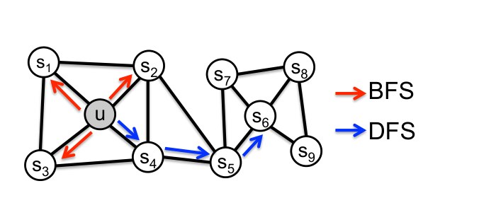
Figure 1: BFS and DFS search strategies from node ().
图 1:从节点 出发的 BFS 和 DFS 搜索策略()。
Recent advancements in representational learning for natural language processing opened new ways for feature learning of discrete objects such as words. In particular, the Skip-gram model [21] aims to learn continuous feature representations for words by optimizing a neighborhood preserving likelihood objective. The algorithm proceeds as follows: It scans over the words of a document, and for every word it aims to embed it such that the word’s features can predict nearby words (i.e., words inside some context window). The word feature representations are learned by optmizing the likelihood objective using SGD with negative sampling [22]. The Skip-gram objective is based on the distributional hypothesis which states that words in similar contexts tend to have similar meanings [9]. That is, similar words tend to appear in similar word neighborhoods.
自然语言处理中表示学习的近期进展,为词这类离散对象的特征学习打开了新途径。尤其是 Skip-gram 模型 [21],通过优化一个保住邻域的似然目标,来学习词的连续特征表示。算法过程如下:它扫描文档中的词,并对每一个词,目标是把它嵌入得使其特征能够预测附近的词(即某个上下文窗口内的词)。词的特征表示通过带负采样的 SGD 优化该似然目标来学习 [22]。Skip-gram 目标基于分布假设,即处于相似上下文中的词往往具有相似的意义 [9]。也就是说,相似的词往往出现在相似的词邻域中。
Inspired by the Skip-gram model, recent research established an analogy for networks by representing a network as a “document” [24, 28]. The same way as a document is an ordered sequence of words, one could sample sequences of nodes from the underlying network and turn a network into a ordered sequence of nodes. However, there are many possible sampling strategies for nodes, resulting in different learned feature representations. In fact, as we shall show, there is no clear winning sampling strategy that works across all networks and all prediction tasks. This is a major shortcoming of prior work which fail to offer any flexibility in sampling of nodes from a network [24, 28]. Our algorithm node2vec overcomes this limitation by designing a flexible objective that is not tied to a particular sampling strategy and provides parameters to tune the explored search space (see Section 3).
受 Skip-gram 模型启发,近期研究通过把网络表示成一篇“文档”,为网络建立了一种类比 [24, 28]。正如文档是词的有序序列,人们可以从底层网络中抽样节点序列,从而把网络变成有序的节点序列。然而,对节点可以有许多种抽样策略,从而得到不同的特征表示。事实上,正如我们将要表明的,并不存在一种在所有网络和所有预测任务上都明显胜出的抽样策略。这是先前工作的一个主要不足:它们未能在从网络中抽样节点时提供任何灵活性 [24, 28]。我们的算法 node2vec 克服了这一限制,它设计了一个并不绑定于特定抽样策略的灵活目标,并提供参数来调节所探索的搜索空间(见第 3 节)。
Finally, for both node and edge based prediction tasks, there is a body of recent work for supervised feature learning based on existing and novel graph-specific deep network architectures [15, 16, 17, 31, 39]. These architectures directly minimize the loss function for a downstream prediction task using several layers of non-linear transformations which results in high accuracy, but at the cost of scalability due to high training time requirements.
最后,对基于节点和基于边的预测任务,近期都有一批基于现有或新颖的图专用深度网络结构的有监督特征学习工作 [15, 16, 17, 31, 39]。这些结构用若干层非线性变换直接最小化下游预测任务的损失函数,精度很高,但由于训练时间需求大,代价是可扩展性不足。
3 Feature learning framework
3 特征学习框架
We formulate feature learning in networks as a maximum likelihood optimization problem. Let be a given network. Our analysis is general and applies to any (un)directed, (un)weighted network. Let be the mapping function from nodes to feature representaions we aim to learn for a downstream prediction task. Here is a parameter specifying the number of dimensions of our feature representation. Equivalently, is a matrix of size parameters. For every source node , we define as a network neighborhood of node generated through a neighborhood sampling strategy .
我们把网络中的特征学习表述为一个极大似然优化问题。设 为给定网络。我们的分析是一般的,适用于任何(无)向、(不)带权的网络。设 是我们希望为下游预测任务学习的、从节点到特征表示的映射函数。这里 是指定特征表示维数的参数。等价地, 是一个大小为 的参数矩阵。对每个源节点 ,我们定义 为通过邻域抽样策略 生成的节点 的网络邻域。
We proceed by extending the Skip-gram architecture to networks [21, 24]. We seek to optimize the following objective function, which maximizes the log-probability of observing a network neighborhood for a node conditioned on its feature representation, given by :
接下来,我们把 Skip-gram 结构扩展到网络 [21, 24]。我们希望优化下面的目标函数,它最大化在给定节点 的特征表示 的条件下,观察到其网络邻域 的对数概率:
In order to make the optimization problem tractable, we make two standard assumptions:
为使优化问题可处理,我们做两个标准假定:
- • Conditional independence. We factorize the likelihood by assuming that the likelihood of observing a neighborhood node is independent of observing any other neighborhood node given the feature representation of the source:
- • 条件独立。我们分解似然,假定在给定源节点特征表示的条件下,观察到某个邻域节点与观察到任何其他邻域节点是独立的:
- • Symmetry in feature space. A source node and neighborhood node have a symmetric effect over each other in feature space. Accordingly, we model the conditional likelihood of every source-neighborhood node pair as a softmax unit parametrized by a dot product of their features:
- • 特征空间中的对称性。源节点和邻域节点在特征空间中彼此具有对称的作用。据此,我们把每一对源节点–邻域节点的条件似然,建模为由它们特征内积参数化的 softmax 单元:
With the above assumptions, the objective in Eq. 1 simplifies to:
在上述假定下,式 1 中的目标简化为:
The per-node partition function, , is expensive to compute for large networks and we approximate it using negative sampling [22]. We optimize Eq. 2 using stochastic gradient ascent over the model parameters defining the features .
每个节点的配分函数 ,对大型网络计算代价很高,我们用负采样来近似它 [22]。我们在定义特征 的模型参数上,用随机梯度上升优化式 2。
Feature learning methods based on the Skip-gram architecture have been originally developed in the context of natural language [21]. Given the linear nature of text, the notion of a neighborhood can be naturally defined using a sliding window over consecutive words. Networks, however, are not linear, and thus a richer notion of a neighborhood is needed. To resolve this issue, we propose a randomized procedure that samples many different neighborhoods of a given source node . The neighborhoods are not restricted to just immediate neighbors but can have vastly different structures depending on the sampling strategy .
基于 Skip-gram 结构的特征学习方法,最初是在自然语言的语境中发展起来的 [21]。鉴于文本的线性性质,邻域的概念可以自然地用在连续词上滑动的窗口来定义。然而网络并不是线性的,因此需要更丰富的邻域概念。为解决这一问题,我们提出一种随机化程序,对给定源节点 抽样许多不同的邻域。邻域 并不局限于直接邻居,而是可以随抽样策略 的不同而具有迥异的结构。
3.1 Classic search strategies
3.1 经典搜索策略
We view the problem of sampling neighborhoods of a source node as a form of local search. Figure 1 shows a graph, where given a source node we aim to generate (sample) its neighborhood . Importantly, to be able to fairly compare different sampling strategies , we shall constrain the size of the neighborhood set to nodes and then sample multiple sets for a single node . Generally, there are two extreme sampling strategies for generating neighborhood set(s) of nodes:
我们把为源节点抽样邻域的问题,视为一种局部搜索。图 1 给出一个图,其中给定源节点 ,我们的目标是生成(抽样)其邻域 。重要的是,为了公平比较不同的抽样策略 ,我们将把邻域集合 的大小约束为 个节点,然后为单个节点 抽样多组这样的集合。一般而言,生成 个节点的邻域集合 ,有两种极端的抽样策略:
- • Breadth-first Sampling (BFS) The neighborhood is restricted to nodes which are immediate neighbors of the source. For example, in Figure 1 for a neighborhood of size , BFS samples nodes , , .
- • 广度优先抽样(BFS) 邻域 被限制为源节点的直接邻居。例如在图 1 中,对大小为 的邻域,BFS 抽到节点 、、。
- • Depth-first Sampling (DFS) The neighborhood consists of nodes sequentially sampled at increasing distances from the source node. In Figure 1, DFS samples , , .
- • 深度优先抽样(DFS) 邻域由与源节点距离递增、依次抽到的节点组成。在图 1 中,DFS 抽到 、、。
The breadth-first and depth-first sampling represent extreme scenarios in terms of the search space they explore leading to interesting implications on the learned representations.
广度优先和深度优先抽样代表了它们所探索搜索空间的两种极端情形,对学到的表示有有意思的含义。
In particular, prediction tasks on nodes in networks often shuttle between two kinds of similarities: homophily and structural equivalence [12]. Under the homophily hypothesis [7, 36] nodes that are highly interconnected and belong to similar network clusters or communities should be embedded closely together (e.g., nodes and in Figure 1 belong to the same network community). In contrast, under the structural equivalence hypothesis [10] nodes that have similar structural roles in networks should be embedded closely together (e.g., nodes and in Figure 1 act as hubs of their corresponding communities). Importantly, unlike homophily, structural equivalence does not emphasize connectivity; nodes could be far apart in the network and still have the same structural role. In real-world, these equivalence notions are not exclusive; networks commonly exhibit both behaviors where some nodes exhibit homophily while others reflect structural equivalence.
尤其是,网络中关于节点的预测任务,常常在两种相似性之间切换:同配性和结构等价 [12]。在同配性假设下 [7, 36],高度相互连接、同属相似网络簇或社区的节点,应当被嵌入得靠近(例如,图 1 中的节点 和 同属一个网络社区)。相对地,在结构等价假设下 [10],在网络中具有相似结构角色的节点应当被嵌入得靠近(例如,图 1 中的节点 和 充当各自社区的枢纽)。重要的是,与同配性不同,结构等价并不强调连通性;节点在网络中可以相距很远,却仍有相同的结构角色。在现实世界中,这些等价概念并非互斥;网络通常会同时表现出两种行为,一些节点体现同配性,另一些则反映结构等价。
We observe that BFS and DFS strategies play a key role in producing representations that reflect either of the above equivalences. In particular, the neighborhoods sampled by BFS lead to embeddings that correspond closely to structural equivalence. Intuitively, we note that in order to ascertain structural equivalence, it is often sufficient to characterize the local neighborhoods accurately. For example, structural equivalence based on network roles such as bridges and hubs can be inferred just by observing the immediate neighborhoods of each node. By restricting search to nearby nodes, BFS achieves this characterization and obtains a microscopic view of the neighborhood of every node. Additionally, in BFS, nodes in the sampled neighborhoods tend to repeat many times. This is also important as it reduces the variance in characterizing the distribution of 1-hop nodes with respect the source node. However, a very small portion of the graph is explored for any given .
我们观察到,BFS 和 DFS 策略在产生反映上述某一种等价性的表示时起着关键作用。具体而言,由 BFS 抽到的邻域会导向与结构等价密切相关的嵌入。直观上,要确定结构等价,往往只需准确地刻画局部邻域就足够了。例如,基于桥和枢纽这类网络角色的结构等价,只需观察每个节点的直接邻域就能推断。通过把搜索限制在附近节点,BFS 实现了这种刻画,并得到每个节点邻域的微观视图。此外,在 BFS 中,抽到的邻域里的节点往往会多次重复。这一点也很重要,因为它降低了刻画相对源节点的 1 跳节点分布时的方差。不过,对任意给定的 ,所探索的图的部分都非常小。
The opposite is true for DFS which can explore larger parts of the network as it can move further away from the source node (with sample size being fixed). In DFS, the sampled nodes more accurately reflect a macro-view of the neighborhood which is essential in inferring communities based on homophily. However, the issue with DFS is that it is important to not only infer which node-to-node dependencies exist in a network, but also to characterize the exact nature of these dependencies. This is hard given we have a constrain on the sample size and a large neighborhood to explore, resulting in high variance. Secondly, moving to much greater depths leads to complex dependencies since a sampled node may be far from the source and potentially less representative.
DFS 则正好相反:在样本量 固定时,它能离源节点 更远,从而探索网络中更大的部分。在 DFS 中,抽到的节点更能反映邻域的宏观视图,而这对基于同配性推断社区是必要的。不过,DFS 的问题在于,重要的不仅是推断网络中存在哪些节点到节点的依赖,还要刻画这些依赖的确切性质。鉴于样本量有约束、而要探索的邻域又很大,这很困难,从而带来高方差。其次,走到深得多的地方会导致复杂的依赖,因为抽到的节点可能离源节点很远,代表性也潜在地更弱。
3.2 node2vec
Building on the above observations, we design a flexible neighborhood sampling strategy which allows us to smoothly interpolate between BFS and DFS. We achieve this by developing a flexible biased random walk procedure that can explore neighborhoods in a BFS as well as DFS fashion.
基于上述观察,我们设计一种灵活的邻域抽样策略,使我们能在 BFS 和 DFS 之间平滑插值。我们通过发展一种灵活的带偏置随机游走过程来做到这一点,它既能以 BFS 方式、也能以 DFS 方式探索邻域。
3.2.1 Random Walks
Formally, given a source node , we simulate a random walk of fixed length . Let denote the th node in the walk, starting with . Nodes are generated by the following distribution:
3.2.1 随机游走
形式地,给定源节点 ,我们模拟一条长度为固定值 的随机游走。记 为游走中的第 个节点,起点为 。节点 由下面的分布生成:
$$P(c_{i}=x\mid c_{i-1}=v)=\begin{cases}\frac{\pi_{vx}}{Z}&\text{if }(v,x)\in E\
0&\text{otherwise}\end{cases}$$
where is the unnormalized transition probability between nodes and , and is the normalizing constant.
其中 是节点 与 之间未经归一化的转移概率, 是归一化常数。
3.2.2 Search bias
The simplest way to bias our random walks would be to sample the next node based on the static edge weights i.e., . (In case of unweighted graphs .) However, this does not allow us to account for the network structure and guide our search procedure to explore different types of network neighborhoods. Additionally, unlike BFS and DFS which are extreme sampling paradigms suited for structural equivalence and homophily respectively, our random walks should accommodate for the fact that these notions of equivalence are not competing or exclusive, and real-world networks commonly exhibit a mixture of both.
3.2.2 搜索偏置
给我们的随机游走加偏置,最简单的方式是按静态边权 抽样下一个节点,即 。(对不带权图,。)不过,这并不能让我们把网络结构考虑进来,并引导搜索程序去探索不同类型的网络邻域。此外,与分别适合结构等价和同配性的极端抽样范式 BFS 和 DFS 不同,我们的随机游走应当顾及到:这些等价概念并非相互竞争或互斥,真实网络通常会同时表现出二者的混合。
We define a 2 order random walk with two parameters and which guide the walk: Consider a random walk that just traversed edge and now resides at node (Figure 2). The walk now needs to decide on the next step so it evaluates the transition probabilities on edges leading from . We set the unnormalized transition probability to , where
我们定义一种带两个参数 和 的二阶随机游走,由它们来引导游走:考虑一条刚走过边 、现在位于节点 的随机游走(图 2)。游走现在需要决定下一步,因此它评估从 出发的各边 上的转移概率 。我们把未经归一化的转移概率设为 ,其中
$$\alpha_{pq}(t,x)=\begin{cases}\frac{1}{p}&\text{if }d_{tx}=0\
1&\text{if }d_{tx}=1\
\frac{1}{q}&\text{if }d_{tx}=2\end{cases}$$
and denotes the shortest path distance between nodes and . Note that must be one of , and hence, the two parameters are necessary and sufficient to guide the walk.
而 表示节点 与 之间的最短路径距离。注意 必须是 之一,因此这两个参数对于引导游走是必要且充分的。
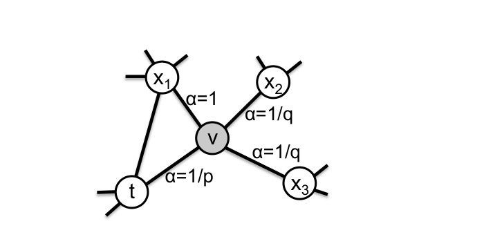
Figure 2: Illustration of the random walk procedure in node2vec. The walk just transitioned from to and is now evaluating its next step out of node . Edge labels indicate search biases .
图 2:node2vec 中随机游走过程的示意。游走刚从 转移到 ,现在正在评估从节点 出发的下一步。边上的标记表示搜索偏置 。
Intuitively, parameters and control how fast the walk explores and leaves the neighborhood of starting node . In particular, the parameters allow our search procedure to (approximately) interpolate between BFS and DFS and thereby reflect an affinity for different notions of node equivalences.
直观上,参数 和 控制游走探索并离开起始节点 邻域的快慢。具体而言,这些参数使我们的搜索程序能够(近似地)在 BFS 和 DFS 之间插值,从而反映出对不同节点等价概念的偏好。
Return parameter, . Parameter controls the likelihood of immediately revisiting a node in the walk. Setting it to a high value () ensures that we are less likely to sample an already-visited node in the following two steps (unless the next node in the walk had no other neighbor). This strategy encourages moderate exploration and avoids -hop redundancy in sampling. On the other hand, if is low (), it would lead the walk to backtrack a step (Figure 2) and this would keep the walk “local” close to the starting node .
返回参数 。 参数 控制在游走中立即重访一个节点的可能性。把它设成较大的值(),可以确保在接下来的两步里不太可能抽到已经访问过的节点(除非游走中的下一节点没有别的邻居)。这种策略鼓励适度探索,并避免抽样中的 2 跳冗余。另一方面,若 较小(),则会引导游走回溯一步(图 2),从而使游走保持“局部”,靠近起始节点 。
In-out parameter, . Parameter allows the search to differentiate between “inward” and “outward” nodes. Going back to Figure 2, if , the random walk is biased towards nodes close to node . Such walks obtain a local view of the underlying graph with respect to the start node in the walk and approximate BFS behavior in the sense that our samples comprise of nodes within a small locality.
进出参数 。 参数 使搜索能够区分“向内”和“向外”的节点。回到图 2,若 ,随机游走会偏向靠近节点 的节点。这样的游走相对于游走的起始节点,得到底层图的局部视图,并近似 BFS 的行为,因为我们的样本由一个小局部内的节点组成。
In contrast, if , the walk is more inclined to visit nodes which are further away from the node . Such behavior is reflective of DFS which encourages outward exploration. However, an essential difference here is that we achieve DFS-like exploration within the random walk framework. Hence, the sampled nodes are not at strictly increasing distances from a given source node , but in turn, we benefit from tractable preprocessing and superior sampling efficiency of random walks. Note that by setting to be a function of the preceeding node in the walk , the random walks are 2 order Markovian.
相对地,若 ,游走更倾向于访问离节点 更远的节点。这种行为反映了鼓励向外探索的 DFS。不过,这里一个关键差别是,我们是在随机游走的框架内实现类似 DFS 的探索。因此,抽到的节点并非与给定源节点 的距离严格递增,但作为回报,我们受益于随机游走可处理的预处理和更优的抽样效率。注意,通过把 设为游走中前一节点 的函数,这些随机游走是二阶马尔可夫的。
Benefits of random walks. There are several benefits of random walks over pure BFS/DFS approaches. Random walks are computationally efficient in terms of both space and time requirements. The space complexity to store the immediate neighbors of every node in the graph is . For 2 order random walks, it is helpful to store the interconnections between the neighbors of every node, which incurs a space complexity of where is the average degree of the graph and is usually small for real-world networks. The other key advantage of random walks over classic search-based sampling strategies is its time complexity. In particular, by imposing graph connectivity in the sample generation process, random walks provide a convenient mechanism to increase the effective sampling rate by reusing samples across different source nodes. By simulating a random walk of length we can generate samples for nodes at once due to the Markovian nature of the random walk. Hence, our effective complexity is per sample. For example, in Figure 1 we sample a random walk of length , which results in , and . Note that sample reuse can introduce some bias in the overall procedure. However, we observe that it greatly improves the efficiency.
随机游走的好处。 相对纯粹的 BFS/DFS 方法,随机游走有若干好处。随机游走在空间和时间需求上都计算高效。存储图中每个节点的直接邻居的空间复杂度是 。对二阶随机游走,存储每个节点的邻居之间的相互连接是有帮助的,这会带来 的空间复杂度,其中 是图的平均度,对真实网络通常较小。随机游走相对经典的基于搜索的抽样策略的另一关键优势是时间复杂度。具体而言,通过在样本生成过程中施加图的连通性,随机游走提供了一种便捷机制,通过在不同源节点之间复用样本来提高有效抽样率。通过模拟一条长度为 的随机游走,由于随机游走的马尔可夫性质,我们可以一次为 个节点各生成 个样本。因此,每个样本的有效复杂度是 。例如在图 1 中,我们抽一条长度为 的随机游走 ,从而得到 , 以及 。需要注意,样本复用会在整个程序中引入一些偏差。不过,我们观察到它极大地提高了效率。
3.2.3 The node2vec algorithm
LearnFeatures (Graph , Dimensions , Walks per node , Walk length , Context size , Return , In-out )
PreprocessModifiedWeights()
Initialize to Empty
for to do
for all nodes do
node2vecWalk()
Append to
StochasticGradientDescent(, , )
return
node2vecWalk (Graph , Start node , Length )
Inititalize to
for to do
GetNeighbors(, )
AliasSample()
Append to
return
Algorithm 1 The node2vec algorithm.
3.2.3 node2vec 算法
LearnFeatures(图 ,维数 ,每节点游走数 ,游走长度 ,上下文大小 ,返回 ,进出 )
PreprocessModifiedWeights()
将 初始化为空
for to do
for all 节点 do
node2vecWalk()
把 追加到
StochasticGradientDescent(, , )
return
node2vecWalk(图 ,起始节点 ,长度 )
将 初始化为
for to do
GetNeighbors(, )
AliasSample()
把 追加到
return
算法 1 node2vec 算法。
The pseudocode for node2vec, is given in Algorithm 1. In any random walk, there is an implicit bias due to the choice of the start node . Since we learn representations for all nodes, we offset this bias by simulating random walks of fixed length starting from every node. At every step of the walk, sampling is done based on the transition probabilities . The transition probabilities for the 2 order Markov chain can be precomputed and hence, sampling of nodes while simulating the random walk can be done efficiently in time using alias sampling. The three phases of node2vec, i.e., preprocessing to compute transition probabilities, random walk simulations and optimization using SGD, are executed sequentially. Each phase is parallelizable and executed asynchronously, contributing to the overall scalability of node2vec.
node2vec 的伪代码见算法 1。在任何随机游走中,由于起始节点 的选择,都会有一种隐含的偏差。由于我们要为所有节点学习表示,我们通过从每一个节点出发,模拟 条长度为固定值 的随机游走,来抵消这一偏差。在游走的每一步,抽样依据转移概率 进行。二阶马尔可夫链的转移概率 可以预先计算,因此在模拟随机游走时,可以用 alias sampling 以 时间高效地抽节点。node2vec 的三个阶段,即计算转移概率的预处理、随机游走模拟,以及用 SGD 做优化,是顺序执行的。每个阶段都可以并行化并以异步方式执行,这有助于 node2vec 的整体可扩展性。
node2vec is available at: http://snap.stanford.edu/node2vec.
node2vec 可在以下地址获得:http://snap.stanford.edu/node2vec。
| Operator | Symbol | Definition |
|---|---|---|
| Average | ||
| Hadamard | ||
| Weighted-L1 | $\ | \cdot\ |
| Weighted-L2 | $\ | \cdot\ |
Table 1: Choice of binary operators for learning edge features. The definitions correspond to the th component of .
| 算子 | 符号 | 定义 |
|---|---|---|
| 平均 | ||
| Hadamard | ||
| 加权 | ||
| 加权 |
表 1:学习边特征时二元算子 的选择。定义对应于 的第 个分量。
3.3 Learning edge features
3.3 学习边特征
The node2vec algorithm provides a semi-supervised method to learn rich feature representations for nodes in a network. However, we are often interested in prediction tasks involving pairs of nodes instead of individual nodes. For instance, in link prediction, we predict whether a link exists between two nodes in a network. Since our random walks are naturally based on the connectivity structure between nodes in the underlying network, we extend them to pairs of nodes using a bootstrapping approach over the feature representations of the individual nodes.
node2vec 算法提供了一种半监督方法,为网络中的节点学习丰富的特征表示。不过,我们常常对涉及节点对而非单个节点的预测任务感兴趣。例如在链接预测中,我们预测网络中两个节点之间是否存在一条链接。由于我们的随机游走自然基于底层网络中节点之间的连通结构,我们用一种在各个节点特征表示上的自助(bootstrapping)方法,把它们扩展到节点对。
Given two nodes and , we define a binary operator over the corresponding feature vectors and in order to generate a representation such that where is the representation size for the pair . We want our operators to be generally defined for any pair of nodes, even if an edge does not exist between the pair since doing so makes the representations useful for link prediction where our test set contains both true and false edges (i.e., do not exist). We consider several choices for the operator such that which are summarized in Table 1.
给定两个节点 和 ,我们在相应的特征向量 和 上定义一个二元算子 ,以生成表示 ,使得 ,其中 是配对 的表示大小。我们希望算子对任意节点对都一般地有定义,即使这对节点之间并不存在边,因为这样做会使表示对链接预测有用——测试集中既包含真实边,也包含不存在的假边。我们考虑若干使 的算子 选择,总结于表 1。
4 Experiments
4 实验
The objective in Eq. 2 is independent of any downstream task and the flexibility in exploration offered by node2vec lends the learned feature representations to a wide variety of network analysis settings discussed below.
式 2 中的目标与任何下游任务无关,而 node2vec 在探索上提供的灵活性,使学到的特征表示可以用于下面讨论的多种网络分析设定。
4.1 Case Study: Les Misérables network
4.1 案例研究:《悲惨世界》网络
In Section 3.1 we observed that BFS and DFS strategies represent extreme ends on the spectrum of embedding nodes based on the principles of homophily (i.e., network communities) and structural equivalence (i.e., structural roles of nodes). We now aim to empirically demonstrate this fact and show that node2vec in fact can discover embeddings that obey both principles.
在第 3.1 节中我们观察到,BFS 和 DFS 策略代表了按同配性(即网络社区)和结构等价(即节点的结构角色)嵌入节点这一谱系的两个极端。我们现在希望经验地证明这一点,并表明 node2vec 事实上可以发现同时服从这两条原则的嵌入。
We use a network where nodes correspond to characters in the novel Les Misérables [13] and edges connect coappearing characters. The network has 77 nodes and 254 edges. We set and run node2vec to learn feature representation for every node in the network. The feature representations are clustered using -means. We then visualize the original network in two dimensions with nodes now assigned colors based on their clusters.
我们使用一个网络,其中节点对应于小说《悲惨世界》中的人物 [13],边连接共同出现的人物。该网络有 77 个节点和 254 条边。我们设 并运行 node2vec,为网络中的每个节点学习特征表示。特征表示用 -means 聚类。然后我们在二维中可视化原始网络,节点的颜色按其所属簇来指定。
Figure 3(top) shows the example when we set . Notice how regions of the network (i.e., network communities) are colored using the same color. In this setting node2vec discovers clusters/communities of characters that frequently interact with each other in the major sub-plots of the novel. Since the edges between characters are based on coappearances, we can conclude this characterization closely relates with homophily.
图 3(上)给出了设 时的例子。注意网络的各个区域(即网络社区)是如何用同一种颜色着色的。在这一设置下,node2vec 发现了在小说主要情节中频繁互动的人物簇 / 社区。由于人物之间的边基于共同出现,我们可以断定这种刻画与同配性密切相关。
In order to discover which nodes have the same structural roles we use the same network but set , use node2vec to get node features and then cluster the nodes based on the obtained features. Here node2vec obtains a complementary assignment of node to clusters such that the colors correspond to structural equivalence as illustrated in Figure 3(bottom). For instance, node2vec embeds blue-colored nodes close together. These nodes represent characters that act as bridges between different sub-plots of the novel. Similarly, the yellow nodes mostly represent characters that are at the periphery and have limited interactions. One could assign alternate semantic interpretations to these clusters of nodes, but the key takeaway is that node2vec is not tied to a particular notion of equivalence. As we show through our experiments, these equivalence notions are commonly exhibited in most real-world networks and have a significant impact on the performance of the learned representations for prediction tasks.
为了发现哪些节点具有相同的结构角色,我们使用同一个网络,但设 ,用 node2vec 得到节点特征,再基于所得特征对节点聚类。此时 node2vec 得到一种互补的节点到簇的分配,使得颜色对应于结构等价,如图 3(下)所示。例如,node2vec 把蓝色节点嵌入得靠近。这些节点代表在小说不同情节之间充当桥梁的人物。类似地,黄色节点大多代表处于边缘、互动有限的人物。人们也可以给这些节点簇赋予别的语义解释,但关键收获是:node2vec 并不绑定于某一种特定的等价概念。正如我们将通过实验表明的,这些等价概念在大多数真实网络中普遍存在,并对学到的表示在预测任务上的表现有显著影响。
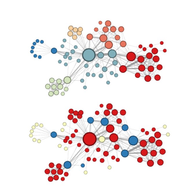
Figure 3: Complementary visualizations of Les Misérables coappearance network generated by node2vec with label colors reflecting homophily (top) and structural equivalence (bottom).
图 3:由 node2vec 生成的《悲惨世界》共现网络的互补可视化,标签颜色分别反映同配性(上)和结构等价(下)。
4.2 Experimental setup
4.2 实验设置
Our experiments evaluate the feature representations obtained through node2vec on standard supervised learning tasks: multi-label classification for nodes and link prediction for edges. For both tasks, we evaluate the performance of node2vec against the following feature learning algorithms:
我们的实验在标准的监督学习任务上评估通过 node2vec 得到的特征表示:针对节点的多标签分类,以及针对边的链接预测。对这两项任务,我们把 node2vec 的表现与下列特征学习算法相对照:
- • Spectral clustering [29]: This is a matrix factorization approach in which we take the top eigenvectors of the normalized Laplacian matrix of graph as the feature vector representations for nodes.
- • 谱聚类 [29]:这是一种矩阵分解方法,我们取图 的归一化拉普拉斯矩阵的前 个特征向量,作为节点的特征向量表示。
- • DeepWalk [24]: This approach learns -dimensional feature representations by simulating uniform random walks. The sampling strategy in DeepWalk can be seen as a special case of node2vec with and .
- • DeepWalk [24]:该方法通过模拟均匀随机游走来学习 维特征表示。DeepWalk 中的抽样策略可以视为 且 时 node2vec 的一个特例。
- • LINE [28]: This approach learns -dimensional feature representations in two separate phases. In the first phase, it learns dimensions by BFS-style simulations over immediate neighbors of nodes. In the second phase, it learns the next dimensions by sampling nodes strictly at a 2-hop distance from the source nodes.
- • LINE [28]:该方法分两个独立阶段学习 维特征表示。第一阶段,它通过对节点的直接邻居做 BFS 式模拟,学习 维。第二阶段,它通过严格在源节点的 2 跳距离上抽样节点,学习接下来的 维。
We exclude other matrix factorization approaches which have already been shown to be inferior to DeepWalk [24]. We also exclude a recent approach, GraRep [6], that generalizes LINE to incorporate information from network neighborhoods beyond 2-hops, but is unable to efficiently scale to large networks.
我们排除了其他已被证明不如 DeepWalk 的矩阵分解方法 [24]。我们也排除了近期的 GraRep [6],它把 LINE 推广到纳入超过 2 跳的网络邻域信息,但无法高效地扩展到大型网络。
In contrast to the setup used in prior work for evaluating sampling-based feature learning algorithms, we generate an equal number of samples for each method and then evaluate the quality of the obtained features on the prediction task. In doing so, we discount for performance gain observed purely because of the implementation language (C/C++/Python) since it is secondary to the algorithm. Thus, in the sampling phase, the parameters for DeepWalk, LINE and node2vec are set such that they generate equal number of samples at runtime. As an example, if is the overall sampling budget, then the node2vec parameters satisfy . In the optimization phase, all these benchmarks optimize using SGD with two key differences that we correct for. First, DeepWalk uses hierarchical sampling to approximate the softmax probabilities with an objective similar to the one use by node2vec. However, hierarchical softmax is inefficient when compared with negative sampling [22]. Hence, keeping everything else the same, we switch to negative sampling in DeepWalk which is also the de facto approximation in node2vec and LINE. Second, both node2vec and DeepWalk have a parameter for the number of context neighborhood nodes to optimize for and the greater the number, the more rounds of optimization are required. This parameter is set to unity for LINE, but since LINE completes a single epoch quicker than other approaches, we let it run for epochs.
与先前工作评估基于抽样的特征学习算法时所采用的设置不同,我们为每种方法生成同等数量的样本,再在预测任务上评估所得特征的质量。这样做,是为了剔除仅仅因为实现语言(C/C++/Python)而观察到的性能增益,因为这对算法本身是次要的。因此,在抽样阶段,DeepWalk、LINE 和 node2vec 的参数被设置成在运行时生成同等数量的样本。作为例子,若 是总的抽样预算,则 node2vec 的参数满足 。在优化阶段,所有这些对照方法都用 SGD 优化,但有两处关键差别我们做了校正。第一,DeepWalk 用层次化抽样来近似 softmax 概率,其目标与 node2vec 所用的类似。不过,与负采样相比,层次 softmax 效率较低 [22]。因此,在其他一切不变的前提下,我们把 DeepWalk 改成负采样,这也是 node2vec 和 LINE 中实际上采用的近似。第二,node2vec 和 DeepWalk 都有一个要为之优化的上下文邻域节点数目参数,该数目越大,所需的优化轮次就越多。这一参数对 LINE 被设为 1,但由于 LINE 完成单个轮次比其他方法更快,我们让它运行 个轮次。
The parameter settings used for node2vec are in line with typical values used for DeepWalk and LINE. Specifically, we set , , , , and the optimization is run for a single epoch. We repeat our experiments for random seed initializations, and our results are statistically significant with a p-value of less than 0.01.The best in-out and return hyperparameters were learned using 10-fold cross-validation on 10% labeled data with a grid search over .
node2vec 所用的参数设置与 DeepWalk 和 LINE 的典型取值一致。具体地,我们设 ,,,,优化运行单个轮次。我们用 次随机种子初始化重复实验,结果在 p 值小于 0.01 的意义下具有统计显著性。最好的进出和返回超参数,是在 10% 带标签数据上用 10 折交叉验证、并在 上做网格搜索学到的。
4.3 Multi-label classification
4.3 多标签分类
| Algorithm | Dataset | ||
|---|---|---|---|
| BlogCatalog | PPI | Wikipedia | |
| Spectral Clustering | 0.0405 | 0.0681 | 0.0395 |
| DeepWalk | 0.2110 | 0.1768 | 0.1274 |
| LINE | 0.0784 | 0.1447 | 0.1164 |
| node2vec | 0.2581 | 0.1791 | 0.1552 |
| node2vec settings (p,q) | 0.25, 0.25 | 4, 1 | 4, 0.5 |
| Gain ofnode2vec**[%]** | 22.3 | 1.3 | 21.8 |
Table 2: Macro-F1 scores for multilabel classification on BlogCatalog, PPI (Homo sapiens) and Wikipedia word cooccurrence networks with 50% of the nodes labeled for training.
| 算法 | 数据集 | ||
|---|---|---|---|
| BlogCatalog | PPI | Wikipedia | |
| 谱聚类 | 0.0405 | 0.0681 | 0.0395 |
| DeepWalk | 0.2110 | 0.1768 | 0.1274 |
| LINE | 0.0784 | 0.1447 | 0.1164 |
| node2vec | 0.2581 | 0.1791 | 0.1552 |
| node2vec 设置 (p,q) | 0.25, 0.25 | 4, 1 | 4, 0.5 |
| node2vec 的增益 [%] | 22.3 | 1.3 | 21.8 |
表 2:在 BlogCatalog、PPI(智人)和维基词共现网络上,用 50% 节点作为训练标签时的多标签分类 Macro-F1 分数。
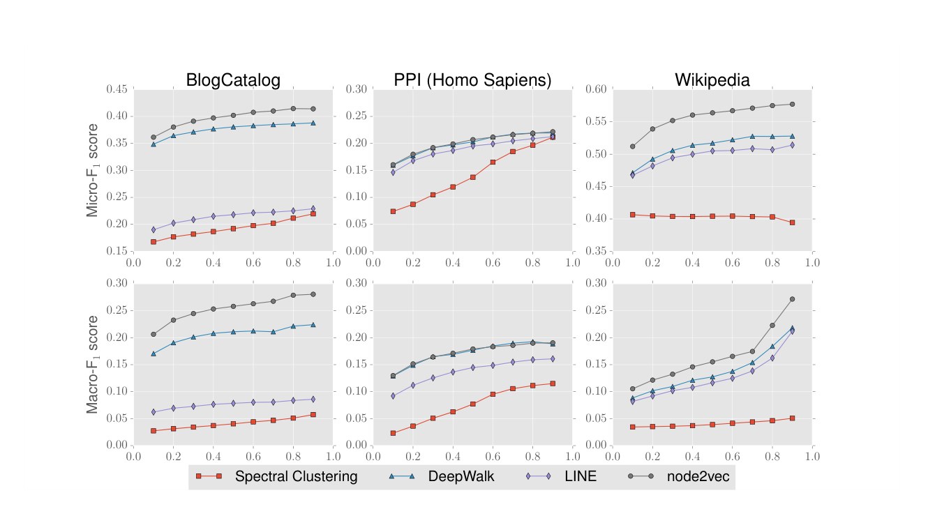
Figure 4: Performance evaluation of different benchmarks on varying the amount of labeled data used for training. The axis denotes the fraction of labeled data, whereas the axis in the top and bottom rows denote the Micro-F1 and Macro-F1 scores respectively. DeepWalk and node2vec give comparable performance on PPI. In all other networks, across all fractions of labeled data node2vec performs best.
图 4:在改变用于训练的带标签数据量时,不同对照方法的性能评估。 轴表示带标签数据的比例,上、下两行的 轴分别表示 Micro-F1 和 Macro-F1 分数。DeepWalk 和 node2vec 在 PPI 上表现相当。在所有其他网络上,对所有带标签数据比例,都是 node2vec 表现最好。
In the multi-label classification setting, every node is assigned one or more labels from a finite set . During the training phase, we observe a certain fraction of nodes and all their labels. The task is to predict the labels for the remaining nodes. This is a challenging task especially if is large. We utilize the following datasets:
在多标签分类设定中,每个节点被赋予有限集合 中的一个或多个标签。在训练阶段,我们观察到一定比例的节点及其全部标签。任务是为其余节点预测标签。若 很大,这是一项有挑战的任务。我们使用下列数据集:
- • BlogCatalog [38]: This is a network of social relationships of the bloggers listed on the BlogCatalog website. The labels represent blogger interests inferred through the meta-data provided by the bloggers. The network has 10,312 nodes, 333,983 edges, and 39 different labels.
- • BlogCatalog [38]:这是 BlogCatalog 网站上所列博客作者社交关系的网络。标签表示通过博主提供的元数据推断出的兴趣。该网络有 10,312 个节点、333,983 条边和 39 种不同标签。
- • Protein-Protein Interactions (PPI) [5]: We use a subgraph of the PPI network for Homo Sapiens. The subgraph corresponds to the graph induced by nodes for which we could obtain labels from the hallmark gene sets [19] and represent biological states. The network has 3,890 nodes, 76,584 edges, and 50 different labels.
- • 蛋白质相互作用(PPI) [5]:我们使用智人 PPI 网络的一个子图。该子图由我们能够从标志性基因集 [19] 获得标签、并表示生物学状态的节点所诱导。该网络有 3,890 个节点、76,584 条边和 50 种不同标签。
- • Wikipedia [20]: This is a cooccurrence network of words appearing in the first million bytes of the Wikipedia dump. The labels represent the Part-of-Speech (POS) tags inferred using the Stanford POS-Tagger [32]. The network has 4,777 nodes, 184,812 edges, and 40 different labels.
- • Wikipedia [20]:这是出现在维基百科转储前一百万字节中的词的共现网络。标签表示用斯坦福词性标注器 [32] 推断出的词性(POS)标记。该网络有 4,777 个节点、184,812 条边和 40 种不同标签。
All these networks exhibit a fair mix of homophilic and structural equivalences. For example, we expect the social network of bloggers to exhibit strong homophily-based relationships; however, there might also be some “familiar strangers”, i.e., bloggers that do not interact but share interests and hence are structurally equivalent nodes. The biological states of proteins in a protein-protein interaction network also exhibit both types of equivalences. For example, they exhibit structural equivalence when proteins perform functions complementary to those of neighboring proteins, and at other times, they organize based on homophily in assisting neighboring proteins in performing similar functions. The word cooccurence network is fairly dense, since edges exist between words cooccuring in a 2-length window in the Wikipedia corpus. Hence, words having the same POS tags are not hard to find, lending a high degree of homophily. At the same time, we expect some structural equivalence in the POS tags due to syntactic grammar patterns such as nouns following determiners, punctuations succeeding nouns etc.
这些网络都表现出同配性与结构等价的相当混合。例如,我们预期博主的社交网络会表现出很强的基于同配性的关系;不过,也可能存在一些“熟悉的陌生人”,即并不互动却分享兴趣、因而在结构上等价的博主。蛋白质相互作用网络中蛋白质的生物学状态也同时表现出两类等价。例如,当蛋白质履行与邻近蛋白质互补的功能时,它们表现出结构等价;在另一些时候,它们又按同配性组织起来,协助邻近蛋白质履行相似的功能。词共现网络相当稠密,因为维基语料中在长度为 2 的窗口内共现的词之间都有边。因此,具有相同词性标记的词并不难找到,带来了高度的同配性。与此同时,由于句法模式,例如名词跟在限定词之后、标点跟在名词之后等,我们也预期词性标记中会有一些结构等价。
Experimental results. The node feature representations are input to a one-vs-rest logistic regression classifier with L2 regularization. The train and test data is split equally over 10 random instances. We use the Macro-F1 scores for comparing performance in Table 2 and the relative performance gain is over the closest benchmark. The trends are similar for Micro-F1 and accuracy and are not shown.
实验结果。 节点特征表示被输入到带 L2 正则的一对多逻辑回归分类器。训练和测试数据在 10 次随机划分中各占一半。我们用 Macro-F1 分数在表 2 中比较性能,相对增益是相对最接近的对照方法而言的。Micro-F1 和准确率的趋势类似,不再给出。
From the results, it is evident we can see how the added flexibility in exploring neighborhoods allows node2vec to outperform the other benchmark algorithms. In BlogCatalog, we can discover the right mix of homophily and structural equivalence by setting parameters and to low values, giving us 22.3% gain over DeepWalk and 229.2% gain over LINE in Macro-F1 scores. LINE showed worse performance than expected, which can be explained by its inability to reuse samples, a feat that can be easily done using the random walk methods. Even in our other two networks, where we have a mix of equivalences present, the semi-supervised nature of node2vec can help us infer the appropriate degree of exploration necessary for feature learning. In the case of PPI network, the best exploration strategy (, ) turns out to be virtually indistinguishable from DeepWalk’s uniform (, ) exploration giving us only a slight edge over DeepWalk by avoiding redudancy in already visited nodes through a high value, but a convincing 23.8% gain over LINE in Macro-F1 scores. However, in general, the uniform random walks can be much worse than the exploration strategy learned by node2vec. As we can see in the Wikipedia word cooccurrence network, uniform walks cannot guide the search procedure towards the best samples and hence, we achieve a gain of 21.8% over DeepWalk and 33.2% over LINE.
从结果可以明显看出,探索邻域时增加的灵活性如何使 node2vec 超过其他对照算法。在 BlogCatalog 中,通过把参数 和 设成较小的值,我们可以发现同配性与结构等价的合适混合,从而在 Macro-F1 分数上相对 DeepWalk 获得 22.3% 的增益,相对 LINE 获得 229.2% 的增益。LINE 的表现比预期更差,这可以由它无法复用样本来解释,而随机游走方法很容易做到这一点。即使在我们另外两个存在等价性混合的网络中,node2vec 的半监督性质也能帮助我们推断特征学习所需的合适探索程度。在 PPI 网络上,最好的探索策略(,)实际上与 DeepWalk 的均匀探索(,)几乎无法区分,只通过较大的 值避免了已访问节点上的冗余,从而相对 DeepWalk 只有轻微优势,但在 Macro-F1 分数上相对 LINE 仍有令人信服的 23.8% 增益。不过一般而言,均匀随机游走可能比 node2vec 学到的探索策略差得多。正如我们在维基词共现网络中看到的,均匀游走无法把搜索程序引向最好的样本,因此我们相对 DeepWalk 获得 21.8% 的增益,相对 LINE 获得 33.2% 的增益。
For a more fine-grained analysis, we also compare performance while varying the train-test split from 10% to 90%, while learning parameters and on 10% of the data as before. For brevity, we summarize the results for the Micro-F1 and Macro-F1 scores graphically in Figure 4. Here we make similar observations. All methods significantly outperform Spectral clustering, DeepWalk outperforms LINE, node2vec consistently outperforms LINE and achieves large improvement over DeepWalk across domains. For example, we achieve the biggest improvement over DeepWalk of 26.7% on BlogCatalog at 70% labeled data. In the worst case, the search phase has little bearing on learned representations in which case node2vec is equivalent to DeepWalk. Similarly, the improvements are even more striking when compared to LINE, where in addition to drastic gain (over 200%) on BlogCatalog, we observe high magnitude improvements upto 41.1% on other datasets such as PPI while training on just 10% labeled data.
为了做更细粒度的分析,我们还在把训练–测试划分从 10% 变到 90% 的同时比较性能,并像之前一样在 10% 的数据上学习参数 和 。为简明起见,我们把 Micro-F1 和 Macro-F1 分数的结果用图 4 加以概括。这里我们做出类似的观察。所有方法都显著超过谱聚类,DeepWalk 超过 LINE,node2vec 则一贯超过 LINE,并在不同领域上相对 DeepWalk 取得大幅度改进。例如,我们在 BlogCatalog、70% 带标签数据时,相对 DeepWalk 取得了最大的 26.7% 改进。在最差的情形下,搜索阶段对学到的表示影响很小,此时 node2vec 等价于 DeepWalk。类似地,与 LINE 相比,改进甚至更为显著:除了在 BlogCatalog 上超过 200% 的大幅度增益外,我们还在其他数据集如 PPI 上,仅用 10% 带标签数据训练时,观察到高达 41.1% 的改进。
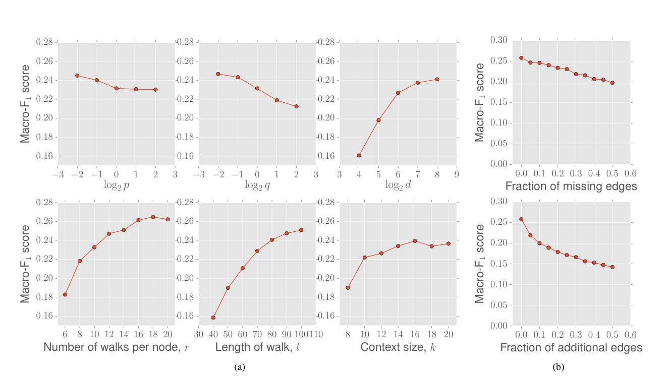
Figure 5: (a). Parameter sensitivity (b). Perturbation analysis for multilabel classification on the BlogCatalog network.
图 5:(a)参数敏感性;(b)在 BlogCatalog 网络上多标签分类的扰动分析。
4.4 Parameter sensitivity
4.4 参数敏感性
The node2vec algorithm involves a number of parameters and in Figure 5(a), we examine how the different choices of parameters affect the performance of node2vec on the BlogCatalog dataset using a 50-50 split between labeled and unlabeled data. Except for the parameter being tested, all other parameters assume default values. The default values for and are set to unity.
node2vec 算法涉及若干参数。在图 5(a) 中,我们考察不同参数选择如何影响 node2vec 在 BlogCatalog 数据集上的表现,带标签与未标注数据按 50-50 划分。除正在测试的参数外,其余参数都取默认值。 和 的默认值设为 1。
We measure the Macro-F1 score as a function of parameters and . The performance of node2vec improves as the in-out parameter and the return parameter decrease. This increase in performance can be based on the homophilic and structural equivalences we expect to see in BlogCatalog. While a low encourages outward exploration, it is balanced by a low which ensures that the walk does not go too far from the start node.
我们把 Macro-F1 分数作为参数 和 的函数来度量。随着进出参数 和返回参数 减小,node2vec 的性能会提高。这一提升可以基于我们预期在 BlogCatalog 中看到的同配性和结构等价来解释。较小的 鼓励向外探索,同时又被较小的 所平衡,后者确保游走不会离起始节点太远。
We also examine how the number of features and the node’s neighborhood parameters (number of walks , walk length , and neighborhood size ) affect the performance. We observe that performance tends to saturate once the dimensions of the representations reaches around 100. Similarly, we observe that increasing the number and length of walks per source improves performance, which is not surprising since we have a greater overall sampling budget to learn representations. Both these parameters have a relatively high impact on the performance of the method. Interestingly, the context size, also improves performance at the cost of increased optimization time. However, the performance differences are not that large in this case.
我们还考察特征数目 以及节点邻域参数(游走次数 、游走长度 和邻域大小 )如何影响性能。我们观察到,一旦表示的维数达到大约 100,性能就趋于饱和。类似地,我们观察到增加每个源点的游走次数和长度会改进性能,这并不令人惊讶,因为我们有更大的总抽样预算 来学习表示。这两个参数对方法的性能都有相对较高的影响。有意思的是,上下文大小 也会改进性能,代价是优化时间增加。不过,在这种情形下性能差异并没有那么大。
4.5 Perturbation Analysis
4.5 扰动分析
For many real-world networks, we do not have access to accurate information about the network structure. We performed a perturbation study where we analyzed the performance of node2vec for two imperfect information scenarios related to the edge structure in the BlogCatalog network. In the first scenario, we measure performace as a function of the fraction of missing edges (relative to the full network). The missing edges are chosen randomly, subject to the constraint that the number of connected components in the network remains fixed. As we can see in Figure 5(b)(top), the decrease in Macro-F1 score as the fraction of missing edges increases is roughly linear with a small slope. Robustness to missing edges in the network is especially important in cases where the graphs are evolving over time (e.g., citation networks), or where network construction is expensive (e.g., biological networks).
对许多真实网络,我们并不能准确获知网络结构。我们做了一项扰动研究,分析 node2vec 在与 BlogCatalog 网络边结构相关的两种不完美信息情形下的表现。在第一种情形中,我们把性能作为缺失边比例(相对完整网络)的函数来度量。缺失边是随机选取的,约束是网络中的连通分量数目保持不变。如图 5(b)(上)所示,随着缺失边比例上升,Macro-F1 分数的下降大致是斜率较小的线性下降。对网络中缺失边的稳健性,在图随时间演化(例如引文网络)、或网络构建代价很高(例如生物网络)的情形中尤其重要。
In the second perturbation setting, we have noisy edges between randomly selected pairs of nodes in the network. As shown in Figure 5(b)(bottom), the performance of node2vec declines slightly faster initially when compared with the setting of missing edges, however, the rate of decrease in Macro-F1 score gradually slows down over time. Again, the robustness of node2vec to false edges is useful in several situations such as sensor networks where the measurements used for constructing the network are noisy.
在第二种扰动设定中,我们在网络中随机选取的节点对之间加入噪声边。如图 5(b)(下)所示,与缺失边的设定相比,node2vec 的性能一开始下降得稍快一些,不过 Macro-F1 分数的下降速率会逐渐变慢。同样,node2vec 对虚假边的稳健性在若干情形中有用,例如用于构建网络的测量本身就有噪声的传感器网络。
4.6 Scalability
4.6 可扩展性
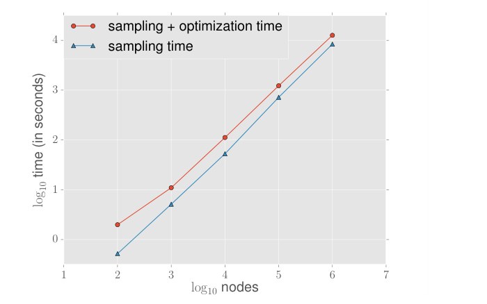
Figure 6: Scalability of node2vec on Erdos-Renyi graphs with an average degree of 10.
图 6:node2vec 在平均度为 10 的 Erdős–Rényi 图上的可扩展性。
To test for scalability, we learn node representations using node2vec with default parameter values for Erdos-Renyi graphs with increasing sizes from 100 to 1,000,000 nodes and constant average degree of 10. In Figure 6, we empirically observe that node2vec scales linearly with increase in number of nodes generating representations for one million nodes in less than four hours. The sampling procedure comprises of preprocessing for computing transition probabilities for our walk (negligibly small) and simulation of random walks. The optimization phase is made efficient using negative sampling [22] and asynchronous SGD [26].
为了测试可扩展性,我们用默认参数值,在规模从 100 增加到 1,000,000 个节点、平均度固定为 10 的 Erdős–Rényi 图上,用 node2vec 学习节点表示。在图 6 中,我们经验地观察到,node2vec 随节点数目增加呈线性扩展,为一百万个节点生成表示用了不到四小时。抽样过程包括为游走计算转移概率的预处理(可忽略地小)以及随机游走的模拟。优化阶段通过负采样 [22] 和异步 SGD [26] 变得高效。
Many ideas from prior work serve as useful pointers in making the sampling procedure computationally efficient. We showed how random walks, also used in DeepWalk [24], allow the sampled nodes to be reused as neighborhoods for different source nodes appearing in the walk. Alias sampling allows our walks to generalize to weighted networks, with little preprocessing [28]. Though we are free to set the search parameters based on the underlying task and domain at no additional cost, learning the best settings of our search parameters adds an overhead. However, as our experiments confirm, this overhead is minimal since node2vec is semi-supervised and hence, can learn these parameters efficiently with very little labeled data.
先前工作中的许多想法,为使抽样过程在计算上高效提供了有用线索。我们说明了随机游走(DeepWalk [24] 也使用)如何允许把抽到的节点复用为游走中出现的不同源节点的邻域。Alias sampling 使我们的游走能够推广到带权网络,只需很少的预处理 [28]。尽管我们可以按底层任务和领域自由设置搜索参数而不增加额外代价,但学习搜索参数的最佳设置会带来一些开销。不过,正如我们的实验所证实的,这一开销很小,因为 node2vec 是半监督的,因而可以用极少的带标签数据高效地学习这些参数。
4.7 Link prediction
4.7 链接预测
In link prediction, we are given a network with a certain fraction of edges removed, and we would like to predict these missing edges. We generate the labeled dataset of edges as follows: To obtain positive examples, we remove 50% of edges chosen randomly from the network while ensuring that the residual network obtained after the edge removals is connected, and to generate negative examples, we randomly sample an equal number of node pairs from the network which have no edge connecting them.
在链接预测中,我们得到一个被去掉了一定比例边的网络,并希望预测这些缺失的边。我们按如下方式生成带标签的边数据集:为得到正例,我们从网络中随机选取并去掉 50% 的边,同时确保去边后得到的残差网络仍然连通;为生成负例,我们从网络中随机抽取同等数量、之间没有边相连的节点对。
Since none of feature learning algorithms have been previously used for link prediction, we additionally evaluate node2vec against some popular heuristic scores that achieve good performance in link prediction. The scores we consider are defined in terms of the neighborhood sets of the nodes constituting the pair (see Table 3). We test our benchmarks on the following datasets:
由于这些特征学习算法先前都未被用于链接预测,我们还把 node2vec 与一些在链接预测上表现良好的流行启发式分数做了比较。我们考虑的分数是用构成该对的节点的邻域集合来定义的(见表 3)。我们在下列数据集上测试对照方法:
- • Facebook [14]: In the Facebook network, nodes represent users, and edges represent a friendship relation between any two users. The network has 4,039 nodes and 88,234 edges.
- • Facebook [14]:在 Facebook 网络中,节点表示用户,边表示任意两名用户之间的好友关系。该网络有 4,039 个节点和 88,234 条边。
- • Protein-Protein Interactions (PPI) [5]: In the PPI network for Homo Sapiens, nodes represent proteins, and an edge indicates a biological interaction between a pair of proteins. The network has 19,706 nodes and 390,633 edges.
- • 蛋白质相互作用(PPI) [5]:在智人的 PPI 网络中,节点表示蛋白质,边表示一对蛋白质之间的生物学相互作用。该网络有 19,706 个节点和 390,633 条边。
- • arXiv ASTRO-PH [14]: This is a collaboration network generated from papers submitted to the e-print arXiv where nodes represent scientists, and an edge is present between two scientists if they have collaborated in a paper. The network has 18,722 nodes and 198,110 edges.
- • arXiv ASTRO-PH [14]:这是从提交到电子预印本 arXiv 的论文生成的合作网络,节点表示科学家,若两名科学家曾在一篇论文中合作则有边。该网络有 18,722 个节点和 198,110 条边。
Experimental results. We summarize our results for link prediction in Table 4. The best and parameter settings for each node2vec entry are omitted for ease of presentation. A general observation we can draw from the results is that the learned feature representations for node pairs significantly outperform the heuristic benchmark scores with node2vec achieving the best AUC improvement on 12.6% on the arXiv dataset over the best performing baseline (Adamic-Adar [1]).
实验结果。 我们在表 4 中概括链接预测的结果。每个 node2vec 条目最好的 和 参数设置,为便于展示而省略。从结果可以得出的一个一般观察是:为节点对学到的特征表示显著超过启发式对照分数,node2vec 在 arXiv 数据集上相对表现最好的基线(Adamic-Adar [1])取得了 12.6% 的最佳 AUC 改进。
| Score | Definition |
|---|---|
| Common Neighbors | |
| Jaccard’s Coefficient | |
| Adamic-Adar Score | |
| Preferential Attachment |
Table 3: Link prediction heuristic scores for node pair with immediate neighbor sets and respectively.
| 分数 | 定义 |
|---|---|
| 共同邻居 | |
| Jaccard 系数 | |
| Adamic-Adar 分数 | |
| 优先连接 |
表 3:节点对 的链接预测启发式分数,其直接邻居集合分别为 和 。
Amongst the feature learning algorithms, node2vec outperforms both DeepWalk and LINE in all networks with gain up to 3.8% and 6.5% respectively in the AUC scores for the best possible choices of the binary operator for each algorithm. When we look at operators individually (Table 1), node2vec outperforms DeepWalk and LINE barring a couple of cases involving the Weighted-L1 and Weighted-L2 operators in which LINE performs better. Overall, the Hadamard operator when used with node2vec is highly stable and gives the best performance on average across all networks.
在特征学习算法之中,node2vec 在所有网络上都超过 DeepWalk 和 LINE,在各算法所能选择的最好二元算子下,AUC 分数的增益分别最高达 3.8% 和 6.5%。当我们逐个观察算子时(表 1),除了加权 和加权 算子的个别情形 LINE 更好之外,node2vec 都超过 DeepWalk 和 LINE。总体而言,Hadamard 算子与 node2vec 一起使用时高度稳定,并在所有网络上平均给出最好的性能。
| Op | Algorithm | Dataset | ||
|---|---|---|---|---|
| PPI | arXiv | |||
| Common Neighbors | 0.8100 | 0.7142 | 0.8153 | |
| Jaccard’s Coefficient | 0.8880 | 0.7018 | 0.8067 | |
| Adamic-Adar | 0.8289 | 0.7126 | 0.8315 | |
| Pref. Attachment | 0.7137 | 0.6670 | 0.6996 | |
| Spectral Clustering | 0.5960 | 0.6588 | 0.5812 | |
| (a) | DeepWalk | 0.7238 | 0.6923 | 0.7066 |
| LINE | 0.7029 | 0.6330 | 0.6516 | |
| node2vec | 0.7266 | 0.7543 | 0.7221 | |
| Spectral Clustering | 0.6192 | 0.4920 | 0.5740 | |
| (b) | DeepWalk | 0.9680 | 0.7441 | 0.9340 |
| LINE | 0.9490 | 0.7249 | 0.8902 | |
| node2vec | 0.9680 | 0.7719 | 0.9366 | |
| Spectral Clustering | 0.7200 | 0.6356 | 0.7099 | |
| (c) | DeepWalk | 0.9574 | 0.6026 | 0.8282 |
| LINE | 0.9483 | 0.7024 | 0.8809 | |
| node2vec | 0.9602 | 0.6292 | 0.8468 | |
| Spectral Clustering | 0.7107 | 0.6026 | 0.6765 | |
| (d) | DeepWalk | 0.9584 | 0.6118 | 0.8305 |
| LINE | 0.9460 | 0.7106 | 0.8862 | |
| node2vec | 0.9606 | 0.6236 | 0.8477 |
Table 4: Area Under Curve (AUC) scores for link prediction. Comparison with popular baselines and embedding based methods bootstapped using binary operators: (a) Average, (b) Hadamard, (c) Weighted-L1, and (d) Weighted-L2 (See Table 1 for definitions).
| 算子 | 算法 | 数据集 | ||
|---|---|---|---|---|
| PPI | arXiv | |||
| 共同邻居 | 0.8100 | 0.7142 | 0.8153 | |
| Jaccard 系数 | 0.8880 | 0.7018 | 0.8067 | |
| Adamic-Adar | 0.8289 | 0.7126 | 0.8315 | |
| 优先连接 | 0.7137 | 0.6670 | 0.6996 | |
| 谱聚类 | 0.5960 | 0.6588 | 0.5812 | |
| (a) | DeepWalk | 0.7238 | 0.6923 | 0.7066 |
| LINE | 0.7029 | 0.6330 | 0.6516 | |
| node2vec | 0.7266 | 0.7543 | 0.7221 | |
| 谱聚类 | 0.6192 | 0.4920 | 0.5740 | |
| (b) | DeepWalk | 0.9680 | 0.7441 | 0.9340 |
| LINE | 0.9490 | 0.7249 | 0.8902 | |
| node2vec | 0.9680 | 0.7719 | 0.9366 | |
| 谱聚类 | 0.7200 | 0.6356 | 0.7099 | |
| (c) | DeepWalk | 0.9574 | 0.6026 | 0.8282 |
| LINE | 0.9483 | 0.7024 | 0.8809 | |
| node2vec | 0.9602 | 0.6292 | 0.8468 | |
| 谱聚类 | 0.7107 | 0.6026 | 0.6765 | |
| (d) | DeepWalk | 0.9584 | 0.6118 | 0.8305 |
| LINE | 0.9460 | 0.7106 | 0.8862 | |
| node2vec | 0.9606 | 0.6236 | 0.8477 |
表 4:链接预测的曲线下面积(AUC)分数。与流行基线以及用二元算子组合得到的嵌入方法的比较:(a)平均,(b)Hadamard,(c)加权 ,以及(d)加权 (定义见表 1)。
5 Discussion and Conclusion
5 讨论与结论
In this paper, we studied feature learning in networks as a search-based optimization problem. This perspective gives us multiple advantages. It can explain classic search strategies on the basis of the exploration-exploitation trade-off. Additionally, it provides a degree of interpretability to the learned representations when applied for a prediction task. For instance, we observed that BFS can explore only limited neighborhoods. This makes BFS suitable for characterizing structural equivalences in network that rely on the immediate local structure of nodes. On the other hand, DFS can freely explore network neighborhoods which is important in discovering homophilous communities at the cost of high variance.
在本文中,我们把网络中的特征学习作为基于搜索的优化问题来研究。这一视角给我们带来多方面的好处。它可以在探索–利用权衡的基础上解释经典搜索策略。此外,当把学到的表示用于预测任务时,它还提供了一定程度的可解释性。例如,我们观察到 BFS 只能探索有限的邻域。这使得 BFS 适合刻画依赖节点直接局部结构的网络结构等价。另一方面,DFS 可以自由探索网络邻域,这对发现同配性社区很重要,代价则是高方差。
Both DeepWalk and LINE can be seen as rigid search strategies over networks. DeepWalk [24] proposes search using uniform random walks. The obvious limitation with such a strategy is that it gives us no control over the explored neighborhoods. LINE [28] proposes primarily a breadth-first strategy, sampling nodes and optimizing the likelihood independently over only 1-hop and 2-hop neighbors. The effect of such an exploration is easier to characterize, but it is restrictive and provides no flexibility in exploring nodes at further depths. In contrast, the search strategy in node2vec is both flexible and controllable exploring network neighborhoods through parameters and . While these search parameters have intuitive interpretations, we obtain best results on complex networks when we can learn them directly from data. From a practical standpoint, node2vec is scalable and robust to perturbations.
DeepWalk 和 LINE 都可以视为网络上的僵硬搜索策略。DeepWalk [24] 提出用均匀随机游走做搜索。这种策略的明显限制是,它对我们所探索的邻域没有任何控制。LINE [28] 主要提出一种广度优先策略,只在 1 跳和 2 跳邻居上独立地抽样节点并优化似然。这种探索的效果更容易刻画,但它是受限的,在探索更深处的节点时并不提供灵活性。相对地,node2vec 中的搜索策略既灵活又可控,通过参数 和 探索网络邻域。尽管这些搜索参数具有直观解释,但在复杂网络上,当我们能够直接从数据中学习它们时,会得到最好的结果。从实用角度看,node2vec 是可扩展的,并且对扰动稳健。
We showed how extensions of node embeddings to link prediction outperform popular heuristic scores designed specifically for this task. Our method permits additional binary operators beyond those listed in Table 1. As a future work, we would like to explore the reasons behind the success of Hadamard operator over others, as well as establish interpretable equivalence notions for edges based on the search parameters. Future extensions of node2vec could involve networks with special structure such as heterogeneous information networks, networks with explicit domain features for nodes and edges and signed-edge networks. Continuous feature representations are the backbone of many deep learning algorithms, and it would be interesting to use node2vec representations as building blocks for end-to-end deep learning on graphs.
我们表明,把节点嵌入扩展到链接预测,可以超过专门为这一任务设计的流行启发式分数。我们的方法还允许使用表 1 所列之外的其他二元算子。作为未来工作,我们希望探索 Hadamard 算子相对其他算子取得成功的原因,并基于搜索参数为边建立可解释的等价概念。node2vec 未来的扩展可以涉及具有特殊结构的网络,例如异构信息网络、节点和边带有显式领域特征的网络,以及带符号边的网络。连续特征表示是许多深度学习算法的骨干,把 node2vec 表示用作图上端到端深度学习的构建模块,将会很有意思。
Acknowledgements. We are thankful to Austin Benson, Will Hamilton, Rok Sosič, Marinka Žitnik as well as the anonymous reviewers for their helpful comments. This research has been supported in part by NSF CNS-1010921, IIS-1149837, NIH BD2K, ARO MURI, DARPA XDATA, DARPA SIMPLEX, Stanford Data Science Initiative, Boeing, Lightspeed, SAP, and Volkswagen.
致谢。 我们感谢 Austin Benson、Will Hamilton、Rok Sosič、Marinka Žitnik 以及匿名审稿人提出的有益意见。本研究部分得到 NSF CNS-1010921、IIS-1149837、NIH BD2K、ARO MURI、DARPA XDATA、DARPA SIMPLEX、斯坦福数据科学倡议、Boeing、Lightspeed、SAP 和 Volkswagen 的支持。
References
参考文献
[1] L. A. Adamic and E. Adar. Friends and neighbors on the web. Social networks , 25(3):211–230, 2003.
[2] L. Backstrom and J. Leskovec. Supervised random walks: predicting and recommending links in social networks. In WSDM , 2011.
[3] M. Belkin and P. Niyogi. Laplacian eigenmaps and spectral techniques for embedding and clustering. In NIPS , 2001.
[4] Y. Bengio, A. Courville, and P. Vincent. Representation learning: A review and new perspectives. IEEE TPAMI , 35(8):1798–1828, 2013.
[5] B.-J. Breitkreutz, C. Stark, T. Reguly, L. Boucher, A. Breitkreutz, M. Livstone, R. Oughtred, D. H. Lackner, J. Bähler, V. Wood, et al. The BioGRID interaction database. Nucleic acids research , 36:D637–D640, 2008.
[6] S. Cao, W. Lu, and Q. Xu. GraRep: Learning Graph Representations with global structural information. In CIKM , 2015.
[7] S. Fortunato. Community detection in graphs. Physics Reports , 486(3-5):75 – 174, 2010.
[8] B. Gallagher and T. Eliassi-Rad. Leveraging label-independent features for classification in sparsely labeled networks: An empirical study. In Lecture Notes in Computer Science: Advances in Social Network Mining and Analysis . Springer, 2009.
[9] Z. S. Harris. Word. Distributional Structure , 10(23):146–162, 1954.
[10] K. Henderson, B. Gallagher, T. Eliassi-Rad, H. Tong, S. Basu, L. Akoglu, D. Koutra, C. Faloutsos, and L. Li. RolX: structural role extraction & mining in large graphs. In KDD , 2012.
[11] K. Henderson, B. Gallagher, L. Li, L. Akoglu, T. Eliassi-Rad, H. Tong, and C. Faloutsos. It’s who you know: graph mining using recursive structural features. In KDD , 2011.
[12] P. D. Hoff, A. E. Raftery, and M. S. Handcock. Latent space approaches to social network analysis. J. of the American Statistical Association , 2002.
[13] D. E. Knuth. The Stanford GraphBase: a platform for combinatorial computing , volume 37. Addison-Wesley Reading, 1993.
[14] J. Leskovec and A. Krevl. SNAP Datasets: Stanford large network dataset collection. http://snap.stanford.edu/data , June 2014.
[15] K. Li, J. Gao, S. Guo, N. Du, X. Li, and A. Zhang. LRBM: A restricted boltzmann machine based approach for representation learning on linked data. In ICDM , 2014.
[16] X. Li, N. Du, H. Li, K. Li, J. Gao, and A. Zhang. A deep learning approach to link prediction in dynamic networks. In ICDM , 2014.
[17] Y. Li, D. Tarlow, M. Brockschmidt, and R. Zemel. Gated graph sequence neural networks. In ICLR , 2016.
[18] D. Liben-Nowell and J. Kleinberg. The link-prediction problem for social networks. J. of the American society for information science and technology , 58(7):1019–1031, 2007.
[19] A. Liberzon, A. Subramanian, R. Pinchback, H. Thorvaldsdóttir, P. Tamayo, and J. P. Mesirov. Molecular signatures database (MSigDB) 3.0. Bioinformatics , 27(12):1739–1740, 2011.
[20] M. Mahoney. Large text compression benchmark. www.mattmahoney.net/dc/textdata , 2011.
[21] T. Mikolov, K. Chen, G. Corrado, and J. Dean. Efficient estimation of word representations in vector space. In ICLR , 2013.
[22] T. Mikolov, I. Sutskever, K. Chen, G. S. Corrado, and J. Dean. Distributed representations of words and phrases and their compositionality. In NIPS , 2013.
[23] J. Pennington, R. Socher, and C. D. Manning. GloVe: Global vectors for word representation. In EMNLP , 2014.
[24] B. Perozzi, R. Al-Rfou, and S. Skiena. DeepWalk: Online learning of social representations. In KDD , 2014.
[25] P. Radivojac, W. T. Clark, T. R. Oron, A. M. Schnoes, T. Wittkop, A. Sokolov, K. Graim, C. Funk, Verspoor, et al. A large-scale evaluation of computational protein function prediction. Nature methods , 10(3):221–227, 2013.
[26] B. Recht, C. Re, S. Wright, and F. Niu. Hogwild!: A lock-free approach to parallelizing stochastic gradient descent. In NIPS , 2011.
[27] S. T. Roweis and L. K. Saul. Nonlinear dimensionality reduction by locally linear embedding. Science , 290(5500):2323–2326, 2000.
[28] J. Tang, M. Qu, M. Wang, M. Zhang, J. Yan, and Q. Mei. LINE: Large-scale Information Network Embedding. In WWW , 2015.
[29] L. Tang and H. Liu. Leveraging social media networks for classification. Data Mining and Knowledge Discovery , 23(3):447–478, 2011.
[30] J. B. Tenenbaum, V. De Silva, and J. C. Langford. A global geometric framework for nonlinear dimensionality reduction. Science , 290(5500):2319–2323, 2000.
[31] F. Tian, B. Gao, Q. Cui, E. Chen, and T.-Y. Liu. Learning deep representations for graph clustering. In AAAI , 2014.
[32] K. Toutanova, D. Klein, C. D. Manning, and Y. Singer. Feature-rich part-of-speech tagging with a cyclic dependency network. In NAACL , 2003.
[33] G. Tsoumakas and I. Katakis. Multi-label classification: An overview. Dept. of Informatics, Aristotle University of Thessaloniki, Greece , 2006.
[34] A. Vazquez, A. Flammini, A. Maritan, and A. Vespignani. Global protein function prediction from protein-protein interaction networks. Nature biotechnology , 21(6):697–700, 2003.
[35] S. Yan, D. Xu, B. Zhang, H.-J. Zhang, Q. Yang, and S. Lin. Graph embedding and extensions: a general framework for dimensionality reduction. IEEE TPAMI , 29(1):40–51, 2007.
[36] J. Yang and J. Leskovec. Overlapping communities explain core-periphery organization of networks. Proceedings of the IEEE , 102(12):1892–1902, 2014.
[37] S.-H. Yang, B. Long, A. Smola, N. Sadagopan, Z. Zheng, and H. Zha. Like like alike: joint friendship and interest propagation in social networks. In WWW , 2011.
[38] R. Zafarani and H. Liu. Social computing data repository at ASU, 2009.
[39] S. Zhai and Z. Zhang. Dropout training of matrix factorization and autoencoder for link prediction in sparse graphs. In SDM , 2015.