Neural Tangent Kernel: Convergence and Generalization in Neural Networks | AGIDaily
AGI Daily
资讯日报词条论文人物新创
返回论文列表
摘要1 引言1.1 贡献2 神经网络3 核梯度3.1 随机函数逼近4 神经正切核4.1 初始化4.2 训练5 最小二乘回归6 数值实验6.1 NTK 的收敛6.2 核回归6.3 沿主成分的收敛7 结论致谢参考文献附录 A 附录A.1 初始化时的渐近Proposition 1.证明.Theorem 1.证明.A.2 训练中的渐近Theorem 2.证明.Lemma 1.A.3 训练中的先验控制Lemma 1.证明.A.4 $\Theta^{(L)}{\infty}$ 的正定性Proposition 2.Lemma 2(Lemma 12(a) in suppl. mat. of [20]).Theorem 3.命题 2 的证明.Remark 5.
返回论文列表
目录

Neural Tangent Kernel: Convergence and Generalization in Neural Networks

收录于 NeurIPS 2018 会议论文;Advances in Neural Information Processing Systems 31;arXiv:1806.07572被引 1,840 次
打开论文来源

Neural Tangent Kernel: Convergence and Generalization in Neural Networks

Arthur Jacot
École Polytechnique Fédérale de Lausanne
arthur.jacot@netopera.net

Franck Gabriel
Imperial College London and École Polytechnique Fédérale de Lausanne
franckrgabriel@gmail.com

Clément Hongler
École Polytechnique Fédérale de Lausanne
clement.hongler@gmail.com

32nd Conference on Neural Information Processing Systems (NeurIPS 2018), Montréal, Canada.

Abstract

摘要

At initialization, artificial neural networks (ANNs) are equivalent to Gaussian processes in the infinite-width limit (12; 9), thus connecting them to kernel methods. We prove that the evolution of an ANN during training can also be described by a kernel: during gradient descent on the parameters of an ANN, the network function fθf_{\theta}fθ​ (which maps input vectors to output vectors) follows the kernel gradient of the functional cost (which is convex, in contrast to the parameter cost) w.r.t. a new kernel: the Neural Tangent Kernel (NTK). This kernel is central to describe the generalization features of ANNs. While the NTK is random at initialization and varies during training, in the infinite-width limit it converges to an explicit limiting kernel and it stays constant during training. This makes it possible to study the training of ANNs in function space instead of parameter space. Convergence of the training can then be related to the positive-definiteness of the limiting NTK.

在初始化时,人工神经网络(ANN)在无限宽极限下等价于高斯过程(12; 9),从而与核方法联系起来。我们证明,ANN 在训练中的演化也可以用一个核来描述:在网络参数上做梯度下降时,网络函数 fθf_{\theta}fθ​(把输入向量映到输出向量)会沿着泛函代价(它是凸的,与参数代价不同)相对于一个新核——神经正切核(Neural Tangent Kernel,NTK)——的核梯度前进。这一核对于刻画 ANN 的泛化性质是中心性的。NTK 在初始化时是随机的,并会在训练中变化;但在无限宽极限下,它收敛到一个可以显式写出的极限核,并且在训练过程中保持不变。于是我们可以在函数空间而不是参数空间里研究 ANN 的训练。训练能否收敛,也可以与极限 NTK 的正定性联系起来。

We then focus on the setting of least-squares regression and show that in the infinite-width limit, the network function fθf_{\theta}fθ​ follows a linear differential equation during training. The convergence is fastest along the largest kernel principal components of the input data with respect to the NTK, hence suggesting a theoretical motivation for early stopping.

接着我们聚焦于最小二乘回归,并证明在无限宽极限下,网络函数 fθf_{\theta}fθ​ 在训练中服从一个线性微分方程。收敛沿相对于 NTK 的最大核主成分最快,从而为早停提供了一种理论上的动机。

Finally we study the NTK numerically, observe its behavior for wide networks, and compare it to the infinite-width limit.

最后我们从数值上研究 NTK,观察它在宽网络上的行为,并与无限宽极限加以比较。

1 Introduction

1 引言

Artificial neural networks (ANNs) have achieved impressive results in numerous areas of machine learning. While it has long been known that ANNs can approximate any function with sufficiently many hidden neurons (7; 10), it is not known what the optimization of ANNs converges to. Indeed the loss surface of neural networks optimization problems is highly non-convex: it has a high number of saddle points which may slow down the convergence (4). A number of results (3; 13; 14) suggest that for wide enough networks, there are very few “bad” local minima, i.e. local minima with much higher cost than the global minimum. More recently, the investigation of the geometry of the loss landscape at initialization has been the subject of a precise study (8). The analysis of the dynamics of training in the large-width limit for shallow networks has seen recent progress as well (11). To the best of the authors knowledge, the dynamics of deep networks has however remained an open problem until the present paper: see the contributions section below.

人工神经网络(ANN)已在机器学习的许多领域取得令人瞩目的结果。虽然人们早已知道,只要隐神经元足够多,ANN 可以逼近任意函数(7; 10),但 ANN 的优化会收敛到什么,仍不清楚。神经网络优化问题的损失曲面高度非凸:其中有大量鞍点,可能拖慢收敛(4)。一些结果(3; 13; 14)表明,对足够宽的网络而言,“很差”的局部极小很少,也就是代价远高于全局最小的局部极小很少。更近一些,初始化处损失地貌的几何已有精确研究(8)。浅层网络在大宽度极限下的训练动力学也有新的进展(11)。据作者所知,直到本文之前,深层网络的动力学仍是未解决问题:见下文的贡献一节。

A particularly mysterious feature of ANNs is their good generalization properties in spite of their usual over-parametrization (16). It seems paradoxical that a reasonably large neural network can fit random labels, while still obtaining good test accuracy when trained on real data (19). It can be noted that in this case, kernel methods have the same properties (1).

ANN 一个特别费解的特点是:尽管通常过参数化,它们仍有很好的泛化(16)。一个规模合理的网络既能拟合随机标签,在真实数据上训练时又能得到不错的测试准确率,这看起来自相矛盾(19)。可以指出,在这种情形下,核方法也有同样的性质(1)。

In the infinite-width limit, ANNs have a Gaussian distribution described by a kernel (12; 9). These kernels are used in Bayesian inference or Support Vector Machines, yielding results comparable to ANNs trained with gradient descent (9; 2). We will see that in the same limit, the behavior of ANNs during training is described by a related kernel, which we call the neural tangent network (NTK).

在无限宽极限下,ANN 具有由一个核描述的高斯分布(12; 9)。这些核被用于贝叶斯推断或支持向量机,得到的结果可与用梯度下降训练的 ANN 相比(9; 2)。我们将看到,在同一极限下,ANN 在训练中的行为由一个相关的核描述,我们称之为 neural tangent network(NTK)。

1.1 Contribution

1.1 贡献

We study the network function fθf_{\theta}fθ​ of an ANN, which maps an input vector to an output vector, where θ\thetaθ is the vector of the parameters of the ANN. In the limit as the widths of the hidden layers tend to infinity, the network function at initialization, fθf_{\theta}fθ​ converges to a Gaussian distribution (12; 9).

我们研究 ANN 的网络函数 fθf_{\theta}fθ​:它把输入向量映到输出向量,其中 θ\thetaθ 是 ANN 的参数向量。当隐层宽度趋于无穷时,初始化处的网络函数 fθf_{\theta}fθ​ 收敛到高斯分布(12; 9)。

In this paper, we investigate fully connected networks in this infinite-width limit, and describe the dynamics of the network function fθf_{\theta}fθ​ during training:

本文在这一无限宽极限下研究全连接网络,并描述网络函数 fθf_{\theta}fθ​ 在训练中的动力学:

  • During gradient descent, we show that the dynamics of fθf_{\theta}fθ​ follows that of the so-called kernel gradient descent in function space with respect to a limiting kernel, which only depends on the depth of the network, the choice of nonlinearity and the initialization variance.
  • 在梯度下降中,我们证明 fθf_{\theta}fθ​ 的动力学与函数空间中相对于某个极限核的所谓核梯度下降一致;该极限核只依赖于网络深度、非线性的选取以及初始化方差。
  • The convergence properties of ANNs during training can then be related to the positive-definiteness of the infinite-width limit NTK. The values of the network function fθf_{\theta}fθ​ outside the training set is described by the NTK, which is crucial to understand how ANN generalize.
  • 于是,ANN 在训练中的收敛性质可以与无限宽极限 NTK 的正定性联系起来。训练集之外的网络函数 fθf_{\theta}fθ​ 取值由 NTK 描述,这对理解 ANN 如何泛化至关重要。
  • For a least-squares regression loss, the network function fθf_{\theta}fθ​ follows a linear differential equation in the infinite-width limit, and the eigenfunctions of the Jacobian are the kernel principal components of the input data. This shows a direct connection to kernel methods and motivates the use of early stopping to reduce overfitting in the training of ANNs.
  • 对最小二乘回归损失,网络函数 fθf_{\theta}fθ​ 在无限宽极限下服从线性微分方程,而雅可比的特征函数正是输入数据的核主成分。这显示了与核方法的直接联系,并为在 ANN 训练中用早停减轻过拟合提供了动机。
  • Finally we investigate these theoretical results numerically for an artificial dataset (of points on the unit circle) and for the MNIST dataset. In particular we observe that the behavior of wide ANNs is close to the theoretical limit.
  • 最后,我们在一个人造数据集(单位圆上的点)以及 MNIST 数据集上,从数值上考察这些理论结果。特别地,我们观察到宽 ANN 的行为接近理论极限。

2 Neural networks

2 神经网络

In this article, we consider fully-connected ANNs with layers numbered from 000 (input) to LLL (output), each containing n0,…,nLn_{0},\ldots,n_{L}n0​,…,nL​ neurons, and with a Lipschitz, twice differentiable nonlinearity function σ:R→R\sigma:\mathbb{R}\to\mathbb{R}σ:R→R, with bounded second derivative.1^{1}1

本文考虑全连接 ANN,层从 000(输入)编号到 LLL(输出),各层分别有 n0,…,nLn_{0},\ldots,n_{L}n0​,…,nL​ 个神经元,并带有一个 Lipschitz、二阶可微且二阶导数有界的非线性函数 σ:R→R\sigma:\mathbb{R}\to\mathbb{R}σ:R→R。1^{1}1

1^{1}1While these smoothness assumptions greatly simplify the proofs of our results, they do not seem to be strictly needed for the results to hold true.

1^{1}1这些光滑性假设大大简化了我们结果的证明,但结果成立似乎并不严格需要它们。

This paper focuses on the ANN realization function F(L):RP→FF^{(L)}:\mathbb{R}^{P}\to\mathcal{F}F(L):RP→F, mapping parameters θ\thetaθ to functions fθf_{\theta}fθ​ in a space F\mathcal{F}F. The dimension of the parameter space is P=∑ℓ=0L−1(nℓ+1)nℓ+1P=\sum_{\ell=0}^{L-1}(n_{\ell}+1)n_{\ell+1}P=∑ℓ=0L−1​(nℓ​+1)nℓ+1​: the parameters consist of the connection matrices W(ℓ)∈Rnℓ×nℓ+1W^{(\ell)}\in\mathbb{R}^{n_{\ell}\times n_{\ell+1}}W(ℓ)∈Rnℓ​×nℓ+1​ and bias vectors b(ℓ)∈Rnℓ+1b^{(\ell)}\in\mathbb{R}^{n_{\ell+1}}b(ℓ)∈Rnℓ+1​ for ℓ=0,…,L−1\ell=0,\ldots,L-1ℓ=0,…,L−1. In our setup, the parameters are initialized as iid Gaussians N(0,1)\mathcal{N}(0,1)N(0,1).

本文关注 ANN 的实现函数 F(L):RP→FF^{(L)}:\mathbb{R}^{P}\to\mathcal{F}F(L):RP→F,它把参数 θ\thetaθ 映到函数空间 F\mathcal{F}F 中的函数 fθf_{\theta}fθ​。参数空间的维数是 P=∑ℓ=0L−1(nℓ+1)nℓ+1P=\sum_{\ell=0}^{L-1}(n_{\ell}+1)n_{\ell+1}P=∑ℓ=0L−1​(nℓ​+1)nℓ+1​:参数由连接矩阵 W(ℓ)∈Rnℓ×nℓ+1W^{(\ell)}\in\mathbb{R}^{n_{\ell}\times n_{\ell+1}}W(ℓ)∈Rnℓ​×nℓ+1​ 和偏置向量 b(ℓ)∈Rnℓ+1b^{(\ell)}\in\mathbb{R}^{n_{\ell+1}}b(ℓ)∈Rnℓ+1​ 组成,其中 ℓ=0,…,L−1\ell=0,\ldots,L-1ℓ=0,…,L−1。在我们的设定里,参数初始化为独立同分布的高斯 N(0,1)\mathcal{N}(0,1)N(0,1)。

For a fixed distribution pinp^{\mathrm{in}}pin on the input space Rn0\mathbb{R}^{n_{0}}Rn0​, the function space F\mathcal{F}F is defined as {f:Rn0→RnL}\{f:\mathbb{R}^{n_{0}}\to\mathbb{R}^{n_{L}}\}{f:Rn0​→RnL​}. On this space, we consider the seminorm ∥⋅∥pin\|\cdot\|_{p^{\mathrm{in}}}∥⋅∥pin​, defined in terms of the bilinear form

对输入空间 Rn0\mathbb{R}^{n_{0}}Rn0​ 上的固定分布 pinp^{\mathrm{in}}pin,函数空间 F\mathcal{F}F 定义为 {f:Rn0→RnL}\{f:\mathbb{R}^{n_{0}}\to\mathbb{R}^{n_{L}}\}{f:Rn0​→RnL​}。在这个空间上,我们考虑半范数 ∥⋅∥pin\|\cdot\|_{p^{\mathrm{in}}}∥⋅∥pin​,它由下述双线性形式给出:

⟨f,g⟩pin=Ex∼pin[f(x)Tg(x)].\langle f,g\rangle_{p^{\mathrm{in}}}=\mathbb{E}_{x\sim p^{\mathrm{in}}}\big[f(x)^{T}g(x)\big].⟨f,g⟩pin​=Ex∼pin​[f(x)Tg(x)].

In this paper, we assume that the input distribution pinp^{\mathrm{in}}pin is the empirical distribution on a finite dataset x1,…,xNx_{1},\ldots,x_{N}x1​,…,xN​, i.e the sum of Dirac measures 1N∑i=0Nδxi\frac{1}{N}\sum_{i=0}^{N}\delta_{x_{i}}N1​∑i=0N​δxi​​.

本文假定输入分布 pinp^{\mathrm{in}}pin 是有限数据集 x1,…,xNx_{1},\ldots,x_{N}x1​,…,xN​ 上的经验分布,即 Dirac 测度之和 1N∑i=0Nδxi\frac{1}{N}\sum_{i=0}^{N}\delta_{x_{i}}N1​∑i=0N​δxi​​。

We define the network function by fθ(x):=α~(L)(x;θ)f_{\theta}(x):=\tilde{\alpha}^{(L)}(x;\theta)fθ​(x):=α~(L)(x;θ), where the functions α~(ℓ)(⋅;θ):Rn0→Rnℓ\tilde{\alpha}^{(\ell)}(\cdot;\theta):\mathbb{R}^{n_{0}}\to\mathbb{R}^{n_{\ell}}α~(ℓ)(⋅;θ):Rn0​→Rnℓ​ (called preactivations) and α(ℓ)(⋅;θ):Rn0→Rnℓ\alpha^{(\ell)}(\cdot;\theta):\mathbb{R}^{n_{0}}\to\mathbb{R}^{n_{\ell}}α(ℓ)(⋅;θ):Rn0​→Rnℓ​ (called activations) are defined from the 000-th to the LLL-th layer by:

我们把网络函数定义为 fθ(x):=α~(L)(x;θ)f_{\theta}(x):=\tilde{\alpha}^{(L)}(x;\theta)fθ​(x):=α~(L)(x;θ),其中函数 α~(ℓ)(⋅;θ):Rn0→Rnℓ\tilde{\alpha}^{(\ell)}(\cdot;\theta):\mathbb{R}^{n_{0}}\to\mathbb{R}^{n_{\ell}}α~(ℓ)(⋅;θ):Rn0​→Rnℓ​(称为预激活)和 α(ℓ)(⋅;θ):Rn0→Rnℓ\alpha^{(\ell)}(\cdot;\theta):\mathbb{R}^{n_{0}}\to\mathbb{R}^{n_{\ell}}α(ℓ)(⋅;θ):Rn0​→Rnℓ​(称为激活)从第 000 层到第 LLL 层由下式递归给出:

$$\begin{aligned}
\alpha^{(0)}(x;\theta) &= x, \
\tilde{\alpha}^{(\ell+1)}(x;\theta) &= \frac{1}{\sqrt{n_{\ell}}}W^{(\ell)}\alpha^{(\ell)}(x;\theta)+\beta b^{(\ell)}, \
\alpha^{(\ell)}(x;\theta) &= \sigma(\tilde{\alpha}^{(\ell)}(x;\theta)),
\end{aligned}$$

where the nonlinearity σ\sigmaσ is applied entrywise. The scalar β>0\beta>0β>0 is a parameter which allows us to tune the influence of the bias on the training.

其中非线性 σ\sigmaσ 按分量作用。标量 β>0\beta>0β>0 是一个参数,用来调节偏置对训练的影响。

Remark 1. Our definition of the realization function F(L)F^{(L)}F(L) slightly differs from the classical one. Usually, the factors 1nℓ\frac{1}{\sqrt{n_{\ell}}}nℓ​​1​ and the parameter β\betaβ are absent and the parameters are initialized using what is sometimes called LeCun initialization, taking Wij(ℓ)∼N(0,1nℓ)W^{(\ell)}_{ij}\sim\mathcal{N}(0,\frac{1}{n_{\ell}})Wij(ℓ)​∼N(0,nℓ​1​) and bj(ℓ)∼N(0,1)b^{(\ell)}_{j}\sim\mathcal{N}(0,1)bj(ℓ)​∼N(0,1) (or sometimes bj(ℓ)=0b^{(\ell)}_{j}=0bj(ℓ)​=0) to compensate. While the set of representable functions F(L)(RP)F^{(L)}(\mathbb{R}^{P})F(L)(RP) is the same for both parametrizations (with or without the factors 1nℓ\frac{1}{\sqrt{n_{\ell}}}nℓ​​1​ and β\betaβ), the derivatives of the realization function with respect to the connections ∂Wij(ℓ)F(L)\partial_{W^{(\ell)}_{ij}}F^{(L)}∂Wij(ℓ)​​F(L) and bias ∂bj(ℓ)F(L)\partial_{b^{(\ell)}_{j}}F^{(L)}∂bj(ℓ)​​F(L) are scaled by 1nℓ\frac{1}{\sqrt{n_{\ell}}}nℓ​​1​ and β\betaβ respectively in comparison to the classical parametrization.

注 1. 我们对实现函数 F(L)F^{(L)}F(L) 的定义与经典定义略有不同。通常没有因子 1nℓ\frac{1}{\sqrt{n_{\ell}}}nℓ​​1​ 和参数 β\betaβ,参数则用有时称为 LeCun 初始化的方式初始化,取 Wij(ℓ)∼N(0,1nℓ)W^{(\ell)}_{ij}\sim\mathcal{N}(0,\frac{1}{n_{\ell}})Wij(ℓ)​∼N(0,nℓ​1​),bj(ℓ)∼N(0,1)b^{(\ell)}_{j}\sim\mathcal{N}(0,1)bj(ℓ)​∼N(0,1)(有时也取 bj(ℓ)=0b^{(\ell)}_{j}=0bj(ℓ)​=0)来补偿。两种参数化(有或没有因子 1nℓ\frac{1}{\sqrt{n_{\ell}}}nℓ​​1​ 和 β\betaβ)所能表示的函数集合 F(L)(RP)F^{(L)}(\mathbb{R}^{P})F(L)(RP) 是相同的,但实现函数对连接的导数 ∂Wij(ℓ)F(L)\partial_{W^{(\ell)}_{ij}}F^{(L)}∂Wij(ℓ)​​F(L) 和对偏置的导数 ∂bj(ℓ)F(L)\partial_{b^{(\ell)}_{j}}F^{(L)}∂bj(ℓ)​​F(L),相对于经典参数化分别被缩放了 1nℓ\frac{1}{\sqrt{n_{\ell}}}nℓ​​1​ 和 β\betaβ。

The factors 1nℓ\frac{1}{\sqrt{n_{\ell}}}nℓ​​1​ are key to obtaining a consistent asymptotic behavior of neural networks as the widths of the hidden layers n1,…,nL−1n_{1},\ldots,n_{L-1}n1​,…,nL−1​ grow to infinity. However a side-effect of these factors is that they reduce greatly the influence of the connection weights during training when nℓn_{\ell}nℓ​ is large: the factor β\betaβ is introduced to balance the influence of the bias and connection weights. In our numerical experiments, we take β=0.1\beta=0.1β=0.1 and use a learning rate of 1.01.01.0, which is larger than usual, see Section 6. This gives a behaviour similar to that of a classical network of width 100100100 with a learning rate of 0.010.010.01.

因子 1nℓ\frac{1}{\sqrt{n_{\ell}}}nℓ​​1​ 是使神经网络在隐层宽度 n1,…,nL−1n_{1},\ldots,n_{L-1}n1​,…,nL−1​ 趋于无穷时具有一致渐近行为的关键。但这些因子的一个副作用是:当 nℓn_{\ell}nℓ​ 很大时,它们会大大削弱连接权重在训练中的影响;引入因子 β\betaβ,正是为了平衡偏置与连接权重的影响。在数值实验中,我们取 β=0.1\beta=0.1β=0.1,并用 1.01.01.0 的学习率,这比通常更大,见第 6 节。这给出的行为,类似于宽度为 100100100、学习率为 0.010.010.01 的经典网络。

3 Kernel gradient

3 核梯度

The training of an ANN consists in optimizing fθf_{\theta}fθ​ in the function space F\mathcal{F}F with respect to a functional cost C:F→RC:\mathcal{F}\to\mathbb{R}C:F→R, such as a regression or cross-entropy cost. Even for a convex functional cost CCC, the composite cost C∘F(L):RP→RC\circ F^{(L)}:\mathbb{R}^{P}\to\mathbb{R}C∘F(L):RP→R is in general highly non-convex (3). We will show that during training, the network function fθf_{\theta}fθ​ follows a descent along the kernel gradient with respect to the Neural Tangent Kernel (NTK) which we introduce in Section 4. This makes it possible to study the training of ANNs in the function space F\mathcal{F}F, on which the cost CCC is convex.

训练 ANN,就是在函数空间 F\mathcal{F}F 中相对某个泛函代价 C:F→RC:\mathcal{F}\to\mathbb{R}C:F→R(例如回归或交叉熵代价)优化 fθf_{\theta}fθ​。即便泛函代价 CCC 是凸的,复合代价 C∘F(L):RP→RC\circ F^{(L)}:\mathbb{R}^{P}\to\mathbb{R}C∘F(L):RP→R 一般仍高度非凸(3)。我们将证明,在训练中,网络函数 fθf_{\theta}fθ​ 沿着第 4 节引入的神经正切核(NTK)的核梯度下降。于是可以在函数空间 F\mathcal{F}F 中研究 ANN 的训练,而在这个空间上代价 CCC 是凸的。

A multi-dimensional kernel KKK is a function Rn0×Rn0→RnL×nL\mathbb{R}^{n_{0}}\times\mathbb{R}^{n_{0}}\to\mathbb{R}^{n_{L}\times n_{L}}Rn0​×Rn0​→RnL​×nL​, which maps any pair (x,x′)(x,x')(x,x′) to an nL×nLn_{L}\times n_{L}nL​×nL​-matrix such that K(x,x′)=K(x′,x)TK(x,x')=K(x',x)^{T}K(x,x′)=K(x′,x)T (equivalently KKK is a symmetric tensor in F⊗F\mathcal{F}\otimes\mathcal{F}F⊗F). Such a kernel defines a bilinear map on F\mathcal{F}F, taking the expectation over independent x,x′∼pinx,x'\sim p^{\mathrm{in}}x,x′∼pin:

一个多维核 KKK 是函数 Rn0×Rn0→RnL×nL\mathbb{R}^{n_{0}}\times\mathbb{R}^{n_{0}}\to\mathbb{R}^{n_{L}\times n_{L}}Rn0​×Rn0​→RnL​×nL​,它把任意一对 (x,x′)(x,x')(x,x′) 映到一个 nL×nLn_{L}\times n_{L}nL​×nL​ 矩阵,并满足 K(x,x′)=K(x′,x)TK(x,x')=K(x',x)^{T}K(x,x′)=K(x′,x)T(等价地说,KKK 是 F⊗F\mathcal{F}\otimes\mathcal{F}F⊗F 中的对称张量)。这样的核在 F\mathcal{F}F 上定义一个双线性映射,期望对独立的 x,x′∼pinx,x'\sim p^{\mathrm{in}}x,x′∼pin 来取:

⟨f,g⟩K:=Ex,x′∼pin[f(x)TK(x,x′)g(x′)].\langle f,g\rangle_{K}:=\mathbb{E}_{x,x'\sim p^{\mathrm{in}}}\big[f(x)^{T}K(x,x')g(x')\big].⟨f,g⟩K​:=Ex,x′∼pin​[f(x)TK(x,x′)g(x′)].

The kernel KKK is positive definite with respect to ∥⋅∥pin\|\cdot\|_{p^{\mathrm{in}}}∥⋅∥pin​ if ∥f∥pin>0  ⟹  ∥f∥K>0\|f\|_{p^{\mathrm{in}}}>0\implies\|f\|_{K}>0∥f∥pin​>0⟹∥f∥K​>0.

若 ∥f∥pin>0  ⟹  ∥f∥K>0\|f\|_{p^{\mathrm{in}}}>0\implies\|f\|_{K}>0∥f∥pin​>0⟹∥f∥K​>0,则称核 KKK 相对于 ∥⋅∥pin\|\cdot\|_{p^{\mathrm{in}}}∥⋅∥pin​ 是正定的。

We denote by F∗\mathcal{F}^{*}F∗ the dual of F\mathcal{F}F with respect to pinp^{\mathrm{in}}pin, i.e. the set of linear forms μ:F→R\mu:\mathcal{F}\to\mathbb{R}μ:F→R of the form μ=⟨d,⋅⟩pin\mu=\langle d,\cdot\rangle_{p^{\mathrm{in}}}μ=⟨d,⋅⟩pin​ for some d∈Fd\in\mathcal{F}d∈F. Two elements of F\mathcal{F}F define the same linear form if and only if they are equal on the data. The constructions in the paper do not depend on the element d∈Fd\in\mathcal{F}d∈F chosen in order to represent μ\muμ as ⟨d,⋅⟩pin\langle d,\cdot\rangle_{p^{\mathrm{in}}}⟨d,⋅⟩pin​. Using the fact that the partial application of the kernel Ki,⋅(x,⋅)K_{i,\cdot}(x,\cdot)Ki,⋅​(x,⋅) is a function in F\mathcal{F}F, we can define a map ΦK:F∗→F\Phi_{K}:\mathcal{F}^{*}\to\mathcal{F}ΦK​:F∗→F mapping a dual element μ=⟨d,⋅⟩pin\mu=\langle d,\cdot\rangle_{p^{\mathrm{in}}}μ=⟨d,⋅⟩pin​ to the function fμ=ΦK(μ)f_{\mu}=\Phi_{K}(\mu)fμ​=ΦK​(μ) with values:

我们把 F\mathcal{F}F 相对于 pinp^{\mathrm{in}}pin 的对偶记作 F∗\mathcal{F}^{*}F∗,也就是形如 μ=⟨d,⋅⟩pin\mu=\langle d,\cdot\rangle_{p^{\mathrm{in}}}μ=⟨d,⋅⟩pin​(对某个 d∈Fd\in\mathcal{F}d∈F)的线性型 μ:F→R\mu:\mathcal{F}\to\mathbb{R}μ:F→R 的集合。F\mathcal{F}F 中两个元素定义同一个线性型,当且仅当它们在数据上相等。文中的构造不依赖于为把 μ\muμ 写成 ⟨d,⋅⟩pin\langle d,\cdot\rangle_{p^{\mathrm{in}}}⟨d,⋅⟩pin​ 而选取的那个 d∈Fd\in\mathcal{F}d∈F。利用核的偏应用 Ki,⋅(x,⋅)K_{i,\cdot}(x,\cdot)Ki,⋅​(x,⋅) 是 F\mathcal{F}F 中的函数,我们可以定义映射 ΦK:F∗→F\Phi_{K}:\mathcal{F}^{*}\to\mathcal{F}ΦK​:F∗→F,它把对偶元 μ=⟨d,⋅⟩pin\mu=\langle d,\cdot\rangle_{p^{\mathrm{in}}}μ=⟨d,⋅⟩pin​ 映到函数 fμ=ΦK(μ)f_{\mu}=\Phi_{K}(\mu)fμ​=ΦK​(μ),其取值为:

fμ,i(x)=μ Ki,⋅(x,⋅)=⟨d,Ki,⋅(x,⋅)⟩pin.f_{\mu,i}(x)=\mu\,K_{i,\cdot}(x,\cdot)=\langle d,K_{i,\cdot}(x,\cdot)\rangle_{p^{\mathrm{in}}}.fμ,i​(x)=μKi,⋅​(x,⋅)=⟨d,Ki,⋅​(x,⋅)⟩pin​.

For our setup, which is that of a finite dataset x1,…,xN∈Rn0x_{1},\ldots,x_{N}\in\mathbb{R}^{n_{0}}x1​,…,xN​∈Rn0​, the cost functional CCC only depends on the values of f∈Ff\in\mathcal{F}f∈F at the data points. As a result, the (functional) derivative of the cost CCC at a point f0∈Ff_{0}\in\mathcal{F}f0​∈F can be viewed as an element of F∗\mathcal{F}^{*}F∗, which we write ∂finC∣f0\partial^{\mathrm{in}}_{f}C|_{f_{0}}∂fin​C∣f0​​. We denote by d∣f0∈Fd|_{f_{0}}\in\mathcal{F}d∣f0​​∈F, a corresponding dual element, such that ∂finC∣f0=⟨d∣f0,⋅⟩pin\partial^{\mathrm{in}}_{f}C|_{f_{0}}=\langle d|_{f_{0}},\cdot\rangle_{p^{\mathrm{in}}}∂fin​C∣f0​​=⟨d∣f0​​,⋅⟩pin​.

在我们的设定中,数据集 x1,…,xN∈Rn0x_{1},\ldots,x_{N}\in\mathbb{R}^{n_{0}}x1​,…,xN​∈Rn0​ 是有限的,代价泛函 CCC 只依赖于 f∈Ff\in\mathcal{F}f∈F 在数据点上的取值。因此,代价 CCC 在点 f0∈Ff_{0}\in\mathcal{F}f0​∈F 处的(泛函)导数可以看成 F∗\mathcal{F}^{*}F∗ 中的一个元素,记作 ∂finC∣f0\partial^{\mathrm{in}}_{f}C|_{f_{0}}∂fin​C∣f0​​。我们把对应的对偶元记作 d∣f0∈Fd|_{f_{0}}\in\mathcal{F}d∣f0​​∈F,使得 ∂finC∣f0=⟨d∣f0,⋅⟩pin\partial^{\mathrm{in}}_{f}C|_{f_{0}}=\langle d|_{f_{0}},\cdot\rangle_{p^{\mathrm{in}}}∂fin​C∣f0​​=⟨d∣f0​​,⋅⟩pin​。

The kernel gradient ∇KC∣f0∈F\nabla_{K}C|_{f_{0}}\in\mathcal{F}∇K​C∣f0​​∈F is defined as ΦK(∂finC∣f0)\Phi_{K}\big(\partial^{\mathrm{in}}_{f}C|_{f_{0}}\big)ΦK​(∂fin​C∣f0​​). In contrast to ∂finC\partial^{\mathrm{in}}_{f}C∂fin​C which is only defined on the dataset, the kernel gradient generalizes to values xxx outside the dataset thanks to the kernel KKK:

核梯度 ∇KC∣f0∈F\nabla_{K}C|_{f_{0}}\in\mathcal{F}∇K​C∣f0​​∈F 定义为 ΦK(∂finC∣f0)\Phi_{K}\big(\partial^{\mathrm{in}}_{f}C|_{f_{0}}\big)ΦK​(∂fin​C∣f0​​)。与只在数据集上有定义的 ∂finC\partial^{\mathrm{in}}_{f}C∂fin​C 不同,核梯度借助核 KKK,可以把取值推广到数据集之外的 xxx:

∇KC∣f0(x)=1N∑j=1NK(x,xj) d∣f0(xj).\nabla_{K}C|_{f_{0}}(x)=\frac{1}{N}\sum_{j=1}^{N}K(x,x_{j})\,d|_{f_{0}}(x_{j}).∇K​C∣f0​​(x)=N1​j=1∑N​K(x,xj​)d∣f0​​(xj​).

A time-dependent function f(t)f(t)f(t) follows the kernel gradient descent with respect to KKK if it satisfies the differential equation

若时变函数 f(t)f(t)f(t) 满足下述微分方程,则称它相对于 KKK 做核梯度下降:

∂tf(t)=−∇KC∣f(t).\partial_{t}f(t)=-\nabla_{K}C|_{f(t)}.∂t​f(t)=−∇K​C∣f(t)​.

During kernel gradient descent, the cost C(f(t))C(f(t))C(f(t)) evolves as

在核梯度下降中,代价 C(f(t))C(f(t))C(f(t)) 的演化是

∂tC∣f(t)=−⟨d∣f(t),∇KC∣f(t)⟩pin=−∥d∣f(t)∥K2.\partial_{t}C|_{f(t)}=-\big\langle d|_{f(t)},\nabla_{K}C|_{f(t)}\big\rangle_{p^{\mathrm{in}}}=-\big\|d|_{f(t)}\big\|_{K}^{2}.∂t​C∣f(t)​=−⟨d∣f(t)​,∇K​C∣f(t)​⟩pin​=−​d∣f(t)​​K2​.

Convergence to a critical point of CCC is hence guaranteed if the kernel KKK is positive definite with respect to ∥⋅∥pin\|\cdot\|_{p^{\mathrm{in}}}∥⋅∥pin​: the cost is then strictly decreasing except at points such that ∥d∣f(t)∥pin=0\|d|_{f(t)}\|_{p^{\mathrm{in}}}=0∥d∣f(t)​∥pin​=0. If the cost is convex and bounded from below, the function f(t)f(t)f(t) therefore converges to a global minimum as t→∞t\to\inftyt→∞.

因此,若核 KKK 相对于 ∥⋅∥pin\|\cdot\|_{p^{\mathrm{in}}}∥⋅∥pin​ 正定,就可以保证收敛到 CCC 的临界点:此时除了满足 ∥d∣f(t)∥pin=0\|d|_{f(t)}\|_{p^{\mathrm{in}}}=0∥d∣f(t)​∥pin​=0 的点之外,代价严格下降。若代价还是凸的并且有下界,则函数 f(t)f(t)f(t) 在 t→∞t\to\inftyt→∞ 时收敛到全局最小。

3.1 Random functions approximation

3.1 随机函数逼近

As a starting point to understand the convergence of ANN gradient descent to kernel gradient descent in the infinite-width limit, we introduce a simple model, inspired by the approach of (15).

作为理解 ANN 梯度下降在无限宽极限下收敛到核梯度下降的起点,我们引入一个简单模型,灵感来自(15)的方法。

A kernel KKK can be approximated by a choice of PPP random functions f(p)f^{(p)}f(p) sampled independently from any distribution on F\mathcal{F}F whose (non-centered) covariance is given by the kernel KKK:

核 KKK 可以用 PPP 个随机函数 f(p)f^{(p)}f(p) 来逼近:这些函数独立地从 F\mathcal{F}F 上任意一个(非中心)协方差由核 KKK 给出的分布中抽样:

E[fk(p)(x)fk′(p)(x′)]=Kkk′(x,x′).\mathbb{E}\big[f^{(p)}_{k}(x)f^{(p)}_{k'}(x')\big]=K_{kk'}(x,x').E[fk(p)​(x)fk′(p)​(x′)]=Kkk′​(x,x′).

These functions define a random linear parametrization Flin:RP→FF^{\mathrm{lin}}:\mathbb{R}^{P}\to\mathcal{F}Flin:RP→F

这些函数定义了一个随机线性参数化 Flin:RP→FF^{\mathrm{lin}}:\mathbb{R}^{P}\to\mathcal{F}Flin:RP→F

θ↦fθlin=1P∑p=1Pθpf(p).\theta\mapsto f^{\mathrm{lin}}_{\theta}=\frac{1}{\sqrt{P}}\sum_{p=1}^{P}\theta_{p}f^{(p)}.θ↦fθlin​=P​1​p=1∑P​θp​f(p).

The partial derivatives of the parametrization are given by

该参数化的偏导数由下式给出:

∂θpFlin(θ)=1Pf(p).\partial_{\theta_{p}}F^{\mathrm{lin}}(\theta)=\frac{1}{\sqrt{P}}f^{(p)}.∂θp​​Flin(θ)=P​1​f(p).

Optimizing the cost C∘FlinC\circ F^{\mathrm{lin}}C∘Flin through gradient descent, the parameters follow the ODE:

通过梯度下降优化代价 C∘FlinC\circ F^{\mathrm{lin}}C∘Flin 时,参数服从常微分方程:

∂tθp(t)=−∂θp(C∘Flin)(θ(t))=−1P∂finC∣fθ(t)linf(p)=−1P⟨d∣fθ(t)lin,f(p)⟩pin.\partial_{t}\theta_{p}(t)=-\partial_{\theta_{p}}(C\circ F^{\mathrm{lin}})(\theta(t))=-\frac{1}{\sqrt{P}}\partial^{\mathrm{in}}_{f}C|_{f^{\mathrm{lin}}_{\theta(t)}}f^{(p)}=-\frac{1}{\sqrt{P}}\big\langle d|_{f^{\mathrm{lin}}_{\theta(t)}},f^{(p)}\big\rangle_{p^{\mathrm{in}}}.∂t​θp​(t)=−∂θp​​(C∘Flin)(θ(t))=−P​1​∂fin​C∣fθ(t)lin​​f(p)=−P​1​⟨d∣fθ(t)lin​​,f(p)⟩pin​.

As a result the function fθ(t)linf^{\mathrm{lin}}_{\theta(t)}fθ(t)lin​ evolves according to

于是函数 fθ(t)linf^{\mathrm{lin}}_{\theta(t)}fθ(t)lin​ 按下面的方式演化:

∂tfθ(t)lin=1P∑p=1P∂tθp(t)f(p)=−1P∑p=1P⟨d∣fθ(t)lin,f(p)⟩pinf(p),\partial_{t}f^{\mathrm{lin}}_{\theta(t)}=\frac{1}{\sqrt{P}}\sum_{p=1}^{P}\partial_{t}\theta_{p}(t)f^{(p)}=-\frac{1}{P}\sum_{p=1}^{P}\big\langle d|_{f^{\mathrm{lin}}_{\theta(t)}},f^{(p)}\big\rangle_{p^{\mathrm{in}}}f^{(p)},∂t​fθ(t)lin​=P​1​p=1∑P​∂t​θp​(t)f(p)=−P1​p=1∑P​⟨d∣fθ(t)lin​​,f(p)⟩pin​f(p),

where the right-hand side is equal to the kernel gradient −∇K~C-\nabla_{\tilde{K}}C−∇K~​C with respect to the tangent kernel

其中右边等于相对于切核 K~\tilde{K}K~ 的核梯度 −∇K~C-\nabla_{\tilde{K}}C−∇K~​C,而

K~=∑p=1P∂θpFlin(θ)⊗∂θpFlin(θ)=1P∑p=1Pf(p)⊗f(p).\tilde{K}=\sum_{p=1}^{P}\partial_{\theta_{p}}F^{\mathrm{lin}}(\theta)\otimes\partial_{\theta_{p}}F^{\mathrm{lin}}(\theta)=\frac{1}{P}\sum_{p=1}^{P}f^{(p)}\otimes f^{(p)}.K~=p=1∑P​∂θp​​Flin(θ)⊗∂θp​​Flin(θ)=P1​p=1∑P​f(p)⊗f(p).

This is a random nLn_{L}nL​-dimensional kernel with values K~ii′(x,x′)=1P∑p=1Pfi(p)(x)fi′(p)(x′)\tilde{K}_{ii'}(x,x')=\frac{1}{P}\sum_{p=1}^{P}f^{(p)}_{i}(x)f^{(p)}_{i'}(x')K~ii′​(x,x′)=P1​∑p=1P​fi(p)​(x)fi′(p)​(x′).

这是一个随机的 nLn_{L}nL​ 维核,取值为 K~ii′(x,x′)=1P∑p=1Pfi(p)(x)fi′(p)(x′)\tilde{K}_{ii'}(x,x')=\frac{1}{P}\sum_{p=1}^{P}f^{(p)}_{i}(x)f^{(p)}_{i'}(x')K~ii′​(x,x′)=P1​∑p=1P​fi(p)​(x)fi′(p)​(x′)。

Performing gradient descent on the cost C∘FlinC\circ F^{\mathrm{lin}}C∘Flin is therefore equivalent to performing kernel gradient descent with the tangent kernel K~\tilde{K}K~ in the function space. In the limit as P→∞P\to\inftyP→∞, by the law of large numbers, the (random) tangent kernel K~\tilde{K}K~ tends to the fixed kernel KKK, which makes this method an approximation of kernel gradient descent with respect to the limiting kernel KKK.

因此,对代价 C∘FlinC\circ F^{\mathrm{lin}}C∘Flin 做梯度下降,等价于在函数空间中用切核 K~\tilde{K}K~ 做核梯度下降。在 P→∞P\to\inftyP→∞ 的极限下,由大数定律,(随机)切核 K~\tilde{K}K~ 趋于固定核 KKK,于是这一方法成为相对于极限核 KKK 的核梯度下降的一种逼近。

4 Neural tangent kernel

4 神经正切核

For ANNs trained using gradient descent on the composition C∘F(L)C\circ F^{(L)}C∘F(L), the situation is very similar to that studied in the Section 3.1. During training, the network function fθf_{\theta}fθ​ evolves along the (negative) kernel gradient

对用梯度下降训练复合代价 C∘F(L)C\circ F^{(L)}C∘F(L) 的 ANN 而言,情形与第 3.1 节所研究的非常相似。在训练中,网络函数 fθf_{\theta}fθ​ 沿着(负的)核梯度演化:

∂tfθ(t)=−∇Θ(L)C∣fθ(t)\partial_{t}f_{\theta}(t)=-\nabla_{\Theta^{(L)}}C|_{f_{\theta}(t)}∂t​fθ​(t)=−∇Θ(L)​C∣fθ​(t)​

with respect to the neural tangent kernel (NTK)

这里相对于的是神经正切核(NTK)

Θ(L)(θ)=∑p=1P∂θpF(L)(θ)⊗∂θpF(L)(θ).\Theta^{(L)}(\theta)=\sum_{p=1}^{P}\partial_{\theta_{p}}F^{(L)}(\theta)\otimes\partial_{\theta_{p}}F^{(L)}(\theta).Θ(L)(θ)=p=1∑P​∂θp​​F(L)(θ)⊗∂θp​​F(L)(θ).

However, in contrast to FlinF^{\mathrm{lin}}Flin, the realization function F(L)F^{(L)}F(L) of ANNs is not linear. As a consequence, the derivatives ∂θpF(L)(θ)\partial_{\theta_{p}}F^{(L)}(\theta)∂θp​​F(L)(θ) and the neural tangent kernel depend on the parameters θ\thetaθ. The NTK is therefore random at initialization and varies during training, which makes the analysis of the convergence of fθf_{\theta}fθ​ more delicate.

然而,与 FlinF^{\mathrm{lin}}Flin 不同,ANN 的实现函数 F(L)F^{(L)}F(L) 不是线性的。因此,导数 ∂θpF(L)(θ)\partial_{\theta_{p}}F^{(L)}(\theta)∂θp​​F(L)(θ) 以及神经正切核都依赖于参数 θ\thetaθ。于是 NTK 在初始化时是随机的,并会在训练中变化,这使得对 fθf_{\theta}fθ​ 收敛的分析更为细致。

In the next subsections, we show that, in the infinite-width limit, the NTK becomes deterministic at initialization and stays constant during training. Since fθf_{\theta}fθ​ at initialization is Gaussian in the limit, the asymptotic behavior of fθf_{\theta}fθ​ during training can be explicited in the function space F\mathcal{F}F.

在接下来的小节中,我们证明:在无限宽极限下,NTK 在初始化时变为确定的,并在训练中保持不变。由于 fθf_{\theta}fθ​ 在初始化时极限下是高斯的,训练中 fθf_{\theta}fθ​ 的渐近行为可以在函数空间 F\mathcal{F}F 中显式写出。

4.1 Initialization

4.1 初始化

As observed in (12; 9), the output functions fθ,if_{\theta,i}fθ,i​ for i=1,…,nLi=1,\ldots,n_{L}i=1,…,nL​ tend to iid Gaussian processes in the infinite-width limit (a proof in our setup is given in the appendix):

正如(12; 9)所观察到的,输出函数 fθ,if_{\theta,i}fθ,i​(i=1,…,nLi=1,\ldots,n_{L}i=1,…,nL​)在无限宽极限下趋于独立同分布的高斯过程(我们设定下的证明见附录):

Proposition 1. For a network of depth LLL at initialization, with a Lipschitz nonlinearity σ\sigmaσ, and in the limit as n1,…,nL−1→∞n_{1},\ldots,n_{L-1}\to\inftyn1​,…,nL−1​→∞, the output functions fθ,kf_{\theta,k}fθ,k​, for k=1,…,nLk=1,\ldots,n_{L}k=1,…,nL​, tend (in law) to iid centered Gaussian processes of covariance Σ(L)\Sigma^{(L)}Σ(L), where Σ(L)\Sigma^{(L)}Σ(L) is defined recursively by:

命题 1. 对深度为 LLL、非线性 σ\sigmaσ 为 Lipschitz 的网络,在初始化时,当 n1,…,nL−1→∞n_{1},\ldots,n_{L-1}\to\inftyn1​,…,nL−1​→∞ 时,输出函数 fθ,kf_{\theta,k}fθ,k​(k=1,…,nLk=1,\ldots,n_{L}k=1,…,nL​)依分布趋于协方差为 Σ(L)\Sigma^{(L)}Σ(L) 的独立同分布中心高斯过程,其中 Σ(L)\Sigma^{(L)}Σ(L) 由下述递归定义:

Σ(1)(x,x′)=1n0xTx′+β2,Σ(L+1)(x,x′)=Ef∼N(0,Σ(L))[σ(f(x))σ(f(x′))]+β2,\Sigma^{(1)}(x,x')=\frac{1}{n_{0}}x^{T}x'+\beta^{2},\qquad \Sigma^{(L+1)}(x,x')=\mathbb{E}_{f\sim\mathcal{N}(0,\Sigma^{(L)})}\big[\sigma(f(x))\sigma(f(x'))\big]+\beta^{2},Σ(1)(x,x′)=n0​1​xTx′+β2,Σ(L+1)(x,x′)=Ef∼N(0,Σ(L))​[σ(f(x))σ(f(x′))]+β2,

taking the expectation with respect to a centered Gaussian process fff of covariance Σ(L)\Sigma^{(L)}Σ(L).

期望是对协方差为 Σ(L)\Sigma^{(L)}Σ(L) 的中心高斯过程 fff 来取的。

Remark 2. Strictly speaking, the existence of a suitable Gaussian measure with covariance Σ(L)\Sigma^{(L)}Σ(L) is not needed: we only deal with the values of fff at x,x′x,x'x,x′ (the joint measure on f(x),f(x′)f(x),f(x')f(x),f(x′) is simply a Gaussian vector in 2D). For the same reasons, in the proof of Proposition 1 and Theorem 1, we will freely speak of Gaussian processes without discussing their existence.

注 2. 严格来说,并不需要存在一个协方差为 Σ(L)\Sigma^{(L)}Σ(L) 的合适高斯测度:我们只处理 fff 在 x,x′x,x'x,x′ 处的取值(f(x),f(x′)f(x),f(x')f(x),f(x′) 上的联合测度不过是二维高斯向量)。出于同样的原因,在命题 1 和定理 1 的证明中,我们将直接谈论高斯过程,而不讨论其存在性。

The first key result of our paper (proven in the appendix) is the following: in the same limit, the Neural Tangent Kernel (NTK) converges in probability to an explicit deterministic limit.

本文的第一个关键结果(证明见附录)如下:在同一极限下,神经正切核(NTK)依概率收敛到一个可以显式写出的确定性极限。

Theorem 1. For a network of depth LLL at initialization, with a Lipschitz nonlinearity σ\sigmaσ, and in the limit as the layers width n1,…,nL−1→∞n_{1},\ldots,n_{L-1}\to\inftyn1​,…,nL−1​→∞, the NTK Θ(L)\Theta^{(L)}Θ(L) converges in probability to a deterministic limiting kernel:

定理 1. 对深度为 LLL、非线性 σ\sigmaσ 为 Lipschitz 的网络,在初始化时,当各层宽度 n1,…,nL−1→∞n_{1},\ldots,n_{L-1}\to\inftyn1​,…,nL−1​→∞ 时,NTK Θ(L)\Theta^{(L)}Θ(L) 依概率收敛到一个确定性的极限核:

Θ(L)→Θ∞(L)⊗IdnL.\Theta^{(L)}\to\Theta^{(L)}_{\infty}\otimes\mathrm{Id}_{n_{L}}.Θ(L)→Θ∞(L)​⊗IdnL​​.

The scalar kernel Θ∞(L):Rn0×Rn0→R\Theta^{(L)}_{\infty}:\mathbb{R}^{n_{0}}\times\mathbb{R}^{n_{0}}\to\mathbb{R}Θ∞(L)​:Rn0​×Rn0​→R is defined recursively by

标量核 Θ∞(L):Rn0×Rn0→R\Theta^{(L)}_{\infty}:\mathbb{R}^{n_{0}}\times\mathbb{R}^{n_{0}}\to\mathbb{R}Θ∞(L)​:Rn0​×Rn0​→R 由下述递归定义:

Θ∞(1)(x,x′)=Σ(1)(x,x′),Θ∞(L+1)(x,x′)=Θ∞(L)(x,x′) Σ˙(L+1)(x,x′)+Σ(L+1)(x,x′),\Theta^{(1)}_{\infty}(x,x')=\Sigma^{(1)}(x,x'),\qquad \Theta^{(L+1)}_{\infty}(x,x')=\Theta^{(L)}_{\infty}(x,x')\,\dot{\Sigma}^{(L+1)}(x,x')+\Sigma^{(L+1)}(x,x'),Θ∞(1)​(x,x′)=Σ(1)(x,x′),Θ∞(L+1)​(x,x′)=Θ∞(L)​(x,x′)Σ˙(L+1)(x,x′)+Σ(L+1)(x,x′),

where

其中

Σ˙(L+1)(x,x′)=Ef∼N(0,Σ(L))[σ˙(f(x))σ˙(f(x′))],\dot{\Sigma}^{(L+1)}(x,x')=\mathbb{E}_{f\sim\mathcal{N}(0,\Sigma^{(L)})}\big[\dot{\sigma}(f(x))\dot{\sigma}(f(x'))\big],Σ˙(L+1)(x,x′)=Ef∼N(0,Σ(L))​[σ˙(f(x))σ˙(f(x′))],

taking the expectation with respect to a centered Gaussian process fff of covariance Σ(L)\Sigma^{(L)}Σ(L), and where σ˙\dot{\sigma}σ˙ denotes the derivative of σ\sigmaσ.

期望是对协方差为 Σ(L)\Sigma^{(L)}Σ(L) 的中心高斯过程 fff 来取的,而 σ˙\dot{\sigma}σ˙ 表示 σ\sigmaσ 的导数。

Remark 3. By Rademacher’s theorem, σ˙\dot{\sigma}σ˙ is defined everywhere, except perhaps on a set of zero Lebesgue measure.

注 3. 由 Rademacher 定理,σ˙\dot{\sigma}σ˙ 几乎处处有定义,至多在一个 Lebesgue 测度为零的集合上例外。

Note that the limiting Θ∞(L)\Theta^{(L)}_{\infty}Θ∞(L)​ only depends on the choice of σ\sigmaσ, the depth of the network and the variance of the parameters at initialization (which is equal to 111 in our setting).

注意,极限核 Θ∞(L)\Theta^{(L)}_{\infty}Θ∞(L)​ 只依赖于 σ\sigmaσ 的选取、网络深度,以及参数在初始化时的方差(在我们的设定中等于 111)。

4.2 Training

4.2 训练

Our second key result is that the NTK stays asymptotically constant during training. This applies for a slightly more general definition of training: the parameters are updated according to a training direction dt∈Fd_{t}\in\mathcal{F}dt​∈F:

我们的第二个关键结果是:NTK 在训练中渐近保持不变。这对稍更一般的训练定义也成立:参数按训练方向 dt∈Fd_{t}\in\mathcal{F}dt​∈F 更新:

∂tθp(t)=⟨∂θpF(L)(θ(t)),dt⟩pin.\partial_{t}\theta_{p}(t)=\big\langle\partial_{\theta_{p}}F^{(L)}(\theta(t)),d_{t}\big\rangle_{p^{\mathrm{in}}}.∂t​θp​(t)=⟨∂θp​​F(L)(θ(t)),dt​⟩pin​.

In the case of gradient descent, dt=−d∣fθ(t)d_{t}=-d|_{f_{\theta}(t)}dt​=−d∣fθ​(t)​ (see Section 3), but the direction may depend on another network, as is the case for e.g. Generative Adversarial Networks (6). We only assume that the integral ∫0T∥dt∥pin dt\int_{0}^{T}\|d_{t}\|_{p^{\mathrm{in}}}\,dt∫0T​∥dt​∥pin​dt stays stochastically bounded as the width tends to infinity, which is verified for e.g. least-squares regression, see Section 5.

在梯度下降的情形,dt=−d∣fθ(t)d_{t}=-d|_{f_{\theta}(t)}dt​=−d∣fθ​(t)​(见第 3 节),但该方向也可以依赖于另一个网络,例如生成对抗网络(6)。我们只假定,当宽度趋于无穷时,积分 ∫0T∥dt∥pin dt\int_{0}^{T}\|d_{t}\|_{p^{\mathrm{in}}}\,dt∫0T​∥dt​∥pin​dt 保持随机有界;这对最小二乘回归等情形是成立的,见第 5 节。

Theorem 2. Assume that σ\sigmaσ is a Lipschitz, twice differentiable nonlinearity function, with bounded second derivative. For any TTT such that the integral ∫0T∥dt∥pin dt\int_{0}^{T}\|d_{t}\|_{p^{\mathrm{in}}}\,dt∫0T​∥dt​∥pin​dt stays stochastically bounded, as n1,…,nL−1→∞n_{1},\ldots,n_{L-1}\to\inftyn1​,…,nL−1​→∞, we have, uniformly for t∈[0,T]t\in[0,T]t∈[0,T],

定理 2. 设 σ\sigmaσ 是 Lipschitz、二阶可微且二阶导数有界的非线性函数。对任意使积分 ∫0T∥dt∥pin dt\int_{0}^{T}\|d_{t}\|_{p^{\mathrm{in}}}\,dt∫0T​∥dt​∥pin​dt 保持随机有界的 TTT,当 n1,…,nL−1→∞n_{1},\ldots,n_{L-1}\to\inftyn1​,…,nL−1​→∞ 时,我们有:对 t∈[0,T]t\in[0,T]t∈[0,T] 一致地,

Θ(L)(t)→Θ∞(L)⊗IdnL.\Theta^{(L)}(t)\to\Theta^{(L)}_{\infty}\otimes\mathrm{Id}_{n_{L}}.Θ(L)(t)→Θ∞(L)​⊗IdnL​​.

As a consequence, in this limit, the dynamics of fθf_{\theta}fθ​ is described by the differential equation

因此,在这一极限下,fθf_{\theta}fθ​ 的动力学由下述微分方程描述:

∂tfθ(t)=ΦΘ∞(L)⊗IdnL(⟨dt,⋅⟩pin).\partial_{t}f_{\theta}(t)=\Phi_{\Theta^{(L)}_{\infty}\otimes\mathrm{Id}_{n_{L}}}\big(\langle d_{t},\cdot\rangle_{p^{\mathrm{in}}}\big).∂t​fθ​(t)=ΦΘ∞(L)​⊗IdnL​​​(⟨dt​,⋅⟩pin​).

Remark 4. As the proof of the theorem (in the appendix) shows, the variation during training of the individual activations in the hidden layers shrinks as their width grows. However their collective variation is significant, which allows the parameters of the lower layers to learn: in the formula of the limiting NTK Θ∞(L+1)(x,x′)\Theta^{(L+1)}_{\infty}(x,x')Θ∞(L+1)​(x,x′) in Theorem 1, the second summand Σ(L+1)\Sigma^{(L+1)}Σ(L+1) represents the learning due to the last layer, while the first summand represents the learning performed by the lower layers.

注 4. 正如定理证明(见附录)所示,隐层中单个激活在训练中的变化会随着宽度增大而缩小。但它们的集体变化仍是显著的,这使较低层的参数能够学习:在定理 1 的极限 NTK 公式 Θ∞(L+1)(x,x′)\Theta^{(L+1)}_{\infty}(x,x')Θ∞(L+1)​(x,x′) 中,第二项 Σ(L+1)\Sigma^{(L+1)}Σ(L+1) 表示最后一层所做的学习,而第一项表示较低层所做的学习。

As discussed in Section 3, the convergence of kernel gradient descent to a critical point of the cost CCC is guaranteed for positive definite kernels. The limiting NTK is positive definite if the span of the derivatives ∂θpF(L)\partial_{\theta_{p}}F^{(L)}∂θp​​F(L), p=1,…,Pp=1,\ldots,Pp=1,…,P becomes dense in F\mathcal{F}F w.r.t. the pinp^{\mathrm{in}}pin-norm as the width grows to infinity. It seems natural to postulate that the span of the preactivations of the last layer (which themselves appear in ∂θpF(L)\partial_{\theta_{p}}F^{(L)}∂θp​​F(L), corresponding to the connection weights of the last layer) becomes dense in F\mathcal{F}F, for a large family of measures pinp^{\mathrm{in}}pin and nonlinearities (see e.g. (7; 10) for classical theorems about ANNs and approximation).

如第 3 节所讨论的,对正定核而言,核梯度下降保证收敛到代价 CCC 的临界点。若当宽度趋于无穷时,导数 ∂θpF(L)\partial_{\theta_{p}}F^{(L)}∂θp​​F(L)(p=1,…,Pp=1,\ldots,Pp=1,…,P)的张成在 pinp^{\mathrm{in}}pin-范数下在 F\mathcal{F}F 中变得稠密,则极限 NTK 是正定的。一个自然的假定是:最后一层预激活的张成(它们本身出现在对应于最后一层连接权重的 ∂θpF(L)\partial_{\theta_{p}}F^{(L)}∂θp​​F(L) 中)对很大一类测度 pinp^{\mathrm{in}}pin 和非线性,会在 F\mathcal{F}F 中变得稠密(关于 ANN 与逼近的经典定理,例如见(7; 10))。

5 Least-squares regression

5 最小二乘回归

Given a goal function f∗f^{*}f∗ and input distribution pinp^{\mathrm{in}}pin, the least-squares regression cost is

给定目标函数 f∗f^{*}f∗ 和输入分布 pinp^{\mathrm{in}}pin,最小二乘回归代价是

C(f)=12∥f−f∗∥pin2=12Ex∼pin[∥f(x)−f∗(x)∥2].C(f)=\frac{1}{2}\|f-f^{*}\|_{p^{\mathrm{in}}}^{2}=\frac{1}{2}\mathbb{E}_{x\sim p^{\mathrm{in}}}\big[\|f(x)-f^{*}(x)\|^{2}\big].C(f)=21​∥f−f∗∥pin2​=21​Ex∼pin​[∥f(x)−f∗(x)∥2].

Theorems 1 and 2 apply to an ANN trained on such a cost. Indeed the norm of the training direction ∥d(f)∥pin=∥f∗−f∥pin\|d(f)\|_{p^{\mathrm{in}}}=\|f^{*}-f\|_{p^{\mathrm{in}}}∥d(f)∥pin​=∥f∗−f∥pin​ is strictly decreasing during training, bounding the integral. We are therefore interested in the behavior of a function ftf_{t}ft​ during kernel gradient descent with a kernel KKK (we are of course especially interested in the case K=Θ∞(L)⊗IdnLK=\Theta^{(L)}_{\infty}\otimes\mathrm{Id}_{n_{L}}K=Θ∞(L)​⊗IdnL​​):

定理 1 和定理 2 适用于在这种代价上训练的 ANN。事实上,训练方向的范数 ∥d(f)∥pin=∥f∗−f∥pin\|d(f)\|_{p^{\mathrm{in}}}=\|f^{*}-f\|_{p^{\mathrm{in}}}∥d(f)∥pin​=∥f∗−f∥pin​ 在训练中严格下降,从而给出积分的界。因此我们关心函数 ftf_{t}ft​ 在以核 KKK 做核梯度下降时的行为(我们当然尤其关心 K=Θ∞(L)⊗IdnLK=\Theta^{(L)}_{\infty}\otimes\mathrm{Id}_{n_{L}}K=Θ∞(L)​⊗IdnL​​ 的情形):

∂tft=ΦK(⟨f∗−f,⋅⟩pin).\partial_{t}f_{t}=\Phi_{K}\big(\langle f^{*}-f,\cdot\rangle_{p^{\mathrm{in}}}\big).∂t​ft​=ΦK​(⟨f∗−f,⋅⟩pin​).

The solution of this differential equation can be expressed in terms of the map Π:f↦ΦK(⟨f,⋅⟩pin)\Pi:f\mapsto\Phi_{K}\big(\langle f,\cdot\rangle_{p^{\mathrm{in}}}\big)Π:f↦ΦK​(⟨f,⋅⟩pin​):

这一微分方程的解可以用映射 Π:f↦ΦK(⟨f,⋅⟩pin)\Pi:f\mapsto\Phi_{K}\big(\langle f,\cdot\rangle_{p^{\mathrm{in}}}\big)Π:f↦ΦK​(⟨f,⋅⟩pin​) 来表达:

ft=f∗+e−tΠ(f0−f∗)f_{t}=f^{*}+e^{-t\Pi}(f_{0}-f^{*})ft​=f∗+e−tΠ(f0​−f∗)

where e−tΠ=∑k=0∞(−t)kk!Πke^{-t\Pi}=\sum_{k=0}^{\infty}\frac{(-t)^{k}}{k!}\Pi^{k}e−tΠ=∑k=0∞​k!(−t)k​Πk is the exponential of −tΠ-t\Pi−tΠ. If Π\PiΠ can be diagonalized by eigenfunctions f(i)f^{(i)}f(i) with eigenvalues λi\lambda_{i}λi​, the exponential e−tΠe^{-t\Pi}e−tΠ has the same eigenfunctions with eigenvalues e−tλie^{-t\lambda_{i}}e−tλi​.

其中 e−tΠ=∑k=0∞(−t)kk!Πke^{-t\Pi}=\sum_{k=0}^{\infty}\frac{(-t)^{k}}{k!}\Pi^{k}e−tΠ=∑k=0∞​k!(−t)k​Πk 是 −tΠ-t\Pi−tΠ 的指数。若 Π\PiΠ 可以被特征函数 f(i)f^{(i)}f(i)(特征值为 λi\lambda_{i}λi​)对角化,则指数 e−tΠe^{-t\Pi}e−tΠ 有相同的特征函数,对应特征值为 e−tλie^{-t\lambda_{i}}e−tλi​。

For a finite dataset x1,…,xNx_{1},\ldots,x_{N}x1​,…,xN​ of size NNN, the map Π\PiΠ takes the form

对大小为 NNN 的有限数据集 x1,…,xNx_{1},\ldots,x_{N}x1​,…,xN​,映射 Π\PiΠ 取如下形式:

Π(f)k(x)=1N∑i=1N∑k′=1nLfk′(xi)Kkk′(xi,x).\Pi(f)_{k}(x)=\frac{1}{N}\sum_{i=1}^{N}\sum_{k'=1}^{n_{L}}f_{k'}(x_{i})K_{kk'}(x_{i},x).Π(f)k​(x)=N1​i=1∑N​k′=1∑nL​​fk′​(xi​)Kkk′​(xi​,x).

The map Π\PiΠ has at most NnLNn_{L}NnL​ positive eigenfunctions, and they are the kernel principal components f(1),…,f(NnL)f^{(1)},\ldots,f^{(Nn_{L})}f(1),…,f(NnL​) of the data with respect to to the kernel KKK (17; 18). The corresponding eigenvalues λi\lambda_{i}λi​ is the variance captured by the component.

映射 Π\PiΠ 至多有 NnLNn_{L}NnL​ 个正的特征函数,它们正是数据相对于核 KKK 的核主成分 f(1),…,f(NnL)f^{(1)},\ldots,f^{(Nn_{L})}f(1),…,f(NnL​)(17; 18)。相应的特征值 λi\lambda_{i}λi​ 是该成分所捕获的方差。

Decomposing the difference (f∗−f0)=Δf0+Δf1+⋯+ΔfNnL(f^{*}-f_{0})=\Delta^{0}_{f}+\Delta^{1}_{f}+\cdots+\Delta^{Nn_{L}}_{f}(f∗−f0​)=Δf0​+Δf1​+⋯+ΔfNnL​​ along the eigenspaces of Π\PiΠ, the trajectory of the function ftf_{t}ft​ reads

把差 (f∗−f0)=Δf0+Δf1+⋯+ΔfNnL(f^{*}-f_{0})=\Delta^{0}_{f}+\Delta^{1}_{f}+\cdots+\Delta^{Nn_{L}}_{f}(f∗−f0​)=Δf0​+Δf1​+⋯+ΔfNnL​​ 沿 Π\PiΠ 的特征空间分解后,函数 ftf_{t}ft​ 的轨迹为

ft=f∗+Δf0+∑i=1NnLe−tλiΔfi,f_{t}=f^{*}+\Delta^{0}_{f}+\sum_{i=1}^{Nn_{L}}e^{-t\lambda_{i}}\Delta^{i}_{f},ft​=f∗+Δf0​+i=1∑NnL​​e−tλi​Δfi​,

where Δf0\Delta^{0}_{f}Δf0​ is in the kernel (null-space) of Π\PiΠ and Δfi∝f(i)\Delta^{i}_{f}\propto f^{(i)}Δfi​∝f(i).

其中 Δf0\Delta^{0}_{f}Δf0​ 在 Π\PiΠ 的核(零空间)中,且 Δfi∝f(i)\Delta^{i}_{f}\propto f^{(i)}Δfi​∝f(i)。

The above decomposition can be seen as a motivation for the use of early stopping. The convergence is indeed faster along the eigenspaces corresponding to larger eigenvalues λi\lambda_{i}λi​. Early stopping hence focuses the convergence on the most relevant kernel principal components, while avoiding to fit the ones in eigenspaces with lower eigenvalues (such directions are typically the ‘noisier’ ones: for instance, in the case of the RBF kernel, lower eigenvalues correspond to high frequency functions).

上述分解可以看成使用早停的一种动机。沿对应于较大特征值 λi\lambda_{i}λi​ 的特征空间,收敛确实更快。因此早停把收敛集中在最相关的核主成分上,同时避免去拟合特征值较低的特征空间中的成分(这些方向通常更“噪”:例如对 RBF 核,较小的特征值对应于高频函数)。

Note that by the linearity of the map e−tΠe^{-t\Pi}e−tΠ, if f0f_{0}f0​ is initialized with a Gaussian distribution (as is the case for ANNs in the infinite-width limit), then ftf_{t}ft​ is Gaussian for all times ttt. Assuming that the kernel is positive definite on the data (implying that the NnL×NnLNn_{L}\times Nn_{L}NnL​×NnL​ Gram marix K~=(Kkk′(xi,xj))ik,jk′\tilde{K}=(K_{kk'}(x_{i},x_{j}))_{ik,jk'}K~=(Kkk′​(xi​,xj​))ik,jk′​ is invertible), as t→∞t\to\inftyt→∞ limit, we get that f∞=f∗+Δf0=f0−∑iΔfif_{\infty}=f^{*}+\Delta^{0}_{f}=f_{0}-\sum_{i}\Delta^{i}_{f}f∞​=f∗+Δf0​=f0​−∑i​Δfi​ takes the form

注意,由映射 e−tΠe^{-t\Pi}e−tΠ 的线性性,若 f0f_{0}f0​ 按高斯分布初始化(无限宽极限下的 ANN 正是如此),则 ftf_{t}ft​ 对所有时刻 ttt 都是高斯的。假定核在数据上正定(这意味着 NnL×NnLNn_{L}\times Nn_{L}NnL​×NnL​ 的 Gram marix K~=(Kkk′(xi,xj))ik,jk′\tilde{K}=(K_{kk'}(x_{i},x_{j}))_{ik,jk'}K~=(Kkk′​(xi​,xj​))ik,jk′​ 可逆),在 t→∞t\to\inftyt→∞ 极限下,我们得到 f∞=f∗+Δf0=f0−∑iΔfif_{\infty}=f^{*}+\Delta^{0}_{f}=f_{0}-\sum_{i}\Delta^{i}_{f}f∞​=f∗+Δf0​=f0​−∑i​Δfi​ 取如下形式:

f∞,k(x)=κx,kTK~−1y∗+(f0(x)−κx,kTK~−1y0),f_{\infty,k}(x)=\kappa_{x,k}^{T}\tilde{K}^{-1}y^{*}+\big(f_{0}(x)-\kappa_{x,k}^{T}\tilde{K}^{-1}y_{0}\big),f∞,k​(x)=κx,kT​K~−1y∗+(f0​(x)−κx,kT​K~−1y0​),

with the NnLNn_{L}NnL​-vectors κx,k\kappa_{x,k}κx,k​, y∗y^{*}y∗ and y0y_{0}y0​ given by

其中 NnLNn_{L}NnL​ 维向量 κx,k\kappa_{x,k}κx,k​、y∗y^{*}y∗ 和 y0y_{0}y0​ 由下式给出:

κx,k=(Kkk′(x,xi))i,k′,y∗=(fk∗(xi))i,k,y0=(f0,k(xi))i,k.\kappa_{x,k}=(K_{kk'}(x,x_{i}))_{i,k'},\qquad y^{*}=(f^{*}_{k}(x_{i}))_{i,k},\qquad y_{0}=(f_{0,k}(x_{i}))_{i,k}.κx,k​=(Kkk′​(x,xi​))i,k′​,y∗=(fk∗​(xi​))i,k​,y0​=(f0,k​(xi​))i,k​.

The first term, the mean, has an important statistical interpretation: it is the maximum-a-posteriori (MAP) estimate given a Gaussian prior on functions fk∼N(0,Θ∞(L))f_{k}\sim\mathcal{N}(0,\Theta^{(L)}_{\infty})fk​∼N(0,Θ∞(L)​) and the conditions fk(xi)=fk∗(xi)f_{k}(x_{i})=f^{*}_{k}(x_{i})fk​(xi​)=fk∗​(xi​). Equivalently, it is equal to the kernel ridge regression (18) as the regularization goes to zero (λ→0\lambda\to 0λ→0). The second term is a centered Gaussian whose variance vanishes on the points of the dataset.

第一项,也就是均值,有重要的统计解释:它是在函数上取高斯先验 fk∼N(0,Θ∞(L))f_{k}\sim\mathcal{N}(0,\Theta^{(L)}_{\infty})fk​∼N(0,Θ∞(L)​)、并加上条件 fk(xi)=fk∗(xi)f_{k}(x_{i})=f^{*}_{k}(x_{i})fk​(xi​)=fk∗​(xi​) 时的最大后验(MAP)估计。等价地,它等于正则化趋于零(λ→0\lambda\to 0λ→0)时的核岭回归(18)。第二项是一个中心高斯,其方差在数据集的点上为零。

6 Numerical experiments

6 数值实验

In the following numerical experiments, fully connected ANNs of various widths are compared to the theoretical infinite-width limit. We choose the size of the hidden layers to all be equal to the same value n:=n1=…=nL−1n:=n_{1}=\ldots=n_{L-1}n:=n1​=…=nL−1​ and we take the ReLU nonlinearity σ(x)=max⁡(0,x)\sigma(x)=\max(0,x)σ(x)=max(0,x).

在下面的数值实验中,我们将不同宽度的全连接 ANN 与理论上的无限宽极限加以比较。我们把各隐层的宽度都取成同一个值 n:=n1=…=nL−1n:=n_{1}=\ldots=n_{L-1}n:=n1​=…=nL−1​,并取 ReLU 非线性 σ(x)=max⁡(0,x)\sigma(x)=\max(0,x)σ(x)=max(0,x)。

In the first two experiments, we consider the case n0=2n_{0}=2n0​=2. Moreover, the input elements are taken on the unit circle. This can be motivated by the structure of high-dimensional data, where the centered data points often have roughly the same norm.2^{2}2

在前两个实验中,我们考虑 n0=2n_{0}=2n0​=2 的情形,并且把输入取在单位圆上。这可以由高维数据的结构来解释:中心化后的数据点往往大致具有相同的范数。2^{2}2

2^{2}2The classical example is for data following a Gaussian distribution N(0,Idn0)\mathcal{N}(0,\mathrm{Id}_{n_{0}})N(0,Idn0​​): as the dimension n0n_{0}n0​ grows, all data points have approximately the same norm n0\sqrt{n_{0}}n0​​.

2^{2}2经典例子是数据服从高斯分布 N(0,Idn0)\mathcal{N}(0,\mathrm{Id}_{n_{0}})N(0,Idn0​​):随着维数 n0n_{0}n0​ 增大,所有数据点都大约具有相同的范数 n0\sqrt{n_{0}}n0​​。

In all experiments, we took nL=1n_{L}=1nL​=1 (note that by our results, a network with nLn_{L}nL​ outputs behaves asymptotically like nLn_{L}nL​ networks with scalar outputs trained independently). Finally, the value of the parameter β\betaβ is chosen as 0.10.10.1, see Remark 1.

在所有实验中,我们取 nL=1n_{L}=1nL​=1(注意,按我们的结果,有 nLn_{L}nL​ 个输出的网络,在渐近意义上表现得像 nLn_{L}nL​ 个独立训练的标量输出网络)。最后,参数 β\betaβ 取为 0.10.10.1,见注 1。

6.1 Convergence of the NTK

6.1 NTK 的收敛

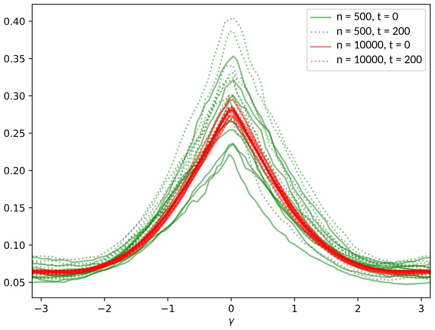
The first experiment illustrates the convergence of the NTK Θ(L)\Theta^{(L)}Θ(L) of a network of depth L=4L=4L=4 for two different widths n=500,10000n=500,10000n=500,10000. The function Θ(4)(x0,x)\Theta^{(4)}(x_{0},x)Θ(4)(x0​,x) is plotted for a fixed x0=(1,0)x_{0}=(1,0)x0​=(1,0) and x=(cos⁡(γ),sin⁡(γ))x=(\cos(\gamma),\sin(\gamma))x=(cos(γ),sin(γ)) on the unit circle in Figure 1. To observe the distribution of the NTK, 10 independent initializations are performed for both widths. The kernels are plotted at initialization t=0t=0t=0 and then after 200 steps of gradient descent with learning rate 1.01.01.0 (i.e. at t=200t=200t=200). We approximate the function f∗(x)=x1x2f^{*}(x)=x_{1}x_{2}f∗(x)=x1​x2​ with a least-squares cost on random N(0,1)\mathcal{N}(0,1)N(0,1) inputs.

第一个实验展示深度 L=4L=4L=4 的网络在两种宽度 n=500,10000n=500,10000n=500,10000 下 NTK Θ(L)\Theta^{(L)}Θ(L) 的收敛。图 1 画出了固定 x0=(1,0)x_{0}=(1,0)x0​=(1,0)、以及单位圆上 x=(cos⁡(γ),sin⁡(γ))x=(\cos(\gamma),\sin(\gamma))x=(cos(γ),sin(γ)) 时的函数 Θ(4)(x0,x)\Theta^{(4)}(x_{0},x)Θ(4)(x0​,x)。为观察 NTK 的分布,两种宽度各做了 10 次独立初始化。核先画在初始化 t=0t=0t=0,再画在学习率为 1.01.01.0 的梯度下降 200 步之后(即 t=200t=200t=200)。我们在随机 N(0,1)\mathcal{N}(0,1)N(0,1) 输入上用最小二乘代价来逼近函数 f∗(x)=x1x2f^{*}(x)=x_{1}x_{2}f∗(x)=x1​x2​。

Convergence of the NTK to a fixed limit

Figure 1: Convergence of the NTK to a fixed limit for two widths nnn and two times ttt.

图 1:两种宽度 nnn、两个时刻 ttt 下,NTK 向固定极限的收敛。

For the wider network, the NTK shows less variance and is smoother. It is interesting to note that the expectation of the NTK is very close for both networks widths. After 200 steps of training, we observe that the NTK tends to “inflate”. As expected, this effect is much less apparent for the wider network (n=10000n=10000n=10000) where the NTK stays almost fixed, than for the smaller network (n=500n=500n=500).

对更宽的网络,NTK 的方差更小,曲线也更光滑。有意思的是,两种宽度下 NTK 的期望非常接近。训练 200 步之后,我们观察到 NTK 往往会“膨胀”。正如所料,这一效应在更宽的网络(n=10000n=10000n=10000,NTK 几乎不动)上远不如在较小的网络(n=500n=500n=500)上明显。

6.2 Kernel regression

6.2 核回归

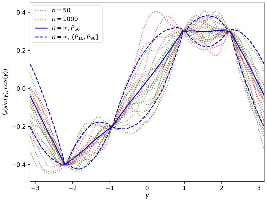
For a regression cost, the infinite-width limit network function fθ(t)f_{\theta}(t)fθ​(t) has a Gaussian distribution for all times ttt and in particular at convergence t→∞t\to\inftyt→∞ (see Section 5). We compared the theoretical Gaussian distribution at t→∞t\to\inftyt→∞ to the distribution of the network function fθ(T)f_{\theta}(T)fθ​(T) of a finite-width network for a large time T=1000T=1000T=1000. For two different widths n=50,1000n=50,1000n=50,1000 and for 10 random initializations each, a network is trained on a least-squares cost on 4 points of the unit circle for 1000 steps with learning rate 1.01.01.0 and then plotted in Figure 2.

对回归代价,无限宽极限下的网络函数 fθ(t)f_{\theta}(t)fθ​(t) 在所有时刻 ttt 都是高斯分布,特别是在收敛 t→∞t\to\inftyt→∞ 时(见第 5 节)。我们把 t→∞t\to\inftyt→∞ 时的理论高斯分布,与有限宽网络在较大时刻 T=1000T=1000T=1000 的网络函数 fθ(T)f_{\theta}(T)fθ​(T) 的分布做了比较。对两种宽度 n=50,1000n=50,1000n=50,1000,各做 10 次随机初始化:网络在单位圆上的 4 个点上、以学习率 1.01.01.0 用最小二乘代价训练 1000 步,然后画在图 2 中。

Network functions near convergence compared with the limiting Gaussian

Figure 2: Networks function fθf_{\theta}fθ​ near convergence for two widths nnn and 10th, 50th and 90th percentiles of the asymptotic Gaussian distribution.

图 2:两种宽度 nnn 下接近收敛的网络函数 fθf_{\theta}fθ​,以及渐近高斯分布的第 10、50、90 百分位。

We also approximated the kernels Θ∞(4)\Theta^{(4)}_{\infty}Θ∞(4)​ and Σ(4)\Sigma^{(4)}Σ(4) using a large-width network (n=10000n=10000n=10000) and used them to calculate and plot the 10th, 50th and 90-th percentiles of the t→∞t\to\inftyt→∞ limiting Gaussian distribution.

我们还用一个大宽度网络(n=10000n=10000n=10000)逼近了核 Θ∞(4)\Theta^{(4)}_{\infty}Θ∞(4)​ 和 Σ(4)\Sigma^{(4)}Σ(4),并用它们计算并画出 t→∞t\to\inftyt→∞ 极限高斯分布的第 10、50 和 90 百分位。

The distributions of the network functions are very similar for both widths: their mean and variance appear to be close to those of the limiting distribution t→∞t\to\inftyt→∞. Even for relatively small widths (n=50n=50n=50), the NTK gives a good indication of the distribution of fθ(t)f_{\theta}(t)fθ​(t) as t→∞t\to\inftyt→∞.

两种宽度下网络函数的分布非常相似:它们的均值和方差看起来都接近 t→∞t\to\inftyt→∞ 的极限分布。即便宽度相对较小(n=50n=50n=50),NTK 也能很好地指示 t→∞t\to\inftyt→∞ 时 fθ(t)f_{\theta}(t)fθ​(t) 的分布。

6.3 Convergence along a principal component

6.3 沿主成分的收敛

We now illustrate our result on the MNIST dataset of handwritten digits made up of grayscale images of dimension 28×2828\times 2828×28, yielding a dimension of n0=784n_{0}=784n0​=784.

现在我们在 MNIST 手写数字数据集上说明我们的结果。这些灰度图像的尺寸是 28×2828\times 2828×28,因而 n0=784n_{0}=784n0​=784。

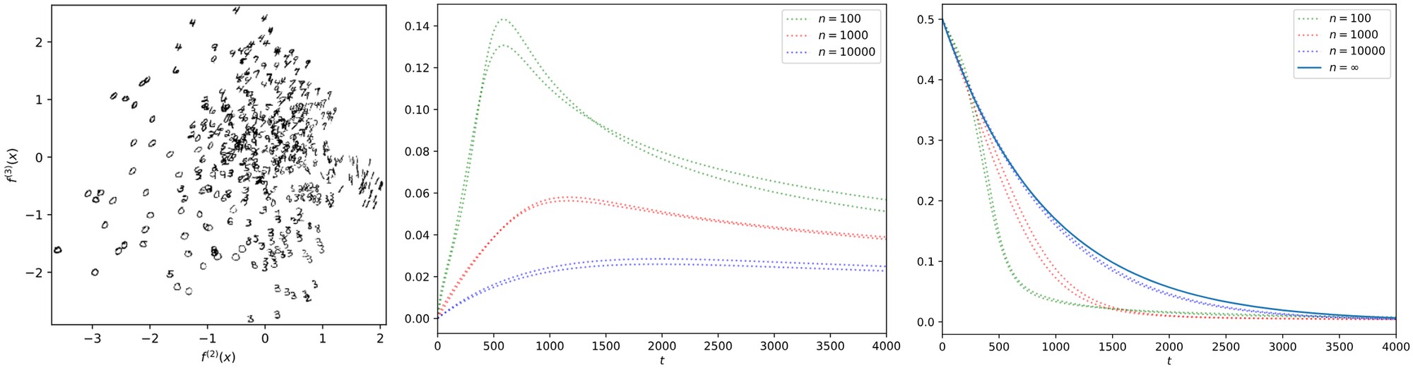
We computed the first 3 principal components of a batch of N=512N=512N=512 digits with respect to the NTK of a high-width network n=10000n=10000n=10000 (giving an approximation of the limiting kernel) using a power iteration method. The respective eigenvalues are λ1=0.0457\lambda_{1}=0.0457λ1​=0.0457, λ2=0.00108\lambda_{2}=0.00108λ2​=0.00108 and λ3=0.00078\lambda_{3}=0.00078λ3​=0.00078. The kernel PCA is non-centered, the first component is therefore almost equal to the constant function, which explains the large gap between the first and second eigenvalues.3^{3}3 The next two components are much more interesting as can be seen in Figure 3a, where the batch is plotted with xxx and yyy coordinates corresponding to the 2nd and 3rd components.

我们对一批 N=512N=512N=512 张数字,用幂迭代法计算了相对于高宽度网络 n=10000n=10000n=10000 的 NTK(作为极限核的逼近)的前 3 个主成分。相应的特征值是 λ1=0.0457\lambda_{1}=0.0457λ1​=0.0457、λ2=0.00108\lambda_{2}=0.00108λ2​=0.00108 和 λ3=0.00078\lambda_{3}=0.00078λ3​=0.00078。这里的核 PCA 是非中心的,因此第一主成分几乎等于常函数,这也解释了第一与第二特征值之间的巨大差距。3^{3}3 后两个成分要有意思得多,如图 3a 所示:该批次被画在以第 2、第 3 主成分为 xxx、yyy 坐标的平面上。

3^{3}3It can be observed numerically, that if we choose β=1.0\beta=1.0β=1.0 instead of our recommended 0.10.10.1, the gap between the first and the second principal component is about ten times bigger, which makes training more difficult.

3^{3}3可以数值上观察到:若取 β=1.0\beta=1.0β=1.0 而不是我们建议的 0.10.10.1,第一与第二主成分之间的差距大约要大十倍,训练也会更困难。

We have seen in Section 5 how the convergence of kernel gradient descent follows the kernel principal components. If the difference at initialization f0−f∗f_{0}-f^{*}f0​−f∗ is equal (or proportional) to one of the principal components f(i)f^{(i)}f(i), then the function will converge along a straight line (in the function space) to f∗f^{*}f∗ at an exponential rate e−λite^{-\lambda_{i}t}e−λi​t.

第 5 节已经说明,核梯度下降的收敛如何沿着核主成分进行。若初始化处的差 f0−f∗f_{0}-f^{*}f0​−f∗ 等于(或正比于)某一个主成分 f(i)f^{(i)}f(i),则函数将在函数空间中沿直线以指数速率 e−λite^{-\lambda_{i}t}e−λi​t 收敛到 f∗f^{*}f∗。

We tested whether ANNs of various widths n=100,1000,10000n=100,1000,10000n=100,1000,10000 behave in a similar manner. We set the goal of the regression cost to f∗=fθ(0)+0.5f(2)f^{*}=f_{\theta}(0)+0.5f^{(2)}f∗=fθ​(0)+0.5f(2) and let the network converge. At each time step ttt, we decomposed the difference fθ(t)−f∗f_{\theta}(t)-f^{*}fθ​(t)−f∗ into a component gtg_{t}gt​ proportional to f(2)f^{(2)}f(2) and another one hth_{t}ht​ orthogonal to f(2)f^{(2)}f(2). In the infinite-width limit, the first component decays exponentially fast ∥gt∥pin=0.5e−λ2t\|g_{t}\|_{p^{\mathrm{in}}}=0.5e^{-\lambda_{2}t}∥gt​∥pin​=0.5e−λ2​t while the second is null (ht=0h_{t}=0ht​=0), as the function converges along a straight line.

我们测试了不同宽度 n=100,1000,10000n=100,1000,10000n=100,1000,10000 的 ANN 是否有类似行为。我们把回归代价的目标设为 f∗=fθ(0)+0.5f(2)f^{*}=f_{\theta}(0)+0.5f^{(2)}f∗=fθ​(0)+0.5f(2),并让网络收敛。在每个时刻 ttt,我们把差 fθ(t)−f∗f_{\theta}(t)-f^{*}fθ​(t)−f∗ 分解成正比于 f(2)f^{(2)}f(2) 的分量 gtg_{t}gt​,以及与 f(2)f^{(2)}f(2) 正交的分量 hth_{t}ht​。在无限宽极限下,第一个分量按指数快速衰减 ∥gt∥pin=0.5e−λ2t\|g_{t}\|_{p^{\mathrm{in}}}=0.5e^{-\lambda_{2}t}∥gt​∥pin​=0.5e−λ2​t,而第二个分量为零(ht=0h_{t}=0ht​=0),因为函数沿直线收敛。

MNIST kernel PCA and convergence along the second principal component

Figure 3. (a) The 2nd and 3rd principal components of MNIST. (b) Deviation of the network function fθf_{\theta}fθ​ from the straight line. (c) Convergence of fθf_{\theta}fθ​ along the 2nd principal component.

图 3.(a)MNIST 的第 2、第 3 主成分。(b)网络函数 fθf_{\theta}fθ​ 相对直线的偏离。(c)fθf_{\theta}fθ​ 沿第 2 主成分的收敛。

As expected, we see in Figure 3b that the wider the network, the less it deviates from the straight line (for each width nnn we performed two independent trials). As the width grows, the trajectory along the 2nd principal component (shown in Figure 3c) converges to the theoretical limit shown in blue.

正如所料,图 3b 显示网络越宽,偏离直线就越少(每种宽度 nnn 我们做了两次独立试验)。随着宽度增大,沿第 2 主成分的轨迹(图 3c)收敛到以蓝色画出的理论极限。

A surprising observation is that smaller networks appear to converge faster than wider ones. This may be explained by the inflation of the NTK observed in our first experiment. Indeed, multiplying the NTK by a factor aaa is equivalent to multiplying the learning rate by the same factor. However, note that since the NTK of large-width network is more stable during training, larger learning rates can in principle be taken. One must hence be careful when comparing the convergence speed in terms of the number of steps (rather than in terms of the time ttt): both the inflation effect and the learning rate must be taken into account.

一个出人意料的观察是:较小的网络看起来比更宽的网络收敛更快。这或许可以由第一个实验中观察到的 NTK 膨胀来解释。的确,把 NTK 乘上一个因子 aaa,等价于把学习率乘上同一个因子。但要注意,由于大宽度网络的 NTK 在训练中更稳定,原则上可以取更大的学习率。因此,在按步数(而不是按时间 ttt)比较收敛速度时必须小心:膨胀效应和学习率都要计算进去。

7 Conclusion

7 结论

This paper introduces a new tool to study ANNs, the Neural Tangent Kernel (NTK), which describes the local dynamics of an ANN during gradient descent. This leads to a new connection between ANN training and kernel methods: in the infinite-width limit, an ANN can be described in the function space directly by the limit of the NTK, an explicit constant kernel Θ∞(L)\Theta^{(L)}_{\infty}Θ∞(L)​, which only depends on its depth, nonlinearity and parameter initialization variance. More precisely, in this limit, ANN gradient descent is shown to be equivalent to a kernel gradient descent with respect to Θ∞(L)\Theta^{(L)}_{\infty}Θ∞(L)​. The limit of the NTK is hence a powerful tool to understand the generalization properties of ANNs, and it allows one to study the influence of the depth and nonlinearity on the learning abilities of the network. The analysis of training using NTK allows one to relate convergence of ANN training with the positive-definiteness of the limiting NTK and leads to a characterization of the directions favored by early stopping methods.

本文引入一个研究 ANN 的新工具——神经正切核(NTK),它描述 ANN 在梯度下降中的局部动力学。这在 ANN 训练与核方法之间建立了新的联系:在无限宽极限下,ANN 可以在函数空间中直接由 NTK 的极限来描述,也就是一个可以显式写出的常数核 Θ∞(L)\Theta^{(L)}_{\infty}Θ∞(L)​,它只依赖于深度、非线性以及参数初始化方差。更精确地说,在这一极限下,ANN 梯度下降被证明等价于相对于 Θ∞(L)\Theta^{(L)}_{\infty}Θ∞(L)​ 的核梯度下降。因此,NTK 的极限是理解 ANN 泛化性质的有力工具,也使人可以研究深度和非线性对网络学习能力的影响。用 NTK 分析训练,可以把 ANN 训练的收敛与极限 NTK 的正定性联系起来,并刻画早停方法所偏爱的方向。

Acknowledgements

致谢

The authors thank K. Kytölä for many interesting discussions. The second author was supported by the ERC CG CRITICAL. The last author acknowledges support from the ERC SG Constamis, the NCCR SwissMAP, the Blavatnik Family Foundation and the Latsis Foundation.

作者感谢 K. Kytölä 的许多有趣讨论。第二作者得到 ERC CG CRITICAL 的资助。末位作者感谢 ERC SG Constamis、NCCR SwissMAP、Blavatnik Family Foundation 和 Latsis Foundation 的支持。

References

参考文献

[1] M. Belkin, S. Ma, and S. Mandal. To understand deep learning we need to understand kernel learning. arXiv preprint, Feb 2018.

[2] Y. Cho and L. K. Saul. Kernel methods for deep learning. In Advances in Neural Information Processing Systems 22, pages 342–350. Curran Associates, Inc., 2009.

[3] A. Choromanska, M. Henaff, M. Mathieu, G. B. Arous, and Y. LeCun. The Loss Surfaces of Multilayer Networks. Journal of Machine Learning Research, 38:192–204, nov 2015.

[4] Y. N. Dauphin, R. Pascanu, C. Gulcehre, K. Cho, S. Ganguli, and Y. Bengio. Identifying and attacking the saddle point problem in high-dimensional non-convex optimization. In Proceedings of the 27th International Conference on Neural Information Processing Systems - Volume 2, NIPS’14, pages 2933–2941, Cambridge, MA, USA, 2014. MIT Press.

[5] S. S. Dragomir. Some Gronwall Type Inequalities and Applications. Nova Science Publishers, 2003.

[6] I. J. Goodfellow, J. Pouget-Abadie, M. Mirza, B. Xu, D. Warde-Farley, S. Ozair, A. Courville, and Y. Bengio. Generative Adversarial Networks. NIPS’14 Proceedings of the 27th International Conference on Neural Information Processing Systems - Volume 2, pages 2672–2680, jun 2014.

[7] K. Hornik, M. Stinchcombe, and H. White. Multilayer feedforward networks are universal approximators. Neural Networks, 2(5):359–366, 1989.

[8] R. Karakida, S. Akaho, and S.-i. Amari. Universal Statistics of Fisher Information in Deep Neural Networks: Mean Field Approach. jun 2018.

[9] J. H. Lee, Y. Bahri, R. Novak, S. S. Schoenholz, J. Pennington, and J. Sohl-Dickstein. Deep neural networks as gaussian processes. ICLR, 2018.

[10] M. Leshno, V. Lin, A. Pinkus, and S. Schocken. Multilayer feedforward networks with a non-polynomial activation function can approximate any function. Neural Networks, 6(6):861–867, 1993.

[11] S. Mei, A. Montanari, and P.-M. Nguyen. A mean field view of the landscape of two-layer neural networks. Proceedings of the National Academy of Sciences, 115(33):E7665–E7671, 2018.

[12] R. M. Neal. Bayesian Learning for Neural Networks. Springer-Verlag New York, Inc., Secaucus, NJ, USA, 1996.

[13] R. Pascanu, Y. N. Dauphin, S. Ganguli, and Y. Bengio. On the saddle point problem for non-convex optimization. arXiv preprint, 2014.

[14] J. Pennington and Y. Bahri. Geometry of neural network loss surfaces via random matrix theory. In Proceedings of the 34th International Conference on Machine Learning, volume 70 of Proceedings of Machine Learning Research, pages 2798–2806, International Convention Centre, Sydney, Australia, 06–11 Aug 2017. PMLR.

[15] A. Rahimi and B. Recht. Random features for large-scale kernel machines. In Advances in Neural Information Processing Systems 20, pages 1177–1184. Curran Associates, Inc., 2008.

[16] L. Sagun, U. Evci, V. U. Güney, Y. Dauphin, and L. Bottou. Empirical analysis of the hessian of over-parametrized neural networks. CoRR, abs/1706.04454, 2017.

[17] B. Schölkopf, A. Smola, and K.-R. Müller. Nonlinear component analysis as a kernel eigenvalue problem. Neural Computation, 10(5):1299–1319, 1998.

[18] J. Shawe-Taylor and N. Cristianini. Kernel Methods for Pattern Analysis. Cambridge University Press, New York, NY, USA, 2004.

[19] C. Zhang, S. Bengio, M. Hardt, B. Recht, and O. Vinyals. Understanding deep learning requires rethinking generalization. ICLR 2017 proceedings, Feb 2017.

The following four references appear in the arXiv v4 appendix (pages 11–19) but are not in the official NeurIPS 2018 10-page bibliography. They are numbered [20]–[23] here; appendix citations have been remapped to this combined list (official [1]–[19] plus these four).

以下四条文献出现在 arXiv v4 附录(第 11–19 页)中,但不在官方 NeurIPS 2018 的 10 页参考文献里。这里编号为 [20]–[23];附录中的引用已映射到这份合并目录(官方 [1]–[19] 加上这四条)。

[20] A. Daniely, R. Frostig, and Y. Singer. Toward deeper understanding of neural networks: The power of initialization and a dual view on expressivity. In D. D. Lee, M. Sugiyama, U. V. Luxburg, I. Guyon, and R. Garnett, editors, Advances in Neural Information Processing Systems 29, pages 2253–2261. Curran Associates, Inc., 2016.

[21] A. G. de G. Matthews, J. Hron, M. Rowland, R. E. Turner, and Z. Ghahramani. Gaussian process behaviour in wide deep neural networks. In International Conference on Learning Representations, 2018.

[22] A. G. de G. Matthews, J. Hron, R. E. Turner, and Z. Ghahramani. Sample-then-optimize posterior sampling for bayesian linear models. In NIPS workshop on Advances in Approximate Bayesian Inference, 2017.

[23] T. Gneiting. Strictly and non-strictly positive definite functions on spheres. Bernoulli, 19(4):1327–1349, 2013.

Appendix A Appendix

附录 A 附录

This appendix is dedicated to proving the key results of this paper, namely Proposition 1 and Theorems 1 and 2, which describe the asymptotics of neural networks at initialization and during training.

本附录用于证明本文的关键结果,即命题 1 以及定理 1 和定理 2,它们描述神经网络在初始化时以及训练过程中的渐近行为。

We study the limit of the NTK as n1,...,nL−1→∞n_{1},...,n_{L-1}\to\inftyn1​,...,nL−1​→∞ sequentially, i.e. we first take n1→∞n_{1}\to\inftyn1​→∞, then n2→∞n_{2}\to\inftyn2​→∞, etc. This leads to much simpler proofs, but our results could in principle be strengthened to the more general setting when min⁡(n1,...,nL−1)→∞\min(n_{1},...,n_{L-1})\to\inftymin(n1​,...,nL−1​)→∞.

我们按顺序研究 NTK 在 n1,…,nL−1→∞n_{1},\ldots,n_{L-1}\to\inftyn1​,…,nL−1​→∞ 时的极限,也就是先取 n1→∞n_{1}\to\inftyn1​→∞,再取 n2→∞n_{2}\to\inftyn2​→∞,以此类推。这使证明简单得多,但我们的结果原则上可以加强到 min⁡(n1,…,nL−1)→∞\min(n_{1},\ldots,n_{L-1})\to\inftymin(n1​,…,nL−1​)→∞ 这一更一般的设定。

A natural choice of convergence to study the NTK is with respect to the operator norm on kernels:

研究 NTK 时,一种自然的收敛选取是相对于核上的算子范数:

∥K∥op=max⁡∥f∥pin≤1∥f∥K=max⁡∥f∥pin≤1Ex,x′[f(x)TK(x,x′)f(x′)],\lVert K\rVert_{op}=\max_{\lVert f\rVert_{p^{in}}\leq 1}\lVert f\rVert_{K}=\max_{\lVert f\rVert_{p^{in}}\leq 1}\sqrt{\mathbb{E}_{x,x^{\prime}}[f(x)^{T}K(x,x^{\prime})f(x^{\prime})]},∥K∥op​=∥f∥pin​≤1max​∥f∥K​=∥f∥pin​≤1max​Ex,x′​[f(x)TK(x,x′)f(x′)]​,

where the expectation is taken over two independent x,x′∼pinx,x^{\prime}\sim p^{in}x,x′∼pin. This norm depends on the input distribution pinp^{in}pin. In our setting, pinp^{in}pin is taken to be the empirical measure of a finite dataset of distinct samples x1,...,xNx_{1},...,x_{N}x1​,...,xN​. As a result, the operator norm of KKK is equal to the leading eigenvalue of the NnL×NnLNn_{L}\times Nn_{L}NnL​×NnL​ Gram matrix (Kkk′(xi,xj))k,k′<nL,i,j<N\left(K_{kk^{\prime}}(x_{i},x_{j})\right)_{k,k^{\prime}<n_{L},i,j<N}(Kkk′​(xi​,xj​))k,k′<nL​,i,j<N​. In our setting, convergence in operator norm is hence equivalent to pointwise convergence of KKK on the dataset.

其中期望对两个独立的 x,x′∼pinx,x'\sim p^{\mathrm{in}}x,x′∼pin 来取。这一范数依赖于输入分布 pinp^{\mathrm{in}}pin。在我们的设定中,pinp^{\mathrm{in}}pin 取为一组互不相同的有限样本 x1,…,xNx_{1},\ldots,x_{N}x1​,…,xN​ 的经验测度。因此,KKK 的算子范数等于 NnL×NnLNn_{L}\times Nn_{L}NnL​×NnL​ 的 Gram 矩阵 (Kkk′(xi,xj))k,k′<nL, i,j<N\bigl(K_{kk'}(x_{i},x_{j})\bigr)_{k,k'<n_{L},\,i,j<N}(Kkk′​(xi​,xj​))k,k′<nL​,i,j<N​ 的最大特征值。于是在我们的设定中,算子范数收敛等价于 KKK 在数据集上的逐点收敛。

A.1 Asymptotics at Initialization

A.1 初始化时的渐近

It has already been observed [12, 9] that the output functions fθ,if_{\theta,i}fθ,i​ for i=1,...,nLi=1,...,n_{L}i=1,...,nL​ tend to iid Gaussian processes in the infinite-width limit.

已经有人观察到 [12, 9],输出函数 fθ,if_{\theta,i}fθ,i​(i=1,…,nLi=1,\ldots,n_{L}i=1,…,nL​)在无限宽极限下趋于独立同分布的高斯过程。

Proposition 1.

For a network of depth LLL at initialization, with a Lipschitz nonlinearity σ\sigmaσ, and in the limit as n1,...,nL−1→∞n_{1},...,n_{L-1}\to\inftyn1​,...,nL−1​→∞ sequentially, the output functions fθ,kf_{\theta,k}fθ,k​, for k=1,...,nLk=1,...,n_{L}k=1,...,nL​, tend (in law) to iid centered Gaussian processes of covariance Σ(L)\Sigma^{(L)}Σ(L), where Σ(L)\Sigma^{(L)}Σ(L) is defined recursively by:

命题 1. 对深度为 LLL、非线性 σ\sigmaσ 为 Lipschitz 的网络,在初始化时,当 n1,…,nL−1→∞n_{1},\ldots,n_{L-1}\to\inftyn1​,…,nL−1​→∞ 按顺序取极限时,输出函数 fθ,kf_{\theta,k}fθ,k​(k=1,…,nLk=1,\ldots,n_{L}k=1,…,nL​)依分布趋于协方差为 Σ(L)\Sigma^{(L)}Σ(L) 的独立同分布中心高斯过程,其中 Σ(L)\Sigma^{(L)}Σ(L) 由下述递归定义:

Σ(1)(x,x′)=1n0xTx′+β2Σ(L+1)(x,x′)=Ef[σ(f(x))σ(f(x′))]+β2,\displaystyle\Sigma^{(1)}(x,x^{\prime}) \\ \displaystyle=\frac{1}{n_{0}}x^{T}x^{\prime}+\beta^{2} \\ \displaystyle\Sigma^{(L+1)}(x,x^{\prime}) \\ \displaystyle=\mathbb{E}_{f}[\sigma(f(x))\sigma(f(x^{\prime}))]+\beta^{2},Σ(1)(x,x′)=n0​1​xTx′+β2Σ(L+1)(x,x′)=Ef​[σ(f(x))σ(f(x′))]+β2,

taking the expectation with respect to a centered Gaussian process fff of covariance Σ(L)\Sigma^{(L)}Σ(L).

期望是对协方差为 Σ(L)\Sigma^{(L)}Σ(L) 的中心高斯过程 fff 来取的。

Proof.

We prove the result by induction. When L=1L=1L=1, there are no hidden layers and fθf_{\theta}fθ​ is a random affine function of the form:

证明.

我们用归纳法证明。当 L=1L=1L=1 时,没有隐层,fθf_{\theta}fθ​ 是如下形式的随机仿射函数:

fθ(x)=1n0W(0)x+βb(0).f_{\theta}(x)=\frac{1}{\sqrt{n_{0}}}W^{(0)}x+\beta b^{(0)}.fθ​(x)=n0​​1​W(0)x+βb(0).

All output functions fθ,kf_{\theta,k}fθ,k​ are hence independent and have covariance Σ(1)\Sigma^{(1)}Σ(1) as needed.

因此所有输出函数 fθ,kf_{\theta,k}fθ,k​ 相互独立,并且具有所需的协方差 Σ(1)\Sigma^{(1)}Σ(1)。

The key to the induction step is to consider an (L+1)(L+1)(L+1)-network as the following composition: an LLL-network Rn0→RnL\mathbb{R}^{n_{0}}\to\mathbb{R}^{n_{L}}Rn0​→RnL​ mapping the input to the pre-activations α~i(L)\tilde{\alpha}^{(L)}_{i}α~i(L)​, followed by an elementwise application of the nonlinearity σ\sigmaσ and then a random affine map RnL→RnL+1\mathbb{R}^{n_{L}}\to\mathbb{R}^{n_{L+1}}RnL​→RnL+1​. The induction hypothesis gives that in the limit as sequentially n1,...,nL−1→∞n_{1},...,n_{L-1}\to\inftyn1​,...,nL−1​→∞ the preactivations α~i(L)\tilde{\alpha}^{(L)}_{i}α~i(L)​ tend to iid Gaussian processes with covariance Σ(L)\Sigma^{(L)}Σ(L). The outputs

归纳步骤的关键,是把一个 (L+1)(L+1)(L+1) 层网络看成如下复合:一个把输入映到预激活 α~i(L)\tilde{\alpha}^{(L)}_{i}α~i(L)​ 的 LLL 层网络 Rn0→RnL\mathbb{R}^{n_{0}}\to\mathbb{R}^{n_{L}}Rn0​→RnL​,再按分量作用非线性 σ\sigmaσ,然后接一个随机仿射映射 RnL→RnL+1\mathbb{R}^{n_{L}}\to\mathbb{R}^{n_{L+1}}RnL​→RnL+1​。归纳假设给出:当 n1,…,nL−1→∞n_{1},\ldots,n_{L-1}\to\inftyn1​,…,nL−1​→∞ 按顺序取极限时,预激活 α~i(L)\tilde{\alpha}^{(L)}_{i}α~i(L)​ 趋于协方差为 Σ(L)\Sigma^{(L)}Σ(L) 的独立同分布高斯过程。输出

fθ,i=1nLWi(L)α(L)+βbi(L)f_{\theta,i}=\frac{1}{\sqrt{n_{L}}}W_{i}^{(L)}\alpha^{(L)}+\beta b_{i}^{(L)}fθ,i​=nL​​1​Wi(L)​α(L)+βbi(L)​

conditioned on the values of α(L)\alpha^{(L)}α(L) are iid centered Gaussians with covariance

在给定 α(L)\alpha^{(L)}α(L) 的条件下,是协方差如下的独立同分布中心高斯:

Σ~(L+1)(x,x′)=1nLα(L)(x;θ)Tα(L)(x′;θ)+β2.\tilde{\Sigma}^{(L+1)}(x,x^{\prime})=\frac{1}{n_{L}}\alpha^{(L)}(x;\theta)^{T}\alpha^{(L)}(x^{\prime};\theta)+\beta^{2}.Σ~(L+1)(x,x′)=nL​1​α(L)(x;θ)Tα(L)(x′;θ)+β2.

By the law of large numbers, as nL→∞n_{L}\to\inftynL​→∞, this covariance tends in probability to the expectation

由大数定律,当 nL→∞n_{L}\to\inftynL​→∞ 时,这一协方差依概率趋于期望

Σ~(L+1)(x,x′)→Σ(L+1)(x,x′)=Ef∼N(0,Σ(L))[σ(f(x))σ(f(x′))]+β2.\tilde{\Sigma}^{(L+1)}(x,x^{\prime})\to\Sigma^{(L+1)}(x,x^{\prime})=\mathbb{E}_{f\sim\mathcal{N}(0,\Sigma^{(L)})}[\sigma(f(x))\sigma(f(x^{\prime}))]+\beta^{2}.Σ~(L+1)(x,x′)→Σ(L+1)(x,x′)=Ef∼N(0,Σ(L))​[σ(f(x))σ(f(x′))]+β2.

In particular the covariance is deterministic and hence independent of α(L)\alpha^{(L)}α(L). As a consequence, the conditioned and unconditioned distributions of fθ,if_{\theta,i}fθ,i​ are equal in the limit: they are iid centered Gaussian of covariance Σ(L+1)\Sigma^{(L+1)}Σ(L+1). ∎

特别地,该协方差是确定的,因而与 α(L)\alpha^{(L)}α(L) 独立。因此,在极限下 fθ,if_{\theta,i}fθ,i​ 的条件分布与无条件分布相等:它们是协方差为 Σ(L+1)\Sigma^{(L+1)}Σ(L+1) 的独立同分布中心高斯。∎

In the infinite-width limit, the neural tangent kernel, which is random at initialization, converges in probability to a deterministic limit.

在无限宽极限下,初始化时随机的神经正切核依概率收敛到一个确定性极限。

Theorem 1.

For a network of depth LLL at initialization, with a Lipschitz nonlinearity σ\sigmaσ, and in the limit as the layers width n1,...,nL−1→∞n_{1},...,n_{L-1}\to\inftyn1​,...,nL−1​→∞ sequentially, the NTK Θ(L)\Theta^{(L)}Θ(L) converges in probability to a deterministic limiting kernel:

定理 1. 对深度为 LLL、非线性 σ\sigmaσ 为 Lipschitz 的网络,在初始化时,当各层宽度 n1,…,nL−1→∞n_{1},\ldots,n_{L-1}\to\inftyn1​,…,nL−1​→∞ 按顺序取极限时,NTK Θ(L)\Theta^{(L)}Θ(L) 依概率收敛到一个确定性的极限核:

Θ(L)→Θ∞(L)⊗IdnL.\Theta^{(L)}\to\Theta^{(L)}_{\infty}\otimes Id_{n_{L}}.Θ(L)→Θ∞(L)​⊗IdnL​​.

The scalar kernel Θ∞(L):Rn0×Rn0→R\Theta^{(L)}_{\infty}:\mathbb{R}^{n_{0}}\times\mathbb{R}^{n_{0}}\to\mathbb{R}Θ∞(L)​:Rn0​×Rn0​→R is defined recursively by

标量核 Θ∞(L):Rn0×Rn0→R\Theta^{(L)}_{\infty}:\mathbb{R}^{n_{0}}\times\mathbb{R}^{n_{0}}\to\mathbb{R}Θ∞(L)​:Rn0​×Rn0​→R 由下述递归定义:

Θ∞(1)(x,x′)=Σ(1)(x,x′)Θ∞(L+1)(x,x′)=Θ∞(L)(x,x′)Σ˙(L+1)(x,x′)+Σ(L+1)(x,x′),\displaystyle\Theta^{(1)}_{\infty}(x,x^{\prime}) \\ \displaystyle=\Sigma^{(1)}(x,x^{\prime}) \\ \displaystyle\Theta^{(L+1)}_{\infty}(x,x^{\prime}) \\ \displaystyle=\Theta^{(L)}_{\infty}(x,x^{\prime})\dot{\Sigma}^{(L+1)}(x,x^{\prime})+\Sigma^{(L+1)}(x,x^{\prime}),Θ∞(1)​(x,x′)=Σ(1)(x,x′)Θ∞(L+1)​(x,x′)=Θ∞(L)​(x,x′)Σ˙(L+1)(x,x′)+Σ(L+1)(x,x′),

where

其中

Σ˙(L+1)(x,x′)=Ef∼N(0,Σ(L))[σ˙(f(x))σ˙(f(x′))],\dot{\Sigma}^{(L+1)}\left(x,x^{\prime}\right)=\mathbb{E}_{f\sim\mathcal{N}\left(0,\Sigma^{\left(L\right)}\right)}\left[\dot{\sigma}\left(f\left(x\right)\right)\dot{\sigma}\left(f\left(x^{\prime}\right)\right)\right],Σ˙(L+1)(x,x′)=Ef∼N(0,Σ(L))​[σ˙(f(x))σ˙(f(x′))],

taking the expectation with respect to a centered Gaussian process fff of covariance Σ(L)\Sigma^{(L)}Σ(L), and where σ˙\dot{\sigma}σ˙ denotes the derivative of σ\sigmaσ.

期望是对协方差为 Σ(L)\Sigma^{(L)}Σ(L) 的中心高斯过程 fff 来取的,而 σ˙\dot{\sigma}σ˙ 表示 σ\sigmaσ 的导数。

Proof.

The proof is again by induction. When L=1L=1L=1, there is no hidden layer and therefore no limit to be taken. The neural tangent kernel is a sum over the entries of W(0)W^{(0)}W(0) and those of b(0)b^{(0)}b(0):

证明.

证明同样用归纳法。当 L=1L=1L=1 时,没有隐层,因而也无需取极限。神经正切核是对 W(0)W^{(0)}W(0) 与 b(0)b^{(0)}b(0) 各分量求和:

Θkk′(x,x′)=1n0∑i=1n0∑j=1n1xixi′δjkδjk′+β2∑j=1n1δjkδjk′=1n0xTx′δkk′+β2δkk′=Σ(1)(x,x′)δkk′.\displaystyle\Theta_{kk^{\prime}}(x,x^{\prime}) \\ \displaystyle=\frac{1}{n_{0}}\sum_{i=1}^{n_{0}}\sum_{j=1}^{n_{1}}x_{i}x^{\prime}_{i}\delta_{jk}\delta_{jk^{\prime}}+\beta^{2}\sum_{j=1}^{n_{1}}\delta_{jk}\delta_{jk^{\prime}} \\ \displaystyle=\frac{1}{n_{0}}x^{T}x^{\prime}\delta_{kk^{\prime}}+\beta^{2}\delta_{kk^{\prime}}=\Sigma^{(1)}(x,x^{\prime})\delta_{kk^{\prime}}.Θkk′​(x,x′)=n0​1​i=1∑n0​​j=1∑n1​​xi​xi′​δjk​δjk′​+β2j=1∑n1​​δjk​δjk′​=n0​1​xTx′δkk′​+β2δkk′​=Σ(1)(x,x′)δkk′​.

Here again, the key to prove the induction step is the observation that a network of depth L+1L+1L+1 is an LLL-network mapping the inputs xxx to the preactivations of the LLL-th layer α~(L)(x)\tilde{\alpha}^{(L)}(x)α~(L)(x) followed by a nonlinearity and a random affine function. For a network of depth L+1L+1L+1, let us therefore split the parameters into the parameters θ~\tilde{\theta}θ~ of the first LLL layers and those of the last layer (W(L),b(L))(W^{(L)},b^{(L)})(W(L),b(L)).

这里,证明归纳步骤的关键同样是:一个深度 L+1L+1L+1 的网络,可以看成把输入 xxx 映到第 LLL 层预激活 α~(L)(x)\tilde{\alpha}^{(L)}(x)α~(L)(x) 的 LLL 层网络,再接上非线性以及一个随机仿射函数。因此,对深度 L+1L+1L+1 的网络,我们把参数分成前 LLL 层的参数 θ~\tilde{\theta}θ~,以及最后一层的参数 (W(L),b(L))(W^{(L)},b^{(L)})(W(L),b(L))。

By Proposition 1 and the induction hypothesis, as n1,...,nL−1→∞n_{1},...,n_{L-1}\to\inftyn1​,...,nL−1​→∞ the pre-activations α~i(L)\tilde{\alpha}^{(L)}_{i}α~i(L)​ are iid centered Gaussian with covariance Σ(L)\Sigma^{(L)}Σ(L) and the neural tangent kernel Θii′(L)(x,x′)\Theta^{(L)}_{ii^{\prime}}(x,x^{\prime})Θii′(L)​(x,x′) of the smaller network converges to a deterministic limit:

由命题 1 和归纳假设,当 n1,…,nL−1→∞n_{1},\ldots,n_{L-1}\to\inftyn1​,…,nL−1​→∞ 时,预激活 α~i(L)\tilde{\alpha}^{(L)}_{i}α~i(L)​ 是协方差为 Σ(L)\Sigma^{(L)}Σ(L) 的独立同分布中心高斯,并且较小组网络的神经正切核 Θii′(L)(x,x′)\Theta^{(L)}_{ii'}(x,x')Θii′(L)​(x,x′) 收敛到一个确定性极限:

(∂θ~α~i(L)(x;θ))T∂θ~α~i′(L)(x′;θ)→Θ∞(L)(x,x′)δii′.\left(\partial_{\tilde{\theta}}\tilde{\alpha}^{(L)}_{i}(x;\theta)\right)^{T}\partial_{\tilde{\theta}}\tilde{\alpha}^{(L)}_{i^{\prime}}(x^{\prime};\theta)\to\Theta^{(L)}_{\infty}(x,x^{\prime})\delta_{ii^{\prime}}.(∂θ~​α~i(L)​(x;θ))T∂θ~​α~i′(L)​(x′;θ)→Θ∞(L)​(x,x′)δii′​.

We can split the neural tangent network into a sum over the parameters θ~\tilde{\theta}θ~ of the first LLL layers and the remaining parameters W(L)W^{(L)}W(L) and b(L)b^{(L)}b(L).

我们可以把 neural tangent network 拆成对前 LLL 层参数 θ~\tilde{\theta}θ~ 的求和,以及对剩余参数 W(L)W^{(L)}W(L) 和 b(L)b^{(L)}b(L) 的求和。

For the first sum let us observe that by the chain rule:

对第一项求和,由链式法则可以看到:

∂θ~pfθ,k(x)=1nL∑i=1nL∂θ~pα~i(L)(x;θ)σ˙(α~i(L)(x;θ))Wik(L).\partial_{\tilde{\theta}_{p}}f_{\theta,k}(x)=\frac{1}{\sqrt{n_{L}}}\sum_{i=1}^{n_{L}}\partial_{\tilde{\theta}_{p}}\tilde{\alpha}^{(L)}_{i}(x;\theta)\dot{\sigma}(\tilde{\alpha}^{(L)}_{i}(x;\theta))W^{(L)}_{ik}.∂θ~p​​fθ,k​(x)=nL​​1​i=1∑nL​​∂θ~p​​α~i(L)​(x;θ)σ˙(α~i(L)​(x;θ))Wik(L)​.

By the induction hypothesis, the contribution of the parameters θ~\tilde{\theta}θ~ to the neural tangent kernel Θkk′(L+1)(x,x′)\Theta^{(L+1)}_{kk^{\prime}}(x,x^{\prime})Θkk′(L+1)​(x,x′) therefore converges as n1,...,nL−1→∞n_{1},...,n_{L-1}\to\inftyn1​,...,nL−1​→∞:

由归纳假设,参数 θ~\tilde{\theta}θ~ 对神经正切核 Θkk′(L+1)(x,x′)\Theta^{(L+1)}_{kk'}(x,x')Θkk′(L+1)​(x,x′) 的贡献因此在 n1,…,nL−1→∞n_{1},\ldots,n_{L-1}\to\inftyn1​,…,nL−1​→∞ 时收敛:

1nL ⁣∑i,i′=1nL ⁣Θii′(L)(x,x′)σ˙ ⁣( ⁣α~i(L)(x;θ) ⁣)σ˙ ⁣( ⁣α~i′(L)(x′;θ) ⁣)Wik(L)Wi′k′(L) ⁣→1nL ⁣∑i=1nL ⁣Θ∞(L)(x,x′)σ˙ ⁣( ⁣α~i(L)(x;θ) ⁣)σ˙ ⁣( ⁣α~i(L)(x′;θ) ⁣)Wik(L)Wik′(L)\displaystyle\frac{1}{n_{L}}\!\sum_{i,i^{\prime}=1}^{n_{L}}\!\Theta^{(L)}_{ii^{\prime}}(x,x^{\prime})\dot{\sigma}\!\left(\!\tilde{\alpha}^{(L)}_{i}(x;\theta)\!\right)\dot{\sigma}\!\left(\!\tilde{\alpha}^{(L)}_{i^{\prime}}(x^{\prime};\theta)\!\right)W^{(L)}_{ik}W^{(L)}_{i^{\prime}k^{\prime}} \\ \displaystyle\!\to\frac{1}{n_{L}}\!\sum_{i=1}^{n_{L}}\!\Theta^{(L)}_{\infty}(x,x^{\prime})\dot{\sigma}\!\left(\!\tilde{\alpha}^{(L)}_{i}(x;\theta)\!\right)\dot{\sigma}\!\left(\!\tilde{\alpha}^{(L)}_{i}(x^{\prime};\theta)\!\right)W^{(L)}_{ik}W^{(L)}_{ik^{\prime}}nL​1​i,i′=1∑nL​​Θii′(L)​(x,x′)σ˙(α~i(L)​(x;θ))σ˙(α~i′(L)​(x′;θ))Wik(L)​Wi′k′(L)​→nL​1​i=1∑nL​​Θ∞(L)​(x,x′)σ˙(α~i(L)​(x;θ))σ˙(α~i(L)​(x′;θ))Wik(L)​Wik′(L)​

By the law of large numbers, as nL→∞n_{L}\to\inftynL​→∞, this tends to its expectation which is equal to

由大数定律,当 nL→∞n_{L}\to\inftynL​→∞ 时,它趋于其期望,等于

Θ∞(L)(x,x′)Σ˙(L+1)(x,x′)δkk′.\Theta^{(L)}_{\infty}(x,x^{\prime})\dot{\Sigma}^{(L+1)}(x,x^{\prime})\delta_{kk^{\prime}}.Θ∞(L)​(x,x′)Σ˙(L+1)(x,x′)δkk′​.

It is then easy to see that the second part of the neural tangent kernel, the sum over W(L)W^{(L)}W(L) and b(L)b^{(L)}b(L) converges to Σ(L+1)δkk′\Sigma^{(L+1)}\delta_{kk^{\prime}}Σ(L+1)δkk′​ as n1,...,nL→∞n_{1},...,n_{L}\to\inftyn1​,...,nL​→∞. ∎

然后不难看到,神经正切核的第二部分,也就是对 W(L)W^{(L)}W(L) 和 b(L)b^{(L)}b(L) 的求和,在 n1,…,nL→∞n_{1},\ldots,n_{L}\to\inftyn1​,…,nL​→∞ 时收敛到 Σ(L+1)δkk′\Sigma^{(L+1)}\delta_{kk'}Σ(L+1)δkk′​。∎

A.2 Asymptotics during Training

A.2 训练中的渐近

Given a training direction t↦dt∈Ft\mapsto d_{t}\in\mathcal{F}t↦dt​∈F, a neural network is trained in the following manner: the parameters θp\theta_{p}θp​ are initialized as iid N(0,1)\mathcal{N}(0,1)N(0,1) and follow the differential equation:

给定训练方向 t↦dt∈Ft\mapsto d_{t}\in\mathcal{F}t↦dt​∈F,神经网络按如下方式训练:参数 θp\theta_{p}θp​ 初始化为独立同分布的 N(0,1)\mathcal{N}(0,1)N(0,1),并服从微分方程:

∂tθp(t)=<∂θpF(L),dt>pin.\partial_{t}\theta_{p}(t)=\left<\partial_{\theta_{p}}F^{(L)},d_{t}\right>_{p^{in}}.∂t​θp​(t)=⟨∂θp​​F(L),dt​⟩pin​.

In this context, in the infinite-width limit, the NTK stays constant during training:

在这一设定下,无限宽极限中 NTK 在训练过程中保持不变:

Theorem 2.

Assume that σ\sigmaσ is a Lipschitz, twice differentiable nonlinearity function, with bounded second derivative. For any TTT such that the integral ∫0T∥dt∥pindt\int_{0}^{T}\|d_{t}\|_{p^{in}}dt∫0T​∥dt​∥pin​dt stays stochastically bounded, as n1,...,nL−1→∞n_{1},...,n_{L-1}\to\inftyn1​,...,nL−1​→∞ sequentially, we have, uniformly for t∈[0,T]t\in[0,T]t∈[0,T],

定理 2. 设 σ\sigmaσ 是 Lipschitz、二阶可微且二阶导数有界的非线性函数。对任意使积分 ∫0T∥dt∥pin dt\int_{0}^{T}\|d_{t}\|_{p^{\mathrm{in}}}\,dt∫0T​∥dt​∥pin​dt 保持随机有界的 TTT,当 n1,…,nL−1→∞n_{1},\ldots,n_{L-1}\to\inftyn1​,…,nL−1​→∞ 按顺序取极限时,我们有:对 t∈[0,T]t\in[0,T]t∈[0,T] 一致地,

Θ(L)(t)→Θ∞(L)⊗IdnL.\Theta^{(L)}(t)\to\Theta^{(L)}_{\infty}\otimes Id_{n_{L}}.Θ(L)(t)→Θ∞(L)​⊗IdnL​​.

As a consequence, in this limit, the dynamics of fθf_{\theta}fθ​ is described by the differential equation

因此,在这一极限下,fθf_{\theta}fθ​ 的动力学由下述微分方程描述:

∂tfθ(t)=ΦΘ∞(L)⊗IdnL(<dt,⋅>pin).\displaystyle\partial_{t}f_{\theta(t)}=\Phi_{\Theta^{(L)}_{\infty}\otimes Id_{n_{L}}}\left(\left<d_{t},\cdot\right>_{p^{in}}\right).∂t​fθ(t)​=ΦΘ∞(L)​⊗IdnL​​​(⟨dt​,⋅⟩pin​).

Proof.

As in the previous theorem, the proof is by induction on the depth of the network. When L=1L=1L=1, the neural tangent kernel does not depend on the parameters, it is therefore constant during training.

证明.

与前一定理一样,证明对网络深度做归纳。当 L=1L=1L=1 时,神经正切核不依赖于参数,因此在训练中是常数。

For the induction step, we again split an L+1L+1L+1 network into a network of depth LLL with parameters θ~\tilde{\theta}θ~ and top layer connection weights W(L)W^{(L)}W(L) and bias b(L)b^{(L)}b(L). The smaller network follows the training direction

对归纳步骤,我们再次把 L+1L+1L+1 层网络拆成参数为 θ~\tilde{\theta}θ~ 的深度 LLL 网络,以及顶层连接权重 W(L)W^{(L)}W(L) 和偏置 b(L)b^{(L)}b(L)。较小组网络沿如下训练方向演化:

dt′=σ˙(α~(L)(t))(1nLW(L)(t))Tdtd^{\prime}_{t}=\dot{\sigma}\left(\tilde{\alpha}^{(L)}(t)\right)\left(\frac{1}{\sqrt{n_{L}}}W^{(L)}(t)\right)^{T}d_{t}dt′​=σ˙(α~(L)(t))(nL​​1​W(L)(t))Tdt​

for i=1,…,nLi=1,\ldots,n_{L}i=1,…,nL​, where the function α~i(L)(t)\tilde{\alpha}^{(L)}_{i}(t)α~i(L)​(t) is defined as α~i(L)(⋅;θ(t))\tilde{\alpha}^{(L)}_{i}(\cdot;\theta(t))α~i(L)​(⋅;θ(t)). We now want to apply the induction hypothesis to the smaller network. For this, we need to show that ∫0T∥dt′∥pindt\int_{0}^{T}\lVert d^{\prime}_{t}\rVert_{p^{in}}\mathrm{d}t∫0T​∥dt′​∥pin​dt is stochastically bounded as n1,…,nL→∞n_{1},\ldots,n_{L}\to\inftyn1​,…,nL​→∞. Since σ\sigmaσ is a ccc-Lipschitz function, we have that

其中 i=1,…,nLi=1,\ldots,n_{L}i=1,…,nL​,而函数 α~i(L)(t)\tilde{\alpha}^{(L)}_{i}(t)α~i(L)​(t) 定义为 α~i(L)(⋅;θ(t))\tilde{\alpha}^{(L)}_{i}(\cdot;\theta(t))α~i(L)​(⋅;θ(t))。我们现在要把归纳假设用到这个较小组网络上。为此,需要证明当 n1,…,nL→∞n_{1},\ldots,n_{L}\to\inftyn1​,…,nL​→∞ 时,∫0T∥dt′∥pin dt\int_{0}^{T}\lVert d'_{t}\rVert_{p^{\mathrm{in}}}\,\mathrm{d}t∫0T​∥dt′​∥pin​dt 是随机有界的。由于 σ\sigmaσ 是 ccc-Lipschitz 函数,我们有

∥dt′∥pin≤c∥1nLW(L)(t)∥op∥dt∥pin.\lVert d^{\prime}_{t}\rVert_{p^{in}}\leq c\lVert\frac{1}{\sqrt{n_{L}}}W^{(L)}(t)\rVert_{op}\lVert d_{t}\rVert_{p^{in}}.∥dt′​∥pin​≤c∥nL​​1​W(L)(t)∥op​∥dt​∥pin​.

To apply the induction hypothesis, we now need to bound ∥1nLW(L)(t)∥op\lVert\frac{1}{\sqrt{n_{L}}}W^{(L)}(t)\rVert_{op}∥nL​​1​W(L)(t)∥op​. For this, we use the following lemma, which is proven in Appendix A.3 below:

要把归纳假设用上去,现在需要给 ∥1nLW(L)(t)∥op\lVert\frac{1}{\sqrt{n_{L}}}W^{(L)}(t)\rVert_{\mathrm{op}}∥nL​​1​W(L)(t)∥op​ 一个界。为此我们使用下述引理,其证明见下面的附录 A.3:

Lemma 1.

With the setting of Theorem 2, for a network of depth L+1L+1L+1, for any ℓ=1,…,L\ell=1,\ldots,Lℓ=1,…,L, we have the convergence in probability:

引理 1. 在定理 2 的设定下,对深度为 L+1L+1L+1 的网络,对任意 ℓ=1,…,L\ell=1,\ldots,Lℓ=1,…,L,我们有依概率收敛:

lim⁡nL→∞⋯lim⁡n1→∞sup⁡t∈[0,T]∥1nℓ(W(ℓ)(t)−W(ℓ)(0))∥op=0\lim_{n_{L}\to\infty}\cdots\lim_{n_{1}\to\infty}\sup_{t\in[0,T]}\lVert\frac{1}{\sqrt{n_{\ell}}}\left(W^{(\ell)}(t)-W^{(\ell)}(0)\right)\rVert_{op}=0nL​→∞lim​⋯n1​→∞lim​t∈[0,T]sup​∥nℓ​​1​(W(ℓ)(t)−W(ℓ)(0))∥op​=0

From this lemma, to bound ∥1nLW(L)(t)∥op\lVert\frac{1}{\sqrt{n_{L}}}W^{(L)}(t)\rVert_{op}∥nL​​1​W(L)(t)∥op​, it is hence enough to bound ∥1nLW(L)(0)∥op\lVert\frac{1}{\sqrt{n_{L}}}W^{(L)}(0)\rVert_{op}∥nL​​1​W(L)(0)∥op​. From the law of large numbers, we obtain that the norm of each of the nL+1n_{L+1}nL+1​ rows of W(L)(0)W^{(L)}(0)W(L)(0) is bounded, and hence that ∥1nLW(L)(0)∥op\lVert\frac{1}{\sqrt{n_{L}}}W^{(L)}(0)\rVert_{op}∥nL​​1​W(L)(0)∥op​ is bounded (keep in mind that nL+1n_{L+1}nL+1​ is fixed, while n1,…,nLn_{1},\ldots,n_{L}n1​,…,nL​ grow).

由这一引理,要给 ∥1nLW(L)(t)∥op\lVert\frac{1}{\sqrt{n_{L}}}W^{(L)}(t)\rVert_{\mathrm{op}}∥nL​​1​W(L)(t)∥op​ 一个界,只需给 ∥1nLW(L)(0)∥op\lVert\frac{1}{\sqrt{n_{L}}}W^{(L)}(0)\rVert_{\mathrm{op}}∥nL​​1​W(L)(0)∥op​ 一个界。由大数定律,W(L)(0)W^{(L)}(0)W(L)(0) 的 nL+1n_{L+1}nL+1​ 行中每一行的范数都有界,因而 ∥1nLW(L)(0)∥op\lVert\frac{1}{\sqrt{n_{L}}}W^{(L)}(0)\rVert_{\mathrm{op}}∥nL​​1​W(L)(0)∥op​ 有界(请记住 nL+1n_{L+1}nL+1​ 是固定的,而 n1,…,nLn_{1},\ldots,n_{L}n1​,…,nL​ 在增大)。

From the above considerations, we can apply the induction hypothesis to the smaller network, yielding, in the limit as n1,…,nL→∞n_{1},\ldots,n_{L}\to\inftyn1​,…,nL​→∞ (sequentially), that the dynamics is governed by the constant kernel Θ∞(L)\Theta^{(L)}_{\infty}Θ∞(L)​:

基于以上讨论,我们可以把归纳假设用到较小组网络上,从而在 n1,…,nL→∞n_{1},\ldots,n_{L}\to\inftyn1​,…,nL​→∞(按顺序)的极限下,动力学由常数核 Θ∞(L)\Theta^{(L)}_{\infty}Θ∞(L)​ 支配:

∂tα~i(L)(t)=1nLΦΘ∞(L)(<σ˙(α~i(L)(t))(Wi(L)(t))Tdt,⋅>pin).\partial_{t}\tilde{\alpha}^{(L)}_{i}(t)=\frac{1}{\sqrt{n_{L}}}\Phi_{\Theta^{(L)}_{\infty}}\left(\left<\dot{\sigma}\left(\tilde{\alpha}^{(L)}_{i}(t)\right)\left(W^{(L)}_{i}(t)\right)^{T}d_{t},\cdot\right>_{p^{in}}\right).∂t​α~i(L)​(t)=nL​​1​ΦΘ∞(L)​​(⟨σ˙(α~i(L)​(t))(Wi(L)​(t))Tdt​,⋅⟩pin​).

At the same time, the parameters of the last layer evolve according to

与此同时,最后一层的参数按如下方式演化:

∂tWij(L)(t)=1nL<αi(L)(t),dt,j>pin.\displaystyle\partial_{t}W^{(L)}_{ij}(t) \\ \displaystyle=\frac{1}{\sqrt{n_{L}}}\left<\alpha^{(L)}_{i}(t),d_{t,j}\right>_{p^{in}}.∂t​Wij(L)​(t)=nL​​1​⟨αi(L)​(t),dt,j​⟩pin​.

We want to give an upper bound on the variation of the weights columns Wi(L)(t)W_{i}^{(L)}(t)Wi(L)​(t) and of the activations α~i(L)(t)\tilde{\alpha}^{(L)}_{i}(t)α~i(L)​(t) during training in terms of L2L^{2}L2-norm and pinp^{in}pin-norm respectively. Applying the Cauchy-Schwarz inequality for each jjj, summing and using ∂t∣∣⋅∣∣≤∣∣∂t⋅∣∣\partial_{t}||\cdot||\leq||\partial_{t}\cdot||∂t​∣∣⋅∣∣≤∣∣∂t​⋅∣∣), we have

我们希望分别用 L2L^{2}L2 范数和 pinp^{\mathrm{in}}pin-范数,给权重列 Wi(L)(t)W^{(L)}_{i}(t)Wi(L)​(t) 以及激活 α~i(L)(t)\tilde{\alpha}^{(L)}_{i}(t)α~i(L)​(t) 在训练中的变化一个上界。对每个 jjj 使用柯西–施瓦茨不等式,再求和,并利用 ∂t∥⋅∥≤∥∂t⋅∥\partial_{t}\|\cdot\|\leq\|\partial_{t}\cdot\|∂t​∥⋅∥≤∥∂t​⋅∥,我们得到

∂t∥Wi(L)(t)−Wi(L)(0)∥2≤1nL∣∣αi(L)(t)∣∣pin∣∣dt∣∣pin.\displaystyle\partial_{t}\left\lVert W^{(L)}_{i}(t)-W^{(L)}_{i}(0)\right\rVert_{2} \\ \displaystyle\leq\frac{1}{\sqrt{n_{L}}}||\alpha^{(L)}_{i}(t)||_{p^{in}}||d_{t}||_{p^{in}}.∂t​​Wi(L)​(t)−Wi(L)​(0)​2​≤nL​​1​∣∣αi(L)​(t)∣∣pin​∣∣dt​∣∣pin​.

Now, observing that the operator norm of ΦΘ∞(L)\Phi_{\Theta_{\infty}^{(L)}}ΦΘ∞(L)​​ is equal to ∣∣Θ∞(L)∣∣op||\Theta_{\infty}^{(L)}||_{op}∣∣Θ∞(L)​∣∣op​, defined in the introduction of Appendix A, and using the Cauchy-Schwarz inequality, we get

现在注意到 ΦΘ∞(L)\Phi_{\Theta^{(L)}_{\infty}}ΦΘ∞(L)​​ 的算子范数等于附录 A 引言中定义的 ∥Θ∞(L)∥op\|\Theta^{(L)}_{\infty}\|_{\mathrm{op}}∥Θ∞(L)​∥op​,再使用柯西–施瓦茨不等式,得到

∂t∥α~i(L)(t)−α~i(L)(0)∥pin≤1nL∥Θ∞(L)∥op∥σ˙(α~i(L)(t))∥∞∥Wi(L)(t)∥2∥dt∥pin,\displaystyle\partial_{t}\left\lVert\tilde{\alpha}^{(L)}_{i}(t)-\tilde{\alpha}^{(L)}_{i}(0)\right\rVert_{p^{in}} \\ \displaystyle\leq\frac{1}{\sqrt{n_{L}}}\left\lVert\Theta^{(L)}_{\infty}\right\rVert_{op}\left\lVert\dot{\sigma}\left(\tilde{\alpha}^{(L)}_{i}(t)\right)\right\rVert_{\infty}\left\lVert W^{(L)}_{i}(t)\right\rVert_{2}\left\lVert d_{t}\right\rVert_{p^{in}},∂t​​α~i(L)​(t)−α~i(L)​(0)​pin​≤nL​​1​​Θ∞(L)​​op​​σ˙(α~i(L)​(t))​∞​​Wi(L)​(t)​2​∥dt​∥pin​,

where the sup norm ∥⋅∥∞\lVert\cdot\rVert_{\infty}∥⋅∥∞​ is defined by ∥f∥∞=sup⁡x∣f(x)∣.\left\lVert f\right\lVert_{\infty}=\sup_{x}|f(x)|.∥f∥∞​=supx​∣f(x)∣.

其中上确界范数 ∥⋅∥∞\lVert\cdot\rVert_{\infty}∥⋅∥∞​ 定义为 ∥f∥∞=sup⁡x∣f(x)∣\lVert f\rVert_{\infty}=\sup_{x}|f(x)|∥f∥∞​=supx​∣f(x)∣。

To bound both quantities simultaneously, study the derivative of the quantity

为同时给这两个量一个界,我们考察下述量的导数:

A(t)=∣∣αi(L)(0)∣∣pin+c∥α~i(L)(t)−α~i(L)(0)∥pin+∣∣Wi(L)(0)∣∣2+∥Wi(L)(t)−Wi(L)(0)∥2.A(t)=||\alpha^{(L)}_{i}(0)||_{p^{in}}+c\left\lVert\tilde{\alpha}^{(L)}_{i}(t)-\tilde{\alpha}^{(L)}_{i}(0)\right\rVert_{p^{in}}+||W^{(L)}_{i}(0)||_{2}+\left\lVert W^{(L)}_{i}(t)-W^{(L)}_{i}(0)\right\rVert_{2}.A(t)=∣∣αi(L)​(0)∣∣pin​+c​α~i(L)​(t)−α~i(L)​(0)​pin​+∣∣Wi(L)​(0)∣∣2​+​Wi(L)​(t)−Wi(L)​(0)​2​.

We have

我们有

∂tA(t)≤1nL(c2∥Θ∞(L)∥op∥Wi(L)(t)∥2+∣∣αi(L)(t)∣∣pin)∣∣dt∣∣pin≤max⁡{c2∥Θ∞(L)∥op,1}nL∥dt∥pinA(t),\displaystyle\partial_{t}A(t) \\ \displaystyle\leq\frac{1}{\sqrt{n_{L}}}\left(c^{2}\left\lVert\Theta^{(L)}_{\infty}\right\rVert_{op}\left\lVert W^{(L)}_{i}(t)\right\rVert_{2}+||\alpha^{(L)}_{i}(t)||_{p^{in}}\right)||d_{t}||_{p^{in}} \\ \displaystyle\leq\frac{\max\{c^{2}\|\Theta^{(L)}_{\infty}\|_{op},1\}}{\sqrt{n_{L}}}\|d_{t}\|_{p^{in}}A(t),∂t​A(t)≤nL​​1​(c2​Θ∞(L)​​op​​Wi(L)​(t)​2​+∣∣αi(L)​(t)∣∣pin​)∣∣dt​∣∣pin​≤nL​​max{c2∥Θ∞(L)​∥op​,1}​∥dt​∥pin​A(t),

where, in the first inequality, we have used that ∣σ˙∣≤c|\dot{\sigma}|\leq c∣σ˙∣≤c and, in the second inequality, that the sum ∥Wi(L)(t)∥2+∣∣αi(L)(t)∣∣pin\lVert W^{(L)}_{i}(t)\rVert_{2}+||\alpha^{(L)}_{i}(t)||_{p^{in}}∥Wi(L)​(t)∥2​+∣∣αi(L)​(t)∣∣pin​ is bounded by A(t)A(t)A(t). Applying Grönwall’s Lemma, we now get

其中,第一个不等式用了 ∣σ˙∣≤c|\dot{\sigma}|\leq c∣σ˙∣≤c,第二个不等式用了和 ∥Wi(L)(t)∥2+∥αi(L)(t)∥pin\lVert W^{(L)}_{i}(t)\rVert_{2}+\|\alpha^{(L)}_{i}(t)\|_{p^{\mathrm{in}}}∥Wi(L)​(t)∥2​+∥αi(L)​(t)∥pin​ 被 A(t)A(t)A(t) 控制。再应用 Grönwall 引理,我们得到

A(t)≤A(0)exp⁡(max⁡{c2∥Θ∞(L)∥op,1}nL∫0t∥ds∥pinds).A(t)\leq A(0)\exp\left(\frac{\max\{c^{2}\|\Theta^{(L)}_{\infty}\|_{op},1\}}{\sqrt{n_{L}}}\int_{0}^{t}\|d_{s}\|_{p^{in}}ds\right).A(t)≤A(0)exp(nL​​max{c2∥Θ∞(L)​∥op​,1}​∫0t​∥ds​∥pin​ds).

Note that ∥Θ∞(L)∥op\|\Theta^{(L)}_{\infty}\|_{op}∥Θ∞(L)​∥op​ is constant during training. Clearly the value inside of the exponential converges to zero in probability as nL→∞n_{L}\to\inftynL​→∞ given that the integral ∫0t∥dt∥pinds\int_{0}^{t}\|d_{t}\|_{p^{in}}ds∫0t​∥dt​∥pin​ds stays stochastically bounded. The variations of the activations ∥α~i(L)(t)−α~i(L)(0)∥pin\left\lVert\tilde{\alpha}^{(L)}_{i}(t)-\tilde{\alpha}^{(L)}_{i}(0)\right\rVert_{p^{in}}​α~i(L)​(t)−α~i(L)​(0)​pin​ and weights ∥Wi(L)(t)−Wi(L)(0)∥2\left\lVert W^{(L)}_{i}(t)-W^{(L)}_{i}(0)\right\rVert_{2}​Wi(L)​(t)−Wi(L)​(0)​2​ are bounded by c−1(A(t)−A(0))c^{-1}(A(t)-A(0))c−1(A(t)−A(0)) and A(t)−A(0)A(t)-A(0)A(t)−A(0) respectively, which converge to zero at rate O(1nL)O\left(\frac{1}{\sqrt{n_{L}}}\right)O(nL​​1​).

注意 ∥Θ∞(L)∥op\|\Theta^{(L)}_{\infty}\|_{\mathrm{op}}∥Θ∞(L)​∥op​ 在训练中是常数。显然,只要积分 ∫0t∥ds∥pin ds\int_{0}^{t}\|d_{s}\|_{p^{\mathrm{in}}}\,ds∫0t​∥ds​∥pin​ds 保持随机有界,指数里面的量在 nL→∞n_{L}\to\inftynL​→∞ 时依概率趋于零。激活的变化 ∥α~i(L)(t)−α~i(L)(0)∥pin\bigl\lVert\tilde{\alpha}^{(L)}_{i}(t)-\tilde{\alpha}^{(L)}_{i}(0)\bigr\rVert_{p^{\mathrm{in}}}​α~i(L)​(t)−α~i(L)​(0)​pin​ 以及权重的变化 ∥Wi(L)(t)−Wi(L)(0)∥2\bigl\lVert W^{(L)}_{i}(t)-W^{(L)}_{i}(0)\bigr\rVert_{2}​Wi(L)​(t)−Wi(L)​(0)​2​ 分别被 c−1(A(t)−A(0))c^{-1}(A(t)-A(0))c−1(A(t)−A(0)) 和 A(t)−A(0)A(t)-A(0)A(t)−A(0) 控制,它们以 O(1nL)O\bigl(\frac{1}{\sqrt{n_{L}}}\bigr)O(nL​​1​) 的速率趋于零。

We can now use these bounds to control the variation of the NTK and to prove the theorem. To understand how the NTK evolves, we study the evolution of the derivatives with respect to the parameters. The derivatives with respect to the bias parameters of the top layer ∂bj(L)fθ,j′\partial_{b^{(L)}_{j}}f_{\theta,j^{\prime}}∂bj(L)​​fθ,j′​ are always equal to δjj′\delta_{jj^{\prime}}δjj′​. The derivatives with respect to the connection weights of the top layer are given by

现在我们可以用这些界来控制 NTK 的变化,并证明定理。为理解 NTK 如何演化,我们研究对各参数的导数的演化。对顶层偏置参数的导数 ∂bj(L)fθ,j′\partial_{b^{(L)}_{j}}f_{\theta,j'}∂bj(L)​​fθ,j′​ 始终等于 δjj′\delta_{jj'}δjj′​。对顶层连接权重的导数由下式给出:

∂Wij(L)fθ,j′(x)=1nLαi(L)(x;θ)δjj′.\partial_{W^{(L)}_{ij}}f_{\theta,j^{\prime}}(x)=\frac{1}{\sqrt{n_{L}}}\alpha^{(L)}_{i}(x;\theta)\delta_{jj^{\prime}}.∂Wij(L)​​fθ,j′​(x)=nL​​1​αi(L)​(x;θ)δjj′​.

The pre-activations α~i(L)\tilde{\alpha}^{(L)}_{i}α~i(L)​ evolve at a rate of 1nL\frac{1}{\sqrt{n_{L}}}nL​​1​ and so do the activations αi(L)\alpha^{(L)}_{i}αi(L)​. The summands ∂Wij(L)fθ,j′(x)⊗∂Wij(L)fθ,j′′(x′)\partial_{W^{(L)}_{ij}}f_{\theta,j^{\prime}}(x)\otimes\partial_{W^{(L)}_{ij}}f_{\theta,j^{\prime\prime}}(x^{\prime})∂Wij(L)​​fθ,j′​(x)⊗∂Wij(L)​​fθ,j′′​(x′) of the NTK hence vary at rate of nL−3/2n_{L}^{-3/2}nL−3/2​ which induces a variation of the NTK of rate 1nL\frac{1}{\sqrt{n_{L}}}nL​​1​.

预激活 α~i(L)\tilde{\alpha}^{(L)}_{i}α~i(L)​ 以 1nL\frac{1}{\sqrt{n_{L}}}nL​​1​ 的速率演化,激活 αi(L)\alpha^{(L)}_{i}αi(L)​ 也是如此。因此 NTK 中的求和项 ∂Wij(L)fθ,j′(x)⊗∂Wij(L)fθ,j′′(x′)\partial_{W^{(L)}_{ij}}f_{\theta,j'}(x)\otimes\partial_{W^{(L)}_{ij}}f_{\theta,j''}(x')∂Wij(L)​​fθ,j′​(x)⊗∂Wij(L)​​fθ,j′′​(x′) 以 nL−3/2n_{L}^{-3/2}nL−3/2​ 的速率变化,从而使 NTK 以 1nL\frac{1}{\sqrt{n_{L}}}nL​​1​ 的速率变化。

Finally let us study the derivatives with respect to the parameters of the lower layers

最后我们研究对较低层参数的导数

∂θ~kfθ,j(x)=1nL∑i=1nL∂θ~kα~i(L)(x;θ)σ˙(α~i(L)(x;θ))Wij(L).\partial_{\tilde{\theta}_{k}}f_{\theta,j}(x)=\frac{1}{\sqrt{n_{L}}}\sum_{i=1}^{n_{L}}\partial_{\tilde{\theta}_{k}}\tilde{\alpha}^{(L)}_{i}(x;\theta)\dot{\sigma}\left(\tilde{\alpha}^{(L)}_{i}(x;\theta)\right)W^{(L)}_{ij}.∂θ~k​​fθ,j​(x)=nL​​1​i=1∑nL​​∂θ~k​​α~i(L)​(x;θ)σ˙(α~i(L)​(x;θ))Wij(L)​.

Their contribution to the NTK Θjj′(L+1)(x,x′)\Theta^{(L+1)}_{jj^{\prime}}(x,x^{\prime})Θjj′(L+1)​(x,x′) is

它们对 NTK Θjj′(L+1)(x,x′)\Theta^{(L+1)}_{jj'}(x,x')Θjj′(L+1)​(x,x′) 的贡献是

1nL ⁣∑i,i′=1nL ⁣Θii′(L)(x,x′)σ˙ ⁣( ⁣α~i(L)(x;θ) ⁣)σ˙ ⁣( ⁣α~i′(L)(x′;θ) ⁣)Wij(L)Wi′j′(L).\displaystyle\frac{1}{n_{L}}\!\sum_{i,i^{\prime}=1}^{n_{L}}\!\Theta^{(L)}_{ii^{\prime}}(x,x^{\prime})\dot{\sigma}\!\left(\!\tilde{\alpha}^{(L)}_{i}(x;\theta)\!\right)\dot{\sigma}\!\left(\!\tilde{\alpha}^{(L)}_{i^{\prime}}(x^{\prime};\theta)\!\right)W^{(L)}_{ij}W^{(L)}_{i^{\prime}j^{\prime}}.nL​1​i,i′=1∑nL​​Θii′(L)​(x,x′)σ˙(α~i(L)​(x;θ))σ˙(α~i′(L)​(x′;θ))Wij(L)​Wi′j′(L)​.

By the induction hypothesis, the NTK of the smaller network Θ(L)\Theta^{(L)}Θ(L) tends to Θ∞(L)δii′\Theta^{(L)}_{\infty}\delta_{ii^{\prime}}Θ∞(L)​δii′​ as n1,...,nL−1→∞n_{1},...,n_{L-1}\to\inftyn1​,...,nL−1​→∞. The contribution therefore becomes

由归纳假设,当 n1,…,nL−1→∞n_{1},\ldots,n_{L-1}\to\inftyn1​,…,nL−1​→∞ 时,较小组网络的 NTK Θ(L)\Theta^{(L)}Θ(L) 趋于 Θ∞(L)δii′\Theta^{(L)}_{\infty}\delta_{ii'}Θ∞(L)​δii′​。因此这一贡献变为

1nL ⁣∑i=1nL ⁣Θ∞(L)(x,x′)σ˙ ⁣( ⁣α~i(L)(x;θ) ⁣)σ˙ ⁣( ⁣α~i(L)(x′;θ) ⁣)Wij(L)Wij′(L).\displaystyle\frac{1}{n_{L}}\!\sum_{i=1}^{n_{L}}\!\Theta^{(L)}_{\infty}(x,x^{\prime})\dot{\sigma}\!\left(\!\tilde{\alpha}^{(L)}_{i}(x;\theta)\!\right)\dot{\sigma}\!\left(\!\tilde{\alpha}^{(L)}_{i}(x^{\prime};\theta)\!\right)W^{(L)}_{ij}W^{(L)}_{ij^{\prime}}.nL​1​i=1∑nL​​Θ∞(L)​(x,x′)σ˙(α~i(L)​(x;θ))σ˙(α~i(L)​(x′;θ))Wij(L)​Wij′(L)​.

The connection weights Wij(L)W^{(L)}_{ij}Wij(L)​ vary at rate 1nL\frac{1}{\sqrt{n_{L}}}nL​​1​, inducing a change of the same rate to the whole sum. We simply have to prove that the values σ˙(α~i(L)(x;θ))\dot{\sigma}(\tilde{\alpha}^{(L)}_{i}(x;\theta))σ˙(α~i(L)​(x;θ)) also change at rate 1nL\frac{1}{\sqrt{n_{L}}}nL​​1​. Since the second derivative of σ\sigmaσ is bounded, we have that

连接权重 Wij(L)W^{(L)}_{ij}Wij(L)​ 以 1nL\frac{1}{\sqrt{n_{L}}}nL​​1​ 的速率变化,从而使整个和以同样的速率变化。我们只需再证明 σ˙(α~i(L)(x;θ))\dot{\sigma}(\tilde{\alpha}^{(L)}_{i}(x;\theta))σ˙(α~i(L)​(x;θ)) 的取值也以 1nL\frac{1}{\sqrt{n_{L}}}nL​​1​ 的速率变化。由于 σ\sigmaσ 的二阶导数有界,我们有

∂t(σ˙(α~i(L)(x;θ(t))))=O(∂tα~i(L)(x;θ(t))).\partial_{t}\left(\dot{\sigma}\left(\tilde{\alpha}^{(L)}_{i}(x;\theta(t))\right)\right)=O\left(\partial_{t}\tilde{\alpha}^{(L)}_{i}(x;\theta(t))\right).∂t​(σ˙(α~i(L)​(x;θ(t))))=O(∂t​α~i(L)​(x;θ(t))).

Since ∂tα~i(L)(x;θ(t))\partial_{t}\tilde{\alpha}^{(L)}_{i}(x;\theta(t))∂t​α~i(L)​(x;θ(t)) goes to zero at a rate 1nL\frac{1}{\sqrt{n_{L}}}nL​​1​ by the bound on A(t)A(t)A(t) above, this concludes the proof.

由于由上面 A(t)A(t)A(t) 的界可知 ∂tα~i(L)(x;θ(t))\partial_{t}\tilde{\alpha}^{(L)}_{i}(x;\theta(t))∂t​α~i(L)​(x;θ(t)) 以 1nL\frac{1}{\sqrt{n_{L}}}nL​​1​ 的速率趋于零,证明至此结束。

∎

It is somewhat counterintuitive that the variation of the activations of the hidden layers αi(ℓ)\alpha^{(\ell)}_{i}αi(ℓ)​ during training goes to zero as the width becomes large4^{4}4. It is generally assumed that the purpose of the activations of the hidden layers is to learn “good” representations of the data during training. However note that even though the variation of each individual activation shrinks, the number of neurons grows, resulting in a significant collective effect. This explains why the training of the parameters of each layer ℓ\ellℓ has an influence on the network function fθf_{\theta}fθ​ even though it has asymptotically no influence on the individual activations of the layers ℓ′\ell^{\prime}ℓ′ for ℓ<ℓ′<L\ell<\ell^{\prime}<Lℓ<ℓ′<L.

隐层激活 αi(ℓ)\alpha^{(\ell)}_{i}αi(ℓ)​ 在训练中的变化会随着宽度变大而趋于零,这一点多少有些反直觉。4^{4}4 人们通常假定,隐层激活的作用是在训练中学到数据的“好”表示。但要注意,尽管每个单独激活的变化在缩小,神经元的数目却在增大,从而产生显著的集体效应。这就解释了为什么第 ℓ\ellℓ 层参数的训练仍会影响网络函数 fθf_{\theta}fθ​,即使它在渐近意义上对满足 ℓ<ℓ′<L\ell<\ell'<Lℓ<ℓ′<L 的各层 ℓ′\ell'ℓ′ 的单个激活没有影响。

4^{4}4As a consequence, the pre-activations stay Gaussian during training as well, with the same covariance Σ(ℓ)\Sigma^{(\ell)}Σ(ℓ).

4^{4}4因此,预激活在训练中也保持为高斯,并且具有相同的协方差 Σ(ℓ)\Sigma^{(\ell)}Σ(ℓ)。

A.3 A Priori Control during Training

A.3 训练中的先验控制

The goal of this section is to prove Lemma 1, which is a key ingredient in the proof of Theorem 2. Let us first recall it:

本节的目标是证明引理 1,它是定理 2 证明中的关键步骤。我们先把它复述如下:

Lemma 1.

With the setting of Theorem 2, for a network of depth L+1L+1L+1, for any ℓ=1,…,L\ell=1,\ldots,Lℓ=1,…,L, we have the convergence in probability:

引理 1. 在定理 2 的设定下,对深度为 L+1L+1L+1 的网络,对任意 ℓ=1,…,L\ell=1,\ldots,Lℓ=1,…,L,我们有依概率收敛:

lim⁡nL→∞⋯lim⁡n1→∞sup⁡t∈[0,T]∥1nℓ(W(ℓ)(t)−W(ℓ)(0))∥op=0\lim_{n_{L}\to\infty}\cdots\lim_{n_{1}\to\infty}\sup_{t\in[0,T]}\lVert\frac{1}{\sqrt{n_{\ell}}}\left(W^{(\ell)}(t)-W^{(\ell)}(0)\right)\rVert_{op}=0nL​→∞lim​⋯n1​→∞lim​t∈[0,T]sup​∥nℓ​​1​(W(ℓ)(t)−W(ℓ)(0))∥op​=0

Proof.

We prove the lemma for all ℓ=1,…,L\ell=1,\ldots,Lℓ=1,…,L simultaneously, by expressing the variation of the weights 1nℓW(ℓ)\frac{1}{\sqrt{n_{\ell}}}W^{(\ell)}nℓ​​1​W(ℓ) and activations 1nℓα~(ℓ)\frac{1}{\sqrt{n_{\ell}}}\tilde{\alpha}^{(\ell)}nℓ​​1​α~(ℓ) in terms of ‘back-propagated’ training directions d(1),…,d(L)d^{(1)},\ldots,d^{(L)}d(1),…,d(L) associated with the lower layers and the NTKs of the corresponding subnetworks:

证明.

我们对所有 ℓ=1,…,L\ell=1,\ldots,Lℓ=1,…,L 同时证明该引理:把权重 1nℓW(ℓ)\frac{1}{\sqrt{n_{\ell}}}W^{(\ell)}nℓ​​1​W(ℓ) 和激活 1nℓα~(ℓ)\frac{1}{\sqrt{n_{\ell}}}\tilde{\alpha}^{(\ell)}nℓ​​1​α~(ℓ) 的变化,用与较低层相联系的“反向传播”训练方向 d(1),…,d(L)d^{(1)},\ldots,d^{(L)}d(1),…,d(L) 以及相应子网络的 NTK 来表达:

  1. At all times, the evolution of the preactivations and weights is given by: ∂tα~(ℓ)\displaystyle\partial_{t}\tilde{\alpha}^{(\ell)}∂t​α~(ℓ) =ΦΘ(ℓ)(<dt(ℓ),⋅>pin)\displaystyle=\Phi_{\Theta^{(\ell)}}\left(<d_{t}^{(\ell)},\cdot>_{p^{in}}\right)=ΦΘ(ℓ)​(<dt(ℓ)​,⋅>pin​) ∂tW(ℓ)\displaystyle\partial_{t}W^{(\ell)}∂t​W(ℓ) =1nℓ<α(ℓ),dt(ℓ+1)>pin,\displaystyle=\frac{1}{\sqrt{n_{\ell}}}<\alpha^{(\ell)},d_{t}^{(\ell+1)}>_{p^{in}},=nℓ​​1​<α(ℓ),dt(ℓ+1)​>pin​, where the layer-wise training directions d(1),…,d(L)d^{(1)},\ldots,d^{(L)}d(1),…,d(L) are defined recursively by dt(ℓ)\displaystyle d_{t}^{\left(\ell\right)}dt(ℓ)​ ={dt if ℓ=L+1σ˙(α~(ℓ))(1nℓW(ℓ))Tdt(ℓ+1) if ℓ≤L,\displaystyle=\begin{cases}d_{t}&\text{ if }\ell=L+1\\ \dot{\sigma}\left(\tilde{\alpha}^{\left(\ell\right)}\right)\left(\frac{1}{\sqrt{n_{\ell}}}W^{\left(\ell\right)}\right)^{T}d_{t}^{\left(\ell+1\right)}&\text{ if }\ell\leq L,\end{cases}=⎩⎨⎧​dt​σ˙(α~(ℓ))(nℓ​​1​W(ℓ))Tdt(ℓ+1)​​ if ℓ=L+1 if ℓ≤L,​ and where the sub-network NTKs Θ(ℓ)\Theta^{(\ell)}Θ(ℓ) satisfy Θ(1)\displaystyle\Theta^{(1)}Θ(1) =[[1n0α(0)]T[1n0α(0)]]⊗Idnℓ+β2⊗Idnℓ\displaystyle=\left[\left[\frac{1}{\sqrt{n_{0}}}\alpha^{(0)}\right]^{T}\left[\frac{1}{\sqrt{n_{0}}}\alpha^{(0)}\right]\right]\otimes Id_{n_{\ell}}+\beta^{2}\otimes Id_{n_{\ell}}=[[n0​​1​α(0)]T[n0​​1​α(0)]]⊗Idnℓ​​+β2⊗Idnℓ​​ Θ(ℓ+1)\displaystyle\Theta^{(\ell+1)}Θ(ℓ+1) =1nℓW(ℓ)σ˙(α~(ℓ))Θ(ℓ)σ˙(α~(ℓ))1nℓW(ℓ)\displaystyle=\frac{1}{\sqrt{n_{\ell}}}W^{(\ell)}\dot{\sigma}(\tilde{\alpha}^{(\ell)})\Theta^{(\ell)}\dot{\sigma}(\tilde{\alpha}^{(\ell)})\frac{1}{\sqrt{n_{\ell}}}W^{(\ell)}=nℓ​​1​W(ℓ)σ˙(α~(ℓ))Θ(ℓ)σ˙(α~(ℓ))nℓ​​1​W(ℓ) +[[1nℓα(ℓ)]T[1nℓα(ℓ)]]⊗Idnℓ+β2⊗Idnℓ.\displaystyle+\left[\left[\frac{1}{\sqrt{n_{\ell}}}\alpha^{(\ell)}\right]^{T}\left[\frac{1}{\sqrt{n_{\ell}}}\alpha^{(\ell)}\right]\right]\otimes Id_{n_{\ell}}+\beta^{2}\otimes Id_{n_{\ell}}.+[[nℓ​​1​α(ℓ)]T[nℓ​​1​α(ℓ)]]⊗Idnℓ​​+β2⊗Idnℓ​​.
  1. 在所有时刻,预激活和权重的演化由下式给出:∂tα~(ℓ)=ΦΘ(ℓ)(⟨dt(ℓ),⋅⟩pin)\partial_{t}\tilde{\alpha}^{(\ell)}=\Phi_{\Theta^{(\ell)}}\bigl(\langle d_{t}^{(\ell)},\cdot\rangle_{p^{\mathrm{in}}}\bigr)∂t​α~(ℓ)=ΦΘ(ℓ)​(⟨dt(ℓ)​,⋅⟩pin​),∂tW(ℓ)=1nℓ⟨α(ℓ),dt(ℓ+1)⟩pin\partial_{t}W^{(\ell)}=\frac{1}{\sqrt{n_{\ell}}}\langle\alpha^{(\ell)},d_{t}^{(\ell+1)}\rangle_{p^{\mathrm{in}}}∂t​W(ℓ)=nℓ​​1​⟨α(ℓ),dt(ℓ+1)​⟩pin​,其中各层训练方向 d(1),…,d(L)d^{(1)},\ldots,d^{(L)}d(1),…,d(L) 由下式递归定义:若 ℓ=L+1\ell=L+1ℓ=L+1,则 dt(ℓ)=dtd_{t}^{(\ell)}=d_{t}dt(ℓ)​=dt​;若 ℓ≤L\ell\leq Lℓ≤L,则 dt(ℓ)=σ˙(α~(ℓ))(1nℓW(ℓ))Tdt(ℓ+1)d_{t}^{(\ell)}=\dot{\sigma}\bigl(\tilde{\alpha}^{(\ell)}\bigr)\bigl(\frac{1}{\sqrt{n_{\ell}}}W^{(\ell)}\bigr)^{T}d_{t}^{(\ell+1)}dt(ℓ)​=σ˙(α~(ℓ))(nℓ​​1​W(ℓ))Tdt(ℓ+1)​。而子网络 NTK Θ(ℓ)\Theta^{(\ell)}Θ(ℓ) 满足 Θ(1)=[[1n0α(0)]T[1n0α(0)]]⊗Idnℓ+β2⊗Idnℓ\Theta^{(1)}=\bigl[\bigl[\frac{1}{\sqrt{n_{0}}}\alpha^{(0)}\bigr]^{T}\bigl[\frac{1}{\sqrt{n_{0}}}\alpha^{(0)}\bigr]\bigr]\otimes\mathrm{Id}_{n_{\ell}}+\beta^{2}\otimes\mathrm{Id}_{n_{\ell}}Θ(1)=[[n0​​1​α(0)]T[n0​​1​α(0)]]⊗Idnℓ​​+β2⊗Idnℓ​​,以及 Θ(ℓ+1)=1nℓW(ℓ)σ˙(α~(ℓ))Θ(ℓ)σ˙(α~(ℓ))1nℓW(ℓ)+[[1nℓα(ℓ)]T[1nℓα(ℓ)]]⊗Idnℓ+β2⊗Idnℓ\Theta^{(\ell+1)}=\frac{1}{\sqrt{n_{\ell}}}W^{(\ell)}\dot{\sigma}(\tilde{\alpha}^{(\ell)})\Theta^{(\ell)}\dot{\sigma}(\tilde{\alpha}^{(\ell)})\frac{1}{\sqrt{n_{\ell}}}W^{(\ell)}+\bigl[\bigl[\frac{1}{\sqrt{n_{\ell}}}\alpha^{(\ell)}\bigr]^{T}\bigl[\frac{1}{\sqrt{n_{\ell}}}\alpha^{(\ell)}\bigr]\bigr]\otimes\mathrm{Id}_{n_{\ell}}+\beta^{2}\otimes\mathrm{Id}_{n_{\ell}}Θ(ℓ+1)=nℓ​​1​W(ℓ)σ˙(α~(ℓ))Θ(ℓ)σ˙(α~(ℓ))nℓ​​1​W(ℓ)+[[nℓ​​1​α(ℓ)]T[nℓ​​1​α(ℓ)]]⊗Idnℓ​​+β2⊗Idnℓ​​。
  1. Set w(k)(t):=∥1nkW(k)(t)∥opw^{(k)}(t):=\left\|\frac{1}{\sqrt{n_{k}}}W^{(k)}(t)\right\|_{op}w(k)(t):=​nk​​1​W(k)(t)​op​ and a(k)(t):=∥1nkα(k)(t)∥pina^{(k)}\left(t\right):=\left\|\frac{1}{\sqrt{n_{k}}}\alpha^{\left(k\right)}\left(t\right)\right\|_{p^{in}}a(k)(t):=​nk​​1​α(k)(t)​pin​. The identities of the previous step yield the following recursive bounds: ∥dt(ℓ)∥pin≤cw(ℓ)(t)∥dt(ℓ+1)∥pin,\left\|d_{t}^{(\ell)}\right\|_{p^{in}}\leq cw^{(\ell)}(t)\left\|d_{t}^{(\ell+1)}\right\|_{p^{in}},​dt(ℓ)​​pin​≤cw(ℓ)(t)​dt(ℓ+1)​​pin​, where ccc is the Lipschitz constant of σ\sigmaσ. These bounds lead to ∥dt(ℓ)∥pin≤cL+1−ℓ∏k=ℓLw(k)(t)∥dt∥pin.\left\|d_{t}^{(\ell)}\right\|_{p^{in}}\leq c^{L+1-\ell}\prod_{k=\ell}^{L}w^{(k)}(t)\left\|d_{t}\right\|_{p^{in}}.​dt(ℓ)​​pin​≤cL+1−ℓk=ℓ∏L​w(k)(t)∥dt​∥pin​. For the subnetworks NTKs we have the recursive bounds ∥Θ(1)∥op\displaystyle\|\Theta^{(1)}\|_{op}∥Θ(1)∥op​ ≤(a(0)(t))2+β2.\displaystyle\leq(a^{(0)}(t))^{2}+\beta^{2}.≤(a(0)(t))2+β2. ∥Θ(ℓ+1)∥op\displaystyle\|\Theta^{(\ell+1)}\|_{op}∥Θ(ℓ+1)∥op​ ≤c2(w(ℓ)(t))2∥Θ(ℓ)∥op+(a(ℓ)(t))2+β2,\displaystyle\leq c^{2}(w^{(\ell)}(t))^{2}\|\Theta^{(\ell)}\|_{op}+(a^{(\ell)}(t))^{2}+\beta^{2},≤c2(w(ℓ)(t))2∥Θ(ℓ)∥op​+(a(ℓ)(t))2+β2, which lead to ∥Θ(ℓ+1)∥op≤P(a(1),…,a(ℓ),w(1),…,w(ℓ)),\|\Theta^{(\ell+1)}\|_{op}\leq\mathcal{P}\left(a^{(1)},\ldots,a^{(\ell)},w^{(1)},\ldots,w^{(\ell)}\right),∥Θ(ℓ+1)∥op​≤P(a(1),…,a(ℓ),w(1),…,w(ℓ)), where P\mathcal{P}P is a polynomial which only depends on ℓ,c,β\ell,c,\betaℓ,c,β and pinp^{in}pin.
  1. 令 w(k)(t):=∥1nkW(k)(t)∥opw^{(k)}(t):=\bigl\|\frac{1}{\sqrt{n_{k}}}W^{(k)}(t)\bigr\|_{\mathrm{op}}w(k)(t):=​nk​​1​W(k)(t)​op​,a(k)(t):=∥1nkα(k)(t)∥pina^{(k)}(t):=\bigl\|\frac{1}{\sqrt{n_{k}}}\alpha^{(k)}(t)\bigr\|_{p^{\mathrm{in}}}a(k)(t):=​nk​​1​α(k)(t)​pin​。上一步的恒等式给出如下递归界:∥dt(ℓ)∥pin≤c w(ℓ)(t)∥dt(ℓ+1)∥pin\|d_{t}^{(\ell)}\|_{p^{\mathrm{in}}}\leq c\,w^{(\ell)}(t)\|d_{t}^{(\ell+1)}\|_{p^{\mathrm{in}}}∥dt(ℓ)​∥pin​≤cw(ℓ)(t)∥dt(ℓ+1)​∥pin​,其中 ccc 是 σ\sigmaσ 的 Lipschitz 常数。这些界导致 ∥dt(ℓ)∥pin≤cL+1−ℓ∏k=ℓLw(k)(t)∥dt∥pin\|d_{t}^{(\ell)}\|_{p^{\mathrm{in}}}\leq c^{L+1-\ell}\prod_{k=\ell}^{L}w^{(k)}(t)\|d_{t}\|_{p^{\mathrm{in}}}∥dt(ℓ)​∥pin​≤cL+1−ℓ∏k=ℓL​w(k)(t)∥dt​∥pin​。对子网络 NTK,我们有递归界 ∥Θ(1)∥op≤(a(0)(t))2+β2\|\Theta^{(1)}\|_{\mathrm{op}}\leq(a^{(0)}(t))^{2}+\beta^{2}∥Θ(1)∥op​≤(a(0)(t))2+β2,∥Θ(ℓ+1)∥op≤c2(w(ℓ)(t))2∥Θ(ℓ)∥op+(a(ℓ)(t))2+β2\|\Theta^{(\ell+1)}\|_{\mathrm{op}}\leq c^{2}(w^{(\ell)}(t))^{2}\|\Theta^{(\ell)}\|_{\mathrm{op}}+(a^{(\ell)}(t))^{2}+\beta^{2}∥Θ(ℓ+1)∥op​≤c2(w(ℓ)(t))2∥Θ(ℓ)∥op​+(a(ℓ)(t))2+β2,从而 ∥Θ(ℓ+1)∥op≤P(a(1),…,a(ℓ),w(1),…,w(ℓ))\|\Theta^{(\ell+1)}\|_{\mathrm{op}}\leq\mathcal{P}\bigl(a^{(1)},\ldots,a^{(\ell)},w^{(1)},\ldots,w^{(\ell)}\bigr)∥Θ(ℓ+1)∥op​≤P(a(1),…,a(ℓ),w(1),…,w(ℓ)),其中 P\mathcal{P}P 是一个只依赖于 ℓ,c,β\ell,c,\betaℓ,c,β 和 pinp^{\mathrm{in}}pin 的多项式。
  1. Set a~(k)(t)\displaystyle\tilde{a}^{(k)}\left(t\right)a~(k)(t) :=∥1nk(α~(k)(t)−α~(k)(0))∥pin\displaystyle:=\left\|\frac{1}{\sqrt{n_{k}}}\left(\tilde{\alpha}^{\left(k\right)}\left(t\right)-\tilde{\alpha}^{\left(k\right)}\left(0\right)\right)\right\|_{p^{in}}:=​nk​​1​(α~(k)(t)−α~(k)(0))​pin​ w~(k)(t)\displaystyle\tilde{w}^{(k)}\left(t\right)w~(k)(t) :=∥1nk(W(k)(t)−W(k)(0))∥op\displaystyle:=\left\|\frac{1}{\sqrt{n_{k}}}\left(W^{\left(k\right)}\left(t\right)-W^{\left(k\right)}\left(0\right)\right)\right\|_{op}:=​nk​​1​(W(k)(t)−W(k)(0))​op​ and define A(t)=∑k=1La(k)(0)+ca~(k)(t)+w(k)(0)+w~(k)(t).\displaystyle A\left(t\right)=\sum_{k=1}^{L}a^{\left(k\right)}\left(0\right)+c\tilde{a}^{\left(k\right)}\left(t\right)+w^{\left(k\right)}\left(0\right)+\tilde{w}^{\left(k\right)}\left(t\right).A(t)=k=1∑L​a(k)(0)+ca~(k)(t)+w(k)(0)+w~(k)(t). Since a(k)(t)≤a(k)(0)+ca~(k)(t)a^{\left(k\right)}\left(t\right)\leq a^{\left(k\right)}\left(0\right)+c\tilde{a}^{\left(k\right)}\left(t\right)a(k)(t)≤a(k)(0)+ca~(k)(t) and w(k)(t)≤w(k)(0)+w~(k)(t)w^{\left(k\right)}\left(t\right)\leq w^{\left(k\right)}\left(0\right)+\tilde{w}^{\left(k\right)}\left(t\right)w(k)(t)≤w(k)(0)+w~(k)(t), controlling A(t)A\left(t\right)A(t) will enable us to control the a(k)(t)a^{\left(k\right)}\left(t\right)a(k)(t) and w(k)(t)w^{\left(k\right)}\left(t\right)w(k)(t). Using the formula at the beginning of the first step, we obtain ∂ta~(ℓ)(t)\displaystyle\partial_{t}\tilde{a}^{\left(\ell\right)}\left(t\right)∂t​a~(ℓ)(t) ≤1nℓ∥Θ(ℓ)(t)∥op∥dt(ℓ)∥pin\displaystyle\leq\frac{1}{\sqrt{n_{\ell}}}\|\Theta^{(\ell)}(t)\|_{op}\|d_{t}^{(\ell)}\|_{p^{in}}≤nℓ​​1​∥Θ(ℓ)(t)∥op​∥dt(ℓ)​∥pin​ ∂tw~(ℓ)(t)\displaystyle\partial_{t}\tilde{w}^{\left(\ell\right)}\left(t\right)∂t​w~(ℓ)(t) ≤1nℓa(ℓ)(t)∥dt(ℓ+1)∥pin.\displaystyle\leq\frac{1}{\sqrt{n_{\ell}}}a^{\left(\ell\right)}\left(t\right)\|d_{t}^{(\ell+1)}\|_{p^{in}}.≤nℓ​​1​a(ℓ)(t)∥dt(ℓ+1)​∥pin​. This allows one to bound the derivative of A(t)A\left(t\right)A(t) as follows: ∂tA(t)≤∑ℓ=1Lcnℓ∥Θ(ℓ)(t)∥op∥dt(ℓ)∥pin+1nℓa(ℓ)(t)∥dt(ℓ+1)∥pin.\partial_{t}A\left(t\right)\leq\sum_{\ell=1}^{L}\frac{c}{\sqrt{n_{\ell}}}\|\Theta^{(\ell)}(t)\|_{op}\|d_{t}^{(\ell)}\|_{p^{in}}+\frac{1}{\sqrt{n_{\ell}}}a^{\left(\ell\right)}\left(t\right)\|d_{t}^{(\ell+1)}\|_{p^{in}}.∂t​A(t)≤ℓ=1∑L​nℓ​​c​∥Θ(ℓ)(t)∥op​∥dt(ℓ)​∥pin​+nℓ​​1​a(ℓ)(t)∥dt(ℓ+1)​∥pin​. Using the polynomial bounds on ∥Θ(ℓ)(t)∥op\|\Theta^{(\ell)}(t)\|_{op}∥Θ(ℓ)(t)∥op​ and ∥dt(ℓ+1)∥pin\|d_{t}^{(\ell+1)}\|_{p^{in}}∥dt(ℓ+1)​∥pin​ in terms of the a(k)a^{\left(k\right)}a(k) and w(k)w^{\left(k\right)}w(k) for k=1,…ℓk=1,\ldots\ellk=1,…ℓ obtained in the previous step, we get that ∂tA(t)≤1min⁡{n1,…,nL}Q(w(1)(t),…,w(L)(t),a(1)(t),…,a(L)(t))∥dt∥pin,\partial_{t}A\left(t\right)\leq\frac{1}{\sqrt{\min\left\{n_{1},\ldots,n_{L}\right\}}}\mathcal{Q}\left(w^{\left(1\right)}\left(t\right),\ldots,w^{\left(L\right)}\left(t\right),a^{\left(1\right)}\left(t\right),\ldots,a^{\left(L\right)}\left(t\right)\right)\|d_{t}\|_{p^{in}},∂t​A(t)≤min{n1​,…,nL​}​1​Q(w(1)(t),…,w(L)(t),a(1)(t),…,a(L)(t))∥dt​∥pin​, where the polynomial QQQ only depends on L,c,βL,c,\betaL,c,β and pinp^{in}pin and has positive coefficients. As a result, we can use a(k)(t)≤a(k)(0)+ca~(k)(t)a^{\left(k\right)}\left(t\right)\leq a^{\left(k\right)}\left(0\right)+c\tilde{a}^{\left(k\right)}\left(t\right)a(k)(t)≤a(k)(0)+ca~(k)(t) and w(k)(t)≤w(k)(0)+w~(k)(t)w^{\left(k\right)}\left(t\right)\leq w^{\left(k\right)}\left(0\right)+\tilde{w}^{\left(k\right)}\left(t\right)w(k)(t)≤w(k)(0)+w~(k)(t) to get the polynomial bound ∂tA(t)≤1min⁡{n1,…,nL}Q~(A(t))∥dt∥pin.\partial_{t}A\left(t\right)\leq\frac{1}{\sqrt{\min\left\{n_{1},\ldots,n_{L}\right\}}}\tilde{\mathcal{Q}}\left(A\left(t\right)\right)\|d_{t}\|_{p^{in}}.∂t​A(t)≤min{n1​,…,nL​}​1​Q~​(A(t))∥dt​∥pin​.
  1. 令 a~(k)(t):=∥1nk(α~(k)(t)−α~(k)(0))∥pin\tilde{a}^{(k)}(t):=\bigl\|\frac{1}{\sqrt{n_{k}}}\bigl(\tilde{\alpha}^{(k)}(t)-\tilde{\alpha}^{(k)}(0)\bigr)\bigr\|_{p^{\mathrm{in}}}a~(k)(t):=​nk​​1​(α~(k)(t)−α~(k)(0))​pin​,w~(k)(t):=∥1nk(W(k)(t)−W(k)(0))∥op\tilde{w}^{(k)}(t):=\bigl\|\frac{1}{\sqrt{n_{k}}}\bigl(W^{(k)}(t)-W^{(k)}(0)\bigr)\bigr\|_{\mathrm{op}}w~(k)(t):=​nk​​1​(W(k)(t)−W(k)(0))​op​,并定义 A(t)=∑k=1L(a(k)(0)+ca~(k)(t)+w(k)(0)+w~(k)(t))A(t)=\sum_{k=1}^{L}\bigl(a^{(k)}(0)+c\tilde{a}^{(k)}(t)+w^{(k)}(0)+\tilde{w}^{(k)}(t)\bigr)A(t)=∑k=1L​(a(k)(0)+ca~(k)(t)+w(k)(0)+w~(k)(t))。由于 a(k)(t)≤a(k)(0)+ca~(k)(t)a^{(k)}(t)\leq a^{(k)}(0)+c\tilde{a}^{(k)}(t)a(k)(t)≤a(k)(0)+ca~(k)(t) 且 w(k)(t)≤w(k)(0)+w~(k)(t)w^{(k)}(t)\leq w^{(k)}(0)+\tilde{w}^{(k)}(t)w(k)(t)≤w(k)(0)+w~(k)(t),控制 A(t)A(t)A(t) 就能控制 a(k)(t)a^{(k)}(t)a(k)(t) 和 w(k)(t)w^{(k)}(t)w(k)(t)。利用第一步开头的公式,我们得到 ∂ta~(ℓ)(t)≤1nℓ∥Θ(ℓ)(t)∥op∥dt(ℓ)∥pin\partial_{t}\tilde{a}^{(\ell)}(t)\leq\frac{1}{\sqrt{n_{\ell}}}\|\Theta^{(\ell)}(t)\|_{\mathrm{op}}\|d_{t}^{(\ell)}\|_{p^{\mathrm{in}}}∂t​a~(ℓ)(t)≤nℓ​​1​∥Θ(ℓ)(t)∥op​∥dt(ℓ)​∥pin​,∂tw~(ℓ)(t)≤1nℓa(ℓ)(t)∥dt(ℓ+1)∥pin\partial_{t}\tilde{w}^{(\ell)}(t)\leq\frac{1}{\sqrt{n_{\ell}}}a^{(\ell)}(t)\|d_{t}^{(\ell+1)}\|_{p^{\mathrm{in}}}∂t​w~(ℓ)(t)≤nℓ​​1​a(ℓ)(t)∥dt(ℓ+1)​∥pin​。由此可以把 A(t)A(t)A(t) 的导数界为:∂tA(t)≤∑ℓ=1L(cnℓ∥Θ(ℓ)(t)∥op∥dt(ℓ)∥pin+1nℓa(ℓ)(t)∥dt(ℓ+1)∥pin)\partial_{t}A(t)\leq\sum_{\ell=1}^{L}\bigl(\frac{c}{\sqrt{n_{\ell}}}\|\Theta^{(\ell)}(t)\|_{\mathrm{op}}\|d_{t}^{(\ell)}\|_{p^{\mathrm{in}}}+\frac{1}{\sqrt{n_{\ell}}}a^{(\ell)}(t)\|d_{t}^{(\ell+1)}\|_{p^{\mathrm{in}}}\bigr)∂t​A(t)≤∑ℓ=1L​(nℓ​​c​∥Θ(ℓ)(t)∥op​∥dt(ℓ)​∥pin​+nℓ​​1​a(ℓ)(t)∥dt(ℓ+1)​∥pin​)。再利用上一步得到的、∥Θ(ℓ)(t)∥op\|\Theta^{(\ell)}(t)\|_{\mathrm{op}}∥Θ(ℓ)(t)∥op​ 和 ∥dt(ℓ+1)∥pin\|d_{t}^{(\ell+1)}\|_{p^{\mathrm{in}}}∥dt(ℓ+1)​∥pin​ 用 a(k)a^{(k)}a(k)、w(k)w^{(k)}w(k)(k=1,…,ℓk=1,\ldots,\ellk=1,…,ℓ)表示的多项式界,我们得到 ∂tA(t)≤1min⁡{n1,…,nL}Q(w(1)(t),…,w(L)(t),a(1)(t),…,a(L)(t))∥dt∥pin\partial_{t}A(t)\leq\frac{1}{\sqrt{\min\{n_{1},\ldots,n_{L}\}}}\mathcal{Q}\bigl(w^{(1)}(t),\ldots,w^{(L)}(t),a^{(1)}(t),\ldots,a^{(L)}(t)\bigr)\|d_{t}\|_{p^{\mathrm{in}}}∂t​A(t)≤min{n1​,…,nL​}​1​Q(w(1)(t),…,w(L)(t),a(1)(t),…,a(L)(t))∥dt​∥pin​,其中多项式 QQQ 只依赖于 L,c,βL,c,\betaL,c,β 和 pinp^{\mathrm{in}}pin,并且具有正系数。于是再利用 a(k)(t)≤a(k)(0)+ca~(k)(t)a^{(k)}(t)\leq a^{(k)}(0)+c\tilde{a}^{(k)}(t)a(k)(t)≤a(k)(0)+ca~(k)(t) 和 w(k)(t)≤w(k)(0)+w~(k)(t)w^{(k)}(t)\leq w^{(k)}(0)+\tilde{w}^{(k)}(t)w(k)(t)≤w(k)(0)+w~(k)(t),得到多项式界 ∂tA(t)≤1min⁡{n1,…,nL}Q~(A(t))∥dt∥pin\partial_{t}A(t)\leq\frac{1}{\sqrt{\min\{n_{1},\ldots,n_{L}\}}}\tilde{\mathcal{Q}}\bigl(A(t)\bigr)\|d_{t}\|_{p^{\mathrm{in}}}∂t​A(t)≤min{n1​,…,nL​}​1​Q~​(A(t))∥dt​∥pin​。
  1. Let us now observe that A(0)A\left(0\right)A(0) is stochastically bounded as we take the sequential limit lim⁡nL→∞⋯lim⁡n1→∞\lim_{n_{L}\to\infty}\cdots\lim_{n_{1}\to\infty}limnL​→∞​⋯limn1​→∞​ as in the statement of the lemma. In this limit, we indeed have that w(ℓ)w^{\left(\ell\right)}w(ℓ)and a(ℓ)a^{\left(\ell\right)}a(ℓ) are convergent: we have w(ℓ)→0w^{\left(\ell\right)}\to 0w(ℓ)→0, while a(ℓ)a^{\left(\ell\right)}a(ℓ) converges by Proposition 1. The polynomial control we obtained on the derivative of A(t)A\left(t\right)A(t) now allows one to use (a nonlinear form of, see e.g. [5]) Grönwall’s Lemma: we obtain that A(t)A\left(t\right)A(t) stays uniformly bounded on [0,τ]\left[0,\tau\right][0,τ] for some τ=τ(n1,…,nL)>0\tau=\tau\left(n_{1},\ldots,n_{L}\right)>0τ=τ(n1​,…,nL​)>0, and that τ→T\tau\to Tτ→T as min⁡(n1,…,nL)→∞\min\left(n_{1},\ldots,n_{L}\right)\to\inftymin(n1​,…,nL​)→∞, owing to the 1min⁡{1,…,nL}\frac{1}{\sqrt{\min\left\{1,\ldots,n_{L}\right\}}}min{1,…,nL​}​1​in front of the polynomial. Since A(t)A\left(t\right)A(t) is bounded, the differential bound on A(t)A\left(t\right)A(t) gives that the derivative ∂tA(t)\partial_{t}A\left(t\right)∂t​A(t) converges uniformly to 000 on [0,τ]\left[0,\tau\right][0,τ] for any τ<T\tau<Tτ<T, and hence A(t)→A(0)A\left(t\right)\to A\left(0\right)A(t)→A(0). This concludes the proof of the lemma.
  1. 现在观察:当我们按引理所述取顺序极限 lim⁡nL→∞⋯lim⁡n1→∞\lim_{n_{L}\to\infty}\cdots\lim_{n_{1}\to\infty}limnL​→∞​⋯limn1​→∞​ 时,A(0)A(0)A(0) 是随机有界的。在这一极限下,w(ℓ)w^{(\ell)}w(ℓ) 和 a(ℓ)a^{(\ell)}a(ℓ) 确实是收敛的:w(ℓ)→0w^{(\ell)}\to 0w(ℓ)→0,而 a(ℓ)a^{(\ell)}a(ℓ) 由命题 1 收敛。我们对 A(t)A(t)A(t) 导数得到的多项式控制,现在允许使用(非线性形式的,例如见 [5])Grönwall 引理:由此得到,对某个 τ=τ(n1,…,nL)>0\tau=\tau(n_{1},\ldots,n_{L})>0τ=τ(n1​,…,nL​)>0,A(t)A(t)A(t) 在 [0,τ][0,\tau][0,τ] 上保持一致有界,并且由于多项式前面有因子 1min⁡{n1,…,nL}\frac{1}{\sqrt{\min\{n_{1},\ldots,n_{L}\}}}min{n1​,…,nL​}​1​,当 min⁡(n1,…,nL)→∞\min(n_{1},\ldots,n_{L})\to\inftymin(n1​,…,nL​)→∞ 时有 τ→T\tau\to Tτ→T。由于 A(t)A(t)A(t) 有界,A(t)A(t)A(t) 的微分界给出:对任意 τ<T\tau<Tτ<T,导数 ∂tA(t)\partial_{t}A(t)∂t​A(t) 在 [0,τ][0,\tau][0,τ] 上一致趋于 000,从而 A(t)→A(0)A(t)\to A(0)A(t)→A(0)。引理证毕。

∎

A.4 Positive-Definiteness of Θ∞(L)\Theta_{\infty}^{(L)}Θ∞(L)​

A.4 Θ∞(L)\Theta^{(L)}_{\infty}Θ∞(L)​ 的正定性

This subsection is devoted to the proof of Proposition 2, which we now recall:

本小节用于证明命题 2,我们现在把它复述如下:

Proposition 2.

For a non-polynomial Lipschitz nonlinearity σ\sigmaσ, for any input dimension n0n_{0}n0​, the restriction of the limiting NTK Θ∞(L)\Theta_{\infty}^{(L)}Θ∞(L)​ to the unit sphere Sn0−1={x∈Rn0:xTx=1}\mathbb{S}^{n_{0}-1}=\{x\in\mathbb{R}^{n_{0}}:x^{T}x=1\}Sn0​−1={x∈Rn0​:xTx=1} is positive-definite if L≥2L\geq 2L≥2.

命题 2. 对非多项式的 Lipschitz 非线性 σ\sigmaσ,对任意输入维数 n0n_{0}n0​,若 L≥2L\geq 2L≥2,则极限 NTK Θ∞(L)\Theta^{(L)}_{\infty}Θ∞(L)​ 在单位球面 Sn0−1={x∈Rn0:xTx=1}\mathbb{S}^{n_{0}-1}=\{x\in\mathbb{R}^{n_{0}}:x^{T}x=1\}Sn0​−1={x∈Rn0​:xTx=1} 上的限制是正定的。

A key ingredient for the proof of Proposition 2 is the following Lemma, which comes from [20].

证明命题 2 的一个关键工具是下述引理,它来自 [20]。

Lemma 2(Lemma 12(a) in suppl. mat. of [20]).

Let μ^:[−1,1]→R\hat{\mu}:\left[-1,1\right]\to\mathbb{R}μ^​:[−1,1]→R denote the dual of a Lipschitz function μ:R→R\mu:\mathbb{R}\to\mathbb{R}μ:R→R, defined by μ^(ρ)=E(X,Y)[μ(X)μ(Y)]\hat{\mu}\left(\rho\right)=\mathbb{E}_{\left(X,Y\right)}\left[\mu\left(X\right)\mu\left(Y\right)\right]μ^​(ρ)=E(X,Y)​[μ(X)μ(Y)] where (X,Y)\left(X,Y\right)(X,Y) is a centered Gaussian vector of covariance Σ\SigmaΣ, with

引理 2([20] 补充材料中的引理 12(a)). 设 μ^:[−1,1]→R\hat{\mu}:[-1,1]\to\mathbb{R}μ^​:[−1,1]→R 表示 Lipschitz 函数 μ:R→R\mu:\mathbb{R}\to\mathbb{R}μ:R→R 的对偶,定义为 μ^(ρ)=E(X,Y)[μ(X)μ(Y)]\hat{\mu}(\rho)=\mathbb{E}_{(X,Y)}[\mu(X)\mu(Y)]μ^​(ρ)=E(X,Y)​[μ(X)μ(Y)],其中 (X,Y)(X,Y)(X,Y) 是协方差为 Σ\SigmaΣ 的中心高斯向量,而

$$\Sigma=\begin{pmatrix}1&\rho\
\rho&1\end{pmatrix}.$$

If the expansion of μ\muμ in Hermite polynomials (hi)i≥0\left(h_{i}\right)_{i\geq 0}(hi​)i≥0​ is given by μ=∑i=0∞aihi\mu=\sum_{i=0}^{\infty}a_{i}h_{i}μ=∑i=0∞​ai​hi​, we have

若 μ\muμ 按 Hermite 多项式 (hi)i≥0(h_{i})_{i\geq 0}(hi​)i≥0​ 的展开为 μ=∑i=0∞aihi\mu=\sum_{i=0}^{\infty}a_{i}h_{i}μ=∑i=0∞​ai​hi​,则有

μ^(ρ)=∑i=0∞ai2ρi.\hat{\mu}\left(\rho\right)=\sum_{i=0}^{\infty}a_{i}^{2}\rho^{i}.μ^​(ρ)=i=0∑∞​ai2​ρi.

The other key ingredient for proving Proposition 2 is the following theorem, which is a slight reformulation of Theorem 1(b) in [23], which itself is a generalization of a classical result of Schönberg:

证明命题 2 的另一关键工具是下述定理,它是 [23] 中定理 1(b) 的略作改写,而后者本身又推广了 Schönberg 的一个经典结果:

Theorem 3.

For a function f:\text{\left[-1,1\right]}\to\mathbb{R} with f(ρ)=∑n=0∞bnρnf\left(\rho\right)=\sum_{n=0}^{\infty}b_{n}\rho^{n}f(ρ)=∑n=0∞​bn​ρn, the kernel Kf(n0):Sn0−1×Sn0−1→RK_{f}^{\left(n_{0}\right)}:\mathbb{S}^{n_{0}-1}\times\mathbb{S}^{n_{0}-1}\to\mathbb{R}Kf(n0​)​:Sn0​−1×Sn0​−1→R defined by

定理 3. 对函数 f:[−1,1]→Rf:[-1,1]\to\mathbb{R}f:[−1,1]→R,f(ρ)=∑n=0∞bnρnf(\rho)=\sum_{n=0}^{\infty}b_{n}\rho^{n}f(ρ)=∑n=0∞​bn​ρn,由下式定义的核 Kf(n0):Sn0−1×Sn0−1→RK_{f}^{(n_{0})}:\mathbb{S}^{n_{0}-1}\times\mathbb{S}^{n_{0}-1}\to\mathbb{R}Kf(n0​)​:Sn0​−1×Sn0​−1→R

Kf(n0)(x,x′)=f(xTx′)K_{f}^{\left(n_{0}\right)}\left(x,x^{\prime}\right)=f\left(x^{T}x^{\prime}\right)Kf(n0​)​(x,x′)=f(xTx′)

is positive-definite for any n0≥1n_{0}\geq 1n0​≥1 if and only if the coefficients bnb_{n}bn​ are strictly positive for infinitely many even and infinitely many odd integers nnn.

对任意 n0≥1n_{0}\geq 1n0​≥1 正定,当且仅当有无穷多个偶数 nnn 和无穷多个奇数 nnn,使系数 bnb_{n}bn​ 严格为正。

With Lemma 2 and Theorem 3 above, we are now ready to prove Proposition 2.

有了上面的引理 2 和定理 3,我们现在可以证明命题 2。

Proof of Proposition 2.

We first decompose the limiting NTK Θ(L)\Theta^{\left(L\right)}Θ(L) recursively, relate its positive-definiteness to that of the activation kernels, then show that the positive-definiteness of the activation kernels at level 222 implies that of the higher levels, and finally show the positive-definiteness at level 222 using Lemma 2 and Theorem 3:

命题 2 的证明.

我们先把极限 NTK Θ(L)\Theta^{(L)}Θ(L) 递归地分解,把它的正定性与激活核的正定性联系起来,再说明第 2 层激活核的正定性蕴含更高层的正定性,最后用引理 2 和定理 3 证明第 2 层的正定性:

  1. Observe that for any L≥1L\geq 1L≥1, using the notation of Theorem 1, we have Θ(L+1)=Σ˙(L)Θ(L)+Σ(L+1).\Theta^{\left(L+1\right)}=\dot{\Sigma}^{\left(L\right)}\Theta^{\left(L\right)}+\Sigma^{\left(L+1\right)}.Θ(L+1)=Σ˙(L)Θ(L)+Σ(L+1). Note that the kernel Σ˙(L)Θ(L)\dot{\Sigma}^{\left(L\right)}\Theta^{\left(L\right)}Σ˙(L)Θ(L) is positive semi-definite, being the product of two positive semi-definite kernels. Hence, if we show that Σ(L+1)\Sigma^{\left(L+1\right)}Σ(L+1) is positive-definite, this implies that Θ(L+1)\Theta^{\left(L+1\right)}Θ(L+1) is positive-definite.
  1. 观察到对任意 L≥1L\geq 1L≥1,用定理 1 的记号,有 Θ(L+1)=Σ˙(L)Θ(L)+Σ(L+1)\Theta^{(L+1)}=\dot{\Sigma}^{(L)}\Theta^{(L)}+\Sigma^{(L+1)}Θ(L+1)=Σ˙(L)Θ(L)+Σ(L+1)。注意核 Σ˙(L)Θ(L)\dot{\Sigma}^{(L)}\Theta^{(L)}Σ˙(L)Θ(L) 是半正定的,因为它是两个半正定核的乘积。因此,若我们证明 Σ(L+1)\Sigma^{(L+1)}Σ(L+1) 正定,就蕴含 Θ(L+1)\Theta^{(L+1)}Θ(L+1) 正定。
  1. By definition, with the notation of Proposition 1 we have Σ(L+1)(x,x′)=Ef∼N(0,Σ(L))[σ(f(x))σ(f(x′))]+β2.\Sigma^{\left(L+1\right)}\left(x,x^{\prime}\right)=\mathbb{E}_{f\sim\mathcal{N}\left(\text{0,}\Sigma^{\left(L\right)}\right)}\left[\sigma\left(f\left(x\right)\right)\sigma\left(f\left(x^{\prime}\right)\right)\right]+\beta^{2}.Σ(L+1)(x,x′)=Ef∼N(0,Σ(L))​[σ(f(x))σ(f(x′))]+β2. This gives, for any collection of coefficients c1,…,cd∈Rc_{1},\ldots,c_{d}\in\mathbb{R}c1​,…,cd​∈R and any pairwise distinct x1,…,xd∈Rn0x_{1},\ldots,x_{d}\in\mathbb{R}^{n_{0}}x1​,…,xd​∈Rn0​, that ∑i,j=1dcicjΣ(L+1)(xi,xj)=E[(∑iciσ(f(xi)))2]+(β∑ici)2.\sum_{i,j=1}^{d}c_{i}c_{j}\Sigma^{\left(L+1\right)}\left(x_{i},x_{j}\right)=\mathbb{E}\left[\left(\sum_{i}c_{i}\sigma\left(f\left(x_{i}\right)\right)\right)^{2}\right]+\left(\beta\sum_{i}c_{i}\right)^{2}.i,j=1∑d​ci​cj​Σ(L+1)(xi​,xj​)=E​(i∑​ci​σ(f(xi​)))2​+(βi∑​ci​)2. Hence the left-hand side only vanishes if ∑ciσ(f(xi))\sum c_{i}\sigma\left(f\left(x_{i}\right)\right)∑ci​σ(f(xi​)) is almost surely zero. If Σ(L)\Sigma^{\left(L\right)}Σ(L) is positive-definite, the Gaussian (f(xi))i=1,…d\left(f\left(x_{i}\right)\right)_{i=1,\ldots d}(f(xi​))i=1,…d​ is non-degenerate, so this only occurs when c1=⋯=cd=0c_{1}=\cdots=c_{d}=0c1​=⋯=cd​=0 since σ\sigmaσ is assumed to be non-constant. This shows that the positive-definiteness of Σ(L+1)\Sigma^{\left(L+1\right)}Σ(L+1) is implied by that of Σ(L)\Sigma^{\left(L\right)}Σ(L). By induction, if Σ(2)\Sigma^{\left(2\right)}Σ(2) is positive-definite, we obtain that all Σ(L)\Sigma^{\left(L\right)}Σ(L) with L≥2L\geq 2L≥2 are positive-definite as well. By the first step this hence implies that Θ(L)\Theta^{\left(L\right)}Θ(L) is positive-definite as well.
  1. 按定义,用命题 1 的记号,有 Σ(L+1)(x,x′)=Ef∼N(0,Σ(L))[σ(f(x))σ(f(x′))]+β2\Sigma^{(L+1)}(x,x')=\mathbb{E}_{f\sim\mathcal{N}(0,\Sigma^{(L)})}\bigl[\sigma(f(x))\sigma(f(x'))\bigr]+\beta^{2}Σ(L+1)(x,x′)=Ef∼N(0,Σ(L))​[σ(f(x))σ(f(x′))]+β2。由此,对任意系数 c1,…,cd∈Rc_{1},\ldots,c_{d}\in\mathbb{R}c1​,…,cd​∈R 以及任意两两不同的 x1,…,xd∈Rn0x_{1},\ldots,x_{d}\in\mathbb{R}^{n_{0}}x1​,…,xd​∈Rn0​,有 ∑i,j=1dcicjΣ(L+1)(xi,xj)=E[(∑iciσ(f(xi)))2]+(β∑ici)2\sum_{i,j=1}^{d}c_{i}c_{j}\Sigma^{(L+1)}(x_{i},x_{j})=\mathbb{E}\bigl[\bigl(\sum_{i}c_{i}\sigma(f(x_{i}))\bigr)^{2}\bigr]+\bigl(\beta\sum_{i}c_{i}\bigr)^{2}∑i,j=1d​ci​cj​Σ(L+1)(xi​,xj​)=E[(∑i​ci​σ(f(xi​)))2]+(β∑i​ci​)2。因此左边为零,仅当 ∑ciσ(f(xi))\sum c_{i}\sigma(f(x_{i}))∑ci​σ(f(xi​)) 几乎必然为零。若 Σ(L)\Sigma^{(L)}Σ(L) 正定,则高斯 (f(xi))i=1,…,d(f(x_{i}))_{i=1,\ldots,d}(f(xi​))i=1,…,d​ 非退化,又因 σ\sigmaσ 被假定为非常值,这仅当 c1=⋯=cd=0c_{1}=\cdots=c_{d}=0c1​=⋯=cd​=0 时发生。这说明 Σ(L+1)\Sigma^{(L+1)}Σ(L+1) 的正定性由 Σ(L)\Sigma^{(L)}Σ(L) 的正定性蕴含。由归纳,若 Σ(2)\Sigma^{(2)}Σ(2) 正定,则所有 L≥2L\geq 2L≥2 的 Σ(L)\Sigma^{(L)}Σ(L) 也都正定。再由第一步,这也就蕴含 Θ(L)\Theta^{(L)}Θ(L) 正定。
  1. By the previous steps, to prove the proposition, it suffices to show the positive-definitess of Σ(2)\Sigma^{\left(2\right)}Σ(2) on the unit sphere Sn0−1\mathbb{S}^{n_{0}-1}Sn0​−1. We have Σ(2)(x,x′)=E(X,Y)∼N(0,Σ~)[σ(X)σ(Y)]+β2\Sigma^{\left(2\right)}\left(x,x^{\prime}\right)=\mathbb{E}_{\left(X,Y\right)\sim\mathcal{N}\left(0,\tilde{\Sigma}\right)}\left[\sigma\left(X\right)\sigma\left(Y\right)\right]+\beta^{2}Σ(2)(x,x′)=E(X,Y)∼N(0,Σ~)​[σ(X)σ(Y)]+β2 where \tilde{\Sigma}=\left(\begin{array}[]{cc}\frac{1}{n_{0}}+\beta^{2}&\frac{1}{n_{0}}x^{T}x^{\prime}+\beta^{2}\\ \frac{1}{n_{0}}x^{T}x+\beta^{2}&\frac{1}{n_{0}}+\beta^{2}\end{array}\right). A change of variables then yields E(X,Y)∼N(0,Σ~)[σ(X)σ(Y)]+β2=μ^(n0β2+xTx′n0β2+1)+β2,\mathbb{E}_{\left(X,Y\right)\sim\mathcal{N}\left(0,\tilde{\Sigma}\right)}\left[\sigma\left(X\right)\sigma\left(Y\right)\right]+\beta^{2}=\hat{\mu}\left(\frac{n_{0}\beta^{2}+x^{T}x^{\prime}}{n_{0}\beta^{2}+1}\right)+\beta^{2},E(X,Y)∼N(0,Σ~)​[σ(X)σ(Y)]+β2=μ^​(n0​β2+1n0​β2+xTx′​)+β2, (1) where μ^:[−1,1]→R\hat{\mu}:\left[-1,1\right]\to\mathbb{R}μ^​:[−1,1]→R is the dual in the sense of Lemma 2 of the function μ:R→R\mu:\mathbb{R}\to\mathbb{R}μ:R→R defined by μ(x)=σ(x1n0+β2)\mu\left(x\right)=\sigma\left(x\sqrt{\frac{1}{n_{0}}+\beta^{2}}\right)μ(x)=σ(xn0​1​+β2​).
  1. 由前两步,要证明本命题,只需证明 Σ(2)\Sigma^{(2)}Σ(2) 在单位球面 Sn0−1\mathbb{S}^{n_{0}-1}Sn0​−1 上的正定性。我们有 Σ(2)(x,x′)=E(X,Y)∼N(0,Σ~)[σ(X)σ(Y)]+β2\Sigma^{(2)}(x,x')=\mathbb{E}_{(X,Y)\sim\mathcal{N}(0,\tilde{\Sigma})}\bigl[\sigma(X)\sigma(Y)\bigr]+\beta^{2}Σ(2)(x,x′)=E(X,Y)∼N(0,Σ~)​[σ(X)σ(Y)]+β2,其中 Σ~=(1n0+β21n0xTx′+β21n0xTx′+β21n0+β2)\tilde{\Sigma}=\begin{pmatrix}\frac{1}{n_{0}}+\beta^{2}&\frac{1}{n_{0}}x^{T}x'+\beta^{2}\\ \frac{1}{n_{0}}x^{T}x'+\beta^{2}&\frac{1}{n_{0}}+\beta^{2}\end{pmatrix}Σ~=(n0​1​+β2n0​1​xTx′+β2​n0​1​xTx′+β2n0​1​+β2​)。再作变量替换得到 E(X,Y)∼N(0,Σ~)[σ(X)σ(Y)]+β2=μ^(n0β2+xTx′n0β2+1)+β2\mathbb{E}_{(X,Y)\sim\mathcal{N}(0,\tilde{\Sigma})}\bigl[\sigma(X)\sigma(Y)\bigr]+\beta^{2}=\hat{\mu}\bigl(\frac{n_{0}\beta^{2}+x^{T}x'}{n_{0}\beta^{2}+1}\bigr)+\beta^{2}E(X,Y)∼N(0,Σ~)​[σ(X)σ(Y)]+β2=μ^​(n0​β2+1n0​β2+xTx′​)+β2,(1)其中 μ^:[−1,1]→R\hat{\mu}:[-1,1]\to\mathbb{R}μ^​:[−1,1]→R 是引理 2 意义下函数 μ:R→R\mu:\mathbb{R}\to\mathbb{R}μ:R→R 的对偶,而 μ(x)=σ(x1n0+β2)\mu(x)=\sigma\bigl(x\sqrt{\frac{1}{n_{0}}+\beta^{2}}\bigr)μ(x)=σ(xn0​1​+β2​)。
  1. Writing the expansion of μ\muμ in Hermite polynomials (hi)i≥0\left(h_{i}\right)_{i\geq 0}(hi​)i≥0​ μ=∑i=0∞aihi,\mu=\sum_{i=0}^{\infty}a_{i}h_{i},μ=i=0∑∞​ai​hi​, we obtain that μ^\hat{\mu}μ^​ is given by the power series μ^(ρ)=∑i=0∞ai2ρi,\hat{\mu}\left(\rho\right)=\sum_{i=0}^{\infty}a_{i}^{2}\rho^{i},μ^​(ρ)=i=0∑∞​ai2​ρi, Since σ\sigmaσ is non-polynomial, so is μ\muμ, and as a result, there is an infinite number of nonzero aia_{i}ai​’s in the above sum.
  1. 把 μ\muμ 按 Hermite 多项式 (hi)i≥0(h_{i})_{i\geq 0}(hi​)i≥0​ 展开 μ=∑i=0∞aihi\mu=\sum_{i=0}^{\infty}a_{i}h_{i}μ=∑i=0∞​ai​hi​,则 μ^\hat{\mu}μ^​ 由幂级数 μ^(ρ)=∑i=0∞ai2ρi\hat{\mu}(\rho)=\sum_{i=0}^{\infty}a_{i}^{2}\rho^{i}μ^​(ρ)=∑i=0∞​ai2​ρi 给出。由于 σ\sigmaσ 不是多项式,μ\muμ 也不是,因此上述和中有无穷多个非零的 aia_{i}ai​。
  1. Using (1) above, we obtain that Σ(2)(x,x′)=ν(xTx′),\Sigma^{\left(2\right)}\left(x,x^{\prime}\right)=\nu\left(x^{T}x^{\prime}\right),Σ(2)(x,x′)=ν(xTx′), where ν:R→R\nu:\mathbb{R}\to\mathbb{R}ν:R→R is defined by ν(ρ)=β2+∑i=0∞ai(n0β2+ρn0β2+1)i,\nu\left(\rho\right)=\beta^{2}+\sum_{i=0}^{\infty}a_{i}\left(\frac{n_{0}\beta^{2}+\rho}{n_{0}\beta^{2}+1}\right)^{i},ν(ρ)=β2+i=0∑∞​ai​(n0​β2+1n0​β2+ρ​)i, where the aia_{i}ai​’s are the coefficients of the Hermite expansion of μ\muμ. Now, observe that by the previous step, the power series expansion of ν\nuν contains both an infinite number of nonzero even terms and an infinite number of nonzero odd terms. This enables one to apply Theorem 3 to obtain that Σ(2)\Sigma^{\left(2\right)}Σ(2) is indeed positive-definite, thereby concluding the proof.
  1. 利用上面的(1),我们得到 Σ(2)(x,x′)=ν(xTx′)\Sigma^{(2)}(x,x')=\nu(x^{T}x')Σ(2)(x,x′)=ν(xTx′),其中 ν:R→R\nu:\mathbb{R}\to\mathbb{R}ν:R→R 定义为 ν(ρ)=β2+∑i=0∞ai(n0β2+ρn0β2+1)i\nu(\rho)=\beta^{2}+\sum_{i=0}^{\infty}a_{i}\bigl(\frac{n_{0}\beta^{2}+\rho}{n_{0}\beta^{2}+1}\bigr)^{i}ν(ρ)=β2+∑i=0∞​ai​(n0​β2+1n0​β2+ρ​)i,这里 aia_{i}ai​ 是 μ\muμ 的 Hermite 展开系数。现在观察到,由上一步,ν\nuν 的幂级数展开既含有无穷多个非零偶次项,也含有无穷多个非零奇次项。于是可以应用定理 3,得到 Σ(2)\Sigma^{(2)}Σ(2) 确实是正定的,从而完成证明。

∎

Remark 5.

Using similar techniques to the one applied in the proof above, one can show a converse to Proposition 2: if the nonlinearity σ\sigmaσ is a polynomial, the corresponding NTK Θ(2)\Theta^{\left(2\right)}Θ(2) is not positive-definite Sn0−1\mathbb{S}^{n_{0}-1}Sn0​−1 for certain input dimensions n0n_{0}n0​.

注 5. 用与上面证明中类似的技巧,还可以给出命题 2 的一个逆命题:若非线性 σ\sigmaσ 是多项式,则相应的 NTK Θ(2)\Theta^{(2)}Θ(2) 对某些输入维数 n0n_{0}n0​ 在 Sn0−1\mathbb{S}^{n_{0}-1}Sn0​−1 上不是正定的。