Neural Message Passing for Quantum Chemistry
Neural Message Passing for Quantum Chemistry
用于量子化学的神经消息传递(Neural Message Passing for Quantum Chemistry)
Justin Gilmer (Google Brain), Samuel S. Schoenholz (Google Brain), Patrick F. Riley (Google), Oriol Vinyals (Google DeepMind), George E. Dahl (Google Brain)
Correspondence to: gilmer@google.com, gdahl@google.com
Justin Gilmer(Google Brain)、Samuel S. Schoenholz(Google Brain)、Patrick F. Riley(Google)、Oriol Vinyals(Google DeepMind)、George E. Dahl(Google Brain)
通讯作者:gilmer@google.com、gdahl@google.com
Abstract
摘要
Supervised learning on molecules has incredible potential to be useful in chemistry, drug discovery, and materials science. Luckily, several promising and closely related neural network models invariant to molecular symmetries have already been described in the literature. These models learn a message passing algorithm and aggregation procedure to compute a function of their entire input graph. At this point, the next step is to find a particularly effective variant of this general approach and apply it to chemical prediction benchmarks until we either solve them or reach the limits of the approach. In this paper, we reformulate existing models into a single common framework we call Message Passing Neural Networks (MPNNs) and explore additional novel variations within this framework. Using MPNNs we demonstrate state of the art results on an important molecular property prediction benchmark; these results are strong enough that we believe future work should focus on datasets with larger molecules or more accurate ground truth labels.
分子上的监督学习在化学、药物发现和材料科学中有巨大的应用潜力。幸运的是,文献中已经描述了几种很有前景、彼此密切相关、对分子对称性保持不变的神经网络模型。这些模型学习一种消息传递算法和聚合过程,来计算整个输入图的函数。到了这一步,下一步就是找到这一通用方法中特别有效的变体,把它用到化学预测基准上,直到解决这些基准,或者触及这种方法的极限。本文把现有模型重新表述到一个统一的框架中,称为消息传递神经网络(Message Passing Neural Networks,MPNN),并在这个框架内探索新的变体。借助 MPNN,我们在一个重要的分子性质预测基准上取得了最先进的结果;这些结果足够好,我们认为未来的工作应当转向分子更大或真值标签更精确的数据集。
1 Introduction
1 引言
The past decade has seen remarkable success in the use of deep neural networks to understand and translate natural language (Wu et al. 2016), generate and decode complex audio signals (Hinton et al. 2012), and infer features from real-world images and videos (Krizhevsky et al. 2012). Although chemists have applied machine learning to many problems over the years, predicting the properties of molecules and materials using machine learning (and especially deep learning) is still in its infancy. To date, most research applying machine learning to chemistry tasks (Hansen et al. 2015; Huang & von Lilienfeld 2016; Rupp et al. 2012; Rogers & Hahn 2010; Montavon et al. 2012; Behler & Parrinello 2007; Schoenholz et al. 2016) has revolved around feature engineering. While neural networks have been applied in a variety of situations (Merkwirth & Lengauer 2005; Micheli 2009; Lusci et al. 2013; Duvenaud et al. 2015), they have yet to become widely adopted. This situation is reminiscent of the state of image models before the broad adoption of convolutional neural networks and is due, in part, to a dearth of empirical evidence that neural architectures with the appropriate inductive bias can be successful in this domain.
过去十年,深度神经网络在理解和翻译自然语言(Wu et al. 2016)、生成和解码复杂音频信号(Hinton et al. 2012)、从真实世界的图像和视频中推断特征(Krizhevsky et al. 2012)等方面取得了显著成功。尽管多年来化学家已把机器学习用于许多问题,但用机器学习(尤其是深度学习)预测分子和材料的性质仍处于起步阶段。迄今为止,把机器学习用于化学任务的大多数研究(Hansen et al. 2015; Huang & von Lilienfeld 2016; Rupp et al. 2012; Rogers & Hahn 2010; Montavon et al. 2012; Behler & Parrinello 2007; Schoenholz et al. 2016)都围绕特征工程展开。神经网络虽然已用于多种场景(Merkwirth & Lengauer 2005; Micheli 2009; Lusci et al. 2013; Duvenaud et al. 2015),但尚未被广泛采用。这种状况让人想起卷积神经网络被广泛采用之前图像模型的状态;部分原因在于,缺乏实证证据表明具有合适归纳偏置(inductive bias)的神经架构能在这一领域取得成功。
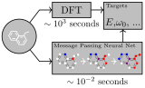
Figure 1: A Message Passing Neural Network predicts quantum properties of an organic molecule by modeling a computationally expensive DFT calculation.
图 1:消息传递神经网络通过模拟计算代价高昂的 DFT 计算,来预测有机分子的量子性质。
Recently, large scale quantum chemistry calculation and molecular dynamics simulations coupled with advances in high throughput experiments have begun to generate data at an unprecedented rate. Most classical techniques do not make effective use of the larger amounts of data that are now available. The time is ripe to apply more powerful and flexible machine learning methods to these problems, assuming we can find models with suitable inductive biases. The symmetries of atomic systems suggest neural networks that operate on graph structured data and are invariant to graph isomorphism might also be appropriate for molecules. Sufficiently successful models could someday help automate challenging chemical search problems in drug discovery or materials science.
近来,大规模量子化学计算和分子动力学模拟,加上高通量实验的进展,开始以前所未有的速度产生数据。大多数经典技术无法有效利用现在可得的大量数据。只要能找到具有合适归纳偏置的模型,现在正是把更强大、更灵活的机器学习方法用于这些问题的时机。原子系统的对称性提示我们,作用于图结构数据、对图同构(graph isomorphism)保持不变的神经网络,也可能适用于分子。足够成功的模型有朝一日可以帮助自动化药物发现或材料科学中困难的化学搜索问题。
In this paper, our goal is to demonstrate effective machine learning models for chemical prediction problems that are capable of learning their own features from molecular graphs directly and are invariant to graph isomorphism. To that end, we describe a general framework for supervised learning on graphs called Message Passing Neural Networks (MPNNs) that simply abstracts the commonalities between several of the most promising existing neural models for graph structured data, in order to make it easier to understand the relationships between them and come up with novel variations. Given how many researchers have published models that fit into the MPNN framework, we believe that the community should push this general approach as far as possible on practically important graph problems and only suggest new variations that are well motivated by applications, such as the application we consider here: predicting the quantum mechanical properties of small organic molecules (see task schematic in figure 1).
本文的目标是展示能有效解决化学预测问题的机器学习模型:它们能直接从分子图中学习自己的特征,并且对图同构保持不变。为此,我们描述了一个图上监督学习的通用框架,称为消息传递神经网络(MPNN)。它只是把现有几种最有前景的图结构数据神经模型的共同点抽象出来,以便更容易理解它们之间的关系,并提出新的变体。鉴于已有这么多研究者发表了符合 MPNN 框架的模型,我们认为学界应当在有实际意义的图问题上把这一通用方法推到极限,只提出由应用充分驱动的新变体,比如本文考虑的应用:预测小型有机分子的量子力学性质(任务示意见图 1)。
In general, the search for practically effective machine learning (ML) models in a given domain proceeds through a sequence of increasingly realistic and interesting benchmarks. Here we focus on the QM9 dataset as such a benchmark (Ramakrishnan et al. 2014). QM9 consists of 130k molecules with 13 properties for each molecule which are approximated by an expensive¹ quantum mechanical simulation method (DFT), to yield 13 corresponding regression tasks. These tasks are plausibly representative of many important chemical prediction problems and are (currently) difficult for many existing methods. Additionally, QM9 also includes complete spatial information for the single low energy conformation of the atoms in the molecule that was used in calculating the chemical properties. QM9 therefore lets us consider both the setting where the complete molecular geometry is known (atomic distances, bond angles, etc.) and the setting where we need to compute properties that might still be defined in terms of the spatial positions of atoms, but where only the atom and bond information (i.e. graph) is available as input. In the latter case, the model must implicitly fit something about the computation used to determine a low energy 3D conformation and hopefully would still work on problems where it is not clear how to compute a reasonable 3D conformation.
一般来说,在某个领域寻找实际有效的机器学习(ML)模型,要经过一系列越来越贴近现实、越来越有意思的基准。这里我们把 QM9 数据集(Ramakrishnan et al. 2014)作为这样一个基准。QM9 包含 13 万个分子,每个分子有 13 种性质,这些性质由一种昂贵的¹量子力学模拟方法(DFT)近似计算得到,构成 13 个相应的回归任务。这些任务很可能代表了许多重要的化学预测问题,而且(目前)对许多现有方法来说都很难。此外,QM9 还包含计算化学性质时所用的那个分子低能构象中原子的完整空间信息。因此,QM9 让我们既能考虑完整分子几何(原子间距离、键角等)已知的情形,也能考虑另一种情形:要计算的性质仍可能是由原子空间位置定义的,但输入只有原子和化学键信息(即图)。在后一种情况下,模型必须隐式拟合确定低能三维构象的那部分计算;我们希望,在不清楚如何计算合理三维构象的问题上,它依然有效。
By comparison, the inference time of the neural networks discussed in this work is 300k times faster.
相比之下,本文讨论的神经网络的推理速度快 30 万倍。
When measuring the performance of our models on QM9, there are two important benchmark error levels. The first is the estimated average error of the DFT approximation to nature, which we refer to as “DFT error.” The second, known as “chemical accuracy,” is a target error that has been established by the chemistry community. Estimates of DFT error and chemical accuracy are provided for each of the 13 targets in Faber et al. 2017. One important goal of this line of research is to produce a model which can achieve chemical accuracy with respect to the true targets as measured by an extremely precise experiment. The dataset containing the true targets on all 134k molecules does not currently exist. However, the ability to fit the DFT approximation to within chemical accuracy would be an encouraging step in this direction. For all 13 targets, achieving chemical accuracy is at least as hard as achieving DFT error. In the rest of this paper when we talk about chemical accuracy we generally mean with respect to our available ground truth labels.
衡量我们的模型在 QM9 上的表现时,有两个重要的基准误差水平。第一个是 DFT 近似相对于自然界的估计平均误差,我们称之为“DFT 误差”。第二个称为“化学精度”(chemical accuracy),是化学界确立的目标误差。Faber et al. 2017 为 13 个目标各自给出了 DFT 误差和化学精度的估计。这一研究方向的一个重要目标,是得到一个相对于由极其精确的实验测得的真实目标能达到化学精度的模型。目前还不存在包含全部 13.4 万个分子真实目标值的数据集。不过,能在化学精度以内拟合 DFT 近似,会是朝这个方向迈出的鼓舞人心的一步。对所有 13 个目标来说,达到化学精度至少与达到 DFT 误差一样难。本文其余部分提到化学精度时,一般指相对于我们现有的真值标签而言。
In this paper, by exploring novel variations of models in the MPNN family, we are able to both achieve a new state of the art on the QM9 dataset and to predict the DFT calculation to within chemical accuracy on all but two targets. In particular, we provide the following key contributions:
本文通过探索 MPNN 家族中模型的新变体,既在 QM9 数据集上取得了新的最先进结果,又在除两个目标以外的所有目标上把 DFT 计算预测到了化学精度以内。具体而言,我们的主要贡献如下:
- We develop an MPNN which achieves state of the art results on all 13 targets and predicts DFT to within chemical accuracy on 11 out of 13 targets.
- We develop several different MPNNs which predict DFT to within chemical accuracy on 5 out of 13 targets while operating on the topology of the molecule alone (with no spatial information as input).
- We develop a general method to train MPNNs with larger node representations without a corresponding increase in computation time or memory, yielding a substantial savings over previous MPNNs for high dimensional node representations.
- 我们开发了一个 MPNN,它在全部 13 个目标上取得最先进结果,并在 13 个目标中的 11 个上把 DFT 预测到化学精度以内。
- 我们开发了几种不同的 MPNN,它们只使用分子的拓扑结构(输入中没有空间信息),就在 13 个目标中的 5 个上把 DFT 预测到化学精度以内。
- 我们开发了一种通用方法,可以训练节点表示更大的 MPNN,而计算时间和内存不会相应增加;对于高维节点表示,这比以往的 MPNN 大幅节省开销。
We believe our work is an important step towards making well-designed MPNN’s the default for supervised learning on modestly sized molecules. In order for this to happen, researchers need to perform careful empirical studies to find the proper way to use these types of models and to make any necessary improvements to them, it is not sufficient for these models to have been described in the literature if there is only limited accompanying empirical work in the chemical domain. Indeed convolutional neural networks existed for decades before careful empirical work applying them to image classification (Krizhevsky et al. 2012) helped them displace SVMs on top of hand-engineered features for a host of computer vision problems.
我们相信,这项工作是让精心设计的 MPNN 成为中等大小分子监督学习默认选择的重要一步。要做到这一点,研究者需要开展仔细的实证研究,找出使用这类模型的恰当方式,并做出必要的改进;如果在化学领域只有有限的配套实证工作,仅仅在文献中描述这些模型是不够的。事实上,卷积神经网络存在了几十年,直到把它用于图像分类的细致实证工作(Krizhevsky et al. 2012)出现,才帮助它在大量计算机视觉问题上取代了基于手工特征的 SVM。
2 Message Passing Neural Networks
2 消息传递神经网络
There are at least eight notable examples of models from the literature that we can describe using our Message Passing Neural Networks (MPNN) framework. For simplicity we describe MPNNs which operate on undirected graphs with node features and edge features . It is trivial to extend the formalism to directed multigraphs. The forward pass has two phases, a message passing phase and a readout phase. The message passing phase runs for time steps and is defined in terms of message functions and vertex update functions . During the message passing phase, hidden states at each node in the graph are updated based on messages according to
文献中至少有八个值得注意的模型可以用我们的消息传递神经网络(MPNN)框架来描述。为简单起见,我们描述作用于无向图 的 MPNN,节点特征为 ,边特征为 。把这套形式推广到有向多重图是很直接的。前向传播分两个阶段:消息传递阶段和读出(readout)阶段。消息传递阶段运行 个时间步,由消息函数 和顶点更新函数 定义。在消息传递阶段,图中每个节点的隐藏状态 根据消息 按下式更新:
where in the sum, denotes the neighbors of in graph . The readout phase computes a feature vector for the whole graph using some readout function according to
其中求和中的 表示图 中 的邻居。读出阶段用某个读出函数 为整个图计算一个特征向量:
The message functions , vertex update functions , and readout function are all learned differentiable functions. operates on the set of node states and must be invariant to permutations of the node states in order for the MPNN to be invariant to graph isomorphism. In what follows, we define previous models in the literature by specifying the message function , vertex update function , and readout function used. Note one could also learn edge features in an MPNN by introducing hidden states for all edges in the graph and updating them analogously to equations 1 and 2. Of the existing MPNNs, only Kearnes et al. 2016 has used this idea.
消息函数 、顶点更新函数 和读出函数 都是学习得到的可微函数。 作用于节点状态的集合,并且必须对节点状态的排列保持不变,MPNN 才能对图同构保持不变。下面我们通过指定所用的消息函数 、顶点更新函数 和读出函数 ,来定义文献中已有的模型。注意,也可以在 MPNN 中学习边特征:为图中所有边引入隐藏状态 ,并仿照式 1 和式 2 更新它们。在现有的 MPNN 中,只有 Kearnes et al. 2016 使用了这个想法。
Convolutional Networks for Learning Molecular Fingerprints, Duvenaud et al. 2015
用于学习分子指纹的卷积网络(Convolutional Networks for Learning Molecular Fingerprints),Duvenaud et al. 2015
The message function used is where denotes concatenation. The vertex update function used is , where is the sigmoid function, deg is the degree of vertex and is a learned matrix for each time step and vertex degree . has skip connections to all previous hidden states and is equal to , where is a neural network and are learned readout matrices, one for each time step . This message passing scheme may be problematic since the resulting message vector is which separately sums over connected nodes and connected edges. It follows that the message passing implemented in Duvenaud et al. 2015 is unable to identify correlations between edge states and node states.
所用的消息函数是 ,其中 表示拼接。所用的顶点更新函数是 ,其中 是 sigmoid 函数,deg 是顶点 的度, 是针对每个时间步 和顶点度 学习的矩阵。 与之前所有隐藏状态 都有跳跃连接,等于 ,其中 是一个神经网络, 是学习得到的读出矩阵,每个时间步 一个。这种消息传递方式可能有问题,因为得到的消息向量是 它分别对相连的节点和相连的边求和。由此可知,Duvenaud et al. 2015 实现的消息传递无法识别边状态与节点状态之间的相关性。
Gated Graph Neural Networks (GG-NN), Li et al. 2016
门控图神经网络(Gated Graph Neural Networks,GG-NN),Li et al. 2016
The message function used is , where is a learned matrix, one for each edge label (the model assumes discrete edge types). The update function is , where GRU is the Gated Recurrent Unit introduced in Cho et al. 2014. This work used weight tying, so the same update function is used at each time step . Finally,
所用的消息函数是 ,其中 是学习得到的矩阵,每种边标签 一个(该模型假设边的类型是离散的)。更新函数是 ,其中 GRU 是 Cho et al. 2014 提出的门控循环单元(Gated Recurrent Unit)。这项工作使用了权重共享,因此每个时间步 都使用相同的更新函数。最后,
where and are neural networks, and denotes element-wise multiplication.
其中 和 是神经网络, 表示逐元素相乘。
Interaction Networks, Battaglia et al. 2016
交互网络(Interaction Networks),Battaglia et al. 2016
This work considered both the case where there is a target at each node in the graph, and where there is a graph level target. It also considered the case where there are node level effects applied at each time step, in such a case the update function takes as input the concatenation where is an external vector representing some outside influence on the vertex . The message function is a neural network which takes the concatenation . The vertex update function is a neural network which takes as input the concatenation . Finally, in the case where there is a graph level output, where is a neural network which takes the sum of the final hidden states . Note the original work only defined the model for .
这项工作既考虑了图中每个节点都有目标的情形,也考虑了只有图级目标的情形。它还考虑了每个时间步都施加节点级作用的情形,此时更新函数的输入是拼接 ,其中 是表示顶点 所受外部影响的外部向量。消息函数 是一个以拼接 为输入的神经网络。顶点更新函数 是一个以拼接 为输入的神经网络。最后,在有图级输出的情况下,,其中 是一个以最终隐藏状态 之和为输入的神经网络。注意,原工作只定义了 时的模型。
Molecular Graph Convolutions, Kearnes et al. 2016
分子图卷积(Molecular Graph Convolutions),Kearnes et al. 2016
This work deviates slightly from other MPNNs in that it introduces edge representations which are updated during the message passing phase. The message function used for node messages is . The vertex update function is where denotes concatenation, is the ReLU activation and are learned weight matrices. The edge state update is defined by where the are also learned weight matrices.
这项工作与其他 MPNN 略有不同:它引入了在消息传递阶段更新的边表示 。节点消息所用的消息函数是 。顶点更新函数是 ,其中 表示拼接, 是 ReLU 激活函数, 是学习得到的权重矩阵。边状态的更新定义为 ,其中 也是学习得到的权重矩阵。
Deep Tensor Neural Networks, Schütt et al. 2017
深度张量神经网络(Deep Tensor Neural Networks),Schütt et al. 2017
The message from to is computed by
从 到 的消息按下式计算:
where , , are matrices and , are bias vectors. The update function used is . The readout function passes each node independently through a single hidden layer neural network and sums the outputs, in particular
其中 、、 是矩阵,、 是偏置向量。所用的更新函数是 。读出函数让每个节点独立通过一个单隐藏层神经网络,再把输出相加,具体为
Laplacian Based Methods, Bruna et al. 2013; Defferrard et al. 2016; Kipf & Welling 2016
基于拉普拉斯矩阵的方法(Laplacian Based Methods),Bruna et al. 2013; Defferrard et al. 2016; Kipf & Welling 2016
These methods generalize the notion of the convolution operation typically applied to image datasets to an operation that operates on an arbitrary graph with a real valued adjacency matrix . The operations defined in Bruna et al. 2013; Defferrard et al. 2016 result in message functions of the form , where the matrices are parameterized by the eigenvectors of the graph laplacian , and the learned parameters of the model. The vertex update function used is where is some pointwise non-linearity (such as ReLU).
这些方法把通常用于图像数据集的卷积运算,推广到作用于任意图 的运算上,该图有一个实值邻接矩阵 。Bruna et al. 2013 和 Defferrard et al. 2016 定义的运算得到形如 的消息函数,其中矩阵 由图拉普拉斯矩阵 的特征向量和模型的学习参数共同参数化。所用的顶点更新函数是 ,其中 是某种逐点非线性(如 ReLU)。
The Kipf & Welling 2016 model results in a message function where . The vertex update function is . For the exact expressions for the and the derivation of the reformulation of these models as MPNNs, see the supplementary material.
Kipf & Welling 2016 的模型得到的消息函数是 ,其中 。顶点更新函数是 。 的精确表达式,以及把这些模型重新表述为 MPNN 的推导,见补充材料。
2.1 Moving Forward
2.1 下一步
Given how many instances of MPNN’s have appeared in the literature, we should focus on pushing this general family as far as possible in a specific application of substantial practical importance. This way we can determine the most crucial implementation details and potentially reach the limits of these models to guide us towards future modeling improvements.
既然文献中已经出现了这么多 MPNN 实例,我们应当在一个有重大实际意义的具体应用上,把这一通用家族推到极限。这样我们就能确定最关键的实现细节,并有可能触及这些模型的极限,从而指引未来的建模改进。
One downside of all of these approaches is computation time. Recent work has adapted the GG-NN architecture to larger graphs by passing messages on only subsets of the graph at each time step (Marino et al. 2016). In this work we also present a MPNN modification that can improve the computational costs.
所有这些方法的一个缺点是计算时间。近来有工作让 GG-NN 架构适应更大的图,做法是每个时间步只在图的子集上传递消息(Marino et al. 2016)。本文我们也提出一种能降低计算开销的 MPNN 改进。
3 Related Work
3 相关工作
Although in principle quantum mechanics lets us compute the properties of molecules, the laws of physics lead to equations that are far too difficult to solve exactly. Therefore scientists have developed a hierarchy of approximations to quantum mechanics with varying tradeoffs of speed and accuracy, such as Density Functional Theory (DFT) with a variety of functionals (Becke 1993; Hohenberg & Kohn 1964), the GW approximation (Hedin 1965), and Quantum Monte-Carlo (Ceperley & Alder 1986). Despite being widely used, DFT is simultaneously still too slow to be applied to large systems (scaling as where is the number of electrons) and exhibits systematic as well as random errors relative to exact solutions to Schrödinger’s equation. For example, to run the DFT calculation on a single 9 heavy atom molecule in QM9 takes around an hour on a single core of a Xeon E5-2660 (2.2 GHz) using a version of Gaussian G09 (ES64L-G09RevD.01) (Bing et al. 2017). For a 17 heavy atom molecule, computation time is up to 8 hours. Empirical potentials have been developed, such as the Stillinger-Weber potential (Stillinger & Weber 1985), that are fast and accurate but must be created from scratch, from first principles, for every new composition of atoms.
虽然原则上量子力学能让我们计算分子的性质,但物理定律导出的方程太难精确求解。因此,科学家发展了一系列量子力学近似,在速度与精度之间做出不同权衡,例如采用各种泛函的密度泛函理论(Density Functional Theory,DFT)(Becke 1993; Hohenberg & Kohn 1964)、GW 近似(Hedin 1965)和量子蒙特卡罗(Ceperley & Alder 1986)。DFT 虽然被广泛使用,但对大体系仍然太慢(复杂度为 , 是电子数),而且相对于薛定谔方程的精确解既有系统误差也有随机误差。例如,用某个版本的 Gaussian G09(ES64L-G09RevD.01)在 Xeon E5-2660(2.2 GHz)的单核上,对 QM9 中一个含 9 个重原子的分子做 DFT 计算大约需要一小时(Bing et al. 2017)。对含 17 个重原子的分子,计算时间可达 8 小时。人们还开发了经验势,例如 Stillinger-Weber 势(Stillinger & Weber 1985),它们快速又准确,但每遇到一种新的原子组成,都必须从第一性原理出发从头构建。
Hu et al. 2003 used neural networks to approximate a particularly troublesome term in DFT called the exchange correlation potential to improve the accuracy of DFT. However, their method fails to improve upon the efficiency of DFT and relies on a large set of ad hoc atomic descriptors.
Hu et al. 2003 用神经网络近似 DFT 中一个特别麻烦的项,即交换关联势(exchange correlation potential),以提高 DFT 的精度。然而,他们的方法没有提升 DFT 的效率,并依赖一大套临时拼凑的原子描述符。
Two more recent approaches by Behler & Parrinello 2007 and Rupp et al. 2012 attempt to approximate solutions to quantum mechanics directly without appealing to DFT. In the first case single-hidden-layer neural networks were used to approximate the energy and forces for configurations of a Silicon melt with the goal of speeding up molecular dynamics simulations. The second paper used Kernel Ridge Regression (KRR) to infer atomization energies over a wide range of molecules. In both cases hand engineered features were used (symmetry functions and the Coulomb matrix, respectively) that built physical symmetries into the input representation. Subsequent papers have replaced KRR by a neural network.
Behler & Parrinello 2007 和 Rupp et al. 2012 这两种较新的方法,尝试绕开 DFT 直接近似量子力学的解。前者用单隐藏层神经网络近似硅熔体各种构型的能量和受力,目的是加速分子动力学模拟。后者用核岭回归(Kernel Ridge Regression,KRR)推断大量分子的原子化能。两者都使用了手工设计的特征(分别是对称函数和库仑矩阵),把物理对称性内置到输入表示中。后续论文用神经网络取代了 KRR。
Both of these lines of research used hand engineered features that have intrinsic limitations. The work of Behler & Parrinello 2007 used a representation that was manifestly invariant to graph isomorphism, but has difficulty when applied to systems with more than three species of atoms and fails to generalize to novel compositions. The representation used in Rupp et al. 2012 is not invariant to graph isomorphism. Instead, this invariance must be learned by the downstream model through dataset augmentation.
这两条研究路线使用的手工特征都有内在局限。Behler & Parrinello 2007 使用的表示显然对图同构不变,但用于原子种类超过三种的体系时有困难,也无法泛化到新的组成。Rupp et al. 2012 使用的表示对图同构并不保持不变,这种不变性必须由下游模型通过数据增强来学习。
In addition to the eight MPNN’s discussed in Section 2 there have been a number of other approaches to machine learning on graphical data which take advantage of the symmetries in a number of ways. One such family of approaches define a preprocessing step which constructs a canonical graph representation which can then be fed into into a standard classifier. Examples in this family include Niepert et al. 2016 and Rupp et al. 2012. Finally Scarselli et al. 2009 define a message passing process on graphs which is run until convergence, instead of for a finite number of time steps as in MPNNs.
除了第 2 节讨论的八个 MPNN,还有许多其他针对图数据的机器学习方法,以不同方式利用对称性。其中一类方法定义一个预处理步骤,构造规范的图表示,再输入标准分类器。这一类的例子包括 Niepert et al. 2016 和 Rupp et al. 2012。最后,Scarselli et al. 2009 在图上定义了一个运行到收敛为止的消息传递过程,而不像 MPNN 那样只运行有限个时间步。
4 QM9 Dataset
4 QM9 数据集
To investigate the success of MPNNs on predicting chemical properties, we use the publicly available QM9 dataset (Ramakrishnan et al. 2014). Molecules in the dataset consist of Hydrogen (H), Carbon (C), Oxygen (O), Nitrogen (N), and Flourine (F) atoms and contain up to 9 heavy (non Hydrogen) atoms. In all, this results in about 134k drug-like organic molecules that span a wide range of chemistry. For each molecule DFT is used to find a reasonable low energy structure and hence atom “positions” are available. Additionally a wide range of interesting and fundamental chemical properties are computed. Given how fundamental some of the QM9 properties are, it is hard to believe success on more challenging chemical tasks will be possible if we can’t make accurate statistical predictions for the properties computed in QM9.
为了考察 MPNN 预测化学性质的效果,我们使用公开的 QM9 数据集(Ramakrishnan et al. 2014)。数据集中的分子由氢(H)、碳(C)、氧(O)、氮(N)和氟(F)原子组成,最多含 9 个重原子(非氢原子)。总计约 13.4 万个类药有机分子,覆盖广泛的化学范围。对每个分子,都用 DFT 找到一个合理的低能结构,因此可以得到原子的“位置”。此外还计算了多种有意思的基本化学性质。鉴于 QM9 中某些性质如此基础,如果我们连 QM9 中计算的这些性质都无法做出准确的统计预测,很难相信能在更有挑战的化学任务上取得成功。
We can group the different properties we try to predict into four broad categories. First, we have four properties related to how tightly bound together the atoms in a molecule are. These measure the energy required to break up the molecule at different temperatures and pressures. These include the atomization energy at , (eV), atomization energy at room temperature, (eV), enthalpy of atomization at room temperature, (eV), and free energy of atomization, (eV).
我们要预测的性质可以分为四大类。第一类是与分子中原子结合紧密程度有关的四种性质,它们衡量在不同温度和压强下拆散分子所需的能量,包括 时的原子化能 (eV)、室温下的原子化能 (eV)、室温下的原子化焓 (eV),以及原子化自由能 (eV)。
Next there are properties related to fundamental vibrations of the molecule, including the highest fundamental vibrational frequency () and the zero point vibrational energy (ZPVE) (eV).
其次是与分子基本振动有关的性质,包括最高基本振动频率 ()和零点振动能(ZPVE)(eV)。
Additionally, there are a number of properties that concern the states of the electrons in the molecule. They include the energy of the electron in the highest occupied molecular orbital (HOMO) (eV), the energy of the lowest unoccupied molecular orbital (LUMO) (eV), and the electron energy gap ( (eV)). The electron energy gap is simply the difference .
此外,还有一些与分子中电子状态有关的性质,包括最高占据分子轨道(HOMO)中电子的能量 (eV)、最低未占分子轨道(LUMO)的能量 (eV),以及电子能隙((eV))。电子能隙就是二者之差 。
Finally, there are several measures of the spatial distribution of electrons in the molecule. These include the electronic spatial extent (Bohr²), the norm of the dipole moment (Debye), and the norm of static polarizability (Bohr³). For a more detailed description of these properties, see the supplementary material.
最后,还有几种衡量分子中电子空间分布的量,包括电子空间范围 (Bohr²)、偶极矩的模 (Debye),以及静态极化率的模 (Bohr³)。这些性质的详细说明见补充材料。
5 MPNN Variants
5 MPNN 变体
We began our exploration of MPNNs around the GG-NN model which we believe to be a strong baseline. We focused on trying different message functions, output functions, finding the appropriate input representation, and properly tuning hyperparameters.
我们以 GG-NN 模型为中心开始探索 MPNN,我们认为它是一个强基线。我们重点尝试了不同的消息函数和输出函数,寻找合适的输入表示,并仔细调节超参数。
For the rest of the paper we use to denote the dimension of the internal hidden representation of each node in the graph, and to denote the number of nodes in the graph. Our implementation of MPNNs in general operates on directed graphs with a separate message channel for incoming and outgoing edges, in which case the incoming message is the concatenation of and , this was also used in Li et al. 2016. When we apply this to undirected chemical graphs we treat the graph as directed, where each original edge becomes both an incoming and outgoing edge with the same label. Note there is nothing special about the direction of the edge, it is only relevant for parameter tying. Treating undirected graphs as directed means that the size of the message channel is instead of .
本文其余部分用 表示图中每个节点内部隐藏表示的维度,用 表示图中的节点数。我们的 MPNN 实现一般作用于有向图,入边和出边各有一个独立的消息通道,此时传入消息 是 和 的拼接;Li et al. 2016 也使用了这种做法。把它用于无向的化学图时,我们把图当作有向图处理,每条原始边同时成为一条入边和一条出边,标签相同。注意,边的方向并没有什么特别之处,只与参数共享有关。把无向图当作有向图处理,意味着消息通道的大小是 而不是 。
The input to our MPNN model is a set of feature vectors for the nodes of the graph, , and an adjacency matrix with vector valued entries to indicate different bonds in the molecule as well as pairwise spatial distance between two atoms. We experimented as well with the message function used in the GG-NN family, which assumes discrete edge labels, in which case the matrix has entries in a discrete alphabet of size . The initial hidden states are set to be the atom input feature vectors and are padded up to some larger dimension . All of our experiments used weight tying at each time step , and a GRU (Cho et al. 2014) for the update function as in the GG-NN family.
我们的 MPNN 模型的输入是图中各节点的特征向量 ,以及一个邻接矩阵 ; 的元素是向量,用来表示分子中不同的化学键以及两个原子之间的空间距离。我们也试验了 GG-NN 家族所用的消息函数,它假设边标签是离散的,此时矩阵 的元素取自大小为 的离散字母表。初始隐藏状态 设为原子的输入特征向量 ,并填充到某个更大的维度 。我们所有实验都在各时间步 之间共享权重,并像 GG-NN 家族一样用 GRU(Cho et al. 2014)作为更新函数。
5.1 Message Functions
5.1 消息函数
Matrix Multiplication: We started with the message function used in GG-NN which is defined by the equation .
矩阵乘法(Matrix Multiplication):我们从 GG-NN 所用的消息函数开始,其定义为 。
Edge Network: To allow vector valued edge features we propose the message function where is a neural network which maps the edge vector to a matrix.
边网络(Edge Network):为了支持向量值的边特征,我们提出消息函数 ,其中 是一个神经网络,把边向量 映射为一个 矩阵。
Pair Message: One property that the matrix multiplication rule has is that the message from node to node is a function only of the hidden state and the edge . In particular, it does not depend on the hidden state . In theory, a network may be able to use the message channel more efficiently if the node messages are allowed to depend on both the source and destination node. Thus we also tried using a variant on the message function as described in (Battaglia et al. 2016). Here the message from to along edge is where is a neural network.
成对消息(Pair Message):矩阵乘法规则有一个性质:从节点 到节点 的消息只是隐藏状态 和边 的函数。特别是,它不依赖于隐藏状态 。理论上,如果允许节点消息同时依赖源节点和目标节点,网络或许能更有效地利用消息通道。因此我们也尝试了(Battaglia et al. 2016)中所述消息函数的一个变体。这里,沿边 从 到 的消息是 ,其中 是一个神经网络。
When we apply the above message functions to directed graphs, there are two separate functions used, and an . Which function is applied to a particular edge depends on the direction of that edge.
把上述消息函数用于有向图时,会使用两个独立的函数 和 。对某条边 使用哪个函数,取决于这条边的方向。
5.2 Virtual Graph Elements
5.2 虚拟图元素
We explored two different ways to change how the messages are passed throughout the model. The simplest modification involves adding a separate “virtual” edge type for pairs of nodes that are not connected. This can be implemented as a data preprocessing step and allows information to travel long distances during the propagation phase.
我们探索了两种改变消息在模型中传递方式的方法。最简单的改动是为不相连的节点对添加一种单独的“虚拟”边类型。这可以作为数据预处理步骤来实现,并让信息在传播阶段传得更远。
We also experimented with using a latent “master” node, which is connected to every input node in the graph with a special edge type. The master node serves as a global scratch space that each node both reads from and writes to in every step of message passing. We allow the master node to have a separate node dimension , as well as separate weights for the internal update function (in our case a GRU). This allows information to travel long distances during the propagation phase. It also, in theory, allows additional model capacity (e.g. large values of ) without a substantial hit in performance, as the complexity of the master node model is .
我们还试验了一个隐含的“主”节点(master node),它通过一种特殊的边类型与图中每个输入节点相连。主节点充当全局草稿区,每一步消息传递中,每个节点都既从它读取、也向它写入。我们允许主节点有单独的节点维度 ,以及内部更新函数(我们这里是 GRU)的单独权重。这让信息在传播阶段可以传得更远。理论上,它还允许增加模型容量(例如取较大的 )而不会明显影响性能,因为主节点模型的复杂度是 。
5.3 Readout Functions
5.3 读出函数
We experimented with two readout functions. First is the readout function used in GG-NN, which is defined by equation 4. Second is a set2set model from Vinyals et al. 2015. The set2set model is specifically designed to operate on sets and should have more expressive power than simply summing the final node states. This model first applies a linear projection to each tuple () and then takes as input the set of projected tuples . Then, after steps of computation, the set2set model produces a graph level embedding which is invariant to the order of the of the tuples . We feed this embedding through a neural network to produce the output.
我们试验了两种读出函数。第一种是 GG-NN 所用的读出函数,由式 4 定义。第二种是 Vinyals et al. 2015 的 set2set 模型。set2set 模型专为作用于集合而设计,应当比简单地对最终节点状态求和有更强的表达能力。这个模型先对每个元组()做线性投影,再以投影后的元组集合 为输入。经过 步计算后,set2set 模型产生一个图级嵌入 ,它与元组集合 的顺序无关。我们把嵌入 送入一个神经网络得到输出。
5.4 Multiple Towers
5.4 多塔结构
One issue with MPNN’s is scalability. In particular, a single step of the message passing phase for a dense graph requires floating point multiplications. As or get large this can be computationally expensive. To address this issue we break the dimensional node embeddings into different dimensional embeddings and run a propagation step on each of the copies separately to get temporary embeddings , using separate message and update functions for each copy. The temporary embeddings of each node are then mixed together according to the equation
MPNN 的一个问题是可扩展性。特别是,对稠密图来说,消息传递阶段的一步需要 次浮点乘法。当 或 变大时,计算代价可能很高。为了解决这个问题,我们把 维节点嵌入 拆成 个不同的 维嵌入 ,对 份副本分别运行一步传播,各副本使用独立的消息函数和更新函数,得到临时嵌入 。然后按下式把每个节点的 个临时嵌入混合在一起:
where denotes a neural network and denotes concatenation, with shared across all nodes in the graph. This mixing preserves the invariance to permutations of the nodes, while allowing the different copies of the graph to communicate with each other during the propagation phase. This can be advantageous in that it allows larger hidden states for the same number of parameters, which yields a computational speedup in practice. For example, when the message function is matrix multiplication (as in GG-NN) a propagation step of a single copy takes time, and there are copies, therefore the overall time complexity is , with some additional overhead due to the mixing network. For , and we see a factor of 2 speedup in inference time over a , , and architecture. This variation would be most useful for larger molecules, for instance molecules from GDB-17 (Ruddigkeit et al. 2012).
其中 表示一个神经网络, 表示拼接, 在图中所有节点间共享。这种混合保持了对节点排列的不变性,同时允许图的不同副本在传播阶段相互通信。它的好处是,在参数量相同的情况下可以使用更大的隐藏状态,实践中带来计算加速。例如,当消息函数是矩阵乘法时(如 GG-NN),单个副本的一步传播需要 时间,共有 个副本,因此总时间复杂度是 ,另有混合网络带来的一些额外开销。对于 、、,我们观察到推理时间比 、、 的架构快 2 倍。这种变体对更大的分子最有用,例如 GDB-17 中的分子(Ruddigkeit et al. 2012)。
6 Input Representation
6 输入表示
There are a number of features available for each atom in a molecule which capture both properties of the electrons in the atom as well as the bonds that the atom participates in. For a list of all of the features see table 1. We experimented with making the hydrogen atoms explicit nodes in the graph (as opposed to simply including the count as a node feature), in which case graphs have up to 29 nodes. Note that having larger graphs significantly slows training time, in this case by a factor of roughly 10. For the adjacency matrix there are three edge representations used depending on the model.
分子中的每个原子都有许多可用特征,既刻画原子中电子的性质,也刻画该原子参与的化学键。全部特征见表 1。我们试验了把氢原子作为图中的显式节点(而不是只把氢原子数作为节点特征),此时图最多有 29 个节点。注意,更大的图会显著拖慢训练,这里大约慢了 10 倍。对于邻接矩阵,根据模型不同,使用三种边表示。
| Feature | Description |
|---|---|
| Atom type | H, C, N, O, F (one-hot) |
| Atomic number | Number of protons (integer) |
| Acceptor | Accepts electrons (binary) |
| Donor | Donates electrons (binary) |
| Aromatic | In an aromatic system (binary) |
| Hybridization | sp, sp2, sp3 (one-hot or null) |
| Number of Hydrogens | (integer) |
Table 1: Atom Features
| 特征 | 说明 |
|---|---|
| 原子类型 | H、C、N、O、F(独热编码) |
| 原子序数 | 质子数(整数) |
| 受体 | 接受电子(二值) |
| 供体 | 给出电子(二值) |
| 芳香性 | 处于芳香体系中(二值) |
| 杂化方式 | sp、sp2、sp3(独热编码或空) |
| 氢原子数 | (整数) |
表 1:原子特征
Chemical Graph: In the abscence of distance information, adjacency matrix entries are discrete bond types: single, double, triple, or aromatic.
化学图(Chemical Graph):在没有距离信息时,邻接矩阵的元素是离散的化学键类型:单键、双键、三键或芳香键。
Distance bins: The matrix multiply message function assumes discrete edge types, so to include distance information we bin bond distances into 10 bins, the bins are obtained by uniformly partitioning the interval into 8 bins, followed by adding a bin and . These bins were hand chosen by looking at a histogram of all distances. The adjacency matrix then has entries in an alphabet of size 14, indicating bond type for bonded atoms and distance bin for atoms that are not bonded. We found the distance for bonded atoms to be almost completely determined by bond type.
距离分箱(Distance bins):矩阵乘法消息函数假设边类型离散,因此为了纳入距离信息,我们把键长分到 10 个箱中:把区间 均匀分成 8 个箱,再加上 和 两个箱。这些箱是看过所有距离的直方图后手工选定的。于是邻接矩阵的元素取自大小为 14 的字母表,对成键原子表示键的类型,对不成键的原子表示距离所在的箱。我们发现,成键原子之间的距离几乎完全由键的类型决定。
Raw distance feature: When using a message function which operates on vector valued edges, the entries of the adjacency matrix are then 5 dimensional, where the first dimension indicates the euclidean distance between the pair of atoms, and the remaining four are a one-hot encoding of the bond type.
原始距离特征(Raw distance feature):使用作用于向量值边的消息函数时,邻接矩阵的元素是 5 维的:第一维表示两个原子之间的欧氏距离,其余四维是键类型的独热编码。
7 Training
7 训练
Each model and target combination was trained using a uniform random hyper parameter search with 50 trials. was constrained to be in the range (in practice, any works). The number of set2set computations was chosen from the range . All models were trained using SGD with the ADAM optimizer (Kingma & Ba 2014), with batch size 20 for 3 million steps (540 epochs). The initial learning rate was chosen uniformly between and . We used a linear learning rate decay that began between 10% and 90% of the way through training and the initial learning rate decayed to a final learning rate , using a decay factor in the range .
每种模型与目标的组合,都用 50 次试验的均匀随机超参数搜索来训练。 限定在 范围内(实践中任何 都可以)。set2set 的计算步数 从 中选择。所有模型都用 SGD 配合 ADAM 优化器(Kingma & Ba 2014)训练,批大小为 20,训练 300 万步(540 个 epoch)。初始学习率在 和 之间均匀选取。我们使用线性学习率衰减,衰减在训练进程的 10% 到 90% 之间某处开始,初始学习率 衰减到最终学习率 ,衰减因子 取值范围为 。
The QM-9 dataset has 130462 molecules in it. We randomly chose 10000 samples for validation, 10000 samples for testing, and used the rest for training. We use the validation set to do early stopping and model selection and we report scores on the test set. All targets were normalized to have mean 0 and variance 1. We minimize the mean squared error between the model output and the target, although we evaluate mean absolute error.
QM-9 数据集包含 130462 个分子。我们随机选 10000 个样本做验证、10000 个样本做测试,其余用于训练。我们用验证集做早停和模型选择,并报告测试集上的分数。所有目标都标准化为均值 0、方差 1。我们最小化模型输出与目标之间的均方误差,但用平均绝对误差来评估。
8 Results
8 结果
In all of our tables we report the ratio of the mean absolute error (MAE) of our models with the provided estimate of chemical accuracy for that target. Thus any model with error ratio less than 1 has achieved chemical accuracy for that target. In the supplementary material we list the chemical accuracy estimates for each target, these are the same estimates that were given in Faber et al. 2017. In this way, the MAE of our models can be calculated as . Note, unless otherwise indicated, all tables display result of models trained individually on each target (as opposed to training one model to predict all 13).
所有表格中,我们报告的都是模型平均绝对误差(MAE)与该目标化学精度估计值之比。因此,误差比小于 1 的模型就在该目标上达到了化学精度。补充材料列出了每个目标的化学精度估计值,与 Faber et al. 2017 给出的估计相同。这样,我们模型的 MAE 可以按 (误差比 × 化学精度)计算。注意,除非另有说明,所有表格展示的都是针对每个目标单独训练的模型的结果(而不是训练一个模型同时预测全部 13 个目标)。
| Target | BAML | BOB | CM | ECFP4 | HDAD | GC | GG-NN | DTNN | enn-s2s | enn-s2s-ens5 |
|---|---|---|---|---|---|---|---|---|---|---|
| mu | 4.34 | 4.23 | 4.49 | 4.82 | 3.34 | 0.70 | 1.22 | - | 0.30 | 0.20 |
| alpha | 3.01 | 2.98 | 4.33 | 34.54 | 1.75 | 2.27 | 1.55 | - | 0.92 | 0.68 |
| HOMO | 2.20 | 2.20 | 3.09 | 2.89 | 1.54 | 1.18 | 1.17 | - | 0.99 | 0.74 |
| LUMO | 2.76 | 2.74 | 4.26 | 3.10 | 1.96 | 1.10 | 1.08 | - | 0.87 | 0.65 |
| gap | 3.28 | 3.41 | 5.32 | 3.86 | 2.49 | 1.78 | 1.70 | - | 1.60 | 1.23 |
| R2 | 3.25 | 0.80 | 2.83 | 90.68 | 1.35 | 4.73 | 3.99 | - | 0.15 | 0.14 |
| ZPVE | 3.31 | 3.40 | 4.80 | 241.58 | 1.91 | 9.75 | 2.52 | - | 1.27 | 1.10 |
| U0 | 1.21 | 1.43 | 2.98 | 85.01 | 0.58 | 3.02 | 0.83 | - | 0.45 | 0.33 |
| U | 1.22 | 1.44 | 2.99 | 85.59 | 0.59 | 3.16 | 0.86 | - | 0.45 | 0.34 |
| H | 1.22 | 1.44 | 2.99 | 86.21 | 0.59 | 3.19 | 0.81 | - | 0.39 | 0.30 |
| G | 1.20 | 1.42 | 2.97 | 78.36 | 0.59 | 2.95 | 0.78 | .84² | 0.44 | 0.34 |
| Cv | 1.64 | 1.83 | 2.36 | 30.29 | 0.88 | 1.45 | 1.19 | - | 0.80 | 0.62 |
| Omega | 0.27 | 0.35 | 1.32 | 1.47 | 0.34 | 0.32 | 0.53 | - | 0.19 | 0.15 |
| Average | 2.17 | 2.08 | 3.37 | 53.97 | 1.35 | 2.59 | 1.36 | - | 0.68 | 0.52 |
Table 2: Comparison of Previous Approaches (left) with MPNN baselines (middle) and our methods (right)
| 目标 | BAML | BOB | CM | ECFP4 | HDAD | GC | GG-NN | DTNN | enn-s2s | enn-s2s-ens5 |
|---|---|---|---|---|---|---|---|---|---|---|
| mu | 4.34 | 4.23 | 4.49 | 4.82 | 3.34 | 0.70 | 1.22 | - | 0.30 | 0.20 |
| alpha | 3.01 | 2.98 | 4.33 | 34.54 | 1.75 | 2.27 | 1.55 | - | 0.92 | 0.68 |
| HOMO | 2.20 | 2.20 | 3.09 | 2.89 | 1.54 | 1.18 | 1.17 | - | 0.99 | 0.74 |
| LUMO | 2.76 | 2.74 | 4.26 | 3.10 | 1.96 | 1.10 | 1.08 | - | 0.87 | 0.65 |
| gap | 3.28 | 3.41 | 5.32 | 3.86 | 2.49 | 1.78 | 1.70 | - | 1.60 | 1.23 |
| R2 | 3.25 | 0.80 | 2.83 | 90.68 | 1.35 | 4.73 | 3.99 | - | 0.15 | 0.14 |
| ZPVE | 3.31 | 3.40 | 4.80 | 241.58 | 1.91 | 9.75 | 2.52 | - | 1.27 | 1.10 |
| U0 | 1.21 | 1.43 | 2.98 | 85.01 | 0.58 | 3.02 | 0.83 | - | 0.45 | 0.33 |
| U | 1.22 | 1.44 | 2.99 | 85.59 | 0.59 | 3.16 | 0.86 | - | 0.45 | 0.34 |
| H | 1.22 | 1.44 | 2.99 | 86.21 | 0.59 | 3.19 | 0.81 | - | 0.39 | 0.30 |
| G | 1.20 | 1.42 | 2.97 | 78.36 | 0.59 | 2.95 | 0.78 | .84² | 0.44 | 0.34 |
| Cv | 1.64 | 1.83 | 2.36 | 30.29 | 0.88 | 1.45 | 1.19 | - | 0.80 | 0.62 |
| Omega | 0.27 | 0.35 | 1.32 | 1.47 | 0.34 | 0.32 | 0.53 | - | 0.19 | 0.15 |
| 平均 | 2.17 | 2.08 | 3.37 | 53.97 | 1.35 | 2.59 | 1.36 | - | 0.68 | 0.52 |
表 2:以往方法(左)与 MPNN 基线(中)及我们的方法(右)的比较
As reported in Schütt et al. 2017. The model was trained on a different train/test split with 100k training samples vs 110k used in our experiments.
数据取自 Schütt et al. 2017。该模型使用了不同的训练/测试划分,训练样本为 10 万个,而我们的实验使用 11 万个。
| Model | Average Error Ratio |
|---|---|
| GG-NN | 3.47 |
| GG-NN + Virtual Edge | 2.90 |
| GG-NN + Master Node | 2.62 |
| GG-NN + set2set | 2.57 |
Table 3: Models Trained Without Spatial Information
| 模型 | 平均误差比 |
|---|---|
| GG-NN | 3.47 |
| GG-NN + 虚拟边 | 2.90 |
| GG-NN + 主节点 | 2.62 |
| GG-NN + set2set | 2.57 |
表 3:不使用空间信息训练的模型
| Model | Average Error Ratio |
|---|---|
| GG-NN + joint training | 1.92 |
| towers8 + joint training | 1.75 |
| GG-NN + individual training | 1.53 |
| towers8 + individual training | 1.37 |
Table 4: Towers vs Vanilla GG-NN (no explicit hydrogen)
| 模型 | 平均误差比 |
|---|---|
| GG-NN + 联合训练 | 1.92 |
| towers8 + 联合训练 | 1.75 |
| GG-NN + 单独训练 | 1.53 |
| towers8 + 单独训练 | 1.37 |
表 4:多塔结构与原始 GG-NN 的比较(不含显式氢原子)
We performed numerous experiments in order to find the best possible MPNN on this dataset as well as the proper input representation. In our experiments, we found that including the complete edge feature vector (bond type, spatial distance) and treating hydrogen atoms as explicit nodes in the graph to be very important for a number of targets. We also found that training one model per target consistently outperformed jointly training on all 13 targets. In some cases the improvement was up to 40%. Our best MPNN variant used the edge network message function, set2set output, and operated on graphs with explicit hydrogens. We were able to further improve performance on the test set by ensembling the predictions of the five models with lowest validation error.
我们做了大量实验,以找到这个数据集上最好的 MPNN 以及合适的输入表示。实验发现,对许多目标来说,纳入完整的边特征向量(键类型、空间距离)并把氢原子作为图中的显式节点非常重要。我们还发现,每个目标单独训练一个模型,始终优于在全部 13 个目标上联合训练,有些情况下提升达 40%。我们最好的 MPNN 变体使用边网络消息函数、set2set 输出,并作用于含显式氢原子的图。把验证误差最低的五个模型的预测做集成,还能进一步提升测试集上的表现。
In table 2 we compare the performance of our best MPNN variant (denoted with enn-s2s) and the corresponding ensemble (denoted with enn-s2s-ens5) with the previous state of the art on this dataset as reported in Faber et al. 2017. For clarity the error ratios of the best non-ensemble models are shown in bold. This previous work performed a comparison study of several existing ML models for QM9 and we have taken care to use the same train, validation, and test split. These baselines include 5 different hand engineered molecular representations, which then get fed through a standard, off-the-shelf classifier. These input representations include the Coulomb Matrix (CM, Rupp et al. 2012), Bag of Bonds (BoB, Hansen et al. 2015), Bonds Angles, Machine Learning (BAML, Huang & von Lilienfeld 2016), Extended Connectivity Fingerprints (ECPF4, Rogers & Hahn 2010), and “Projected Histograms” (HDAD, Faber et al. 2017) representations. In addition to these hand engineered features we include two existing baseline MPNNs, the Molecular Graph Convolutions model (GC) from Kearnes et al. 2016, and the original GG-NN model Li et al. 2016 trained with distance bins. Overall, our new MPNN achieves chemical accuracy on 11 out of 13 targets and state of the art on all 13 targets.
表 2 把我们最好的 MPNN 变体(记为 enn-s2s)及相应的集成(记为 enn-s2s-ens5),与 Faber et al. 2017 报告的该数据集上以往的最先进结果进行比较。为清楚起见,最好的非集成模型的误差比用粗体表示。那项工作对 QM9 上几种现有的机器学习模型做了比较研究,我们特意使用了相同的训练、验证和测试划分。这些基线包括 5 种不同的手工分子表示,再输入标准的现成分类器。这些输入表示包括库仑矩阵(CM,Rupp et al. 2012)、键袋(Bag of Bonds,BoB,Hansen et al. 2015)、键角机器学习(Bonds Angles, Machine Learning,BAML,Huang & von Lilienfeld 2016)、扩展连通性指纹(Extended Connectivity Fingerprints,ECPF4,Rogers & Hahn 2010)以及“投影直方图”(HDAD,Faber et al. 2017)。除了这些手工特征,我们还纳入了两个现有的 MPNN 基线:Kearnes et al. 2016 的分子图卷积模型(GC),以及用距离分箱训练的原始 GG-NN 模型(Li et al. 2016)。总体而言,我们的新 MPNN 在 13 个目标中的 11 个上达到化学精度,并在全部 13 个目标上取得最先进结果。
Training Without Spatial Information: We also experimented in the setting where spatial information is not included in the input. In general, we find that augmenting the MPNN with some means of capturing long range interactions between nodes in the graph greatly improves performance in this setting. To demonstrate this we performed 4 experiments, one where we train the GG-NN model on the sparse graph, one where we add virtual edges, one where we add a master node, and one where we change the graph level output to a set2set output. The error ratios averaged across the 13 targets are shown in table 3. Overall, these three modifications help on all 13 targets, and the Set2Set output achieves chemical accuracy on 5 out of 13 targets. For more details, consult the supplementary material. The experiments shown tables 3 and 4 were run with a partial charge feature as a node input. This feature is an output of the DFT calculation and thus could not be used in an applied setting. The state of art numbers we report in table 2 do not use this feature.
不使用空间信息的训练:我们还试验了输入中不包含空间信息的设定。总体而言,我们发现在这种设定下,给 MPNN 加上某种捕获图中节点之间长程相互作用的手段,能大幅提升性能。为了说明这一点,我们做了 4 组实验:一组在稀疏图上训练 GG-NN 模型,一组加入虚拟边,一组加入主节点,还有一组把图级输出换成 set2set 输出。13 个目标上平均的误差比见表 3。总体而言,这三种改动在全部 13 个目标上都有帮助,其中 Set2Set 输出在 13 个目标中的 5 个上达到化学精度。更多细节见补充材料。表 3 和表 4 中的实验把部分电荷特征作为节点输入。这个特征是 DFT 计算的输出,因此无法在实际应用中使用。我们在表 2 中报告的最先进数值没有使用这个特征。
Towers: Our original intent in developing the towers variant was to improve training time, as well as to allow the model to be trained on larger graphs. However, we also found some evidence that the multi-tower structure improves generalization performance. In table 4 we compare GG-NN + towers + set2set output vs a baseline GG-NN + set2set output when distance bins are used. We do this comparison in both the joint training regime and when training one model per target. The towers model outperforms the baseline model on 12 out of 13 targets in both individual and joint target training. We believe the benefit of towers is that it resembles training an ensemble of models. Unfortunately, our attempts so far at combining the towers and edge network message function have failed to further improve performance, possibly because the combination makes training more difficult. Further training details, and error ratios on all targets can be found in the supplementary material.
多塔结构(Towers):我们开发多塔变体的初衷,是缩短训练时间,并让模型能在更大的图上训练。不过,我们也发现一些证据表明,多塔结构能提升泛化性能。表 4 在使用距离分箱的条件下,比较了 GG-NN + 多塔 + set2set 输出与基线 GG-NN + set2set 输出。我们在联合训练和每个目标单独训练两种方式下都做了比较。无论单独训练还是联合训练,多塔模型都在 13 个目标中的 12 个上优于基线模型。我们认为多塔的好处在于它类似于训练一个模型集成。遗憾的是,我们迄今把多塔与边网络消息函数结合起来的尝试,都没能进一步提升性能,可能是因为这种组合让训练更困难。更多训练细节和所有目标上的误差比见补充材料。
Additional Experiments: In preliminary experiments, we tried disabling weight tying across different time steps. However, we found that the most effective way to increase performance was to tie the weights and use a larger hidden dimension . We also early on found the pair message function to perform worse than the edge network function. This included a toy pathfinding problem which was originally designed to benefit from using pair messages. Also, when trained jointly on the 13 targets the edge network function outperforms pair message on 11 out of 13 targets, and has an average error ratio of 1.53 compared to 3.98 for pair message. Given the difficulties with training this function we did not pursue it further. For performance on smaller sized training sets, consult the supplementary material.
其他实验:在初步实验中,我们尝试过取消不同时间步之间的权重共享。但我们发现,提升性能最有效的办法是共享权重并使用更大的隐藏维度 。我们也很早就发现成对消息函数不如边网络函数,包括在一个原本就是为发挥成对消息优势而设计的玩具寻路问题上。此外,在 13 个目标上联合训练时,边网络函数在 13 个目标中的 11 个上优于成对消息,平均误差比为 1.53,而成对消息为 3.98。鉴于这个函数难以训练,我们没有继续研究它。在较小训练集上的表现见补充材料。
9 Conclusions and Future Work
9 结论与未来工作
Our results show that MPNN’s with the appropriate message, update, and output functions have a useful inductive bias for predicting molecular properties, outperforming several strong baselines and eliminating the need for complicated feature engineering. Moreover, our results also reveal the importance of allowing long range interactions between nodes in the graph with either the master node or the set2set output. The towers variation makes these models more scalable, but additional improvements will be needed to scale to much larger graphs.
我们的结果表明,具有合适消息函数、更新函数和输出函数的 MPNN,对预测分子性质具有有用的归纳偏置,优于几个强基线,并省去了复杂的特征工程。此外,结果还揭示了允许图中节点之间长程相互作用的重要性,无论是通过主节点还是 set2set 输出。多塔变体让这些模型更具可扩展性,但要扩展到大得多的图,还需要进一步改进。
An important future direction is to design MPNNs that can generalize effectively to larger graphs than those appearing in the training set or at least work with benchmarks designed to expose issues with generalization across graph sizes. Generalizing to larger molecule sizes seems particularly challenging when using spatial information. First of all, the pairwise distance distribution depends heavily on the number of atoms. Second, our most successful ways of using spatial information create a fully connected graph where the number of incoming messages also depends on the number of nodes. To address the second issue, we believe that adding an attention mechanism over the incoming message vectors could be an interesting direction to explore.
一个重要的未来方向,是设计能有效泛化到比训练集中更大的图的 MPNN,或者至少使用专门暴露跨图规模泛化问题的基准。使用空间信息时,泛化到更大的分子似乎尤其困难。首先,成对距离的分布强烈依赖于原子数。其次,我们利用空间信息最成功的方式会构造一个全连接图,其中传入消息的数量也取决于节点数。为了解决第二个问题,我们认为在传入的消息向量上加入注意力机制,可能是一个值得探索的方向。
Acknowledgements
致谢
We would like to thank Lukasz Kaiser, Geoffrey Irving, Alex Graves, and Yujia Li for helpful discussions. Thank you to Adrian Roitberg for pointing out an issue with the use of partial charges in an earlier version of this paper.
我们感谢 Lukasz Kaiser、Geoffrey Irving、Alex Graves 和 Yujia Li 的有益讨论。感谢 Adrian Roitberg 指出本文早期版本中使用部分电荷的问题。
References
参考文献
Battaglia et al. (2016) Battaglia, Peter, Pascanu, Razvan, Lai, Matthew, Rezende, Danilo Jimenez, and Kavukcuoglu, Koray. Interaction networks for learning about objects, relations and physics. In Advances in Neural Information Processing Systems, pp. 4502–4510, 2016.
Becke (1993) Becke, Axel D. Density-functional thermochemistry. iii. the role of exact exchange. The Journal of Chemical Physics, 98(7):5648–5652, 1993. doi: 10.1063/1.464913. URL http://dx.doi.org/10.1063/1.464913.
Behler & Parrinello (2007) Behler, Jörg and Parrinello, Michele. Generalized neural-network representation of high-dimensional potential-energy surfaces. Phys. Rev. Lett., 98:146401, Apr 2007. doi: 10.1103/PhysRevLett.98.146401. URL http://link.aps.org/doi/10.1103/PhysRevLett.98.146401.
Bing et al. (2017) Bing, Huang, von Lillenfeld, O. Anatole, and Bakowies, Dirk. personal communication, 2017.
Bruna et al. (2013) Bruna, Joan, Zaremba, Wojciech, Szlam, Arthur, and LeCun, Yann. Spectral networks and locally connected networks on graphs. arXiv preprint arXiv:1312.6203, 2013.
Ceperley & Alder (1986) Ceperley, David and Alder, B. Quantum monte carlo. Science, 231, 1986.
Cho et al. (2014) Cho, Kyunghyun, Van Merriënboer, Bart, Bahdanau, Dzmitry, and Bengio, Yoshua. On the properties of neural machine translation: Encoder-decoder approaches. arXiv preprint arXiv:1409.1259, 2014.
Defferrard et al. (2016) Defferrard, Michaël, Bresson, Xavier, and Vandergheynst, Pierre. Convolutional neural networks on graphs with fast localized spectral filtering. In Advances in Neural Information Processing Systems, pp. 3837–3845, 2016.
Duvenaud et al. (2015) Duvenaud, David K, Maclaurin, Dougal, Iparraguirre, Jorge, Bombarell, Rafael, Hirzel, Timothy, Aspuru-Guzik, Alán, and Adams, Ryan P. Convolutional networks on graphs for learning molecular fingerprints. In Advances in neural information processing systems, pp. 2224–2232, 2015.
Faber et al. (2017) Faber, Felix, Hutchison, Luke, Huang, Bing, Gilmer, Justin, Schoenholz, Samuel S., Dahl, George E., Vinyals, Oriol, Kearnes, Steven, Riley, Patrick F., and von Lilienfeld, O. Anatole. Fast machine learning models of electronic and energetic properties consistently reach approximation errors better than dft accuracy. https://arxiv.org/abs/1702.05532, 2017.
Hansen et al. (2015) Hansen, Katja, Biegler, Franziska, Ramakrishnan, Raghunathan, Pronobis, Wiktor, von Lilienfeld, O. Anatole, Müller, Klaus-Robert, and Tkatchenko, Alexandre. Machine learning predictions of molecular properties: Accurate many-body potentials and nonlocality in chemical space. The journal of physical chemistry letters, 6(12):2326–2331, 2015. doi: 10.1021/acs.jpclett.5b00831. URL http://dx.doi.org/10.1021/acs.jpclett.5b00831.
Hedin (1965) Hedin, Lars. New method for calculating the one-particle green’s function with application to the electron-gas problem. Phys. Rev., 139:A796–A823, Aug 1965. doi: 10.1103/PhysRev.139.A796. URL http://link.aps.org/doi/10.1103/PhysRev.139.A796.
Hinton et al. (2012) Hinton, Geoffrey, Deng, Li, Yu, Dong, Dahl, George E., Mohamed, Abdel-rahman, Jaitly, Navdeep, Senior, Andrew, Vanhoucke, Vincent, Nguyen, Patrick, Sainath, Tara N, et al. Deep neural networks for acoustic modeling in speech recognition: The shared views of four research groups. IEEE Signal Processing Magazine, 29(6):82–97, 2012.
Hohenberg & Kohn (1964) Hohenberg, P. and Kohn, W. Inhomogeneous electron gas. Phys. Rev., 136:B864–B871, Nov 1964. doi: 10.1103/PhysRev.136.B864. URL http://link.aps.org/doi/10.1103/PhysRev.136.B864.
Hu et al. (2003) Hu, LiHong, Wang, XiuJun, Wong, LaiHo, and Chen, GuanHua. Combined first-principles calculation and neural-network correction approach for heat of formation. The Journal of Chemical Physics, 119(22):11501–11507, 2003.
Huang & von Lilienfeld (2016) Huang, Bing and von Lilienfeld, O. Anatole. Communication: Understanding molecular representations in machine learning: The role of uniqueness and target similarity. The Journal of Chemical Physics, 145(16):161102, 2016. doi: 10.1063/1.4964627. URL http://dx.doi.org/10.1063/1.4964627.
Kearnes et al. (2016) Kearnes, Steven, McCloskey, Kevin, Berndl, Marc, Pande, Vijay, and Riley, Patrick. Molecular graph convolutions: Moving beyond fingerprints. Journal of Computer-Aided Molecular Design, 30(8):595–608, 2016.
Kingma & Ba (2014) Kingma, Diederik and Ba, Jimmy. Adam: A method for stochastic optimization. arXiv preprint arXiv:1412.6980, 2014.
Kipf & Welling (2016) Kipf, T. N. and Welling, M. Semi-Supervised Classification with Graph Convolutional Networks. ArXiv e-prints, September 2016.
Krizhevsky et al. (2012) Krizhevsky, Alex, Sutskever, Ilya, and Hinton, Geoffrey E. Imagenet classification with deep convolutional neural networks. In Advances in neural information processing systems, pp. 1097–1105, 2012.
Li et al. (2016) Li, Yujia, Tarlow, Daniel, Brockschmidt, Marc, and Zemel, Richard. Gated graph sequence neural networks. ICLR, 2016.
Lusci et al. (2013) Lusci, Alessandro, Pollastri, Gianluca, and Baldi, Pierre. Deep architectures and deep learning in chemoinformatics: the prediction of aqueous solubility for drug-like molecules. Journal of chemical information and modeling, 53(7):1563–1575, 2013.
Marino et al. (2016) Marino, Kenneth, Salakhutdinov, Ruslan, and Gupta, Abhinav. The more you know: Using knowledge graphs for image classification. arXiv preprint arXiv:1612.04844, 2016.
Merkwirth & Lengauer (2005) Merkwirth, Christian and Lengauer, Thomas. Automatic generation of complementary descriptors with molecular graph networks. Journal of chemical information and modeling, 45(5):1159–1168, 2005.
Micheli (2009) Micheli, Alessio. Neural network for graphs: A contextual constructive approach. IEEE Transactions on Neural Networks, 20(3):498–511, 2009.
Montavon et al. (2012) Montavon, Grégoire, Hansen, Katja, Fazli, Siamac, Rupp, Matthias, Biegler, Franziska, Ziehe, Andreas, Tkatchenko, Alexandre, von Lilienfeld, O. Anatole, and Müller, Klaus-Robert. Learning invariant representations of molecules for atomization energy prediction. In Advances in Neural Information Processing Systems, pp. 440–448, 2012.
Niepert et al. (2016) Niepert, Mathias, Ahmed, Mohamed, and Kutzkov, Konstantin. Learning convolutional neural networks for graphs. In Proceedings of the 33rd annual international conference on machine learning. ACM, 2016.
Ramakrishnan et al. (2014) Ramakrishnan, Raghunathan, Dral, Pavlo O, Rupp, Matthias, and Von Lilienfeld, O Anatole. Quantum chemistry structures and properties of 134 kilo molecules. Scientific data, 1, 2014.
Rogers & Hahn (2010) Rogers, David and Hahn, Mathew. Extended-connectivity fingerprints. Journal of chemical information and modeling, 50(5):742–754, 2010.
Ruddigkeit et al. (2012) Ruddigkeit, Lars, Van Deursen, Ruud, Blum, Lorenz C, and Reymond, Jean-Louis. Enumeration of 166 billion organic small molecules in the chemical universe database gdb-17. Journal of chemical information and modeling, 52(11):2864–2875, 2012.
Rupp et al. (2012) Rupp, Matthias, Tkatchenko, Alexandre haand Müller, Klaus-Robert, and von Lilienfeld, O. Anatole. Fast and accurate modeling of molecular atomization energies with machine learning. Physical review letters, 108(5):058301, Jan 2012. URL http://dx.doi.org/10.1103/PhysRevLett.108.058301.
Scarselli et al. (2009) Scarselli, Franco, Gori, Marco, Tsoi, Ah Chung, Hagenbuchner, Markus, and Monfardini, Gabriele. The graph neural network model. IEEE Transactions on Neural Networks, 20(1):61–80, 2009.
Schoenholz et al. (2016) Schoenholz, Samuel S., Cubuk, Ekin D., Sussman, Daniel M, Kaxiras, Efthimios, and Liu, Andrea J. A structural approach to relaxation in glassy liquids. Nature Physics, 2016.
Schütt et al. (2017) Schütt, Kristof T, Arbabzadah, Farhad, Chmiela, Stefan, Müller, Klaus R, and Tkatchenko, Alexandre. Quantum-chemical insights from deep tensor neural networks. Nature Communications, 8, 2017.
Stillinger & Weber (1985) Stillinger, Frank H. and Weber, Thomas A. Computer simulation of local order in condensed phases of silicon. Phys. Rev. B, 31:5262–5271, Apr 1985. doi: 10.1103/PhysRevB.31.5262. URL http://link.aps.org/doi/10.1103/PhysRevB.31.5262.
Vinyals et al. (2015) Vinyals, Oriol, Bengio, Samy, and Kudlur, Manjunath. Order matters: Sequence to sequence for sets. arXiv preprint arXiv:1511.06391, 2015.
Wu et al. (2016) Wu, Yonghui, Schuster, Mike, Chen, Zhifeng, Le, Quoc V., Norouzi, Mohammad, Macherey, Wolfgang, Krikun, Maxim, Cao, Yuan, Gao, Qin, Macherey, Klaus, et al. Google’s neural machine translation system: Bridging the gap between human and machine translation. arXiv preprint arXiv:1609.08144, 2016.
10 Appendix
10 附录
10.1 Interpretation of Laplacian based models as MPNNs
10.1 把基于拉普拉斯矩阵的模型解释为 MPNN
Another family of models defined in Defferrard et al. 2016, Bruna et al. 2013, Kipf & Welling 2016 can be interpreted as MPNNs. These models generalize the notion of convolutions a general graph with nodes. In the language of MPNNs, these models tend to have very simple message functions and are typically applied to much larger graphs such as social network data. We closely follow the notation defined in Bruna et al. 2013 equation (3.2). The model discussed in Defferrard et al. 2016 (equation 5) and Kipf & Welling 2016 can be viewed as special cases. Given an adjacency matrix we define the graph Laplacian to be where is the diagonal degree matrix with . Let denote the eigenvectors of , ordered by eigenvalue. Let be a real valued nonlinearity (such as ReLU). We now define an operation which transforms an input vector of size to a vector of size (the full model can defined as stacking these operations).
Defferrard et al. 2016、Bruna et al. 2013、Kipf & Welling 2016 定义的另一类模型也可以解释为 MPNN。这些模型把卷积的概念推广到有 个节点的一般图 上。用 MPNN 的语言来说,这些模型的消息函数往往很简单,通常用于大得多的图,比如社交网络数据。我们严格沿用 Bruna et al. 2013 式 (3.2) 中定义的记号。Defferrard et al. 2016(式 5)和 Kipf & Welling 2016 讨论的模型可以看作特例。给定邻接矩阵 ,我们把图拉普拉斯矩阵定义为 ,其中 是对角度矩阵,。设 为 按特征值排序的特征向量, 为某个实值非线性函数(如 ReLU)。我们现在定义一个运算,把大小为 的输入向量 变换为大小为 的向量 (完整模型可以定义为这些运算的堆叠)。
Here and are all dimensional vectors corresponding to a scalar feature at each node. The matrices are all diagonal matrices and contain all of the learned parameters in the layer. We now expand equation 6 in terms of the full vector and vector , using and to index nodes in the graph and , to index the dimensions of the node states. In this way denotes the ’th dimension of node , and denotes the ’th dimension of node , furthermore we use to denote the dimensional vector for node state , and to denote the dimensional vector for node . Define the rank 4 tensor of dimension where . We will use to denote the dimensional matrix where and to denote the dimensional matrix where . Writing equation 6 in this notation we have
这里 和 都是 维向量,对应每个节点上的一个标量特征。矩阵 都是 的对角矩阵,包含该层所有学习参数。现在我们用完整的 向量 和 向量 展开式 6,用 和 索引图 中的节点,用 、 索引节点状态的维度。这样, 表示节点 的第 维, 表示节点 的第 维;此外用 表示节点状态 的 维向量,用 表示节点 的 维向量。定义维度为 的 4 阶张量 ,其中 。我们用 表示 矩阵,;用 表示 矩阵,。用这套记号写出式 6,得到
Relabelling as and as this last line can be interpreted as the message passing update in an MPNN where and .
把 重新记为 、把 重新记为 ,最后一行就可以解释为 MPNN 中的消息传递更新,其中 ,。
10.1.1 The special case of Kipf and Welling (2016)
Motivated as a first order approximation of the graph laplacian methods, Kipf & Welling 2016 propose the following layer-wise propagation rule:
10.1.1 Kipf and Welling (2016) 这一特例
Kipf & Welling 2016 以图拉普拉斯方法的一阶近似为出发点,提出了如下逐层传播规则:
Here where is the real valued adjacency matrix for an undirected graph . Adding the identity matrix corresponds to adding self loops to the graph. Also denotes the degree matrix for the graph with self loops, is a layer-specific trainable weight matrix, and denotes a real valued nonlinearity. Each is a dimensional matrix indicating the dimensional node states for the nodes in the graph.
这里 ,其中 是无向图 的实值邻接矩阵。加上单位矩阵 相当于给图添加自环。另外, 表示带自环的图的度矩阵, 是逐层可训练的权重矩阵, 表示实值非线性函数。每个 是一个 矩阵,表示图中 个节点的 维节点状态。
In what follows, given a matrix we use to denote the row in indexed by ( will always correspond to a node in the graph ). Let . To get the updated node state for node we have
下文中,对矩阵 ,我们用 表示 中由 索引的那一行( 总是对应图 中的一个节点)。令 。节点 的更新后节点状态为
Relabelling the row vector as an dimensional column vector the above equation is equivalent to
把行向量 重新记为 维列向量 ,上式等价于
which is equivalent to a message function
这等价于消息函数
and update function
和更新函数
Note that the are all scalar valued, so this model corresponds to taking a certain weighted average of neighboring nodes at each time step.
注意 都是标量,因此这个模型相当于在每个时间步对相邻节点取某种加权平均。
10.2 A More Detailed Description of the Quantum Properties
10.2 量子性质的详细说明
First there the four atomization energies.
首先是四种原子化能。
- Atomization energy at (eV): This is the energy required to break up the molecule into all of its constituent atoms if the molecule is at absolute zero. This calculation assumes that the molecules are held at fixed volume.
- Atomization energy at room temperature (eV): Like , this is the energy required to break up the molecule if it is at room temperature.
- Enthalpy of atomization at room temperature (eV): The enthalpy of atomization is similar in spirit to the energy of atomization, . However, unlike the energy this calculation assumes that the constituent molecules are held at fixed pressure.
- Free energy of atomization (eV): Once again this is similar to and , but assumes that the system is held at fixed temperature and pressure during the dissociation.
- 时的原子化能 (eV):分子处于绝对零度时,把它拆成全部组成原子所需的能量。该计算假设分子保持体积不变。
- 室温下的原子化能 (eV):与 类似,是分子处于室温时把它拆开所需的能量。
- 室温下的原子化焓 (eV):原子化焓在思路上与原子化能 相似。但与能量不同,这一计算假设组成分子保持压强不变。
- 原子化自由能 (eV):同样与 和 相似,但假设体系在解离过程中保持温度和压强不变。
Next there are properties related to fundamental vibrations of the molecule:
其次是与分子基本振动有关的性质:
- Highest fundamental vibrational frequency (): Every molecule has fundamental vibrational modes that it can naturally oscillate at. is the mode that requires the most energy.
- Zero Point Vibrational Energy (ZPVE) (eV): Even at zero temperature quantum mechanical uncertainty implies that atoms vibrate. This is known as the zero point vibrational energy and can be calculated once the allowed vibrational modes of a molecule are known.
- 最高基本振动频率 ():每个分子都有可以自然振荡的基本振动模式。 是所需能量最高的模式。
- 零点振动能(Zero Point Vibrational Energy,ZPVE)(eV):即使在零温度下,量子力学的不确定性也意味着原子会振动。这称为零点振动能,知道分子允许的振动模式后就可以计算。
Additionally, there are a number of properties that concern the states of the electrons in the molecule:
此外,还有一些与分子中电子状态有关的性质:
- Highest Occupied Molecular Orbital (HOMO) (eV): Quantum mechanics dictates that the allowed states that electrons can occupy in a molecule are discrete. The Pauli exclusion principle states that no two electrons may occupy the same state. At zero temperature, therefore, electrons stack in states from lowest energy to highest energy. HOMO is the energy of the highest occupied electronic state.
- Lowest Unoccupied Molecular Orbital (LUMO) (eV): Like HOMO, LUMO is the lowest energy electronic state that is unoccupied.
- Electron energy gap (eV): This is the difference in energy between LUMO and HOMO. It is the lowest energy transition that can occur when an electron is excited from an occupied state to an unoccupied state. also dictates the longest wavelength of light that the molecule can absorb.
- 最高占据分子轨道(Highest Occupied Molecular Orbital,HOMO)(eV):量子力学规定,分子中电子可以占据的状态是离散的。泡利不相容原理指出,任何两个电子都不能占据同一个状态。因此在零温度下,电子从最低能量到最高能量依次填充各个状态。HOMO 是被占据的最高电子态的能量。
- 最低未占分子轨道(Lowest Unoccupied Molecular Orbital,LUMO)(eV):与 HOMO 类似,LUMO 是未被占据的最低能量电子态。
- 电子能隙 (eV):LUMO 与 HOMO 之间的能量差。它是电子从占据态被激发到未占据态时可能发生的最低能量跃迁。 也决定了分子能吸收的最长光波长。
Finally, there are several measures of the spatial distribution of electrons in the molecule:
最后,还有几种衡量分子中电子空间分布的量:
- Electronic Spatial Extent (Bohr²): The electronic spatial extent is the second moment of the charge distribution, , or in other words .
- Norm of the dipole moment (Debye): The dipole moment, , approximates the electric field far from a molecule. The norm of the dipole moment is related to how anisotropically the charge is distributed (and hence the strength of the field far from the molecule). This degree of anisotropy is in turn related to a number of material properties (for example hydrogen bonding in water causes the dipole moment to be large which has a large effect on dynamics and surface tension).
- Norm of the static polarizability (Bohr³): measures the extent to which a molecule can spontaneously incur a dipole moment in response to an external field. This is in turn related to the degree to which i.e. Van der Waals interactions play a role in the dynamics of the medium.
- 电子空间范围(Electronic Spatial Extent)(Bohr²):电子空间范围是电荷分布 的二阶矩,即 。
- 偶极矩的模 (Debye):偶极矩 近似描述远离分子处的电场。偶极矩的模与电荷分布的各向异性程度有关(因而与远离分子处电场的强度有关)。这种各向异性程度又与许多材料性质有关(例如,水中的氢键使偶极矩很大,这对动力学和表面张力有很大影响)。
- 静态极化率的模 (Bohr³): 衡量分子在外场作用下自发产生偶极矩的程度。这又与范德华相互作用等在介质动力学中所起作用的大小有关。
10.3 Chemical Accuracy and DFT Error
10.3 化学精度与 DFT 误差
In Table 5 we list the mean absolute error numbers for chemical accuracy. These are the numbers used to compute the error ratios of all models in the tables. The mean absolute errors of our models can thus be calculated as . We also include some estimates of the mean absolute error for the DFT calculation to the ground truth. Both the estimates of chemical accruacy and DFT error were provided in Faber et al. 2017.
表 5 列出了化学精度对应的平均绝对误差数值。这些数值用来计算各表格中所有模型的误差比。因此,我们模型的平均绝对误差可以按 (误差比 × 化学精度)计算。我们还给出了 DFT 计算相对真值的平均绝对误差的一些估计。化学精度和 DFT 误差的估计都来自 Faber et al. 2017。
| Target | DFT Error | Chemical Accuracy |
|---|---|---|
| mu | .1 | .1 |
| alpha | .4 | .1 |
| HOMO | 2.0 | .043 |
| LUMO | 2.6 | .043 |
| gap | 1.2 | .043 |
| R2 | - | 1.2 |
| ZPVE | .0097 | .0012 |
| U0 | .1 | .043 |
| U | .1 | .043 |
| H | .1 | .043 |
| G | .1 | .043 |
| Cv | .34 | .050 |
| Omega | 28 | 10.0 |
Table 5: Chemical Accuracy For Each Target
| 目标 | DFT 误差 | 化学精度 |
|---|---|---|
| mu | .1 | .1 |
| alpha | .4 | .1 |
| HOMO | 2.0 | .043 |
| LUMO | 2.6 | .043 |
| gap | 1.2 | .043 |
| R2 | - | 1.2 |
| ZPVE | .0097 | .0012 |
| U0 | .1 | .043 |
| U | .1 | .043 |
| H | .1 | .043 |
| G | .1 | .043 |
| Cv | .34 | .050 |
| Omega | 28 | 10.0 |
表 5:各目标的化学精度
10.4 Additional Results
10.4 补充结果
In Table 6 we compare the performance of the best architecture (edge network + set2set output) on different sized training sets. It is surprising how data efficient this model is on some targets. For example, on both R2 and Omega our models are equal or better with 11k samples than the best baseline is with 110k samples.
表 6 比较了最佳架构(边网络 + set2set 输出)在不同大小训练集上的表现。这个模型在某些目标上的数据效率令人惊讶。例如,在 R2 和 Omega 上,我们的模型用 1.1 万个样本,就已与最好的基线用 11 万个样本时持平或更好。
| Target | N=11k | N=35k | N=58k | N=82k | N=110k |
|---|---|---|---|---|---|
| mu | 1.28 | 0.55 | 0.44 | 0.32 | 0.30 |
| alpha | 2.76 | 1.59 | 1.26 | 1.09 | 0.92 |
| HOMO | 2.33 | 1.50 | 1.34 | 1.19 | 0.99 |
| LUMO | 2.18 | 1.47 | 1.19 | 1.10 | 0.87 |
| gap | 3.53 | 2.34 | 2.07 | 1.84 | 1.60 |
| R2 | 0.28 | 0.22 | 0.21 | 0.21 | 0.15 |
| ZPVE | 2.52 | 1.78 | 1.69 | 1.68 | 1.27 |
| U0 | 1.24 | 0.69 | 0.58 | 0.62 | 0.45 |
| U | 1.05 | 0.69 | 0.60 | 0.52 | 0.45 |
| H | 1.14 | 0.64 | 0.65 | 0.53 | 0.39 |
| G | 1.23 | 0.62 | 0.64 | 0.49 | 0.44 |
| Cv | 1.99 | 1.24 | 0.93 | 0.87 | 0.80 |
| Omega | 0.28 | 0.25 | 0.24 | 0.15 | 0.19 |
Table 6: Results from training the edge network + set2set model on different sized training sets (N denotes the number of training samples)
| 目标 | N=11k | N=35k | N=58k | N=82k | N=110k |
|---|---|---|---|---|---|
| mu | 1.28 | 0.55 | 0.44 | 0.32 | 0.30 |
| alpha | 2.76 | 1.59 | 1.26 | 1.09 | 0.92 |
| HOMO | 2.33 | 1.50 | 1.34 | 1.19 | 0.99 |
| LUMO | 2.18 | 1.47 | 1.19 | 1.10 | 0.87 |
| gap | 3.53 | 2.34 | 2.07 | 1.84 | 1.60 |
| R2 | 0.28 | 0.22 | 0.21 | 0.21 | 0.15 |
| ZPVE | 2.52 | 1.78 | 1.69 | 1.68 | 1.27 |
| U0 | 1.24 | 0.69 | 0.58 | 0.62 | 0.45 |
| U | 1.05 | 0.69 | 0.60 | 0.52 | 0.45 |
| H | 1.14 | 0.64 | 0.65 | 0.53 | 0.39 |
| G | 1.23 | 0.62 | 0.64 | 0.49 | 0.44 |
| Cv | 1.99 | 1.24 | 0.93 | 0.87 | 0.80 |
| Omega | 0.28 | 0.25 | 0.24 | 0.15 | 0.19 |
表 6:在不同大小的训练集上训练边网络 + set2set 模型的结果(N 表示训练样本数)
In Table 7 we compare the performance of several models trained without spatial information. The left 4 columns show the results of 4 experiments, one where we train the GG-NN model on the sparse graph, one where we add virtual edges (ve), one where we add a master node (mn), and one where we change the graph level output to a set2set output (s2s). In general, we find that it’s important to allow the model to capture long range interactions in these graphs.
表 7 比较了几种不使用空间信息训练的模型。左边 4 列是 4 组实验的结果:一组在稀疏图上训练 GG-NN 模型,一组加入虚拟边(ve),一组加入主节点(mn),还有一组把图级输出换成 set2set 输出(s2s)。总体而言,我们发现让模型能捕获这些图中的长程相互作用很重要。
In Table 8 we compare GG-NN + towers + set2set output (tow8) vs a baseline GG-NN + set2set output (GG-NN) when distance bins are used. We do this comparison in both the joint training regime (j) and when training one model per target (i). For joint training of the baseline we used 100 trials with as well as 200 trials where was chosen randomly in the set , we report the minimum test error across all 300 trials. For individual training of the baseline we used 100 trials where was chosen uniformly in the range . The towers model was always trained with and , with 100 tuning trials for joint training and 50 trials for individual training. The towers model outperforms the baseline model on 12 out of 13 targets in both individual and joint target training.
表 8 在使用距离分箱的条件下,比较了 GG-NN + 多塔 + set2set 输出(tow8)与基线 GG-NN + set2set 输出(GG-NN)。我们在联合训练(j)和每个目标单独训练一个模型(i)两种方式下都做了比较。基线的联合训练使用了 100 次 的试验,以及 200 次 从集合 中随机选取的试验,我们报告全部 300 次试验中的最小测试误差。基线的单独训练使用了 100 次试验, 在 范围内均匀选取。多塔模型始终用 、 训练,联合训练调参 100 次,单独训练调参 50 次。无论单独训练还是联合训练,多塔模型都在 13 个目标中的 12 个上优于基线模型。
In Table 9 right 2 columns compare the edge network (enn) with the pair message network (pm) in the joint training regime (j). The edge network consistently outperforms the pair message function across most targets.
表 9 右边 2 列在联合训练(j)方式下比较了边网络(enn)与成对消息网络(pm)。在大多数目标上,边网络都持续优于成对消息函数。
In Table 10 we compare our MPNNs with different input featurizations. All models use the Set2Set output and GRU update functions. The no distance model uses the matrix multiply message function, the distance models use the edge neural network message function.
表 10 比较了使用不同输入特征化方式的 MPNN。所有模型都使用 Set2Set 输出和 GRU 更新函数。无距离模型使用矩阵乘法消息函数,有距离的模型使用边神经网络消息函数。
| Target | GG-NN | ve | mn | s2s |
|---|---|---|---|---|
| mu | 3.94 | 3.76 | 4.02 | 3.81 |
| alpha | 2.43 | 2.07 | 2.01 | 2.04 |
| HOMO | 1.80 | 1.60 | 1.67 | 1.71 |
| LUMO | 1.73 | 1.48 | 1.48 | 1.41 |
| gap | 2.48 | 2.33 | 2.23 | 2.26 |
| R2 | 14.74 | 17.11 | 13.16 | 13.67 |
| ZPVE | 5.93 | 3.21 | 3.26 | 3.02 |
| U0 | 1.98 | 0.89 | 0.90 | 0.72 |
| U | 2.48 | 0.93 | 0.99 | 0.79 |
| H | 2.19 | 0.86 | 0.95 | 0.80 |
| G | 2.13 | 0.85 | 1.02 | 0.74 |
| Cv | 1.96 | 1.61 | 1.63 | 1.71 |
| Omega | 1.28 | 1.05 | 0.78 | 0.78 |
| Average | 3.47 | 2.90 | 2.62 | 2.57 |
Table 7: Comparison of models when distance information is excluded
| 目标 | GG-NN | ve | mn | s2s |
|---|---|---|---|---|
| mu | 3.94 | 3.76 | 4.02 | 3.81 |
| alpha | 2.43 | 2.07 | 2.01 | 2.04 |
| HOMO | 1.80 | 1.60 | 1.67 | 1.71 |
| LUMO | 1.73 | 1.48 | 1.48 | 1.41 |
| gap | 2.48 | 2.33 | 2.23 | 2.26 |
| R2 | 14.74 | 17.11 | 13.16 | 13.67 |
| ZPVE | 5.93 | 3.21 | 3.26 | 3.02 |
| U0 | 1.98 | 0.89 | 0.90 | 0.72 |
| U | 2.48 | 0.93 | 0.99 | 0.79 |
| H | 2.19 | 0.86 | 0.95 | 0.80 |
| G | 2.13 | 0.85 | 1.02 | 0.74 |
| Cv | 1.96 | 1.61 | 1.63 | 1.71 |
| Omega | 1.28 | 1.05 | 0.78 | 0.78 |
| 平均 | 3.47 | 2.90 | 2.62 | 2.57 |
表 7:不使用距离信息时各模型的比较
| Target | GG-NN-j | tow8-j | GG-NN-i | tow8-i |
|---|---|---|---|---|
| mu | 2.73 | 2.47 | 2.16 | 2.23 |
| alpha | 1.66 | 1.50 | 1.47 | 1.34 |
| HOMO | 1.33 | 1.19 | 1.27 | 1.20 |
| LUMO | 1.28 | 1.12 | 1.24 | 1.11 |
| gap | 1.73 | 1.55 | 1.78 | 1.68 |
| R2 | 6.07 | 6.16 | 4.78 | 4.11 |
| ZPVE | 4.07 | 3.43 | 2.70 | 2.54 |
| U0 | 1.00 | 0.86 | 0.71 | 0.55 |
| U | 1.01 | 0.88 | 0.65 | 0.52 |
| H | 1.01 | 0.88 | 0.68 | 0.50 |
| G | 0.99 | 0.85 | 0.66 | 0.50 |
| Cv | 1.40 | 1.27 | 1.27 | 1.09 |
| Omega | 0.66 | 0.62 | 0.57 | 0.50 |
| Average | 1.92 | 1.75 | 1.53 | 1.37 |
Table 8: Towers vs Vanilla Model (no explicit hydrogen)
| 目标 | GG-NN-j | tow8-j | GG-NN-i | tow8-i |
|---|---|---|---|---|
| mu | 2.73 | 2.47 | 2.16 | 2.23 |
| alpha | 1.66 | 1.50 | 1.47 | 1.34 |
| HOMO | 1.33 | 1.19 | 1.27 | 1.20 |
| LUMO | 1.28 | 1.12 | 1.24 | 1.11 |
| gap | 1.73 | 1.55 | 1.78 | 1.68 |
| R2 | 6.07 | 6.16 | 4.78 | 4.11 |
| ZPVE | 4.07 | 3.43 | 2.70 | 2.54 |
| U0 | 1.00 | 0.86 | 0.71 | 0.55 |
| U | 1.01 | 0.88 | 0.65 | 0.52 |
| H | 1.01 | 0.88 | 0.68 | 0.50 |
| G | 0.99 | 0.85 | 0.66 | 0.50 |
| Cv | 1.40 | 1.27 | 1.27 | 1.09 |
| Omega | 0.66 | 0.62 | 0.57 | 0.50 |
| 平均 | 1.92 | 1.75 | 1.53 | 1.37 |
表 8:多塔结构与原始模型的比较(不含显式氢原子)
| Target | pm-j | enn-j |
|---|---|---|
| mu | 2.10 | 2.24 |
| alpha | 2.30 | 1.48 |
| HOMO | 1.20 | 1.30 |
| LUMO | 1.46 | 1.20 |
| gap | 1.80 | 1.75 |
| R2 | 10.87 | 2.41 |
| ZPVE | 16.53 | 3.85 |
| U0 | 3.16 | 0.92 |
| U | 3.18 | 0.93 |
| H | 3.20 | 0.93 |
| G | 2.97 | 0.92 |
| Cv | 2.17 | 1.28 |
| Omega | 0.83 | 0.74 |
| Average | 3.98 | 1.53 |
Table 9: Pair Message vs Edge Network in joint training
| 目标 | pm-j | enn-j |
|---|---|---|
| mu | 2.10 | 2.24 |
| alpha | 2.30 | 1.48 |
| HOMO | 1.20 | 1.30 |
| LUMO | 1.46 | 1.20 |
| gap | 1.80 | 1.75 |
| R2 | 10.87 | 2.41 |
| ZPVE | 16.53 | 3.85 |
| U0 | 3.16 | 0.92 |
| U | 3.18 | 0.93 |
| H | 3.20 | 0.93 |
| G | 2.97 | 0.92 |
| Cv | 2.17 | 1.28 |
| Omega | 0.83 | 0.74 |
| 平均 | 3.98 | 1.53 |
表 9:联合训练中成对消息与边网络的比较
| Target | no distance | distance | dist + exp hydrogen |
|---|---|---|---|
| mu | 3.81 | 0.95 | 0.30 |
| alpha | 2.04 | 1.18 | 0.92 |
| HOMO | 1.71 | 1.10 | 0.99 |
| LUMO | 1.41 | 1.06 | 0.87 |
| gap | 2.26 | 1.74 | 1.60 |
| R2 | 13.67 | 0.57 | 0.15 |
| ZPVE | 3.02 | 2.57 | 1.27 |
| U0 | 0.72 | 0.55 | 0.45 |
| U | 0.79 | 0.55 | 0.45 |
| H | 0.80 | 0.59 | 0.39 |
| G | 0.74 | 0.55 | 0.44 |
| Cv | 1.71 | 0.99 | 0.80 |
| Omega | 0.78 | 0.41 | 0.19 |
| Average | 2.57 | 0.98 | 0.68 |
Table 10: Performance With Different Input Information
| 目标 | 无距离 | 有距离 | 距离 + 显式氢 |
|---|---|---|---|
| mu | 3.81 | 0.95 | 0.30 |
| alpha | 2.04 | 1.18 | 0.92 |
| HOMO | 1.71 | 1.10 | 0.99 |
| LUMO | 1.41 | 1.06 | 0.87 |
| gap | 2.26 | 1.74 | 1.60 |
| R2 | 13.67 | 0.57 | 0.15 |
| ZPVE | 3.02 | 2.57 | 1.27 |
| U0 | 0.72 | 0.55 | 0.45 |
| U | 0.79 | 0.55 | 0.45 |
| H | 0.80 | 0.59 | 0.39 |
| G | 0.74 | 0.55 | 0.44 |
| Cv | 1.71 | 0.99 | 0.80 |
| Omega | 0.78 | 0.41 | 0.19 |
| 平均 | 2.57 | 0.98 | 0.68 |
表 10:使用不同输入信息时的性能