NeRF: Representing Scenes as Neural Radiance Fields for View Synthesis
NeRF: Representing Scenes as Neural Radiance Fields for View Synthesis
NeRF:用神经辐射场表示场景以做视角合成(NeRF: Representing Scenes as Neural Radiance Fields for View Synthesis)
Ben Mildenhall 1 Pratul P. Srinivasan 1 * Matthew Tancik 1 * † † thanks: Authors contributed equally to this work. Jonathan T. Barron 2 Ravi Ramamoorthi 3 Ren Ng 1 Affiliation: UC Berkeley Affiliation: Google Research Affiliation: UC San Diego
Ben Mildenhall¹ Pratul P. Srinivasan¹* Matthew Tancik¹*
Jonathan T. Barron² Ravi Ramamoorthi³ Ren Ng¹
所属机构:¹UC Berkeley;²Google Research;³UC San Diego
- 作者贡献相同
Abstract
摘要
We present a method that achieves state-of-the-art results for synthesizing novel views of complex scenes by optimizing an underlying continuous volumetric scene function using a sparse set of input views. Our algorithm represents a scene using a fully-connected (non-convolutional) deep network, whose input is a single continuous 5D coordinate (spatial location and viewing direction ) and whose output is the volume density and view-dependent emitted radiance at that spatial location. We synthesize views by querying 5D coordinates along camera rays and use classic volume rendering techniques to project the output colors and densities into an image. Because volume rendering is naturally differentiable, the only input required to optimize our representation is a set of images with known camera poses. We describe how to effectively optimize neural radiance fields to render photorealistic novel views of scenes with complicated geometry and appearance, and demonstrate results that outperform prior work on neural rendering and view synthesis. View synthesis results are best viewed as videos, so we urge readers to view our supplementary video for convincing comparisons.
我们提出一种方法:用稀疏输入视角优化底层连续体积场景函数,在复杂场景的新视角合成上达到当时最优。算法用全连接(非卷积)深度网络表示场景,输入是单个连续 5D 坐标(空间位置 与观察方向 ),输出是该位置的体积密度与视点相关出射辐射。沿相机射线查询 5D 坐标,再用经典体积渲染把颜色与密度投影成图像。体积渲染天然可微,因此优化只需一组已知相机位姿的图像。我们说明如何有效优化神经辐射场,以渲染几何与外观复杂的场景的逼真新视角,并在神经渲染与视角合成上超过先前工作。视角合成结果最好以视频观看,请参阅补充视频中的对比。
1 Introduction
1 引言
Keywords:
In this work, we address the long-standing problem of view synthesis in a new way by directly optimizing parameters of a continuous 5D scene representation to minimize the error of rendering a set of captured images.
关键词:
在这部作品中,我们通过直接优化连续5D场景表现的参数来以新的方式解决长期存在的视图合成问题,以尽量减少渲染一组捕获图像的错误.
We represent a static scene as a continuous 5D function that outputs the radiance emitted in each direction at each point in space, and a density at each point which acts like a differential opacity controlling how much radiance is accumulated by a ray passing through . Our method optimizes a deep fully-connected neural network without any convolutional layers (often referred to as a multilayer perceptron or MLP) to represent this function by regressing from a single 5D coordinate to a single volume density and view-dependent RGB color. To render this neural radiance field (NeRF) from a particular viewpoint we: 1) march camera rays through the scene to generate a sampled set of 3D points, 2) use those points and their corresponding 2D viewing directions as input to the neural network to produce an output set of colors and densities, and 3) use classical volume rendering techniques to accumulate those colors and densities into a 2D image. Because this process is naturally differentiable, we can use gradient descent to optimize this model by minimizing the error between each observed image and the corresponding views rendered from our representation. Minimizing this error across multiple views encourages the network to predict a coherent model of the scene by assigning high volume densities and accurate colors to the locations that contain the true underlying scene content. Figure 2 visualizes this overall pipeline.
我们代表一个静态场景,作为连续的5D函数,在空间的每个点输出向向每个方向发射的光度,并在每个点输出密度,这种密度就像一个差分的不透明度控制通过的射线所积累的光度。 我们的方法优化了一个没有任何演化层(常被称为多层受体或MLP)的深全连接神经网络,通过从单5D坐标向单体积密度和视差依赖的RGB颜色递减来代表这个功能. 为了让这个*神经辐射场ذ全 我们:1) 将相机射线穿过场景 生成一组三维点样本 2) 利用这些点及其相应的二维观测方向 作为神经网络的输入 产生一组颜色和密度的输出 3) 利用经典的体积渲染技术 将这些颜色和密度积累成二维图像. 由于这个过程自然是不同的,因此我们可以使用梯度降级来优化这个模型,将每个观察到的图像与我们代表给出的相应观点之间的错误最小化. 将这一错误最小化到多个视图中,鼓励网络预测一个连贯的场景模型,为包含真实基本场景内容的地点分配高容量密度和准确的颜色。 图2可视化了整个管道。
We find that the basic implementation of optimizing a neural radiance field representation for a complex scene does not converge to a sufficiently high-resolution representation and is inefficient in the required number of samples per camera ray. We address these issues by transforming input 5D coordinates with a positional encoding that enables the MLP to represent higher frequency functions, and we propose a hierarchical sampling procedure to reduce the number of queries required to adequately sample this high-frequency scene representation.
我们发现,为复杂场景优化神经光度场代表的基本实施没有达到足够高的分辨率代表,并且每个镜头射线所需的样本数量效率低下. 我们通过转换输入式5D坐标来解决这些问题,其定位编码使MLP能够代表更高的频率函数,我们建议采用分级取样程序,以减少为充分取样这种高频场景表现而需要的查询次数.
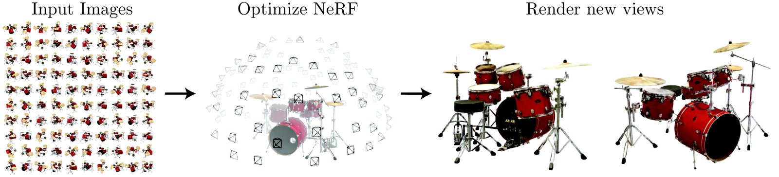
Figure 1: We present a method that optimizes a continuous 5D neural radiance field representation (volume density and view-dependent color at any continuous location) of a scene from a set of input images. We use techniques from volume rendering to accumulate samples of this scene representation along rays to render the scene from any viewpoint. Here, we visualize the set of 100 input views of the synthetic Drums scene randomly captured on a surrounding hemisphere, and we show two novel views rendered from our optimized NeRF representation.
图1:我们提出一种方法,从一组输入图像中优化一个场景的连续5D神经光度场代表(在任何连续位置的体积密度和视线依赖色). 我们利用体积渲染技术 沿着射线 积累这个场景的样本 在这里,我们将合成的Drums场景随机捕捉到的100个输入视图组合成影像,我们展现出从我们优化的NERF代表中得出的两个新视角.
Our approach inherits the benefits of volumetric representations: both can represent complex real-world geometry and appearance and are well suited for gradient-based optimization using projected images. Crucially, our method overcomes the prohibitive storage costs of discretized voxel grids when modeling complex scenes at high-resolutions. In summary, our technical contributions are:
我们的方法继承了量子表达的好处:既能代表复杂的现实世界几何和外观,又非常适合利用预测图像进行梯度优化. 关键是,当高分辨率模拟复杂场景时,我们的方法克服了“分散化的* voxel网格”的令人望而生畏的存储成本。 总之,我们的技术贡献是:
– An approach for representing continuous scenes with complex geometry and materials as 5D neural radiance fields, parameterized as basic MLP networks.
– A differentiable rendering procedure based on classical volume rendering techniques, which we use to optimize these representations from standard RGB images. This includes a hierarchical sampling strategy to allocate the MLP’s capacity towards space with visible scene content.
– A positional encoding to map each input 5D coordinate into a higher dimensional space, which enables us to successfully optimize neural radiance fields to represent high-frequency scene content.
——一种将具有复杂几何和材料的连续场景作为5D神经辐射场,参数化为基本MLP网络的方法.
– 一个基于古典量渲染技术的异质渲染程序,我们用它来优化这些表现与标准的RGB图像. 这包括一种分级取样战略,将MLP的能力分配给有可见场景内容的空间。
——定位编码,将每个输入5D坐标映射到一个更高的维空间,这使我们能够成功地优化神经辐射场,以代表高频场景内容.
We demonstrate that our resulting neural radiance field method quantitatively and qualitatively outperforms state-of-the-art view synthesis methods, including works that fit neural 3D representations to scenes as well as works that train deep convolutional networks to predict sampled volumetric representations. As far as we know, this paper presents the first continuous neural scene representation that is able to render high-resolution photorealistic novel views of real objects and scenes from RGB images captured in natural settings.
我们证明,我们由此产生的神经辐射场方法在数量和质量上都超过了最先进的视野合成方法,包括使神经3D表达与场景相适应的作品,以及训练深卷积网络以预测抽样的体积表达的作品。 据我们所知,本文呈现了第一个连续的神经场景表现,能够从自然环境下捕获的RGB图像中,对真实物体和场景进行高分辨率的光现实主义新视角.
2 Related Work
2 相关工作
A promising recent direction in computer vision is encoding objects and scenes in the weights of an MLP that directly maps from a 3D spatial location to an implicit representation of the shape, such as the signed distance [6] at that location. However, these methods have so far been unable to reproduce realistic scenes with complex geometry with the same fidelity as techniques that represent scenes using discrete representations such as triangle meshes or voxel grids. In this section, we review these two lines of work and contrast them with our approach, which enhances the capabilities of neural scene representations to produce state-of-the-art results for rendering complex realistic scenes.
计算机视觉中一个有希望的近期方向是将一个MLP的权重中的物体和场景编码,直接从3D空间位置映射到形状的隐含表现,如该位置的签名距离[6]. 然而,这些方法至今无法复制具有复杂几何特征的现实场景,与使用三角形网格或 voxel 网格等离散表示法代表场景的技术一样忠贞. 在本节中,我们回顾这两条工作线,并将其与我们的方法作对比,这提高了神经场景表现的能力,以产生最先进的结果,使复杂的现实场景.
A similar approach of using MLPs to map from low-dimensional coordinates to colors has also been used for representing other graphics functions such as images [44], textured materials [12, 31, 36, 37], and indirect illumination values [38].
使用MLP从低维坐标映射到颜色的类似方法也被用于代表其他图形函数,如图像[44],纹理材料[12,31,36,37],间接照明值[38].
Neural 3D shape representations
Recent work has investigated the implicit representation of continuous 3D shapes as level sets by optimizing deep networks that map coordinates to signed distance functions [15, 32] or occupancy fields [11, 27]. However, these models are limited by their requirement of access to ground truth 3D geometry, typically obtained from synthetic 3D shape datasets such as ShapeNet [3]. Subsequent work has relaxed this requirement of ground truth 3D shapes by formulating differentiable rendering functions that allow neural implicit shape representations to be optimized using only 2D images. Niemeyer et al. [29] represent surfaces as 3D occupancy fields and use a numerical method to find the surface intersection for each ray, then calculate an exact derivative using implicit differentiation. Each ray intersection location is provided as the input to a neural 3D texture field that predicts a diffuse color for that point. Sitzmann et al. [42] use a less direct neural 3D representation that simply outputs a feature vector and RGB color at each continuous 3D coordinate, and propose a differentiable rendering function consisting of a recurrent neural network that marches along each ray to decide where the surface is located.
神经3D形状表达式
最近的工作通过优化将坐标映射到签名的距离函数[15,32]或占用域[11,27]的深层网络,调查了连续立体形状作为水平集的隐含表现. 然而,这些模型受到其获取地面真言3D几何的要求的限制,这些三维几何通常是从合成3D形状数据集如ShapeNet[3]获得的. 随后的作品通过制定不同的渲染功能,使神经内含的形状表示能够仅使用2D图像进行优化,从而放宽了对地面真理3D形状的这一要求. Niemeyer *et *. [29] 代表表面为3D占用场,并使用数值法为每个射线寻找表面交叉点,然后使用隐含的区分计算出精确的衍生物. 每个射线交叉位置都作为神经3D纹理场的输入,预测该点的散色. Sitzmann *et *. [42] 使用一个不太直接的神经3D表示法,简单地在每个连续的3D坐标上输出一个特征矢量和RGB的颜色,并提议一个不同的渲染功能,由一条沿每个射线行进的神经网络组成,以决定表面的位置.
Though these techniques can potentially represent complicated and high-resolution geometry, they have so far been limited to simple shapes with low geometric complexity, resulting in oversmoothed renderings. We show that an alternate strategy of optimizing networks to encode 5D radiance fields (3D volumes with 2D view-dependent appearance) can represent higher-resolution geometry and appearance to render photorealistic novel views of complex scenes.
虽然这些技术可能代表复杂和高分辨率的几何学,但迄今为止它们仅限于几何复杂性低的简单形状,导致渲染过度. 我们显示,优化网络的另一种策略是编码5D光域(3D卷,视星等为2D)可以代表更高分辨率的几何和外观,使复杂场景的光现实主义新视角.
View synthesis and image-based rendering
Given a dense sampling of views, photorealistic novel views can be reconstructed by simple light field sample interpolation techniques [21, 5, 7]. For novel view synthesis with sparser view sampling, the computer vision and graphics communities have made significant progress by predicting traditional geometry and appearance representations from observed images. One popular class of approaches uses mesh-based representations of scenes with either diffuse [48] or view-dependent [2, 8, 49] appearance. Differentiable rasterizers [4, 10, 23, 25] or pathtracers [22, 30] can directly optimize mesh representations to reproduce a set of input images using gradient descent. However, gradient-based mesh optimization based on image reprojection is often difficult, likely because of local minima or poor conditioning of the loss landscape. Furthermore, this strategy requires a template mesh with fixed topology to be provided as an initialization before optimization [22], which is typically unavailable for unconstrained real-world scenes.
查看合成和基于图像的渲染
由于观点的采样密集,光现实主义的新视角可以通过简单的光场采样插图技术重建[21,5,7]. 对于带有较稀疏视图抽样的新视角合成,计算机视野和图形群落通过预测从观测到的图像中得出的传统几何和外观表现,取得了显著进展. 一个受欢迎的类方法采用网格化的场景表现方式,其外观要么是分散的[48],要么是视而不见的[2,8,49]。 可分化的光栅[4,10,23,25]或路径tracer[22,30]可以直接优化网格表示,利用梯度下降来复制一组输入图像. 然而,基于图像再投影的梯度网格优化往往很困难,可能是由于当地迷你或失落景观条件差. 此外,这一策略要求在优化[22]前提供具有固定地形的模板网格作为初始化,对于不受约束的现实世界场景,通常无法使用。
Another class of methods use volumetric representations to address the task of high-quality photorealistic view synthesis from a set of input RGB images. Volumetric approaches are able to realistically represent complex shapes and materials, are well-suited for gradient-based optimization, and tend to produce less visually distracting artifacts than mesh-based methods. Early volumetric approaches used observed images to directly color voxel grids [19, 40, 45]. More recently, several methods [9, 13, 17, 28, 33, 43, 46, 52] have used large datasets of multiple scenes to train deep networks that predict a sampled volumetric representation from a set of input images, and then use either alpha-compositing [34] or learned compositing along rays to render novel views at test time. Other works have optimized a combination of convolutional networks (CNNs) and sampled voxel grids for each specific scene, such that the CNN can compensate for discretization artifacts from low resolution voxel grids [41] or allow the predicted voxel grids to vary based on input time or animation controls [24]. While these volumetric techniques have achieved impressive results for novel view synthesis, their ability to scale to higher resolution imagery is fundamentally limited by poor time and space complexity due to their discrete sampling — rendering higher resolution images requires a finer sampling of 3D space. We circumvent this problem by instead encoding a continuous volume within the parameters of a deep fully-connected neural network, which not only produces significantly higher quality renderings than prior volumetric approaches, but also requires just a fraction of the storage cost of those sampled volumetric representations.
另一类方法使用量子表示法来解决一组输入RGB图像中高质量光现实主义视图合成的任务. 量子法能够现实地代表复杂的形状和材料,非常适合以梯度为基础的优化,并且往往比以网格为基础的方法产生较少的视觉分散力的文物. 早期的量学方法使用观测到的图像来直接涂色阴道网格[19,40,45]. 最近 为什么不使用[9,13,17,28,33,43,46,52] 多种场景的大型数据集来训练从一组输入图像中预测一个抽样的体积表示的深层网络,然后使用α-集成[34] 或沿射线学习混凝土在测试时渲染出新颖的视角. 其他作品则优化了各特定场景的卷积网络(CNN)组合,并采样了Voxel网格,因此CNN可以补偿低分辨率Voxel网格的盘状变质文物[41],或者允许预测的Voxel网格根据输入时间或动画控制变化[24]. 虽然这些量子技术在新视觉合成上取得了令人印象深刻的结果,但是由于它们的离散取样,其时间和空间复杂性差,因此其规模化到更高分辨率图像的能力受到根本限制——使分辨率更高的图像需要更细细的三维空间取样. 我们绕过这个问题,在深度全连通神经网络的参数内编码一个连续体积,这种神经网络不仅产生比以前体积方法高得多的质量渲染,而且只需要这些体积表征的一小部分存储成本。
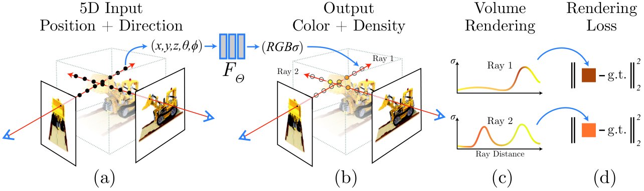
Figure 2: An overview of our neural radiance field scene representation and differentiable rendering procedure. We synthesize images by sampling 5D coordinates (location and viewing direction) along camera rays (a), feeding those locations into an MLP to produce a color and volume density (b), and using volume rendering techniques to composite these values into an image (c). This rendering function is differentiable, so we can optimize our scene representation by minimizing the residual between synthesized and ground truth observed images (d).
图2:我们神经光度场景表现和不同渲染程序的概述. 我们通过取样5D坐标(位置和视向)沿相机射线(a)合成图像,将这些位置输入MLP以产生颜色和体积密度(b),并利用体积渲染技术将这些值合成图像(c)。 这种渲染功能是不同的,因此我们可以通过将合成的和地面真实观测到的图像(d)之间的剩余部分降到最低,从而优化现场表现.
3 Neural Radiance Field Scene Representation
3 神经辐射场场景表示
We represent a continuous scene as a 5D vector-valued function whose input is a 3D location and 2D viewing direction , and whose output is an emitted color and volume density . In practice, we express direction as a 3D Cartesian unit vector . We approximate this continuous 5D scene representation with an MLP network and optimize its weights to map from each input 5D coordinate to its corresponding volume density and directional emitted color.
我们作为5D矢量值函数表示连续场景,其输入为3D位置和2D查看方向,其输出为释放色和体积密度. 在实践中,我们以3D笛卡尔单元矢量表示方向. 我们用一个 MLP 网络来估计这种连续的 5D 场景表现,并优化其的权重,从每个输入 5D 坐标到相应的体积密度和方向释放的颜色。
We encourage the representation to be multiview consistent by restricting the network to predict the volume density as a function of only the location , while allowing the RGB color to be predicted as a function of both location and viewing direction. To accomplish this, the MLP first processes the input 3D coordinate with 8 fully-connected layers (using ReLU activations and 256 channels per layer), and outputs and a 256-dimensional feature vector. This feature vector is then concatenated with the camera ray’s viewing direction and passed to one additional fully-connected layer (using a ReLU activation and 128 channels) that output the view-dependent RGB color.
我们鼓励通过限制网络预测体积密度仅作为位置的一种函数,同时允许预测RGB颜色同时作为位置和视图方向的一种函数,从而实现多视图一致. 为此,MLP 首先处理输入3D协调 与8个全连接层(使用ReLU激活和每层256通道),输出和一个256维特性矢量. 这个特性矢量随相机射线的视向而调和,然后传递到另外一个完全连接的层(使用ReLU激活和128通道),输出依赖视线的RGB颜色.
See Fig. 3 for an example of how our method uses the input viewing direction to represent non-Lambertian effects. As shown in Fig. 4, a model trained without view dependence (only as input) has difficulty representing specularities.
参见图3的一个例子,我们的方法如何使用输入查看方向来表示非兰伯特效应. 如图4所示,一个在不依赖视图的情况下训练的模型(只有作为输入)很难代表谱系.
4 Volume Rendering with Radiance Fields
4 辐射场的体积渲染
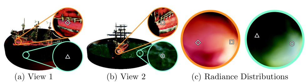
Figure 3: A visualization of view-dependent emitted radiance. Our neural radiance field representation outputs RGB color as a 5D function of both spatial position and viewing direction . Here, we visualize example directional color distributions for two spatial locations in our neural representation of the Ship scene. In (a) and (b), we show the appearance of two fixed 3D points from two different camera positions: one on the side of the ship (orange insets) and one on the surface of the water (blue insets). Our method predicts the changing specular appearance of these two 3D points, and in (c) we show how this behavior generalizes continuously across the whole hemisphere of viewing directions.
图3:视视视视视视视所释放的光线。 我们的神经光度场代表输出RGB颜色作为空间位置和查看方向的5D函数. 在这里,我们可视化两个空间位置的方向色分布 在我们的神经表现中,Ship场景。 在(a)和(b)中,我们从两个不同的相机位置显示两个固定的立体点的外观:一个位于舰体的侧面(橙色套),一个位于水面(蓝色套). 我们的方法预测了这两个三维点不断变化的光谱外观,在(c)中,我们显示了这种行为如何在整个半球持续地将视野方向概括起来.
Our 5D neural radiance field represents a scene as the volume density and directional emitted radiance at any point in space. We render the color of any ray passing through the scene using principles from classical volume rendering [16]. The volume density can be interpreted as the differential probability of a ray terminating at an infinitesimal particle at location . The expected color of camera ray with near and far bounds and is:
我们的5D神经辐射场 代表空间中任何一点的体积密度 和方向发射的辐射 我们利用古典体积渲染的原理 使任何射线穿过现场的颜色 [16]. 体积密度可以解释为在位置的无极粒子中射线终止的差分概率. 相机射线的预期颜色为 ,有近和远界和 :
C(\mathbf{r})=\int_{t_{n}}^{t_{f}}T(t)\sigma(\mathbf{r}(t))\mathbf{c}(\mathbf{r}(t),\mathbf{d})dt\,,\textrm{ where }T(t)=\exp\mathopen{}\mathclose{{\left(-\int_{t_{n}}^{t}\sigma(\mathbf{r}(s))ds}}\right)\,. \tag{1}
The function denotes the accumulated transmittance along the ray from to , i.e., the probability that the ray travels from to without hitting any other particle. Rendering a view from our continuous neural radiance field requires estimating this integral for a camera ray traced through each pixel of the desired virtual camera.
函数表示从到 , i. **.* 的射线沿射线的累积传导,即射线从到不撞击任何其他粒子的概率. 从我们连续的神经光度领域绘制一个视图,需要估计这个完整的,用于通过所期望的虚拟相机的每个像素追踪的相机射线.
We numerically estimate this continuous integral using quadrature. Deterministic quadrature, which is typically used for rendering discretized voxel grids, would effectively limit our representation’s resolution because the MLP would only be queried at a fixed discrete set of locations. Instead, we use a stratified sampling approach where we partition into evenly-spaced bins and then draw one sample uniformly at random from within each bin:
我们用四进制来估计这个连续的整体。 通常用于制作磁盘化的 voxel 网格的定型四进制会有效地限制我们代表的分辨率,因为MLP只会在一组固定的离散地点被询问。 相反,我们采用分层抽样方法,将分割为平方位的垃圾箱,然后从每个垃圾箱内随机抽取一个样本:
t_{i}\sim\mathcal{U}\mathopen{}\mathclose{{\left[t_{n}+\frac{i-1}{N}(t_{f}-t_{n}),\,\,t_{n}+\frac{i}{N}(t_{f}-t_{n})}}\right]\,. \tag{2}
Although we use a discrete set of samples to estimate the integral, stratified sampling enables us to represent a continuous scene representation because it results in the MLP being evaluated at continuous positions over the course of optimization. We use these samples to estimate with the quadrature rule discussed in the volume rendering review by Max [26]:
虽然我们使用一组离散的样品来估计整体的分层抽样,但使我们能够代表连续的场景表现,因为它导致在优化过程中在连续位置上对MLP进行评价。 我们用这些样本来估计, 并用Max [26] 在量渲染审查中讨论的四重规则:
\hat{C}(\mathbf{r})=\sum_{i=1}^{N}T_{i}(1-\exp\mathopen{}\mathclose{{\left(-\sigma_{i}\delta_{i}}}\right))\mathbf{c}_{i}\,,\textrm{ where }T_{i}=\exp\mathopen{}\mathclose{{\left(-\sum_{j=1}^{i-1}\sigma_{j}\delta_{j}}}\right)\,, \tag{3}
where is the distance between adjacent samples. This function for calculating from the set of values is trivially differentiable and reduces to traditional alpha compositing with alpha values \alpha_{i}=1-\exp\mathopen{}\mathclose{{\left(-\sigma_{i}\delta_{i}}}\right).
其中是相邻样本之间的距离。 计算从值集中算出的函数是微乎其微的,并缩小为传统的 α 堆肥 与 alpha 值\alpha_{i}=1-\exp\mathopen{}\mathclose{{\left(-\sigma_{i}\delta_{i}}}\right)。
5 Optimizing a Neural Radiance Field
5 优化神经辐射场
In the previous section we have described the core components necessary for modeling a scene as a neural radiance field and rendering novel views from this representation. However, we observe that these components are not sufficient for achieving state-of-the-art quality, as demonstrated in Section 6.4). We introduce two improvements to enable representing high-resolution complex scenes. The first is a positional encoding of the input coordinates that assists the MLP in representing high-frequency functions, and the second is a hierarchical sampling procedure that allows us to efficiently sample this high-frequency representation.
在上一节中,我们描述了将一个场景建模为神经光线场并从这一表述中提出新视角所必需的核心组成部分。 然而,我们注意到,这些组成部分不足以达到第6.4节所显示的最先进质量。 我们进行了两项改进,以便能够代表高分辨率的复杂场景。 第一个是协助MLP代表高频函数的输入坐标的位置编码,第二个是等级取样程序,使我们能够有效地取样这种高频表示。
| Ground Truth | Complete Model | No View Dependence | No Positional Encoding |
Figure 4: Here we visualize how our full model benefits from representing view-dependent emitted radiance and from passing our input coordinates through a high-frequency positional encoding. Removing view dependence prevents the model from recreating the specular reflection on the bulldozer tread. Removing the positional encoding drastically decreases the model’s ability to represent high frequency geometry and texture, resulting in an oversmoothed appearance.
| 事实 | 在联合国主持下, | 无视图依赖性 | 无位置编码 |
图4:我们可视化地看到,我们整个模型如何通过高频定位编码来表示视效辐射和传递输入坐标。 消除视图依赖性使得模型无法在推土机胎面上重新产生光谱反射. 移除位置编码会大幅降低模型代表高频几何和纹理的能力,导致外观过于平缓.
5.1 Positional encoding
5.1 位置编码
Despite the fact that neural networks are universal function approximators [14], we found that having the network directly operate on input coordinates results in renderings that perform poorly at representing high-frequency variation in color and geometry. This is consistent with recent work by Rahaman et al. [35], which shows that deep networks are biased towards learning lower frequency functions. They additionally show that mapping the inputs to a higher dimensional space using high frequency functions before passing them to the network enables better fitting of data that contains high frequency variation.
尽管神经网络是通用函数近似器[14],但我们发现,如果网络直接运行在输入坐标上,则渲染结果在表示颜色和几何高度的频率变化方面表现不佳. 这与拉哈曼(Rahaman *et *. [35])最近的工作是一致的,这说明深层网络偏向于学习低频功能. 它们进一步表明,利用高频函数将投入映射到更高维度空间后再传递到网络,可以更好地配置包含高频变化的数据。
We leverage these findings in the context of neural scene representations, and show that reformulating as a composition of two functions , one learned and one not, significantly improves performance (see Fig. 4 and Table 2). Here is a mapping from into a higher dimensional space , and is still simply a regular MLP. Formally, the encoding function we use is:
在神经场景表现方面,我们利用这些发现,并表明将重新编订为的两个功能,一个是学到的,另一个不是,大大提高了性能(见图4和表2)。 这里的是从绘制成一个更高的维空间的,而仍然只是一个普通的MLP. 在形式上,我们使用的编码功能是:
\gamma(p)=\mathopen{}\mathclose{{\left(\begin{array}[]{ccccc}\sin\mathopen{}\mathclose{{\left(2^{0}\pi p}}\right),&\cos\mathopen{}\mathclose{{\left(2^{0}\pi p}}\right),&\cdots,&\sin\mathopen{}\mathclose{{\left(2^{L-1}\pi p}}\right),&\cos\mathopen{}\mathclose{{\left(2^{L-1}\pi p}}\right)\end{array}}}\right)\,. \tag{4}
This function is applied separately to each of the three coordinate values in (which are normalized to lie in ) and to the three components of the Cartesian viewing direction unit vector (which by construction lie in ). In our experiments, we set for and for .
此函数分别应用于中的三个坐标值(它们通常位于)和笛卡尔视向单元矢量 的三个组件(通过构造存在于). 在我们的实验中,我们为设定了,为设定了.
A similar mapping is used in the popular Transformer architecture [47], where it is referred to as a positional encoding. However, Transformers use it for a different goal of providing the discrete positions of tokens in a sequence as input to an architecture that does not contain any notion of order. In contrast, we use these functions to map continuous input coordinates into a higher dimensional space to enable our MLP to more easily approximate a higher frequency function. Concurrent work on a related problem of modeling 3D protein structure from projections [51] also utilizes a similar input coordinate mapping.
在流行的Transformer架构中使用类似的映射[47],它被称为位置编码. 然而,Transformer使用它作为不同的目标,即以顺序提供符号的离散位置,作为对一个不包含任何秩序概念的架构的投入. 相比之下,我们利用这些功能将连续输入坐标映射到一个更高的维空间,使我们的MLP能够更容易地近似一个更高的频率函数. 同时在从预测中建模3D蛋白质结构的相关问题上开展的工作[51]也使用类似的输入坐标映射.
5.2 Hierarchical volume sampling
5.2 分层体积采样
Our rendering strategy of densely evaluating the neural radiance field network at query points along each camera ray is inefficient: free space and occluded regions that do not contribute to the rendered image are still sampled repeatedly. We draw inspiration from early work in volume rendering [20] and propose a hierarchical representation that increases rendering efficiency by allocating samples proportionally to their expected effect on the final rendering.
我们沿着每条相机射线的查询点对神经辐射场网络进行密集评价的渲染策略效率低下:对不促成成像的空闲空间和闭塞区域仍然反复取样. 我们从早期的量渲染[20]中汲取灵感,提出分级表述,通过按照样品对最终渲染的预期效果按比例分配样品来提高效率.
Instead of just using a single network to represent the scene, we simultaneously optimize two networks: one “coarse” and one “fine”. We first sample a set of locations using stratified sampling, and evaluate the “coarse” network at these locations as described in Eqns. 2 and 3. Given the output of this “coarse” network, we then produce a more informed sampling of points along each ray where samples are biased towards the relevant parts of the volume. To do this, we first rewrite the alpha composited color from the coarse network in Eqn. 3 as a weighted sum of all sampled colors along the ray:
我们不仅利用一个单一的网络来代表现场,而且还同时优化了两个网络:一个“粗”和一个“良好”。 我们首先利用分层抽样对一组地点进行抽样,并评估Eqns. 2和3所述这些地点的“粗”网络。 鉴于这一“粗体”网络的输出,我们然后对样品偏重于体积相关部分的每个射线沿线的点进行更知情的取样。 为此,我们首先将粗网在Eqn. 3中的α复合色重写为沿射线所有采样色的加权和:
\hat{C}_{c}(\mathbf{r})=\sum_{i=1}^{N_{c}}w_{i}c_{i}\,,\quad\,\,w_{i}=T_{i}(1-\exp\mathopen{}\mathclose{{\left(-\sigma_{i}\delta_{i}}}\right))\,. \tag{5}
Normalizing these weights as produces a piecewise-constant PDF along the ray. We sample a second set of locations from this distribution using inverse transform sampling, evaluate our “fine” network at the union of the first and second set of samples, and compute the final rendered color of the ray using Eqn. 3 but using all samples. This procedure allocates more samples to regions we expect to contain visible content. This addresses a similar goal as importance sampling, but we use the sampled values as a nonuniform discretization of the whole integration domain rather than treating each sample as an independent probabilistic estimate of the entire integral.
由于而使这些权重正常化,沿射线产生一个片式恒定PDF. 我们利用逆变取样从这种分布中抽取第二组地点,在第一和第二组样品结合时评价我们的“精良”网络,并使用Eqn. 3计算射线最后制成的颜色,但使用所有样品。 这一程序将更多的样本分配给我们希望含有可见内容的区域。 这涉及到一个与重要性取样相似的目标,但我们使用抽样的数值作为整个整合域的非统一盘点,而不是将每个样本作为整个整合域的独立概率估计.
5.3 Implementation details
5.3 实现细节
We optimize a separate neural continuous volume representation network for each scene. This requires only a dataset of captured RGB images of the scene, the corresponding camera poses and intrinsic parameters, and scene bounds (we use ground truth camera poses, intrinsics, and bounds for synthetic data, and use the COLMAP structure-from-motion package [39] to estimate these parameters for real data). At each optimization iteration, we randomly sample a batch of camera rays from the set of all pixels in the dataset, and then follow the hierarchical sampling described in Sec. 5.2 to query samples from the coarse network and samples from the fine network. We then use the volume rendering procedure described in Sec. 4 to render the color of each ray from both sets of samples. Our loss is simply the total squared error between the rendered and true pixel colors for both the coarse and fine renderings:
我们优化了每个场景的神经连续表达网络 这只需要一个数据集,其中包含被捕获的场景的RGB图像,相应的相机外观和内在参数,以及场景边框(我们使用地面真理相机外观,内在,边框来合成数据,并使用COLMAP结构-从动作包[39]来估计这些参数用于真实数据). 在每次优化迭代时,我们都会从数据集中所有像素的集合中随机抽取一批相机射线,然后按照Sec. 5 中描述的分级采样,查询粗细网络的X光和X光. 然后我们使用第4节中描述的体积渲染程序来制作出两组样本中每组射线的颜色。 我们的损失只是粗糙和细细的渲染 所呈现的像素颜色和真像素颜色之间的 完全方形错误:
\mathcal{L}=\sum_{\mathbf{r}\in\mathcal{R}}\mathopen{}\mathclose{{\left[\mathopen{}\mathclose{{\left\lVert\hat{C}_{c}(\mathbf{r})-C(\mathbf{r})}}\right\rVert_{2}^{2}+\mathopen{}\mathclose{{\left\lVert\hat{C}_{f}(\mathbf{r})-C(\mathbf{r})}}\right\rVert_{2}^{2}}}\right] \tag{6}
where is the set of rays in each batch, and , , and are the ground truth, coarse volume predicted, and fine volume predicted RGB colors for ray respectively. Note that even though the final rendering comes from , we also minimize the loss of so that the weight distribution from the coarse network can be used to allocate samples in the fine network.
其中是每批中的一组射线,而,和是地面真理,粗体积预测,细体积预测射线的RGB颜色. 注意,尽管最终渲染来自,但我们也将的损失降到最低,这样粗网的重量分布就可以用来在细网中分配样品.
In our experiments, we use a batch size of 4096 rays, each sampled at coordinates in the coarse volume and additional coordinates in the fine volume. We use the Adam optimizer [18] with a learning rate that begins at and decays exponentially to over the course of optimization (other Adam hyperparameters are left at default values of , , and ). The optimization for a single scene typically take around 100–300k iterations to converge on a single NVIDIA V100 GPU (about 1–2 days).
在我们的实验中,我们使用4096个射线的批量尺寸,每个样本在粗体积的坐标处采样,精体积的额外的坐标.所规定的义务,我们使用亚当优化器[18],学习率从开始,在优化过程中,衰减指数为(其他亚当超参数的默认值为,,和)。 单一场景的优化一般需要约100–300k的迭代才能在单一的NVIDIA V100 GPU上汇合(约1–2天).
6 Results
6 结果
We quantitatively (Tables 1) and qualitatively (Figs. 8 and 6) show that our method outperforms prior work, and provide extensive ablation studies to validate our design choices (Table 2). We urge the reader to view our supplementary video to better appreciate our method’s significant improvement over baseline methods when rendering smooth paths of novel views.
我们从数量(表1)和质量(图8和图6)来看,我们的方法比以前的工作要好,并提供了广泛的消化研究,以验证我们的设计选择(表2)。 我们促请读者观看我们的补充录像,
6.1 Datasets
6.1 数据集
Synthetic renderings of objects
We first show experimental results on two datasets of synthetic renderings of objects (Table 1, “Diffuse Synthetic ” and “Realistic Synthetic ”). The DeepVoxels [41] dataset contains four Lambertian objects with simple geometry. Each object is rendered at pixels from viewpoints sampled on the upper hemisphere (479 as input and 1000 for testing). We additionally generate our own dataset containing pathtraced images of eight objects that exhibit complicated geometry and realistic non-Lambertian materials. Six are rendered from viewpoints sampled on the upper hemisphere, and two are rendered from viewpoints sampled on a full sphere. We render 100 views of each scene as input and 200 for testing, all at pixels.
- 物体合成渲染
的三个天体合成渲染数据集(表1,“Diffuse Synthetic ”和“Realistic Synthetic ”)的实验结果。 DeepVoxels [41] 数据集包含四个具有简单几何特征的兰伯特天体. 每个物体在像素中从上半球取样的视点(479作为输入,1000作为测试)得到. 我们另外生成我们自己的数据集 包含8个物体的路径跟踪图像 显示复杂的几何和现实的非兰伯特材料。 六个来自上半球取样的观点,两个来自整个领域取样的观点。 我们给每个场景提供100个视图作为输入,200个用于测试,全部在像素.
| Ship | |||||
|---|---|---|---|---|---|
| Lego | |||||
| Microphone | |||||
| Materials | |||||
| Ground Truth | NeRF (ours) | LLFF [28] | SRN [42] | NV [24] |
Figure 5: Comparisons on test-set views for scenes from our new synthetic dataset generated with a physically-based renderer. Our method is able to recover fine details in both geometry and appearance, such as Ship’s rigging, Lego’s gear and treads, Microphone’s shiny stand and mesh grille, and Material’s non-Lambertian reflectance. LLFF exhibits banding artifacts on the Microphone stand and Material’s object edges and ghosting artifacts in Ship’s mast and inside the Lego object. SRN produces blurry and distorted renderings in every case. Neural Volumes cannot capture the details on the Microphone’s grille or Lego’s gears, and it completely fails to recover the geometry of Ship’s rigging.
| 飞船 | |||||
|---|---|---|---|---|---|
| 莱戈 | |||||
| 麦克风 | |||||
| 材料 | |||||
| 事实 | 新的或新的 | LLFF [28] (法语). | SRN [42] (英语). | NV [24] (英语). |
图5:用物理渲染器生成的我们新的合成数据集的场景的测试集视图比较。 我们的方法能够恢复几何和外观上的细微细节,例如: Ship’s raping, Lego’s 齿轮和脚印, Microphone’s 闪亮的立体和网状烤架,以及 Matrial’s 非兰伯特式反射。 LLFF展品在 麦克风展台和 Matrial’s的物体边缘上以及 Ship’s桅杆和 Lego物体内部的幽灵文物。 SRN在每一个案件中都会产生模糊和扭曲的渲染. 神经卷无法捕捉到 *麦克风的烤箱或 Lego’s齿轮上的细节,完全无法恢复 Ship’s rogging的几何特征.
Real images of complex scenes
We show results on complex real-world scenes captured with roughly forward-facing images (Table 1, “Real Forward-Facing”). This dataset consists of 8 scenes captured with a handheld cellphone (5 taken from the LLFF paper and 3 that we capture), captured with 20 to 62 images, and hold out of these for the test set. All images are pixels.
复杂场景的真实图像
我们用大致向前看的图像(表1,“真实向前看”)来展示复杂的现实世界场景的结果。 这个数据集包括8个用手持手机捕获的场景(5个取自LLFF纸,3个取自我们所捕获的),用20到62个图像捕获的场景,并将其中的用于测试集. 所有图像均为像素.
| Fern | ||||
|---|---|---|---|---|
| T-Rex | ||||
| Orchid | ||||
| Ground Truth | NeRF (ours) | LLFF [28] | SRN [42] |
Figure 6: Comparisons on test-set views of real world scenes. LLFF is specifically designed for this use case (forward-facing captures of real scenes). Our method is able to represent fine geometry more consistently across rendered views than LLFF, as shown in Fern’s leaves and the skeleton ribs and railing in T-rex. Our method also correctly reconstructs partially occluded regions that LLFF struggles to render cleanly, such as the yellow shelves behind the leaves in the bottom Fern crop and green leaves in the background of the bottom Orchid crop. Blending between multiples renderings can also cause repeated edges in LLFF, as seen in the top Orchid crop. SRN captures the low-frequency geometry and color variation in each scene but is unable to reproduce any fine detail.
| 芬兰 | ||||
|---|---|---|---|---|
| T-Rex (英语). | ||||
| 兰花 | ||||
| 事实 | NERF( 我们) | LLFF [28] (法语). | SRN [42] (英语). |
图6:真实世界场景测试集视图比较. LLFF是专门为这个使用案例设计的(前向的拍摄真实场景). 我们的方法能够比 LLFF 更连贯地 表达出精细的几何特征, 我们 我们的方法也正确地重建了部分占有的LLFF努力使土地变得干净的区域,例如底部的叶子后面的黄色架子Fern作物和底部的绿叶兰花作物的背景. 多重渲染之间的混合也可以在LLFF中引起重复的边缘,如顶部的兰花作物. SRN捕捉到每个场景中的低频几何和颜色变化,但无法复制任何细微的细节.
| Diffuse Synthetic [41] | Realistic Synthetic | Real Forward-Facing [28] | |||||||
|---|---|---|---|---|---|---|---|---|---|
| Method | PSNR | SSIM | LPIPS | PSNR | SSIM | LPIPS | PSNR | SSIM | LPIPS |
| SRN [42] | |||||||||
| NV [24] | - | - | - | ||||||
| LLFF [28] | |||||||||
| Ours |
Table 1: Our method quantitatively outperforms prior work on datasets of both synthetic and real images. We report PSNR/SSIM (higher is better) and LPIPS [50] (lower is better). The DeepVoxels [41] dataset consists of 4 diffuse objects with simple geometry. Our realistic synthetic dataset consists of pathtraced renderings of 8 geometrically complex objects with complex non-Lambertian materials. The real dataset consists of handheld forward-facing captures of 8 real-world scenes (NV cannot be evaluated on this data because it only reconstructs objects inside a bounded volume). Though LLFF achieves slightly better LPIPS, we urge readers to view our supplementary video where our method achieves better multiview consistency and produces fewer artifacts than all baselines.
| 阐释合成[41] | 现实合成 | 真正的前方阵容姻缘[28] | |||||||
|---|---|---|---|---|---|---|---|---|---|
| 方法 | 二十届理事会第一期会议 | SSIM 二十届理事会 | LPIPS(英语). | 二十届理事会第一期会议 | SSIM 二十届理事会 | LPIPS(英语). | 二十届理事会第一期会议 | SSIM 二十届理事会 | LPIPS(英语). |
| SRN [42] (英语). | |||||||||
| NV [24] (英语). | - | - | - | ||||||
| LLFF [28] (法语). | |||||||||
| 我们的 |
表1:我们的方法在数量上超过了以前在合成和真实图像数据集方面的工作。 我们报告PSNR/SSIM(较高更好)和LPIPS50。 DeepVoxels [41] 数据集由4个具有简单几何特征的分散天体组成. 我们的现实合成数据集由8个几何复杂物体的路径跟踪渲染组成,具有复杂的非兰伯特材料. 真正的数据集包括手持式前立式抓取8个现实世界场景(NV不能在此数据上评价,因为它只重建一个有界量内的物体). 虽然LLFF的LPIPS成绩稍好,但我们敦促读者观看我们的补充视频,我们的方法可以实现更好的多视图一致性,并生产比所有基线更少的文物。
6.2 Comparisons
6.2 对比实验
To evaluate our model we compare against current top-performing techniques for view synthesis, detailed below. All methods use the same set of input views to train a separate network for each scene except Local Light Field Fusion [28], which trains a single 3D convolutional network on a large dataset, then uses the same trained network to process input images of new scenes at test time.
为了评价我们的模型,我们比较了目前最高性能的视图综合技术,详情如下。 所有方法都使用相同的一组输入视图来为每个场景训练一个单独的网络,除了Local Light Field Fusion[28],它在一个大型数据集上训练一个单一的3D卷积网络,然后使用同样的训练有素的网络在测试时处理新场景的输入图像.
Neural Volumes (NV) [24]
synthesizes novel views of objects that lie entirely within a bounded volume in front of a distinct background (which must be separately captured without the object of interest). It optimizes a deep 3D convolutional network to predict a discretized RGB voxel grid with samples as well as a 3D warp grid with samples. The algorithm renders novel views by marching camera rays through the warped voxel grid.
** 神经卷(NV)** [24]
综合了完全位于一个特定背景(必须单独捕捉,而不包含感兴趣的对象)前的限定卷内的物体的新视角. 它优化了深3D卷积网络,以预测带有样本的盘状RGBvoxel网格以及带有样本的3D曲速网格. 该算法通过将相机射线通过扭曲的voxel网格来进行新颖的视图.
Scene Representation Networks (SRN) [42]
represent a continuous scene as an opaque surface, implicitly defined by a MLP that maps each coordinate to a feature vector. They train a recurrent neural network to march along a ray through the scene representation by using the feature vector at any 3D coordinate to predict the next step size along the ray. The feature vector from the final step is decoded into a single color for that point on the surface. Note that SRN is a better-performing followup to DeepVoxels [41] by the same authors, which is why we do not include comparisons to DeepVoxels.
** 现场代表网(SRN)** [42]
代表连续场景作为不透明的表面,由MLP暗含定义,将每个坐标映射到特征矢量. 他们通过在任何3D坐标上使用特征矢量来预测沿射线的下一步大小,来训练一个反复出现的神经网络,沿着射线穿过场景代表线行进. 最后一步的特征矢量被解码为表面该点的单一颜色. 注意,SRN是同一作者对DeepVoxels[41]的更好表现的后续,这就是为什么我们不包含与DeepVoxels的比较.
Local Light Field Fusion (LLFF) [28]
LLFF is designed for producing photorealistic novel views for well-sampled forward facing scenes. It uses a trained 3D convolutional network to directly predict a discretized frustum-sampled RGB grid (multiplane image or MPI [52]) for each input view, then renders novel views by alpha compositing and blending nearby MPIs into the novel viewpoint.
** 当地轻型场融合(LLFF)** [28]
LLFF是用来制作摄影现实主义小说观点,用于对前方的面景进行很好的取样. 它使用训练有素的3D卷积网络,直接预测每个输入视图的盘状浮雕样本RGB 网格(多飞机图像或MPI [52]),然后通过α堆肥和将附近的MPI混合到新视角中来制作新视角.
6.3 Discussion
6.3 讨论
We thoroughly outperform both baselines that also optimize a separate network per scene (NV and SRN) in all scenarios. Furthermore, we produce qualitatively and quantitatively superior renderings compared to LLFF (across all except one metric) while using only their input images as our entire training set.
我们完全超越了两个基线,这些基线还优化了每个场景的单独网络(NV和SRN)。 此外,我们 如果你不使用他们输入的图像作为整个培训集,则会制作质量和数量上的优于LLFF的图像。
The SRN method produces heavily smoothed geometry and texture, and its representational power for view synthesis is limited by selecting only a single depth and color per camera ray. The NV baseline is able to capture reasonably detailed volumetric geometry and appearance, but its use of an underlying explicit voxel grid prevents it from scaling to represent fine details at high resolutions. LLFF specifically provides a “sampling guideline” to not exceed 64 pixels of disparity between input views, so it frequently fails to estimate correct geometry in the synthetic datasets which contain up to 400-500 pixels of disparity between views. Additionally, LLFF blends between different scene representations for rendering different views, resulting in perceptually-distracting inconsistency as is apparent in our supplementary video.
SRN方法产生高度平滑的几何和纹理,其用于视图合成的表示力由于每个相机射线只选择一个单一的深度和颜色而受到限制. NV基线能够捕捉到合理详细的体积几何和外观,但是它使用一个基础明确的 voxel网格使其无法缩放在高分辨率上代表细细的细节. LLFF专门提供了一个“抽样指南”,不超过输入视图之间差异的64像素,因此它常常无法估计合成数据集中正确几何,其中包含最多400-500像素的视图之间差异。 此外,LLFF将不同场景的表述混为一谈,以表达不同的观点,从而造成我们补充视频中明显可见的洞察力分散的不一致。
The biggest practical tradeoffs between these methods are time versus space. All compared single scene methods take at least 12 hours to train per scene. In contrast, LLFF can process a small input dataset in under 10 minutes. However, LLFF produces a large 3D voxel grid for every input image, resulting in enormous storage requirements (over 15GB for one “Realistic Synthetic” scene). Our method requires only 5 MB for the network weights (a relative compression of compared to LLFF), which is even less memory than the input images alone for a single scene from any of our datasets.
这些方法之间最大的实际权衡是时间与空间。 所有比较的单一场景方法至少需要12小时来训练每个场景. 相比之下,LLFF可以在不到10分钟内处理一个小的输入数据集. 然而,LLFF为每个输入图像生成一个大的3D voxel网格,导致巨大的存储要求(一个"真实合成"场景超过15GB). 我们的方法只需要网络权重的5 MB(与 LLFF 相比,相对压缩), 其内存甚至比 * 输入图像单独 * 对于我们任何一个数据集的单个场景都更少.
6.4 Ablation studies
6.4 消融实验
| Input | #Im. | PSNR | SSIM | LPIPS | ||||
|---|---|---|---|---|---|---|---|---|
| 1) | No PE, VD, H | 100 | - | (256, - ) | ||||
| 2) | No Pos. Encoding | 100 | - | (64, 128) | ||||
| 3) | No View Dependence | 100 | 10 | (64, 128) | ||||
| 4) | No Hierarchical | 100 | 10 | (256, - ) | ||||
| 5) | Far Fewer Images | 25 | 10 | (64, 128) | ||||
| 6) | Fewer Images | 50 | 10 | (64, 128) | ||||
| 7) | Fewer Frequencies | 100 | 5 | (64, 128) | ||||
| 8) | More Frequencies | 100 | 15 | (64, 128) | ||||
| 9) | Complete Model | 100 | 10 | (64, 128) |
Table 2: An ablation study of our model. Metrics are averaged over the 8 scenes from our realistic synthetic dataset. See Sec. 6.4 for detailed descriptions.
| 投入 | {\fn方正粗倩简体\fs12\an8\1cHFFFF00\b0}我 | 二十届理事会第一期会议 | SSIM 二十届理事会 | LPIPS(英语). | ||||
|---|---|---|---|---|---|---|---|---|
| 1) | 无PE、VD、H | 100 | - | (256, - ) | ||||
| 2) | 无 Pos 编码 | 第二十届 | 100 | - | (64, 128) | |||
| 3) | 无视图依赖性 | 100 | 10 | (64, 128) | ||||
| 4) | 无等级 | 二十负责处理 | 100 | 10 | (256, - ) | |||
| 5) | 远小图像 | 第二十届 | 25 | 10 | (64, 128) | |||
| 6) | 减少图像 | 第二十届 | 50 | 10 | (64, 128) | |||
| 7) | 频率减少 | 第二十届 | 100 | 5 | (64, 128) | |||
| 8) | 更多细节 | 第二十届 | 100 | 15 | (64, 128) | |||
| 9) | 完整模型 | 第二十届 | 100 | 10 | (64, 128) |
表2:关于我们模式的研究。 从我们现实的合成数据集中 平均有8个场景 详细描述见第6.4节。
We validate our algorithm’s design choices and parameters with an extensive ablation study in Table 2. We present results on our “Realistic Synthetic ” scenes. Row 9 shows our complete model as a point of reference. Row 1 shows a minimalist version of our model without positional encoding (PE), view-dependence (VD), or hierarchical sampling (H). In rows 2–4 we remove these three components one at a time from the full model, observing that positional encoding (row 2) and view-dependence (row 3) provide the largest quantitative benefit followed by hierarchical sampling (row 4). Rows 5–6 show how our performance decreases as the number of input images is reduced. Note that our method’s performance using only 25 input images still exceeds NV, SRN, and LLFF across all metrics when they are provided with 100 images (see supplementary material). In rows 7–8 we validate our choice of the maximum frequency used in our positional encoding for (the maximum frequency used for is scaled proportionally). Only using 5 frequencies reduces performance, but increasing the number of frequencies from 10 to 15 does not improve performance. We believe the benefit of increasing is limited once exceeds the maximum frequency present in the sampled input images (roughly 1024 in our data).
我们通过表2中的一项广泛的衰减研究来验证我们算法的设计选择和参数。 我们介绍了我们“真实合成”场景的结果。 第9行显示了我们完整的模型作为参照点. 第1行显示我们的模型的最小化版本,没有位置编码(PE),视图依赖(VD),或等级抽样(H). 在第2至第4行中,我们将这三部分从整个模型中逐一删除,观察位置编码(第2行)和视距依赖(第3行)提供了最大的定量效益,其次是等级抽样(第4行)。 第5-6行显示,随着输入图像数量的减少,我们的性能会如何下降。 请注意,当我们的方法仅使用25个输入图像时,其性能仍然超过NV、SRN和LLFF,在提供100个图像时(见补充材料)。 在第7至第8行中,我们验证了我们在定位编码中使用的最大频率的选择(所使用的最大频率按比例缩放)。 只有使用5个频率才能降低性能,但将频率从10个增加到15个并不能改善性能. 我们认为,一旦超过抽样输入图像中的最大频率(我们的数据大约为1024),增加的好处就会受到限制。
7 Conclusion
7 结论
Our work directly addresses deficiencies of prior work that uses MLPs to represent objects and scenes as continuous functions. We demonstrate that representing scenes as 5D neural radiance fields (an MLP that outputs volume density and view-dependent emitted radiance as a function of 3D location and 2D viewing direction) produces better renderings than the previously-dominant approach of training deep convolutional networks to output discretized voxel representations.
我们的工作直接解决了前作中使用MLP作为连续函数来表示对象和场景的缺陷. 我们证明,将场景作为5D神经辐射场(一种通过3D定位和2D视向来输出体积密度和视光发射的光度的MLP),所产生的渲染效果优于以往培训深卷积网络以输出光碟化的阴道表示法。
Although we have proposed a hierarchical sampling strategy to make rendering more sample-efficient (for both training and testing), there is still much more progress to be made in investigating techniques to efficiently optimize and render neural radiance fields. Another direction for future work is interpretability: sampled representations such as voxel grids and meshes admit reasoning about the expected quality of rendered views and failure modes, but it is unclear how to analyze these issues when we encode scenes in the weights of a deep neural network. We believe that this work makes progress towards a graphics pipeline based on real world imagery, where complex scenes could be composed of neural radiance fields optimized from images of actual objects and scenes.
虽然我们提出了一个分级取样战略,以提高采样效率(用于培训和测试),但在有效优化和使神经辐射场化的调查技术方面仍有许多进展。 未来工作的另一个方向是可解释性:被抽样的表示,如voxel网格和meshes,承认了对所渲染的视图和故障模式的预期质量的推理,但当我们在深层神经网络的权重中编码场景时尚不清楚如何分析这些问题. 我们认为,这项工作在建立基于真实世界图像的图形管道方面取得了进展,其中复杂的场景可以由从实际物体和场景的图像中优化出来的神经光场组成。
Acknowledgements We thank Kevin Cao, Guowei Frank Yang, and Nithin Raghavan for comments and discussions. RR acknowledges funding from ONR grants N000141712687 and N000142012529 and the Ronald L. Graham Chair. BM is funded by a Hertz Foundation Fellowship, and MT is funded by an NSF Graduate Fellowship. Google provided a generous donation of cloud compute credits through the BAIR Commons program. We thank the following Blend Swap users for the models used in our realistic synthetic dataset: gregzaal (ship), 1DInc (chair), bryanajones (drums), Herberhold (ficus), erickfree (hotdog), Heinzelnisse (lego), elbrujodelatribu (materials), and up3d.de (mic).
** 承认** 我们感谢曹凯文、郭伟、杨弗兰克和尼辛·拉哈万的发言和讨论。 RR确认来自ONR赠款N000141712687和N000142012529以及Ronald L.Graham主席的资助。 BM由赫兹基金会研究金资助,MT由NSF研究生研究金资助. Google通过BAIR Communitys计划慷慨捐赠云计算信用. 我们感谢下列Blend Swap用户在我们现实的合成数据集中使用的模型:gregzaal(飞船)、1Dinc(主席)、bryanajones(鼓),Herberhold(ficus),erickfree(hotdog),Heinzelnisse(lego),elbrujodelatribu(材料)和 up3d.de(mic)。
References
参考文献
[1] Abadi, M., Agarwal, A., Barham, P., Brevdo, E., Chen, Z., Citro, C., Corrado, G.S., Davis, A., Dean, J., Devin, M., Ghemawat, S., Goodfellow, I., Harp, A., Irving, G., Isard, M., Jia, Y., Jozefowicz, R., Kaiser, L., Kudlur, M., Levenberg, J., Mané, D., Monga, R., Moore, S., Murray, D., Olah, C., Schuster, M., Shlens, J., Steiner, B., Sutskever, I., Talwar, K., Tucker, P., Vanhoucke, V., Vasudevan, V., Viégas, F., Vinyals, O., Warden, P., Wattenberg, M., Wicke, M., Yu, Y., Zheng, X.: TensorFlow: Large-scale machine learning on heterogeneous systems (2015)
[2] Buehler, C., Bosse, M., McMillan, L., Gortler, S., Cohen, M.: Unstructured lumigraph rendering. In: SIGGRAPH (2001)
[3] Chang, A.X., Funkhouser, T., Guibas, L., Hanrahan, P., Huang, Q., Li, Z., Savarese, S., Savva, M., Song, S., Su, H., et al.: Shapenet: An information-rich 3d model repository. arXiv:1512.03012 (2015)
[4] Chen, W., Gao, J., Ling, H., Smith, E.J., Lehtinen, J., Jacobson, A., Fidler, S.: Learning to predict 3D objects with an interpolation-based differentiable renderer. In: NeurIPS (2019)
[5] Cohen, M., Gortler, S.J., Szeliski, R., Grzeszczuk, R., Szeliski, R.: The lumigraph. In: SIGGRAPH (1996)
[6] Curless, B., Levoy, M.: A volumetric method for building complex models from range images. In: SIGGRAPH (1996)
[7] Davis, A., Levoy, M., Durand, F.: Unstructured light fields. In: Eurographics (2012)
[8] Debevec, P., Taylor, C.J., Malik, J.: Modeling and rendering architecture from photographs: A hybrid geometry-and image-based approach. In: SIGGRAPH (1996)
[9] Flynn, J., Broxton, M., Debevec, P., DuVall, M., Fyffe, G., Overbeck, R., Snavely, N., Tucker, R.: DeepView: view synthesis with learned gradient descent. In: CVPR (2019)
[10] Genova, K., Cole, F., Maschinot, A., Sarna, A., Vlasic, D., , Freeman, W.T.: Unsupervised training for 3D morphable model regression. In: CVPR (2018)
[11] Genova, K., Cole, F., Sud, A., Sarna, A., Funkhouser, T.: Local deep implicit functions for 3d shape. In: CVPR (2020)
[12] Henzler, P., Mitra, N.J., Ritschel, T.: Learning a neural 3d texture space from 2d exemplars. In: CVPR (2020)
[13] Henzler, P., Rasche, V., Ropinski, T., Ritschel, T.: Single-image tomography: 3d volumes from 2d cranial x-rays. In: Eurographics (2018)
[14] Hornik, K., Stinchcombe, M., White, H.: Multilayer feedforward networks are universal approximators. Neural Networks (1989)
[15] Jiang, C., Sud, A., Makadia, A., Huang, J., Nießner, M., Funkhouser, T.: Local implicit grid representations for 3d scenes. In: CVPR (2020)
[16] Kajiya, J.T., Herzen, B.P.V.: Ray tracing volume densities. Computer Graphics (SIGGRAPH) (1984)
[17] Kar, A., Häne, C., Malik, J.: Learning a multi-view stereo machine. In: NeurIPS (2017)
[18] Kingma, D.P., Ba, J.: Adam: A method for stochastic optimization. In: ICLR (2015)
[19] Kutulakos, K.N., Seitz, S.M.: A theory of shape by space carving. International Journal of Computer Vision (2000)
[20] Levoy, M.: Efficient ray tracing of volume data. ACM Transactions on Graphics (1990)
[21] Levoy, M., Hanrahan, P.: Light field rendering. In: SIGGRAPH (1996)
[22] Li, T.M., Aittala, M., Durand, F., Lehtinen, J.: Differentiable monte carlo ray tracing through edge sampling. ACM Transactions on Graphics (SIGGRAPH Asia) (2018)
[23] Liu, S., Li, T., Chen, W., Li, H.: Soft rasterizer: A differentiable renderer for image-based 3D reasoning. In: ICCV (2019)
[24] Lombardi, S., Simon, T., Saragih, J., Schwartz, G., Lehrmann, A., Sheikh, Y.: Neural volumes: Learning dynamic renderable volumes from images. ACM Transactions on Graphics (SIGGRAPH) (2019)
[25] Loper, M.M., Black, M.J.: OpenDR: An approximate differentiable renderer. In: ECCV (2014)
[26] Max, N.: Optical models for direct volume rendering. IEEE Transactions on Visualization and Computer Graphics (1995)
[27] Mescheder, L., Oechsle, M., Niemeyer, M., Nowozin, S., Geiger, A.: Occupancy networks: Learning 3D reconstruction in function space. In: CVPR (2019)
[28] Mildenhall, B., Srinivasan, P.P., Ortiz-Cayon, R., Kalantari, N.K., Ramamoorthi, R., Ng, R., Kar, A.: Local light field fusion: Practical view synthesis with prescriptive sampling guidelines. ACM Transactions on Graphics (SIGGRAPH) (2019)
[29] Niemeyer, M., Mescheder, L., Oechsle, M., Geiger, A.: Differentiable volumetric rendering: Learning implicit 3D representations without 3D supervision. In: CVPR (2019)
[30] Nimier-David, M., Vicini, D., Zeltner, T., Jakob, W.: Mitsuba 2: A retargetable forward and inverse renderer. ACM Transactions on Graphics (SIGGRAPH Asia) (2019)
[31] Oechsle, M., Mescheder, L., Niemeyer, M., Strauss, T., Geiger, A.: Texture fields: Learning texture representations in function space. In: ICCV (2019)
[32] Park, J.J., Florence, P., Straub, J., Newcombe, R., Lovegrove, S.: DeepSDF: Learning continuous signed distance functions for shape representation. In: CVPR (2019)
[33] Penner, E., Zhang, L.: Soft 3D reconstruction for view synthesis. ACM Transactions on Graphics (SIGGRAPH Asia) (2017)
[34] Porter, T., Duff, T.: Compositing digital images. Computer Graphics (SIGGRAPH) (1984)
[35] Rahaman, N., Baratin, A., Arpit, D., Dräxler, F., Lin, M., Hamprecht, F.A., Bengio, Y., Courville, A.C.: On the spectral bias of neural networks. In: ICML (2018)
[36] Rainer, G., Ghosh, A., Jakob, W., Weyrich, T.: Unified neural encoding of BTFs. Computer Graphics Forum (Eurographics) (2020)
[37] Rainer, G., Jakob, W., Ghosh, A., Weyrich, T.: Neural BTF compression and interpolation. Computer Graphics Forum (Eurographics) (2019)
[38] Ren, P., Wang, J., Gong, M., Lin, S., Tong, X., Guo, B.: Global illumination with radiance regression functions. ACM Transactions on Graphics (2013)
[39] Schönberger, J.L., Frahm, J.M.: Structure-from-motion revisited. In: CVPR (2016)
[40] Seitz, S.M., Dyer, C.R.: Photorealistic scene reconstruction by voxel coloring. International Journal of Computer Vision (1999)
[41] Sitzmann, V., Thies, J., Heide, F., Nießner, M., Wetzstein, G., Zollhöfer, M.: Deepvoxels: Learning persistent 3D feature embeddings. In: CVPR (2019)
[42] Sitzmann, V., Zollhoefer, M., Wetzstein, G.: Scene representation networks: Continuous 3D-structure-aware neural scene representations. In: NeurIPS (2019)
[43] Srinivasan, P.P., Tucker, R., Barron, J.T., Ramamoorthi, R., Ng, R., Snavely, N.: Pushing the boundaries of view extrapolation with multiplane images. In: CVPR (2019)
[44] Stanley, K.O.: Compositional pattern producing networks: A novel abstraction of development. Genetic programming and evolvable machines (2007)
[45] Szeliski, R., Golland, P.: Stereo matching with transparency and matting. In: ICCV (1998)
[46] Tulsiani, S., Zhou, T., Efros, A.A., Malik, J.: Multi-view supervision for single-view reconstruction via differentiable ray consistency. In: CVPR (2017)
[47] Vaswani, A., Shazeer, N., Parmar, N., Uszkoreit, J., Jones, L., Gomez, A.N., Kaiser, Ł., Polosukhin, I.: Attention is all you need. In: NeurIPS (2017)
[48] Waechter, M., Moehrle, N., Goesele, M.: Let there be color! Large-scale texturing of 3D reconstructions. In: ECCV (2014)
[49] Wood, D.N., Azuma, D.I., Aldinger, K., Curless, B., Duchamp, T., Salesin, D.H., Stuetzle, W.: Surface light fields for 3D photography. In: SIGGRAPH (2000)
[50] Zhang, R., Isola, P., Efros, A.A., Shechtman, E., Wang, O.: The unreasonable effectiveness of deep features as a perceptual metric. In: CVPR (2018)
[51] Zhong, E.D., Bepler, T., Davis, J.H., Berger, B.: Reconstructing continuous distributions of 3D protein structure from cryo-EM images. In: ICLR (2020)
[52] Zhou, T., Tucker, R., Flynn, J., Fyffe, G., Snavely, N.: Stereo magnification: Learning view synthesis using multiplane images. ACM Transactions on Graphics (SIGGRAPH) (2018)
Appendix 0.A Additional Implementation Details
附录 0.A 额外实现细节
Network Architecture
Fig. 7 details our simple fully-connected architecture.
网络结构
图7详细介绍了我们简单的全连接建筑.
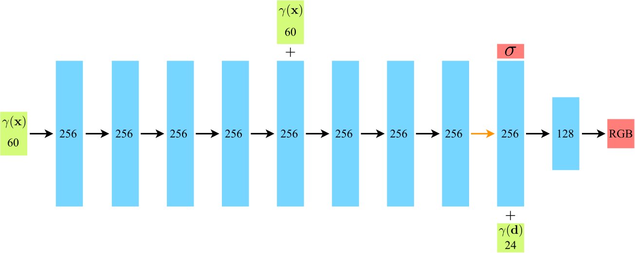
Figure 7: A visualization of our fully-connected network architecture. Input vectors are shown in green, intermediate hidden layers are shown in blue, output vectors are shown in red, and the number inside each block signifies the vector’s dimension. All layers are standard fully-connected layers, black arrows indicate layers with ReLU activations, orange arrows indicate layers with no activation, dashed black arrows indicate layers with sigmoid activation, and “+” denotes vector concatenation. The positional encoding of the input location () is passed through 8 fully-connected ReLU layers, each with 256 channels. We follow the DeepSDF [32] architecture and include a skip connection that concatenates this input to the fifth layer’s activation. An additional layer outputs the volume density (which is rectified using a ReLU to ensure that the output volume density is nonnegative) and a 256-dimensional feature vector. This feature vector is concatenated with the positional encoding of the input viewing direction (), and is processed by an additional fully-connected ReLU layer with 128 channels. A final layer (with a sigmoid activation) outputs the emitted RGB radiance at position , as viewed by a ray with direction .
图7:我们全联网网络架构的可视化. 输入矢量以绿色显示,中间隐藏层以蓝色显示,输出矢量以红色显示,每个块内的数字表示矢量的维度. 所有层都是标准的全连接层,黑色箭头表示带有ReLU激活的层,橙色箭头表示没有激活的层,破折黑箭头表示带有sigmoid激活的层,"+"表示矢量凝聚. 输入位置()的位置编码通过8个全连接的ReLU层传递,每个层有256个信道. 我们遵循 DeepSDF [32] 架构, 并包含一个跳过连接, 另一层输出体积密度(使用ReLU进行修正,以确保输出体积密度非负式)和256维特性矢量。 此特性矢量与输入查看方向()的位置编码相配合,由额外的全连接的ReLU层与128通道进行处理. 最后一层(带有Sigmoid激活)在位置输出发射的RGB光度,由带有方向的射线查看。
Volume Bounds
Our method renders views by querying the neural radiance field representation at continuous 5D coordinates along camera rays. For experiments with synthetic images, we scale the scene so that it lies within a cube of side length 2 centered at the origin, and only query the representation within this bounding volume. Our dataset of real images contains content that can exist anywhere between the closest point and infinity, so we use normalized device coordinates to map the depth range of these points into . This shifts all the ray origins to the near plane of the scene, maps the perspective rays of the camera to parallel rays in the transformed volume, and uses disparity (inverse depth) instead of metric depth, so all coordinates are now bounded.
音量边界
我们的方法通过在相机射线沿线的连续5D坐标上查询神经光度的场面代表来表达观点. 对于合成图像的实验,我们放大了场景,使它位于一个以原物为中心的侧长2的立方体内,并且只查询在这个边长体积内的表示. 我们真实图像的数据集包含了可以存在于最近点和无限点之间的任何地方的内容,因此我们使用常态化的设备坐标将这些点的深度范围映射到. 这把所有的射线起源都转移到了场景的近平面上,将相机的视角射线映射到变形体积中的平行射线上,并使用差异(反深度)而不是度量深度,所以现在所有的坐标都被定界了.
Training Details
For real scene data, we regularize our network by adding random Gaussian noise with zero mean and unit variance to the output values (before passing them through the ReLU) during optimization, finding that this slightly improves visual performance for rendering novel views. We implement our model in Tensorflow [1].
培训详情
对于真实的场景数据,我们通过在优化期间将零平均值和单位差异的随机高斯噪音加入输出值(在通过ReLU传递之前)来规范我们的网络,发现这稍稍改进了渲染新颖视图的视觉性能. 我们在Tensorflow执行我们的模型[1].
Rendering Details
To render new views at test time, we sample points per ray through the coarse network and points per ray through the fine network, for a total of network queries per ray. Our realistic synthetic dataset requires 640k rays per image, and our real scenes require 762k rays per image, resulting in between 150 and 200 million network queries per rendered image. On an NVIDIA V100, this takes approximately 30 seconds per frame.
编译细节
为了在试验时提出新的观点,我们通过粗网对每条射线的点进行抽样,通过细网对每条射线的点进行抽样,总共为每条射线的网络查询. 我们的现实合成数据集每张图像需要640k射线,我们真实的场景每张图像需要762k射线,结果每张渲染的图像需要1.5亿到2亿个网络查询. 在NVIDIA V100上,每帧大约需要30秒.
Appendix 0.B Additional Baseline Method Details
附录 0.B 额外基线方法细节
Neural Volumes (NV) [24]
We use the NV code open-sourced by the authors at https://github.com/facebookresearch/neuralvolumes and follow their procedure for training on a single scene without time dependence.
** 神经卷(NV)** [24]
我们使用作者在https://github.com/facebookresearch/neural voles上开源的NV代码,并遵循他们在一个单一场景上训练的程序,而不依赖时间.
Scene Representation Networks (SRN) [42]
We use the SRN code open-sourced by the authors at https://github.com/vsitzmann/scene-representation-networks and follow their procedure for training on a single scene.
** 现场代表网(SRN)** [42]
我们使用作者在https://github.com/vsitzmann/scene-presentation-network上开源的SRN代码,并遵循他们在单一场景上的培训程序.
Local Light Field Fusion (LLFF) [28]
We use the pretrained LLFF model open-sourced by the authors at https://github.com/Fyusion/LLFF.
** 当地轻型场融合(LLFF)** [28]
Quantitative Comparisons
The SRN implementation published by the authors requires a significant amount of GPU memory, and is limited to an image resolution of pixels even when parallelized across 4 NVIDIA V100 GPUs. We compute quantitative metrics for SRN at pixels for our synthetic datasets and pixels for the real datasets, in comparison to and respectively for the other methods that can be run at higher resolutions.
定量比较
作者发布的 SRN 执行需要大量GPU内存,并且被限制在像素的图像分辨率上,即使平行于4个NVIDIA V100 GPU. 我们计算用于合成数据集的SRN在像素上的定量度量衡,用于真实数据集的像素则分别计算用于以更高分辨率运行的其他方法的和.
Appendix 0.C NDC ray space derivation
附录 0.C NDC 射线空间推导
We reconstruct real scenes with “forward facing” captures in the normalized device coordinate (NDC) space that is commonly used as part of the triangle rasterization pipeline. This space is convenient because it preserves parallel lines while converting the axis (camera axis) to be linear in disparity.
我们重建真正的场景,在通常用作三角光栅化管道一部分的常态设备坐标空间中“前向”捕捉。 这种空间是方便的,因为它在将轴(相机轴)转换为线性差异时保留平行线.
Here we derive the transformation which is applied to rays to map them from camera space to NDC space. The standard 3D perspective projection matrix for homogeneous coordinates is:
在这里,我们得出了应用在射线上的变换,从相机空间将其映射到NDC空间. 同一坐标的标准三维视角投影矩阵是:
$$M=\begin{pmatrix}\frac{n}{r}&0&0&0\
0&\frac{n}{t}&0&0\
0&0&\frac{-(f+n)}{f-n}&\frac{-2fn}{f-n}\
0&0&-1&0\end{pmatrix} \tag{7}$$
where are the near and far clipping planes and and are the right and top bounds of the scene at the near clipping plane. (Note that this is in the convention where the camera is looking in the direction.) To project a homogeneous point , we left-multiply by M and then divide by the fourth coordinate:
其中是近和远的剪报飞机,和是近剪报飞机上场景的左右界限. (注意这是相机向方向看的公约. ) 为了投射一个同位点,我们左乘M,然后用第四个坐标:
$$\displaystyle\begin{pmatrix}\frac{n}{r}&0&0&0\
0&\frac{n}{t}&0&0\
0&0&\frac{-(f+n)}{f-n}&\frac{-2fn}{f-n}\
0&0&-1&0\end{pmatrix}\begin{pmatrix}x\
y\
z\
1\end{pmatrix} \ \displaystyle=\begin{pmatrix}\frac{n}{r}x\
\frac{n}{t}y\
\frac{-(f+n)}{f-n}z-\frac{-2fn}{f-n}\
-z\end{pmatrix} \ \displaystyle\rightarrow\begin{pmatrix}\frac{n}{r}\frac{x}{-z}\
\frac{n}{t}\frac{y}{-z}\
\frac{(f+n)}{f-n}-\frac{2fn}{f-n}\frac{1}{-z}\end{pmatrix} \tag{8}$$
The projected point is now in normalized device coordinate (NDC) space, where the original viewing frustum has been mapped to the cube .
投影点现在处于正态设备坐标空间(NDC)中,这里的原始查看浮图已经映射到立方体.
Our goal is to take a ray and calculate a ray origin and direction in NDC space such that for every , there exists a new for which (where is projection using the above matrix). In other words, the projection of the original ray and the NDC space ray trace out the same points (but not necessarily at the same rate).
我们的目标是取射线并在NDC空间中计算射线源和方向,这样每就有一个新的,其中(使用上述矩阵预测). 换句话说,原始射线和NDC空间射线的投射会追踪到相同的点(但不一定以相同的速度).
Let us rewrite the projected point from Eqn. 9 as . The components of the new origin and direction must satisfy:
让我们从Eqn.9重写预测点为。 新来源和方向的组件必须满足:
$$\displaystyle\begin{pmatrix}a_{x}\frac{o_{x}+td_{x}}{o_{z}+td_{z}}\[6.0pt]
a_{y}\frac{o_{y}+td_{y}}{o_{z}+td_{z}}\[6.0pt]
a_{z}+\frac{b_{z}}{o_{z}+td_{z}}\end{pmatrix}=\begin{pmatrix}o_{x}^{\prime}+t^{\prime}d_{x}^{\prime}\
o_{y}^{\prime}+t^{\prime}d_{y}^{\prime}\
o_{z}^{\prime}+t^{\prime}d_{z}^{\prime}\end{pmatrix},. \tag{10}$$
To eliminate a degree of freedom, we decide that and should map to the same point. Substituting and Eqn. 10 directly gives our NDC space origin :
为了消除一定程度的自由,我们决定,和应绘制到同一点. 替换和 Eqn. 10直接给了我们的NDC空间源:
$$\displaystyle\mathbf{o}^{\prime}=\begin{pmatrix}o_{x}^{\prime}\
o_{y}^{\prime}\
o_{z}^{\prime}\end{pmatrix}=\begin{pmatrix}a_{x}\frac{o_{x}}{o_{z}}\[6.0pt]
a_{y}\frac{o_{y}}{o_{z}}\[6.0pt]
a_{z}+\frac{b_{z}}{o_{z}}\end{pmatrix}=\pi(\mathbf{o}),. \tag{11}$$
This is exactly the projection of the original ray’s origin. By substituting this back into Eqn. 10 for arbitrary , we can determine the values of and :
这恰恰是原射线源的投影. 将它替换为 Eqn. 10 来表示任意的 , 我们可以确定和的值 :
$$\displaystyle\begin{pmatrix}t^{\prime}d_{x}^{\prime}\
t^{\prime}d_{y}^{\prime}\
t^{\prime}d_{z}^{\prime}\end{pmatrix} \ \displaystyle=\begin{pmatrix}a_{x}\frac{o_{x}+td_{x}}{o_{z}+td_{z}}-a_{x}\frac{o_{x}}{o_{z}}\[6.0pt]
a_{y}\frac{o_{y}+td_{y}}{o_{z}+td_{z}}-a_{y}\frac{o_{y}}{o_{z}}\[6.0pt]
a_{z}+\frac{b_{z}}{o_{z}+td_{z}}-a_{z}-\frac{b_{z}}{o_{z}}\end{pmatrix} \ \displaystyle=\begin{pmatrix}a_{x}\frac{o_{z}(o_{x}+td_{x})-o_{x}(o_{z}+td_{z})}{(o_{z}+td_{z})o_{z}}\[6.0pt]
a_{y}\frac{o_{z}(o_{y}+td_{y})-o_{y}(o_{z}+td_{z})}{(o_{z}+td_{z})o_{z}}\[6.0pt]
b_{z}\frac{o_{z}-(o_{z}+td_{z})}{(o_{z}+td_{z})o_{z}}\end{pmatrix} \ \displaystyle=\begin{pmatrix}a_{x}\frac{td_{z}}{o_{z}+td_{z}}\mathopen{}\mathclose{{\left(\frac{d_{x}}{d_{z}}-\frac{o_{x}}{o_{z}}}}\right)\[6.0pt]
a_{y}\frac{td_{z}}{o_{z}+td_{z}}\mathopen{}\mathclose{{\left(\frac{d_{y}}{d_{z}}-\frac{o_{y}}{o_{z}}}}\right)\[6.0pt]
-b_{z}\frac{td_{z}}{o_{z}+td_{z}}\frac{1}{o_{z}}\end{pmatrix} \tag{12}$$
Factoring out a common expression that depends only on gives us:
考虑一个仅依赖于的常用表达式给我们:
$$\displaystyle t^{\prime} \ \displaystyle=\frac{td_{z}}{o_{z}+td_{z}}=1-\frac{o_{z}}{o_{z}+td_{z}} \ \displaystyle\mathbf{d}^{\prime} \ \displaystyle=\begin{pmatrix}a_{x}\mathopen{}\mathclose{{\left(\frac{d_{x}}{d_{z}}-\frac{o_{x}}{o_{z}}}}\right)\[6.0pt]
a_{y}\mathopen{}\mathclose{{\left(\frac{d_{y}}{d_{z}}-\frac{o_{y}}{o_{z}}}}\right)\[6.0pt]
-b_{z}\frac{1}{o_{z}}\end{pmatrix},. \tag{15}$$
Note that, as desired, when . Additionally, we see that as . Going back to the original projection matrix, our constants are:
请注意,如所希望,在. 此外,我们将第号视为第号。 回到原来的投影矩阵,我们的常数是:
Using the standard pinhole camera model, we can reparameterize as:
使用标准的针孔相机模型,我们可以重新校准如下:
where and are the width and height of the image in pixels and is the focal length of the camera.
其中和是图像在像素中的宽度和高度,是相机的焦距.
In our real forward facing captures, we assume that the far scene bound is infinity (this costs us very little since NDC uses the dimension to represent inverse depth, i.e., disparity). In this limit the constants simplify to:
在我们面对捕捉的真正前进中,我们假设,远处的场景是无限的(由于NDC使用维度来代表反深度,即差异,这使我们付出的代价很小)。 在这个限制中,常数简化为:
Combining everything together:
将一切结合起来:
$$\displaystyle\mathbf{o}^{\prime} \ \displaystyle=\begin{pmatrix}-\frac{f_{cam}}{W/2}\frac{o_{x}}{o_{z}}\[6.0pt]
-\frac{f_{cam}}{H/2}\frac{o_{y}}{o_{z}}\[6.0pt]
1+\frac{2n}{o_{z}}\end{pmatrix} \ \displaystyle\mathbf{d}^{\prime} \ \displaystyle=\begin{pmatrix}-\frac{f_{cam}}{W/2}\mathopen{}\mathclose{{\left(\frac{d_{x}}{d_{z}}-\frac{o_{x}}{o_{z}}}}\right)\[6.0pt]
-\frac{f_{cam}}{H/2}\mathopen{}\mathclose{{\left(\frac{d_{y}}{d_{z}}-\frac{o_{y}}{o_{z}}}}\right)\[6.0pt]
-2n\frac{1}{o_{z}}\end{pmatrix},. \tag{25}$$
One final detail in our implementation: we shift to the ray’s intersection with the near plane at (before this NDC conversion) by taking for . Once we convert to the NDC ray, this allows us to simply sample linearly from to in order to get a linear sampling in disparity from to in the original space.
我们实施中的最后一点细节是:我们把移到(这次NDC转换之前)的射线与近平面的交叉点,取作为. 一旦我们转换成NDC射线,我们就可以简单地从到线性地取样,以便在原空间从到的差异中获得线性取样.
Appendix 0.D Additional Results
附录 0.D 额外结果
Per-scene breakdown
Tables 3, 4, 5, and 6 include a breakdown of the quantitative results presented in the main paper into per-scene metrics. The per-scene breakdown is consistent with the aggregate quantitative metrics presented in the paper, where our method quantitatively outperforms all baselines. Although LLFF achieves slightly better LPIPS metrics, we urge readers to view our supplementary video where our method achieves better multiview consistency and produces fewer artifacts than all baselines.
- 场面破损
表3、4、5和6将主要文件中提出的量化结果细分为每个场面的衡量标准。 每一场面的细分与文件中提出的总的量化度量一致,我们的方法在数量上超过了所有基线。 尽管LLFF的LPIPS衡量标准稍有改进,但我们敦促读者观看我们的补充视频,我们的方法在其中实现更好的多视图一致性,并生产比所有基线更少的文物。
| Pedestal | |||||
|---|---|---|---|---|---|
| Cube | |||||
| Ground Truth | NeRF (ours) | LLFF [28] | SRN [42] | NV [24] |
Figure 8: Comparisons on test-set views for scenes from the DeepVoxels [41] synthetic dataset. The objects in this dataset have simple geometry and perfectly diffuse reflectance. Because of the large number of input images (479 views) and simplicity of the rendered objects, both our method and LLFF [28] perform nearly perfectly on this data. LLFF still occasionally presents artifacts when interpolating between its 3D volumes, as in the top inset for each object. SRN [42] and NV [24] do not have the representational power to render fine details.
| 履历 | |||||
|---|---|---|---|---|---|
| * 立方体 * | |||||
| 事实 | NERF( 我们) | LLFF [28] (法语). | SRN [42] (英语). | NV [24] (英语). |
图8:DeepVoxels的场景测试集视图比较[41]合成数据集. 这个数据集中的物体具有简单的几何和完全分散的反射. 由于大量输入图像(479视图)以及渲染对象的简单化,我们的方法和LLFF[28]都在这个数据上几乎完美地表现. LLFF在其3D卷间插图时仍然偶尔会呈现文物,如每个物体的顶部插图. SRN[42]和NV[24]没有代表权力提供细微的细节.
| PSNR | SSIM | LPIPS | ||||||||||
|---|---|---|---|---|---|---|---|---|---|---|---|---|
| Chair | Pedestal | Cube | Vase | Chair | Pedestal | Cube | Vase | Chair | Pedestal | Cube | Vase | |
| DeepVoxels [41] | ||||||||||||
| SRN [42] | ||||||||||||
| NV [24] | ||||||||||||
| LLFF [28] | ||||||||||||
| Ours |
Table 3: Per-scene quantitative results from the DeepVoxels [41] dataset. The “scenes” in this dataset are all diffuse objects with simple geometry, rendered from texture-mapped meshes captured by a 3D scanner. The metrics for the DeepVoxels method are taken directly from their paper, which does not report LPIPS and only reports two significant figures for SSIM.
| 二十届理事会第一期会议 | SSIM 二十届理事会 | LPIPS(英语). | ||||||||||
|---|---|---|---|---|---|---|---|---|---|---|---|---|
| 页:1 | 台词 | 立方体 | 宽度 | 页:1 | 台词 | 立方体 | 宽度 | 页:1 | 台词 | 立方体 | 宽度 | |
| 你不该说 | ||||||||||||
| SRN [42] (英语). | ||||||||||||
| NV [24] (英语). | ||||||||||||
| LLFF [28] (法语). | ||||||||||||
| 我们的 |
表3:深福克斯数据集的人均场面定量结果[41]. 本数据集中的“场景 我要你用3D扫描仪捕获的纹理映射的薄膜制成的简单几何物体。 DeepVoxels方法的度量衡直接取自他们的论文,该论文不报告LPIPS,只报告SSIM的两个重要数字.
| PSNR | ||||||||
|---|---|---|---|---|---|---|---|---|
| Chair | Drums | Ficus | Hotdog | Lego | Materials | Mic | Ship | |
| SRN [42] | ||||||||
| NV [24] | ||||||||
| LLFF [28] | ||||||||
| Ours |
| SSIM | ||||||||
|---|---|---|---|---|---|---|---|---|
| Chair | Drums | Ficus | Hotdog | Lego | Materials | Mic | Ship | |
| SRN [42] | ||||||||
| NV [24] | ||||||||
| LLFF [28] | ||||||||
| Ours |
| LPIPS | ||||||||
|---|---|---|---|---|---|---|---|---|
| Chair | Drums | Ficus | Hotdog | Lego | Materials | Mic | Ship | |
| SRN [42] | ||||||||
| NV [24] | ||||||||
| LLFF [28] | ||||||||
| Ours |
Table 4: Per-scene quantitative results from our realistic synthetic dataset. The “scenes” in this dataset are all objects with more complex gometry and non-Lambertian materials, rendered using Blender’s Cycles pathtracer.
| 二十届理事会第一期会议 | ||||||||
|---|---|---|---|---|---|---|---|---|
| 页:1 | 鼓声 | 菲克斯语Name | 热狗 | 乐高 | 材料 | 麦可 | 船舶 | |
| 69. 斯洛伐克[42] | ||||||||
| NV [24] (英语). | ||||||||
| LLFF [28] (法语). | ||||||||
| 我们的 |
| SSIM 二十届理事会 | ||||||||
|---|---|---|---|---|---|---|---|---|
| 页:1 | 这是鼓声 | 菲克斯语Name | 热狗 | 乐高 | 材料 | 麦可 | 船舶 | |
| SRN [42] (英语). | ||||||||
| NV [24] (英语). | ||||||||
| LLFF [28] (法语). | ||||||||
| 我们的 |
| LPIPS(英语). | ||||||||
|---|---|---|---|---|---|---|---|---|
| 页:1 | 鼓声 | 菲克斯语Name | 热狗 | 乐高 | 材料 | 麦可 | 船舶 | |
| SRN [42] (英语). | ||||||||
| NV [24] (英语). | ||||||||
| LLFF [28] (法语). | ||||||||
| 我们的 |
表4:我国现实合成数据集的人均场面定量结果. 本数据集中的 " 场景 " 是指使用Blender的循环径向器制成的具有更复杂的直径测量和非Lambertian材料的所有物体。
| PSNR | ||||||||
|---|---|---|---|---|---|---|---|---|
| Room | Fern | Leaves | Fortress | Orchids | Flower | T-Rex | Horns | |
| SRN [42] | ||||||||
| LLFF [28] | ||||||||
| Ours |
| SSIM | ||||||||
|---|---|---|---|---|---|---|---|---|
| Room | Fern | Leaves | Fortress | Orchids | Flower | T-Rex | Horns | |
| SRN [42] | ||||||||
| LLFF [28] | ||||||||
| Ours |
| LPIPS | ||||||||
|---|---|---|---|---|---|---|---|---|
| Room | Fern | Leaves | Fortress | Orchids | Flower | T-Rex | Horns | |
| SRN [42] | ||||||||
| LLFF [28] | ||||||||
| Ours |
Table 5: Per-scene quantitative results from our real image dataset. The scenes in this dataset are all captured with a forward-facing handheld cellphone.
| 二十届理事会第一期会议 | ||||||||
|---|---|---|---|---|---|---|---|---|
| 会议室 | 费恩 | 叶子 | 堡垒 | 奥 让 | 鲜花 | T- Rex 调色器 | 喇叭 | |
| SRN [42] (英语). | ||||||||
| LLFF [28] (法语). | ||||||||
| 我们的 |
| SSIM 二十届理事会 | ||||||||
|---|---|---|---|---|---|---|---|---|
| 会议室 | 费恩 | 叶子 | 堡垒 | 兰花 | 鲜花 | T- Rex 调色器 | 喇叭 | |
| SRN [42] (英语). | ||||||||
| LLFF [ Moorem] [28] (法语). | ||||||||
| 我们的 |
| LPIPS(英语). | ||||||||
|---|---|---|---|---|---|---|---|---|
| 会议室 | 费恩 | 叶子 | 堡垒 | 兰花 | 鲜花 | T- Rex 调色器 | 喇叭 | |
| SRN [42] (英语). | ||||||||
| LLFF [28] (法语). | ||||||||
| 我们的 |
表5:我们真实的图像数据集得出的人均数量结果。 1920 scenes được captured captured captured set set
| PSNR | |||||||||
|---|---|---|---|---|---|---|---|---|---|
| Chair | Drums | Ficus | Hotdog | Lego | Materials | Mic | Ship | ||
| 1) | No PE, VD, H | ||||||||
| 2) | No Pos. Encoding | ||||||||
| 3) | No View Dependence | ||||||||
| 4) | No Hierarchical | ||||||||
| 5) | Far Fewer Images | ||||||||
| 6) | Fewer Images | ||||||||
| 7) | Fewer Frequencies | ||||||||
| 8) | More Frequencies | ||||||||
| 9) | Complete Model |
| SSIM | |||||||||
|---|---|---|---|---|---|---|---|---|---|
| Chair | Drums | Ficus | Hotdog | Lego | Materials | Mic | Ship | ||
| 1) | No PE, VD, H | ||||||||
| 2) | No Pos. Encoding | ||||||||
| 3) | No View Dependence | ||||||||
| 4) | No Hierarchical | ||||||||
| 5) | Far Fewer Images | ||||||||
| 6) | Fewer Images | ||||||||
| 7) | Fewer Frequencies | ||||||||
| 8) | More Frequencies | ||||||||
| 9) | Complete Model |
| LPIPS | |||||||||
|---|---|---|---|---|---|---|---|---|---|
| Chair | Drums | Ficus | Hotdog | Lego | Materials | Mic | Ship | ||
| 1) | No PE, VD, H | ||||||||
| 2) | No Pos. Encoding | ||||||||
| 3) | No View Dependence | ||||||||
| 4) | No Hierarchical | ||||||||
| 5) | Far Fewer Images | ||||||||
| 6) | Fewer Images | ||||||||
| 7) | Fewer Frequencies | ||||||||
| 8) | More Frequencies | ||||||||
| 9) | Complete Model |
Table 6: Per-scene quantitative results from our ablation study. The scenes used here are the same as in Table 4.
| PhiladelphianR数据 | |||||||||
|---|---|---|---|---|---|---|---|---|---|
| 页:1 | 鼓声 | 菲克斯语Name | 热狗 | 乐高 | 材料 | 麦可 | 船舶 | ||
| 1) | 无PE、VD、H | ||||||||
| 2) | 无 Pos 编码 | ||||||||
| 3) | 无视图依赖性 | ||||||||
| 4) | 无等级 | ||||||||
| 5) | 远小图像 | ||||||||
| 6) | 减少图像 | ||||||||
| 7) | 更 是的 少 点 | ||||||||
| 8) | 更多细节 | ||||||||
| 9) | 完整模型 |
| SSIM 二十届理事会 | |||||||||
|---|---|---|---|---|---|---|---|---|---|
| 页:1 | Dr | 菲克斯语Name | 热狗 | 乐高 | 材料 | 麦可 | 船舶 | ||
| 1) | 无PE、VD、H | ||||||||
| 2) | 无 Pos 编码 | ||||||||
| 3) | 无视图依赖性 | ||||||||
| 4) | 遵从等级 | ||||||||
| 5) | 远小图像 | ||||||||
| 6) | 减少图像 | ||||||||
| 7) | 频率减少 | ||||||||
| 8) | 更多细节 | ||||||||
| 9) | 方面的活动 |
| 你想说什么? | |||||||||
|---|---|---|---|---|---|---|---|---|---|
| 页:1 | 鼓声 | 协商会 | 热狗 | 乐高 | 材料 | 米克昵称 | 船舶 | ||
| 1) | 无PE、VD、H | ||||||||
| 2) | 无 Pos 编码 | ||||||||
| 3) | 无视图依赖性 | ||||||||
| 4) | 无等级 | ||||||||
| 5) | 远小图像 | ||||||||
| 6) | 减少图像 | ||||||||
| 7) | 频率减少 | ||||||||
| 8) | 更多细节 | ||||||||
| 9) | 完整模型 |
表6:我国消化研究得出的人均场面定量结果. 这里使用的场景与表4相同.