Mastering Atari, Go, Chess and Shogi by Planning with a Learned Model
Mastering Atari, Go, Chess and Shogi by Planning with a Learned Model
用学得的模型做规划,通关 Atari、围棋、国际象棋与将棋
Julian Schrittwieser Ioannis Antonoglou Thomas Hubert Affiliation: DeepMind, 6 Pancras Square, London N1C 4AG. Karen Simonyan Laurent Sifre Affiliation: DeepMind, 6 Pancras Square, London N1C 4AG. Simon Schmitt Affiliation: DeepMind, 6 Pancras Square, London N1C 4AG. Arthur Guez Affiliation: DeepMind, 6 Pancras Square, London N1C 4AG. Edward Lockhart Demis Hassabis Affiliation: DeepMind, 6 Pancras Square, London N1C 4AG. Thore Graepel Affiliation: DeepMind, 6 Pancras Square, London N1C 4AG. Timothy Lillicrap Affiliation: DeepMind, 6 Pancras Square, London N1C 4AG. Affiliation: University College London, Gower Street, London WC1E 6BT. ∗ These authors contributed equally to this work. David Silver Affiliation: DeepMind, 6 Pancras Square, London N1C 4AG.
Abstract
摘要
Constructing agents with planning capabilities has long been one of the main challenges in the pursuit of artificial intelligence. Tree-based planning methods have enjoyed huge success in challenging domains, such as chess and Go, where a perfect simulator is available. However, in real-world problems the dynamics governing the environment are often complex and unknown. In this work we present the MuZero algorithm which, by combining a tree-based search with a learned model, achieves superhuman performance in a range of challenging and visually complex domains, without any knowledge of their underlying dynamics. MuZero learns a model that, when applied iteratively, predicts the quantities most directly relevant to planning: the reward, the action-selection policy, and the value function. When evaluated on 57 different Atari games - the canonical video game environment for testing AI techniques, in which model-based planning approaches have historically struggled - our new algorithm achieved a new state of the art. When evaluated on Go, chess and shogi, without any knowledge of the game rules, MuZero matched the superhuman performance of the AlphaZero algorithm that was supplied with the game rules.
让智能体具备规划能力,一直是人工智能的核心难题之一。在象棋、围棋这类有完美模拟器的领域,基于树搜索的规划已取得巨大成功;但现实问题中,环境动力学往往复杂且未知。本文提出 MuZero:把树搜索与学得的模型结合起来,在多种挑战性、视觉复杂的领域达到超人类水平,且无需任何底层动力学先验。MuZero 学到的模型经迭代应用后,直接预测对规划最相关的量:奖励、动作选择策略与价值函数。在 57 款 Atari 游戏——检验 AI 技术的经典视频游戏环境,模型规划方法此前一直吃力——新算法刷新了当时最优结果。在围棋、国际象棋与将棋上,即便完全不知规则,MuZero 也达到了配有规则信息的 AlphaZero 的超人类表现。
1 Introduction
1 引言
Planning algorithms based on lookahead search have achieved remarkable successes in artificial intelligence. Human world champions have been defeated in classic games such as checkers [34], chess [5], Go [38] and poker [3, 26], and planning algorithms have had real-world impact in applications from logistics [47] to chemical synthesis [37]. However, these planning algorithms all rely on knowledge of the environment’s dynamics, such as the rules of the game or an accurate simulator, preventing their direct application to real-world domains like robotics, industrial control, or intelligent assistants.
基于前瞻搜索的规划算法在人工智能中取得了显著成功。人类世界冠军已在跳棋 [34]、国际象棋 [5]、围棋 [38] 与扑克 [3, 26] 等经典博弈中被击败;规划算法也在物流 [47] 到化学合成 [37] 等现实应用中产生影响。但这些算法都依赖对环境动力学的知识——例如游戏规则或精确模拟器——因而无法直接用于机器人、工业控制或智能助手等真实场景。
Model-based reinforcement learning (RL) [42] aims to address this issue by first learning a model of the environment’s dynamics, and then planning with respect to the learned model. Typically, these models have either focused on reconstructing the true environmental state [8, 16, 24], or the sequence of full observations [14, 20]. However, prior work [4, 14, 20] remains far from the state of the art in visually rich domains, such as Atari 2600 games [2]. Instead, the most successful methods are based on model-free RL [9, 21, 18] – i.e. they estimate the optimal policy and/or value function directly from interactions with the environment. However, model-free algorithms are in turn far from the state of the art in domains that require precise and sophisticated lookahead, such as chess and Go.
基于模型的强化学习(RL)[42] 试图先学环境动力学模型,再在学得的模型上规划。这类模型通常聚焦于重建真实环境状态 [8, 16, 24],或完整观测序列 [14, 20]。但先前工作 [4, 14, 20] 在 Atari 2600 [2] 这类视觉丰富领域仍远落后于当时最优。最成功的方法反而来自无模型 RL [9, 21, 18]——即直接从与环境的交互中估计最优策略和/或价值函数。反过来,无模型算法在象棋、围棋等需要精确、精细前瞻的领域又远落后于当时最优。
In this paper, we introduce MuZero, a new approach to model-based RL that achieves state-of-the-art performance in Atari 2600, a visually complex set of domains, while maintaining superhuman performance in precision planning tasks such as chess, shogi and Go. MuZero builds upon AlphaZero’s [39] powerful search and search-based policy iteration algorithms, but incorporates a learned model into the training procedure. MuZero also extends AlphaZero to a broader set of environments including single agent domains and non-zero rewards at intermediate time-steps.
本文提出 MuZero:一种新的基于模型的 RL 方法,在视觉复杂的 Atari 2600 上达到当时最优,同时在国际象棋、将棋与围棋等精确规划任务上保持超人类水平。MuZero 建立在 AlphaZero [39] 强大的搜索与基于搜索的策略迭代之上,但在训练过程中引入了学得的模型。它还将 AlphaZero 扩展到更广的环境集合,包括单智能体领域以及中间时间步有非零奖励的设定。
The main idea of the algorithm (summarized in Figure 1) is to predict those aspects of the future that are directly relevant for planning. The model receives the observation (e.g. an image of the Go board or the Atari screen) as an input and transforms it into a hidden state. The hidden state is then updated iteratively by a recurrent process that receives the previous hidden state and a hypothetical next action. At every one of these steps the model predicts the policy (e.g. the move to play), value function (e.g. the predicted winner), and immediate reward (e.g. the points scored by playing a move). The model is trained end-to-end, with the sole objective of accurately estimating these three important quantities, so as to match the improved estimates of policy and value generated by search as well as the observed reward. There is no direct constraint or requirement for the hidden state to capture all information necessary to reconstruct the original observation, drastically reducing the amount of information the model has to maintain and predict; nor is there any requirement for the hidden state to match the unknown, true state of the environment; nor any other constraints on the semantics of state. Instead, the hidden states are free to represent state in whatever way is relevant to predicting current and future values and policies. Intuitively, the agent can invent, internally, the rules or dynamics that lead to most accurate planning.
算法的核心思想(见图 1)是:只预测对规划直接相关的未来方面。模型以观测(如围棋盘面或 Atari 画面)为输入,将其变换为隐状态;随后通过一个接收上一隐状态与假设下一动作的循环过程迭代更新隐状态。每一步模型都预测策略(如该下哪一步)、价值函数(如预测胜负)与即时奖励(如走子得分)。模型端到端训练,唯一目标是准确估计这三项重要量,以匹配由搜索改进后的策略与价值估计以及观测到的奖励。隐状态无需承载重建原始观测所需的全部信息,从而大幅减少模型必须维护与预测的信息量;也不要求隐状态匹配未知的真实环境状态,或对状态语义施加其他约束。隐状态可自由以任意与预测当前及未来价值、策略相关的方式表示状态。直观上,智能体可以在内部「发明」最利于准确规划的规则或动力学。
2 Prior Work
2 相关工作
Reinforcement learning may be subdivided into two principal categories: model-based, and model-free [42]. Model-based RL constructs, as an intermediate step, a model of the environment. Classically, this model is represented by a Markov-decision process (MDP) [31] consisting of two components: a state transition model, predicting the next state, and a reward model, predicting the expected reward during that transition. The model is typically conditioned on the selected action, or a temporally abstract behavior such as an option [43]. Once a model has been constructed, it is straightforward to apply MDP planning algorithms, such as value iteration [31] or Monte-Carlo tree search (MCTS) [7], to compute the optimal value or optimal policy for the MDP. In large or partially observed environments, the algorithm must first construct the state representation that the model should predict. This tripartite separation between representation learning, model learning, and planning is potentially problematic since the agent is not able to optimize its representation or model for the purpose of effective planning, so that, for example modeling errors may compound during planning.
强化学习大体可分为基于模型与无模型两类 [42]。基于模型的 RL 会先构造环境模型作为中间步骤。经典上,该模型用马尔可夫决策过程(MDP)[31] 表示,含两个组件:预测下一状态的状态转移模型,以及预测该转移期望奖励的奖励模型。模型通常以所选动作,或以 option [43] 一类时间抽象行为为条件。一旦构造出模型,便可直接应用值迭代 [31] 或蒙特卡洛树搜索(MCTS)[7] 等 MDP 规划算法,计算该 MDP 的最优价值或最优策略。在大型或部分可观测环境中,算法须先构造模型应预测的状态表示。表示学习、模型学习与规划三者的分离可能成问题:智能体无法为有效规划而优化其表示或模型,例如规划过程中建模误差可能累积。
A common approach to model-based RL focuses on directly modeling the observation stream at the pixel-level. It has been hypothesized that deep, stochastic models may mitigate the problems of compounding error [14, 20]. However, planning at pixel-level granularity is not computationally tractable in large scale problems. Other methods build a latent state-space model that is sufficient to reconstruct the observation stream at pixel level [48, 49], or to predict its future latent states [13, 11], which facilitates more efficient planning but still focuses the majority of the model capacity on potentially irrelevant detail. None of these prior methods has constructed a model that facilitates effective planning in visually complex domains such as Atari; results lag behind well-tuned, model-free methods, even in terms of data efficiency [45].
一类常见的基于模型 RL 直接在像素级建模观测流。有人假设深度随机模型可缓解误差累积 [14, 20]。但在大规模问题上以像素粒度规划在计算上不可行。另一些方法构建足以在像素级重建观测流的潜在状态空间模型 [48, 49],或预测其未来潜在状态 [13, 11],从而便于更高效规划,但仍把大部分模型容量花在可能无关的细节上。这些先前方法都未能构造出可在 Atari 等视觉复杂领域有效规划的模型;结果甚至在数据效率上仍落后于调校良好的无模型方法 [45]。
A quite different approach to model-based RL has recently been developed, focused end-to-end on predicting the value function [41]. The main idea of these methods is to construct an abstract MDP model such that planning in the abstract MDP is equivalent to planning in the real environment. This equivalence is achieved by ensuring value equivalence, i.e. that, starting from the same real state, the cumulative reward of a trajectory through the abstract MDP matches the cumulative reward of a trajectory in the real environment.
近来出现了截然不同的基于模型 RL 思路,端到端聚焦于预测价值函数 [41]。其核心是构造抽象 MDP 模型,使在抽象 MDP 中的规划等价于在真实环境中规划。等价性通过价值等价保证:从同一真实状态出发,抽象 MDP 中轨迹的累积奖励与真实环境轨迹的累积奖励一致。
The predictron [41] first introduced value equivalent models for predicting value (without actions). Although the underlying model still takes the form of an MDP, there is no requirement for its transition model to match real states in the environment. Instead the MDP model is viewed as a hidden layer of a deep neural network. The unrolled MDP is trained such that the expected cumulative sum of rewards matches the expected value with respect to the real environment, e.g. by temporal-difference learning.
Predictron [41] 首次引入用于预测价值(不含动作)的价值等价模型。尽管底层模型仍取 MDP 形式,其转移模型不必匹配环境中的真实状态。MDP 模型被视作深度网络的隐层;展开后的 MDP 经训练,使奖励的期望累积和与真实环境上的期望价值匹配,例如通过时序差分学习。
Value equivalent models were subsequently extended to optimising value (with actions). TreeQN [10] learns an abstract MDP model, such that a tree search over that model (represented by a tree-structured neural network) approximates the optimal value function. Value iteration networks [44] learn a local MDP model, such that value iteration over that model (represented by a convolutional neural network) approximates the optimal value function. Value prediction networks [28] are perhaps the closest precursor to MuZero: they learn an MDP model grounded in real actions; the unrolled MDP is trained such that the cumulative sum of rewards, conditioned on the actual sequence of actions generated by a simple lookahead search, matches the real environment. Unlike MuZero there is no policy prediction, and the search only utilizes value prediction.
价值等价模型随后被扩展到带动作的价值优化。TreeQN [10] 学习抽象 MDP,使在该模型上的树搜索(由树结构网络表示)逼近最优价值函数。Value iteration networks [44] 学习局部 MDP,使在该模型上的值迭代(由卷积网络表示)逼近最优价值。Value prediction networks [28] 或许是 MuZero 最近的前驱:它们学习以真实动作为根基的 MDP;展开后的 MDP 经训练,使在简单前瞻搜索生成的实际动作序列条件下,累积奖励与真实环境一致。与 MuZero 不同,它没有策略预测,搜索也只利用价值预测。
3 MuZero Algorithm
3 MuZero 算法
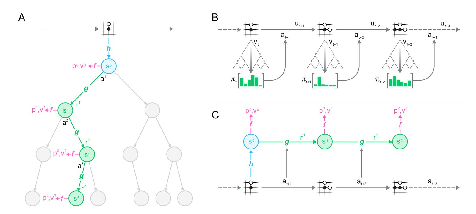
Figure 1: Planning, acting, and training with a learned model. (A) How MuZero uses its model to plan. The model consists of three connected components for representation, dynamics and prediction. Given a previous hidden state and a candidate action , the dynamics function produces an immediate reward and a new hidden state . The policy and value function are computed from the hidden state by a prediction function . The initial hidden state is obtained by passing the past observations (e.g. the Go board or Atari screen) into a representation function . (B) How MuZero acts in the environment. A Monte-Carlo Tree Search is performed at each timestep , as described in A. An action is sampled from the search policy , which is proportional to the visit count for each action from the root node. The environment receives the action and generates a new observation and reward . At the end of the episode the trajectory data is stored into a replay buffer. (C) How MuZero trains its model. A trajectory is sampled from the replay buffer. For the initial step, the representation function receives as input the past observations from the selected trajectory. The model is subsequently unrolled recurrently for steps. At each step , the dynamics function receives as input the hidden state from the previous step and the real action . The parameters of the representation, dynamics and prediction functions are jointly trained, end-to-end by backpropagation-through-time, to predict three quantities: the policy , value function , and reward , where is a sample return: either the final reward (board games) or -step return (Atari).
图 1:用学得的模型做规划、行动与训练。 (A) MuZero 如何用模型规划。模型由表示、动力学与预测三个相连组件构成。给定上一隐状态 与候选动作 ,动力学函数 产生即时奖励 与新隐状态 。策略 与价值函数 由预测函数 从隐状态 算出。初始隐状态 由把过去观测(如围棋盘或 Atari 画面)送入表示函数 得到。(B) MuZero 如何在环境中行动。每个时间步 做一次蒙特卡洛树搜索,如 A 所述。动作 从搜索策略 采样,该策略与根节点各动作的访问次数成正比。环境接收动作并产生新观测 与奖励 。回合结束时轨迹存入回放缓冲。(C) MuZero 如何训练模型。从回放缓冲采样一条轨迹。初始步,表示函数 以所选轨迹的过去观测 为输入。随后模型循环展开 步。每一步 ,动力学函数 以先前步的隐状态 与真实动作 为输入。表示、动力学与预测函数的参数经沿时间反向传播端到端联合训练,以预测三项量:策略 、价值函数 、奖励 ,其中 为样本回报:棋类为终局奖励,Atari 为 步回报。
We now describe the MuZero algorithm in more detail. Predictions are made at each time-step , for each of steps, by a model , with parameters , conditioned on past observations and future actions . The model predicts three future quantities: the policy , the value function , and the immediate reward , where is the true, observed reward, is the policy used to select real actions, and is the discount function of the environment.
下面更细致地描述 MuZero。在每个时间步 ,对 的每一步,由参数为 的模型 ,以过去观测 与未来动作 为条件做预测。模型预测三项未来量:策略 ,价值函数 ,以及即时奖励 ,其中 为真实观测奖励, 为选择真实动作的策略, 为环境折扣。
Internally, at each time-step (subscripts t suppressed for simplicity), the model is represented by the combination of a representation function, a dynamics function, and a prediction function. The dynamics function, , is a recurrent process that computes, at each hypothetical step , an immediate reward and an internal state . It mirrors the structure of an MDP model that computes the expected reward and state transition for a given state and action [31]. However, unlike traditional approaches to model-based RL [42], this internal state has no semantics of environment state attached to it – it is simply the hidden state of the overall model, and its sole purpose is to accurately predict relevant, future quantities: policies, values, and rewards. In this paper, the dynamics function is represented deterministically; the extension to stochastic transitions is left for future work. The policy and value functions are computed from the internal state by the prediction function, , akin to the joint policy and value network of AlphaZero. The “root” state is initialized using a representation function that encodes past observations, ; again this has no special semantics beyond its support for future predictions.
在内部,每个时间步 (为简洁省略下标 t)模型由表示函数、动力学函数与预测函数组合而成。动力学函数 是一个循环过程,在每个假设步 计算即时奖励 与内部状态 。它镜像了给定状态与动作计算期望奖励与状态转移的 MDP 模型结构 [31]。但与传统基于模型 RL [42] 不同,内部状态 并不附着环境状态的语义——它只是整体模型的隐状态,唯一目的是准确预测相关的未来量:策略、价值与奖励。本文中动力学函数用确定性表示;扩展到随机转移留待未来工作。策略与价值由预测函数从内部状态算出:,类似 AlphaZero 的联合策略–价值网络。「根」状态 由编码过去观测的表示函数初始化:;同样,除支持未来预测外并无特殊语义。
Given such a model, it is possible to search over hypothetical future trajectories given past observations . For example, a naive search could simply select the step action sequence that maximizes the value function. More generally, we may apply any MDP planning algorithm to the internal rewards and state space induced by the dynamics function. Specifically, we use an MCTS algorithm similar to AlphaZero’s search, generalized to allow for single agent domains and intermediate rewards (see Methods). At each internal node, it makes use of the policy, value and reward estimates produced by the current model parameters . The MCTS algorithm outputs a recommended policy and estimated value . An action is then selected.
有了这样的模型,便可在给定过去观测 时,对假设未来轨迹 做搜索。例如,朴素搜索可直接选择使价值函数最大的 步动作序列。更一般地,可对动力学函数诱导的内部奖励与状态空间应用任意 MDP 规划算法。具体地,我们使用类似 AlphaZero 搜索、并推广到单智能体领域与中间奖励的 MCTS(见方法)。在每个内部节点,它利用当前模型参数 产生的策略、价值与奖励估计。MCTS 输出推荐策略 与估计价值 ,再采样动作 。
All parameters of the model are trained jointly to accurately match the policy, value, and reward, for every hypothetical step , to corresponding target values observed after actual time-steps have elapsed. Similarly to AlphaZero, the improved policy targets are generated by an MCTS search; the first objective is to minimise the error between predicted policy and search policy . Also like AlphaZero, the improved value targets are generated by playing the game or MDP. However, unlike AlphaZero, we allow for long episodes with discounting and intermediate rewards by bootstrapping steps into the future from the search value, . Final outcomes in board games are treated as rewards occuring at the final step of the episode. Specifically, the second objective is to minimize the error between the predicted value and the value target, [^1]. The reward targets are simply the observed rewards; the third objective is therefore to minimize the error between the predicted reward and the observed reward . Finally, an L2 regularization term is also added, leading to the overall loss:
模型全部参数联合训练,使每个假设步 的策略、价值与奖励,准确匹配 个实际时间步之后观测到的对应目标。与 AlphaZero 类似,改进的策略目标由 MCTS 搜索生成;第一目标是最小化预测策略 与搜索策略 的误差。同样类似 AlphaZero,改进的价值目标通过实际对局或 MDP 交互生成。但与 AlphaZero 不同,我们允许长回合、折扣与中间奖励,通过从搜索价值向未来自举 步:。棋类终局结果 视为回合最后一步出现的奖励 。具体地,第二目标是最小化预测价值 与价值目标 的误差[^1]。奖励目标即观测奖励;第三目标是最小化预测奖励 与观测奖励 的误差。最后再加 L2 正则项,得到总损失:
where , , and are loss functions for reward, value and policy respectively. Supplementary Figure S2 summarizes the equations governing how the MuZero algorithm plans, acts, and learns.
其中 、、 分别为奖励、价值与策略的损失函数。补充图 S2 汇总了 MuZero 规划、行动与学习的方程。
4 Results
4 结果
| Chess | Shogi | Go | Atari |
|---|---|---|---|
| \newgame \newgame\notationoff\showboard | |||
Figure 2: Evaluation of MuZero throughout training in chess, shogi, Go and Atari. The x-axis shows millions of training steps. For chess, shogi and Go, the y-axis shows Elo rating, established by playing games against AlphaZero using 800 simulations per move for both players. MuZero’s Elo is indicated by the blue line, AlphaZero’s Elo by the horizontal orange line. For Atari, mean (full line) and median (dashed line) human normalized scores across all 57 games are shown on the y-axis. The scores for R2D2 [21], (the previous state of the art in this domain, based on model-free RL) are indicated by the horizontal orange lines. Performance in Atari was evaluated using 50 simulations every fourth time-step, and then repeating the chosen action four times, as in prior work [25].
| 国际象棋 | 将棋 | 围棋 | Atari |
|---|---|---|---|
图 2:MuZero 在国际象棋、将棋、围棋与 Atari 训练全程的评估。 横轴为百万训练步。棋类纵轴为 Elo:双方每步 800 次模拟对 AlphaZero 对弈得到。蓝线为 MuZero 的 Elo,橙水平线为 AlphaZero。Atari 纵轴为 57 款游戏上人类归一化分数的均值(实线)与中位数(虚线)。R2D2 [21](该领域先前最优、基于无模型 RL)以橙水平线标出。Atari 评估每四步用 50 次模拟,再把所选动作重复四次,与先前工作一致 [25]。
We applied the MuZero algorithm to the classic board games Go, chess and shogi [^2], as benchmarks for challenging planning problems, and to all 57 games in the Atari Learning Environment [2], as benchmarks for visually complex RL domains.
我们将 MuZero 用于经典棋类围棋、国际象棋与将棋[^2]作为挑战性规划基准,并用于 Atari Learning Environment [2] 全部 57 款游戏作为视觉复杂 RL 基准。
In each case we trained MuZero for hypothetical steps. Training proceeded for 1 million mini-batches of size 2048 in board games and of size 1024 in Atari. During both training and evaluation, MuZero used 800 simulations for each search in board games, and 50 simulations for each search in Atari. The representation function uses the same convolutional [23] and residual [15] architecture as AlphaZero, but with 16 residual blocks instead of 20. The dynamics function uses the same architecture as the representation function and the prediction function uses the same architecture as AlphaZero. All networks use 256 hidden planes (see Methods for further details).
每种情形下 MuZero 以 假设步训练。棋类训练 100 万个大小为 2048 的小批量,Atari 为 1024。训练与评估时,棋类每次搜索 800 次模拟,Atari 为 50 次。表示函数使用与 AlphaZero 相同的卷积 [23] 与残差 [15] 结构,但残差块为 16 而非 20。动力学函数与表示函数同构,预测函数与 AlphaZero 同构。所有网络使用 256 个隐平面(细节见方法)。
Figure 2 shows the performance throughout training in each game. In Go, MuZero slightly exceeded the performance of AlphaZero, despite using less computation per node in the search tree (16 residual blocks per evaluation in MuZero compared to 20 blocks in AlphaZero). This suggests that MuZero may be caching its computation in the search tree and using each additional application of the dynamics model to gain a deeper understanding of the position.
图 2 给出各游戏训练全程表现。在围棋上,MuZero 略超 AlphaZero,尽管搜索树每个节点的计算更少(MuZero 每次评估 16 个残差块,AlphaZero 为 20)。这暗示 MuZero 可能在搜索树中缓存计算,并用每一次额外的动力学模型应用加深对局面的理解。
In Atari, MuZero achieved a new state of the art for both mean and median normalized score across the 57 games of the Arcade Learning Environment, outperforming the previous state-of-the-art method R2D2 [21] (a model-free approach) in 42 out of 57 games, and outperforming the previous best model-based approach SimPLe [20] in all games (see Table S1).
在 Atari 上,MuZero 在 Arcade Learning Environment 57 款游戏的均值与中位数归一化分数上都刷新了当时最优,在 42/57 款游戏上超过先前最优方法 R2D2 [21](无模型),并在全部游戏上超过先前最好的基于模型方法 SimPLe [20](见表 S1)。
We also evaluated a second version of MuZero that was optimised for greater sample efficiency. Specifically, it reanalyzes old trajectories by re-running the MCTS using the latest network parameters to provide fresh targets (see Appendix H). When applied to 57 Atari games, using 200 million frames of experience per game, MuZero Reanalyze achieved 731% median normalized score, compared to 192%, 231% and 431% for previous state-of-the-art model-free approaches IMPALA [9], Rainbow [17] and LASER [36] respectively.
我们还评估了为更高样本效率优化的第二版 MuZero。具体地,它用最新网络参数重跑 MCTS,对旧轨迹做再分析以提供新目标(见附录 H)。在 57 款 Atari、每游戏 2 亿帧经验上,MuZero Reanalyze 达到 731% 中位数归一化分数,而先前最优无模型方法 IMPALA [9]、Rainbow [17]、LASER [36] 分别为 192%、231%、431%。
| Agent | Median | Mean | Env. Frames | Training Time | Training Steps |
|---|---|---|---|---|---|
| Ape-X [18] | 434.1% | 1695.6% | 22.8B | 5 days | 8.64M |
| R2D2 [21] | 1920.6% | 4024.9% | 37.5B | 5 days | 2.16M |
| MuZero | 2041.1% | 4999.2% | 20.0B | 12 hours | 1M |
| IMPALA [9] | 191.8% | 957.6% | 200M | – | – |
| Rainbow [17] | 231.1% | – | 200M | 10 days | – |
| UNREALa [19] | 250%a | 880%a | 250M | – | – |
| LASER [36] | 431% | – | 200M | – | – |
| MuZero Reanalyze | 731.1% | 2168.9% | 200M | 12 hours | 1M |
Table 1: Comparison of MuZero against previous agents in Atari. We compare separately against agents trained in large (top) and small (bottom) data settings; all agents other than MuZero used model-free RL techniques. Mean and median scores are given, compared to human testers. The best results are highlighted in bold. MuZero sets a new state of the art in both settings. aHyper-parameters were tuned per game.
| Agent | Median | Mean | Env. Frames | Training Time | Training Steps |
|---|---|---|---|---|---|
| Ape-X [18] | 434.1% | 1695.6% | 22.8B | 5 days | 8.64M |
| R2D2 [21] | 1920.6% | 4024.9% | 37.5B | 5 days | 2.16M |
| MuZero | 2041.1% | 4999.2% | 20.0B | 12 hours | 1M |
| IMPALA [9] | 191.8% | 957.6% | 200M | – | – |
| Rainbow [17] | 231.1% | – | 200M | 10 days | – |
| UNREALa [19] | 250%a | 880%a | 250M | – | – |
| LASER [36] | 431% | – | 200M | – | – |
| MuZero Reanalyze | 731.1% | 2168.9% | 200M | 12 hours | 1M |
表 1:MuZero 与先前 Atari 智能体的比较。 分别对比大数据(上)与小数据(下)设定;除 MuZero 外均为无模型 RL。给出相对人类测试者的均值与中位数分数。最优结果加粗。MuZero 在两种设定都刷新了当时最优。a 超参按游戏调。
To understand the role of the model in MuZero we also ran several experiments, focusing on the board game of Go and the Atari game of Ms. Pacman.
为理解模型在 MuZero 中的作用,我们还做了若干实验,聚焦围棋与 Atari 的 Ms. Pacman。
First, we tested the scalability of planning (Figure 3A), in the canonical planning problem of Go. We compared the performance of search in AlphaZero, using a perfect model, to the performance of search in MuZero, using a learned model. Specifically, the fully trained AlphaZero or MuZero was evaluated by comparing MCTS with different thinking times. MuZero matched the performance of a perfect model, even when doing much larger searches (up to 10s thinking time) than those from which the model was trained (around 0.1s thinking time, see also Figure S3A).
首先,在经典规划问题围棋上测试规划的可扩展性(图 3A)。我们比较 AlphaZero 用完美模型做搜索的表现,与 MuZero 用学得模型做搜索的表现。具体地,对充分训练的 AlphaZero 或 MuZero,用不同思考时间的 MCTS 评估。即便做远大于训练时(约 0.1 秒思考时间,亦见图 S3A)的搜索(最长约 10 秒),MuZero 仍匹配完美模型的表现。
We also investigated the scalability of planning across all Atari games (see Figure 3B). We compared MCTS with different numbers of simulations, using the fully trained MuZero. The improvements due to planning are much less marked than in Go, perhaps because of greater model inaccuracy; performance improved slightly with search time, but plateaued at around 100 simulations. Even with a single simulation – i.e. when selecting moves solely according to the policy network – MuZero performed well, suggesting that, by the end of training, the raw policy has learned to internalise the benefits of search (see also Figure S3B).
我们还考察了全部 Atari 游戏上规划的可扩展性(图 3B)。对充分训练的 MuZero,比较不同模拟次数的 MCTS。相对围棋,由规划带来的提升不那么明显,可能因模型误差更大;表现随搜索时间略有提升,约在 100 次模拟处平台。即便仅一次模拟——即完全按策略网络选招——MuZero 仍表现良好,说明训练末期原始策略已把搜索的收益内化(亦见图 S3B)。
Next, we tested our model-based learning algorithm against a comparable model-free learning algorithm (see Figure 3C). We replaced the training objective of MuZero (Equation 1) with a model-free Q-learning objective (as used by R2D2), and the dual value and policy heads with a single head representing the Q-function . Subsequently, we trained and evaluated the new model without using any search. When evaluated on Ms. Pacman, our model-free algorithm achieved identical results to R2D2, but learned significantly slower than MuZero and converged to a much lower final score. We conjecture that the search-based policy improvement step of MuZero provides a stronger learning signal than the high bias, high variance targets used by Q-learning.
接着,我们把基于模型的学习算法与可比的无模型学习算法对比(图 3C)。用无模型 Q-learning 目标(如 R2D2)替换 MuZero 的训练目标(式 1),并把双头价值与策略换成表示 Q 函数 的单头。随后在不使用任何搜索的情况下训练与评估新模型。在 Ms. Pacman 上,我们的无模型算法达到与 R2D2 相同的结果,但学习显著慢于 MuZero,最终分数也低得多。我们推测 MuZero 基于搜索的策略改进步骤,提供了比 Q-learning 所用高偏、高方差目标更强的学习信号。
To better understand the nature of MuZero’s learning algorithm, we measured how MuZero’s training scales with respect to the amount of search it uses during training. Figure 3D shows the performance in Ms. Pacman, using an MCTS of different simulation counts per move throughout training. Surprisingly, and in contrast to previous work [1], even with only 6 simulations per move – fewer than the number of actions – MuZero learned an effective policy and improved rapidly. With more simulations performance jumped significantly higher. For analysis of the policy improvement during each individual iteration, see also Figure S3 C and D.
为更好理解 MuZero 学习算法的性质,我们测量训练过程中所用搜索量如何影响训练缩放。图 3D 给出 Ms. Pacman 上、训练全程每步不同模拟次数的 MCTS 表现。令人惊讶的是,与先前工作 [1] 相反,即便每步仅 6 次模拟——少于动作数——MuZero 仍学到有效策略并快速改进。更多模拟时表现显著跃升。各迭代内策略改进分析亦见图 S3 C 与 D。

Figure 3: Evaluations of MuZero on Go (A), all 57 Atari Games (B) and Ms. Pacman (C-D). (A) Scaling with search time per move in Go, comparing the learned model with the ground truth simulator. Both networks were trained at 800 simulations per search, equivalent to 0.1 seconds per search. Remarkably, the learned model is able to scale well to up to two orders of magnitude longer searches than seen during training. (B) Scaling of final human normalized mean score in Atari with the number of simulations per search. The network was trained at 50 simulations per search. Dark line indicates mean score, shaded regions indicate 25th to 75th and 5th to 95th percentiles. The learned model’s performance increases up to 100 simulations per search. Beyond, even when scaling to much longer searches than during training, the learned model’s performance remains stable and only decreases slightly. This contrasts with the much better scaling in Go (A), presumably due to greater model inaccuracy in Atari than Go. (C) Comparison of MCTS based training with Q-learning in the MuZero framework on Ms. Pacman, keeping network size and amount of training constant. The state of the art Q-Learning algorithm R2D2 is shown as a baseline. Our Q-Learning implementation reaches the same final score as R2D2, but improves slower and results in much lower final performance compared to MCTS based training. (D) Different networks trained at different numbers of simulations per move, but all evaluated at 50 simulations per move. Networks trained with more simulations per move improve faster, consistent with ablation (B), where the policy improvement is larger when using more simulations per move. Surprisingly, MuZero can learn effectively even when training with less simulations per move than are enough to cover all 8 possible actions in Ms. Pacman.
图 3:MuZero 在围棋 (A)、全部 57 款 Atari (B) 与 Ms. Pacman (C-D) 上的评估。 (A) 围棋中每步搜索时间的缩放,比较学得模型与真实模拟器。两网络均以每次搜索 800 次模拟训练,约合每次搜索 0.1 秒。学得模型可良好扩展到比训练时长两数量级的搜索。(B) Atari 最终人类归一化均值分数随每次搜索模拟次数的缩放。网络以 50 次模拟训练。深线为均值,阴影为第 25–75 与第 5–95 百分位。学得模型表现提升至约 100 次模拟;再更长时仍稳定、仅略降。与围棋 (A) 中更好的缩放形成对比,推测因 Atari 模型误差更大。(C) 在 MuZero 框架内、固定网络规模与训练量,比较基于 MCTS 的训练与 Q-learning(Ms. Pacman)。当时最优 Q-Learning 算法 R2D2 作基线。我们的 Q-Learning 实现达到与 R2D2 相同的最终分数,但改进更慢,最终表现远低于基于 MCTS 的训练。(D) 以不同每步模拟次数训练的网络,均在 50 次模拟下评估。训练时模拟更多则改进更快,与消融 (B) 一致:更多模拟时策略改进更大。令人惊讶的是,即便训练时每步模拟少于覆盖 Ms. Pacman 全部 8 个可能动作所需,MuZero 仍能有效学习。
5 Conclusions
5 结论
Many of the breakthroughs in artificial intelligence have been based on either high-performance planning [5, 38, 39] or model-free reinforcement learning methods [25, 29, 46]. In this paper we have introduced a method that combines the benefits of both approaches. Our algorithm, MuZero, has both matched the superhuman performance of high-performance planning algorithms in their favored domains – logically complex board games such as chess and Go – and outperformed state-of-the-art model-free RL algorithms in their favored domains – visually complex Atari games. Crucially, our method does not require any knowledge of the game rules or environment dynamics, potentially paving the way towards the application of powerful learning and planning methods to a host of real-world domains for which there exists no perfect simulator.
人工智能的许多突破建立在高性能规划 [5, 38, 39] 或无模型强化学习 [25, 29, 46] 之上。本文提出一种兼具两者优势的方法。我们的算法 MuZero,既在其擅长的领域——逻辑复杂的棋类如国际象棋与围棋——匹配高性能规划算法的超人类水平,又在其擅长的领域——视觉复杂的 Atari——超过当时最优的无模型 RL。关键是,本方法不需要任何游戏规则或环境动力学知识,有望把强大的学习与规划方法推向大量不存在完美模拟器的现实领域。
6 Acknowledgments
6 致谢
Lorrayne Bennett, Oliver Smith and Chris Apps for organizational assistance; Koray Kavukcuoglu for reviewing the paper; Thomas Anthony, Matthew Lai, Nenad Tomasev, Ulrich Paquet, Sumedh Ghaisas for many fruitful discussions; and the rest of the DeepMind team for their support.
感谢 Lorrayne Bennett、Oliver Smith 与 Chris Apps 的组织协助;Koray Kavukcuoglu 审阅论文;Thomas Anthony、Matthew Lai、Nenad Tomasev、Ulrich Paquet、Sumedh Ghaisas 的诸多有益讨论;以及 DeepMind 团队其余成员的支持。
References
参考文献
[1] Kamyar Azizzadenesheli, Brandon Yang, Weitang Liu, Emma Brunskill, Zachary C. Lipton, and Animashree Anandkumar. Surprising negative results for generative adversarial tree search. CoRR , abs/1806.05780, 2018.
[2] Marc G Bellemare, Yavar Naddaf, Joel Veness, and Michael Bowling. The arcade learning environment: An evaluation platform for general agents. Journal of Artificial Intelligence Research , 47:253–279, 2013.
[3] Noam Brown and Tuomas Sandholm. Superhuman ai for heads-up no-limit poker: Libratus beats top professionals. Science , 359(6374):418–424, 2018.
[4] Lars Buesing, Theophane Weber, Sebastien Racaniere, SM Eslami, Danilo Rezende, David P Reichert, Fabio Viola, Frederic Besse, Karol Gregor, Demis Hassabis, et al. Learning and querying fast generative models for reinforcement learning. arXiv preprint arXiv:1802.03006 , 2018.
[5] Murray Campbell, A. Joseph Hoane, Jr., and Feng-hsiung Hsu. Deep blue. Artif. Intell. , 134(1-2):57–83, January 2002.
[6] R. Coulom. Whole-history rating: A Bayesian rating system for players of time-varying strength. In International Conference on Computers and Games , pages 113–124, 2008.
[7] Rémi Coulom. Efficient selectivity and backup operators in monte-carlo tree search. In International conference on computers and games , pages 72–83. Springer, 2006.
[8] MP. Deisenroth and CE. Rasmussen. Pilco: A model-based and data-efficient approach to policy search. In Proceedings of the 28th International Conference on Machine Learning, ICML 2011 , pages 465–472. Omnipress, 2011.
[9] Lasse Espeholt, Hubert Soyer, Remi Munos, Karen Simonyan, Volodymir Mnih, Tom Ward, Yotam Doron, Vlad Firoiu, Tim Harley, Iain Dunning, et al. Impala: Scalable distributed deep-rl with importance weighted actor-learner architectures. In Proceedings of the International Conference on Machine Learning (ICML) , 2018.
[10] Gregory Farquhar, Tim Rocktaeschel, Maximilian Igl, and Shimon Whiteson. TreeQN and ATreec: Differentiable tree planning for deep reinforcement learning. In International Conference on Learning Representations , 2018.
[11] Carles Gelada, Saurabh Kumar, Jacob Buckman, Ofir Nachum, and Marc G. Bellemare. DeepMDP: Learning continuous latent space models for representation learning. In Kamalika Chaudhuri and Ruslan Salakhutdinov, editors, Proceedings of the 36th International Conference on Machine Learning , volume 97 of Proceedings of Machine Learning Research , pages 2170–2179, Long Beach, California, USA, 09–15 Jun 2019. PMLR.
[12] Cloud tpu. https://cloud.google.com/tpu/ . Accessed: 2019.
[13] David Ha and Jürgen Schmidhuber. Recurrent world models facilitate policy evolution. In Proceedings of the 32Nd International Conference on Neural Information Processing Systems , NIPS’18, pages 2455–2467, USA, 2018. Curran Associates Inc.
[14] Danijar Hafner, Timothy Lillicrap, Ian Fischer, Ruben Villegas, David Ha, Honglak Lee, and James Davidson. Learning latent dynamics for planning from pixels. arXiv preprint arXiv:1811.04551 , 2018.
[15] Kaiming He, Xiangyu Zhang, Shaoqing Ren, and Jian Sun. Identity mappings in deep residual networks. In 14th European Conference on Computer Vision , pages 630–645, 2016.
[16] Nicolas Heess, Greg Wayne, David Silver, Timothy Lillicrap, Yuval Tassa, and Tom Erez. Learning continuous control policies by stochastic value gradients. In Proceedings of the 28th International Conference on Neural Information Processing Systems - Volume 2 , NIPS’15, pages 2944–2952, Cambridge, MA, USA, 2015. MIT Press.
[17] Matteo Hessel, Joseph Modayil, Hado Van Hasselt, Tom Schaul, Georg Ostrovski, Will Dabney, Dan Horgan, Bilal Piot, Mohammad Azar, and David Silver. Rainbow: Combining improvements in deep reinforcement learning. In Thirty-Second AAAI Conference on Artificial Intelligence , 2018.
[18] Dan Horgan, John Quan, David Budden, Gabriel Barth-Maron, Matteo Hessel, Hado van Hasselt, and David Silver. Distributed prioritized experience replay. In International Conference on Learning Representations , 2018.
[19] Max Jaderberg, Volodymyr Mnih, Wojciech Marian Czarnecki, Tom Schaul, Joel Z Leibo, David Silver, and Koray Kavukcuoglu. Reinforcement learning with unsupervised auxiliary tasks. arXiv preprint arXiv:1611.05397 , 2016.
[20] Lukasz Kaiser, Mohammad Babaeizadeh, Piotr Milos, Blazej Osinski, Roy H Campbell, Konrad Czechowski, Dumitru Erhan, Chelsea Finn, Piotr Kozakowski, Sergey Levine, et al. Model-based reinforcement learning for atari. arXiv preprint arXiv:1903.00374 , 2019.
[21] Steven Kapturowski, Georg Ostrovski, Will Dabney, John Quan, and Remi Munos. Recurrent experience replay in distributed reinforcement learning. In International Conference on Learning Representations , 2019.
[22] Levente Kocsis and Csaba Szepesvári. Bandit based monte-carlo planning. In European conference on machine learning , pages 282–293. Springer, 2006.
[23] Alex Krizhevsky, Ilya Sutskever, and Geoffrey E Hinton. Imagenet classification with deep convolutional neural networks. In Advances in neural information processing systems , pages 1097–1105, 2012.
[24] Sergey Levine and Pieter Abbeel. Learning neural network policies with guided policy search under unknown dynamics. In Z. Ghahramani, M. Welling, C. Cortes, N. D. Lawrence, and K. Q. Weinberger, editors, Advances in Neural Information Processing Systems 27 , pages 1071–1079. Curran Associates, Inc., 2014.
[25] Volodymyr Mnih, Koray Kavukcuoglu, David Silver, Andrei A Rusu, Joel Veness, Marc G Bellemare, Alex Graves, Martin Riedmiller, Andreas K Fidjeland, Georg Ostrovski, et al. Human-level control through deep reinforcement learning. Nature , 518(7540):529, 2015.
[26] Matej Moravčík, Martin Schmid, Neil Burch, Viliam Lisỳ, Dustin Morrill, Nolan Bard, Trevor Davis, Kevin Waugh, Michael Johanson, and Michael Bowling. Deepstack: Expert-level artificial intelligence in heads-up no-limit poker. Science , 356(6337):508–513, 2017.
[27] Arun Nair, Praveen Srinivasan, Sam Blackwell, Cagdas Alcicek, Rory Fearon, Alessandro De Maria, Vedavyas Panneershelvam, Mustafa Suleyman, Charles Beattie, Stig Petersen, Shane Legg, Volodymyr Mnih, Koray Kavukcuoglu, and David Silver. Massively parallel methods for deep reinforcement learning. CoRR , abs/1507.04296, 2015.
[28] Junhyuk Oh, Satinder Singh, and Honglak Lee. Value prediction network. In Advances in Neural Information Processing Systems , pages 6118–6128, 2017.
[29] OpenAI. Openai five. https://blog.openai.com/openai-five/ , 2018.
[30] Tobias Pohlen, Bilal Piot, Todd Hester, Mohammad Gheshlaghi Azar, Dan Horgan, David Budden, Gabriel Barth-Maron, Hado van Hasselt, John Quan, Mel Večerík, et al. Observe and look further: Achieving consistent performance on atari. arXiv preprint arXiv:1805.11593 , 2018.
[31] Martin L. Puterman. Markov Decision Processes: Discrete Stochastic Dynamic Programming . John Wiley & Sons, Inc., New York, NY, USA, 1st edition, 1994.
[32] Christopher D Rosin. Multi-armed bandits with episode context. Annals of Mathematics and Artificial Intelligence , 61(3):203–230, 2011.
[33] Maarten PD Schadd, Mark HM Winands, H Jaap Van Den Herik, Guillaume MJ-B Chaslot, and Jos WHM Uiterwijk. Single-player monte-carlo tree search. In International Conference on Computers and Games , pages 1–12. Springer, 2008.
[34] Jonathan Schaeffer, Joseph Culberson, Norman Treloar, Brent Knight, Paul Lu, and Duane Szafron. A world championship caliber checkers program. Artificial Intelligence , 53(2-3):273–289, 1992.
[35] Tom Schaul, John Quan, Ioannis Antonoglou, and David Silver. Prioritized experience replay. In International Conference on Learning Representations , Puerto Rico, 2016.
[36] Simon Schmitt, Matteo Hessel, and Karen Simonyan. Off-policy actor-critic with shared experience replay. arXiv preprint arXiv:1909.11583 , 2019.
[37] Marwin HS Segler, Mike Preuss, and Mark P Waller. Planning chemical syntheses with deep neural networks and symbolic ai. Nature , 555(7698):604, 2018.
[38] David Silver, Aja Huang, Chris J. Maddison, Arthur Guez, Laurent Sifre, George van den Driessche, Julian Schrittwieser, Ioannis Antonoglou, Veda Panneershelvam, Marc Lanctot, Sander Dieleman, Dominik Grewe, John Nham, Nal Kalchbrenner, Ilya Sutskever, Timothy Lillicrap, Madeleine Leach, Koray Kavukcuoglu, Thore Graepel, and Demis Hassabis. Mastering the game of Go with deep neural networks and tree search. Nature , 529(7587):484–489, January 2016.
[39] David Silver, Thomas Hubert, Julian Schrittwieser, Ioannis Antonoglou, Matthew Lai, Arthur Guez, Marc Lanctot, Laurent Sifre, Dharshan Kumaran, Thore Graepel, et al. A general reinforcement learning algorithm that masters chess, shogi, and go through self-play. Science , 362(6419):1140–1144, 2018.
[40] David Silver, Julian Schrittwieser, Karen Simonyan, Ioannis Antonoglou, Aja Huang, Arthur Guez, Thomas Hubert, Lucas Baker, Matthew Lai, Adrian Bolton, Yutian Chen, Timothy Lillicrap, Fan Hui, Laurent Sifre, George van den Driessche, Thore Graepel, and Demis Hassabis. Mastering the game of go without human knowledge. Nature , 550:354–359, October 2017.
[41] David Silver, Hado van Hasselt, Matteo Hessel, Tom Schaul, Arthur Guez, Tim Harley, Gabriel Dulac-Arnold, David Reichert, Neil Rabinowitz, Andre Barreto, et al. The predictron: End-to-end learning and planning. In Proceedings of the 34th International Conference on Machine Learning-Volume 70 , pages 3191–3199. JMLR. org, 2017.
[42] Richard S. Sutton and Andrew G. Barto. Reinforcement Learning: An Introduction . The MIT Press, second edition, 2018.
[43] Richard S Sutton, Doina Precup, and Satinder Singh. Between mdps and semi-mdps: A framework for temporal abstraction in reinforcement learning. Artificial intelligence , 112(1-2):181–211, 1999.
[44] Aviv Tamar, Yi Wu, Garrett Thomas, Sergey Levine, and Pieter Abbeel. Value iteration networks. In Advances in Neural Information Processing Systems , pages 2154–2162, 2016.
[45] Hado van Hasselt, Matteo Hessel, and John Aslanides. When to use parametric models in reinforcement learning? arXiv preprint arXiv:1906.05243 , 2019.
[46] Oriol Vinyals, Igor Babuschkin, Wojciech M Czarnecki, Michaël Mathieu, Andrew Dudzik, Junyoung Chung, David H Choi, Richard Powell, Timo Ewalds, Petko Georgiev, et al. Grandmaster level in StarCraft II using multi-agent reinforcement learning. Nature , pages 1–5, 2019.
[47] I Vlahavas and I Refanidis. Planning and scheduling. EETN, Greece, Tech. Rep , 2013.
[48] Niklas Wahlström, Thomas B. Schön, and Marc Peter Deisenroth. From pixels to torques: Policy learning with deep dynamical models. CoRR , abs/1502.02251, 2015.
[49] Manuel Watter, Jost Tobias Springenberg, Joschka Boedecker, and Martin Riedmiller. Embed to control: A locally linear latent dynamics model for control from raw images. In Proceedings of the 28th International Conference on Neural Information Processing Systems - Volume 2 , NIPS’15, pages 2746–2754, Cambridge, MA, USA, 2015. MIT Press.
Supplementary Materials
补充材料
- • Pseudocode description of the MuZero algorithm.
- • Data for Figures 2, 3, S2, S3, S4 and Tables 1, S1, S2 in JSON format.
- • MuZero 算法的伪代码描述。
- • 图 2、3、S2、S3、S4 与表 1、S1、S2 的 JSON 数据。
Supplementary materials can be accessed from the ancillary file section of the arXiv submission.
补充材料可从 arXiv 投稿的附属文件区获取。
Appendix A Comparison to AlphaZero
附录 A 与 AlphaZero 的比较
MuZero is designed for a more general setting than AlphaGo Zero [40] and AlphaZero [39].
MuZero 面向比 AlphaGo Zero [40] 与 AlphaZero [39] 更一般的设定。
In AlphaGo Zero and AlphaZero the planning process makes use of two separate components: a simulator implements the rules of the game, which are used to update the state of the game while traversing the search tree; and a neural network jointly predicts the corresponding policy and value of a board position produced by the simulator (see Figure 1 A).
在 AlphaGo Zero 与 AlphaZero 中,规划过程使用两个独立组件:模拟器实现游戏规则,用于在遍历搜索树时更新局面;神经网络联合预测模拟器产生的盘面所对应的策略与价值(见图 1 A)。
Specifically, AlphaGo Zero and AlphaZero use knowledge of the rules of the game in three places: (1) state transitions in the search tree, (2) actions available at each node of the search tree, (3) episode termination within the search tree. In MuZero, all of these have been replaced with the use of a single implicit model learned by a neural network (see Figure 1 B):
具体地,AlphaGo Zero 与 AlphaZero 在三处使用规则知识:(1) 搜索树中的状态转移,(2) 搜索树各节点可用的动作,(3) 搜索树内的回合终止。在 MuZero 中,这些都由神经网络学到的单一隐式模型取代(见图 1 B):
- State transitions. AlphaZero had access to a perfect simulator of the true dynamics process. In contrast, MuZero employs a learned dynamics model within its search. Under this model, each node in the tree is represented by a corresponding hidden state; by providing a hidden state and an action to the model the search algorithm can transition to a new node = .
- Actions available. AlphaZero used the set of legal actions obtained from the simulator to mask the prior produced by the network everywhere in the search tree. MuZero only masks legal actions at the root of the search tree where the environment can be queried, but does not perform any masking within the search tree. This is possible because the network rapidly learns not to predict actions that never occur in the trajectories it is trained on.
- Terminal nodes. AlphaZero stopped the search at tree nodes representing terminal states and used the terminal value provided by the simulator instead of the value produced by the network. MuZero does not give special treatment to terminal nodes and always uses the value predicted by the network. Inside the tree, the search can proceed past a terminal node - in this case the network is expected to always predict the same value. This is achieved by treating terminal states as absorbing states during training.
- 状态转移。AlphaZero 可访问真实动力学过程的完美模拟器。相比之下,MuZero 在搜索中使用学得的动力学模型。在该模型下,树中每个节点由对应隐状态表示;向模型提供隐状态 与动作 ,搜索算法可转移到新节点 = 。
- 可用动作。AlphaZero 用模拟器得到的合法动作集合,在搜索树各处掩码网络产生的先验。MuZero 仅在可查询环境的搜索树根处掩码合法动作,树内不做掩码。这之所以可行,是因为网络会迅速学会不预测训练轨迹中从未出现的动作。
- 终止节点。AlphaZero 在表示终止状态的树节点停止搜索,并用模拟器提供的终止价值替代网络价值。MuZero 不对终止节点做特殊处理,始终使用网络预测的价值。树内搜索可越过终止节点——此时期望网络始终预测相同价值。训练时把终止状态当作吸收态即可实现。
In addition, MuZero is designed to operate in the general reinforcement learning setting: single-agent domains with discounted intermediate rewards of arbitrary magnitude. In contrast, AlphaGo Zero and AlphaZero were designed to operate in two-player games with undiscounted terminal rewards of .
此外,MuZero 面向一般强化学习设定:带任意幅度折扣中间奖励的单智能体领域。相比之下,AlphaGo Zero 与 AlphaZero 面向终局奖励为 、无折扣的双人博弈。
Appendix B Search
附录 B 搜索
We now describe the search algorithm used by MuZero. Our approach is based upon Monte-Carlo tree search with upper confidence bounds, an approach to planning that converges asymptotically to the optimal policy in single agent domains and to the minimax value function in zero sum games [22].
下面描述 MuZero 使用的搜索算法。方法基于带上置信界的蒙特卡洛树搜索,该规划方法在单智能体领域渐近收敛到最优策略,在零和博弈中收敛到极小极大价值函数 [22]。
Every node of the search tree is associated with an internal state . For each action from there is an edge that stores a set of statistics , respectively representing visit counts , mean value , policy , reward , and state transition .
搜索树每个节点关联一个内部状态 。对从 出发的每个动作 ,边 存储统计量集合 ,分别表示访问次数 、均值价值 、策略 、奖励 与状态转移 。
Similar to AlphaZero, the search is divided into three stages, repeated for a number of simulations.
与 AlphaZero 类似,搜索分为三个阶段,按模拟次数重复。
Selection: Each simulation starts from the internal root state , and finishes when the simulation reaches a leaf node . For each hypothetical time-step of the simulation, an action is selected according to the stored statistics for internal state , by maximizing over an upper confidence bound [32][39],
选择:每次模拟从内部根状态 出发,到达叶节点 结束。对模拟的每个假设时间步 ,根据内部状态 存储的统计量,通过最大化上置信界选择动作 [32][39],
The constants and are used to control the influence of the prior relative to the value as nodes are visited more often. In our experiments, and .
常数 与 用于在节点被访问更频繁时,控制先验 相对价值 的影响。实验中 ,。
For , the next state and reward are looked up in the state transition and reward table , .
对 ,下一状态与奖励在状态转移与奖励表中查找:,。
Expansion: At the final time-step of the simulation, the reward and state are computed by the dynamics function, , and stored in the corresponding tables, . The policy and value are computed by the prediction function, . A new node, corresponding to state is added to the search tree. Each edge from the newly expanded node is initialized to . Note that the search algorithm makes at most one call to the dynamics function and prediction function respectively per simulation; the computational cost is of the same order as in AlphaZero.
扩展:在模拟的最后时间步 ,由动力学函数计算奖励与状态 ,并存入对应表 ,。策略与价值由预测函数计算:。向搜索树加入对应状态 的新节点。从新扩展节点出发的每条边 初始化为 。注意每次模拟至多各调用一次动力学与预测函数;计算代价与 AlphaZero 同阶。
Backup: At the end of the simulation, the statistics along the trajectory are updated. The backup is generalized to the case where the environment can emit intermediate rewards, have a discount different from , and the value estimates are unbounded [^3]. For , we form an -step estimate of the cumulative discounted reward, bootstrapping from the value function ,
回传:模拟结束时更新轨迹上的统计量。回传推广到环境可发出中间奖励、折扣 不必为 1、价值估计无界的情形[^3]。对 ,形成 步累积折扣奖励估计,并从价值函数 自举,
For , we update the statistics for each edge in the simulation path as follows,
对 ,按如下方式更新模拟路径上每条边 的统计量,
In two-player zero sum games the value functions are assumed to be bounded within the interval. This choice allows us to combine value estimates with probabilities using the pUCT rule (Eqn 2). However, since in many environments the value is unbounded, it is necessary to adjust the pUCT rule. A simple solution would be to use the maximum score that can be observed in the environment to either re-scale the value or set the pUCT constants appropriately [33]. However, both solutions are game specific and require adding prior knowledge to the MuZero algorithm. To avoid this, MuZero computes normalized value estimates by using the minimum-maximum values observed in the search tree up to that point. When a node is reached during the selection stage, the algorithm computes the normalized values of its edges to be used in the pUCT rule using the equation below:
在双人零和博弈中,价值函数假定有界于 。这使我们能用 pUCT 规则(式 2)把价值估计与概率结合。但许多环境中价值无界,因而必须调整 pUCT。简单办法是用环境可观测的最大分数重缩放价值,或相应设置 pUCT 常数 [33]。但两者都依赖具体游戏,需向 MuZero 加入先验知识。为避免这一点,MuZero 用截至当时搜索树中观测到的最小–最大价值,计算归一化 估计 。选择阶段到达某节点时,算法用下式计算其边的归一化 以用于 pUCT:
Appendix C Hyperparameters
附录 C 超参数
For simplicity we preferentially use the same architectural choices and hyperparameters as in previous work. Specifically, we started with the network architecture and search choices of AlphaZero [39]. For board games, we use the same UCB constants, dirichlet exploration noise and the same 800 simulations per search as in AlphaZero.
为简洁起见,我们优先沿用先前工作的架构选择与超参数。具体地,从 AlphaZero [39] 的网络架构与搜索选择出发。棋类使用与 AlphaZero 相同的 UCB 常数、Dirichlet 探索噪声,以及每次搜索 800 次模拟。
Due to the much smaller branching factor and simpler policies in Atari, we only used 50 simulations per search to speed up experiments. As shown in Figure 3B, the algorithm is not very sensitive to this choice. We also use the same discount () and value transformation (see Network Architecture section) as R2D2 [21].
因 Atari 分支因子更小、策略更简单,我们只用每次搜索 50 次模拟以加速实验。如图 3B 所示,算法对该选择并不敏感。折扣(0.997)与价值变换(见网络架构一节)也与 R2D2 [21] 相同。
For parameter values not mentioned in the text, please refer to the pseudocode.
文中未提及的参数值请参阅伪代码。
Appendix D Data Generation
附录 D 数据生成
To generate training data, the latest checkpoint of the network (updated every 1000 training steps) is used to play games with MCTS. In the board games Go, chess and shogi the search is run for 800 simulations per move to pick an action; in Atari due to the much smaller action space 50 simulations per move are sufficient.
为生成训练数据,用网络最新检查点(每 1000 训练步更新)以 MCTS 对弈。围棋、国际象棋与将棋每步搜索 800 次模拟选动作;Atari 因动作空间小得多,每步 50 次模拟已足够。
For board games, games are sent to the training job as soon as they finish. Due to the much larger length of Atari games (up to 30 minutes or 108,000 frames), intermediate sequences are sent every 200 moves. In board games, the training job keeps an in-memory replay buffer of the most recent 1 million games received; in Atari, where the visual observations are larger, the most recent 125 thousand sequences of length 200 are kept.
棋类在对局结束后立即把游戏送入训练任务。因 Atari 对局长得多(最长约 30 分钟或 108,000 帧),每 200 步发送中间序列。棋类训练任务在内存中保留最近收到的 100 万局回放缓冲;Atari 视觉观测更大,保留最近 12.5 万条长度为 200 的序列。
During the generation of experience in the board game domains, the same exploration scheme as the one described in AlphaZero [39] is used. Using a variation of this scheme, in the Atari domain actions are sampled from the visit count distribution throughout the duration of each game, instead of just the first moves. Moreover, the visit count distribution is parametrized using a temperature parameter :
棋类经验生成使用与 AlphaZero [39] 相同的探索方案。在此变体下,Atari 在整局过程中都从访问次数分布采样动作,而非仅前 步。此外,访问次数分布用温度参数 参数化:
is decayed as a function of the number of training steps of the network. Specifically, for the first 500k training steps a temperature of is used, for the next 250k steps a temperature of and for the remaining 250k a temperature of . This ensures that the action selection becomes greedier as training progresses.
随网络训练步数衰减。具体地,前 50 万训练步用温度 1,随后 25 万步用 0.5,最后 25 万步用 0.25。这确保随训练推进动作选择更贪婪。
Appendix E Network Input
附录 E 网络输入
Representation Function
表示函数
The history over board states used as input to the representation function for Go, chess and shogi is represented similarly to AlphaZero [39]. In Go and shogi we encode the last 8 board states as in AlphaZero; in chess we increased the history to the last 100 board states to allow correct prediction of draws.
围棋、国际象棋与将棋表示函数输入的盘面历史,表示方式与 AlphaZero [39] 类似。围棋与将棋编码最近 8 个盘面;国际象棋把历史增至最近 100 个盘面,以便正确预测和棋。
For Atari, the input of the representation function includes the last 32 RGB frames at resolution 96x96 along with the last 32 actions that led to each of those frames. We encode the historical actions because unlike board games, an action in Atari does not necessarily have a visible effect on the observation. RGB frames are encoded as one plane per color, rescaled to the range , for red, green and blue respectively. We perform no other normalization, whitening or other preprocessing of the RGB input. Historical actions are encoded as simple bias planes, scaled as (there are 18 total actions in Atari).
对 Atari,表示函数输入包含最近 32 帧 96×96 RGB,以及通向这些帧的最近 32 个动作。我们编码历史动作,因为与棋类不同,Atari 中动作不一定在观测上有可见效果。RGB 帧按红、绿、蓝各一平面编码,缩放到 。不对 RGB 输入做其他归一化、白化或预处理。历史动作编码为简单偏置平面,按 缩放(Atari 共 18 个动作)。
Dynamics Function
动力学函数
The input to the dynamics function is the hidden state produced by the representation function or previous application of the dynamics function, concatenated with a representation of the action for the transition. Actions are encoded spatially in planes of the same resolution as the hidden state. In Atari, this resolution is 6x6 (see description of downsampling in Network Architecture section), in board games this is the same as the board size (19x19 for Go, 8x8 for chess, 9x9 for shogi).
动力学函数的输入是表示函数或上一次动力学应用产生的隐状态,与转移动作的表示拼接。动作在与隐状态同分辨率的平面上空间编码。Atari 该分辨率为 6×6(见网络架构一节的下采样描述);棋类与棋盘大小相同(围棋 19×19,国际象棋 8×8,将棋 9×9)。
In Go, a normal action (playing a stone on the board) is encoded as an all zero plane, with a single one in the position of the played stone. A pass is encoded as an all zero plane.
在围棋中,普通动作(在盘上下子)编码为全零平面,仅在落子位置为 1。停着编码为全零平面。
In chess, 8 planes are used to encode the action. The first one-hot plane encodes which position the piece was moved from. The next two planes encode which position the piece was moved to: a one-hot plane to encode the target position, if on the board, and a second binary plane to indicate whether the target was valid (on the board) or not. This is necessary because for simplicity our policy action space enumerates a superset of all possible actions, not all of which are legal, and we use the same action space for policy prediction and to encode the dynamics function input. The remaining five binary planes are used to indicate the type of promotion, if any (queen, knight, bishop, rook, none).
国际象棋用 8 个平面编码动作。第一个 one-hot 平面编码棋子从何处移出。接下来两个平面编码移到何处:若目标在盘上则用 one-hot 平面编码目标位置,第二个二值平面指示目标是否有效(在盘上)。这是必要的,因为为简洁起见策略动作空间枚举了所有可能动作的超集,并非全部合法,且我们对策略预测与动力学输入使用同一动作空间。其余五个二值平面指示升变类型(若有):后、马、象、车、无。
The encoding for shogi is similar, with a total of 11 planes. We use the first 8 planes to indicate where the piece moved from - either a board position (first one-hot plane) or the drop of one of the seven types of prisoner (remaining 7 binary planes). The next two planes are used to encode the target as in chess. The remaining binary plane indicates whether the move was a promotion or not.
将棋编码类似,共 11 个平面。前 8 个平面指示棋子从何处移出——盘上位置(第一个 one-hot)或七种持驹之一的打入(其余 7 个二值平面)。接下来两个平面与国际象棋一样编码目标。最后一个二值平面指示是否升变。
In Atari, an action is encoded as a one hot vector which is tiled appropriately into planes.
在 Atari 中,动作编码为 one-hot 向量,再适当铺成平面。
Appendix F Network Architecture
附录 F 网络架构
The prediction function uses the same architecture as AlphaZero: one or two convolutional layers that preserve the resolution but reduce the number of planes, followed by a fully connected layer to the size of the output.
预测函数 使用与 AlphaZero 相同的架构:一或两层保持分辨率但减少平面数的卷积,再接全连接到输出大小。
For value and reward prediction in Atari we follow [30] in scaling targets using an invertible transform , where in all our experiments. We then apply a transformation to the scalar reward and value targets in order to obtain equivalent categorical representations. We use a discrete support set of size with one support for every integer between and . Under this transformation, each scalar is represented as the linear combination of its two adjacent supports, such that the original value can be recovered by . As an example, a target of would be represented as a weight of on the support for and a weight of on the support for . The value and reward outputs of the network are also modeled using a softmax output of size . During inference the actual value and rewards are obtained by first computing their expected value under their respective softmax distribution and subsequently by inverting the scaling transformation. Scaling and transformation of the value and reward happens transparently on the network side and is not visible to the rest of the algorithm.
对 Atari 的价值与奖励预测,我们沿用 [30],用可逆变换 缩放目标,实验中 。再对标量奖励与价值目标施加变换 ,得到等价的类别表示。我们使用大小为 601 的离散支撑集,对应 到 的每个整数各一个支撑。在该变换下,每个标量表示为其两个相邻支撑的线性组合,使得原值可由 恢复。例如,目标 3.7 表示为支撑 3 上权重 0.3、支撑 4 上权重 0.7。网络的价值与奖励输出也用大小 601 的 softmax 建模。推理时先在各自 softmax 分布下算期望,再反缩放变换得到实际价值与奖励。价值与奖励的缩放与变换在网络侧透明完成,对算法其余部分不可见。
Both the representation and dynamics function use the same architecture as AlphaZero, but with 16 instead of 20 residual blocks [15]. We use 3x3 kernels and 256 hidden planes for each convolution.
表示与动力学函数均使用与 AlphaZero 相同的架构,但残差块为 16 而非 20 [15]。每次卷积使用 3×3 核与 256 隐平面。
For Atari, where observations have large spatial resolution, the representation function starts with a sequence of convolutions with stride 2 to reduce the spatial resolution. Specifically, starting with an input observation of resolution 96x96 and 128 planes (32 history frames of 3 color channels each, concatenated with the corresponding 32 actions broadcast to planes), we downsample as follows:
对空间分辨率大的 Atari 观测,表示函数以一串步长为 2 的卷积开始以降采样。具体地,从分辨率 96×96、128 平面的输入观测(32 帧历史 × 3 色通道,与对应 32 个广播为平面的动作拼接)出发,按下述下采样:
- • 1 convolution with stride 2 and 128 output planes, output resolution 48x48.
- • 2 residual blocks with 128 planes
- • 1 convolution with stride 2 and 256 output planes, output resolution 24x24.
- • 3 residual blocks with 256 planes.
- • Average pooling with stride 2, output resolution 12x12.
- • 3 residual blocks with 256 planes.
- • Average pooling with stride 2, output resolution 6x6.
- • 1 个步长 2、128 输出平面的卷积,输出分辨率 48×48。
- • 2 个 128 平面残差块
- • 1 个步长 2、256 输出平面的卷积,输出分辨率 24×24。
- • 3 个 256 平面残差块。
- • 步长 2 的平均池化,输出分辨率 12×12。
- • 3 个 256 平面残差块。
- • 步长 2 的平均池化,输出分辨率 6×6。
The kernel size is 3x3 for all operations.
所有操作的核大小为 3×3。
For the dynamics function (which always operates at the downsampled resolution of 6x6), the action is first encoded as an image, then stacked with the hidden state of the previous step along the plane dimension.
对动力学函数(始终在下采样后的 6×6 分辨率上运行),动作先编码为图像,再沿平面维与上一步隐状态堆叠。
Appendix G Training
附录 G 训练
During training, the MuZero network is unrolled for hypothetical steps and aligned to sequences sampled from the trajectories generated by the MCTS actors. Sequences are selected by sampling a state from any game in the replay buffer, then unrolling for steps from that state. In Atari, samples are drawn according to prioritized replay [35], with priority , where , is the search value and the observed n-step return. To correct for sampling bias introduced by the prioritized sampling, we scale the loss using the importance sampling ratio . In all our experiments, we set . For board games, states are sampled uniformly.
训练时,MuZero 网络展开 个假设步,并与 MCTS 智能体生成轨迹中采样的序列对齐。采样方式:从回放缓冲任一局中采样一个状态,再从该状态展开 步。Atari 按优先回放 [35] 采样,优先级 ,其中 , 为搜索价值, 为观测到的 n 步回报。为纠正优先采样引入的偏置,用重要性采样比 缩放损失。实验中 。棋类均匀采样状态。
Each observation along the sequence also has a corresponding MCTS policy , estimated value and environment reward . At each unrolled step the network has a loss to the value, policy and reward target for that step, summed to produce the total loss for the MuZero network (see Equation 1). Note that, in board games without intermediate rewards, we omit the reward prediction loss. For board games, we bootstrap directly to the end of the game, equivalent to predicting the final outcome; for Atari we bootstrap for steps into the future.
序列上每个观测 还对应 MCTS 策略 、估计价值 与环境奖励 。每个展开步 ,网络对该步的价值、策略与奖励目标有一项损失,求和得到 MuZero 网络总损失(见式 1)。注意棋类无中间奖励时省略奖励预测损失。棋类直接自举到终局,等价于预测最终结果;Atari 向未来自举 步。
To maintain roughly similar magnitude of gradient across different unroll steps, we scale the gradient in two separate locations:
为在不同展开步之间保持大致相近的梯度幅度,我们在两处缩放梯度:
- • We scale the loss of each head by , where is the number of unroll steps. This ensures that the total gradient has similar magnitude irrespective of how many steps we unroll for.
- • We also scale the gradient at the start of the dynamics function by . This ensures that the total gradient applied to the dynamics function stays constant.
- • 每个头的损失按 缩放,其中 为展开步数。这确保总梯度幅度大致不依赖展开步数。
- • 动力学函数起始处的梯度再按 缩放。这确保施加到动力学函数的总梯度保持恒定。
In the experiments reported in this paper, we always unroll for steps. For a detailed illustration, see Figure 1.
本文报告的实验始终展开 步。详细图示见图 1。
To improve the learning process and bound the activations, we also scale the hidden state to the same range as the action input (): .
为改进学习并约束激活,我们还将隐状态缩放到与动作输入相同的范围 :。
All experiments were run using third generation Google Cloud TPUs [12]. For each board game, we used 16 TPUs for training and 1000 TPUs for selfplay. For each game in Atari, we used 8 TPUs for training and 32 TPUs for selfplay. The much smaller proportion of TPUs used for acting in Atari is due to the smaller number of simulations per move (50 instead of 800) and the smaller size of the dynamics function compared to the representation function.
全部实验使用第三代 Google Cloud TPU [12]。每种棋类用 16 个 TPU 训练、1000 个 TPU 自对弈。Atari 每款游戏用 8 个 TPU 训练、32 个 TPU 自对弈。Atari 用于行动的 TPU 比例小得多,因为每步模拟更少(50 而非 800),且动力学函数相对表示函数更小。
Appendix H Reanalyze
附录 H 再分析
To improve the sample efficiency of MuZero we introduced a second variant of the algorithm, MuZero Reanalyze. MuZero Reanalyze revisits its past time-steps and re-executes its search using the latest model parameters, potentially resulting in a better quality policy than the original search. This fresh policy is used as the policy target for 80% of updates during MuZero training. Furthermore, a target network [25] , based on recent parameters , is used to provide a fresher, stable -step bootstrapped target for the value function, . In addition, several other hyperparameters were adjusted – primarily to increase sample reuse and avoid overfitting of the value function. Specifically, 2.0 samples were drawn per state, instead of 0.1; the value target was weighted down to 0.25 compared to weights of 1.0 for policy and reward targets; and the -step return was reduced to steps instead of steps.
为提高 MuZero 的样本效率,我们引入算法第二变体 MuZero Reanalyze。它重访过去时间步,用最新模型参数重执行搜索,可能得到比原搜索质量更高的策略。该新鲜策略在 MuZero 训练中作为 80% 更新的策略目标。此外,基于近期参数 的目标网络 [25] 为价值函数提供更新鲜、更稳定的 步自举目标 。另外还调整了若干超参——主要是增加样本复用并避免价值函数过拟合。具体地,每状态抽 2.0 个样本而非 0.1;价值目标权重降为 0.25,策略与奖励目标权重仍为 1.0; 步回报从 减至 。
Appendix I Evaluation
附录 I 评估
We evaluated the relative strength of MuZero (Figure 2) in board games by measuring the Elo rating of each player. We estimate the probability that player will defeat player by a logistic function , and estimate the ratings by Bayesian logistic regression, computed by the BayesElo program [6] using the standard constant .
我们通过测量各玩家 Elo 评估棋类中 MuZero 的相对强度(图 2)。用 logistic 函数估计玩家 击败 的概率 ,并用贝叶斯 logistic 回归估计评分 ,由 BayesElo 程序 [6] 以标准常数 计算。
Elo ratings were computed from the results of a 800 simulations per move tournament between iterations of MuZero during training, and also a baseline player: either Stockfish, Elmo or AlphaZero respectively. Baseline players used an equivalent search time of 100ms per move. The Elo rating of the baseline players was anchored to publicly available values [39].
Elo 由训练过程中 MuZero 各迭代之间、以及与基线玩家(分别为 Stockfish、Elmo 或 AlphaZero)的每步 800 次模拟锦标赛结果计算。基线玩家使用等价的每步 100ms 搜索时间。基线 Elo 锚定到公开可用数值 [39]。
In Atari, we computed mean reward over 1000 episodes per game, limited to the standard 30 minutes or 108,000 frames per episode [27], using 50 simulations per move unless indicated otherwise. In order to mitigate the effects of the deterministic nature of the Atari simulator we employed two different evaluation strategies: 30 noop random starts and human starts. For the former, at the beginning of each episode a random number of between 0 and 30 noop actions are applied to the simulator before handing control to the agent. For the latter, start positions are sampled from human expert play to initialize the Atari simulator before handing the control to the agent [27].
在 Atari 上,我们计算每游戏 1000 个回合的平均奖励,回合限制为标准 30 分钟或 108,000 帧 [27],除非另有说明每步 50 次模拟。为缓解 Atari 模拟器确定性的影响,采用两种评估策略:30 次 noop 随机开局与人类开局。前者在每回合开始时向模拟器施加 0 到 30 次随机 noop,再把控制交给智能体;后者从人类专家对局采样起始位置初始化模拟器,再交给智能体 [27]。
Figure S1: Repeatability of MuZero in Atari for five games. Total reward is shown on the y-axis, millions of training steps on the x-axis. Dark line indicates median score across 10 separate training runs, light lines indicate individual training runs, and the shaded region indicates 25th to 75th percentile.
图 S1:MuZero 在五款 Atari 游戏上的可重复性。 纵轴为总奖励,横轴为百万训练步。深线为 10 次独立训练的中位数分数,浅线为各次训练,阴影为第 25–75 百分位。
Figure S2: Equations summarising the MuZero algorithm. Here, refers to the representation of a real number through a linear combination of its adjacent integers, as described in the Network Architecture section.
图 S2:MuZero 算法方程汇总。 此处 指用相邻整数的线性组合表示实数 ,如网络架构一节所述。
Figure S3: Details of MuZero evaluations (A-B) and policy improvement ablations (C-D). (A-B) Distribution of evaluation depth in the search tree for the learned model for the evaluations in Figure 3A-B. The network was trained over 5 hypothetical steps, as indicated by the red line. Dark blue line indicates median depth from the root, dark shaded region shows 25th to 75th percentile, light shaded region shows 5th to 95th percentile. (C) Policy improvement in Ms. Pacman - a single network was trained at 50 simulations per search and is evaluated at different numbers of simulations per search, including playing according to the argmax of the raw policy network. The policy improvement effect of the search over the raw policy network is clearly visible throughout training. This consistent gap between the performance with and without search highlights the policy improvement that MuZero exploits, by continually updating towards the improved policy, to efficiently progress towards the optimal policy. (D) Policy improvement in Go - a single network was trained at 800 simulations per search and is evaluated at different numbers of simulations per search. In Go, the playing strength improvement from longer searches is much larger than in Ms. Pacman and persists throughout training, consistent with previous results in [40]. This suggests, as might intuitively be expected, that the benefit of models is greatest in precision planning domains.
图 S3:MuZero 评估细节 (A-B) 与策略改进消融 (C-D)。 (A-B) 图 3A-B 评估中学得模型在搜索树中的评估深度分布。网络按 5 个假设步训练,红线标出。深蓝线为相对根的中位深度,深阴影为第 25–75 百分位,浅阴影为第 5–95 百分位。(C) Ms. Pacman 中的策略改进——以每次搜索 50 次模拟训练的单一网络,在不同模拟次数下评估,包括按原始策略网络 argmax 对局。搜索相对原始策略网络的策略改进效应在训练全程清晰可见。有无搜索之间持续的表现差距凸显了 MuZero 所利用的策略改进:不断向改进策略更新,以高效逼近最优策略。(D) 围棋中的策略改进——以每次搜索 800 次模拟训练的单一网络,在不同模拟次数下评估。围棋中更长搜索带来的棋力提升远大于 Ms. Pacman,且贯穿训练全程,与 [40] 先前结果一致。这暗示,正如直觉所预期,模型的收益在精确规划领域最大。
| Game | Random | Human | SimPLe [20] | Ape-X [18] | R2D2 [21] | MuZero | MuZero normalized |
|---|---|---|---|---|---|---|---|
| alien | 227.75 | 7,127.80 | 616.90 | 40,805.00 | 229,496.90 | 741,812.63 | 10,747.5 % |
| amidar | 5.77 | 1,719.53 | 74.30 | 8,659.00 | 29,321.40 | 28,634.39 | 1,670.5 % |
| assault | 222.39 | 742.00 | 527.20 | 24,559.00 | 108,197.00 | 143,972.03 | 27,664.9 % |
| asterix | 210.00 | 8,503.33 | 1,128.30 | 313,305.00 | 999,153.30 | 998,425.00 | 12,036.4 % |
| asteroids | 719.10 | 47,388.67 | 793.60 | 155,495.00 | 357,867.70 | 678,558.64 | 1,452.4 % |
| atlantis | 12,850.00 | 29,028.13 | 20,992.50 | 944,498.00 | 1,620,764.00 | 1,674,767.20 | 10,272.6 % |
| bank heist | 14.20 | 753.13 | 34.20 | 1,716.00 | 24,235.90 | 1,278.98 | 171.2 % |
| battle zone | 2,360.00 | 37,187.50 | 4,031.20 | 98,895.00 | 751,880.00 | 848,623.00 | 2,429.9 % |
| beam rider | 363.88 | 16,926.53 | 621.60 | 63,305.00 | 188,257.40 | 454,993.53 | 2,744.9 % |
| berzerk | 123.65 | 2,630.42 | - | 57,197.00 | 53,318.70 | 85,932.60 | 3,423.1 % |
| bowling | 23.11 | 160.73 | 30.00 | 18.00 | 219.50 | 260.13 | 172.2 % |
| boxing | 0.05 | 12.06 | 7.80 | 100.00 | 98.50 | 100.00 | 832.2 % |
| breakout | 1.72 | 30.47 | 16.40 | 801.00 | 837.70 | 864.00 | 2,999.2 % |
| centipede | 2,090.87 | 12,017.04 | - | 12,974.00 | 599,140.30 | 1,159,049.27 | 11,655.6 % |
| chopper command | 811.00 | 7,387.80 | 979.40 | 721,851.00 | 986,652.00 | 991,039.70 | 15,056.4 % |
| crazy climber | 10,780.50 | 35,829.41 | 62,583.60 | 320,426.00 | 366,690.70 | 458,315.40 | 1,786.6 % |
| defender | 2,874.50 | 18,688.89 | - | 411,944.00 | 665,792.00 | 839,642.95 | 5,291.2 % |
| demon attack | 152.07 | 1,971.00 | 208.10 | 133,086.00 | 140,002.30 | 143,964.26 | 7,906.4 % |
| double dunk | -18.55 | -16.40 | - | 24.00 | 23.70 | 23.94 | 1,976.3 % |
| enduro | 0.00 | 860.53 | - | 2,177.00 | 2,372.70 | 2,382.44 | 276.9 % |
| fishing derby | -91.71 | -38.80 | -90.70 | 44.00 | 85.80 | 91.16 | 345.6 % |
| freeway | 0.01 | 29.60 | 16.70 | 34.00 | 32.50 | 33.03 | 111.6 % |
| frostbite | 65.20 | 4,334.67 | 236.90 | 9,329.00 | 315,456.40 | 631,378.53 | 14,786.7 % |
| gopher | 257.60 | 2,412.50 | 596.80 | 120,501.00 | 124,776.30 | 130,345.58 | 6,036.8 % |
| gravitar | 173.00 | 3,351.43 | 173.40 | 1,599.00 | 15,680.70 | 6,682.70 | 204.8 % |
| hero | 1,026.97 | 30,826.38 | 2,656.60 | 31,656.00 | 39,537.10 | 49,244.11 | 161.8 % |
| ice hockey | -11.15 | 0.88 | -11.60 | 33.00 | 79.30 | 67.04 | 650.0 % |
| jamesbond | 29.00 | 302.80 | 100.50 | 21,323.00 | 25,354.00 | 41,063.25 | 14,986.9 % |
| kangaroo | 52.00 | 3,035.00 | 51.20 | 1,416.00 | 14,130.70 | 16,763.60 | 560.2 % |
| krull | 1,598.05 | 2,665.53 | 2,204.80 | 11,741.00 | 218,448.10 | 269,358.27 | 25,083.4 % |
| kung fu master | 258.50 | 22,736.25 | 14,862.50 | 97,830.00 | 233,413.30 | 204,824.00 | 910.1 % |
| montezuma revenge | 0.00 | 4,753.33 | - | 2,500.00 | 2,061.30 | 0.00 | 0.0 % |
| ms pacman | 307.30 | 6,951.60 | 1,480.00 | 11,255.00 | 42,281.70 | 243,401.10 | 3,658.7 % |
| name this game | 2,292.35 | 8,049.00 | 2,420.70 | 25,783.00 | 58,182.70 | 157,177.85 | 2,690.5 % |
| phoenix | 761.40 | 7,242.60 | - | 224,491.00 | 864,020.00 | 955,137.84 | 14,725.3 % |
| pitfall | -229.44 | 6,463.69 | - | -1.00 | 0.00 | 0.00 | 3.4 % |
| pong | -20.71 | 14.59 | 12.80 | 21.00 | 21.00 | 21.00 | 118.2 % |
| private eye | 24.94 | 69,571.27 | 35.00 | 50.00 | 5,322.70 | 15,299.98 | 22.0 % |
| qbert | 163.88 | 13,455.00 | 1,288.80 | 302,391.00 | 408,850.00 | 72,276.00 | 542.6 % |
| riverraid | 1,338.50 | 17,118.00 | 1,957.80 | 63,864.00 | 45,632.10 | 323,417.18 | 2,041.1 % |
| road runner | 11.50 | 7,845.00 | 5,640.60 | 222,235.00 | 599,246.70 | 613,411.80 | 7,830.5 % |
| robotank | 2.16 | 11.94 | - | 74.00 | 100.40 | 131.13 | 1,318.7 % |
| seaquest | 68.40 | 42,054.71 | 683.30 | 392,952.00 | 999,996.70 | 999,976.52 | 2,381.5 % |
| skiing | -17,098.09 | -4,336.93 | - | -10,790.00 | -30,021.70 | -29,968.36 | -100.9 % |
| solaris | 1,236.30 | 12,326.67 | - | 2,893.00 | 3,787.20 | 56.62 | -10.6 % |
| space invaders | 148.03 | 1,668.67 | - | 54,681.00 | 43,223.40 | 74,335.30 | 4,878.7 % |
| star gunner | 664.00 | 10,250.00 | - | 434,343.00 | 717,344.00 | 549,271.70 | 5,723.0 % |
| surround | -9.99 | 6.53 | - | 7.00 | 9.90 | 9.99 | 120.9 % |
| tennis | -23.84 | -8.27 | - | 24.00 | -0.10 | 0.00 | 153.1 % |
| time pilot | 3,568.00 | 5,229.10 | - | 87,085.00 | 445,377.30 | 476,763.90 | 28,486.9 % |
| tutankham | 11.43 | 167.59 | - | 273.00 | 395.30 | 491.48 | 307.4 % |
| up n down | 533.40 | 11,693.23 | 3,350.30 | 401,884.00 | 589,226.90 | 715,545.61 | 6,407.0 % |
| venture | 0.00 | 1,187.50 | - | 1,813.00 | 1,970.70 | 0.40 | 0.0 % |
| video pinball | 0.00 | 17,667.90 | - | 565,163.00 | 999,383.20 | 981,791.88 | 5,556.9 % |
| wizard of wor | 563.50 | 4,756.52 | - | 46,204.00 | 144,362.70 | 197,126.00 | 4,687.9 % |
| yars revenge | 3,092.91 | 54,576.93 | 5,664.30 | 148,595.00 | 995,048.40 | 553,311.46 | 1,068.7 % |
| zaxxon | 32.50 | 9,173.30 | - | 42,286.00 | 224,910.70 | 725,853.90 | 7,940.5 % |
| # best | 0 | 5 | 0 | 5 | 13 | 37 |
Table S1: Evaluation of MuZero in Atari for individual games with 30 random no-op starts. Best result for each game highlighted in bold. Each episode is limited to a maximum of 30 minutes of game time (108k frames). SimPLe was only evaluated on 36 of the 57 games, unavailable results are indicated with ‘-’. Human normalized score is calculated as .
| Game | Random | Human | SimPLe [20] | Ape-X [18] | R2D2 [21] | MuZero | MuZero normalized |
|---|---|---|---|---|---|---|---|
| alien | 227.75 | 7,127.80 | 616.90 | 40,805.00 | 229,496.90 | 741,812.63 | 10,747.5 % |
| amidar | 5.77 | 1,719.53 | 74.30 | 8,659.00 | 29,321.40 | 28,634.39 | 1,670.5 % |
| assault | 222.39 | 742.00 | 527.20 | 24,559.00 | 108,197.00 | 143,972.03 | 27,664.9 % |
| asterix | 210.00 | 8,503.33 | 1,128.30 | 313,305.00 | 999,153.30 | 998,425.00 | 12,036.4 % |
| asteroids | 719.10 | 47,388.67 | 793.60 | 155,495.00 | 357,867.70 | 678,558.64 | 1,452.4 % |
| atlantis | 12,850.00 | 29,028.13 | 20,992.50 | 944,498.00 | 1,620,764.00 | 1,674,767.20 | 10,272.6 % |
| bank heist | 14.20 | 753.13 | 34.20 | 1,716.00 | 24,235.90 | 1,278.98 | 171.2 % |
| battle zone | 2,360.00 | 37,187.50 | 4,031.20 | 98,895.00 | 751,880.00 | 848,623.00 | 2,429.9 % |
| beam rider | 363.88 | 16,926.53 | 621.60 | 63,305.00 | 188,257.40 | 454,993.53 | 2,744.9 % |
| berzerk | 123.65 | 2,630.42 | - | 57,197.00 | 53,318.70 | 85,932.60 | 3,423.1 % |
| bowling | 23.11 | 160.73 | 30.00 | 18.00 | 219.50 | 260.13 | 172.2 % |
| boxing | 0.05 | 12.06 | 7.80 | 100.00 | 98.50 | 100.00 | 832.2 % |
| breakout | 1.72 | 30.47 | 16.40 | 801.00 | 837.70 | 864.00 | 2,999.2 % |
| centipede | 2,090.87 | 12,017.04 | - | 12,974.00 | 599,140.30 | 1,159,049.27 | 11,655.6 % |
| chopper command | 811.00 | 7,387.80 | 979.40 | 721,851.00 | 986,652.00 | 991,039.70 | 15,056.4 % |
| crazy climber | 10,780.50 | 35,829.41 | 62,583.60 | 320,426.00 | 366,690.70 | 458,315.40 | 1,786.6 % |
| defender | 2,874.50 | 18,688.89 | - | 411,944.00 | 665,792.00 | 839,642.95 | 5,291.2 % |
| demon attack | 152.07 | 1,971.00 | 208.10 | 133,086.00 | 140,002.30 | 143,964.26 | 7,906.4 % |
| double dunk | -18.55 | -16.40 | - | 24.00 | 23.70 | 23.94 | 1,976.3 % |
| enduro | 0.00 | 860.53 | - | 2,177.00 | 2,372.70 | 2,382.44 | 276.9 % |
| fishing derby | -91.71 | -38.80 | -90.70 | 44.00 | 85.80 | 91.16 | 345.6 % |
| freeway | 0.01 | 29.60 | 16.70 | 34.00 | 32.50 | 33.03 | 111.6 % |
| frostbite | 65.20 | 4,334.67 | 236.90 | 9,329.00 | 315,456.40 | 631,378.53 | 14,786.7 % |
| gopher | 257.60 | 2,412.50 | 596.80 | 120,501.00 | 124,776.30 | 130,345.58 | 6,036.8 % |
| gravitar | 173.00 | 3,351.43 | 173.40 | 1,599.00 | 15,680.70 | 6,682.70 | 204.8 % |
| hero | 1,026.97 | 30,826.38 | 2,656.60 | 31,656.00 | 39,537.10 | 49,244.11 | 161.8 % |
| ice hockey | -11.15 | 0.88 | -11.60 | 33.00 | 79.30 | 67.04 | 650.0 % |
| jamesbond | 29.00 | 302.80 | 100.50 | 21,323.00 | 25,354.00 | 41,063.25 | 14,986.9 % |
| kangaroo | 52.00 | 3,035.00 | 51.20 | 1,416.00 | 14,130.70 | 16,763.60 | 560.2 % |
| krull | 1,598.05 | 2,665.53 | 2,204.80 | 11,741.00 | 218,448.10 | 269,358.27 | 25,083.4 % |
| kung fu master | 258.50 | 22,736.25 | 14,862.50 | 97,830.00 | 233,413.30 | 204,824.00 | 910.1 % |
| montezuma revenge | 0.00 | 4,753.33 | - | 2,500.00 | 2,061.30 | 0.00 | 0.0 % |
| ms pacman | 307.30 | 6,951.60 | 1,480.00 | 11,255.00 | 42,281.70 | 243,401.10 | 3,658.7 % |
| name this game | 2,292.35 | 8,049.00 | 2,420.70 | 25,783.00 | 58,182.70 | 157,177.85 | 2,690.5 % |
| phoenix | 761.40 | 7,242.60 | - | 224,491.00 | 864,020.00 | 955,137.84 | 14,725.3 % |
| pitfall | -229.44 | 6,463.69 | - | -1.00 | 0.00 | 0.00 | 3.4 % |
| pong | -20.71 | 14.59 | 12.80 | 21.00 | 21.00 | 21.00 | 118.2 % |
| private eye | 24.94 | 69,571.27 | 35.00 | 50.00 | 5,322.70 | 15,299.98 | 22.0 % |
| qbert | 163.88 | 13,455.00 | 1,288.80 | 302,391.00 | 408,850.00 | 72,276.00 | 542.6 % |
| riverraid | 1,338.50 | 17,118.00 | 1,957.80 | 63,864.00 | 45,632.10 | 323,417.18 | 2,041.1 % |
| road runner | 11.50 | 7,845.00 | 5,640.60 | 222,235.00 | 599,246.70 | 613,411.80 | 7,830.5 % |
| robotank | 2.16 | 11.94 | - | 74.00 | 100.40 | 131.13 | 1,318.7 % |
| seaquest | 68.40 | 42,054.71 | 683.30 | 392,952.00 | 999,996.70 | 999,976.52 | 2,381.5 % |
| skiing | -17,098.09 | -4,336.93 | - | -10,790.00 | -30,021.70 | -29,968.36 | -100.9 % |
| solaris | 1,236.30 | 12,326.67 | - | 2,893.00 | 3,787.20 | 56.62 | -10.6 % |
| space invaders | 148.03 | 1,668.67 | - | 54,681.00 | 43,223.40 | 74,335.30 | 4,878.7 % |
| star gunner | 664.00 | 10,250.00 | - | 434,343.00 | 717,344.00 | 549,271.70 | 5,723.0 % |
| surround | -9.99 | 6.53 | - | 7.00 | 9.90 | 9.99 | 120.9 % |
| tennis | -23.84 | -8.27 | - | 24.00 | -0.10 | 0.00 | 153.1 % |
| time pilot | 3,568.00 | 5,229.10 | - | 87,085.00 | 445,377.30 | 476,763.90 | 28,486.9 % |
| tutankham | 11.43 | 167.59 | - | 273.00 | 395.30 | 491.48 | 307.4 % |
| up n down | 533.40 | 11,693.23 | 3,350.30 | 401,884.00 | 589,226.90 | 715,545.61 | 6,407.0 % |
| venture | 0.00 | 1,187.50 | - | 1,813.00 | 1,970.70 | 0.40 | 0.0 % |
| video pinball | 0.00 | 17,667.90 | - | 565,163.00 | 999,383.20 | 981,791.88 | 5,556.9 % |
| wizard of wor | 563.50 | 4,756.52 | - | 46,204.00 | 144,362.70 | 197,126.00 | 4,687.9 % |
| yars revenge | 3,092.91 | 54,576.93 | 5,664.30 | 148,595.00 | 995,048.40 | 553,311.46 | 1,068.7 % |
| zaxxon | 32.50 | 9,173.30 | - | 42,286.00 | 224,910.70 | 725,853.90 | 7,940.5 % |
| # best | 0 | 5 | 0 | 5 | 13 | 37 |
表 S1:MuZero 在 Atari 各游戏上、30 次随机 no-op 开局的评估。 每游戏最优结果加粗。每回合最长 30 分钟游戏时间(108k 帧)。SimPLe 仅在 57 款中的 36 款上评估,缺失结果以「-」标出。人类归一化分数按 计算。
| Game | Random | Human | Ape-X [18] | MuZero | MuZero normalized |
|---|---|---|---|---|---|
| alien | 128.30 | 6,371.30 | 17,732.00 | 713,387.37 | 11,424.9 % |
| amidar | 11.79 | 1,540.43 | 1,047.00 | 26,638.80 | 1,741.9 % |
| assault | 166.95 | 628.89 | 24,405.00 | 143,900.58 | 31,115.2 % |
| asterix | 164.50 | 7,536.00 | 283,180.00 | 985,801.95 | 13,370.9 % |
| asteroids | 877.10 | 36,517.30 | 117,303.00 | 606,971.12 | 1,700.6 % |
| atlantis | 13,463.00 | 26,575.00 | 918,715.00 | 1,653,202.50 | 12,505.6 % |
| bank heist | 21.70 | 644.50 | 1,201.00 | 962.11 | 151.0 % |
| battle zone | 3,560.00 | 33,030.00 | 92,275.00 | 791,387.00 | 2,673.3 % |
| beam rider | 254.56 | 14,961.02 | 72,234.00 | 419,460.76 | 2,850.5 % |
| berzerk | 196.10 | 2,237.50 | 55,599.00 | 87,308.60 | 4,267.3 % |
| bowling | 35.16 | 146.46 | 30.00 | 194.03 | 142.7 % |
| boxing | -1.46 | 9.61 | 81.00 | 56.60 | 524.5 % |
| breakout | 1.77 | 27.86 | 757.00 | 849.59 | 3,249.6 % |
| centipede | 1,925.45 | 10,321.89 | 5,712.00 | 1,138,294.60 | 13,533.9 % |
| chopper command | 644.00 | 8,930.00 | 576,602.00 | 932,370.10 | 11,244.6 % |
| crazy climber | 9,337.00 | 32,667.00 | 263,954.00 | 412,213.90 | 1,726.9 % |
| defender | 1,965.50 | 14,296.00 | 399,865.00 | 823,636.00 | 6,663.7 % |
| demon attack | 208.25 | 3,442.85 | 133,002.00 | 143,858.05 | 4,441.0 % |
| double dunk | -15.97 | -14.37 | 22.00 | 23.12 | 2,443.1 % |
| enduro | -81.84 | 740.17 | 2,042.00 | 2,264.20 | 285.4 % |
| fishing derby | -77.11 | 5.09 | 22.00 | 57.45 | 163.7 % |
| freeway | 0.17 | 25.61 | 29.00 | 28.38 | 110.9 % |
| frostbite | 90.80 | 4,202.80 | 6,512.00 | 613,944.04 | 14,928.3 % |
| gopher | 250.00 | 2,311.00 | 121,168.00 | 129,218.68 | 6,257.6 % |
| gravitar | 245.50 | 3,116.00 | 662.00 | 3,390.65 | 109.6 % |
| hero | 1,580.30 | 25,839.40 | 26,345.00 | 44,129.55 | 175.4 % |
| ice hockey | -9.67 | 0.53 | 24.00 | 52.40 | 608.5 % |
| jamesbond | 33.50 | 368.50 | 18,992.00 | 39,107.20 | 11,663.8 % |
| kangaroo | 100.00 | 2,739.00 | 578.00 | 13,210.50 | 496.8 % |
| krull | 1,151.90 | 2,109.10 | 8,592.00 | 257,706.70 | 26,802.6 % |
| kung fu master | 304.00 | 20,786.80 | 72,068.00 | 174,623.60 | 851.1 % |
| montezuma revenge | 25.00 | 4,182.00 | 1,079.00 | 57.10 | 0.8 % |
| ms pacman | 197.80 | 15,375.05 | 6,135.00 | 230,650.24 | 1,518.4 % |
| name this game | 1,747.80 | 6,796.00 | 23,830.00 | 152,723.62 | 2,990.7 % |
| phoenix | 1,134.40 | 6,686.20 | 188,789.00 | 943,255.07 | 16,969.6 % |
| pitfall | -348.80 | 5,998.91 | -273.00 | -801.10 | -7.1 % |
| pong | -17.95 | 15.46 | 19.00 | 19.20 | 111.2 % |
| private eye | 662.78 | 64,169.07 | 865.00 | 5,067.59 | 6.9 % |
| qbert | 159.38 | 12,085.00 | 380,152.00 | 39,302.10 | 328.2 % |
| riverraid | 588.30 | 14,382.20 | 49,983.00 | 315,353.33 | 2,281.9 % |
| road runner | 200.00 | 6,878.00 | 127,112.00 | 580,445.00 | 8,688.9 % |
| robotank | 2.42 | 8.94 | 69.00 | 128.80 | 1,938.3 % |
| seaquest | 215.50 | 40,425.80 | 377,180.00 | 997,601.01 | 2,480.4 % |
| skiing | -15,287.35 | -3,686.58 | -11,359.00 | -29,400.75 | -121.7 % |
| solaris | 2,047.20 | 11,032.60 | 3,116.00 | 2,108.08 | 0.7 % |
| space invaders | 182.55 | 1,464.90 | 50,699.00 | 57,450.41 | 4,465.9 % |
| star gunner | 697.00 | 9,528.00 | 432,958.00 | 539,342.70 | 6,099.5 % |
| surround | -9.72 | 5.37 | 6.00 | 8.46 | 120.5 % |
| tennis | -21.43 | -6.69 | 23.00 | -2.30 | 129.8 % |
| time pilot | 3,273.00 | 5,650.00 | 71,543.00 | 405,829.30 | 16,935.5 % |
| tutankham | 12.74 | 138.30 | 128.00 | 351.76 | 270.0 % |
| up n down | 707.20 | 9,896.10 | 347,912.00 | 607,807.85 | 6,606.9 % |
| venture | 18.00 | 1,039.00 | 936.00 | 21.10 | 0.3 % |
| video pinball | 0.00 | 15,641.09 | 873,989.00 | 970,881.10 | 6,207.2 % |
| wizard of wor | 804.00 | 4,556.00 | 46,897.00 | 196,279.20 | 5,209.9 % |
| yars revenge | 1,476.88 | 47,135.17 | 131,701.00 | 888,633.84 | 1,943.0 % |
| zaxxon | 475.00 | 8,443.00 | 37,672.00 | 592,238.70 | 7,426.8 % |
| # best | 0 | 6 | 5 | 46 |
Table S2: Evaluation of MuZero in Atari for individual games from human start positions. Best result for each game highlighted in bold. Each episode is limited to a maximum of 30 minutes of game time (108k frames).
| Game | Random | Human | Ape-X [18] | MuZero | MuZero normalized |
|---|---|---|---|---|---|
| alien | 128.30 | 6,371.30 | 17,732.00 | 713,387.37 | 11,424.9 % |
| amidar | 11.79 | 1,540.43 | 1,047.00 | 26,638.80 | 1,741.9 % |
| assault | 166.95 | 628.89 | 24,405.00 | 143,900.58 | 31,115.2 % |
| asterix | 164.50 | 7,536.00 | 283,180.00 | 985,801.95 | 13,370.9 % |
| asteroids | 877.10 | 36,517.30 | 117,303.00 | 606,971.12 | 1,700.6 % |
| atlantis | 13,463.00 | 26,575.00 | 918,715.00 | 1,653,202.50 | 12,505.6 % |
| bank heist | 21.70 | 644.50 | 1,201.00 | 962.11 | 151.0 % |
| battle zone | 3,560.00 | 33,030.00 | 92,275.00 | 791,387.00 | 2,673.3 % |
| beam rider | 254.56 | 14,961.02 | 72,234.00 | 419,460.76 | 2,850.5 % |
| berzerk | 196.10 | 2,237.50 | 55,599.00 | 87,308.60 | 4,267.3 % |
| bowling | 35.16 | 146.46 | 30.00 | 194.03 | 142.7 % |
| boxing | -1.46 | 9.61 | 81.00 | 56.60 | 524.5 % |
| breakout | 1.77 | 27.86 | 757.00 | 849.59 | 3,249.6 % |
| centipede | 1,925.45 | 10,321.89 | 5,712.00 | 1,138,294.60 | 13,533.9 % |
| chopper command | 644.00 | 8,930.00 | 576,602.00 | 932,370.10 | 11,244.6 % |
| crazy climber | 9,337.00 | 32,667.00 | 263,954.00 | 412,213.90 | 1,726.9 % |
| defender | 1,965.50 | 14,296.00 | 399,865.00 | 823,636.00 | 6,663.7 % |
| demon attack | 208.25 | 3,442.85 | 133,002.00 | 143,858.05 | 4,441.0 % |
| double dunk | -15.97 | -14.37 | 22.00 | 23.12 | 2,443.1 % |
| enduro | -81.84 | 740.17 | 2,042.00 | 2,264.20 | 285.4 % |
| fishing derby | -77.11 | 5.09 | 22.00 | 57.45 | 163.7 % |
| freeway | 0.17 | 25.61 | 29.00 | 28.38 | 110.9 % |
| frostbite | 90.80 | 4,202.80 | 6,512.00 | 613,944.04 | 14,928.3 % |
| gopher | 250.00 | 2,311.00 | 121,168.00 | 129,218.68 | 6,257.6 % |
| gravitar | 245.50 | 3,116.00 | 662.00 | 3,390.65 | 109.6 % |
| hero | 1,580.30 | 25,839.40 | 26,345.00 | 44,129.55 | 175.4 % |
| ice hockey | -9.67 | 0.53 | 24.00 | 52.40 | 608.5 % |
| jamesbond | 33.50 | 368.50 | 18,992.00 | 39,107.20 | 11,663.8 % |
| kangaroo | 100.00 | 2,739.00 | 578.00 | 13,210.50 | 496.8 % |
| krull | 1,151.90 | 2,109.10 | 8,592.00 | 257,706.70 | 26,802.6 % |
| kung fu master | 304.00 | 20,786.80 | 72,068.00 | 174,623.60 | 851.1 % |
| montezuma revenge | 25.00 | 4,182.00 | 1,079.00 | 57.10 | 0.8 % |
| ms pacman | 197.80 | 15,375.05 | 6,135.00 | 230,650.24 | 1,518.4 % |
| name this game | 1,747.80 | 6,796.00 | 23,830.00 | 152,723.62 | 2,990.7 % |
| phoenix | 1,134.40 | 6,686.20 | 188,789.00 | 943,255.07 | 16,969.6 % |
| pitfall | -348.80 | 5,998.91 | -273.00 | -801.10 | -7.1 % |
| pong | -17.95 | 15.46 | 19.00 | 19.20 | 111.2 % |
| private eye | 662.78 | 64,169.07 | 865.00 | 5,067.59 | 6.9 % |
| qbert | 159.38 | 12,085.00 | 380,152.00 | 39,302.10 | 328.2 % |
| riverraid | 588.30 | 14,382.20 | 49,983.00 | 315,353.33 | 2,281.9 % |
| road runner | 200.00 | 6,878.00 | 127,112.00 | 580,445.00 | 8,688.9 % |
| robotank | 2.42 | 8.94 | 69.00 | 128.80 | 1,938.3 % |
| seaquest | 215.50 | 40,425.80 | 377,180.00 | 997,601.01 | 2,480.4 % |
| skiing | -15,287.35 | -3,686.58 | -11,359.00 | -29,400.75 | -121.7 % |
| solaris | 2,047.20 | 11,032.60 | 3,116.00 | 2,108.08 | 0.7 % |
| space invaders | 182.55 | 1,464.90 | 50,699.00 | 57,450.41 | 4,465.9 % |
| star gunner | 697.00 | 9,528.00 | 432,958.00 | 539,342.70 | 6,099.5 % |
| surround | -9.72 | 5.37 | 6.00 | 8.46 | 120.5 % |
| tennis | -21.43 | -6.69 | 23.00 | -2.30 | 129.8 % |
| time pilot | 3,273.00 | 5,650.00 | 71,543.00 | 405,829.30 | 16,935.5 % |
| tutankham | 12.74 | 138.30 | 128.00 | 351.76 | 270.0 % |
| up n down | 707.20 | 9,896.10 | 347,912.00 | 607,807.85 | 6,606.9 % |
| venture | 18.00 | 1,039.00 | 936.00 | 21.10 | 0.3 % |
| video pinball | 0.00 | 15,641.09 | 873,989.00 | 970,881.10 | 6,207.2 % |
| wizard of wor | 804.00 | 4,556.00 | 46,897.00 | 196,279.20 | 5,209.9 % |
| yars revenge | 1,476.88 | 47,135.17 | 131,701.00 | 888,633.84 | 1,943.0 % |
| zaxxon | 475.00 | 8,443.00 | 37,672.00 | 592,238.70 | 7,426.8 % |
| # best | 0 | 6 | 5 | 46 |
表 S2:MuZero 在 Atari 各游戏上、从人类起始位置的评估。 每游戏最优结果加粗。每回合最长 30 分钟游戏时间(108k 帧)。
Figure S4: Learning curves of MuZero in Atari for individual games. Total reward is shown on the y-axis, millions of training steps on the x-axis. Line indicates mean score across 1000 evaluation games, shaded region indicates standard deviation.
图 S4:MuZero 在 Atari 各游戏上的学习曲线。 纵轴为总奖励,横轴为百万训练步。线为 1000 次评估对局的平均分数,阴影为标准差。