Muninn: Your Trajectory Diffusion Model But Faster
Muninn: Your Trajectory Diffusion Model But Faster
Muninn:还是原来的轨迹扩散模型,只是更快
University of Illinois Urbana-Champaign. Email: {gokulp2, haoj5, rubenjh2, mornik}@illinois.edu
Florida International University. Email: jfuen099@fiu.edu, bobadilla@cs.fiu.edu
Providence College. Email: ppadraol@providence.edu
Abstract
摘要
Diffusion-based trajectory planners can synthesize rich, multimodal robot motions, but their iterative denoising makes online planning and control prohibitively slow. Existing accelerations either modify the sampler or compress the network–sacrificing plan quality or requiring retraining without accounting for downstream control risk. We address the problem of making diffusion-based trajectory planners fast enough for real-time robot use without retraining the model or sacrificing trajectory quality, and in a way that works across diverse state-space diffusion architectures. Our key insight is that diffusion trajectory planners expose two signals we can exploit: a cheap probe of how their internal trajectory representation changes across steps, and analytic coefficients that describe how denoiser errors affect the sampler’s state update. By calibrating the first signal against the second on offline runs, we obtain a per-step score that upper-bounds how far the final trajectory can deviate when we reuse a cached denoiser output, and we treat this bound as an uncertainty budget that we can spend over the denoising process. Building on this insight, we present Muninn, a training-free caching wrapper that tracks this uncertainty budget during sampling and, at each diffusion step, chooses between reusing a cached denoiser output when the predicted deviation is small and recomputing the denoiser when it is not. Across standard benchmarks spanning offline RL planning (D4RL), configuration-space motion planning, and visuomotor diffusion policies, Muninn delivers up to wall-clock speedups across several trajectory diffusion planners and diffusion policies by reducing denoiser evaluations, while preserving task performance and safety metrics. Muninn further certifies—at a user-chosen deviation tolerance and risk level—that cached rollouts remain within a specified distance of their full-compute counterparts, and we validate these gains in real-time closed-loop navigation and manipulation hardware deployments. Code, dataset and supplementary videos available at: https://github.com/gokulp01/Muninn.
基于扩散的轨迹规划器可以合成丰富、多模态的机器人运动,但迭代去噪使在线规划与控制慢到难以接受。现有加速要么改采样器,要么压缩网络——这会牺牲规划质量,或需要重新训练,而且不考虑下游控制风险。我们要解决的问题是:在不必重训模型、也不牺牲轨迹质量的前提下,让基于扩散的轨迹规划器快到足以实时用于机器人,并且能适用于多样的状态空间扩散架构。关键认识是,轨迹扩散规划器本身露出了两个可以利用的信号:一个便宜的探针,用来观察内部轨迹表示如何随步数变化;以及一组解析系数,用来描述去噪器误差会怎样影响采样器的状态更新。把第一个信号对照第二个信号,在离线运行上校准之后,我们得到一个逐步分数,它给出复用缓存的去噪器输出时最终轨迹最多能偏出多远,并把这个界当作可以在整个去噪过程中花掉的不确定性预算。基于这一认识,我们提出 Muninn:一个无需训练的缓存包装器,它在采样过程中跟踪这笔不确定性预算,并在每一步扩散时选择——若预测偏差小就复用缓存的去噪器输出,否则重新计算去噪器。在覆盖离线强化学习规划(D4RL)、构型空间运动规划和视觉运动扩散策略的标准基准上,Muninn 通过减少去噪器评估次数,在多种轨迹扩散规划器和扩散策略上最高带来 的墙钟加速,同时保持任务表现和安全性指标。Muninn 还在用户选定的偏差容差和风险水平下证明:缓存得到的滚动结果与全程计算的对应轨迹保持在指定距离之内;我们并在实时闭环导航和操作的硬件部署中验证了这些收益。代码、数据集和补充视频见:https://github.com/gokulp01/Muninn。
I. Introduction
I. 引言
Autonomous robots are increasingly steered by diffusion-based trajectory models [74, 65] that generate entire motion sequences [56, 67], capturing rich, multimodal futures [46] in cluttered and uncertain environments. These planners are typically run as fixed-depth reverse diffusion processes [45]: at every control cycle, the robot draws noise, rolls out dozens of denoising steps [17], and only then extracts a trajectory. On powerful servers this is acceptable; on embedded platforms or high-rate control loops, the cost is often prohibitive [64]. Simply truncating the sampler, shrinking the network, or running at a lower planning rate can help [33], but risks brittle failures: the model’s behavior changes in opaque ways, and there is no clear link between “saved compute” and “lost plan quality.” This paper, therefore, poses a precise question: how can we speed up diffusion-based trajectory planners by reusing internal computations, while keeping their behavior close to the original full-compute model and without retraining?
自主机器人越来越多地由基于扩散的轨迹模型来引导 [74, 65],这类模型生成整段运动序列 [56, 67],在拥挤而不确定的环境中刻画丰富、多模态的未来 [46]。这些规划器通常被当成固定深度的反向扩散过程来运行 [45]:每个控制周期,机器人先采样噪声,再滚出数十步去噪 [17],然后才抽出一条轨迹。在强大的服务器上这还可以接受;在嵌入式平台或高频率控制环里,代价往往难以承受 [64]。简单截断采样器、缩小网络,或降低规划频率或许有帮助 [33],但会带来脆弱的失败:模型行为以不透明的方式改变,而且“省下的计算”和“损失的规划质量”之间没有清楚的联系。因此,本文提出一个精确的问题:怎样通过复用内部计算来加快基于扩散的轨迹规划器,同时让其行为贴近原来的全程计算模型,并且不必重新训练?
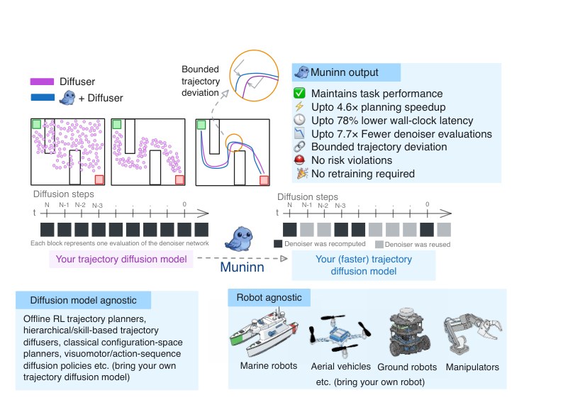
Fig. 1: High-level overview of Muninn applied to Diffuser. Diffuser recomputes the denoiser at every diffusion step, while Muninn wraps the same model and selectively reuses cached denoiser outputs at some steps, reducing compute while leaving the overall trajectory generation unchanged.
图 1:把 Muninn 用到 Diffuser 上的总体示意。Diffuser 在每一个扩散步都重新计算去噪器,而 Muninn 包装同一个模型,并在部分步骤上有选择地复用缓存的去噪器输出,从而减少计算,同时保持总体的轨迹生成过程不变。
A large body of work bypasses this issue by relying on model-based planning [41] and trajectory optimization [76, 54] with handcrafted costs and dynamics. These approaches can be fast [23], but tend to struggle when dynamics, human interactions, or multi-goal behaviors induce strongly multimodal solution sets [13, 28]. Diffusion-based planners address this [32] by learning complex trajectory distributions from data, yet they usually treat the denoiser as a black box and accept its inference cost as fixed. Efforts to reduce this cost follow several paths. One direction distills the diffusion process [59] into shallower networks [69] or coarse-to-fine samplers [68], but requires retraining for each architecture and sometimes each task. Another direction trains early-exit or policy networks [44] to decide when to stop denoising or which subnet to run; these methods can adapt computation per sample, but demand large-scale reinforcement learning or supervision [3] and tie the acceleration logic to a specific model.
大量工作绕开这一问题,转而依赖基于模型的规划 [41] 和带有手工设计代价与动力学的轨迹优化 [76, 54]。这些方法可以很快 [23],但当动力学、人机交互或多目标行为带来强多模态的解集合时,往往就会吃力 [13, 28]。基于扩散的规划器用从数据中学习复杂轨迹分布来应对这一点 [32],却通常把去噪器当成黑箱,并把它的推断代价当作固定的。降低这一代价的努力走了几条路。一条路线把扩散过程 [59] 蒸馏成更浅的网络 [69] 或由粗到细的采样器 [68],但需要对每种架构、有时还要对每个任务重新训练。另一条路线训练早退或策略网络 [44],以决定何时停止去噪或运行哪一个子网络;这些方法可以按样本调整计算量,但需要大规模强化学习或监督 [3],并把加速逻辑绑在特定模型上。
Recently, training-free accelerations [39, 27] have emerged that operate at inference time [4]. These approaches are attractive because they require no new data [36], works on existing architectures [7], and can deliver large wall-clock gains [72]. However, they are typically calibrated on perceptual or pixel-space metrics and developed for vision backbones. Little is known about how their approximation errors translate into trajectory deviations, and almost nothing is said about the consequences of those deviations for closed-loop control.
近来出现了在推理时运作的免训练加速 [39, 27, 4]。这类方法有吸引力,因为它们不需要新数据 [36],可用于已有架构 [7],并能带来可观的墙钟收益 [72]。不过,它们通常按感知或像素空间指标来校准,并且是为视觉骨干开发的。它们的近似误差如何转化为轨迹偏差,人们所知甚少;这些偏差对闭环控制意味着什么,更几乎没有被讨论。
We make two observations about diffusion-based planners: (i) every denoising step passes the current noisy trajectory and diffusion timestep through a relatively cheap input-processing stage to produce a representation that feeds the deeper network blocks. Changes in this representation across timesteps provide a natural, low-cost signal for how stable the trajectory is becoming, (ii) the sampler used to map denoiser outputs into new trajectories has a known analytic form: for a given schedule, we can write down exactly how a perturbation in the predicted noise at step changes the state at step . Taken together, these two facts suggest that the planner itself contains enough structure to estimate, for each step, how risky it would be to reuse a past denoiser output instead of recomputing a new one. These observations motivate the central idea of this work.
我们对基于扩散的规划器做两点观察:(i)每一步去噪都会把当前带噪轨迹和扩散时间步送进一个相对便宜的输入处理阶段,得到再送入更深网络块的表示。这一表示在时间步之间的变化,为轨迹正在变得多稳定提供了一个自然、低成本的信号;(ii)把去噪器输出映射成新轨迹的采样器具有已知的解析形式:对给定的时间表,我们可以精确写出第 步预测噪声上的扰动如何改变第 步的状态。合在一起,这两点说明规划器自身已经包含足够的结构,可以在每一步估计:复用过去的去噪器输出、而不是重新计算一个新输出,会有多大风险。这些观察引出了本工作的核心想法。
Statement of contributions: We introduce (i) Muninn[^1], a training-free wrapper for trajectory diffusion models that uses a cheap, timestep-wise probe of the internal representation to predict how much the final trajectory would change if a cached denoiser output were reused; (ii) a trajectory-level error budget that aggregates these predictions into decisions about when to reuse past denoiser outputs and when to recompute them, trading off planning speed against fidelity; and (iii) an evaluation on several diffusion-based planners across simulated and hardware navigation and manipulation benchmarks. We also release the code, dataset and models.
贡献说明:我们提出(i)Muninn[^1],一个面向轨迹扩散模型、无需训练的包装器,它用对内部表示的廉价、逐步探针,来预测若复用缓存的去噪器输出,最终轨迹会变化多少;(ii)一个轨迹级误差预算,把这些预测汇成何时复用、何时重算的决策,从而在规划速度与保真度之间权衡;(iii)在仿真和硬件上的导航与操作基准中,对若干基于扩散的规划器所做的评估。我们同时公开代码、数据集和模型。
1 “For Huginn I fear lest he come not home, / But for Muninn my care is more …”– Norse mythology. Muninn is Odin’s raven of memory. We borrow the name as a metaphor–relying on memory to move faster, while being careful not to stray far from the path we would have taken.
1 “For Huginn I fear lest he come not home, / But for Muninn my care is more …”– Norse mythology。Muninn 是奥丁那只象征记忆的乌鸦。我们借用这个名字作比喻——依靠记忆走得更快,同时小心不要偏离本来会走的那条路。
Note (scope). Diffusion planners span many architectures [74, 65]; we focus on state-space trajectory diffusion models that denoise future state or state–action sequences conditioned on observations and goals. Extending Muninn to other families mainly requires redefining the probe; the caching framework is unchanged, though the adaptation can be nontrivial.
范围说明。 扩散规划器覆盖许多架构 [74, 65];我们聚焦于状态空间轨迹扩散模型,它们在观测和目标的条件下,对未来状态或状态–动作序列做去噪。把 Muninn 扩展到其他家族,主要需要重新定义探针;缓存框架本身不变,尽管适配未必简单。
II. Related Work
II. 相关工作
Trajectory diffusion models: Early learning-based trajectory planners used imitation learning [50, 10] and variational generative models [25] to clone expert demonstrations. Conditional VAEs [26], normalizing flows [53], and graph latent models [19] capture diverse behaviors, but emit a single trajectory and rely on delicate training heuristics. Diffusion-based planners instead learn a denoising process over trajectories, achieving SOTA coverage of multimodal motions and have been applied to visual robot control [9], motion planning [21], and multi-agent behavior forecasting [75]. By sampling different noise realizations, these models naturally explore distinct homotopy classes [34] and avoid hand-crafted reward engineering. Yet standard samplers still require tens of denoising steps per plan [15], leading to second-level latencies and motivating recent work on accelerated trajectory diffusion [57].
轨迹扩散模型: 早期基于学习的轨迹规划器使用模仿学习 [50, 10] 和变分生成模型 [25] 来克隆专家示范。条件 VAE [26]、流模型 [53] 和图潜变量模型 [19] 可以刻画多样行为,但只发出一条轨迹,并依赖精细的训练启发式。基于扩散的规划器则学习轨迹上的去噪过程,在多模态运动覆盖上达到当时最好的水平,并已被用于视觉机器人控制 [9]、运动规划 [21] 和多智能体行为预测 [75]。通过采样不同的噪声实现,这些模型自然会探索不同的同伦类 [34],并避免手工设计奖励。然而标准采样器每条规划仍需要数十步去噪 [15],带来秒级延迟,也促使了近期关于加速轨迹扩散的工作 [57]。
Accelerating Diffusion via Model Design: In this vein, architectures compress the sampling chain while preserving multimodal coverage [58, 24]. One line of work distills multi-step samplers into shallow or one-step networks [52], or learns coarse-to-fine denoisers that jump directly to high-quality trajectories in a few iterations [16]. Other works bias the generative process with structured priors, trajectory libraries, or policy heads [14], so that sampling is guided toward task-feasible plans and fewer refinement steps are needed [18]. A complementary direction aggregates a set of diffusion rollouts into graphs, reusing evaluations across branches to reduce latency without sacrificing robustness [22]. These approaches demonstrate that careful parameterisation can shrink diffusion horizons, bringing trajectory diffusion closer to real-time operation [31, 55]. However, these accelerations still rely on sequential denoising, task-specific heuristics and typically operate by hard-coding new samplers or compressing the backbone network [49]. They degrade trajectory quality, require retraining for each architecture, and offer no guarantees on how the modified sampling process affects downstream control performance [42].
通过模型设计加速扩散: 沿着这条路线,一些架构在压缩采样链的同时保持多模态覆盖 [58, 24]。一条工作把多步采样器蒸馏成浅网络或单步网络 [52],或学习由粗到细的去噪器,用少数几次迭代直接跳到高质量轨迹 [16]。另一些工作用结构化先验、轨迹库或策略头来偏置生成过程 [14],从而把采样引向任务可行的规划,并减少所需的精炼步数 [18]。一条互补的路线把一组扩散滚动结果聚成图,在分支之间复用评估,以在不牺牲稳健性的前提下降低延迟 [22]。这些方法表明,仔细的参数化可以缩短扩散视界,使轨迹扩散更接近实时运行 [31, 55]。不过,这些加速仍然依赖顺序去噪和任务特定启发式,通常还要通过硬编码新采样器或压缩骨干网络来实现 [49]。它们会降低轨迹质量,需要为每种架构重新训练,并且对修改后的采样过程如何影响下游控制表现不提供保证 [42]。
Adaptive Inference and Early Exiting: Beyond architectural changes, a parallel line of work accelerates diffusion models via dynamic inference [12], using learned early-exit policies [60] or step-skipping heuristics [61]to reduce test-time compute. In diffusion models, such methods typically monitor simple signals along the sampling chain to decide when to stop, skip, or jump ahead in the denoising schedule [43, 37, 73]. Related approaches in sequence modeling and control reuse cached network outputs across time or across similar inputs, treating repeated evaluations as an optimization lever rather than changing the underlying architecture [30, 1]. These strategies are usually trained in a task-specific, data-driven fashion and lack explicit bounds on how shortcutting or cache reuse perturbs the final sample [8, 38]. They provide little formal guidance on how much an accelerated diffusion run can deviate from its full-compute counterpart, and offer no guarantees on the quality of the executed trajectory [5, 40].
自适应推断与早退: 在架构改动之外,另一条平行路线通过动态推断来加速扩散模型 [12],使用学到的早退策略 [60] 或跳步启发式 [61] 来减少测试时计算。在扩散模型中,这类方法通常沿采样链监测简单信号,以决定何时停止、跳过或在去噪时间表中向前跳 [43, 37, 73]。序列建模与控制中的相关方法则在时间上或在相似输入之间复用缓存的网络输出,把重复评估当成优化杠杆,而不是改动底层架构 [30, 1]。这些策略通常以任务特定、数据驱动的方式训练,对捷径或缓存复用如何扰动最终样本缺少显式界 [8, 38]。它们几乎不提供形式化指导,说明一次加速后的扩散运行相对全程计算会对齐到什么程度,也对执行轨迹的质量不提供保证 [5, 40]。
In contrast to prior works, we place Muninn at the intersection of trajectory diffusion and sampling-time acceleration, focusing on making existing trajectory planners fast enough without modifying or retraining their underlying networks.
与先前工作不同,我们把 Muninn 放在轨迹扩散和采样时加速的交叉处,重点是让已有的轨迹规划器足够快,而不修改或重训其底层网络。
III. Preliminaries and Challenges
III. 预备知识与挑战
A pretrained diffusion planner operates over trajectories and contexts via a fixed reverse-diffusion sampler: where is the denoiser and is a known sampler update (DDPM (Denoising Diffusion Probabilistic Models)/DDIM (Denoising Diffusion Implicit Models)-style; captures any sampler noise, with for deterministic samplers). Let be the resulting full-compute trajectory (evaluating at every step). Each denoiser call has cost , so a full planning call costs .
一个预训练的扩散规划器通过固定的反向扩散采样器,在轨迹 和上下文 上运作:,其中 是去噪器, 是已知的采样器更新(DDPM/DDIM 风格; 表示采样器噪声,对确定性采样器有 )。令 为由此得到的全程计算轨迹(每一步都评估 )。每次去噪器调用的代价为 ,因此一次完整规划调用的代价是 。
Challenges of caching in diffusion-based planners: The repeated denoising structure makes diffusion planners an appealing target for caching: the same network is invoked at every step, and consecutive timesteps often process very similar noisy trajectories. However, the same properties that make these models expressive, make safe caching surprisingly hard!
在基于扩散的规划器中做缓存的挑战: 反复去噪的结构使扩散规划器成为缓存的诱人对象:同一个网络在每一步被调用,相邻时间步又常常处理非常相似的带噪轨迹。可是,让这些模型具有表达力的那些性质,也让安全的缓存出乎意料地困难!
First, denoising is globally coupled over the horizon: each evaluation acts on the full trajectory , and the sampler mixes the predicted noise back into all time steps of , so a single approximation can bias the entire plan. Second, errors accumulate in a history-dependent way (see Fig. 2): reverse diffusion is iterative, so errors injected early are propagated and transformed by later updates; under nonlinear, contact-rich, or unstable dynamics, the same local denoiser error can have very different downstream effects depending on context and when it occurs. Third, control objectives are often discontinuous in trajectory space: small trajectory changes can flip outcomes from success to collision or constraint violation, so controlling only smooth surrogates can yield highly variable task impact.
首先,去噪在整个视界上是全局耦合的:每次评估都作用在整条轨迹 上,采样器又把预测噪声混回 的所有时间步,因此一次近似就可能偏置整条规划。其次,误差以依赖历史的方式累积(见图 2):反向扩散是迭代的,早先注入的误差会被后续更新传播和变换;在非线性、富接触或不稳定的动力学下,同样的局部去噪器误差会因上下文和出现时机不同,而对下游产生很不一样的影响。第三,控制目标在轨迹空间中常常是不连续的:轨迹上的小变化就可能把结果从成功翻成碰撞或约束违反,因此只控制平滑代理量,任务影响会高度可变。
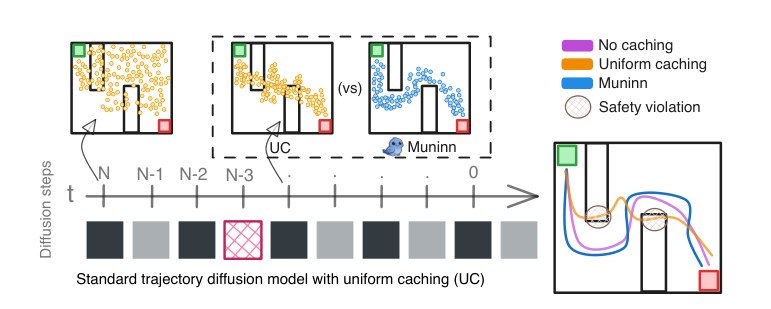
Fig. 2: Challenges in caching trajectory diffusion models. A mistaken reuse at one timestep (red) is not local: the reused output is mixed into all subsequent updates, causing errors to accumulate and shift the entire final trajectory.
图 2:在轨迹扩散模型中做缓存所面临的挑战。在某一个时间步上错误地复用(红色)并不是局部的:被复用的输出会混进此后所有更新,使误差累积并推动整条最终轨迹发生偏移。
Together, these effects create an all-or-nothing reuse regime: safe reuse requires confidence not only that the local approximation is small, but that its contribution remains acceptable after all subsequent sampler updates. Coarse strategies (e.g., fixed step skipping) oscillate between being overly conservative (limited speedup) and overly aggressive (hard-to-predict failures). Since practical diffusion planners vary in architecture, schedules, and conditioning, approaches that rely on retraining lose generality. This motivates caching mechanisms that (i) cheaply detect when reuse is risky, (ii) account for sampler-mediated error propagation, and (iii) expose interpretable knobs for trading compute against trajectory deviation.
这些效应合在一起,造成了一种非此即彼的复用局面:要安全复用,不仅需要确信局部近似足够小,还要确信它在所有后续采样器更新之后仍然可以接受。粗糙策略(例如固定跳步)会在过于保守(加速有限)和过于激进(难以预测的失败)之间摇摆。由于实际的扩散规划器在架构、时间表和条件化上各不相同,依赖重训的方法会失去通用性。这促使我们寻找这样的缓存机制:(i)能廉价地发现何时复用有风险,(ii)能计入由采样器介导的误差传播,并且(iii)提供可解释的旋钮,以便在计算量与轨迹偏差之间权衡。
IV. Muninn
Motivated by these challenges, Muninn is a training-free caching policy that, at each diffusion step, either recomputes or reuses a cached denoiser output to produce a lower-cost trajectory . It exposes two user-facing knobs: a deviation tolerance and risk level , and aims to minimize expected planning subject to .
受这些挑战推动,Muninn 是一种无需训练的缓存策略:在每一个扩散步,它要么重新计算 ,要么复用缓存的去噪器输出,以得到代价更低的轨迹 。它向用户露出两个旋钮:偏差容差 和风险水平 ,目标是在 的约束下,最小化期望规划代价。
A. Trajectory diffusion and sampler sensitivity
A. 轨迹扩散与采样器敏感性
We begin by making precise how local errors in the denoiser’s output at each diffusion step affect the final trajectory.
我们首先把每一步去噪器输出上的局部误差如何影响最终轨迹,说清楚。
Reverse diffusion as a paired process: Recall that is produced by evaluating the denoiser at every step. Caching policies modify this process by reusing denoiser outputs at selected timesteps instead of recomputing them. To isolate the effect of reuse, we analyze a paired run: the full and cached chains share the same initial sample and the sampler noise sequence , and differ only in the denoiser outputs . Let denote the cached trajectory at step and let be the noise prediction actually used at step (recomputed or reused). The cached chain evolves as . Muninn will choose by recomputing or by reusing a cached prediction.
作为成对过程的反向扩散: 回想 是通过在每一步评估去噪器得到的。缓存策略 会在选定的时间步复用去噪器输出,而不是重新计算,从而修改这一过程。为单独看清复用的影响,我们分析一次成对运行:全程链和缓存链共享同一个初始样本 和采样器噪声序列 ,差别只在去噪器输出 。令 表示第 步的缓存轨迹, 为该步实际使用的噪声预测(重算或复用)。缓存链按 演化。Muninn 将通过重算 ,或复用一个缓存预测,来选择 。
Error variables: We define two per-step errors: the trajectory drift and the denoiser mismatch , capturing divergence in trajectory space and in the noise prediction, respectively. Unless stated otherwise, denotes the Frobenius norm on . Our only assumption on the sampler is a local Lipschitz property:
误差变量: 我们定义两种逐步误差:轨迹漂移 ,以及去噪器失配 ,分别刻画轨迹空间和噪声预测上的分歧。除非另有说明, 表示 上的 Frobenius 范数。我们对采样器仅做局部 Lipschitz 假定:
Assumption 1(Sampler Lipschitzness).
假设 1(采样器 Lipschitz 性)。
For timestep , there exist nonnegative constants and such that, for any trajectories , noise predictions , and fixed sampler noise ,
对时间步 ,存在非负常数 和 ,使得对任意轨迹 、噪声预测 以及固定的采样器噪声 ,有
For DDPM/DDIM-style samplers, is affine in and , so and follow directly from the update coefficients. Conceptually, scales trajectory differences, while scales sensitivity to noise-prediction error. Applying Assumption 1 to the full-compute and cached updates at step gives
对 DDPM/DDIM 风格的采样器, 对 和 是仿射的,因此 和 可以直接由更新系数得出。概念上, 放缩轨迹差别,而 放缩对噪声预测误差的敏感性。把假设 1 应用到第 步的全程计算更新和缓存更新,得到
This recursion decomposes the trajectory error at step into a part inherited from the existing trajectory mismatch and a new contribution from the denoiser error .
这一递推把第 步的轨迹误差拆成两部分:从已有轨迹失配 继承下来的部分,以及来自去噪器误差 的新贡献。
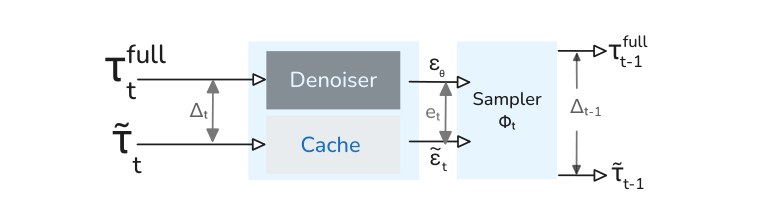
Fig. 3: Paired reverse-diffusion step. is the denoiser error from reusing and is the induced trajectory mismatch; a Lipschitz bound splits into propagated mismatch and injected error.
图 3:成对的反向扩散步骤。 是复用 带来的去噪器误差, 是由此引起的轨迹失配;一个 Lipschitz 界把 拆成传播而来的失配和新注入的误差。
Unrolling the recursion: Both processes are initialized from the same noisy trajectory, so . Repeatedly applying the local bound (1) from down to yields a closed-form bound on . For we have . Continuing, a simple induction shows,
展开递推: 两条过程从同一条带噪轨迹初始化,因此 。从 一直到 反复应用局部界(1),就得到 的闭式界。在 时,有 。继续下去,一个简单的归纳表明,
Defining the pathwise sensitivity coefficients, , we can rewrite (2) at compactly as
定义路径上的敏感性系数 ,我们可以把(2)在 处紧凑地改写为
Each step’s denoiser error contributes additively to the final trajectory deviation, weighted by , capturing how strongly errors at are amplified through subsequent diffusion updates.
每一步的去噪器误差 都以 为权重,加性地贡献到最终轨迹偏差,刻画第 步的误差会通过后续扩散更新被放大到何种程度。
From norm difference to trajectory deviation: The guarantee in our problem statement is expressed in terms of a user-chosen trajectory metric . We assume that is Lipschitz-equivalent to the norm in the sense that:
从范数差到轨迹偏差: 问题陈述中的保证,是用用户选定的轨迹度量 来表达的。我们假定 在下述意义上与范数 Lipschitz 等价:
Assumption 2(Metric compatibility).
假设 2(度量相容性)。
There exists a constant such that for all , .
存在常数 ,使得对所有 ,有 。
Combining Assumption 2 with (3) yields:
把假设 2 与(3)结合,得到:
Equation (4) is the key trajectory deviation bound. It exposes that an error injected at step is scaled by , which depends on all later sampler sensitivities . Early steps can therefore have a larger impact than late steps. In our experiments we use , with .
式(4)是关键的轨迹偏差界。它表明,在第 步注入的误差 会被 放缩,而 依赖于此后所有采样器敏感性 。因此较早的步骤可能比较晚的步骤影响更大。实验中我们使用 ,并取 。
We define the per-step trajectory cost associated with a as . Then (4) simply states that the total trajectory deviation is bounded by the sum of per-step costs,
我们把与 相应的逐步轨迹代价定义为 。于是(4)只不过是说,总轨迹偏差被逐步代价之和所界定,
Muninn uses (5) as a budget rule: if each reuse step has a high-probability upper bound on and the summed bounds stay within , then the final cached trajectory remains within of the full-compute one with the same high probability.
Muninn 把(5)当作预算规则:若每一步复用都对 有一个高概率上界,且这些上界之和保持在 之内,那么最终的缓存轨迹就会以同样的高概率,保持在全程计算轨迹的 距离之内。
Now, the challenge is that, during deployment, the actual denoiser error is unknown for a reuse decision.
现在的困难是,在部署时,对一次复用决策而言,实际的去噪器误差 是未知的。
B. Probe features and per-step error scores
B. 探针特征与逐步误差分数
The sensitivity bound (4) quantifies how costly a step- error would be, but not how large that error would be under reuse. In order to do that, we introduce (i) a lightweight probe , and (ii) per-step score . Fig. 4 summarizes this subsection.
敏感性界(4)量化的是第 步误差 会有多“贵”,而不是复用时这个误差会有多大。为回答后者,我们引入(i)一个轻量探针 ,以及(ii)逐步分数 。图 4 概括了这一小节。
Probe features: At step , the denoiser is evaluated on the current noisy and context . In almost all modern architectures, this evaluation can be decomposed into: (i) an input processing or “stem” stage that maps into an intermediate representation , and (ii) a deeper, expensive “core” that refines into the final noise prediction .
探针特征: 在第 步,去噪器 在当前带噪 和上下文 上被评估。在几乎所有现代架构中,这次评估可以分解为:(i)一个输入处理或“茎干”阶段,把 映成中间表示 ;(ii)一个更深、更贵的“核心”,把 精炼成最终噪声预测 。
We exploit this decomposition by defining a probe feature that depends only on the cheaper part of the computation and is therefore inexpensive to compute at every step.
我们利用这一分解,定义一个只依赖较便宜计算部分的探针特征 ,因而在每一步计算它都不昂贵。
Formally, we posit a probe function and define . We require to satisfy two design goals: (i) The cost of evaluating at a single step should be negligible compared to a full pass through . (ii) Architecture-agnostic: Any trajectory diffusion model provides an intermediate representation between its input and its final noise prediction. By defining in terms of this representation, we ensure that Muninn can be applied to a wide range of state-space diffusion planners without architectural changes.
形式上,我们设定探针函数 ,并定义 。我们要求 满足两个设计目标:(i)在单步上评估 的代价,相对完整穿过 应当可以忽略;(ii)与架构无关:任何轨迹扩散模型都在输入和最终噪声预测之间提供中间表示。把 定义在这一表示上,就能保证 Muninn 可以应用到广泛的状态空间扩散规划器,而不改架构。
Per-step error scores from probe dynamics: Intuitively, reuse is safe when the denoiser’s output would not have changed much when recomputed. We expect this to happen when has stabilized: if the probe at step is similar to the nearby steps, the model is likely to produce similar noise predictions, and using a cached output should incur a small error .
由探针动态得到的逐步误差分数: 直观上,当去噪器的输出即便重算也不会有太大变化时,复用是安全的。我们预期这会发生在 已经稳定的时候:若第 步的探针与邻近步骤相似,模型就很可能产生相似的噪声预测,使用缓存输出应只带来较小的误差 。
To capture this intuition, Muninn maps the sequence of probe features into a scalar error score at each step . This score should be: (i) cheap to compute from probe features we have, (ii) monotonically informative in the sense that smaller scores tend to correspond to smaller denoiser errors.
为抓住这一直观,Muninn 把探针特征序列 映成每一步 上的标量误差分数 。这个分数应当:(i)从已有探针特征出发计算起来便宜;(ii)在单调的意义上有信息量,即较小的分数往往对应较小的去噪器误差。
Since reverse diffusion runs from to , the reuse decision at step can use both the current probe and the previously computed . A effective choice of score is the magnitude of the probe change between these two steps:
由于反向扩散从 跑到 ,第 步的复用决策既可以用当前探针 ,也可以用先前算好的 。一个有效的分数选择,是这两步之间探针变化的幅度:
where . This design reflects two intuitions: (i) when stabilizes, changes slowly and the denoiser output changes little, so reuse yields small ; (ii) as sensitivity varies with timestep (via ), calibrating score-to-error bounds per adapts reuse decisions to high-impact regions of the diffusion chain.
其中 。这一设计反映两点直观:(i)当 稳定时, 变化缓慢,去噪器输出也变化很小,因而复用带来的 较小;(ii)敏感性随时间步变化(通过 ),按 校准分数到误差的界,就能让复用决策适应扩散链中影响更大的区域。
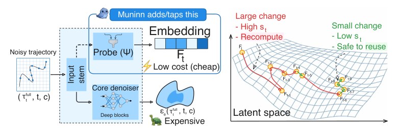
Fig. 4: Probe features and per-step error scores. (Left) A denoiser evaluation decomposes into a cheap stem and an expensive core; Muninn runs only the stem to compute a lightweight probe. (Right) Large step-to-step changes () trigger recomputation, while small indicate stability and make reuse safe.
图 4:探针特征与逐步误差分数。(左)一次去噪器评估被分解为廉价的茎干和昂贵的核心;Muninn 只运行茎干来计算轻量探针。(右)步与步之间的大变化()会触发重算,而小的 表明已经稳定,复用是安全的。
C. Conformal calibration of reuse error
C. 复用误差的共形校准
Section IV-A bounds trajectory deviation by a sum of per-step costs. To use this bound online, Muninn needs a high-probability upper bound on the (unknown) reuse error at each step. We now show how to obtain these bounds.
第 IV-A 节用逐步代价之和来界定轨迹偏差。要在线使用这个界,Muninn 需要在每一步对(未知的)复用误差 有一个高概率上界。我们接下来说明如何得到这些界。
Calibration data: Recall that the trajectory deviation bound (4) depends only on its magnitude . We therefore define the scalar error and aim to predict from the score introduced in (6).
校准数据: 回想轨迹偏差界(4)只依赖于其幅度 。因此我们定义标量误差 ,并希望从(6)中引入的分数 来预测 。
At deployment, is the noise prediction actually reused by Muninn at step , which depends on the entire history of recompute vs. reuse decisions. For calibration, we fix a policy-agnostic reuse rule that defines a potential reuse output at every step, independent of the budget. We define a deterministic map that, specifies which earlier denoiser output would be reused if we chose to reuse at . For e.g., we can always reuse the prediction from the previous step that evaluated .
在部署时, 是 Muninn 在第 步实际复用的噪声预测,它依赖于此前全部重算与复用决策的历史。为了校准,我们固定一条与策略无关的复用规则,在每一步定义一个潜在的复用输出,而不依赖预算。我们定义一个确定性映射,指明若在 选择复用,会复用更早哪一次去噪器输出。例如,我们可以总是复用上一次评估 的那一步预测。
Given this potential reuse rule, we build a calibration set by running the full-compute chain alongside a paired ghost reuse chain on i.i.d. episodes from the deployment distribution. For each episode and each , we record (i) the probe-based score computed from the ghost chain, and (ii) the corresponding potential reuse error magnitude . The resulting calibration dataset is the collection of score–error pairs , where is the set of timesteps at which reuse is allowed. Appendix E and Figure 5 provide the full construction details.
有了这条潜在复用规则,我们通过在来自部署分布的 个独立同分布回合上,把全程计算链与一条成对的幽灵复用链一起运行,来构建校准集。对每个回合 和每个 ,我们记录(i)由幽灵链算出的基于探针的分数 ,以及(ii)相应的潜在复用误差幅度 。得到的校准数据集是分数–误差对的集合 ,其中 是允许复用的时间步集合。附录 E 和图 5 给出完整的构造细节。
Since the reuse pattern is fixed and independent of , we can view each as a draw from a common, unknown joint distribution over scores and potential reuse errors induced by the base planner and environment. Under the exchangeability assumption—calibration and deployment episodes are sampled i.i.d. from —this is the setting where conformal prediction provides finite-sample coverage guarantees.
由于复用模式是固定的,且与 独立,我们可以把每一对 看作来自由基座规划器和环境诱导的、未知的分数与潜在复用误差联合分布的一次抽取。在可交换假定下——校准回合和部署回合都从 独立同分布抽样——这正是共形预测提供有限样本覆盖保证的设定。
Split-conformal regression: Given , we construct a function that maps each score to a high-probability upper bound on the corresponding potential reuse error . Concretely, we fit a regression model on a training split of and apply split conformal prediction on a held-out split to obtain an additive residual quantile . This results in the bound ; Appendix E provides the full construction.
分裂共形回归: 给定 ,我们构造函数 ,把每个分数 映射为相应潜在复用误差 的高概率上界。具体来说,我们在 的训练划分上拟合回归模型 ,再在留出划分上做分裂共形预测,得到加性残差分位数 。由此得到界 ;附录 E 给出完整构造。
By split conformal prediction, assuming exchangeability between calibration and deployment, we obtain per-step coverage: for a new step with score and potential reuse error ,
根据分裂共形预测,在校准与部署可交换的假定下,我们得到逐步覆盖:对一个分数为 、潜在复用误差为 的新步骤,
This guarantee is distribution-free: it holds for any joint distribution of as long as calibration and deployment samples are exchangeable. The regressor only tightens ; even if is misspecified, (7) holds by construction.
这一保证是与分布无关的:只要校准样本与部署样本可交换,它对 的任何联合分布都成立。回归器 只是让 更紧;即便 被设错,(7)也由构造保证成立。
From per-step coverage to global risk: The per-step coverage (7) applies to the latent potential reuse error at any timestep . Combining with the upper bound gives, for any step , . If we define the upper-bounded per-step cost at score as then with probability at least ,
从逐步覆盖到全局风险: 逐步覆盖(7)适用于任意时间步 上的潜在复用误差 。把 与上界 结合起来,对任意步骤 ,只要 ,就有 。若把分数 处的上界逐步代价定义为 ,则至少以概率 ,
Crucially, the event depends only on the underlying data-generating process and the calibration procedure; it is independent of the caching policy we will deploy later.
关键在于,事件 只依赖于底层数据生成过程和校准程序;它与我们稍后将部署的缓存策略无关。
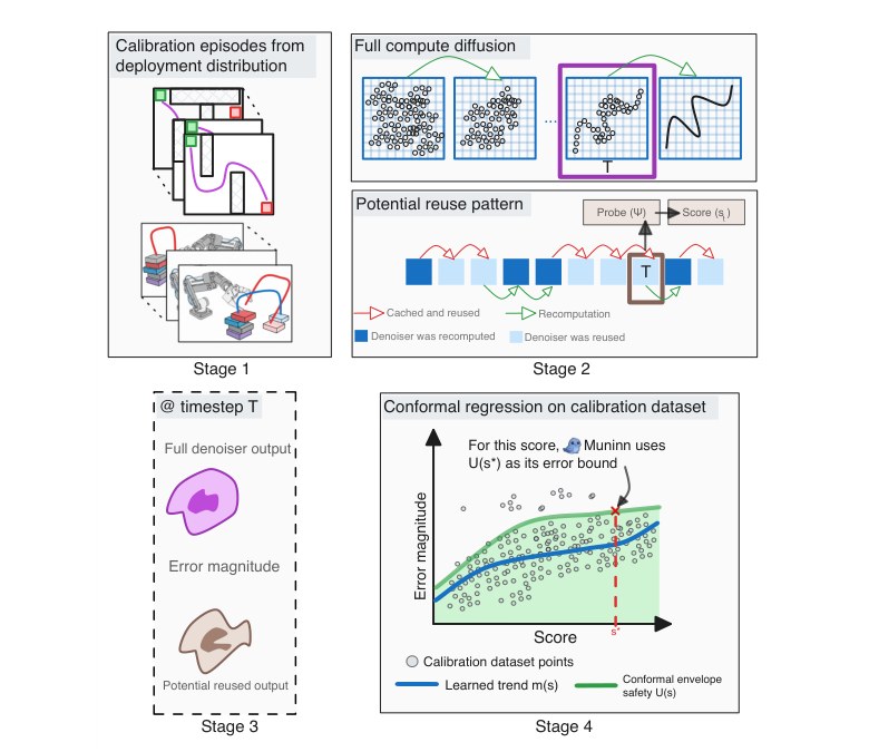
Fig. 5: (Stages 1–3) From offline rollouts, we build a calibration set of score–error pairs by running the full planner with a ghost reuse chain. (Stage 4) A regressor models the typical score–error relationship, and split conformal prediction yields . At test time, Muninn maps each score to , converts it to a trajectory-level cost, and spends it from the budget.
图 5:(阶段 1–3)从离线滚动中,我们通过运行带有“幽灵”复用链的完整规划器,构建分数–误差对校准集。(阶段 4)回归器 刻画典型的分数–误差关系,分裂共形预测给出 。测试时,Muninn 把每个分数映射为 ,再把它换成轨迹级代价,并从预算中花掉。
D. Muninn caching policy
D. Muninn 的缓存策略
Muninn uses the per-step bounds to decide online, per sample, whether to reuse or recompute. The idea is to interpret (5) as a budget constraint: user specifies a maximum allowable which is spent across reverse-diffusion steps.
Muninn 用逐步界 在线地、按样本决定是复用还是重算。想法是把(5)理解成预算约束:用户指定一个最大允许的 ,再把它花在反向扩散的各步上。
Budgeted reuse rule: At deployment time, the true error at is unknown. Let denote the set of timesteps where reuse is permitted. We maintain a remaining budget and, for clarity, we summarize the algorithm below.
带预算的复用规则: 部署时,第 步的真实误差 是未知的。令 表示允许复用的时间步集合。我们维护剩余预算 ,并为清楚起见,把算法概括如下。
Algorithm 1 Muninn caching policy for one planning call
1: Sample initial noisy trajectory .
2: Initialize: (i) , (ii) .
3: for do
4: Compute probe .
5: if then
6: Retrieve previous probe // stored at step .
7: Compute score
8: Compute upper-bounded cost .
9: end if
10: if or or ( **and** ) then
11: Recompute:
12:
13: Update cache with as most recent recompute.
14:
15: else
16: Reuse:
17: Set to the cached denoiser output specified by the potential reuse rule.
18:
19: end if
20: Apply sampler update:
21: Store // for use at step .
22: end for
23: return
算法 1 一次规划调用中的 Muninn 缓存策略
1: 从 采样初始带噪轨迹 。
2: 初始化:(i),(ii)。
3: for do
4: 计算探针 。
5: if then
6: 取回上一探针 // 在第 步存下。
7: 计算分数
8: 计算上界代价 。
9: end if
10: if or or( **and** )then
11: 重算:
12:
13: 用 更新缓存,作为最近一次重算。
14:
15: else
16: 复用:
17: 按潜在复用规则,把 设为缓存的去噪器输出。
18:
19: end if
20: 应用采样器更新:
21: 存储 // 供第 步使用。
22: end for
23: return
This policy is: (i) budget-safe by construction: enforcing ensures that the sum of upper-bounded costs over reuse steps satisfies ; (ii) sample-adaptive: reuse locations and counts depend on the realized scores (and thus on the context, noise, and trajectory).
这一策略:(i)由构造保证预算安全:强制 ,就保证复用步上上界代价之和满足 ;(ii)对样本自适应:复用位置和次数依赖于实现出来的分数 (因而也依赖于上下文、噪声和轨迹)。
Global risk guarantee: Under the conformal calibration guarantee (7), for each in a planning episode we have . Define the failure event at step as . By construction of ,
全局风险保证: 在共形校准保证(7)下,规划回合中的每一步 都满足 。把第 步的失败事件定义为 。由 的构造,
Recall that is defined w.r.t. the potential reuse rule, and at reuse, Muninn uses the same rule to choose which cached output to apply. Thus, whenever Muninn reuses at step , the realized denoiser error magnitude coincides with the latent potential reuse error for that step.
回想 是相对于潜在复用规则定义的,而在复用时,Muninn 用同一条规则来选择应用哪一个缓存输出。因此,只要 Muninn 在第 步复用,实现出来的去噪器误差幅度 就与该步潜在的复用误差 重合。
Now consider a single planning episode. If none of the failure events occur at any timestep in , then for all reuse steps we have , and thus the total trajectory deviation satisfies
现在考虑一次规划回合。若 中任何时间步都没有发生失败事件 ,则对所有复用步 都有 ,从而总轨迹偏差满足
Therefore, the only way for the trajectory deviation to exceed is if at least one failure event occurs: Taking probabilities and applying a union bound over timesteps yields
因此,轨迹偏差要超过 ,唯一的途径是至少发生一次失败事件: 取概率并对时间步应用并界,得到
If we choose , then (11) simplifies to
若取 ,则(11)简化为
which is exactly the risk guarantee from the problem statement.
而这正是问题陈述中的风险保证。
This guarantee does not require timestep independence: it follows from the per-step bounds (9) and a union bound. It holds for any adaptive reuse set , provided the reuse rule used to define in calibration matches the rule used at deployment.
这一保证并不要求各时间步独立:它由逐步界(9)和一个并界得出。它对任意自适应复用集合 都成立,只要校准中用来定义 的复用规则与部署时使用的规则一致。
E. Practical considerations and engineering choices
E. 实际考虑与工程选择
In practice, Muninn is implemented with a few simple engineering choices: (i) forbidden regions—we disallow reuse in a short prefix (large , highly noisy and sensitivity-amplifying) and suffix (small , where small changes in can directly affect executed motion); (ii) batched sampling—when multiple trajectories are denoised in parallel, we maintain an independent remaining budget per trajectory and apply the same reuse rule independently, so the guarantee (7) and bound (12) apply per trajectory; (iii) model instantiations—for Transformer trajectory denoisers we take as a short prefix of attention/MLP blocks and mean-pool tokens to obtain , while for MLP denoisers we use the penultimate hidden layer as , in all cases computing before the reuse decision at step and making them available during both calibration (to label ) and deployment (when is unknown).
实践中,Muninn 用几项简单的工程选择来实现:(i)禁止区域——我们不允许在一小段前缀( 很大,噪声高且敏感性被放大)和后缀( 很小,此时 的微小变化会直接作用于执行运动)上复用;(ii)批量采样——当多条轨迹并行去噪时,我们为每条轨迹维护独立的剩余预算 ,并独立应用同一条复用规则,因而保证(7)和界(12)对每条轨迹分别成立;(iii)模型实例化——对 Transformer 轨迹去噪器,我们把 取成注意力/MLP 块的一小段前缀,并对 token 做均值池化得到 ;对 MLP 去噪器,则用倒数第二层隐层作为 。在所有情形下,都在第 步做出复用决策之前计算 ,并在校准(用来给 贴标签)和部署(此时 未知)中都提供这些量。
V. Experiments
V. 实验
We evaluate Muninn on two trajectory-diffusion families covering the dominant uses of diffusion in robotics.
我们在两类轨迹扩散家族上评估 Muninn,它们覆盖了扩散在机器人学中的主要用法。
Trajectory diffusion planners (offline RL and motion planning) [6, 51, 21, 2, 62, 29, 35, 48] use diffusion as a planner over full state-action or configuration-space trajectories, implemented as an iterative reverse-diffusion process (optionally with guidance).
轨迹扩散规划器(离线强化学习和运动规划)[6, 51, 21, 2, 62, 29, 35, 48] 把扩散当作对完整状态–动作或构型空间轨迹的规划器,实现为迭代反向扩散过程(可选地带有引导)。
Diffusion policies (imitation and visuomotor control) [9, 71] use diffusion as a policy that generates short-horizon action or pose segments, conditioned on high-dimensional observations, and executed repeatedly in a receding-horizon control loop.
扩散策略(模仿和视觉运动控制)[9, 71] 把扩散当作策略,生成短时域的动作或位姿片段,以高维观测为条件,并在滚动时域控制回路中反复执行。
A. Quantitative Results: Simulation and Benchmarks
A. 定量结果:仿真与基准
We evaluate Muninn on trajectory centric benchmarks and report standard metrics as defined in the prior literature for each benchmark. See Appendix A for details on the environments, datasets, training, and metrics (Appendix C). All experiments are run on an NVIDIA A10 GPU (24GB VRAM) and averaged on 150 previously unseen episodes.
我们在以轨迹为中心的基准上评估 Muninn,并按各基准既有文献中定义的标准指标报告结果。环境、数据集、训练和指标的细节见附录 A(附录 C)。全部实验在一块 NVIDIA A10 GPU(24GB 显存)上运行,并在 150 个此前未见过的回合上取平均。
Offline RL / trajectory planning. We first consider the D4RL offline RL suite [11] for continuous control, where models act as trajectory optimizers/conditional policies over state-action.
离线强化学习 / 轨迹规划。我们首先考虑用于连续控制的 D4RL 离线强化学习套件 [11],其中模型充当状态–动作上的轨迹优化器 / 条件策略。
TABLE I: Offline RL and trajectory planning. Task metric is the benchmark metric (D4RL normalized score for D4RL tasks; success rate for Kuka stacking). is the trajectory deviation metric used for risk accounting and .
| Benchmark | Model | Task metr. Full | Task metr. + | Latency Full | Latency + | #Evals/t Full | #Evals/t + | ||
|---|---|---|---|---|---|---|---|---|---|
| MuJoCo locomotion (D4RL) | |||||||||
| HalfCheetah | Diffuser [21] | 59.3 | 58.8 | 580 | 145 | 100 | 17.0 | 0.056 | 0.045 |
| Dec. Diff. [2] | 62.9 | 61.9 | 116 | 40 | 20 | 5.4 | 0.042 | 0.038 | |
| Diff.-QL [62] | 63.7 | 63.6 | 20 | 10 | 10 | 4.4 | 0.030 | 0.028 | |
| AdaptDiff[29] | 59.6 | 59.5 | 353 | 101 | 60 | 12.4 | 0.050 | 0.041 | |
| Hopper | Diffuser [21] | 65.1 | 64.7 | 523 | 138 | 100 | 18.0 | 0.058 | 0.046 |
| Dec. Diff. [2] | 70.6 | 69.8 | 105 | 39 | 20 | 6.0 | 0.045 | 0.040 | |
| Diff.-QL [62] | 75.7 | 75.6 | 20 | 11 | 10 | 4.7 | 0.032 | 0.030 | |
| AdaptDiff[29] | 63.8 | 63.6 | 310 | 97 | 60 | 14.2 | 0.052 | 0.043 | |
| Walker2d | Diffuser [21] | 77.8 | 77.2 | 783 | 224 | 100 | 20.6 | 0.062 | 0.048 |
| Dec. Diff. [2] | 84.0 | 83.7 | 157 | 63 | 20 | 6.7 | 0.048 | 0.042 | |
| Diff.-QL [62] | 80.8 | 80.7 | 25 | 14 | 25 | 12.7 | 0.034 | 0.032 | |
| AdaptDiff[29] | 83.3 | 83.0 | 403 | 119 | 60 | 12.9 | 0.057 | 0.045 | |
| Goal-reaching navigation (D4RL) | |||||||||
| Maze2D | Diffuser [21] | 119.5 | 119.0 | 733 | 175 | 100 | 15.3 | 0.065 | 0.047 |
| Dec. Diff. [2] | 130.8 | 129.6 | 147 | 46 | 20 | 4.7 | 0.055 | 0.044 | |
| Diff.-QL [62] | 105.6 | 104.8 | 25 | 12 | 10 | 4.2 | 0.040 | 0.035 | |
| AdaptDiff[29] | 144.3 | 143.9 | 347 | 99 | 60 | 12.4 | 0.060 | 0.046 | |
| CompDiff[35] | 160.2 | 159.2 | 1100 | 275 | 150 | 25.0 | 0.070 | 0.049 | |
| AntMaze | Diffuser [21] | 58.7 | 58.3 | 950 | 207 | 100 | 13.0 | 0.072 | 0.049 |
| Dec. Diff. [2] | 72.2 | 71.8 | 190 | 53 | 20 | 4.0 | 0.060 | 0.046 | |
| Diff.-QL [62] | 59.6 | 59.4 | 25 | 10 | 25 | 8.8 | 0.045 | 0.038 | |
| AdaptDiff[29] | 63.0 | 62.7 | 550 | 145 | 60 | 10.9 | 0.065 | 0.047 | |
| CompDiff[35] | 75.9 | 74.5 | 1400 | 342 | 150 | 24.0 | 0.075 | 0.049 | |
| Long-horizon manipulation (D4RL) | |||||||||
| FrankaKitchen | Diffuser [21] | 53.4 | 53.0 | 800 | 235 | 100 | 21.6 | 0.058 | 0.045 |
| Dec. Diff. [2] | 55.0 | 54.9 | 160 | 62 | 20 | 6.3 | 0.045 | 0.040 | |
| AdaptDiff[29] | 58.1 | 57.7 | 450 | 167 | 60 | 18.0 | 0.050 | 0.042 | |
| Robot block stacking (Kuka) | |||||||||
| Kuka stacking | Diffuser [21] | 52.3 | 51.8 | 1200 | 400 | 100 | 25.9 | 0.055 | 0.044 |
| Dec. Diff. [2] | 60.4 | 60.0 | 240 | 100 | 20 | 7.0 | 0.045 | 0.040 |
表 I:离线强化学习和轨迹规划。 任务指标为各基准采用的指标(D4RL 任务用 D4RL 归一化分数;Kuka 堆叠用成功率)。 是用于风险核算的轨迹偏差度量,。
| 基准 | 模型 | 任务指标 Full | 任务指标 + | 延迟 Full | 延迟 + | 评估次数/轨迹 Full | 评估次数/轨迹 + | ||
|---|---|---|---|---|---|---|---|---|---|
| MuJoCo 运动(D4RL) | |||||||||
| HalfCheetah | Diffuser [21] | 59.3 | 58.8 | 580 | 145 | 100 | 17.0 | 0.056 | 0.045 |
| Dec. Diff. [2] | 62.9 | 61.9 | 116 | 40 | 20 | 5.4 | 0.042 | 0.038 | |
| Diff.-QL [62] | 63.7 | 63.6 | 20 | 10 | 10 | 4.4 | 0.030 | 0.028 | |
| AdaptDiff[29] | 59.6 | 59.5 | 353 | 101 | 60 | 12.4 | 0.050 | 0.041 | |
| Hopper | Diffuser [21] | 65.1 | 64.7 | 523 | 138 | 100 | 18.0 | 0.058 | 0.046 |
| Dec. Diff. [2] | 70.6 | 69.8 | 105 | 39 | 20 | 6.0 | 0.045 | 0.040 | |
| Diff.-QL [62] | 75.7 | 75.6 | 20 | 11 | 10 | 4.7 | 0.032 | 0.030 | |
| AdaptDiff[29] | 63.8 | 63.6 | 310 | 97 | 60 | 14.2 | 0.052 | 0.043 | |
| Walker2d | Diffuser [21] | 77.8 | 77.2 | 783 | 224 | 100 | 20.6 | 0.062 | 0.048 |
| Dec. Diff. [2] | 84.0 | 83.7 | 157 | 63 | 20 | 6.7 | 0.048 | 0.042 | |
| Diff.-QL [62] | 80.8 | 80.7 | 25 | 14 | 25 | 12.7 | 0.034 | 0.032 | |
| AdaptDiff[29] | 83.3 | 83.0 | 403 | 119 | 60 | 12.9 | 0.057 | 0.045 | |
| 目标到达导航(D4RL) | |||||||||
| Maze2D | Diffuser [21] | 119.5 | 119.0 | 733 | 175 | 100 | 15.3 | 0.065 | 0.047 |
| Dec. Diff. [2] | 130.8 | 129.6 | 147 | 46 | 20 | 4.7 | 0.055 | 0.044 | |
| Diff.-QL [62] | 105.6 | 104.8 | 25 | 12 | 10 | 4.2 | 0.040 | 0.035 | |
| AdaptDiff[29] | 144.3 | 143.9 | 347 | 99 | 60 | 12.4 | 0.060 | 0.046 | |
| CompDiff[35] | 160.2 | 159.2 | 1100 | 275 | 150 | 25.0 | 0.070 | 0.049 | |
| AntMaze | Diffuser [21] | 58.7 | 58.3 | 950 | 207 | 100 | 13.0 | 0.072 | 0.049 |
| Dec. Diff. [2] | 72.2 | 71.8 | 190 | 53 | 20 | 4.0 | 0.060 | 0.046 | |
| Diff.-QL [62] | 59.6 | 59.4 | 25 | 10 | 25 | 8.8 | 0.045 | 0.038 | |
| AdaptDiff[29] | 63.0 | 62.7 | 550 | 145 | 60 | 10.9 | 0.065 | 0.047 | |
| CompDiff[35] | 75.9 | 74.5 | 1400 | 342 | 150 | 24.0 | 0.075 | 0.049 | |
| 长时域操作(D4RL) | |||||||||
| FrankaKitchen | Diffuser [21] | 53.4 | 53.0 | 800 | 235 | 100 | 21.6 | 0.058 | 0.045 |
| Dec. Diff. [2] | 55.0 | 54.9 | 160 | 62 | 20 | 6.3 | 0.045 | 0.040 | |
| AdaptDiff[29] | 58.1 | 57.7 | 450 | 167 | 60 | 18.0 | 0.050 | 0.042 | |
| 机器人积木堆叠(Kuka) | |||||||||
| Kuka stacking | Diffuser [21] | 52.3 | 51.8 | 1200 | 400 | 100 | 25.9 | 0.055 | 0.044 |
| Dec. Diff. [2] | 60.4 | 60.0 | 240 | 100 | 20 | 7.0 | 0.045 | 0.040 |
Motion planning in configuration space. We then test Muninn on classical motion planning problems where trajectories are represented in joint space rather than as RL episodes.
构型空间中的运动规划。我们随后在经典运动规划问题上测试 Muninn,这些轨迹在关节空间中表示,而不是作为强化学习回合。
TABLE II: Configuration-space motion planning. Scenarios correspond to increasing clutter/difficulty under the EDMP [51] evaluation protocol. Collision/violation includes obstacle collisions and any hard constraint violations.
| Scen. | Model | Success (%) Full | Success (%) + | Collis. (%) Full | Collis. (%) + | Lat. (ms) Full | Lat. (ms) + | ||
|---|---|---|---|---|---|---|---|---|---|
| Arm planning in clutter | easy | MPD [6] | 99.0 | 98.8 | 1.0 | 1.2 | 180 | 120 | 0.040 |
| EDMP[51] | 99.5 | 99.4 | 0.5 | 0.6 | 120 | 92 | 0.035 | ||
| med. | MPD [6] | 94.0 | 93.5 | 6.0 | 6.4 | 200 | 118 | 0.045 | |
| EDMP[51] | 96.5 | 96.2 | 3.5 | 3.7 | 135 | 95 | 0.040 | ||
| hard | MPD [6] | 82.0 | 81.2 | 18.0 | 18.8 | 230 | 121 | 0.048 | |
| EDMP[51] | 88.0 | 87.5 | 12.0 | 12.4 | 160 | 107 | 0.044 |
表 II:构型空间运动规划。 场景对应 EDMP [51] 评估协议下逐渐增加的杂乱程度 / 难度。碰撞 / 违反包括障碍碰撞以及任何硬约束违反。
| 场景 | 模型 | 成功率(%) Full | 成功率(%) + | 碰撞(%) Full | 碰撞(%) + | 延迟(毫秒) Full | 延迟(毫秒) + | ||
|---|---|---|---|---|---|---|---|---|---|
| 杂乱中的手臂规划 | easy | MPD [6] | 99.0 | 98.8 | 1.0 | 1.2 | 180 | 120 | 0.040 |
| EDMP[51] | 99.5 | 99.4 | 0.5 | 0.6 | 120 | 92 | 0.035 | ||
| med. | MPD [6] | 94.0 | 93.5 | 6.0 | 6.4 | 200 | 118 | 0.045 | |
| EDMP[51] | 96.5 | 96.2 | 3.5 | 3.7 | 135 | 95 | 0.040 | ||
| hard | MPD [6] | 82.0 | 81.2 | 18.0 | 18.8 | 230 | 121 | 0.048 | |
| EDMP[51] | 88.0 | 87.5 | 12.0 | 12.4 | 160 | 107 | 0.044 |
Visuomotor imitation and manipulation. Finally, we evaluate Muninn on visuomotor policy diffusers that generate pose trajectories conditioned on images (2D) or 3D observations.
视觉运动模仿与操作。最后,我们在视觉运动策略扩散器上评估 Muninn,它们以图像(二维)或三维观测为条件生成位姿轨迹。
TABLE III: Visuomotor imitation and manipulation. Latency is measured per policy inference/control call. is defined on the trajectory segment.
| Benchmark/Metric | RLBench [20] Reach Target Diff. Policy [9] | Meta-World[70] pick-place-v2 Diff. Policy [9] | DP3 Pour DP3 [71] | |
|---|---|---|---|---|
| Success (%) | Full | 99.0 | 92.0 | 98.0 |
| + | 98.8 | 91.5 | 97.6 | |
| Latency (ms) | Full | 25 | 30 | 45 |
| + | 15 | 18 | 27 | |
| 0.035 | 0.040 | 0.038 | ||
| 0.040 | 0.045 | 0.043 |
表 III:视觉运动模仿与操作。 延迟按每次策略推理 / 控制调用测量。 定义在轨迹片段上。
| 基准 / 指标 | RLBench [20] Reach Target Diff. Policy [9] | Meta-World[70] pick-place-v2 Diff. Policy [9] | DP3 Pour DP3 [71] | |
|---|---|---|---|---|
| 成功率(%) | Full | 99.0 | 92.0 | 98.0 |
| + | 98.8 | 91.5 | 97.6 | |
| 延迟(毫秒) | Full | 25 | 30 | 45 |
| + | 15 | 18 | 27 | |
| 0.035 | 0.040 | 0.038 | ||
| 0.040 | 0.045 | 0.043 |
B. Quantitative Results: Hardware Evaluation
B. 定量结果:硬件评估
We further validate Muninn in real-world, previously unseen, closed-loop deployment on robotic platforms spanning navigation and manipulation. (i) 2D marine navigation: a SeaRobotics Surveyor ASV performs waypoint-following in an open-water lake under partial observability. (ii) 3D aerial navigation: a Crazyflie quadrotor performs 3D waypoint navigation. (iii) Manipulation: a SO-ARM100 tabletop arm executes pick-and-place, stacking, and peg insertion. Complete platform specifications are given in Appendix B.
我们进一步在现实世界、此前未见过的闭环部署中验证 Muninn,覆盖导航与操作两类机器人平台。(i)二维水面导航: SeaRobotics Surveyor ASV 在部分可观测的开放湖泊中执行航点跟踪。(ii)三维空中导航: Crazyflie 四旋翼执行三维航点导航。(iii)操作: SO-ARM100 桌面机械臂执行抓取放置、堆叠和插销。完整平台规格见附录 B。
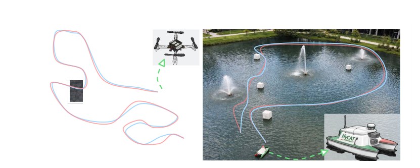
Fig. 6: Qualitative results. Full-compute trajectories (GC-Diffuser and B-COD teacher) are shown in red; Muninn-accelerated trajectories are shown in blue.
图 6:定性结果。全程计算轨迹(GC-Diffuser 和 B-COD 教师)用红色表示;经 Muninn 加速的轨迹用蓝色表示。
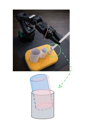
Fig. 7: Angle of attacks (hard peg insertion) Red: Diffusion Policy; blue: Muninn.
图 7:攻角(困难插销)。红色:Diffusion Policy;蓝色:Muninn。
TABLE IV: We compare the Full (teacher) models against the baselines and Muninn on the waypoint navigation and manipulation (averaged over three tasks) tasks. (Average of 150 hardware runs).
| Pl. | Method | Lat. (ms) | Succ. (%) | Coll. (%) |
|---|---|---|---|---|
| BCOD [48] | 12 | 94.0 | 2.4 | |
| BCOD [48] | 60 | 97.0 | 1.6 | |
| BCOD + Muninn | 24 | 96.8 | 1.7 | |
| ASV | GC-Diff. [21] | 70 | 95.5 | 2.2 |
| GC-Diff. + Muninn | 28 | 95.3 | 2.3 | |
| UAV | GC-Diff. [21] | 75 | 93.0 | 3.0 |
| GC-Diff. + Muninn | 30 | 92.8 | 3.1 | |
| SO-100 | Diff. policy [9] | 40 | 82.0 | 6.0 |
| DP + Muninn | 24 | 81.5 | 6.2 |
表 IV:我们在航点导航和操作(对三项任务取平均)任务上,把 Full(教师)模型与基线及 Muninn 比较。(150 次硬件运行的平均)。
| 平台 | 方法 | 延迟(毫秒) | 成功率(%) | 碰撞(%) |
|---|---|---|---|---|
| BCOD [48] | 12 | 94.0 | 2.4 | |
| BCOD [48] | 60 | 97.0 | 1.6 | |
| BCOD + Muninn | 24 | 96.8 | 1.7 | |
| ASV | GC-Diff. [21] | 70 | 95.5 | 2.2 |
| GC-Diff. + Muninn | 28 | 95.3 | 2.3 | |
| UAV | GC-Diff. [21] | 75 | 93.0 | 3.0 |
| GC-Diff. + Muninn | 30 | 92.8 | 3.1 | |
| SO-100 | Diff. policy [9] | 40 | 82.0 | 6.0 |
| DP + Muninn | 24 | 81.5 | 6.2 |
C. Key findings, analysis, and ablations
C. 主要发现、分析与消融
As can be seen from the results in sections V-A and V-B, Muninn consistently reduces denoiser evaluations and wall-clock latency across all evaluated policies while preserving task performance. We now report key findings (KF) and summarize ablations of Muninn’s internal design choices, with further breakdowns deferred to Appendix D.
从第 V-A 节和第 V-B 节的结果可以看出,Muninn 在所有评估过的策略上都一致地减少去噪器评估次数和墙钟延迟,同时保持任务表现。我们接下来报告关键发现(KF),并概括对 Muninn 内部设计选择的消融,更细的分解放到附录 D。
(KF#1) Muninn dominates inference-time acceleration baselines on the task–latency–risk Pareto frontier. A common path to real-time diffusion planning is training-free inference-time acceleration, i.e., reducing denoiser work without retraining. Most such methods are compute-centric: they skip calls without modeling how errors propagate through the sampler or impact the final trajectory. We compare Muninn against three such baselines (Fig. 8, Table V): (i) FewSteps[47]: run the same pretrained denoiser with a reduced diffusion horizon . (ii) FixedSkip: evaluate the denoiser every steps and reuse the last predicted noise for skipped steps. (iii) ProbeThresh: reuse if the probe-change falls below a tuned threshold .
(KF#1)Muninn 在任务–延迟–风险帕累托前沿上主导推理时加速基线。通向实时扩散规划的一条常见路径,是无需训练的推理时加速,也就是在不重新训练的情况下减少去噪器工作量。这类方法大多以计算为中心:它们跳过调用,却不建模误差如何通过采样器传播,或如何影响最终轨迹。我们把 Muninn 与三条这样的基线比较(图 8,表 V):(i) FewSteps[47]:用缩短的扩散时域 运行同一个预训练去噪器。(ii) FixedSkip: 每隔 步评估一次去噪器,对被跳过的步骤复用最近一次预测的噪声。(iii) ProbeThresh: 若探针变化 落到调好的阈值 以下,则复用。
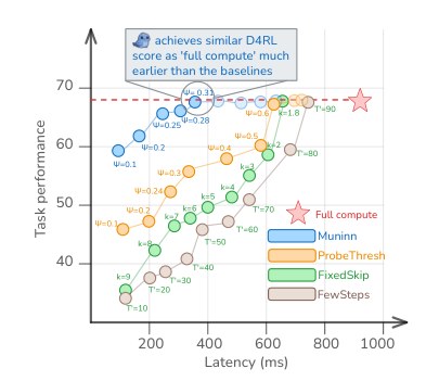
Fig. 8: We plot the D4RL score vs. wall-clock latency for D4RL AntMaze. Muninn achieves the same task success rate as Full model quicker than the baselines.
图 8:我们画出 D4RL AntMaze 上 D4RL 分数相对墙钟延迟的曲线。Muninn 达到与 Full 模型相同的任务成功率,比基线快 。
TABLE V: We compare the Full (unmodified -step sampler) model against the baselines and Muninn on the D4RL AntMaze task. The results above correspond to allowing Full to run for 957 ms, at which point it achieves the maximum possible D4RL score. The baselines and Muninn are capped at 250 ms (approximately 1/4th of the runtime).
| Method | Task | ||
|---|---|---|---|
| Full | 68.7 | 0.00 | 0.00 |
| FewSteps | 56.1 | 0.12 | 0.17 |
| FixedSkip | 42.5 | 0.10 | 0.14 |
| ProbeThresh | 48.0 | 0.09 | 0.10 |
| + Full (Muninn) | 67.6 | 0.07 | 0.04 |
表 V:我们在 D4RL AntMaze 任务上,把 Full(未经修改的 步采样器)模型与基线及 Muninn 比较。上表结果对应允许 Full 运行 957 毫秒,此时它达到可能的最高 D4RL 分数。基线和 Muninn 被限制在 250 毫秒(大约是运行时间的四分之一)。
| 方法 | 任务 | ||
|---|---|---|---|
| Full | 68.7 | 0.00 | 0.00 |
| FewSteps | 56.1 | 0.12 | 0.17 |
| FixedSkip | 42.5 | 0.10 | 0.14 |
| ProbeThresh | 48.0 | 0.09 | 0.10 |
| + Full (Muninn) | 67.6 | 0.07 | 0.04 |
Considering the offline RL domain (averaged across benchmarks in Table I), we find that Muninn yields a strictly better operating curve: at the same latency it preserves task success more reliably, and at the same it achieves lower latency. This happens because FewSteps and FixedSkip implicitly allocate approximation error uniformly in diffusion time, even though the sampler’s sensitivity profile is highly non-uniform. ProbeThresh adapts to probe dynamics, but without calibrated error envelopes it violates risk in hard contexts or becomes overly conservative when tuned for safety. The baselines inherently produce small latent errors that become large deviations after downstream sampler mixing. Muninn is the only inference-time method in this set that (a) estimates reuse error with distribution-free coverage and (b) accounts for step-dependent error amplification through .
在离线强化学习领域(对表 I 中各基准取平均),我们发现 Muninn 给出一条严格更优的工作曲线:在相同延迟下,它更可靠地保持任务成功;在相同的 下,它达到更低延迟。原因在于,FewSteps 和 FixedSkip 隐含地把近似误差在扩散时间上均匀分配,尽管采样器的敏感性剖面 高度不均匀。ProbeThresh 会适应探针动态,但没有经过校准的误差包络,它会在困难情境中违反风险,或在为安全而调参时过于保守。这些基线本质上会产生很小的潜在误差,它们在下游采样器混合之后变成大偏差。在这一组里,Muninn 是唯一既(a)以与分布无关的覆盖来估计复用误差,又(b)通过 计入步依赖误差放大的推理时方法。
(KF #2) Muninn closes much of the gap to training-time accelerations without retraining. A second path to real-time diffusion planning is training-time acceleration. These methods can achieve very low latency, but require additional training compute, careful hyperparameter sweeps, and often task- or architecture-specific redesign. We compare Muninn (Fig. 9, Table VI) against: (i) Distill-1step/Distill-Kstep[63, 66]: one/few-step distilled planners, (ii) SmallNet:[66] a smaller denoiser trained from scratch or fine-tuned (fewer layers / width), (iii) LearnedExit[71]: a trained controller that predicts early stopping.
(KF #2)Muninn 在不重新训练的情况下,弥合了与训练时加速之间的大部分差距。通向实时扩散规划的第二条路径是训练时加速。这些方法可以把延迟压得很低,但需要额外的训练计算、细致的超参数扫描,并且常常要针对任务或架构重新设计。我们把 Muninn(图 9,表 VI)与以下方法比较:(i) Distill-1step / Distill-Kstep[63, 66]:一步 / 少步蒸馏规划器;(ii) SmallNet:[66] 从零训练或微调得到的更小去噪器(更少层数 / 宽度);(iii) LearnedExit[71]:一个训练好的控制器,用于预测提前停止。
TABLE VI: Columns report whether each method requires extra training compute, additional data (beyond the original training set), or architectural changes for the DP3 Pour benchmark. We include Distill+Muninn to show composability. Legend: = none, = yes, = often, = moderate, = high.
| Method | Extra train. | Extra data | Arch. change |
|---|---|---|---|
| Full multi-step (teacher) | |||
| Distill-1step | |||
| Distill-Kstep (K=4) | |||
| SmallNet (0.6 width) | |||
| LearnedExit | |||
| Teacher + Muninn | |||
| Distill-Kstep + Muninn |
表 VI:各列报告每一种方法在 DP3 Pour 基准上是否需要额外训练计算、额外数据(超出原始训练集),或架构改动。我们纳入 Distill+Muninn 以展示可组合性。图例: = 无, = 是, = 经常, = 中等, = 高。
| 方法 | 额外训练 | 额外数据 | 架构改动 |
|---|---|---|---|
| Full multi-step (teacher) | |||
| Distill-1step | |||
| Distill-Kstep (K=4) | |||
| SmallNet (0.6 width) | |||
| LearnedExit | |||
| Teacher + Muninn | |||
| Distill-Kstep + Muninn |
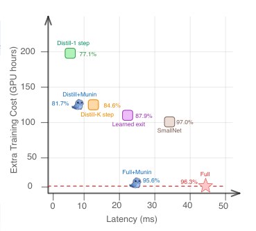
Fig. 9: Scatter plot summarizing the practical acceleration spectrum on the DP3 Pour diffusion policy. We also report the average success percentage of these models during inference. GPU-hours are normalized to A10 24GB-hours equivalent. More details about the training procedure is available in the Appendix.
图 9:概括 DP3 Pour 扩散策略上实际加速谱系的散点图。我们也报告这些模型在推理时的平均成功百分比。GPU 小时数被归一化到等效的 A10 24GB 小时。训练流程的更多细节见附录。
We find that Muninn provides a deployment-friendly point on the spectrum: it recovers a large fraction of the achievable latency reduction immediately, while preserving the behavior of the original planner. Moreover, Muninn is composable: applying Muninn on top of a distilled or compact model yields additional speedups, because Muninn targets redundant per-step computation that remains even in fewer-step samplers.
我们发现 Muninn 在这一谱系上提供了一个便于部署的点:它立刻收回可实现延迟降幅中的很大一部分,同时保持原规划器的行为。此外,Muninn 是可组合的:在蒸馏或紧凑模型之上再施加 Muninn,还能得到额外加速,因为即便在更少步的采样器中,Muninn 针对的逐步冗余计算仍然存在。
(KF#3) Muninn induces difficulty-adaptive compute.
(KF#3)Muninn 会诱导随难度自适应的计算。
TABLE VII: Left: Episode fraction and Muninn success binned by #evaluations: low-eval bins are easier (higher success), high-eval bins are harder (lower success). Right: Compute and success vs. minimum-clearance difficulty: Muninn uses more evals. in harder and fewer in easier regions.
| Eval bin | Fraction eps. | Success | Min. clearance | Avg. evals | Success |
|---|---|---|---|---|---|
| 10–12 | 0.20 | 0.99 | 0.1 | 22 | 0.84 |
| 13–15 | 0.30 | 0.97 | 0.3 | 20 | 0.90 |
| 16–18 | 0.25 | 0.94 | 0.5 | 18 | 0.94 |
| 19–21 | 0.15 | 0.90 | 0.7 | 15 | 0.97 |
| 22–25 | 0.10 | 0.87 | 0.9 | 12 | 0.99 |
表 VII:左: 按评估次数分箱的回合比例和 Muninn 成功率:低评估箱更容易(成功率更高),高评估箱更难(成功率更低)。右: 计算量和成功率相对最小间隙难度:Muninn 在更难区域用更多评估,在更容易区域用更少评估。
| 评估箱 | 回合比例 | 成功率 | 最小间隙 | 平均评估次数 | 成功率 |
|---|---|---|---|---|---|
| 10–12 | 0.20 | 0.99 | 0.1 | 22 | 0.84 |
| 13–15 | 0.30 | 0.97 | 0.3 | 20 | 0.90 |
| 16–18 | 0.25 | 0.94 | 0.5 | 18 | 0.94 |
| 19–21 | 0.15 | 0.90 | 0.7 | 15 | 0.97 |
| 22–25 | 0.10 | 0.87 | 0.9 | 12 | 0.99 |
A hidden cost of fixed accelerations is that they spend the same compute on easy and hard situations. In robotics, difficulty varies across time (e.g., open-space navigation vs. tight corridors).
固定加速的一个隐性代价,是它们在容易和困难的情境上花掉同样的计算。在机器人学中,难度会随时间变化(例如开阔空间导航与狭窄走廊)。
Muninn’s decision rule is inherently state- and context-adaptive. Taking the example of cluttered 7-DoF arm planning (averaged across EDMP and MPD) (Table VII), we analyze the distribution of denoiser evaluations per episode and correlate it with environment difficulty proxies. The left panel in Table VII should be read as a distribution over Muninn’s actual compute usage: episodes that require only 10–12 denoiser evaluations are typically easier and succeed more often, while episodes that consume 22–25 evaluations are harder and have lower success. The right panel Table VII makes this difficulty axis explicit using minimum clearance: as clearance decreases from open-space to tight-clutter settings, Muninn automatically recomputes more often instead of applying a fixed skip pattern. We find that Muninn naturally allocates more compute to high-risk or high-uncertainty regimes, and aggressively reuses outputs when the diffusion trajectory stabilizes.
Muninn 的决策规则本质上对状态和上下文自适应。以杂乱环境中的 7 自由度手臂规划为例(对 EDMP 和 MPD 取平均)(表 VII),我们分析每个回合的去噪器评估次数分布,并把它与环境难度代理关联起来。表 VII 的左栏应读作 Muninn 实际计算用量的分布:只需 10–12 次去噪器评估的回合通常更容易、成功也更频繁,而消耗 22–25 次评估的回合更难、成功率更低。表 VII 的右栏用最小间隙把这一难度轴说清楚:当间隙从开阔空间降到紧密杂乱设定时,Muninn 会自动更频繁地重算,而不是套用固定的跳步模式。我们发现,Muninn 会自然地把更多计算分配给高风险或高不确定性的情形,并在扩散轨迹稳定时积极复用输出。
(KF#4) Muninn’s budget accounting produces a usable runtime certificate that correlates with downstream safety. Most acceleration methods are opaque: they reduce compute, but provide no introspection about when approximations become dangerous. Muninn is different because its internal quantity is an explicit, online-tracked upper bound proxy (Fig. 10) for how far the cached trajectory might drift from full compute. This yields two practical benefits: (i) Post-hoc explainability: we can attribute most deviation risk to specific timesteps and contexts where is large and the probe indicates instability. (ii) Runtime escalation: in a closed-loop controller, we can treat low remaining budget or large as a trigger to (a) temporarily run full compute, (b) reduce the action magnitude, (c) switch to a conservative safety controller, or (d) request more samples. We present an extended study of the runtime escalations in the Appendix D.
(KF#4)Muninn 的预算核算产生一份可用的运行时证书,它与下游安全相关。多数加速方法是不透明的:它们减少计算,却不提供近似何时变得危险的内省。Muninn 不同,因为它的内部量 是一个显式、在线跟踪的上界代理(图 10),用来描述缓存轨迹可能偏离全程计算有多远。这带来两点实际好处:(i) 事后可解释性: 我们可以把大部分偏差风险归因到 较大、且探针表明不稳定的特定时间步和情境。(ii) 运行时升级: 在闭环控制器中,可以把剩余预算 偏低或 偏大,当作触发去(a)暂时跑全程计算,(b)减小动作幅度,(c)切换到保守的安全控制器,或(d)请求更多样本。我们在附录 D 中给出运行时升级的扩展研究。
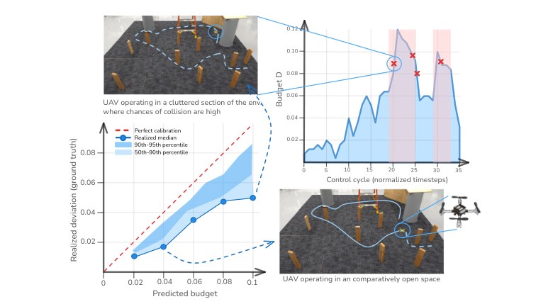
Fig. 10: Left: Reliability plot: predicted vs. realized deviation ; Muninn is monotone and conservative (below the diagonal). Right: GC-Diffuser+Muninn on 3D UAV navigation: over control cycles, with spikes aligning to near-collision/contact events (red); callouts show the UAV pose at those instants.
图 10:左:可靠性图:预测的 相对实现偏差 ;Muninn 是单调且保守的(在对角线下方)。右:GC-Diffuser+Muninn 在三维无人机导航上: 随控制周期变化,尖峰与近碰撞 / 接触事件对齐(红色);标注给出那些瞬间的无人机位姿。
Ablations. We ablate Munin’s key design choices and report a detailed summary in Appendix D. Overall, (i) increasing the trajectory deviation budget yields a smooth speed–fidelity knob (more reuse equals higher speedup with minor performance loss); (ii) split-conformal calibration is necessary to reliably achieve a target violation probability , while heuristic rules miscalibrate; (iii) sensitivity-aware budgeting via sampler coefficients improves the speed–safety trade-off by allocating recomputation to high-impact timesteps; (iv) shallow stem probes provide the best net speedups (good predictiveness at low overhead); (v) forbidding reuse in a small prefix/suffix further reduces collisions/violations with modest speed loss; and (vi) calibration is sample-efficient, with risk and speed stabilizing after a modest number of rollouts.
消融。我们对 Muninn 的关键设计选择做了消融,并在附录 D 中报告详细概括。总体而言,(i)增大轨迹偏差预算 会给出一条平滑的速度–保真旋钮(更多复用等于更高加速,表现只轻微下降);(ii)要可靠地达到目标违反概率 ,分裂共形校准是必要的,启发式规则会校准不准;(iii)借助采样器系数 做敏感性感知的预算分配,能通过把重算分配到高影响时间步来改善速度–安全权衡;(iv)浅层茎干探针给出最好的净加速(预测性好、开销低);(v)在一小段前缀 / 后缀禁止复用,能以不大的速度损失进一步减少碰撞 / 违反;以及(vi)校准在样本上是高效的,风险和速度在适量滚动之后就会稳定。
VI. Conclusion
VI. 结论
This work introduces Muninn, a training-free caching wrapper that accelerates trajectory diffusion models without modifying model weights or the sampler. Muninn leverages two signals that are present in trajectory diffusion planners: (i) a cheap probe of how the model’s internal representation evolves across denoising steps, and (ii) analytic sampler sensitivity coefficients that quantify how denoiser perturbations propagate into the final trajectory. By calibrating probe dynamics against potential reuse error, Muninn produces step-wise, distribution-free error envelopes that can be converted into a trajectory-level deviation budget. At run time, Muninn spends this budget to decide when cached denoiser outputs can be safely reused. Across simulated benchmarks and hardware experiments, Muninn substantially reduces denoiser evaluations and wall-clock latency while preserving task performance and safety metrics. A promising direction for future work is to replace the current fixed user-specified deviation budget with a context-aware budget that automatically tightens in cluttered or contact-rich regimes and relaxes in open-space or low-risk regimes.
本文介绍 Muninn,这是一个无需训练的缓存封装,用于加速轨迹扩散模型,而不修改模型权重或采样器。Muninn 利用轨迹扩散规划器中已有的两种信号:(i)对模型内部表示如何随去噪步骤演化的廉价探针,以及(ii)解析的采样器敏感性系数,用来量化去噪器扰动如何传播到最终轨迹。通过把探针动态对着潜在复用误差做校准,Muninn 产生逐步的、与分布无关的误差包络,并可以把它们换成轨迹级偏差预算。运行时,Muninn 花掉这笔预算,来决定何时可以安全地复用缓存的去噪器输出。在仿真基准和硬件实验中,Muninn 大幅减少去噪器评估次数和墙钟延迟,同时保持任务表现和安全指标。一个有前景的未来方向,是用上下文感知的预算替换当前由用户固定指定的偏差预算,在杂乱或富接触情形中自动收紧,在开阔空间或低风险情形中放宽。
Acknowledgements
致谢
This work was supported in part by NSF grants 2118329, IIS-2024733 and IIS-2331908, the Office of Naval Research grants N00014-23-1-2505, N00014-25-1-2519, N00014-23-1-2789, the U.S. Department of Defense grant 78170-RT-REP, and by the Army Research Laboratories under contract W911NF1920243. This is contribution #2135 from the Institute of Environment at Florida International University.
本工作部分得到 NSF 基金 2118329、IIS-2024733 和 IIS-2331908,海军研究办公室基金 N00014-23-1-2505、N00014-25-1-2519、N00014-23-1-2789,美国国防部基金 78170-RT-REP,以及陆军研究实验室合同 W911NF1920243 的支持。这是佛罗里达国际大学环境研究所的第 2135 号贡献。
References
参考文献
[1] Shubham Agarwal, Subrata Mitra, Sarthak Chakraborty, Srikrishna Karanam, Koyel Mukherjee, and Shiv Kumar Saini. Approximate caching for efficiently serving Text-to-Image diffusion models. In USENIX Symposium on Networked Systems Design and Implementation , pages 1173–1189, 2024.
[2] Anurag Ajay, Yilun Du, Abhi Gupta, Joshua B. Tenenbaum, Tommi Jaakkola, and Pulkit Agrawal. Is conditional generative modeling all you need for decision-making? arXiv preprint arXiv:2211.15657 , 2022.
[3] Kevin Black, Michael Janner, Yilun Du, Ilya Kostrikov, and Sergey Levine. Training diffusion models with reinforcement learning. arXiv preprint arXiv:2305.13301 , 2023.
[4] Daniel Bolya and Judy Hoffman. Token merging for fast stable diffusion. In IEEE/CVF Conference on Computer Vision and Pattern Recognition , pages 4599–4603, 2023.
[5] Jiazi Bu, Pengyang Ling, Yujie Zhou, Yibin Wang, Yuhang Zang, Tong Wu, Dahua Lin, and Jiaqi Wang. Dicache: Let diffusion model determine its own cache. arXiv preprint arXiv:2508.17356 , 2025.
[6] Joao Carvalho, An T Le, Mark Baierl, Dorothea Koert, and Jan Peters. Motion planning diffusion: Learning and planning of robot motions with diffusion models. In IEEE/RSJ International Conference on Intelligent Robots and Systems , pages 1916–1923, 2023.
[7] Guanjie Chen, Xinyu Zhao, Yucheng Zhou, Tianlong Chen, and Cheng Yu. Accelerating vision diffusion transformers with skip branches. arXiv preprint arXiv:2411.17616 , 2024a.
[8] Yuzhu Chen, Fengxiang He, Shi Fu, Xinmei Tian, and Dacheng Tao. Adaptive time-stepping schedules for diffusion models. In Conference on Uncertainty in Artificial Intelligence , 2024b.
[9] Cheng Chi, Zhenjia Xu, Siyuan Feng, Eric Cousineau, Yilun Du, Benjamin Burchfiel, Russ Tedrake, and Shuran Song. Diffusion policy: Visuomotor policy learning via action diffusion. The International Journal of Robotics Research , 44(10-11):1684–1704, 2025.
[10] Felipe Codevilla, Matthias Müller, Antonio López, Vladlen Koltun, and Alexey Dosovitskiy. End-to-end driving via conditional imitation learning. In IEEE International Conference on Robotics and Automation , pages 4693–4700, 2018.
[11] Justin Fu, Aviral Kumar, Ofir Nachum, G. Tucker, and Sergey Levine. D4rl: Datasets for deep data-driven reinforcement learning. arXiv preprint arXiv:2004.07219 , 2020.
[12] Alex Graves. Adaptive computation time for recurrent neural networks. arXiv preprint arXiv:1603.08983 , 2016.
[13] Agrim Gupta, Justin Johnson, Li Fei-Fei, Silvio Savarese, and Alexandre Alahi. Social GAN: Socially acceptable trajectories with generative adversarial networks. In IEEE/CVF Conference on Computer Vision and Pattern Recognition , pages 2255–2264, 2018.
[14] Jonathan Ho and Tim Salimans. Classifier-free diffusion guidance. arXiv preprint arXiv:2207.12598 , 2022.
[15] Jonathan Ho, Ajay Jain, and Pieter Abbeel. Denoising diffusion probabilistic models. In Neural Information Processing Systems , volume 33, pages 6840–6851, 2020.
[16] Jonathan Ho, Chitwan Saharia, William Chan, David J. Fleet, Mohammad Norouzi, and Tim Salimans. Cascaded diffusion models for high fidelity image generation. Journal of Machine Learning Research , 23(47):1–33, 2022.
[17] Renming Huang, Yunqiang Pei, Guoqing Wang, Yangming Zhang, Yang Yang, Peng Wang, and Hengtao Shen. Diffusion models as optimizers for efficient planning in offline RL. In European Conference on Computer Vision , pages 1–17, 2024.
[18] Siyuan Huang, Zan Wang, Puhao Li, Baoxiong Jia, Tengyu Liu, Yixin Zhu, Wei Liang, and Song-Chun Zhu. Diffusion-based generation, optimization, and planning in 3D scenes. In IEEE/CVF Conference on Computer Vision and Pattern Recognition , pages 16750–16761, 2023.
[19] Boris Ivanovic and Marco Pavone. The Trajectron: Probabilistic multi-agent trajectory modeling with dynamic spatiotemporal graphs. In IEEE/CVF International Conference on Computer Vision , pages 2375–2384, 2019.
[20] Stephen James, Zicong Ma, David Rovick Arrojo, and Andrew J. Davison. Rlbench: The robot learning benchmark & learning environment. IEEE Robotics and Automation Letters , 5:3019–3026, 2019.
[21] Michael Janner, Yilun Du, Joshua B Tenenbaum, and Sergey Levine. Planning with diffusion for flexible behavior synthesis. arXiv preprint arXiv:2205.09991 , 2022.
[22] Hyeonseong Jeon, Cheolhong Min, and Jaesik Park. Tree-guided diffusion planner. arXiv preprint arXiv:2508.21800 , 2025.
[23] Mrinal Kalakrishnan, Sachin Chitta, Evangelos Theodorou, Peter Pastor, and Stefan Schaal. Stomp: Stochastic trajectory optimization for motion planning. In IEEE International Conference on Robotics and Automation , pages 4569–4574, 2011.
[24] Tero Karras, Miika Aittala, Timo Aila, and Samuli Laine. Elucidating the design space of diffusion-based generative models. In Neural Information Processing Systems , volume 35, pages 26565–26577, 2022.
[25] Diederik P Kingma and Max Welling. Auto-encoding variational Bayes. arXiv preprint arXiv:1312.6114 , 2013.
[26] Namhoon Lee, Wongun Choi, Paul Vernaza, Christopher B Choy, Philip HS Torr, and Manmohan Chandraker. Desire: Distant future prediction in dynamic scenes with interacting agents. In IEEE/CVF Conference on Computer Vision and Pattern Recognition , pages 336–345, 2017.
[27] Lijiang Li, Huixia Li, Xiawu Zheng, Jie Wu, Xuefeng Xiao, Rui Wang, Min Zheng, Xin Pan, Fei Chao, and Rongrong Ji. Autodiffusion: Training-free optimization of time steps and architectures for automated diffusion model acceleration. In IEEE/CVF International Conference on Computer Vision , pages 7105–7114, 2023.
[28] Weiwei Li and Emanuel Todorov. Iterative linear quadratic regulator design for nonlinear biological movement systems. In International Conference on Informatics in Control, Automation and Robotics , pages 222–229, 2004.
[29] Zhixuan Liang, Yao Mu, Mingyu Ding, Fei Ni, Masayoshi Tomizuka, and Ping Luo. AdaptDiffuser: Diffusion models as adaptive self-evolving planners. arXiv preprint arXiv:2302.01877 , 2023.
[30] Weijie Liu, Peng Zhou, Zhiruo Wang, Zhe Zhao, Haotang Deng, and Qi Ju. FastBERT: A self-distilling BERT with adaptive inference time. In Annual Meeting of the Association for Computational Linguistics , pages 6035–6044, 2020.
[31] Cheng Lu, Yuhao Zhou, Fan Bao, Jianfei Chen, Chongxuan Li, and Jun Zhu. DPM-Solver: A fast ODE solver for diffusion probabilistic model sampling in around 10 steps. In Neural Information Processing Systems , volume 35, pages 5775–5787, 2022.
[32] Haofei Lu, Dongqi Han, Yifei Shen, and Dongsheng Li. What makes a good diffusion planner for decision making? arXiv preprint arXiv:2503.00535 , 2025.
[33] Kairong Luo, Caiwei Xiao, Zhiao Huang, Zhan Ling, Yunhao Fang, and Hao Su. Dreamfuser: Value-guided diffusion policy for offline reinforcement learning.
[34] Yunhao Luo, Chen Sun, Joshua B. Tenenbaum, and Yilun Du. Potential-based diffusion motion planning. arXiv preprint arXiv:2407.06169 , 2024.
[35] Yunhao Luo, Utkarsh A. Mishra, Yilun Du, and Danfei Xu. Generative trajectory stitching through diffusion composition. arXiv preprint arXiv:2503.05153 , 2025.
[36] Zhengyao Lv, Chenyang Si, Junhao Song, Zhenyu Yang, Yu Qiao, Ziwei Liu, and Kwan-Yee K Wong. Fastercache: Training-free video diffusion model acceleration with high quality. arXiv preprint arXiv:2410.19355 , 2024.
[37] Zhaoyang Lyu, Xudong Xu, Ceyuan Yang, Dahua Lin, and Bo Dai. Accelerating diffusion models via early stop of the diffusion process. arXiv preprint arXiv:2205.12524 , 2022.
[38] Xinyin Ma, Gongfan Fang, Michael Bi Mi, and Xinchao Wang. Learning-to-cache: Accelerating diffusion transformer via layer caching. In Neural Information Processing Systems , volume 37, pages 133282–133304, 2024a.
[39] Xinyin Ma, Gongfan Fang, and Xinchao Wang. Deepcache: Accelerating diffusion models for free. In IEEE/CVF Conference on Computer Vision and Pattern Recognition , pages 15762–15772, 2024b.
[40] Xinyin Ma, Runpeng Yu, Gongfan Fang, and Xinchao Wang. DKV-Cache: The cache for diffusion language models. arXiv preprint arXiv:2505.15781 , 2025.
[41] David Q Mayne, James B Rawlings, Christopher V Rao, and Pierre OM Scokaert. Constrained model predictive control: Stability and optimality. Automatica , 36(6):789–814, 2000.
[42] Chenlin Meng, Robin Rombach, Ruiqi Gao, Diederik Kingma, Stefano Ermon, Jonathan Ho, and Tim Salimans. On distillation of guided diffusion models. In IEEE/CVF Conference on Computer Vision and Pattern Recognition , pages 14297–14306, 2023.
[43] Taehong Moon, Moonseok Choi, EungGu Yun, Jongmin Yoon, Gayoung Lee, and Juho Lee. Early exiting for accelerated inference in diffusion models. In ICML Workshop on Structured Probabilistic Inference & Generative Modeling , 2023.
[44] Taehong Moon, Moonseok Choi, EungGu Yun, Jongmin Yoon, Gayoung Lee, Jaewoong Cho, and Juho Lee. A simple early exiting framework for accelerated sampling in diffusion models. arXiv preprint arXiv:2408.05927 , 2024.
[45] Alexander Quinn Nichol and Prafulla Dhariwal. Improved denoising diffusion probabilistic models. In International Conference on Machine Learning , pages 8162–8171, 2021.
[46] Chaoyi Pan, Zeji Yi, Guanya Shi, and Guannan Qu. Model-based diffusion for trajectory optimization. In Neural Information Processing Systems , volume 37, pages 57914–57943, 2024.
[47] Aaditya Prasad, Kevin Lin, Jimmy Wu, Linqi Zhou, and Jeannette Bohg. Consistency policy: Accelerated visuomotor policies via consistency distillation. arXiv preprint arXiv:2405.07503 , 2024.
[48] Gokul Puthumanaillam, Aditya Penumarti, Manav Vora, Paulo Padrao, Jose Fuentes, Leonardo Bobadilla, Jane Shin, and Melkior Ornik. Belief-conditioned one-step diffusion: Real-time trajectory planning with just-enough sensing. In Conference on Robot Learning , pages 68–92, 2025.
[49] Robin Rombach, Andreas Blattmann, Dominik Lorenz, Patrick Esser, and Björn Ommer. High-resolution image synthesis with latent diffusion models. In IEEE/CVF Conference on Computer Vision and Pattern Recognition , pages 10684–10695, 2022.
[50] Stéphane Ross, Geoffrey Gordon, and Drew Bagnell. A reduction of imitation learning and structured prediction to no-regret online learning. In International Conference on Artificial Intelligence and Statistics , pages 627–635, 2011.
[51] Kallol Saha, Vishal Mandadi, Jayaram Reddy, Ajit Srikanth, Aditya Agarwal, Bipasha Sen, Arun Singh, and Madhava Krishna. EDMP: Ensemble-of-costs-guided diffusion for motion planning. In IEEE International Conference on Robotics and Automation , pages 10351–10358, 2024.
[52] Tim Salimans and Jonathan Ho. Progressive distillation for fast sampling of diffusion models. arXiv preprint arXiv:2202.00512 , 2022.
[53] Christoph Schöller and Alois Knoll. Flomo: Tractable motion prediction with normalizing flows. In IEEE/RSJ International Conference on Intelligent Robots and Systems , pages 7977–7984, 2021.
[54] John Schulman, Jonathan Ho, Alex X Lee, Ibrahim Awwal, Henry Bradlow, and Pieter Abbeel. Finding locally optimal, collision-free trajectories with sequential convex optimization. In Robotics: Science and Systems , 2013.
[55] Mingyo Seo, Yoonyoung Cho, Yoonchang Sung, Peter Stone, Yuke Zhu, and Beomjoon Kim. Presto: Fast motion planning using diffusion models based on key-configuration environment representation. In IEEE International Conference on Robotics and Automation , pages 10861–10867, 2025.
[56] Yorai Shaoul, Itamar Mishani, Shivam Vats, Jiaoyang Li, and Maxim Likhachev. Multi-robot motion planning with diffusion models. arXiv preprint arXiv:2410.03072 , 2024.
[57] Jiaming Song, Chenlin Meng, and Stefano Ermon. Denoising diffusion implicit models. arXiv preprint arXiv:2010.02502 , 2020a.
[58] Yang Song, Jascha Sohl-Dickstein, Diederik P Kingma, Abhishek Kumar, Stefano Ermon, and Ben Poole. Score-based generative modeling through stochastic differential equations. arXiv preprint arXiv:2011.13456 , 2020b.
[59] Yang Song, Prafulla Dhariwal, Mark Chen, and Ilya Sutskever. Consistency models. 2023.
[60] Surat Teerapittayanon, Bradley McDanel, and Hsiang-Tsung Kung. Branchynet: Fast inference via early exiting from deep neural networks. In International Conference on Pattern Recognition , pages 2464–2469, 2016.
[61] Xin Wang, Fisher Yu, Zi-Yi Dou, Trevor Darrell, and Joseph E Gonzalez. SkipNet: Learning dynamic routing in convolutional networks. In European Conference on Computer Vision , pages 409–424, 2018.
[62] Zhendong Wang, Jonathan J. Hunt, and Mingyuan Zhou. Diffusion policies as an expressive policy class for offline reinforcement learning. arXiv preprint arXiv:2208.06193 , 2022.
[63] Zhendong Wang, Zhaoshuo Li, Ajay Mandlekar, Zhenjia Xu, Jiaojiao Fan, Yashraj S. Narang, Linxi Fan, Yuke Zhu, Yogesh Balaji, Mingyuan Zhou, Ming-Yu Liu, and Yuan Zeng. One-step diffusion policy: Fast visuomotor policies via diffusion distillation. arXiv preprint arXiv:2410.21257 , 2024.
[64] Grady Williams, Andrew Aldrich, and Evangelos Theodorou. Model predictive path integral control: From theory to parallel computation. Journal of Guidance, Control, and Dynamics , 40(2):344–357, 2017.
[65] Rosa Wolf, Yitian Shi, Sheng Liu, and Rania Rayyes. Diffusion models for robotic manipulation: A survey. arXiv preprint arXiv:2504.08438 , 2025.
[66] Yiming Wu, Huan Wang, Zhenghao Chen, Jianxin Pang, and Dong Xu. On-device diffusion transformer policy for efficient robot manipulation. arXiv preprint arXiv:2508.00697 , 2025.
[67] Zhou Xian, Nikolaos Gkanatsios, Theophile Gervet, Tsung-Wei Ke, and Katerina Fragkiadaki. Chaineddiffuser: Unifying trajectory diffusion and keypose prediction for robotic manipulation. In Conference on Robot Learning , 2023.
[68] Sirui Xie, Zhisheng Xiao, Diederik Kingma, Tingbo Hou, Ying Nian Wu, Kevin P Murphy, Tim Salimans, Ben Poole, and Ruiqi Gao. EM distillation for one-step diffusion models. In Neural Information Processing Systems , volume 37, pages 45073–45104, 2024.
[69] Tianwei Yin, Michaël Gharbi, Richard Zhang, Eli Shechtman, Fredo Durand, William T Freeman, and Taesung Park. One-step diffusion with distribution matching distillation. arXiv preprint arXiv:2311.18828 , 2023.
[70] Tianhe Yu, Deirdre Quillen, Zhanpeng He, Ryan C. Julian, Karol Hausman, Chelsea Finn, and Sergey Levine. Meta-world: A benchmark and evaluation for multi-task and meta reinforcement learning. In Conference on Robot Learning , 2019.
[71] Yanjie Ze, Gu Zhang, Kangning Zhang, Chenyuan Hu, Muhan Wang, and Huazhe Xu. 3d diffusion policy: Generalizable visuomotor policy learning via simple 3d representations. In Robotics: Science and Systems (RSS) , 2024.
[72] Zheng Zhan, Yushu Wu, Yifan Gong, Zichong Meng, Zhenglun Kong, Changdi Yang, Geng Yuan, Pu Zhao, Wei Niu, and Yanzhi Wang. Fast and memory-efficient video diffusion using streamlined inference. In Neural Information Processing Systems , volume 37, pages 13660–13684, 2024.
[73] Hui Zhang, Zuxuan Wu, Zhen Xing, Jie Shao, and Yu-Gang Jiang. AdaDiff: Adaptive step selection for fast diffusion models. In AAAI Conference on Artificial Intelligence , volume 39, pages 9914–9922, 2025.
[74] Zhengbang Zhu, Hanye Zhao, Haoran He, Yichao Zhong, Shenyu Zhang, Yong Yu, and Weinan Zhang. Diffusion models for reinforcement learning: A survey. arXiv preprint arXiv:2311.01223 , 2023.
[75] Zhengbang Zhu, Minghuan Liu, Liyuan Mao, Bingyi Kang, Minkai Xu, Yong Yu, Stefano Ermon, and Weinan Zhang. MaDiff: Offline multi-agent learning with diffusion models. In Neural Information Processing Systems , volume 37, pages 4177–4206, 2024.
[76] Matt Zucker, Nathan Ratliff, Anca D Dragan, Mihail Pivtoraiko, Matthew Klingensmith, Christopher M Dellin, J Andrew Bagnell, and Siddhartha S Srinivasa. CHOMP: Covariant Hamiltonian optimization for motion planning. International Journal of Robotics Research , 32(9-10):1164–1193, 2013.