Momentum Contrast for Unsupervised Visual Representation Learning
Momentum Contrast for Unsupervised Visual Representation Learning
动量对比:用于无监督视觉表示学习
Kaiming He Haoqi Fan Yuxin Wu Saining Xie Ross Girshick Affiliation: Facebook AI Research (FAIR)
Abstract
摘要
We present Momentum Contrast (MoCo) for unsupervised visual representation learning. From a perspective on contrastive learning [29] as dictionary look-up, we build a dynamic dictionary with a queue and a moving-averaged encoder. This enables building a large and consistent dictionary on-the-fly that facilitates contrastive unsupervised learning. MoCo provides competitive results under the common linear protocol on ImageNet classification. More importantly, the representations learned by MoCo transfer well to downstream tasks. MoCo can outperform its supervised pre-training counterpart in 7 detection/segmentation tasks on PASCAL VOC, COCO, and other datasets, sometimes surpassing it by large margins. This suggests that the gap between unsupervised and supervised representation learning has been largely closed in many vision tasks.
我们提出动量对比(Momentum Contrast, MoCo),用于无监督视觉表示学习。从把对比学习 [29] 看作词典查找的视角出发,我们用队列与动量平均编码器构建动态词典,从而能在线维护一个又大又一致的词典,便于对比式无监督学习。MoCo 在 ImageNet 线性分类协议下表现有竞争力;更重要的是,学到的表示能较好迁移到下游任务。在 PASCAL VOC、COCO 等数据集上的 7 项检测/分割任务中,MoCo 可超过其有监督预训练对照,有时领先幅度很大。这表明在许多视觉任务上,无监督与有监督表示学习之间的差距已被大幅缩小。
1 Introduction
1 引言
Unsupervised representation learning is highly successful in natural language processing, e.g., as shown by GPT [50, 51] and BERT [12]. But supervised pre-training is still dominant in computer vision, where unsupervised methods generally lag behind. The reason may stem from differences in their respective signal spaces. Language tasks have discrete signal spaces (words, sub-word units, etc.) for building tokenized dictionaries, on which unsupervised learning can be based. Computer vision, in contrast, further concerns dictionary building [54, 9, 5], as the raw signal is in a continuous, high-dimensional space and is not structured for human communication (e.g., unlike words).
无监督表示学习在自然语言处理中非常成功,例如 GPT [50, 51] 与 BERT [12]。但在计算机视觉里,有监督预训练仍占主导,无监督方法普遍落后。原因可能来自信号空间的差异:语言任务有离散信号空间(词、子词等),便于构建分词词典并据此做无监督学习;视觉则还要面对词典构建本身 [54, 9, 5],因为原始信号处于连续、高维空间,且并非为人际交流而结构化(例如不像词)。
Several recent studies [61, 46, 36, 66, 35, 56, 2] present promising results on unsupervised visual representation learning using approaches related to the contrastive loss [29]. Though driven by various motivations, these methods can be thought of as building dynamic dictionaries. The “keys” (tokens) in the dictionary are sampled from data (e.g., images or patches) and are represented by an encoder network. Unsupervised learning trains encoders to perform dictionary look-up: an encoded “query” should be similar to its matching key and dissimilar to others. Learning is formulated as minimizing a contrastive loss [29].
若干近期研究 [61, 46, 36, 66, 35, 56, 2] 用与对比损失 [29] 相关的方法,在无监督视觉表示学习上给出了有希望的结果。动机各异,但这些方法都可看作在构建动态词典:词典中的「键」(token)从数据(如图像或图块)采样,并由编码器网络表示。无监督学习训练编码器去做词典查找:编码后的「查询」应与匹配键相似、与其他键不相似。学习被表述为最小化对比损失 [29]。
From this perspective, we hypothesize that it is desirable to build dictionaries that are: (i) large and (ii) consistent as they evolve during training. Intuitively, a larger dictionary may better sample the underlying continuous, high-dimensional visual space, while the keys in the dictionary should be represented by the same or similar encoder so that their comparisons to the query are consistent. However, existing methods that use contrastive losses can be limited in one of these two aspects (discussed later in context).
由此我们假设,理想词典应同时满足:(i) 规模大,以及 (ii) 随训练演化时保持一致。直观上,更大的词典能更好采样底层连续高维视觉空间;词典中的键应由相同或相近的编码器表示,以便与查询的比较一致。然而,现有使用对比损失的方法往往在这两点之一上受限(后文再讨论)。
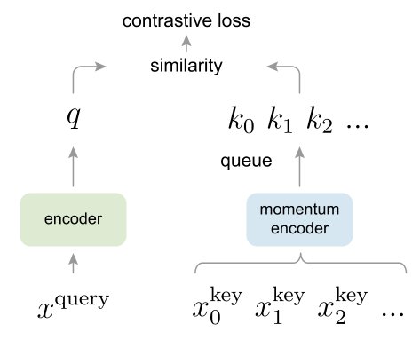
Figure 1: Momentum Contrast (MoCo) trains a visual representation encoder by matching an encoded query to a dictionary of encoded keys using a contrastive loss. The dictionary keys are defined on-the-fly by a set of data samples. The dictionary is built as a queue, with the current mini-batch enqueued and the oldest mini-batch dequeued, decoupling it from the mini-batch size. The keys are encoded by a slowly progressing encoder, driven by a momentum update with the query encoder. This method enables a large and consistent dictionary for learning visual representations.
图 1:动量对比(MoCo)用对比损失训练视觉表示编码器,使编码查询 匹配由编码键构成的词典。词典键 由一组数据样本在线定义。词典以队列形式维护:当前 mini-batch 入队、最旧 mini-batch 出队,从而与 mini-batch 大小解耦。键由缓慢推进的编码器编码,该编码器相对查询编码器做动量更新。该方法使学习视觉表示时能拥有又大又一致的词典。
We present Momentum Contrast (MoCo) as a way of building large and consistent dictionaries for unsupervised learning with a contrastive loss (Figure 1). We maintain the dictionary as a queue of data samples: the encoded representations of the current mini-batch are enqueued, and the oldest are dequeued. The queue decouples the dictionary size from the mini-batch size, allowing it to be large. Moreover, as the dictionary keys come from the preceding several mini-batches, a slowly progressing key encoder, implemented as a momentum-based moving average of the query encoder, is proposed to maintain consistency.
我们提出动量对比(MoCo),作为用对比损失做无监督学习时构建又大又一致词典的一种方式(图 1)。词典维护为数据样本的队列:当前 mini-batch 的编码表示入队,最旧的出队。队列使词典大小与 mini-batch 大小解耦,从而可以很大。此外,由于词典键来自此前若干 mini-batch,我们提出用查询编码器的动量滑动平均实现缓慢推进的键编码器,以保持一致性。
MoCo is a mechanism for building dynamic dictionaries for contrastive learning, and can be used with various pretext tasks. In this paper, we follow a simple instance discrimination task [61, 63, 2]: a query matches a key if they are encoded views (e.g., different crops) of the same image. Using this pretext task, MoCo shows competitive results under the common protocol of linear classification in the ImageNet dataset [11].
MoCo 是为对比学习构建动态词典的机制,可与多种 pretext 任务配合。本文沿用简单的实例判别任务 [61, 63, 2]:若查询与键是同一图像的不同编码视图(例如不同裁剪),则匹配。在此 pretext 下,MoCo 在 ImageNet [11] 常见线性分类协议上表现有竞争力。
A main purpose of unsupervised learning is to pre-train representations (i.e., features) that can be transferred to downstream tasks by fine-tuning. We show that in 7 downstream tasks related to detection or segmentation, MoCo unsupervised pre-training can surpass its ImageNet supervised counterpart, in some cases by nontrivial margins. In these experiments, we explore MoCo pre-trained on ImageNet or on a one-billion Instagram image set, demonstrating that MoCo can work well in a more real-world, billion-image scale, and relatively uncurated scenario. These results show that MoCo largely closes the gap between unsupervised and supervised representation learning in many computer vision tasks, and can serve as an alternative to ImageNet supervised pre-training in several applications.
无监督学习的一个主要目的是预训练可迁移到下游、经微调使用的表示(即特征)。我们表明:在 7 项与检测或分割相关的下游任务中,MoCo 无监督预训练可超过其 ImageNet 有监督对照,有时差距不小。实验中我们探索在 ImageNet 或约十亿张 Instagram 图像集上预训练 MoCo,说明它能在更接近真实世界、十亿量级且相对未精选的场景下工作良好。这些结果表明 MoCo 在许多计算机视觉任务上大幅缩小了无监督与有监督表示学习的差距,并可在若干应用中作为 ImageNet 有监督预训练的替代。
2 Related Work
2 相关工作
Unsupervised/self-supervised[^1] learning methods generally involve two aspects: pretext tasks and loss functions. The term “pretext” implies that the task being solved is not of genuine interest, but is solved only for the true purpose of learning a good data representation. Loss functions can often be investigated independently of pretext tasks. MoCo focuses on the loss function aspect. Next we discuss related studies with respect to these two aspects.
无监督/自监督[^1]学习方法通常涉及两方面:pretext 任务与损失函数。「pretext」意味着所解任务本身并非真正兴趣所在,求解它只是为了学到好的数据表示。损失函数常可与 pretext 任务分开研究。MoCo 聚焦损失层面。下面按这两方面讨论相关工作。
Loss functions.
A common way of defining a loss function is to measure the difference between a model’s prediction and a fixed target, such as reconstructing the input pixels (e.g., auto-encoders) by L1 or L2 losses, or classifying the input into pre-defined categories (e.g., eight positions [13], color bins [64]) by cross-entropy or margin-based losses. Other alternatives, as described next, are also possible.
损失函数
定义损失的常见方式是度量模型预测与固定目标的差异,例如用 L1/L2 重建输入像素(如自编码器),或用交叉熵/间隔损失把输入分到预定义类别(如八个位置 [13]、颜色箱 [64])。如下所述,也有其他选择。
Contrastive losses [29] measure the similarities of sample pairs in a representation space. Instead of matching an input to a fixed target, in contrastive loss formulations the target can vary on-the-fly during training and can be defined in terms of the data representation computed by a network [29]. Contrastive learning is at the core of several recent works on unsupervised learning [61, 46, 36, 66, 35, 56, 2], which we elaborate on later in context (Sec. 3.1).
对比损失 [29] 度量表示空间中样本对的相似度。与把输入匹配到固定目标不同,对比损失表述里目标可在训练中动态变化,并可用网络算出的数据表示来定义 [29]。对比学习是若干近期无监督学习工作 [61, 46, 36, 66, 35, 56, 2] 的核心,后文(第 3.1 节)再展开。
Adversarial losses [24] measure the difference between probability distributions. It is a widely successful technique for unsupervised data generation. Adversarial methods for representation learning are explored in [15, 16]. There are relations (see [24]) between generative adversarial networks and noise-contrastive estimation (NCE) [28].
对抗损失 [24] 度量概率分布差异,是无监督数据生成中广泛成功的技术。[15, 16] 探索了用于表示学习的对抗方法。生成对抗网络与噪声对比估计(NCE)[28] 之间存在联系(见 [24])。
Pretext tasks.
A wide range of pretext tasks have been proposed. Examples include recovering the input under some corruption, e.g., denoising auto-encoders [58], context auto-encoders [48], or cross-channel auto-encoders (colorization) [64, 65]. Some pretext tasks form pseudo-labels by, e.g., transformations of a single (“exemplar”) image [17], patch orderings [13, 45], tracking [59] or segmenting objects [47] in videos, or clustering features [3, 4].
Pretext 任务
已有大量 pretext 任务被提出。例子包括在某种损坏下恢复输入,如去噪自编码器 [58]、上下文自编码器 [48],或跨通道自编码器(着色)[64, 65]。另一些用伪标签,例如单张(「exemplar」)图像的变换 [17]、图块排序 [13, 45]、视频中的跟踪 [59] 或分割物体 [47],或对特征聚类 [3, 4]。
Contrastive learning vs. pretext tasks.
Various pretext tasks can be based on some form of contrastive loss functions. The instance discrimination method [61] is related to the exemplar-based task [17] and NCE [28]. The pretext task in contrastive predictive coding (CPC) [46] is a form of context auto-encoding [48], and in contrastive multiview coding (CMC) [56] it is related to colorization [64].
对比学习 与 pretext 任务
多种 pretext 可用某种形式的对比损失。实例判别方法 [61] 与基于 exemplar 的任务 [17] 及 NCE [28] 相关。对比预测编码(CPC)[46] 的 pretext 是一种上下文自编码 [48],对比多视图编码(CMC)[56] 则与着色 [64] 相关。
3 Method
3 方法
3.1 Contrastive Learning as Dictionary Look-up
3.1 作为词典查找的对比学习
Contrastive learning [29], and its recent developments, can be thought of as training an encoder for a dictionary look-up task, as described next.
对比学习 [29] 及其近期发展,可看作训练编码器去完成词典查找任务,如下所述。
Consider an encoded query and a set of encoded samples that are the keys of a dictionary. Assume that there is a single key (denoted as ) in the dictionary that matches. A contrastive loss [29] is a function whose value is low when is similar to its positive key and dissimilar to all other keys (considered negative keys for ). With similarity measured by dot product, a form of a contrastive loss function, called InfoNCE [46], is considered in this paper:
考虑编码查询 以及作为词典键的一组编码样本 。假设词典中有唯一键(记为 )与 匹配。对比损失 [29] 在 与正键 相似、与其他键(相对 的负键)不相似时取值较低。用点积度量相似度时,本文采用一种称为 InfoNCE [46] 的对比损失形式:
where is a temperature hyper-parameter per [61]. The sum is over one positive and negative samples. Intuitively, this loss is the log loss of a -way softmax-based classifier that tries to classify as . Contrastive loss functions can also be based on other forms [29, 59, 61, 36], such as margin-based losses and variants of NCE losses.
其中 为温度超参,取自 [61]。求和覆盖一个正样本与 个负样本。直观上,该损失是 类 softmax 分类器的对数损失,试图把 分到 。对比损失也可基于其他形式 [29, 59, 61, 36],如间隔损失与 NCE 变体。
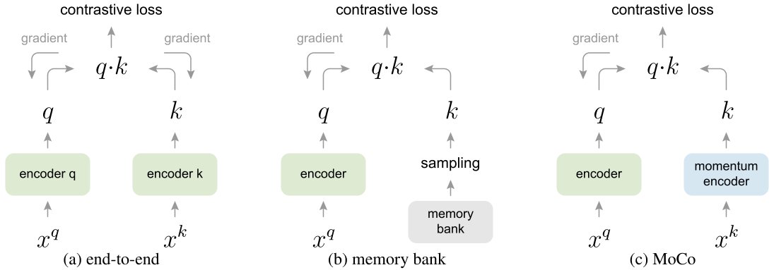
Figure 2: Conceptual comparison of three contrastive loss mechanisms (empirical comparisons are in Figure 3 and Table 3). Here we illustrate one pair of query and key. The three mechanisms differ in how the keys are maintained and how the key encoder is updated. (a): The encoders for computing the query and key representations are updated end-to-end by back-propagation (the two encoders can be different). (b): The key representations are sampled from a memory bank [61]. (c): MoCo encodes the new keys on-the-fly by a momentum-updated encoder, and maintains a queue (not illustrated in this figure) of keys.
图 2:三种对比损失机制的概念比较(经验比较见图 3 与表 3)。这里示意一对查询与键。三种机制的差别在于如何维护键、如何更新键编码器。(a):计算查询与键表示的编码器由反向传播端到端更新(两编码器可以不同)。(b):键表示从记忆库 [61] 采样。(c):MoCo 用动量更新的编码器在线编码新键,并维护键的队列(本图未画出)。
The contrastive loss serves as an unsupervised objective function for training the encoder networks that represent the queries and keys [29]. In general, the query representation is where is an encoder network and is a query sample (likewise, ). Their instantiations depend on the specific pretext task. The input and can be images [29, 61, 63], patches [46], or context consisting a set of patches [46]. The networks and can be identical [29, 59, 63], partially shared [46, 36, 2], or different [56].
对比损失作为训练表示查询与键的编码器网络的无监督目标 [29]。一般地,查询表示为 ,其中 是编码器、 是查询样本(同理 )。具体实例取决于 pretext 任务。输入 、 可以是图像 [29, 61, 63]、图块 [46],或由一组图块构成的上下文 [46]。网络 与 可以相同 [29, 59, 63]、部分共享 [46, 36, 2],或不同 [56]。
3.2 Momentum Contrast
3.2 动量对比
From the above perspective, contrastive learning is a way of building a discrete dictionary on high-dimensional continuous inputs such as images. The dictionary is dynamic in the sense that the keys are randomly sampled, and that the key encoder evolves during training. Our hypothesis is that good features can be learned by a large dictionary that covers a rich set of negative samples, while the encoder for the dictionary keys is kept as consistent as possible despite its evolution. Based on this motivation, we present Momentum Contrast as described next.
从上述视角看,对比学习是在图像这类高维连续输入上构建离散词典的一种方式。词典是动态的:键随机采样,键编码器随训练演化。我们的假设是:用大词典覆盖丰富负样本,同时尽管编码器在演化仍尽量保持键编码器一致,就能学到好特征。基于此动机,我们提出动量对比,如下。
Dictionary as a queue.
At the core of our approach is maintaining the dictionary as a queue of data samples. This allows us to reuse the encoded keys from the immediate preceding mini-batches. The introduction of a queue decouples the dictionary size from the mini-batch size. Our dictionary size can be much larger than a typical mini-batch size, and can be flexibly and independently set as a hyper-parameter.
词典作为队列
方法核心是把词典维护为数据样本的队列。这样可以复用紧邻前几个 mini-batch 编码出的键。引入队列使词典大小与 mini-batch 大小解耦:词典可以远大于典型 mini-batch,并可作为超参灵活独立设定。
The samples in the dictionary are progressively replaced. The current mini-batch is enqueued to the dictionary, and the oldest mini-batch in the queue is removed. The dictionary always represents a sampled subset of all data, while the extra computation of maintaining this dictionary is manageable. Moreover, removing the oldest mini-batch can be beneficial, because its encoded keys are the most outdated and thus the least consistent with the newest ones.
词典中的样本逐步被替换:当前 mini-batch 入队,队列中最旧的 mini-batch 移除。词典始终代表全体数据的一个采样子集,维护开销可控。移除最旧 batch 也有好处,因其编码键最过时,与最新键的一致性也最差。
Momentum update.
Using a queue can make the dictionary large, but it also makes it intractable to update the key encoder by back-propagation (the gradient should propagate to all samples in the queue). A naïve solution is to copy the key encoder from the query encoder , ignoring this gradient. But this solution yields poor results in experiments (Sec. 4.1). We hypothesize that such failure is caused by the rapidly changing encoder that reduces the key representations’ consistency. We propose a momentum update to address this issue.
动量更新
队列能让词典变大,但也使通过反向传播更新键编码器变得不可行(梯度需传到队列中所有样本)。朴素做法是把键编码器 直接复制自查询编码器 、忽略该梯度;实验中效果很差(第 4.1 节)。我们假设失败原因是编码器变化过快,降低了键表示一致性。为此提出动量更新。
Formally, denoting the parameters of as and those of as , we update by:
形式地,记 的参数为 、 的参数为 ,按下式更新 :
Here is a momentum coefficient. Only the parameters are updated by back-propagation. The momentum update in Eqn.(2) makes evolve more smoothly than . As a result, though the keys in the queue are encoded by different encoders (in different mini-batches), the difference among these encoders can be made small. In experiments, a relatively large momentum (e.g., 0.999, our default) works much better than a smaller value (e.g., ), suggesting that a slowly evolving key encoder is a core to making use of a queue.
其中 为动量系数。只有 由反向传播更新。式 (2) 的动量更新使 比 演化更平滑。因此,尽管队列中的键由不同(不同 mini-batch 的)编码器编码,这些编码器之间的差异可以很小。实验中,相对较大的动量(例如默认 )远好于较小值(例如 ),说明缓慢演化的键编码器是用好队列的核心。
Relations to previous mechanisms.
MoCo is a general mechanism for using contrastive losses. We compare it with two existing general mechanisms in Figure 2. They exhibit different properties on the dictionary size and consistency.
与先前机制的关系
MoCo 是使用对比损失的通用机制。我们在图 2 中与两种已有通用机制比较。它们在词典大小与一致性上呈现不同性质。
The end-to-end update by back-propagation is a natural mechanism (e.g., [29, 46, 36, 63, 2, 35], Figure 2a). It uses samples in the current mini-batch as the dictionary, so the keys are consistently encoded (by the same set of encoder parameters). But the dictionary size is coupled with the mini-batch size, limited by the GPU memory size. It is also challenged by large mini-batch optimization [25]. Some recent methods [46, 36, 2] are based on pretext tasks driven by local positions, where the dictionary size can be made larger by multiple positions. But these pretext tasks may require special network designs such as patchifying the input [46] or customizing the receptive field size [2], which may complicate the transfer of these networks to downstream tasks.
由反向传播做端到端更新是自然机制(例如 [29, 46, 36, 63, 2, 35],图 2a)。它用当前 mini-batch 中的样本作词典,因此键编码一致(同一组编码器参数)。但词典大小与 mini-batch 大小耦合,受 GPU 显存限制,也受大 batch 优化难题 [25] 制约。一些近期方法 [46, 36, 2] 基于由局部位置驱动的 pretext,可用多位置把词典做大;但这些任务可能需要特殊网络设计,如把输入切块 [46] 或定制感受野 [2],可能使网络向下游迁移更复杂。
Another mechanism is the memory bank approach proposed by [61] (Figure 2b). A memory bank consists of the representations of all samples in the dataset. The dictionary for each mini-batch is randomly sampled from the memory bank with no back-propagation, so it can support a large dictionary size. However, the representation of a sample in the memory bank was updated when it was last seen, so the sampled keys are essentially about the encoders at multiple different steps all over the past epoch and thus are less consistent. A momentum update is adopted on the memory bank in [61]. Its momentum update is on the representations of the same sample, not the encoder. This momentum update is irrelevant to our method, because MoCo does not keep track of every sample. Moreover, our method is more memory-efficient and can be trained on billion-scale data, which can be intractable for a memory bank.
另一种机制是 [61] 提出的记忆库(图 2b)。记忆库包含数据集中所有样本的表示;每个 mini-batch 的词典从记忆库随机采样且无反向传播,因此可支持大词典。但某样本在记忆库中的表示是在上次见到时更新的,采样出的键本质上来自过去整个 epoch 中多个不同步骤的编码器,一致性较差。[61] 也对记忆库采用动量更新,但其动量作用在同一样本的表示上,不是编码器上。该动量与我们的方法无关,因为 MoCo 不跟踪每个样本。此外,我们的方法更省内存,可在十亿级数据上训练,这对记忆库可能不可行。
Sec. 4 empirically compares these three mechanisms.
第 4 节经验比较这三种机制。
f_q, f_k: encoder networks for query and key
queue: dictionary as a queue of K keys (CxK)
m: momentum
t: temperature
f_k.params = f_q.params # initialize
for x in loader: # load a minibatch x with N samples
x_q = aug(x) # a randomly augmented version
x_k = aug(x) # another randomly augmented version
q = f_q.forward(x_q) # queries: NxC
k = f_k.forward(x_k) # keys: NxC
k = k.detach() # no gradient to keys
positive logits: Nx1
l_pos = bmm(q.view(N,1,C), k.view(N,C,1))
negative logits: NxK
l_neg = mm(q.view(N,C), queue.view(C,K))
logits: Nx(1+K)
logits = cat([l_pos, l_neg], dim=1)
contrastive loss, Eqn.(1)
labels = zeros(N) # positives are the 0-th
loss = CrossEntropyLoss(logits/t, labels)
SGD update: query network
loss.backward()
update(f_q.params)
momentum update: key network
f_k.params = m*f_k.params+(1-m)*f_q.params
update dictionary
enqueue(queue, k) # enqueue the current minibatch
dequeue(queue) # dequeue the earliest minibatch
Algorithm 1 Pseudocode of MoCo in a PyTorch-like style.
f_q, f_k: encoder networks for query and key
queue: dictionary as a queue of K keys (CxK)
m: momentum
t: temperature
f_k.params = f_q.params # initialize
for x in loader: # load a minibatch x with N samples
x_q = aug(x) # a randomly augmented version
x_k = aug(x) # another randomly augmented version
q = f_q.forward(x_q) # queries: NxC
k = f_k.forward(x_k) # keys: NxC
k = k.detach() # no gradient to keys
positive logits: Nx1
l_pos = bmm(q.view(N,1,C), k.view(N,C,1))
negative logits: NxK
l_neg = mm(q.view(N,C), queue.view(C,K))
logits: Nx(1+K)
logits = cat([l_pos, l_neg], dim=1)
contrastive loss, Eqn.(1)
labels = zeros(N) # positives are the 0-th
loss = CrossEntropyLoss(logits/t, labels)
SGD update: query network
loss.backward()
update(f_q.params)
momentum update: key network
f_k.params = m*f_k.params+(1-m)*f_q.params
update dictionary
enqueue(queue, k) # enqueue the current minibatch
dequeue(queue) # dequeue the earliest minibatch
算法 1 类 PyTorch 风格的 MoCo 伪代码。
3.3 Pretext Task
3.3 Pretext 任务
Contrastive learning can drive a variety of pretext tasks. As the focus of this paper is not on designing a new pretext task, we use a simple one mainly following the instance discrimination task in [61], to which some recent works [63, 2] are related.
对比学习可驱动多种 pretext 任务。本文重点不在设计新的 pretext,因而主要沿用 [61] 中的实例判别任务,近期若干工作 [63, 2] 也与之相关。
Following [61], we consider a query and a key as a positive pair if they originate from the same image, and otherwise as a negative sample pair. Following [63, 2], we take two random “views” of the same image under random data augmentation to form a positive pair. The queries and keys are respectively encoded by their encoders, and . The encoder can be any convolutional neural network [39].
沿用 [61],若查询与键来自同一图像则视为正对,否则为负对。沿用 [63, 2],对同一图像在随机数据增强下取两个随机「视图」构成正对。查询与键分别由其编码器 、 编码。编码器可以是任意卷积神经网络 [39]。
Algorithm 1 provides the pseudo-code of MoCo for this pretext task. For the current mini-batch, we encode the queries and their corresponding keys, which form the positive sample pairs. The negative samples are from the queue.
算法 1 给出了该 pretext 下 MoCo 的伪代码。对当前 mini-batch,我们编码查询及其对应键,构成正样本对;负样本来自队列。
Technical details.
We adopt a ResNet [33] as the encoder, whose last fully-connected layer (after global average pooling) has a fixed-dimensional output (128-D [61]). This output vector is normalized by its L2-norm [61]. This is the representation of the query or key. The temperature in Eqn.(1) is set as 0.07 [61]. The data augmentation setting follows [61]: a 224224-pixel crop is taken from a randomly resized image, and then undergoes random color jittering, random horizontal flip, and random grayscale conversion, all available in PyTorch’s torchvision package.
技术细节
编码器采用 ResNet [33],全局平均池化后的最后全连接层输出固定维(128 维 [61])。该输出向量按 L2 范数归一化 [61],即查询或键的表示。式 (1) 中温度 取 0.07 [61]。数据增强设定沿用 [61]:从随机缩放图像取 224×224 裁剪,再经随机颜色抖动、随机水平翻转与随机灰度转换,均可在 PyTorch 的 torchvision 中获得。
Shuffling BN.
Our encoders and both have Batch Normalization (BN) [37] as in the standard ResNet [33]. In experiments, we found that using BN prevents the model from learning good representations, as similarly reported in [35] (which avoids using BN). The model appears to “cheat” the pretext task and easily finds a low-loss solution. This is possibly because the intra-batch communication among samples (caused by BN) leaks information.
打乱 BN
编码器 与 都像标准 ResNet [33] 一样含 Batch Normalization(BN)[37]。实验中发现使用 BN 会妨碍学到好表示,与 [35] 的报告类似(后者干脆不用 BN)。模型似乎会「作弊」完成 pretext,轻易找到低损失解。可能原因是 BN 造成的 batch 内样本通信泄漏了信息。
We resolve this problem by shuffling BN. We train with multiple GPUs and perform BN on the samples independently for each GPU (as done in common practice). For the key encoder , we shuffle the sample order in the current mini-batch before distributing it among GPUs (and shuffle back after encoding); the sample order of the mini-batch for the query encoder is not altered. This ensures the batch statistics used to compute a query and its positive key come from two different subsets. This effectively tackles the cheating issue and allows training to benefit from BN.
我们用打乱 BN 解决该问题。训练使用多 GPU,并在每个 GPU 上独立对样本做 BN(常见做法)。对键编码器 ,在把当前 mini-batch 分到各 GPU 之前打乱样本顺序(编码后再打乱回来);查询编码器 的 mini-batch 顺序不变。这样,计算查询及其正键所用的 batch 统计来自两个不同子集,有效抑制作弊,并让训练仍能受益于 BN。
We use shuffled BN in both our method and its end-to-end ablation counterpart (Figure 2a). It is irrelevant to the memory bank counterpart (Figure 2b), which does not suffer from this issue because the positive keys are from different mini-batches in the past.
打乱 BN 用于我们的方法及其端到端消融对照(图 2a)。与记忆库对照(图 2b)无关,因后者正键来自过去不同 mini-batch,不存在该问题。
4 Experiments
4 实验
We study unsupervised training performed in:
我们研究在以下数据上的无监督训练:
ImageNet-1M(IN-1M): This is the ImageNet [11] training set that has 1.28 million images in 1000 classes (often called ImageNet-1K; we count the image number instead, as classes are not exploited by unsupervised learning). This dataset is well-balanced in its class distribution, and its images generally contain iconic view of objects.
ImageNet-1M**(IN-1M):即 ImageNet [11] 训练集,约 128 万张图、1000 类(常称 ImageNet-1K;我们按图像数计,因无监督学习不利用类别)。该集类别分布较均衡,图像多为物体的标志性视角。
Instagram-1B(IG-1B): Following [44], this is a dataset of 1 billion (940M) public images from Instagram. The images are from 1500 hashtags [44] that are related to the ImageNet categories. This dataset is relatively uncurated comparing to IN-1M, and has a long-tailed, unbalanced distribution of real-world data. This dataset contains both iconic objects and scene-level images.
Instagram-1B(IG-1B):沿用 [44],约 10 亿(940M)张来自 Instagram 的公开图像,来自与 ImageNet 类别相关的约 1500 个 hashtag [44]。相对 IN-1M 更未精选*,呈真实世界数据的*长尾、不平衡分布,既含标志性物体也含场景级图像。
Training.
We use SGD as our optimizer. The SGD weight decay is 0.0001 and the SGD momentum is 0.9. For IN-1M, we use a mini-batch size of 256 ( in Algorithm 1) in 8 GPUs, and an initial learning rate of 0.03. We train for 200 epochs with the learning rate multiplied by 0.1 at 120 and 160 epochs [61], taking 53 hours training ResNet-50. For IG-1B, we use a mini-batch size of 1024 in 64 GPUs, and a learning rate of 0.12 which is exponentially decayed by 0.9 after every 62.5k iterations (64M images). We train for 1.25M iterations (1.4 epochs of IG-1B), taking 6 days for ResNet-50.
训练
优化器用 SGD,权重衰减 0.0001,动量 0.9。IN-1M 上用 8 GPU、mini-batch 256(算法 1 中的 ),初始学习率 0.03;训 200 epoch,在第 120、160 epoch 将学习率乘 0.1 [61],ResNet-50 约需 53 小时。IG-1B 上用 64 GPU、mini-batch 1024,学习率 0.12,每 62.5k 次迭代(约 64M 图)指数衰减 0.9×;训 1.25M 次迭代(约 IG-1B 的 1.4 epoch),ResNet-50 约需 6 天。
4.1 Linear Classification Protocol
4.1 线性分类协议
We first verify our method by linear classification on frozen features, following a common protocol. In this subsection we perform unsupervised pre-training on IN-1M. Then we freeze the features and train a supervised linear classifier (a fully-connected layer followed by softmax). We train this classifier on the global average pooling features of a ResNet, for 100 epochs. We report 1-crop, top-1 classification accuracy on the ImageNet validation set.
我们先在冻结特征上用线性分类验证方法,沿用常见协议。本小节在 IN-1M 上做无监督预训练,然后冻结特征,训练有监督线性分类器(全连接层加 softmax)。在 ResNet 的全局平均池化特征上训 100 epoch,报告 ImageNet 验证集上 1-crop top-1 分类准确率。
For this classifier, we perform a grid search and find the optimal initial learning rate is 30 and weight decay is 0 (similarly reported in [56]). These hyper-parameters perform consistently well for all ablation entries presented in this subsection. These hyper-parameter values imply that the feature distributions (e.g., magnitudes) can be substantially different from those of ImageNet supervised training, an issue we will revisit in Sec. 4.2.
对该分类器做网格搜索,最优初始学习率为 30、权重衰减为 0([56] 也有类似报告)。这些超参对本小节所有消融条目表现一致。它们也暗示特征分布(例如量级)可能与 ImageNet 有监督训练明显不同,第 4.2 节会再讨论。
Ablation: contrastive loss mechanisms.
We compare the three mechanisms that are illustrated in Figure 2. To focus on the effect of contrastive loss mechanisms, we implement all of them in the same pretext task as described in Sec. 3.3. We also use the same form of InfoNCE as the contrastive loss function, Eqn.(1). As such, the comparison is solely on the three mechanisms.
消融:对比损失机制
比较图 2 所示三种机制。为聚焦机制本身,三者都实现为第 3.3 节同一 pretext,并用同一形式的 InfoNCE(式 1)作对比损失。因此比较仅针对三种机制。
The results are in Figure 3. Overall, all three mechanisms benefit from a larger . A similar trend has been observed in [61, 56] under the memory bank mechanism, while here we show that this trend is more general and can be seen in all mechanisms. These results support our motivation of building a large dictionary.
结果见图 3。总体而言,三种机制都受益于更大的 。记忆库机制下 [61, 56] 已观察到类似趋势;这里表明该趋势更一般,在所有机制中都能看到。这些结果支持我们构建大词典的动机。
The end-to-end mechanism performs similarly to MoCo when is small. However, the dictionary size is limited by the mini-batch size due to the end-to-end requirement. Here the largest mini-batch a high-end machine (8 Volta 32GB GPUs) can afford is 1024. More essentially, large mini-batch training is an open problem [25]: we found it necessary to use the linear learning rate scaling rule [25] here, without which the accuracy drops (by 2% with a 1024 mini-batch). But optimizing with a larger mini-batch is harder [25], and it is questionable whether the trend can be extrapolated into a larger even if memory is sufficient.
端到端机制在 较小时与 MoCo 相近。但因端到端要求,词典大小受 mini-batch 限制。高端机器(8 块 Volta 32GB GPU)能承受的最大 mini-batch 约为 1024。更本质的是,大 batch 训练仍是开放问题 [25]:此处必须使用线性学习率缩放规则 [25],否则准确率下降(1024 batch 时约 2%)。但更大 batch 更难优化 [25],即便显存够,趋势能否外推到更大 也存疑。
The memory bank [61] mechanism can support a larger dictionary size. But it is 2.6% worse than MoCo. This is inline with our hypothesis: the keys in the memory bank are from very different encoders all over the past epoch and they are not consistent. Note the memory bank result of 58.0% reflects our improved implementation of [61].[^2]
记忆库 [61] 机制可支持更大词典,但比 MoCo 低 2.6%。这与我们的假设一致:记忆库中的键来自过去整个 epoch 中差异很大的编码器,不够一致。注意 58.0% 的记忆库结果反映的是我们对 [61] 的改进实现。[^2]
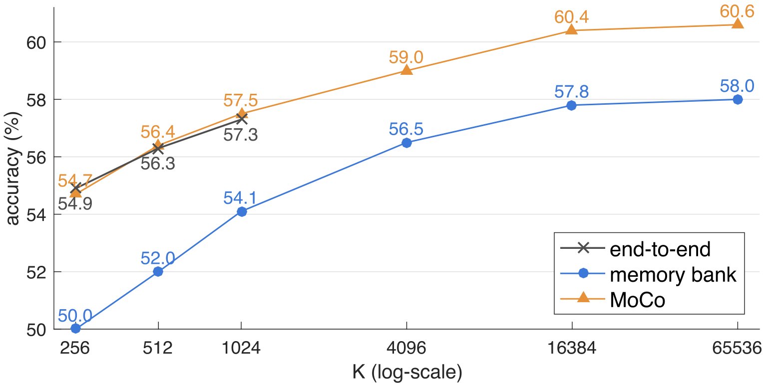
Figure 3: Comparison of three contrastive loss mechanisms under the ImageNet linear classification protocol. We adopt the same pretext task (Sec. 3.3) and only vary the contrastive loss mechanism (Figure 2). The number of negatives is in memory bank and MoCo, and is in end-to-end (offset by one because the positive key is in the same mini-batch). The network is ResNet-50.
图 3:在 ImageNet 线性分类协议下比较三种对比损失机制。采用同一 pretext(第 3.3 节),仅改变对比损失机制(图 2)。负样本数在记忆库与 MoCo 中为 ,在端到端中为 (因正键同在当前 mini-batch,故偏移 1)。网络为 ResNet-50。
Ablation: momentum.
The table below shows ResNet-50 accuracy with different MoCo momentum values ( in Eqn.(2)) used in pre-training ( 4096 here) :
消融:动量
下表给出预训练中使用不同 MoCo 动量值(式 2 中的 )时 ResNet-50 的准确率(此处 ):
It performs reasonably well when is in 0.99 0.9999, showing that a slowly progressing (i.e., relatively large momentum) key encoder is beneficial. When is too small (e.g., 0.9), the accuracy drops considerably; at the extreme of no momentum ( is 0), the training loss oscillates and fails to converge. These results support our motivation of building a consistent dictionary.
当 在 0.99 0.9999 时表现合理,说明缓慢推进(即相对较大动量)的键编码器有益。 过小(例如 0.9)时准确率明显下降;极端情况无动量()时训练损失振荡且无法收敛。这些结果支持构建一致词典的动机。
| method | architecture | #params (M) | accuracy (%) |
|---|---|---|---|
| Exemplar [17] | R50w | 211 | 46.0 [38] |
| RelativePosition [13] | R50w | 94 | 51.4 [38] |
| Jigsaw [45] | R50w | 94 | 44.6 [38] |
| Rotation [19] | Rv50w | 86 | 55.4 [38] |
| Colorization [64] | R101∗ | 28 | 39.6 [14] |
| DeepCluster [3] | VGG [53] | 15 | 48.4 [4] |
| BigBiGAN [16] | R50 | 24 | 56.6 |
| Rv50w | 86 | 61.3 | |
| methods based on contrastive learning follow: | |||
| InstDisc [61] | R50 | 24 | 54.0 |
| LocalAgg [66] | R50 | 24 | 58.8 |
| CPC v1 [46] | R101∗ | 28 | 48.7 |
| CPC v2 [35] | R170 | 303 | 65.9 |
| CMC [56] | R50 | 47 | 64.1† |
| R50w | 188 | 68.4† | |
| AMDIM [2] | AMDIM | 194 | 63.5† |
| AMDIM | 626 | 68.1† | |
| MoCo | R50 | 24 | 60.6 |
| RX50 | 46 | 63.9 | |
| R50w | 94 | 65.4 | |
| R50w | 375 | 68.6 |
Table 1: **Comparison under the linear classification protocol on ImageNet. The figure visualizes the table. All are reported as unsupervised pre-training on the ImageNet-1M training set, followed by supervised linear classification trained on frozen features, evaluated on the validation set. The parameter counts are those of the feature extractors. We compare with improved re-implementations if available (referenced after the numbers).**Notations: R101∗/R170∗ is ResNet-101/170 with the last residual stage removed [14, 46, 35], and R170 is made wider [35]; Rv50 is a reversible net [23], RX50 is ResNeXt-50-328d [62]. †: Pre-training uses FastAutoAugment [40] that is supervised by ImageNet labels.
| method | architecture | #params (M) | accuracy (%) |
|---|---|---|---|
| Exemplar [17] | R50w | 211 | 46.0 [38] |
| RelativePosition [13] | R50w | 94 | 51.4 [38] |
| Jigsaw [45] | R50w | 94 | 44.6 [38] |
| Rotation [19] | Rv50w | 86 | 55.4 [38] |
| Colorization [64] | R101∗ | 28 | 39.6 [14] |
| DeepCluster [3] | VGG [53] | 15 | 48.4 [4] |
| BigBiGAN [16] | R50 | 24 | 56.6 |
| Rv50w | 86 | 61.3 | |
| methods based on contrastive learning follow: | |||
| InstDisc [61] | R50 | 24 | 54.0 |
| LocalAgg [66] | R50 | 24 | 58.8 |
| CPC v1 [46] | R101∗ | 28 | 48.7 |
| CPC v2 [35] | R170 | 303 | 65.9 |
| CMC [56] | R50 | 47 | 64.1† |
| R50w | 188 | 68.4† | |
| AMDIM [2] | AMDIM | 194 | 63.5† |
| AMDIM | 626 | 68.1† | |
| MoCo | R50 | 24 | 60.6 |
| RX50 | 46 | 63.9 | |
| R50w | 94 | 65.4 | |
| R50w | 375 | 68.6 |
表 1:ImageNet 线性分类协议下的比较。图可视化该表。均为在 ImageNet-1M 训练集上无监督预训练,再在冻结特征上训有监督线性分类,于验证集评估。参数量为特征提取器。若有改进复现则报告之(数字后附引用)。记号:R101∗/R170∗ 为去掉最后残差阶段的 ResNet-101/170 [14, 46, 35],R170 加宽 [35];Rv50 为可逆网络 [23],RX50 为 ResNeXt-50-32×8d [62]。†:预训练使用由 ImageNet 标签监督的 FastAutoAugment [40]。
Comparison with previous results.
Previous unsupervised learning methods can differ substantially in model sizes. For a fair and comprehensive comparison, we report accuracyvs. #parameters[^3] trade-offs. Besides ResNet-50 (R50) [33], we also report its variants that are and wider (more channels), following [38].[^4] We set 65536 and 0.999. Table 1 is the comparison.
与先前结果比较
先前无监督方法在模型规模上差异很大。为公平全面比较,我们报告准确率与参数量[^3]的权衡。除 ResNet-50(R50)[33] 外,还报告按 [38] 加宽 、(更多通道)的变体。[^4]设定 、。表 1 为比较。
MoCo with R50 performs competitively and achieves 60.6% accuracy, better than all competitors of similar model sizes (24M). MoCo benefits from larger models and achieves 68.6% accuracy with R50w.
R50 上的 MoCo 有竞争力,达 60.6% 准确率,优于相近规模(约 24M)的所有竞争者。MoCo 受益于更大模型,R50w 达 68.6%。
Notably, we achieve competitive results using a standard ResNet-50 and require no specific architecture designs, e.g., patchified inputs [46, 35], carefully tailored receptive fields [2], or combining two networks [56]. By using an architecture that is not customized for the pretext task, it is easier to transfer features to a variety of visual tasks and make comparisons, studied in the next subsection.
值得一提的是,我们用标准 ResNet-50 即取得有竞争力的结果,无需为 pretext 定制结构,例如切块输入 [46, 35]、精心裁剪感受野 [2],或组合两个网络 [56]。使用不为 pretext 定制的结构,更易于把特征迁移到多种视觉任务并做比较,见下一小节。
This paper’s focus is on a mechanism for general contrastive learning; we do not explore orthogonal factors (such as specific pretext tasks) that may further improve accuracy. As an example, “MoCo v2” [8], an extension of a preliminary version of this manuscript, achieves 71.1% accuracy with R50 (up from 60.6%), given small changes on the data augmentation and output projection head [7]. We believe that this additional result shows the generality and robustness of the MoCo framework.
本文焦点是通用对比学习机制;我们不探索可能进一步抬高准确率的正交因素(如特定 pretext)。例如,「MoCo v2」[8] 作为本稿初稿的扩展,在数据增强与输出投影头上做小改动 [7] 后,R50 准确率从 60.6% 升至 71.1%。我们认为这一额外结果说明了 MoCo 框架的通用性与稳健性。
| pre-train | AP | AP | AP | |||||||||
|---|---|---|---|---|---|---|---|---|---|---|---|---|
| random init. | random init. | 64.4 | 64.4 | 37.9 | 37.9 | 38.6 | 38.6 | |||||
| random init. | ||||||||||||
| 64.4 | ||||||||||||
| 37.9 | ||||||||||||
| 38.6 | ||||||||||||
| super. IN-1M | super. | IN-1M | 81.4 | 81.4 | 54.0 | 54.0 | 59.1 | 59.1 | ||||
| super. | IN-1M | |||||||||||
| 81.4 | ||||||||||||
| 54.0 | ||||||||||||
| 59.1 | ||||||||||||
| MoCo IN-1M | MoCo | IN-1M | 81.1 (0.3) | 81.1 | (0.3) | 54.6 (0.6) | 54.6 | (0.6) | 59.9 (0.8) | 59.9 | (0.8) | |
| MoCo | IN-1M | |||||||||||
| 81.1 | (0.3) | |||||||||||
| 54.6 | (0.6) | |||||||||||
| 59.9 | (0.8) | |||||||||||
| MoCo IG-1B | MoCo | IG-1B | 81.6 (0.2) | 81.6 | (0.2) | 55.5 (1.5) | 55.5 | (1.5) | 61.2 (2.1) | 61.2 | (2.1) | |
| MoCo | IG-1B | |||||||||||
| 81.6 | (0.2) | |||||||||||
| 55.5 | (1.5) | |||||||||||
| 61.2 | (2.1) |
| random init. |
|---|
| 64.4 |
|---|
| 37.9 |
|---|
| 38.6 |
|---|
| super. | IN-1M |
|---|
| 81.4 |
|---|
| 54.0 |
|---|
| 59.1 |
|---|
| MoCo | IN-1M |
|---|
| 81.1 | (0.3) |
|---|
| 54.6 | (0.6) |
|---|
| 59.9 | (0.8) |
|---|
| MoCo | IG-1B |
|---|
| 81.6 | (0.2) |
|---|
| 55.5 | (1.5) |
|---|
| 61.2 | (2.1) |
|---|
| pre-train | AP | AP | AP | |||||||||
|---|---|---|---|---|---|---|---|---|---|---|---|---|
| random init. | random init. | 60.2 | 60.2 | 33.8 | 33.8 | 33.1 | 33.1 | |||||
| random init. | ||||||||||||
| 60.2 | ||||||||||||
| 33.8 | ||||||||||||
| 33.1 | ||||||||||||
| super. IN-1M | super. | IN-1M | 81.3 | 81.3 | 53.5 | 53.5 | 58.8 | 58.8 | ||||
| super. | IN-1M | |||||||||||
| 81.3 | ||||||||||||
| 53.5 | ||||||||||||
| 58.8 | ||||||||||||
| MoCo IN-1M | MoCo | IN-1M | 81.5 (0.2) | 81.5 | (0.2) | 55.9 (2.4) | 55.9 | (2.4) | 62.6 (3.8) | 62.6 | (3.8) | |
| MoCo | IN-1M | |||||||||||
| 81.5 | (0.2) | |||||||||||
| 55.9 | (2.4) | |||||||||||
| 62.6 | (3.8) | |||||||||||
| MoCo IG-1B | MoCo | IG-1B | 82.2 (0.9) | 82.2 | (0.9) | 57.2 (3.7) | 57.2 | (3.7) | 63.7 (4.9) | 63.7 | (4.9) | |
| MoCo | IG-1B | |||||||||||
| 82.2 | (0.9) | |||||||||||
| 57.2 | (3.7) | |||||||||||
| 63.7 | (4.9) |
| random init. |
|---|
| 60.2 |
|---|
| 33.8 |
|---|
| 33.1 |
|---|
| super. | IN-1M |
|---|
| 81.3 |
|---|
| 53.5 |
|---|
| 58.8 |
|---|
| MoCo | IN-1M |
|---|
| 81.5 | (0.2) |
|---|
| 55.9 | (2.4) |
|---|
| 62.6 | (3.8) |
|---|
| MoCo | IG-1B |
|---|
| 82.2 | (0.9) |
|---|
| 57.2 | (3.7) |
|---|
| 63.7 | (4.9) |
|---|
(a) Faster R-CNN, R50-dilated-C5
表 2a:Faster R-CNN,R50-dilated-C5(及 C4 等)在 VOC 上的结果摘要;数字与括号内相对有监督 IN-1M 的差值保持原样。
| pre-train | AP | AP | AP | |||||||||
|---|---|---|---|---|---|---|---|---|---|---|---|---|
| random init. | random init. | 64.4 | 64.4 | 37.9 | 37.9 | 38.6 | 38.6 | |||||
| random init. | ||||||||||||
| 64.4 | ||||||||||||
| 37.9 | ||||||||||||
| 38.6 | ||||||||||||
| super. IN-1M | super. | IN-1M | 81.4 | 81.4 | 54.0 | 54.0 | 59.1 | 59.1 | ||||
| super. | IN-1M | |||||||||||
| 81.4 | ||||||||||||
| 54.0 | ||||||||||||
| 59.1 | ||||||||||||
| MoCo IN-1M | MoCo | IN-1M | 81.1 (0.3) | 81.1 | (0.3) | 54.6 (0.6) | 54.6 | (0.6) | 59.9 (0.8) | 59.9 | (0.8) | |
| MoCo | IN-1M | |||||||||||
| 81.1 | (0.3) | |||||||||||
| 54.6 | (0.6) | |||||||||||
| 59.9 | (0.8) | |||||||||||
| MoCo IG-1B | MoCo | IG-1B | 81.6 (0.2) | 81.6 | (0.2) | 55.5 (1.5) | 55.5 | (1.5) | 61.2 (2.1) | 61.2 | (2.1) | |
| MoCo | IG-1B | |||||||||||
| 81.6 | (0.2) | |||||||||||
| 55.5 | (1.5) | |||||||||||
| 61.2 | (2.1) |
| random init. |
|---|
| 64.4 |
|---|
| 37.9 |
|---|
| 38.6 |
|---|
| super. | IN-1M |
|---|
| 81.4 |
|---|
| 54.0 |
|---|
| 59.1 |
|---|
| MoCo | IN-1M |
|---|
| 81.1 | (0.3) |
|---|
| 54.6 | (0.6) |
|---|
| 59.9 | (0.8) |
|---|
| MoCo | IG-1B |
|---|
| 81.6 | (0.2) |
|---|
| 55.5 | (1.5) |
|---|
| 61.2 | (2.1) |
|---|
| pre-train | AP | AP | AP | |||||||||
|---|---|---|---|---|---|---|---|---|---|---|---|---|
| random init. | random init. | 60.2 | 60.2 | 33.8 | 33.8 | 33.1 | 33.1 | |||||
| random init. | ||||||||||||
| 60.2 | ||||||||||||
| 33.8 | ||||||||||||
| 33.1 | ||||||||||||
| super. IN-1M | super. | IN-1M | 81.3 | 81.3 | 53.5 | 53.5 | 58.8 | 58.8 | ||||
| super. | IN-1M | |||||||||||
| 81.3 | ||||||||||||
| 53.5 | ||||||||||||
| 58.8 | ||||||||||||
| MoCo IN-1M | MoCo | IN-1M | 81.5 (0.2) | 81.5 | (0.2) | 55.9 (2.4) | 55.9 | (2.4) | 62.6 (3.8) | 62.6 | (3.8) | |
| MoCo | IN-1M | |||||||||||
| 81.5 | (0.2) | |||||||||||
| 55.9 | (2.4) | |||||||||||
| 62.6 | (3.8) | |||||||||||
| MoCo IG-1B | MoCo | IG-1B | 82.2 (0.9) | 82.2 | (0.9) | 57.2 (3.7) | 57.2 | (3.7) | 63.7 (4.9) | 63.7 | (4.9) | |
| MoCo | IG-1B | |||||||||||
| 82.2 | (0.9) | |||||||||||
| 57.2 | (3.7) | |||||||||||
| 63.7 | (4.9) |
| random init. |
|---|
| 60.2 |
|---|
| 33.8 |
|---|
| 33.1 |
|---|
| super. | IN-1M |
|---|
| 81.3 |
|---|
| 53.5 |
|---|
| 58.8 |
|---|
| MoCo | IN-1M |
|---|
| 81.5 | (0.2) |
|---|
| 55.9 | (2.4) |
|---|
| 62.6 | (3.8) |
|---|
| MoCo | IG-1B |
|---|
| 82.2 | (0.9) |
|---|
| 57.2 | (3.7) |
|---|
| 63.7 | (4.9) |
|---|
(a) Faster R-CNN, R50-dilated-C5
| R50-dilated-C5 | R50-C4 | ||||||
|---|---|---|---|---|---|---|---|
| pre-train | AP | AP | AP | AP | AP | AP | |
| end-to-end | 79.2 | 52.0 | 56.6 | 80.4 | 54.6 | 60.3 | |
| memory bank | 79.8 | 52.9 | 57.9 | 80.6 | 54.9 | 60.6 | |
| MoCo | 81.1 | 54.6 | 59.9 | 81.5 | 55.9 | 62.6 |
Table 3: Comparison of three contrastive loss mechanisms on PASCAL VOC object detection, fine-tuned on trainval07+12 and evaluated on test2007 (averages over 5 trials). All models are implemented by us (Figure 3), pre-trained on IN-1M, and fine-tuned using the same settings as in Table 2.
| R50-dilated-C5 | R50-C4 | ||||||
|---|---|---|---|---|---|---|---|
| pre-train | AP | AP | AP | AP | AP | AP | |
| end-to-end | 79.2 | 52.0 | 56.6 | 80.4 | 54.6 | 60.3 | |
| memory bank | 79.8 | 52.9 | 57.9 | 80.6 | 54.9 | 60.6 | |
| MoCo | 81.1 | 54.6 | 59.9 | 81.5 | 55.9 | 62.6 |
表 3:三种对比损失机制在 PASCAL VOC 目标检测上的比较,于 trainval07+12 微调、test2007 评估(5 次试验平均)。模型均由我们实现(图 3),在 IN-1M 预训练,微调设定同表 2。
| AP | AP | AP | ||||||||||||||||||||||||
|---|---|---|---|---|---|---|---|---|---|---|---|---|---|---|---|---|---|---|---|---|---|---|---|---|---|---|
| pre-train | RelPos, by [14] | Multi-task [14] | Jigsaw, by [26] | LocalAgg [66] | MoCo | MoCo | Multi-task [14] | MoCo | ||||||||||||||||||
| super. | IN-1M | 74.2 | 74.2 | 74.2 | 74.2 | 70.5 | 70.5 | 74.6 | 74.6 | 74.4 | 74.4 | 42.4 | 42.4 | 44.3 | 44.3 | 42.7 | 42.7 | |||||||||
| 74.2 | ||||||||||||||||||||||||||
| 74.2 | ||||||||||||||||||||||||||
| 70.5 | ||||||||||||||||||||||||||
| 74.6 | ||||||||||||||||||||||||||
| 74.4 | ||||||||||||||||||||||||||
| 42.4 | ||||||||||||||||||||||||||
| 44.3 | ||||||||||||||||||||||||||
| 42.7 | ||||||||||||||||||||||||||
| unsup. | IN-1M | 66.8 (7.4) | 66.8 | (7.4) | 70.5 (3.7) | 70.5 | (3.7) | 61.4 (9.1) | 61.4 | (9.1) | 69.1 (5.5) | 69.1 | (5.5) | 74.9 (0.5) | 74.9 | (0.5) | 46.6 (4.2) | 46.6 | (4.2) | 43.9 (0.4) | 43.9 | (0.4) | 50.1 (7.4) | 50.1 | (7.4) | |
| 66.8 | (7.4) | |||||||||||||||||||||||||
| 70.5 | (3.7) | |||||||||||||||||||||||||
| 61.4 | (9.1) | |||||||||||||||||||||||||
| 69.1 | (5.5) | |||||||||||||||||||||||||
| 74.9 | (0.5) | |||||||||||||||||||||||||
| 46.6 | (4.2) | |||||||||||||||||||||||||
| 43.9 | (0.4) | |||||||||||||||||||||||||
| 50.1 | (7.4) | |||||||||||||||||||||||||
| unsup. | IN-14M | - | - | - | - | 69.2 (1.3) | 69.2 | (1.3) | - | - | 75.2 (0.8) | 75.2 | (0.8) | 46.9 (4.5) | 46.9 | (4.5) | - | - | 50.2 (7.5) | 50.2 | (7.5) | |||||
| - | ||||||||||||||||||||||||||
| - | ||||||||||||||||||||||||||
| 69.2 | (1.3) | |||||||||||||||||||||||||
| - | ||||||||||||||||||||||||||
| 75.2 | (0.8) | |||||||||||||||||||||||||
| 46.9 | (4.5) | |||||||||||||||||||||||||
| - | ||||||||||||||||||||||||||
| 50.2 | (7.5) | |||||||||||||||||||||||||
| unsup. | YFCC-100M | - | - | - | - | 66.6 (3.9) | 66.6 | (3.9) | - | - | 74.7 (0.3) | 74.7 | (0.3) | 45.9 (3.5) | 45.9 | (3.5) | - | - | 49.0 (6.3) | 49.0 | (6.3) | |||||
| - | ||||||||||||||||||||||||||
| - | ||||||||||||||||||||||||||
| 66.6 | (3.9) | |||||||||||||||||||||||||
| - | ||||||||||||||||||||||||||
| 74.7 | (0.3) | |||||||||||||||||||||||||
| 45.9 | (3.5) | |||||||||||||||||||||||||
| - | ||||||||||||||||||||||||||
| 49.0 | (6.3) | |||||||||||||||||||||||||
| unsup. | IG-1B | - | - | - | - | - | - | - | - | 75.6 (1.2) | 75.6 | (1.2) | 47.6 (5.2) | 47.6 | (5.2) | - | - | 51.7 (9.0) | 51.7 | (9.0) | ||||||
| - | ||||||||||||||||||||||||||
| - | ||||||||||||||||||||||||||
| - | ||||||||||||||||||||||||||
| - | ||||||||||||||||||||||||||
| 75.6 | (1.2) | |||||||||||||||||||||||||
| 47.6 | (5.2) | |||||||||||||||||||||||||
| - | ||||||||||||||||||||||||||
| 51.7 | (9.0) |
| 74.2 |
|---|
| 74.2 |
|---|
| 70.5 |
|---|
| 74.6 |
|---|
| 74.4 |
|---|
| 42.4 |
|---|
| 44.3 |
|---|
| 42.7 |
|---|
| 66.8 | (7.4) |
|---|
| 70.5 | (3.7) |
|---|
| 61.4 | (9.1) |
|---|
| 69.1 | (5.5) |
|---|
| 74.9 | (0.5) |
|---|
| 46.6 | (4.2) |
|---|
| 43.9 | (0.4) |
|---|
| 50.1 | (7.4) |
|---|
| - |
|---|
| - |
|---|
| 69.2 | (1.3) |
|---|
| - |
|---|
| 75.2 | (0.8) |
|---|
| 46.9 | (4.5) |
|---|
| - |
|---|
| 50.2 | (7.5) |
|---|
| - |
|---|
| - |
|---|
| 66.6 | (3.9) |
|---|
| - |
|---|
| 74.7 | (0.3) |
|---|
| 45.9 | (3.5) |
|---|
| - |
|---|
| 49.0 | (6.3) |
|---|
| - |
|---|
| - |
|---|
| - |
|---|
| - |
|---|
| 75.6 | (1.2) |
|---|
| 47.6 | (5.2) |
|---|
| - |
|---|
| 51.7 | (9.0) |
|---|
Table 4: Comparison with previous methods on object detection fine-tuned on PASCAL VOC trainval2007. Evaluation is on test2007. The ImageNet supervised counterparts are from the respective papers, and are reported as having the same structure as the respective unsupervised pre-training counterparts. All entries are based on the C4 backbone. The models in [14] are R101 v2 [34], and others are R50. The RelPos (relative position) [13] result is the best single-task case in the Multi-task paper [14]. The Jigsaw [45] result is from the ResNet-based implementation in [26]. Our results are with 9k-iteration fine-tuning, averaged over 5 trials. In the brackets are the gaps to the ImageNet supervised pre-training counterpart. In green are the gaps of at least 0.5 point.
| AP | AP | AP | ||||||||||||||||||||||||
|---|---|---|---|---|---|---|---|---|---|---|---|---|---|---|---|---|---|---|---|---|---|---|---|---|---|---|
| pre-train | RelPos, by [14] | Multi-task [14] | Jigsaw, by [26] | LocalAgg [66] | MoCo | MoCo | Multi-task [14] | MoCo | ||||||||||||||||||
| super. | IN-1M | 74.2 | 74.2 | 74.2 | 74.2 | 70.5 | 70.5 | 74.6 | 74.6 | 74.4 | 74.4 | 42.4 | 42.4 | 44.3 | 44.3 | 42.7 | 42.7 | |||||||||
| 74.2 | ||||||||||||||||||||||||||
| 74.2 | ||||||||||||||||||||||||||
| 70.5 | ||||||||||||||||||||||||||
| 74.6 | ||||||||||||||||||||||||||
| 74.4 | ||||||||||||||||||||||||||
| 42.4 | ||||||||||||||||||||||||||
| 44.3 | ||||||||||||||||||||||||||
| 42.7 | ||||||||||||||||||||||||||
| unsup. | IN-1M | 66.8 (7.4) | 66.8 | (7.4) | 70.5 (3.7) | 70.5 | (3.7) | 61.4 (9.1) | 61.4 | (9.1) | 69.1 (5.5) | 69.1 | (5.5) | 74.9 (0.5) | 74.9 | (0.5) | 46.6 (4.2) | 46.6 | (4.2) | 43.9 (0.4) | 43.9 | (0.4) | 50.1 (7.4) | 50.1 | (7.4) | |
| 66.8 | (7.4) | |||||||||||||||||||||||||
| 70.5 | (3.7) | |||||||||||||||||||||||||
| 61.4 | (9.1) | |||||||||||||||||||||||||
| 69.1 | (5.5) | |||||||||||||||||||||||||
| 74.9 | (0.5) | |||||||||||||||||||||||||
| 46.6 | (4.2) | |||||||||||||||||||||||||
| 43.9 | (0.4) | |||||||||||||||||||||||||
| 50.1 | (7.4) | |||||||||||||||||||||||||
| unsup. | IN-14M | - | - | - | - | 69.2 (1.3) | 69.2 | (1.3) | - | - | 75.2 (0.8) | 75.2 | (0.8) | 46.9 (4.5) | 46.9 | (4.5) | - | - | 50.2 (7.5) | 50.2 | (7.5) | |||||
| - | ||||||||||||||||||||||||||
| - | ||||||||||||||||||||||||||
| 69.2 | (1.3) | |||||||||||||||||||||||||
| - | ||||||||||||||||||||||||||
| 75.2 | (0.8) | |||||||||||||||||||||||||
| 46.9 | (4.5) | |||||||||||||||||||||||||
| - | ||||||||||||||||||||||||||
| 50.2 | (7.5) | |||||||||||||||||||||||||
| unsup. | YFCC-100M | - | - | - | - | 66.6 (3.9) | 66.6 | (3.9) | - | - | 74.7 (0.3) | 74.7 | (0.3) | 45.9 (3.5) | 45.9 | (3.5) | - | - | 49.0 (6.3) | 49.0 | (6.3) | |||||
| - | ||||||||||||||||||||||||||
| - | ||||||||||||||||||||||||||
| 66.6 | (3.9) | |||||||||||||||||||||||||
| - | ||||||||||||||||||||||||||
| 74.7 | (0.3) | |||||||||||||||||||||||||
| 45.9 | (3.5) | |||||||||||||||||||||||||
| - | ||||||||||||||||||||||||||
| 49.0 | (6.3) | |||||||||||||||||||||||||
| unsup. | IG-1B | - | - | - | - | - | - | - | - | 75.6 (1.2) | 75.6 | (1.2) | 47.6 (5.2) | 47.6 | (5.2) | - | - | 51.7 (9.0) | 51.7 | (9.0) | ||||||
| - | ||||||||||||||||||||||||||
| - | ||||||||||||||||||||||||||
| - | ||||||||||||||||||||||||||
| - | ||||||||||||||||||||||||||
| 75.6 | (1.2) | |||||||||||||||||||||||||
| 47.6 | (5.2) | |||||||||||||||||||||||||
| - | ||||||||||||||||||||||||||
| 51.7 | (9.0) |
| 74.2 |
|---|
| 74.2 |
|---|
| 70.5 |
|---|
| 74.6 |
|---|
| 74.4 |
|---|
| 42.4 |
|---|
| 44.3 |
|---|
| 42.7 |
|---|
| 66.8 | (7.4) |
|---|
| 70.5 | (3.7) |
|---|
| 61.4 | (9.1) |
|---|
| 69.1 | (5.5) |
|---|
| 74.9 | (0.5) |
|---|
| 46.6 | (4.2) |
|---|
| 43.9 | (0.4) |
|---|
| 50.1 | (7.4) |
|---|
| - |
|---|
| - |
|---|
| 69.2 | (1.3) |
|---|
| - |
|---|
| 75.2 | (0.8) |
|---|
| 46.9 | (4.5) |
|---|
| - |
|---|
| 50.2 | (7.5) |
|---|
| - |
|---|
| - |
|---|
| 66.6 | (3.9) |
|---|
| - |
|---|
| 74.7 | (0.3) |
|---|
| 45.9 | (3.5) |
|---|
| - |
|---|
| 49.0 | (6.3) |
|---|
| - |
|---|
| - |
|---|
| - |
|---|
| - |
|---|
| 75.6 | (1.2) |
|---|
| 47.6 | (5.2) |
|---|
| - |
|---|
| 51.7 | (9.0) |
|---|
表 4:与先前方法在 PASCAL VOC 目标检测上的比较,于 trainval2007 微调、test2007 评估。有监督对照取自各文,并报告为与相应无监督预训练同结构。条目均基于 C4 骨干。[14] 中模型为 R101 v2 [34],其余为 R50。RelPos(相对位置)[13] 结果为多任务文 [14] 中最佳单任务情形。Jigsaw [45] 结果取自 [26] 的 ResNet 实现。我们的结果为 9k 次迭代微调、5 次平均。括号内为相对 ImageNet 有监督预训练对照的差距。绿色为至少 +0.5 点的差距。
4.2 Transferring Features
4.2 迁移特征
A main goal of unsupervised learning is to learn features that are transferrable. ImageNet supervised pre-training is most influential when serving as the initialization for fine-tuning in downstream tasks (e.g., [21, 20, 43, 52]). Next we compare MoCo with ImageNet supervised pre-training, transferred to various tasks including PASCAL VOC [18], COCO [42], etc. As prerequisites, we discuss two important issues involved [31]: normalization and schedules.
无监督学习的一个主要目标是学到可迁移的特征。ImageNet 有监督预训练在作为下游微调初始化时影响最大(例如 [21, 20, 43, 52])。下面把 MoCo 与 ImageNet 有监督预训练比较,迁移到 PASCAL VOC [18]、COCO [42] 等任务。作为前提,先讨论 [31] 涉及的两个重要问题:归一化与训练日程。
Normalization.
As noted in Sec. 4.1, features produced by unsupervised pre-training can have different distributions compared with ImageNet supervised pre-training. But a system for a downstream task often has hyper-parameters (e.g., learning rates) selected for supervised pre-training. To relieve this problem, we adopt feature normalization during fine-tuning: we fine-tune with BN that is trained (and synchronized across GPUs [49]), instead of freezing it by an affine layer [33]. We also use BN in the newly initialized layers (e.g., FPN [41]), which helps calibrate magnitudes.
归一化
如第 4.1 节所述,无监督预训练产生的特征分布可能与 ImageNet 有监督预训练不同。但下游系统的超参(例如学习率)常按有监督预训练选取。为缓解该问题,微调时采用特征归一化:用可训练(并跨 GPU 同步 [49])的 BN 做微调,而不是用仿射层冻结 BN [33]。新初始化层(例如 FPN [41])也使用 BN,有助于校准量级。
We perform normalization when fine-tuning supervised and unsupervised pre-training models. MoCo uses the same hyper-parameters as the ImageNet supervised counterpart.
对有监督与无监督预训练模型微调时都做归一化。MoCo 使用与 ImageNet 有监督对照相同的超参。
Schedules.
If the fine-tuning schedule is long enough, training detectors from random initialization can be strong baselines, and can match the ImageNet supervised counterpart on COCO [31]. Our goal is to investigate transferability of features, so our experiments are on controlled schedules, e.g., the 1 (12 epochs) or 2 schedules [22] for COCO, in contrast to 69 in [31]. On smaller datasets like VOC, training longer may not catch up [31].
训练日程
若微调日程足够长,从随机初始化训练检测器也可成为强基线,并在 COCO 上追上 ImageNet 有监督对照 [31]。我们的目标是考察特征可迁移性,因此实验采用受控日程,例如 COCO 的 1(约 12 epoch)或 2 日程 [22],而不是 [31] 中的 6~9。在 VOC 等较小数据集上,训更久也未必追得上 [31]。
Nonetheless, in our fine-tuning, MoCo uses the same schedule as the ImageNet supervised counterpart, and random initialization results are provided as references.
尽管如此,微调中 MoCo 使用与 ImageNet 有监督对照相同的日程,并给出随机初始化结果作参考。
Put together, our fine-tuning uses the same setting as the supervised pre-training counterpart. This may place MoCo at a disadvantage. Even so, MoCo is competitive. Doing so also makes it feasible to present comparisons on multiple datasets/tasks, without extra hyper-parameter search.
综合起来,我们的微调设定与有监督预训练对照相同。这可能使 MoCo 处于不利位置;即便如此,MoCo 仍有竞争力。这样做也便于在多数据集/任务上比较,而无需额外超参搜索。
Setup.
The detector is Faster R-CNN [52] with a backbone of R50-dilated-C5 or R50-C4 [32] (details in appendix), with BN tuned, implemented in [60]. We fine-tune all layers end-to-end. The image scale is [480, 800] pixels during training and 800 at inference. The same setup is used for all entries, including the supervised pre-training baseline. We evaluate the default VOC metric of AP (i.e., IoU threshold is 50%) and the more stringent metrics of COCO-style AP and AP. Evaluation is on the VOC test2007 set.
设定
检测器为 Faster R-CNN [52],骨干为 R50-dilated-C5 或 R50-C4 [32](细节见附录),BN 可调,实现于 [60]。端到端微调所有层。训练时图像尺度 [480, 800] 像素,推理时 800。所有条目(含有监督预训练基线)使用同一设定。评估默认 VOC 指标 AP(即 IoU 阈值为 50%)以及更严格的 COCO 风格 AP 与 AP。评估在 VOC test2007 集上。
Ablation: backbones.
Table 2 shows the results fine-tuned on trainval07+12 (16.5k images). For R50-dilated-C5 (Table 2a), MoCo pre-trained on IN-1M is comparable to the supervised pre-training counterpart, and MoCo pre-trained on IG-1B surpasses it. For R50-C4 (Table 2b), MoCo with IN-1M or IG-1B is better than the supervised counterpart: up to +0.9 AP, +3.7 AP, and +4.9 AP.
消融:骨干
表 2 给出在 trainval07+12(约 16.5k 图)上微调的结果。对 R50-dilated-C5(表 2a),IN-1M 预训练的 MoCo 与有监督对照相当,IG-1B 预训练的 MoCo 超过它。对 R50-C4(表 2b),IN-1M 或 IG-1B 的 MoCo 都优于有监督对照:最高达 +0.9 AP、+3.7 AP、+4.9 AP。
Interestingly, the transferring accuracy depends on the detector structure. For the C4 backbone, by default used in existing ResNet-based results [14, 61, 26, 66], the advantage of unsupervised pre-training is larger. The relation between pre-training vs. detector structures has been veiled in the past, and should be a factor under consideration.
有趣的是,迁移精度依赖检测器结构。对现有基于 ResNet 的结果默认使用的 C4 骨干 [14, 61, 26, 66],无监督预训练优势更大。预训练与检测器结构的关系过去被掩盖,应作为考虑因素。
Ablation: contrastive loss mechanisms.
We point out that these results are partially because we establish solid detection baselines for contrastive learning. To pin-point the gain that is solely contributed by using the MoCo mechanism in contrastive learning, we fine-tune the models pre-trained with the end-to-end or memory bank mechanism, both implemented by us (i.e., the best ones in Figure 3), using the same fine-tuning setting as MoCo.
消融:对比损失机制
我们指出这些结果部分得益于为对比学习建立了扎实的检测基线。为单独量化 MoCo 机制本身的增益,我们对端到端与记忆库机制预训练的模型(均由我们实现,即图 3 中最佳者)用与 MoCo 相同的微调设定做微调。
These competitors perform decently (Table 3). Their AP and AP with the C4 backbone are also higher than the ImageNet supervised counterpart’s, c.f. Table 2b, but other metrics are lower. They are worse than MoCo in all metrics. This shows the benefits of MoCo. In addition, how to train these competitors in larger-scale data is an open question, and they may not benefit from IG-1B.
这些竞争者表现尚可(表 3)。其在 C4 骨干上的 AP 与 AP 也高于 ImageNet 有监督对照,参见表 2b,但其他指标更低。它们在所有指标上都弱于 MoCo。这说明了 MoCo 的好处。此外,如何在更大规模数据上训练这些竞争者仍是开放问题,它们未必能受益于 IG-1B。
Comparison with previous results.
Following the competitors, we fine-tune on trainval2007 (5k images) using the C4 backbone. The comparison is in Table 4.
与先前结果比较
沿用竞争者做法,我们在 trainval2007(约 5k 图)上用 C4 骨干微调。比较见表 4。
For the AP metric, no previous method can catch up with its respective supervised pre-training counterpart. MoCo pre-trained on any of IN-1M, IN-14M (full ImageNet), YFCC-100M [55], and IG-1B can outperform the supervised baseline. Large gains are seen in the more stringent metrics: up to +5.2 AP and +9.0 AP. These gains are larger than the gains seen in trainval07+12 (Table 2b).
就 AP 而言,没有先前方法能追上各自的有监督预训练对照。在 IN-1M、IN-14M(完整 ImageNet)、YFCC-100M [55] 与 IG-1B 任一数据上预训练的 MoCo 都能超过有监督基线。更严格指标上增益更大:最高 +5.2 AP、+9.0 AP。这些增益大于 trainval07+12(表 2b)上所见。
| pre-train | AP | AP | AP | AP | AP | AP | ||||||||
|---|---|---|---|---|---|---|---|---|---|---|---|---|---|---|
| random init. | 31.0 | 49.5 | 33.2 | 28.5 | 46.8 | 30.4 | ||||||||
| super. IN-1M | 38.9 | 59.6 | 42.7 | 35.4 | 56.5 | 38.1 | ||||||||
| MoCo IN-1M | 38.5 | (0.4) | 58.9 | (0.7) | 42.0 | (0.7) | 35.1 | (0.3) | 55.9 | (0.6) | 37.7 | (0.4) | ||
| MoCo IG-1B | 38.9 | (0.0) | 59.4 | (0.2) | 42.3 | (0.4) | 35.4 | (0.0) | 56.5 | (0.0) | 37.9 | (0.2) |
| AP | AP | AP | AP | AP | AP | |||||||
|---|---|---|---|---|---|---|---|---|---|---|---|---|
| 36.7 | 56.7 | 40.0 | 33.7 | 53.8 | 35.9 | |||||||
| 40.6 | 61.3 | 44.4 | 36.8 | 58.1 | 39.5 | |||||||
| 40.8 | (0.2) | 61.6 | (0.3) | 44.7 | (0.3) | 36.9 | (0.1) | 58.4 | (0.3) | 39.7 | (0.2) | |
| 41.1 | (0.5) | 61.8 | (0.5) | 45.1 | (0.7) | 37.4 | (0.6) | 59.1 | (1.0) | 40.2 | (0.7) |
| pre-train | AP | AP | AP | AP | AP | AP | ||||||||
|---|---|---|---|---|---|---|---|---|---|---|---|---|---|---|
| random init. | 26.4 | 44.0 | 27.8 | 29.3 | 46.9 | 30.8 | ||||||||
| super. IN-1M | 38.2 | 58.2 | 41.2 | 33.3 | 54.7 | 35.2 | ||||||||
| MoCo IN-1M | 38.5 | (0.3) | 58.3 | (0.1) | 41.6 | (0.4) | 33.6 | (0.3) | 54.8 | (0.1) | 35.6 | (0.4) | ||
| MoCo IG-1B | 39.1 | (0.9) | 58.7 | (0.5) | 42.2 | (1.0) | 34.1 | (0.8) | 55.4 | (0.7) | 36.4 | (1.2) |
| AP | AP | AP | AP | AP | AP | |||||||
|---|---|---|---|---|---|---|---|---|---|---|---|---|
| 35.6 | 54.6 | 38.2 | 31.4 | 51.5 | 33.5 | |||||||
| 40.0 | 59.9 | 43.1 | 34.7 | 56.5 | 36.9 | |||||||
| 40.7 | (0.7) | 60.5 | (0.6) | 44.1 | (1.0) | 35.4 | (0.7) | 57.3 | (0.8) | 37.6 | (0.7) | |
| 41.1 | (1.1) | 60.7 | (0.8) | 44.8 | (1.7) | 35.6 | (0.9) | 57.4 | (0.9) | 38.1 | (1.2) |
(a) Mask R-CNN, R50-FPN, 1 schedule
(a) Mask R-CNN,R50-FPN,1 日程(COCO 结果表;数字保持原样)
| pre-train | AP | AP | AP | AP | AP | AP | ||||||||
|---|---|---|---|---|---|---|---|---|---|---|---|---|---|---|
| random init. | 31.0 | 49.5 | 33.2 | 28.5 | 46.8 | 30.4 | ||||||||
| super. IN-1M | 38.9 | 59.6 | 42.7 | 35.4 | 56.5 | 38.1 | ||||||||
| MoCo IN-1M | 38.5 | (0.4) | 58.9 | (0.7) | 42.0 | (0.7) | 35.1 | (0.3) | 55.9 | (0.6) | 37.7 | (0.4) | ||
| MoCo IG-1B | 38.9 | (0.0) | 59.4 | (0.2) | 42.3 | (0.4) | 35.4 | (0.0) | 56.5 | (0.0) | 37.9 | (0.2) |
| AP | AP | AP | AP | AP | AP | |||||||
|---|---|---|---|---|---|---|---|---|---|---|---|---|
| 36.7 | 56.7 | 40.0 | 33.7 | 53.8 | 35.9 | |||||||
| 40.6 | 61.3 | 44.4 | 36.8 | 58.1 | 39.5 | |||||||
| 40.8 | (0.2) | 61.6 | (0.3) | 44.7 | (0.3) | 36.9 | (0.1) | 58.4 | (0.3) | 39.7 | (0.2) | |
| 41.1 | (0.5) | 61.8 | (0.5) | 45.1 | (0.7) | 37.4 | (0.6) | 59.1 | (1.0) | 40.2 | (0.7) |
| pre-train | AP | AP | AP | AP | AP | AP | ||||||||
|---|---|---|---|---|---|---|---|---|---|---|---|---|---|---|
| random init. | 26.4 | 44.0 | 27.8 | 29.3 | 46.9 | 30.8 | ||||||||
| super. IN-1M | 38.2 | 58.2 | 41.2 | 33.3 | 54.7 | 35.2 | ||||||||
| MoCo IN-1M | 38.5 | (0.3) | 58.3 | (0.1) | 41.6 | (0.4) | 33.6 | (0.3) | 54.8 | (0.1) | 35.6 | (0.4) | ||
| MoCo IG-1B | 39.1 | (0.9) | 58.7 | (0.5) | 42.2 | (1.0) | 34.1 | (0.8) | 55.4 | (0.7) | 36.4 | (1.2) |
| AP | AP | AP | AP | AP | AP | |||||||
|---|---|---|---|---|---|---|---|---|---|---|---|---|
| 35.6 | 54.6 | 38.2 | 31.4 | 51.5 | 33.5 | |||||||
| 40.0 | 59.9 | 43.1 | 34.7 | 56.5 | 36.9 | |||||||
| 40.7 | (0.7) | 60.5 | (0.6) | 44.1 | (1.0) | 35.4 | (0.7) | 57.3 | (0.8) | 37.6 | (0.7) | |
| 41.1 | (1.1) | 60.7 | (0.8) | 44.8 | (1.7) | 35.6 | (0.9) | 57.4 | (0.9) | 38.1 | (1.2) |
(a) Mask R-CNN, R50-FPN, 1 schedule
Setup.
The model is Mask R-CNN [32] with the FPN [41] or C4 backbone, with BN tuned, implemented in [60]. The image scale is in [640, 800] pixels during training and is 800 at inference. We fine-tune all layers end-to-end. We fine-tune on the train2017 set (118k images) and evaluate on val2017. The schedule is the default 1 or 2 in [22].
设定
模型为 Mask R-CNN [32],骨干为 FPN [41] 或 C4,BN 可调,实现于 [60]。训练时图像尺度在 [640, 800] 像素,推理时 800。端到端微调所有层。在 train2017(约 118k 图)上微调,在 val2017 上评估。日程为 [22] 中默认的 1 或 2。
Results.
Table 5 shows the results on COCO with the FPN (Table 5a, b) and C4 (Table 5c, d) backbones. With the 1 schedule, all models (including the ImageNet supervised counterparts) are heavily under-trained, as indicated by the 2 points gaps to the 2 schedule cases. With the 2 schedule, MoCo is better than its ImageNet supervised counterpart in all metrics in both backbones.
结果
表 5 给出 COCO 上 FPN(表 5a, b)与 C4(表 5c, d)骨干的结果。1 日程下,所有模型(含 ImageNet 有监督对照)都明显训练不足,相对 2 约差 2 点。2 日程下,MoCo 在两种骨干的所有指标上都优于其 ImageNet 有监督对照。
| COCO keypoint detection | |||||||||||
|---|---|---|---|---|---|---|---|---|---|---|---|
| pre-train | AP | AP | AP | ||||||||
| random init. | 65.9 | 65.9 | 86.5 | 86.5 | 71.7 | 71.7 | |||||
| 65.9 | |||||||||||
| 86.5 | |||||||||||
| 71.7 | |||||||||||
| super. | IN-1M | 65.8 | 65.8 | 86.9 | 86.9 | 71.9 | 71.9 | ||||
| 65.8 | |||||||||||
| 86.9 | |||||||||||
| 71.9 | |||||||||||
| MoCo | IN-1M | 66.8 (1.0) | 66.8 | (1.0) | 87.4 (0.5) | 87.4 | (0.5) | 72.5 (0.6) | 72.5 | (0.6) | |
| 66.8 | (1.0) | ||||||||||
| 87.4 | (0.5) | ||||||||||
| 72.5 | (0.6) | ||||||||||
| MoCo | IG-1B | 66.9 (1.1) | 66.9 | (1.1) | 87.8 (0.9) | 87.8 | (0.9) | 73.0 (1.1) | 73.0 | (1.1) | |
| 66.9 | (1.1) | ||||||||||
| 87.8 | (0.9) | ||||||||||
| 73.0 | (1.1) |
| 65.9 |
|---|
| 86.5 |
|---|
| 71.7 |
|---|
| 65.8 |
|---|
| 86.9 |
|---|
| 71.9 |
|---|
| 66.8 | (1.0) |
|---|
| 87.4 | (0.5) |
|---|
| 72.5 | (0.6) |
|---|
| 66.9 | (1.1) |
|---|
| 87.8 | (0.9) |
|---|
| 73.0 | (1.1) |
|---|
| COCO dense pose estimation | |||||||||||
|---|---|---|---|---|---|---|---|---|---|---|---|
| pre-train | AP | AP | AP | ||||||||
| random init. | 39.4 | 39.4 | 78.5 | 78.5 | 35.1 | 35.1 | |||||
| 39.4 | |||||||||||
| 78.5 | |||||||||||
| 35.1 | |||||||||||
| super. | IN-1M | 48.3 | 48.3 | 85.6 | 85.6 | 50.6 | 50.6 | ||||
| 48.3 | |||||||||||
| 85.6 | |||||||||||
| 50.6 | |||||||||||
| MoCo | IN-1M | 50.1 (1.8) | 50.1 | (1.8) | 86.8 (1.2) | 86.8 | (1.2) | 53.9 (3.3) | 53.9 | (3.3) | |
| 50.1 | (1.8) | ||||||||||
| 86.8 | (1.2) | ||||||||||
| 53.9 | (3.3) | ||||||||||
| MoCo | IG-1B | 50.6 (2.3) | 50.6 | (2.3) | 87.0 (1.4) | 87.0 | (1.4) | 54.3 (3.7) | 54.3 | (3.7) | |
| 50.6 | (2.3) | ||||||||||
| 87.0 | (1.4) | ||||||||||
| 54.3 | (3.7) |
| 39.4 |
|---|
| 78.5 |
|---|
| 35.1 |
|---|
| 48.3 |
|---|
| 85.6 |
|---|
| 50.6 |
|---|
| 50.1 | (1.8) |
|---|
| 86.8 | (1.2) |
|---|
| 53.9 | (3.3) |
|---|
| 50.6 | (2.3) |
|---|
| 87.0 | (1.4) |
|---|
| 54.3 | (3.7) |
|---|
| LVIS v0.5 instance segmentation | |||||||||||
|---|---|---|---|---|---|---|---|---|---|---|---|
| pre-train | AP | AP | AP | ||||||||
| random init. | 22.5 | 22.5 | 34.8 | 34.8 | 23.8 | 23.8 | |||||
| 22.5 | |||||||||||
| 34.8 | |||||||||||
| 23.8 | |||||||||||
| super. | IN-1M† | 24.4 | 24.4 | 37.8 | 37.8 | 25.8 | 25.8 | ||||
| 24.4 | |||||||||||
| 37.8 | |||||||||||
| 25.8 | |||||||||||
| MoCo | IN-1M | 24.1 (0.3) | 24.1 | (0.3) | 37.4 (0.4) | 37.4 | (0.4) | 25.5 (0.3) | 25.5 | (0.3) | |
| 24.1 | (0.3) | ||||||||||
| 37.4 | (0.4) | ||||||||||
| 25.5 | (0.3) | ||||||||||
| MoCo | IG-1B | 24.9 (0.5) | 24.9 | (0.5) | 38.2 (0.4) | 38.2 | (0.4) | 26.4 (0.6) | 26.4 | (0.6) | |
| 24.9 | (0.5) | ||||||||||
| 38.2 | (0.4) | ||||||||||
| 26.4 | (0.6) |
| 22.5 |
|---|
| 34.8 |
|---|
| 23.8 |
|---|
| 24.4 |
|---|
| 37.8 |
|---|
| 25.8 |
|---|
| 24.1 | (0.3) |
|---|
| 37.4 | (0.4) |
|---|
| 25.5 | (0.3) |
|---|
| 24.9 | (0.5) |
|---|
| 38.2 | (0.4) |
|---|
| 26.4 | (0.6) |
|---|
| Cityscapes instance seg. | Semantic seg. (mIoU) | |||||||||||||
|---|---|---|---|---|---|---|---|---|---|---|---|---|---|---|
| pre-train | AP | AP | Cityscapes | VOC | ||||||||||
| random init. | 25.4 | 25.4 | 51.1 | 51.1 | 65.3 | 65.3 | 39.5 | 39.5 | ||||||
| 25.4 | ||||||||||||||
| 51.1 | ||||||||||||||
| 65.3 | ||||||||||||||
| 39.5 | ||||||||||||||
| super. | IN-1M | 32.9 | 32.9 | 59.6 | 59.6 | 74.6 | 74.6 | 74.4 | 74.4 | |||||
| 32.9 | ||||||||||||||
| 59.6 | ||||||||||||||
| 74.6 | ||||||||||||||
| 74.4 | ||||||||||||||
| MoCo | IN-1M | 32.3 (0.6) | 32.3 | (0.6) | 59.3 (0.3) | 59.3 | (0.3) | 75.3 (0.7) | 75.3 | (0.7) | 72.5 (1.9) | 72.5 | (1.9) | |
| 32.3 | (0.6) | |||||||||||||
| 59.3 | (0.3) | |||||||||||||
| 75.3 | (0.7) | |||||||||||||
| 72.5 | (1.9) | |||||||||||||
| MoCo | IG-1B | 32.9 (0.0) | 32.9 | (0.0) | 60.3 (0.7) | 60.3 | (0.7) | 75.5 (0.9) | 75.5 | (0.9) | 73.6 (0.8) | 73.6 | (0.8) | |
| 32.9 | (0.0) | |||||||||||||
| 60.3 | (0.7) | |||||||||||||
| 75.5 | (0.9) | |||||||||||||
| 73.6 | (0.8) |
| 25.4 |
|---|
| 51.1 |
|---|
| 65.3 |
|---|
| 39.5 |
|---|
| 32.9 |
|---|
| 59.6 |
|---|
| 74.6 |
|---|
| 74.4 |
|---|
| 32.3 | (0.6) |
|---|
| 59.3 | (0.3) |
|---|
| 75.3 | (0.7) |
|---|
| 72.5 | (1.9) |
|---|
| 32.9 | (0.0) |
|---|
| 60.3 | (0.7) |
|---|
| 75.5 | (0.9) |
|---|
| 73.6 | (0.8) |
|---|
Table 6: MoCo vs. ImageNet supervised pre-training, fine-tuned on various tasks. For each task, the same architecture and schedule are used for all entries (see appendix). In the brackets are the gaps to the ImageNet supervised pre-training counterpart. In green are the gaps of at least 0.5 point. †: this entry is with BN frozen, which improves results; see main text.
| COCO keypoint detection | |||||||||||
|---|---|---|---|---|---|---|---|---|---|---|---|
| pre-train | AP | AP | AP | ||||||||
| random init. | 65.9 | 65.9 | 86.5 | 86.5 | 71.7 | 71.7 | |||||
| 65.9 | |||||||||||
| 86.5 | |||||||||||
| 71.7 | |||||||||||
| super. | IN-1M | 65.8 | 65.8 | 86.9 | 86.9 | 71.9 | 71.9 | ||||
| 65.8 | |||||||||||
| 86.9 | |||||||||||
| 71.9 | |||||||||||
| MoCo | IN-1M | 66.8 (1.0) | 66.8 | (1.0) | 87.4 (0.5) | 87.4 | (0.5) | 72.5 (0.6) | 72.5 | (0.6) | |
| 66.8 | (1.0) | ||||||||||
| 87.4 | (0.5) | ||||||||||
| 72.5 | (0.6) | ||||||||||
| MoCo | IG-1B | 66.9 (1.1) | 66.9 | (1.1) | 87.8 (0.9) | 87.8 | (0.9) | 73.0 (1.1) | 73.0 | (1.1) | |
| 66.9 | (1.1) | ||||||||||
| 87.8 | (0.9) | ||||||||||
| 73.0 | (1.1) |
| 65.9 |
|---|
| 86.5 |
|---|
| 71.7 |
|---|
| 65.8 |
|---|
| 86.9 |
|---|
| 71.9 |
|---|
| 66.8 | (1.0) |
|---|
| 87.4 | (0.5) |
|---|
| 72.5 | (0.6) |
|---|
| 66.9 | (1.1) |
|---|
| 87.8 | (0.9) |
|---|
| 73.0 | (1.1) |
|---|
| COCO dense pose estimation | |||||||||||
|---|---|---|---|---|---|---|---|---|---|---|---|
| pre-train | AP | AP | AP | ||||||||
| random init. | 39.4 | 39.4 | 78.5 | 78.5 | 35.1 | 35.1 | |||||
| 39.4 | |||||||||||
| 78.5 | |||||||||||
| 35.1 | |||||||||||
| super. | IN-1M | 48.3 | 48.3 | 85.6 | 85.6 | 50.6 | 50.6 | ||||
| 48.3 | |||||||||||
| 85.6 | |||||||||||
| 50.6 | |||||||||||
| MoCo | IN-1M | 50.1 (1.8) | 50.1 | (1.8) | 86.8 (1.2) | 86.8 | (1.2) | 53.9 (3.3) | 53.9 | (3.3) | |
| 50.1 | (1.8) | ||||||||||
| 86.8 | (1.2) | ||||||||||
| 53.9 | (3.3) | ||||||||||
| MoCo | IG-1B | 50.6 (2.3) | 50.6 | (2.3) | 87.0 (1.4) | 87.0 | (1.4) | 54.3 (3.7) | 54.3 | (3.7) | |
| 50.6 | (2.3) | ||||||||||
| 87.0 | (1.4) | ||||||||||
| 54.3 | (3.7) |
| 39.4 |
|---|
| 78.5 |
|---|
| 35.1 |
|---|
| 48.3 |
|---|
| 85.6 |
|---|
| 50.6 |
|---|
| 50.1 | (1.8) |
|---|
| 86.8 | (1.2) |
|---|
| 53.9 | (3.3) |
|---|
| 50.6 | (2.3) |
|---|
| 87.0 | (1.4) |
|---|
| 54.3 | (3.7) |
|---|
| LVIS v0.5 instance segmentation | |||||||||||
|---|---|---|---|---|---|---|---|---|---|---|---|
| pre-train | AP | AP | AP | ||||||||
| random init. | 22.5 | 22.5 | 34.8 | 34.8 | 23.8 | 23.8 | |||||
| 22.5 | |||||||||||
| 34.8 | |||||||||||
| 23.8 | |||||||||||
| super. | IN-1M† | 24.4 | 24.4 | 37.8 | 37.8 | 25.8 | 25.8 | ||||
| 24.4 | |||||||||||
| 37.8 | |||||||||||
| 25.8 | |||||||||||
| MoCo | IN-1M | 24.1 (0.3) | 24.1 | (0.3) | 37.4 (0.4) | 37.4 | (0.4) | 25.5 (0.3) | 25.5 | (0.3) | |
| 24.1 | (0.3) | ||||||||||
| 37.4 | (0.4) | ||||||||||
| 25.5 | (0.3) | ||||||||||
| MoCo | IG-1B | 24.9 (0.5) | 24.9 | (0.5) | 38.2 (0.4) | 38.2 | (0.4) | 26.4 (0.6) | 26.4 | (0.6) | |
| 24.9 | (0.5) | ||||||||||
| 38.2 | (0.4) | ||||||||||
| 26.4 | (0.6) |
| 22.5 |
|---|
| 34.8 |
|---|
| 23.8 |
|---|
| 24.4 |
|---|
| 37.8 |
|---|
| 25.8 |
|---|
| 24.1 | (0.3) |
|---|
| 37.4 | (0.4) |
|---|
| 25.5 | (0.3) |
|---|
| 24.9 | (0.5) |
|---|
| 38.2 | (0.4) |
|---|
| 26.4 | (0.6) |
|---|
| Cityscapes instance seg. | Semantic seg. (mIoU) | |||||||||||||
|---|---|---|---|---|---|---|---|---|---|---|---|---|---|---|
| pre-train | AP | AP | Cityscapes | VOC | ||||||||||
| random init. | 25.4 | 25.4 | 51.1 | 51.1 | 65.3 | 65.3 | 39.5 | 39.5 | ||||||
| 25.4 | ||||||||||||||
| 51.1 | ||||||||||||||
| 65.3 | ||||||||||||||
| 39.5 | ||||||||||||||
| super. | IN-1M | 32.9 | 32.9 | 59.6 | 59.6 | 74.6 | 74.6 | 74.4 | 74.4 | |||||
| 32.9 | ||||||||||||||
| 59.6 | ||||||||||||||
| 74.6 | ||||||||||||||
| 74.4 | ||||||||||||||
| MoCo | IN-1M | 32.3 (0.6) | 32.3 | (0.6) | 59.3 (0.3) | 59.3 | (0.3) | 75.3 (0.7) | 75.3 | (0.7) | 72.5 (1.9) | 72.5 | (1.9) | |
| 32.3 | (0.6) | |||||||||||||
| 59.3 | (0.3) | |||||||||||||
| 75.3 | (0.7) | |||||||||||||
| 72.5 | (1.9) | |||||||||||||
| MoCo | IG-1B | 32.9 (0.0) | 32.9 | (0.0) | 60.3 (0.7) | 60.3 | (0.7) | 75.5 (0.9) | 75.5 | (0.9) | 73.6 (0.8) | 73.6 | (0.8) | |
| 32.9 | (0.0) | |||||||||||||
| 60.3 | (0.7) | |||||||||||||
| 75.5 | (0.9) | |||||||||||||
| 73.6 | (0.8) |
| 25.4 |
|---|
| 51.1 |
|---|
| 65.3 |
|---|
| 39.5 |
|---|
| 32.9 |
|---|
| 59.6 |
|---|
| 74.6 |
|---|
| 74.4 |
|---|
| 32.3 | (0.6) |
|---|
| 59.3 | (0.3) |
|---|
| 75.3 | (0.7) |
|---|
| 72.5 | (1.9) |
|---|
| 32.9 | (0.0) |
|---|
| 60.3 | (0.7) |
|---|
| 75.5 | (0.9) |
|---|
| 73.6 | (0.8) |
|---|
表 6 相关:COCO 关键点检测与 COCO dense pose 等结果(数字保持原样)。
4.2.3 More Downstream Tasks
Table 6 shows more downstream tasks (implementation details in appendix). Overall, MoCo performs competitively with ImageNet supervised pre-training:
4.2.3 更多下游任务
表 6 给出更多下游任务(实现细节见附录)。总体而言,MoCo 与 ImageNet 有监督预训练表现有竞争力:
COCO keypoint detection: supervised pre-training has no clear advantage over random initialization, whereas MoCo outperforms in all metrics.
COCO 关键点检测:有监督预训练相对随机初始化没有明显优势,而 MoCo 在所有指标上更优。
COCO dense pose estimation [1]: MoCo substantially outperforms supervised pre-training, e.g., by 3.7 points in AP, in this highly localization-sensitive task.
COCO dense pose 估计 [1]:在这一高度依赖定位的任务上,MoCo 大幅超过有监督预训练,例如 AP 高 3.7 点。
LVIS v0.5 instance segmentation [27]: this task has 1000 long-tailed distributed categories. Specifically in LVIS for the ImageNet supervised baseline, we find fine-tuning with frozen BN (24.4 AP) is better than tunable BN (details in appendix). So we compare MoCo with the better supervised pre-training variant in this task. MoCo with IG-1B surpasses it in all metrics.
LVIS v0.5 实例分割 [27]:该任务约有 1000 个长尾分布类别。具体到 LVIS 上的 ImageNet 有监督基线,我们发现冻结 BN 微调(24.4 AP)优于可调 BN(细节见附录)。因此在此任务上与更好的有监督变体比较。IG-1B 上的 MoCo 在所有指标上超过它。
Cityscapes instance segmentation [10]: MoCo with IG-1B is on par with its supervised pre-training counterpart in AP, and is higher in AP.
Cityscapes 实例分割 [10]:IG-1B 上的 MoCo 在 AP 上与有监督对照持平,在 AP 上更高。
Semantic segmentation: On Cityscapes [10], MoCo outperforms its supervised pre-training counterpart by up to 0.9 point. But on VOC semantic segmentation, MoCo is worse by at least 0.8 point, a negative case we have observed.
语义分割:在 Cityscapes [10] 上,MoCo 最多高出有监督对照 0.9 点;但在 VOC 语义分割上至少低 0.8 点,这是我们观察到的一个负面情形。
Summary.
In sum, MoCo can outperform its ImageNet supervised pre-training counterpart in 7 detection or segmentation tasks.[^5] Besides, MoCo is on par on Cityscapes instance segmentation, and lags behind on VOC semantic segmentation; we show another comparable case on iNaturalist [57] in appendix. Overall, MoCo has largely closed the gap between unsupervised and supervised representation learning in multiple vision tasks.
小结
总之,MoCo 可在 7 项检测或分割任务中超过其 ImageNet 有监督预训练对照。[^5]此外,在 Cityscapes 实例分割上持平,在 VOC 语义分割上落后;附录还给出 iNaturalist [57] 上另一可比情形。总体而言,MoCo 已在多项视觉任务上大幅缩小无监督与有监督表示学习的差距。
Remarkably, in all these tasks, MoCo pre-trained on IG-1B is consistently better than MoCo pre-trained on IN-1M. This shows that MoCo can perform well on this large-scale, relatively uncurated dataset. This represents a scenario towards real-world unsupervised learning.
值得指出的是,在所有这些任务中,IG-1B 预训练的 MoCo 一贯优于 IN-1M 预训练的 MoCo。这说明 MoCo 能在这一大规模、相对未精选的数据集上表现良好。这代表了朝向真实世界无监督学习的一种场景。
5 Discussion and Conclusion
5 讨论与结论
Our method has shown positive results of unsupervised learning in a variety of computer vision tasks and datasets. A few open questions are worth discussing. MoCo’s improvement from IN-1M to IG-1B is consistently noticeable but relatively small, suggesting that the larger-scale data may not be fully exploited. We hope an advanced pretext task will improve this. Beyond the simple instance discrimination task [61], it is possible to adopt MoCo for pretext tasks like masked auto-encoding, e.g., in language [12] and in vision [46]. We hope MoCo will be useful with other pretext tasks that involve contrastive learning.
我们的方法在多种计算机视觉任务与数据集上给出了无监督学习的正面结果。若干开放问题值得讨论。MoCo 从 IN-1M 到 IG-1B 的提升一贯可见但相对较小,说明更大规模数据可能尚未被充分利用。我们希望更先进的 pretext 能改善这一点。除简单的实例判别任务 [61] 外,也可把 MoCo 用于如掩码自编码一类的 pretext,例如语言中的 [12] 与视觉中的 [46]。希望 MoCo 也能配合其他涉及对比学习的 pretext 发挥作用。
Appendix A Appendix
附录 A
A.1 Implementation: Object detection backbones
A.1 实现:目标检测骨干
The R50-dilated-C5 and R50-C4 backbones are similar to those available in Detectron2 [60]: (i) R50-dilated-C5: the backbone includes the ResNet conv stage with a dilation of 2 and stride 1, followed by a 33 convolution (with BN) that reduces dimension to 512. The box prediction head consists of two hidden fully-connected layers. (ii) R50-C4: the backbone ends with the conv stage, and the box prediction head consists of the conv stage (including global pooling) followed by a BN layer.
R50-dilated-C5 与 R50-C4 骨干类似于 Detectron2 [60] 中可用的结构:(i) R50-dilated-C5:骨干包含膨胀为 2、步长为 1 的 ResNet conv 阶段,后接将维度降到 512 的 3×3 卷积(含 BN)。框预测头由两个隐全连接层组成。(ii) R50-C4:骨干止于 conv 阶段,框预测头由 conv 阶段(含全局池化)后接 BN 层组成。
A.2 Implementation: COCO keypoint detection
A.2 实现:COCO 关键点检测
We use Mask R-CNN (keypoint version) with R50-FPN, implemented in [60], fine-tuned on COCO train2017 and evaluated on val2017. The schedule is 2.
使用 Mask R-CNN(关键点版本)与 R50-FPN,实现于 [60],在 COCO train2017 微调、val2017 评估。日程为 2。
A.3 Implementation: COCO dense pose estimation
A.3 实现:COCO dense pose 估计
We use DensePose R-CNN [1] with R50-FPN, implemented in [60], fine-tuned on COCO train2017 and evaluated on val2017. The schedule is “s1”.
使用 DensePose R-CNN [1] 与 R50-FPN,实现于 [60],在 COCO train2017 微调、val2017 评估。日程为「s1」。
A.4 Implementation: LVIS instance segmentation
A.4 实现:LVIS 实例分割
We use Mask R-CNN with R50-FPN, fine-tuned in LVIS [27] train_v0.5 and evaluated in val_v0.5. We follow the baseline in [27] (arXiv v3 Appendix B).
使用 Mask R-CNN 与 R50-FPN,在 LVIS [27] train_v0.5 微调、val_v0.5 评估。遵循 [27](arXiv v3 附录 B)中的基线。
LVIS is a new dataset and model designs on it are to be explored. The following table includes the relevant ablations (all are averages of 5 trials):
LVIS 是较新数据集,其上的模型设计仍待探索。下表包含相关消融(均为 5 次试验平均):
A supervised pre-training baseline, end-to-end tuned but with BN frozen, has 24.4 AP. But tuning BN in this baseline leads to worse results and overfitting (this is unlike on COCO/VOC where tuning BN gives better or comparable accuracy). MoCo has 24.1 AP with IN-1M and 24.9 AP with IG-1B, both outperforming the supervised pre-training counterpart under the same tunable BN setting. Under the best individual settings, MoCo can still outperform the supervised pre-training case (24.9 vs. 24.4, as reported in Table 6 in Sec 4.2).
有监督预训练基线在端到端微调但冻结 BN 时为 24.4 AP。但在该基线上调 BN 会导致更差结果与过拟合(这与 COCO/VOC 上调 BN 更好或相当不同)。MoCo 在 IN-1M 上为 24.1 AP,在 IG-1B 上为 24.9 AP,在相同可调 BN 设定下都超过有监督对照。在各自最佳设定下,MoCo 仍可超过有监督情形(24.9 对 24.4,如表 6 第 4.2 节所报)。
A.5 Implementation: Semantic segmentation
A.5 实现:语义分割
We use an FCN-based [43] structure. The backbone consists of the convolutional layers in R50, and the 33 convolutions in conv5 blocks have dilation 2 and stride 1. This is followed by two extra 33 convolutions of 256 channels, with BN and ReLU, and then a 11 convolution for per-pixel classification. The total stride is 16 (FCN-16s [43]). We set dilation 6 in the two extra 33 convolutions, following the large field-of-view design in [6].
使用基于 FCN [43] 的结构。骨干由 R50 中的卷积层组成,conv5 块中的 3×3 卷积膨胀为 2、步长为 1。其后接两个 256 通道的额外 3×3 卷积(含 BN 与 ReLU),再接用于逐像素分类的 1×1 卷积。总步长为 16(FCN-16s [43])。两个额外 3×3 卷积的膨胀设为 6,沿用 [6] 的大感受野设计。
Training is with random scaling (by a ratio in [0.5, 2.0]), cropping, and horizontal flipping. The crop size is 513 on VOC and 769 on Cityscapes [6]. Inference is performed on the original image size. We train with mini-batch size 16 and weight decay 0.0001. Learning rate is 0.003 on VOC and is 0.01 on Cityscapes (multiplied by 0.1 at 70-th and 90-th percentile of training). For VOC, we train on the train_aug2012 set (augmented by [30], 10582 images) for 30k iterations, and evaluate on val2012. For Cityscapes, we train on the train_fine set (2975 images) for 90k iterations, and evaluate on the val set. Results are reported as averages over 5 trials.
训练采用随机缩放(比例 [0.5, 2.0])、裁剪与水平翻转。裁剪大小在 VOC 上为 513、在 Cityscapes 上为 769 [6]。推理在原始图像尺寸上进行。mini-batch 16,权重衰减 0.0001。学习率在 VOC 上为 0.003、在 Cityscapes 上为 0.01(在训练进度 70% 与 90% 百分位乘 0.1)。VOC 上在 train_aug2012(由 [30] 增强,10582 张)训 30k 次迭代,于 val2012 评估;Cityscapes 上在 train_fine(2975 张)训 90k 次迭代,于 val 评估。结果为 5 次试验平均。
A.6 iNaturalist fine-grained classification
A.6 iNaturalist 细粒度分类
In addition to the detection/segmentation experiments in the main paper, we study fine-grained classification on the iNaturalist 2018 dataset [57]. We fine-tune the pre-trained models end-to-end on the train set (437k images, 8142 classes) and evaluate on the val set. Training follows the typical ResNet implementation in PyTorch with 100 epochs. Fine-tuning has a learning rate of 0.025 (vs. 0.1 from scratch) decreased by 10 at the 70-th and 90-th percentile of training. The following is the R50 result:
除正文检测/分割实验外,我们在 iNaturalist 2018 [57] 上研究细粒度分类。在训练集(约 437k 图、8142 类)上端到端微调预训练模型,于验证集评估。训练沿用 PyTorch 中典型 ResNet 实现,100 epoch。微调学习率 0.025(从头训练为 0.1),在训练进度 70% 与 90% 百分位除以 10。以下为 R50 结果:
MoCo is 4% better than training from random initialization, and is closely comparable with its ImageNet supervised counterpart. This again shows that MoCo unsupervised pre-training is competitive.
MoCo 比随机初始化训练约高 4%,并与其 ImageNet 有监督对照接近。这再次说明 MoCo 无监督预训练具有竞争力。
A.7 Fine-tuning in ImageNet
A.7 在 ImageNet 上微调
Linear classification on frozen features (Sec. 4.1) is a common protocol of evaluating unsupervised pre-training methods. However, in practice, it is more common to fine-tune the features end-to-end in a downstream task. For completeness, the following table reports end-to-end fine-tuning results for the 1000-class ImageNet classification, compared with training from scratch (fine-tuning uses an initial learning rate of 0.03, vs. 0.1 from scratch):
在冻结特征上做线性分类(第 4.1 节)是评估无监督预训练的常见协议。但实践中更常见的是在下游任务端到端微调特征。为完整起见,下表报告 1000 类 ImageNet 分类的端到端微调结果,并与从头训练比较(微调初始学习率 0.03,从头为 0.1):
As here ImageNet is the downstream task, the case of MoCo pre-trained on IN-1M does not represent a real scenario (for reference, we report that its accuracy is 77.0% after fine-tuning). But unsupervised pre-training in the separate, unlabeled dataset of IG-1B represents a typical scenario: in this case, MoCo improves by 0.8%.
此处 ImageNet 本身是下游任务,IN-1M 上预训练的 MoCo 并不代表真实场景(供参考:微调后准确率为 77.0%)。但在单独、无标注的 IG-1B 上无监督预训练代表典型场景:此时 MoCo 提升 0.8%。
| pre-train | AP | AP | AP | AP | AP | AP | ||||||||
|---|---|---|---|---|---|---|---|---|---|---|---|---|---|---|
| random init. | 36.7 | 56.7 | 40.0 | 33.7 | 53.8 | 35.9 | ||||||||
| super. IN-1M | 40.6 | 61.3 | 44.4 | 36.8 | 58.1 | 39.5 | ||||||||
| MoCo IN-1M | 40.8 | (0.2) | 61.6 | (0.3) | 44.7 | (0.3) | 36.9 | (0.1) | 58.4 | (0.3) | 39.7 | (0.2) | ||
| MoCo IG-1B | 41.1 | (0.5) | 61.8 | (0.5) | 45.1 | (0.7) | 37.4 | (0.6) | 59.1 | (1.0) | 40.2 | (0.7) |
| AP | AP | AP | AP | AP | AP | |||||||
|---|---|---|---|---|---|---|---|---|---|---|---|---|
| 41.4 | 61.9 | 45.1 | 37.6 | 59.1 | 40.3 | |||||||
| 41.9 | 62.5 | 45.6 | 38.0 | 59.6 | 40.8 | |||||||
| 42.3 | (0.4) | 62.7 | (0.2) | 46.2 | (0.6) | 38.3 | (0.3) | 60.1 | (0.5) | 41.2 | (0.4) | |
| 42.8 | (0.9) | 63.2 | (0.7) | 47.0 | (1.4) | 38.7 | (0.7) | 60.5 | (0.9) | 41.3 | (0.5) |
(a) Mask R-CNN, R50-FPN, 2 schedule
(a) Mask R-CNN,R50-FPN,2 日程(附录表;数字保持原样)
| pre-train | AP | AP | AP | AP | AP | AP | ||||||||
|---|---|---|---|---|---|---|---|---|---|---|---|---|---|---|
| random init. | 36.7 | 56.7 | 40.0 | 33.7 | 53.8 | 35.9 | ||||||||
| super. IN-1M | 40.6 | 61.3 | 44.4 | 36.8 | 58.1 | 39.5 | ||||||||
| MoCo IN-1M | 40.8 | (0.2) | 61.6 | (0.3) | 44.7 | (0.3) | 36.9 | (0.1) | 58.4 | (0.3) | 39.7 | (0.2) | ||
| MoCo IG-1B | 41.1 | (0.5) | 61.8 | (0.5) | 45.1 | (0.7) | 37.4 | (0.6) | 59.1 | (1.0) | 40.2 | (0.7) |
| AP | AP | AP | AP | AP | AP | |||||||
|---|---|---|---|---|---|---|---|---|---|---|---|---|
| 41.4 | 61.9 | 45.1 | 37.6 | 59.1 | 40.3 | |||||||
| 41.9 | 62.5 | 45.6 | 38.0 | 59.6 | 40.8 | |||||||
| 42.3 | (0.4) | 62.7 | (0.2) | 46.2 | (0.6) | 38.3 | (0.3) | 60.1 | (0.5) | 41.2 | (0.4) | |
| 42.8 | (0.9) | 63.2 | (0.7) | 47.0 | (1.4) | 38.7 | (0.7) | 60.5 | (0.9) | 41.3 | (0.5) |
(a) Mask R-CNN, R50-FPN, 2 schedule
A.8 COCO longer fine-tuning
A.8 COCO 更长微调
In Table 5 we reported results of the 1 (12 epochs) and 2 schedules on COCO. These schedules were inherited from the original Mask R-CNN paper [32], which could be suboptimal given later advance in the field. In Table A.1, we supplement the results of a 6 schedule (72 epochs) [31] and compare with those of the 2 schedule.
表 5 报告了 COCO 上 1(约 12 epoch)与 2 日程的结果。这些日程继承自原始 Mask R-CNN 文 [32],在领域后续进展下可能并非最优。表 A.1 补充 6 日程(约 72 epoch)[31] 的结果,并与 2 比较。
We observe: (i) fine-tuning with ImageNet-supervised pre-training still has improvements (41.9 AP); (ii) training from scratch largely catches up (41.4 AP); (iii) the MoCo counterparts improve further (e.g., to 42.8 AP) and have larger gaps (e.g., +0.9 AP with 6, vs. +0.5 AP with 2). Table A.1 and Table 5 suggest that the MoCo pre-trained features can have larger advantages than the ImageNet-supervised features when fine-tuning longer.
我们观察到:(i) 有 ImageNet 有监督预训练的微调仍有提升(41.9 AP);(ii) 从头训练大幅追上(41.4 AP);(iii) MoCo 对照进一步提升(例如到 42.8 AP),且差距更大(例如 6 时 +0.9 AP,相对 2 的 +0.5)。表 A.1 与表 5 表明:微调更久时,MoCo 预训练特征相对 ImageNet 有监督特征可有更大优势。
A.9 Ablation on Shuffling BN
A.9 打乱 BN 消融
Figure A.1 provides the training curves of MoCo with or without shuffling BN: removing shuffling BN shows obvious overfitting to the pretext task: training accuracy of the pretext task (dash curve) quickly increases to 99.9%, and the kNN-based validation classification accuracy (solid curve) drops soon. This is observed for both the MoCo and end-to-end variants; the memory bank variant implicitly has different statistics for and , so avoids this issue.
图 A.1 给出有无打乱 BN 时 MoCo 的训练曲线:去掉打乱 BN 会对 pretext 明显过拟合——pretext 训练准确率(虚线)迅速升至 >99.9%,基于 kNN 的验证分类准确率(实线)很快下降。MoCo 与端到端变体均如此;记忆库变体对 与 隐式使用不同统计,因而避免该问题。
These experiments suggest that without shuffling BN, the sub-batch statistics can serve as a “signature” to tell which sub-batch the positive key is in. Shuffling BN can remove this signature and avoid such cheating.
这些实验表明:若无打乱 BN,子 batch 统计可作为「签名」泄露正键所在的子 batch。打乱 BN 可去掉该签名并避免此类作弊。
Figure A.1: Ablation of Shuffling BN. Dash: training curve of the pretext task, plotted as the accuracy of (+1)-way dictionary lookup. Solid: validation curve of a kNN-based monitor [61] (not a linear classifier) on ImageNet classification accuracy. This plot shows the first 80 epochs of training: training longer without shuffling BN overfits more.
图 A.1:打乱 BN 消融。虚线:pretext 任务训练曲线,画为 +1) 路词典查找准确率。实线:基于 kNN 的监控 [61](不是线性分类器)在 ImageNet 分类准确率上的验证曲线。本图展示前 80 个 epoch:不打乱 BN 时训更久过拟合更重。
References
参考文献
[1] Rıza Alp Güler, Natalia Neverova, and Iasonas Kokkinos. DensePose: Dense human pose estimation in the wild. In CVPR , 2018.
[2] Philip Bachman, R Devon Hjelm, and William Buchwalter. Learning representations by maximizing mutual information across views. arXiv:1906.00910 , 2019.
[3] Mathilde Caron, Piotr Bojanowski, Armand Joulin, and Matthijs Douze. Deep clustering for unsupervised learning of visual features. In ECCV , 2018.
[4] Mathilde Caron, Piotr Bojanowski, Julien Mairal, and Armand Joulin. Unsupervised pre-training of image features on non-curated data. In ICCV , 2019.
[5] Ken Chatfield, Victor Lempitsky, Andrea Vedaldi, and Andrew Zisserman. The devil is in the details: an evaluation of recent feature encoding methods. In BMVC , 2011.
[6] Liang-Chieh Chen, George Papandreou, Iasonas Kokkinos, Kevin Murphy, and Alan L Yuille. DeepLab: Semantic image segmentation with deep convolutional nets, atrous convolution, and fully connected CRFs. TPAMI , 2017.
[7] Ting Chen, Simon Kornblith, Mohammad Norouzi, and Geoffrey Hinton. A simple framework for contrastive learning of visual representations. arXiv:2002.05709 , 2020.
[8] Xinlei Chen, Haoqi Fan, Ross Girshick, and Kaiming He. Improved baselines with momentum contrastive learning. arXiv:2003.04297 , 2020.
[9] Adam Coates and Andrew Ng. The importance of encoding versus training with sparse coding and vector quantization. In ICML , 2011.
[10] Marius Cordts, Mohamed Omran, Sebastian Ramos, Timo Rehfeld, Markus Enzweiler, Rodrigo Benenson, Uwe Franke, Stefan Roth, and Bernt Schiele. The Cityscapes dataset for semantic urban scene understanding. In CVPR , 2016.
[11] Jia Deng, Wei Dong, Richard Socher, Li-Jia Li, Kai Li, and Li Fei-Fei. ImageNet: A large-scale hierarchical image database. In CVPR , 2009.
[12] Jacob Devlin, Ming-Wei Chang, Kenton Lee, and Kristina Toutanova. BERT: Pre-training of deep bidirectional transformers for language understanding. In NAACL , 2019.
[13] Carl Doersch, Abhinav Gupta, and Alexei A Efros. Unsupervised visual representation learning by context prediction. In ICCV , 2015.
[14] Carl Doersch and Andrew Zisserman. Multi-task self-supervised visual learning. In ICCV , 2017.
[15] Jeff Donahue, Philipp Krähenbühl, and Trevor Darrell. Adversarial feature learning. In ICLR , 2017.
[16] Jeff Donahue and Karen Simonyan. Large scale adversarial representation learning. arXiv:1907.02544 , 2019.
[17] Alexey Dosovitskiy, Jost Tobias Springenberg, Martin Riedmiller, and Thomas Brox. Discriminative unsupervised feature learning with convolutional neural networks. In NeurIPS , 2014.
[18] Mark Everingham, Luc Van Gool, Christopher KI Williams, John Winn, and Andrew Zisserman. The Pascal Visual Object Classes (VOC) Challenge. IJCV , 2010.
[19] Spyros Gidaris, Praveer Singh, and Nikos Komodakis. Unsupervised representation learning by predicting image rotations. In ICLR , 2018.
[20] Ross Girshick. Fast R-CNN. In ICCV , 2015.
[21] Ross Girshick, Jeff Donahue, Trevor Darrell, and Jitendra Malik. Rich feature hierarchies for accurate object detection and semantic segmentation. In CVPR , 2014.
[22] Ross Girshick, Ilija Radosavovic, Georgia Gkioxari, Piotr Dollár, and Kaiming He. Detectron, 2018.
[23] Aidan N Gomez, Mengye Ren, Raquel Urtasun, and Roger B Grosse. The reversible residual network: Backpropagation without storing activations. In NeurIPS , 2017.
[24] Ian Goodfellow, Jean Pouget-Abadie, Mehdi Mirza, Bing Xu, David Warde-Farley, Sherjil Ozair, Aaron Courville, and Yoshua Bengio. Generative adversarial nets. In NeurIPS , 2014.
[25] Priya Goyal, Piotr Dollár, Ross Girshick, Pieter Noordhuis, Lukasz Wesolowski, Aapo Kyrola, Andrew Tulloch, Yangqing Jia, and Kaiming He. Accurate, large minibatch SGD: Training ImageNet in 1 hour. arXiv:1706.02677 , 2017.
[26] Priya Goyal, Dhruv Mahajan, Abhinav Gupta, and Ishan Misra. Scaling and benchmarking self-supervised visual representation learning. In ICCV , 2019.
[27] Agrim Gupta, Piotr Dollar, and Ross Girshick. LVIS: A dataset for large vocabulary instance segmentation. In CVPR , 2019.
[28] Michael Gutmann and Aapo Hyvärinen. Noise-contrastive estimation: A new estimation principle for unnormalized statistical models. In AISTATS , 2010.
[29] Raia Hadsell, Sumit Chopra, and Yann LeCun. Dimensionality reduction by learning an invariant mapping. In CVPR , 2006.
[30] Bharath Hariharan, Pablo Arbeláez, Lubomir Bourdev, Subhransu Maji, and Jitendra Malik. Semantic contours from inverse detectors. In ICCV , 2011.
[31] Kaiming He, Ross Girshick, and Piotr Dollár. Rethinking ImageNet pre-training. In ICCV , 2019.
[32] Kaiming He, Georgia Gkioxari, Piotr Dollár, and Ross Girshick. Mask R-CNN. In ICCV , 2017.
[33] Kaiming He, Xiangyu Zhang, Shaoqing Ren, and Jian Sun. Deep residual learning for image recognition. In CVPR , 2016.
[34] Kaiming He, Xiangyu Zhang, Shaoqing Ren, and Jian Sun. Identity mappings in deep residual networks. In ECCV , 2016.
[35] Olivier J Hénaff, Ali Razavi, Carl Doersch, SM Eslami, and Aaron van den Oord. Data-efficient image recognition with contrastive predictive coding. arXiv:1905.09272 , 2019. Updated version accessed at https://openreview.net/pdf?id=rJerHlrYwH .
[36] R Devon Hjelm, Alex Fedorov, Samuel Lavoie-Marchildon, Karan Grewal, Adam Trischler, and Yoshua Bengio. Learning deep representations by mutual information estimation and maximization. In ICLR , 2019.
[37] Sergey Ioffe and Christian Szegedy. Batch normalization: Accelerating deep network training by reducing internal covariate shift. In ICML , 2015.
[38] Alexander Kolesnikov, Xiaohua Zhai, and Lucas Beyer. Revisiting self-supervised visual representation learning. In CVPR , 2019.
[39] Yann LeCun, Bernhard Boser, John S Denker, Donnie Henderson, Richard E Howard, Wayne Hubbard, and Lawrence D Jackel. Backpropagation applied to handwritten zip code recognition. Neural computation , 1989.
[40] Sungbin Lim, Ildoo Kim, Taesup Kim, Chiheon Kim, and Sungwoong Kim. Fast AutoAugment. arXiv:1905.00397 , 2019.
[41] Tsung-Yi Lin, Piotr Dollár, Ross Girshick, Kaiming He, Bharath Hariharan, and Serge Belongie. Feature pyramid networks for object detection. In CVPR , 2017.
[42] Tsung-Yi Lin, Michael Maire, Serge Belongie, James Hays, Pietro Perona, Deva Ramanan, Piotr Dollár, and C Lawrence Zitnick. Microsoft COCO: Common objects in context. In ECCV , 2014.
[43] Jonathan Long, Evan Shelhamer, and Trevor Darrell. Fully convolutional networks for semantic segmentation. In CVPR , 2015.
[44] Dhruv Mahajan, Ross Girshick, Vignesh Ramanathan, Kaiming He, Manohar Paluri, Yixuan Li, Ashwin Bharambe, and Laurens van der Maaten. Exploring the limits of weakly supervised pretraining. In ECCV , 2018.
[45] Mehdi Noroozi and Paolo Favaro. Unsupervised learning of visual representations by solving jigsaw puzzles. In ECCV , 2016.
[46] Aaron van den Oord, Yazhe Li, and Oriol Vinyals. Representation learning with contrastive predictive coding. arXiv:1807.03748 , 2018.
[47] Deepak Pathak, Ross Girshick, Piotr Dollár, Trevor Darrell, and Bharath Hariharan. Learning features by watching objects move. In CVPR , 2017.
[48] Deepak Pathak, Philipp Krahenbuhl, Jeff Donahue, Trevor Darrell, and Alexei A Efros. Context encoders: Feature learning by inpainting. In CVPR , 2016.
[49] Chao Peng, Tete Xiao, Zeming Li, Yuning Jiang, Xiangyu Zhang, Kai Jia, Gang Yu, and Jian Sun. MegDet: A large mini-batch object detector. In CVPR , 2018.
[50] Alec Radford, Karthik Narasimhan, Tim Salimans, and Ilya Sutskever. Improving language understanding by generative pre-training. 2018.
[51] Alec Radford, Jeffrey Wu, Rewon Child, David Luan, Dario Amodei, and Ilya Sutskever. Language models are unsupervised multitask learners. 2019.
[52] Shaoqing Ren, Kaiming He, Ross Girshick, and Jian Sun. Faster R-CNN: Towards real-time object detection with region proposal networks. In NeurIPS , 2015.
[53] Karen Simonyan and Andrew Zisserman. Very deep convolutional networks for large-scale image recognition. In ICLR , 2015.
[54] Josef Sivic and Andrew Zisserman. Video Google: a text retrieval approach to object matching in videos. In ICCV , 2003.
[55] Bart Thomee, David A Shamma, Gerald Friedland, Benjamin Elizalde, Karl Ni, Douglas Poland, Damian Borth, and Li-Jia Li. YFCC100M: The new data in multimedia research. Communications of the ACM , 2016.
[56] Yonglong Tian, Dilip Krishnan, and Phillip Isola. Contrastive multiview coding. arXiv:1906.05849 , 2019. Updated version accessed at https://openreview.net/pdf?id=BkgStySKPB .
[57] Grant Van Horn, Oisin Mac Aodha, Yang Song, Yin Cui, Chen Sun, Alex Shepard, Hartwig Adam, Pietro Perona, and Serge Belongie. The iNaturalist species classification and detection dataset. In CVPR , 2018.
[58] Pascal Vincent, Hugo Larochelle, Yoshua Bengio, and Pierre-Antoine Manzagol. Extracting and composing robust features with denoising autoencoders. In ICML , 2008.
[59] Xiaolong Wang and Abhinav Gupta. Unsupervised learning of visual representations using videos. In ICCV , 2015.
[60] Yuxin Wu, Alexander Kirillov, Francisco Massa, Wan-Yen Lo, and Ross Girshick. Detectron2. https://github.com/facebookresearch/detectron2 , 2019.
[61] Zhirong Wu, Yuanjun Xiong, Stella Yu, and Dahua Lin. Unsupervised feature learning via non-parametric instance discrimination. In CVPR , 2018. Updated version accessed at: https://arxiv.org/abs/1805.01978v1 .
[62] Saining Xie, Ross Girshick, Piotr Dollár, Zhuowen Tu, and Kaiming He. Aggregated residual transformations for deep neural networks. In CVPR , 2017.
[63] Mang Ye, Xu Zhang, Pong C Yuen, and Shih-Fu Chang. Unsupervised embedding learning via invariant and spreading instance feature. In CVPR , 2019.
[64] Richard Zhang, Phillip Isola, and Alexei A Efros. Colorful image colorization. In ECCV , 2016.
[65] Richard Zhang, Phillip Isola, and Alexei A Efros. Split-brain autoencoders: Unsupervised learning by cross-channel prediction. In CVPR , 2017.
[66] Chengxu Zhuang, Alex Lin Zhai, and Daniel Yamins. Local aggregation for unsupervised learning of visual embeddings. In ICCV , 2019. Additional results accessed from supplementary materials.