Searching for MobileNetV3
Searching for MobileNetV3
Abstract
摘要
We present the next generation of MobileNets based on a combination of complementary search techniques as well as a novel architecture design. MobileNetV3 is tuned to mobile phone CPUs through a combination of hardware-aware network architecture search (NAS) complemented by the NetAdapt algorithm and then subsequently improved through novel architecture advances. This paper starts the exploration of how automated search algorithms and network design can work together to harness complementary approaches improving the overall state of the art. Through this process we create two new MobileNet models for release: MobileNetV3-Large and MobileNetV3-Small which are targeted for high and low resource use cases. These models are then adapted and applied to the tasks of object detection and semantic segmentation. For the task of semantic segmentation (or any dense pixel prediction), we propose a new efficient segmentation decoder Lite Reduced Atrous Spatial Pyramid Pooling (LR-ASPP). We achieve new state of the art results for mobile classification, detection and segmentation. MobileNetV3-Large is 3.2% more accurate on ImageNet classification while reducing latency by 20% compared to MobileNetV2. MobileNetV3-Small is 6.6% more accurate compared to a MobileNetV2 model with comparable latency. MobileNetV3-Large detection is over 25% faster at roughly the same accuracy as MobileNetV2 on COCO detection. MobileNetV3-Large LR-ASPP is 34% faster than MobileNetV2 R-ASPP at similar accuracy for Cityscapes segmentation.
我们基于互补的搜索技术以及新的结构设计,给出下一代 MobileNet。MobileNetV3 面向手机 CPU 调参:先做面向硬件的神经结构搜索(NAS),再用 NetAdapt 算法加以补充,随后通过新的结构改进继续提升。本文开始探讨自动搜索算法与网络设计如何协同工作,把互补途径结合起来,从而推动整体水平。沿这条路径,我们发布两个新的 MobileNet 模型:面向高资源和低资源场景的 MobileNetV3-Large 与 MobileNetV3-Small。这两个模型再被改编并用于目标检测和语义分割。对于语义分割(或任何稠密像素预测),我们提出一种新的高效分割解码器 Lite Reduced Atrous Spatial Pyramid Pooling(LR-ASPP)。我们在移动端分类、检测和分割上取得了新的当时最优结果。与 MobileNetV2 相比,MobileNetV3-Large 在 ImageNet 分类上高 3.2 个百分点,同时延迟降低 20%。与延迟相当的 MobileNetV2 模型相比,MobileNetV3-Small 高 6.6 个百分点。在 COCO 检测上,MobileNetV3-Large 在精度大致相当的情况下比 MobileNetV2 快 25% 以上。在 Cityscapes 分割上,MobileNetV3-Large LR-ASPP 在相近精度下比 MobileNetV2 R-ASPP 快 34%。
- Introduction
Efficient neural networks are becoming ubiquitous in mobile applications enabling entirely new on-device experiences. They are also a key enabler of personal privacy allowing a user to gain the benefits of neural networks without needing to send their data to the server to be evaluated. Advances in neural network efficiency not only improve user experience via higher accuracy and lower latency, but also help preserve battery life through reduced power consumption.
高效神经网络正在移动应用中变得无处不在,并带来全新的端上体验。它们也是个人隐私的重要使能因素:用户可以享用神经网络的好处,而不必把数据送到服务器上再评估。神经网络效率的提升不仅通过更高精度和更低延迟改善用户体验,还通过降低功耗帮助延长电池寿命。
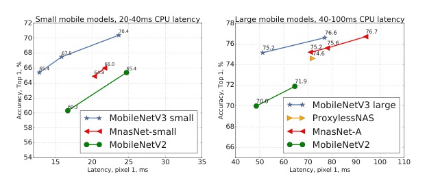
Figure 1. The trade-off between Pixel 1 latency and top-1 ImageNet accuracy. All models use the input resolution 224. V3 large and V3 small use multipliers 0.75, 1 and 1.25 to show optimal frontier. All latencies were measured on a single large core of the same device using TFLite[1]. MobileNetV3-Small and Large are our proposed next-generation mobile models.
图 1:Pixel 1 延迟与 ImageNet top-1 精度之间的权衡。所有模型的输入分辨率均为 224。V3 large 和 V3 small 使用乘数 0.75、1 和 1.25 以展示最优前沿。所有延迟均在同一设备的单颗大核上用 TFLite[1] 测得。MobileNetV3-Small 和 Large 是我们提出的下一代移动模型。
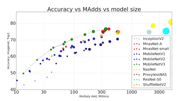
Figure 2. The trade-off between MAdds and top-1 accuracy. This allows to compare models that were targeted different hardware or software frameworks. All MobileNetV3 are for input resolution 224 and use multipliers 0.35, 0.5, 0.75, 1 and 1.25. See section 6 for other resolutions. Best viewed in color.
图 2:乘加次数(MAdds)与 top-1 精度之间的权衡。这便于比较面向不同硬件或软件框架的模型。所有 MobileNetV3 的输入分辨率均为 224,并使用乘数 0.35、0.5、0.75、1 和 1.25。其他分辨率见第 6 节。建议彩色查看。
This paper describes the approach we took to develop MobileNetV3 Large and Small models in order to deliver the next generation of high accuracy efficient neural network models to power on-device computer vision. The new networks push the state of the art forward and demonstrate how to blend automated search with novel architecture advances to build effective models.
本文介绍我们开发 MobileNetV3 Large 和 Small 模型的途径,目的是交出下一代高精度、高效率的神经网络,为端上计算机视觉提供动力。新网络把当时的水平向前推进,并展示了如何把自动搜索与新的结构改进结合起来,以构建有效的模型。
The goal of this paper is to develop the best possible mobile computer vision architectures optimizing the accuracy-latency trade off on mobile devices. To accomplish this we introduce (1) complementary search techniques, (2) new efficient versions of nonlinearities practical for the mobile setting, (3) new efficient network design, (4) a new efficient segmentation decoder. We present thorough experiments demonstrating the efficacy and value of each technique evaluated on a wide range of use cases and mobile phones.
本文的目标是开发尽可能好的移动计算机视觉结构,优化移动设备上的精度–延迟权衡。为此我们引入:(1) 互补的搜索技术;(2) 适合移动场景的新型高效非线性;(3) 新的高效网络设计;(4) 一种新的高效分割解码器。我们给出充分的实验,在多种用例和多款手机上评估每一种技术的效果与价值。
The paper is organized as follows. We start with a discussion of related work in Section 2. Section 3 reviews the efficient building blocks used for mobile models. Section 4 reviews architecture search and the complementary nature of MnasNet and NetAdapt algorithms. Section 5 describes novel architecture design improving on the efficiency of the models found through the joint search. Section 6 presents extensive experiments for classification, detection and segmentation in order do demonstrate efficacy and understand the contributions of different elements. Section 7 contains conclusions and future work.
本文组织如下。我们先在第 2 节讨论相关工作。第 3 节回顾移动模型所用的高效基本模块。第 4 节回顾结构搜索,以及 MnasNet 与 NetAdapt 算法的互补性。第 5 节描述新的结构设计,用以进一步提升联合搜索得到的模型效率。第 6 节给出分类、检测和分割上的大量实验,以展示效果并理解不同要素的贡献。第 7 节是结论与未来工作。
- Related Work
Designing deep neural network architecture for the optimal trade-off between accuracy and efficiency has been an active research area in recent years. Both novel hand-crafted structures and algorithmic neural architecture search have played important roles in advancing this field.
设计深度神经网络结构以在精度和效率之间取得最优权衡,是近年来活跃的研究方向。新颖的手工结构与算法化的神经结构搜索,都在推动这一领域前进中发挥了重要作用。
SqueezeNet[22] extensively uses 1x1 convolutions with squeeze and expand modules primarily focusing on reducing the number of parameters. More recent works shifts the focus from reducing parameters to reducing the number of operations (MAdds) and the actual measured latency. MobileNetV1[19] employs depthwise separable convolution to substantially improve computation efficiency. MobileNetV2[39] expands on this by introducing a resource-efficient block with inverted residuals and linear bottlenecks. ShuffleNet[49] utilizes group convolution and channel shuffle operations to further reduce the MAdds. CondenseNet[21] learns group convolutions at the training stage to keep useful dense connections between layers for feature re-use. ShiftNet[46] proposes the shift operation interleaved with point-wise convolutions to replace expensive spatial convolutions.
SqueezeNet[22] 大量使用带 squeeze 与 expand 模块的 1x1 卷积,主要着眼于减少参数量。更新近的工作则把重点从减少参数转向减少运算次数(MAdds)以及实际测得的延迟。MobileNetV1[19] 采用深度可分离卷积,大幅提高计算效率。MobileNetV2[39] 在此基础上引入带倒残差和线性瓶颈的资源高效模块。ShuffleNet[49] 利用分组卷积和通道混洗进一步减少 MAdds。CondenseNet[21] 在训练阶段学习分组卷积,以保留层间有用的稠密连接来复用特征。ShiftNet[46] 提出与逐点卷积交错的 shift 操作,以替代昂贵的空间卷积。
To automate the architecture design process, reinforcement learning (RL) was first introduced to search efficient architectures with competitive accuracy [53, 54, 3, 27, 35]. A fully configurable search space can grow exponentially large and intractable. So early works of architecture search focus on the cell level structure search, and the same cell is reused in all layers. Recently, [43] explored a block-level hierarchical search space allowing different layer structures at different resolution blocks of a network. To reduce the computational cost of search, differentiable architecture search framework is used in [28, 5, 45] with gradient-based optimization. Focusing on adapting existing networks to constrained mobile platforms, [48, 15, 12] proposed more efficient automated network simplification algorithms.
为了自动完成结构设计,强化学习(RL)最早被引入,用于搜索精度有竞争力的高效结构 [53, 54, 3, 27, 35]。完全可配置的搜索空间会指数级膨胀,以至难以处理。因此早期的结构搜索工作集中在细胞级结构,并在所有层中复用同一个细胞。最近,[43] 探索了块级分层搜索空间,允许网络不同分辨率块采用不同的层结构。为降低搜索的计算代价,[28, 5, 45] 采用基于梯度优化的可微分结构搜索框架。着眼于把已有网络适配到受约束的移动平台,[48, 15, 12] 提出了更高效的自动网络简化算法。
Quantization [23, 25, 47, 41, 51, 52, 37] is another important complementary effort to improve the network efficiency through reduced precision arithmetic. Finally, knowledge distillation [4, 17] offers an additional complementary method to generate small accurate "student" networks with the guidance of a large "teacher" network.
量化 [23, 25, 47, 41, 51, 52, 37] 是另一项重要的互补工作,通过降低算术精度来提高网络效率。最后,知识蒸馏 [4, 17] 提供了又一种互补方法:在大型“教师”网络的指导下,生成既小又准的“学生”网络。
- Efficient Mobile Building Blocks
Mobile models have been built on increasingly more efficient building blocks. MobileNetV1 [19] introduced depthwise separable convolutions as an efficient replacement for traditional convolution layers. Depthwise separable convolutions effectively factorize traditional convolution by separating spatial filtering from the feature generation mechanism. Depthwise separable convolutions are defined by two separate layers: light weight depthwise convolution for spatial filtering and heavier 1x1 pointwise convolutions for feature generation.
移动模型是建立在越来越高效的基本模块之上的。MobileNetV1 [19] 引入深度可分离卷积,作为传统卷积层的高效替代。深度可分离卷积通过把空间滤波与特征生成机制分开,有效地分解了传统卷积。它由两个独立的层定义:用于空间滤波的轻量深度卷积,以及用于特征生成、相对更重的 1x1 逐点卷积。
MobileNetV2 [39] introduced the linear bottleneck and inverted residual structure in order to make even more efficient layer structures by leveraging the low rank nature of the problem. This structure is shown on Figure 3 and is defined by a 1x1 expansion convolution followed by depthwise convolutions and a 1x1 projection layer. The input and output are connected with a residual connection if and only if they have the same number of channels. This structure maintains a compact representation at the input and the output while expanding to a higher-dimensional feature space internally to increase the expressiveness of nonlinear per-channel transformations.
MobileNetV2 [39] 引入线性瓶颈和倒残差结构,以利用问题的低秩性质,得到更高效的层结构。该结构见图 3,定义为一次 1x1 扩展卷积,随后是深度卷积和一次 1x1 投影层。输入与输出当且仅当通道数相同时用残差连接。这一结构在输入和输出端保持紧凑表示,同时在内部扩展到更高维的特征空间,以增强逐通道非线性变换的表达能力。
MnasNet [43] built upon the MobileNetV2 structure by introducing lightweight attention modules based on squeeze and excitation into the bottleneck structure. Note that the squeeze and excitation module are integrated in a different location than ResNet based modules proposed in [20]. The module is placed after the depthwise filters in the expansion in order for attention to be applied on the largest representation as shown on Figure 4.
MnasNet [43] 在 MobileNetV2 结构的基础上,把基于 squeeze-and-excitation 的轻量注意力模块引入瓶颈结构。需要注意,squeeze-and-excitation 模块的放置位置与 [20] 中基于 ResNet 的模块不同。该模块放在扩展部分的深度滤波之后,以便在最大的表示上施加注意力,如图 4 所示。
For MobileNetV3, we use a combination of these layers as building blocks in order to build the most effective models. Layers are also upgraded with modified swish nonlinearities [36, 13, 16]. Both squeeze and excitation as well as the swish nonlinearity use the sigmoid which can be inefficient to compute as well challenging to maintain accuracy in fixed point arithmetic so we replace this with the hard sigmoid [2, 11] as discussed in section 5.2.
对 MobileNetV3,我们把这些层组合起来作为基本模块,以构建最有效的模型。各层还升级为改进的 swish 非线性 [36, 13, 16]。squeeze-and-excitation 以及 swish 非线性都使用 sigmoid,它计算起来可能效率不高,在定点运算中也难以保持精度,因此我们按第 5.2 节的讨论,把它换成硬 sigmoid [2, 11]。
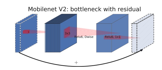
Figure 3. MobileNetV2 [39] layer (Inverted Residual and Linear Bottleneck). Each block consists of narrow input and output (bottleneck), which don't have nonlinearity, followed by expansion to a much higher-dimensional space and projection to the output. The residual connects bottleneck (rather than expansion).
图 3:MobileNetV2 [39] 的层(倒残差与线性瓶颈)。每个块由较窄的输入和输出(瓶颈)组成,瓶颈处没有非线性,随后扩展到高得多的维数空间,再投影到输出。残差连接的是瓶颈(而不是扩展部分)。
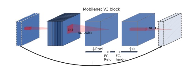
Figure 4. MobileNetV2 + Squeeze-and-Excite [20]. In contrast with [20] we apply the squeeze and excite in the residual layer. We use different nonlinearity depending on the layer, see section 5.2 for details.
图 4:MobileNetV2 + Squeeze-and-Excite [20]。与 [20] 不同,我们把 squeeze-and-excite 放在残差层中。非线性随层而异,细节见第 5.2 节。
- Network Search
Network search has shown itself to be a very powerful tool for discovering and optimizing network architectures [53, 43, 5, 48]. For MobileNetV3 we use platform-aware NAS to search for the global network structures by optimizing each network block. We then use the NetAdapt algorithm to search per layer for the number of filters. These techniques are complementary and can be combined to effectively find optimized models for a given hardware platform.
网络搜索已被证明是发现和优化网络结构的有力工具 [53, 43, 5, 48]。对 MobileNetV3,我们用面向平台的 NAS,通过优化每个网络块来搜索全局结构,再用 NetAdapt 算法按层搜索滤波器数量。这些技术是互补的,可以结合起来,为给定硬件平台有效地找到优化模型。
4.1. Platform-Aware NAS for Block-wise Search
Similar to [43], we employ a platform-aware neural architecture approach to find the global network structures. Since we use the same RNN-based controller and the same factorized hierarchical search space, we find similar results as [43] for Large mobile models with target latency around 80ms. Therefore, we simply reuse the same MnasNet-A1 [43] as our initial Large mobile model, and then apply NetAdapt [48] and other optimizations on top of it.
与 [43] 类似,我们采用面向平台的神经结构方法来寻找全局网络结构。由于使用相同的基于 RNN 的控制器和相同的分解分层搜索空间,对于目标延迟约 80ms 的大型移动模型,我们得到了与 [43] 相近的结果。因此,我们直接复用同一个 MnasNet-A1 [43] 作为最初的大型移动模型,再在其上应用 NetAdapt [48] 及其他优化。
However, we observe the original reward design is not optimized for small mobile models. Specifically, it uses a multi-objective reward to approximate Pareto-optimal solutions, by balancing model accuracy and latency for each model based on the target latency . We observe that accuracy changes much more dramatically with latency for small models; therefore, we need a smaller weight factor (vs the original in [43]) to compensate for the larger accuracy change for different latencies. Enhanced with this new weight factor , we start a new architecture search from scratch to find the initial seed model and then apply NetAdapt and other optimizations to obtain the final MobileNetV3-Small model.
不过我们观察到,原来的奖励设计并没有针对小型移动模型做优化。具体而言,它使用多目标奖励 ,根据目标延迟 来平衡每个模型 的精度 与延迟 ,以逼近帕累托最优解。我们观察到,对小模型而言,精度随延迟的变化要剧烈得多;因此需要更小的权重因子 (相对 [43] 中原来的 ),以补偿不同延迟下更大的精度变化。借助这一新的权重因子 ,我们从头开始新的结构搜索以找到初始种子模型,再应用 NetAdapt 及其他优化,得到最终的 MobileNetV3-Small 模型。
4.2. NetAdapt for Layer-wise Search
The second technique that we employ in our architecture search is NetAdapt [48]. This approach is complimentary to platform-aware NAS: it allows fine-tuning of individual layers in a sequential manner, rather than trying to infer coarse but global architecture. We refer to the original paper for the full details. In short the technique proceeds as follows:
我们在结构搜索中采用的第二种技术是 NetAdapt [48]。这一途径与面向平台的 NAS 是互补的:它允许按顺序微调单个层,而不是试图推断粗略但全局的结构。完整细节请参阅原论文。简言之,该技术按如下步骤进行:
- Starts with a seed network architecture found by platform-aware NAS.
- 从面向平台的 NAS 找到的种子网络结构出发。
- For each step:
- 对每一步:
(a) Generate a set of new proposals. Each proposal represents a modification of an architecture that generates at least reduction in latency compared to the previous step.
(a) 生成一组新提案。每个提案表示对结构的一次修改,相对上一步至少减少 的延迟。
(b) For each proposal we use the pre-trained model from the previous step and populate the new proposed architecture, truncating and randomly initializing missing weights as appropriate. Finetune each proposal for steps to get a coarse estimate of the accuracy.
(b) 对每个提案,我们使用上一步的预训练模型来填充新提出的结构,并视情况截断或随机初始化缺失的权重。将每个提案微调 步,以得到精度的粗略估计。
(c) Selected best proposal according to some metric.
(c) 按某一度量选出最佳提案。
- Iterate previous step until target latency is reached.
- 重复上一步,直到达到目标延迟。
In [48] the metric was to minimize the accuracy change. We modify this algorithm and minimize the ratio between latency change and accuracy change. That is for all proposals generated during each NetAdapt step, we pick one that maximizes: , with satisfying the constraint in 2(a). The intuition is that because our proposals are discrete, we prefer proposals that maximize the slope of the trade-off curve.
在 [48] 中,度量是最小化精度变化。我们修改该算法,改为最小化延迟变化与精度变化之比。也就是说,在每一步 NetAdapt 生成的所有提案中,我们选取使 最大的那个,其中 满足 2(a) 中的约束。直观想法是:由于提案是离散的,我们更倾向于使权衡曲线斜率最大的提案。
This process is repeated until the latency reaches its target, and then we re-train the new architecture from scratch. We use the same proposal generator as was used in [48] for MobilenetV2. Specifically, we allow the following two types of proposals:
这一过程重复进行,直到延迟达到目标,然后我们从零重新训练新结构。我们使用与 [48] 中用于 MobileNetV2 相同的提案生成器。具体而言,允许以下两类提案:
- Reduce the size of any expansion layer;
- 减小任一扩展层的规模;
- Reduce bottleneck in all blocks that share the same bottleneck size - to maintain residual connections.
- 减小所有共享同一瓶颈规模的块中的瓶颈——以保持残差连接。
For our experiments we used and find that while it increases the accuracy of the initial fine-tuning of the proposals, it does not however, change the final accuracy when trained from scratch. We set , where is the latency of the seed model.
实验中我们取 ,并发现虽然这会提高提案初始微调的精度,但在从零训练时并不会改变最终精度。我们设 ,其中 是种子模型的延迟。
- Network Improvements
In addition to network search, we also introduce several new components to the model to further improve the final model. We redesign the computionally-expensive layers at the beginning and the end of the network. We also introduce a new nonlinearity, h-swish, a modified version of the recent swish nonlinearity, which is faster to compute and more quantization-friendly.
除网络搜索之外,我们还为模型引入若干新组件,以进一步改进最终模型。我们重新设计了网络开头和末尾计算代价较高的层,并引入一种新的非线性 h-swish,它是近来 swish 非线性的修改版,计算更快,也更利于量化。
5.1. Redesigning Expensive Layers
Once models are found through architecture search, we observe that some of the last layers as well as some of the earlier layers are more expensive than others. We propose some modifications to the architecture to reduce the latency of these slow layers while maintaining the accuracy. These modifications are outside of the scope of the current search space.
一旦通过结构搜索找到模型,我们观察到最后若干层以及较前的某些层比其他层更昂贵。我们提出一些结构上的修改,以在保持精度的同时降低这些慢层的延迟。这些修改超出了当前搜索空间的范围。
The first modification reworks how the last few layers of the network interact in order to produce the final features more efficiently. Current models based on MobileNetV2's inverted bottleneck structure and variants use 1x1 convolution as a final layer in order to expand to a higher-dimensional feature space. This layer is critically important in order to have rich features for prediction. However, this comes at a cost of extra latency.
第一处修改重新安排网络最后几层的交互方式,以便更高效地产生最终特征。当前基于 MobileNetV2 倒瓶颈结构及其变体的模型,会用 1x1 卷积作为最后一层,以扩展到更高维的特征空间。这一层对得到用于预测的丰富特征至关重要,但也会带来额外延迟。
To reduce latency and preserve the high dimensional features, we move this layer past the final average pooling. This final set of features is now computed at 1x1 spatial resolution instead of 7x7 spatial resolution. The outcome of this design choice is that the computation of the features becomes nearly free in terms of computation and latency.
为了降低延迟并保留高维特征,我们把这一层移到最后的平均池化之后。这组最终特征现在在 1x1 空间分辨率上计算,而不是 7x7。这一设计选择的结果是,特征计算在运算量和延迟上几乎变得可以忽略。
Once the cost of this feature generation layer has been mitigated, the previous bottleneck projection layer is no longer needed to reduce computation. This observation allows us to remove the projection and filtering layers in the previous bottleneck layer, further reducing computational complexity. The original and optimized last stages can be seen in figure 5. The efficient last stage reduces the latency by 7 milliseconds which is 11% of the running time and reduces the number of operations by 30 millions MAdds with almost no loss of accuracy. Section 6 contains detailed results.
一旦这一特征生成层的代价被化解,前面那个瓶颈投影层就不再需要用来减少计算。基于这一观察,我们可以去掉前一瓶颈层中的投影和滤波层,进一步降低计算复杂度。原来的和优化后的最后一段见图 5。高效的最后一段把延迟降低了 7 毫秒,相当于运行时间的 11%,并把运算次数减少了 3000 万次乘加,同时几乎不损失精度。详细结果见第 6 节。
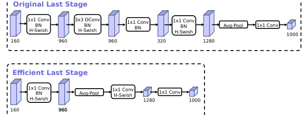
Figure 5. Comparison of original last stage and efficient last stage. This more efficient last stage is able to drop three expensive layers at the end of the network at no loss of accuracy.
图 5:原来的最后一段与高效最后一段的比较。更高效的最后一段能够去掉网络末尾的三个昂贵层,同时不损失精度。
Another expensive layer is the initial set of filters. Current mobile models tend to use 32 filters in a full 3x3 convolution to build initial filter banks for edge detection. Often these filters are mirror images of each other. We experimented with reducing the number of filters and using different nonlinearities to try and reduce redundancy. We settled on using the hard swish nonlinearity for this layer as it performed as well as other nonlinearities tested. We were able to reduce the number of filters to 16 while maintaining the same accuracy as 32 filters using either ReLU or swish. This saves an additional 2 milliseconds and 10 million MAdds.
另一处昂贵的层是最初的一组滤波器。当前的移动模型往往在完整的 3x3 卷积中使用 32 个滤波器,以建立用于边缘检测的初始滤波器组。这些滤波器常常互为镜像。我们尝试减少滤波器数量并换用不同非线性,以降低冗余。最终在这一层采用 hard swish 非线性,因为它与所测试的其他非线性表现相当。我们把滤波器数量减到 16,精度仍能达到使用 ReLU 或 swish 时 32 个滤波器的水平。这额外节省了 2 毫秒和 1000 万次乘加。
5.2. Nonlinearities
In [36, 13, 16] a nonlinearity called swish was introduced that when used as a drop-in replacement for ReLU, that significantly improves the accuracy of neural networks. The nonlinearity is defined as
[36, 13, 16] 引入了一种称为 swish 的非线性,当它作为 ReLU 的直接替换使用时,能显著提高神经网络的精度。该非线性定义为
While this nonlinearity improves accuracy, it comes with non-zero cost in embedded environments as the sigmoid function is much more expensive to compute on mobile devices. We deal with this problem in two ways.
虽然这种非线性能提高精度,但在嵌入式环境中并非没有代价,因为 sigmoid 函数在移动设备上计算要昂贵得多。我们从两个方面处理这一问题。
- We replace sigmoid function with its piece-wise linear hard analog: similar to [11, 44]. The minor difference is we use ReLU6 rather than a custom clipping constant. Similarly, the hard version of swish becomes
- 我们把 sigmoid 函数换成它的分段线性硬近似:,这与 [11, 44] 类似。细微差别是我们使用 ReLU6,而不是自定义的截断常数。类似地,swish 的硬版本变为
A similar version of hard-swish was also recently proposed in [2]. The comparison of the soft and hard version of sigmoid and swish nonlinearities is shown in figure 6. Our choice of constants was motivated by simplicity and being a good match to the original smooth version. In our experiments, we found hard-version of all these functions to have no discernible difference in accuracy, but multiple advantages from a deployment perspective. First, optimized implementations of ReLU6 are available on virtually all software and hardware frameworks. Second, in quantized mode, it eliminates potential numerical precision loss caused by different implementations of the approximate sigmoid. Finally, in practice, h-swish can be implemented as a piece-wise function to reduce the number of memory accesses driving the latency cost down substantially.
一种相近的 hard-swish 最近也在 [2] 中被提出。sigmoid 与 swish 非线性的软、硬版本比较见图 6。我们选择这些常数,既是为了简单,也是为了与原来的平滑版本良好吻合。实验中我们发现,这些函数的硬版本在精度上没有可察觉的差异,但从部署角度看有多项好处。第一,几乎所有软件和硬件框架上都有优化过的 ReLU6 实现。第二,在量化模式下,它消除了由近似 sigmoid 的不同实现可能带来的数值精度损失。最后,在实践中,h-swish 可以实现为分段函数,以减少内存访问次数,从而大幅降低延迟代价。
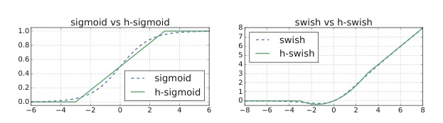
Figure 6. Sigmoid and swish nonlinearities and ther "hard" counterparts.
图 6:Sigmoid 与 swish 非线性及其“硬”对应形式。
- The cost of applying nonlinearity decreases as we go deeper into the network, since each layer activation memory typically halves every time the resolution drops. Incidentally, we find that most of the benefits swish are realized by using them only in the deeper layers. Thus in our architectures we only use h-swish at the second half of the model. We refer to the tables 1 and 2 for the precise layout.
- 施加非线性的代价会随着进入网络更深而下降,因为每当分辨率下降,每层激活所占内存通常减半。碰巧的是,我们发现 swish 的大部分好处只需用在更深的层就能获得。因此在我们的结构中,只在模型的后半段使用 h-swish。精确布局见表 1 和表 2。
Even with these optimizations, h-swish still introduces some latency cost. However as we demonstrate in section 6 the net effect on accuracy and latency is positive with no optimizations and substantial when using an optimized implementation based on a piece-wise function.
即便有这些优化,h-swish 仍会引入一些延迟代价。不过正如我们在第 6 节所展示的,即使不加优化,它对精度和延迟的净效果也是正面的;若采用基于分段函数的优化实现,收益则相当可观。
5.3. Large squeeze-and-excite
In [43], the size of the squeeze-and-excite bottleneck was relative the size of the convolutional bottleneck. Instead, we replace them all to fixed to be 1/4 of the number of channels in expansion layer. We find that doing so increases the accuracy, at the modest increase of number of parameters, and no discernible latency cost.
在 [43] 中,squeeze-and-excite 瓶颈的规模是相对于卷积瓶颈规模的。我们改为把它们全部固定为扩展层通道数的 1/4。我们发现这样做能提高精度,参数量只略有增加,且没有可察觉的延迟代价。
5.4. MobileNetV3 Definitions
MobileNetV3 is defined as two models: MobileNetV3-Large and MobileNetV3-Small. These models are targeted at high and low resource use cases respectively. The models are created through applying platform-aware NAS and NetAdapt for network search and incorporating the network improvements defined in this section. See table 1 and 2 for full specification of our networks.
MobileNetV3 定义为两个模型:MobileNetV3-Large 和 MobileNetV3-Small。它们分别面向高资源和低资源的使用场景。模型通过面向平台的 NAS 与 NetAdapt 进行网络搜索,并纳入本节定义的网络改进而得到。网络的完整规格见表 1 和表 2。
- Experiments
We present experimental results to demonstrate the effectiveness of the new MobileNetV3 models. We report results on classification, detection and segmentation. We also report various ablation studies to shed light on the effects of various design decisions.
我们给出实验结果,以展示新的 MobileNetV3 模型的效果。我们报告分类、检测和分割上的结果,并给出多项消融研究,以说明各种设计决策的影响。
6.1. Classification
As has become standard, we use ImageNet[38] for all our classification experiments and compare accuracy versus various measures of resource usage such as latency and multiply adds (MAdds).
按照现已通行的做法,我们的所有分类实验都使用 ImageNet[38],并比较精度与延迟、乘加次数(MAdds)等各种资源用量度量。
| Input | Operator | exp size | #out | SE | NL | |
|---|---|---|---|---|---|---|
| conv2d | - | 16 | - | HS | 2 | |
| bneck, 3x3 | 16 | 16 | - | RE | 1 | |
| bneck, 3x3 | 64 | 24 | - | RE | 2 | |
| bneck, 3x3 | 72 | 24 | - | RE | 1 | |
| bneck, 5x5 | 72 | 40 | ✓ | RE | 2 | |
| bneck, 5x5 | 120 | 40 | ✓ | RE | 1 | |
| bneck, 5x5 | 120 | 40 | ✓ | RE | 1 | |
| bneck, 3x3 | 240 | 80 | - | HS | 2 | |
| bneck, 3x3 | 200 | 80 | - | HS | 1 | |
| bneck, 3x3 | 184 | 80 | - | HS | 1 | |
| bneck, 3x3 | 184 | 80 | - | HS | 1 | |
| bneck, 3x3 | 480 | 112 | ✓ | HS | 1 | |
| bneck, 3x3 | 672 | 112 | ✓ | HS | 1 | |
| bneck, 5x5 | 672 | 160 | ✓ | HS | 2 | |
| bneck, 5x5 | 960 | 160 | ✓ | HS | 1 | |
| bneck, 5x5 | 960 | 160 | ✓ | HS | 1 | |
| conv2d, 1x1 | - | 960 | - | HS | 1 | |
| pool, 7x7 | - | - | - | - | 1 | |
| conv2d 1x1, NBN | - | 1280 | - | HS | 1 | |
| conv2d 1x1, NBN | - | - | - | 1 |
Table 1. Specification for MobileNetV3-Large. SE denotes whether there is a Squeeze-And-Excite in that block. NL denotes the type of nonlinearity used. Here, HS denotes h-swish and RE denotes ReLU. NBN denotes no batch normalization. denotes stride.
| 输入 | 算子 | 扩展规模 | 输出通道 | SE | NL | |
|---|---|---|---|---|---|---|
| conv2d | - | 16 | - | HS | 2 | |
| bneck, 3x3 | 16 | 16 | - | RE | 1 | |
| bneck, 3x3 | 64 | 24 | - | RE | 2 | |
| bneck, 3x3 | 72 | 24 | - | RE | 1 | |
| bneck, 5x5 | 72 | 40 | ✓ | RE | 2 | |
| bneck, 5x5 | 120 | 40 | ✓ | RE | 1 | |
| bneck, 5x5 | 120 | 40 | ✓ | RE | 1 | |
| bneck, 3x3 | 240 | 80 | - | HS | 2 | |
| bneck, 3x3 | 200 | 80 | - | HS | 1 | |
| bneck, 3x3 | 184 | 80 | - | HS | 1 | |
| bneck, 3x3 | 184 | 80 | - | HS | 1 | |
| bneck, 3x3 | 480 | 112 | ✓ | HS | 1 | |
| bneck, 3x3 | 672 | 112 | ✓ | HS | 1 | |
| bneck, 5x5 | 672 | 160 | ✓ | HS | 2 | |
| bneck, 5x5 | 960 | 160 | ✓ | HS | 1 | |
| bneck, 5x5 | 960 | 160 | ✓ | HS | 1 | |
| conv2d, 1x1 | - | 960 | - | HS | 1 | |
| pool, 7x7 | - | - | - | - | 1 | |
| conv2d 1x1, NBN | - | 1280 | - | HS | 1 | |
| conv2d 1x1, NBN | - | - | - | 1 |
表 1:MobileNetV3-Large 的规格。SE 表示该块中是否有 Squeeze-And-Excite。NL 表示所用非线性的类型,其中 HS 表示 h-swish,RE 表示 ReLU。NBN 表示没有批归一化。 表示步幅。
| Input | Operator | exp size | #out | SE | NL | |
|---|---|---|---|---|---|---|
| conv2d, 3x3 | - | 16 | - | HS | 2 | |
| bneck, 3x3 | 16 | 16 | ✓ | RE | 2 | |
| bneck, 3x3 | 72 | 24 | - | RE | 2 | |
| bneck, 3x3 | 88 | 24 | - | RE | 1 | |
| bneck, 5x5 | 96 | 40 | ✓ | HS | 2 | |
| bneck, 5x5 | 240 | 40 | ✓ | HS | 1 | |
| bneck, 5x5 | 240 | 40 | ✓ | HS | 1 | |
| bneck, 5x5 | 120 | 48 | ✓ | HS | 1 | |
| bneck, 5x5 | 144 | 48 | ✓ | HS | 1 | |
| bneck, 5x5 | 288 | 96 | ✓ | HS | 2 | |
| bneck, 5x5 | 576 | 96 | ✓ | HS | 1 | |
| bneck, 5x5 | 576 | 96 | ✓ | HS | 1 | |
| conv2d, 1x1 | - | 576 | ✓ | HS | 1 | |
| pool, 7x7 | - | - | - | - | 1 | |
| conv2d 1x1, NBN | - | 1280 | - | HS | 1 | |
| conv2d 1x1, NBN | - | - | - | 1 |
Table 2. Specification for MobileNetV3-Small. See table 1 for notation.
| 输入 | 算子 | 扩展规模 | 输出通道 | SE | NL | |
|---|---|---|---|---|---|---|
| conv2d, 3x3 | - | 16 | - | HS | 2 | |
| bneck, 3x3 | 16 | 16 | ✓ | RE | 2 | |
| bneck, 3x3 | 72 | 24 | - | RE | 2 | |
| bneck, 3x3 | 88 | 24 | - | RE | 1 | |
| bneck, 5x5 | 96 | 40 | ✓ | HS | 2 | |
| bneck, 5x5 | 240 | 40 | ✓ | HS | 1 | |
| bneck, 5x5 | 240 | 40 | ✓ | HS | 1 | |
| bneck, 5x5 | 120 | 48 | ✓ | HS | 1 | |
| bneck, 5x5 | 144 | 48 | ✓ | HS | 1 | |
| bneck, 5x5 | 288 | 96 | ✓ | HS | 2 | |
| bneck, 5x5 | 576 | 96 | ✓ | HS | 1 | |
| bneck, 5x5 | 576 | 96 | ✓ | HS | 1 | |
| conv2d, 1x1 | - | 576 | ✓ | HS | 1 | |
| pool, 7x7 | - | - | - | - | 1 | |
| conv2d 1x1, NBN | - | 1280 | - | HS | 1 | |
| conv2d 1x1, NBN | - | - | - | 1 |
表 2:MobileNetV3-Small 的规格。记号见表 1。
6.1.1 Training setup
We train our models using synchronous training setup on 4x4 TPU Pod [24] using standard tensorflow RMSPropOptimizer with 0.9 momentum. We use the initial learning rate of 0.1, with batch size 4096 (128 images per chip), and learning rate decay rate of 0.01 every 3 epochs. We use dropout of 0.8, and l2 weight decay 1e-5 and the same image preprocessing as Inception [42]. Finally we use exponential moving average with decay 0.9999. All our convolutional layers use batch-normalization layers with average decay of 0.99.
我们在 4x4 TPU Pod [24] 上采用同步训练设置,使用标准的 tensorflow RMSPropOptimizer,动量为 0.9。初始学习率为 0.1,batch 大小为 4096(每块芯片 128 张图),学习率每 3 个 epoch 按 0.01 的比率衰减。我们使用 0.8 的 dropout、1e-5 的 l2 权重衰减,以及与 Inception [42] 相同的图像预处理。最后使用衰减为 0.9999 的指数滑动平均。所有卷积层都使用平均衰减为 0.99 的批归一化层。
6.1.2 Measurement setup
To measure latencies we use standard Google Pixel phones and run all networks through the standard TFLite Benchmark Tool. We use single-threaded large core in all our measurements. We don't report multi-core inference time, since we find this setup not very practical for mobile applications. We contributed an atomic h-swish operator to tensorflow lite, and it is now default in the latest version. We show the impact of optimized h-swish on figure 9.
为测量延迟,我们使用标准的 Google Pixel 手机,并通过标准的 TFLite Benchmark Tool 运行所有网络。所有测量都使用单线程大核。我们不报告多核推理时间,因为发现这种设置对移动应用并不十分实用。我们向 TensorFlow Lite 贡献了一个原子的 h-swish 算子,它现已成为最新版本中的默认实现。优化后的 h-swish 的影响见图 9。
6.2. Results
As can be seen on figure 1 our models outperform the current state of the art such as MnasNet [43], ProxylessNas [5] and MobileNetV2 [39]. We report the floating point performance on different Pixel phones in the table 3. We include quantization results in table 4.
如图 1 所示,我们的模型优于当时的最优方法,例如 MnasNet [43]、ProxylessNas [5] 和 MobileNetV2 [39]。我们在表 3 中报告不同 Pixel 手机上的浮点性能,量化结果见表 4。
| Network | Top-1 | MAdds | Params | P-1 | P-2 | P-3 |
|---|---|---|---|---|---|---|
| V3-Large 1.0 | 75.2 | 219 | 5.4M | 51 | 61 | 44 |
| V3-Large 0.75 | 73.3 | 155 | 4.0M | 39 | 46 | 40 |
| MnasNet-A1 | 75.2 | 315 | 3.9M | 71 | 86 | 61 |
| Proxyless[5] | 74.6 | 320 | 4.0M | 72 | 84 | 60 |
| V2 1.0 | 72.0 | 300 | 3.4M | 64 | 76 | 56 |
| V3-Small 1.0 | 67.4 | 66 | 2.9M | 15.8 | 19.4 | 14.4 |
| V3-Small 0.75 | 65.4 | 44 | 2.4M | 12.8 | 15.6 | 11.7 |
| Mnas-small [43] | 64.9 | 65.1 | 1.9M | 20.3 | 24.2 | 17.2 |
| V2 0.35 | 60.8 | 59.2 | 1.6M | 16.6 | 19.6 | 13.9 |
Table 3. Floating point performance on the Pixel family of phones (P- denotes a Pixel- phone). All latencies are in ms and are measured using a single large core with a batch size of one. Top-1 accuracy is on ImageNet.
| 网络 | Top-1 | MAdds | 参数量 | P-1 | P-2 | P-3 |
|---|---|---|---|---|---|---|
| V3-Large 1.0 | 75.2 | 219 | 5.4M | 51 | 61 | 44 |
| V3-Large 0.75 | 73.3 | 155 | 4.0M | 39 | 46 | 40 |
| MnasNet-A1 | 75.2 | 315 | 3.9M | 71 | 86 | 61 |
| Proxyless[5] | 74.6 | 320 | 4.0M | 72 | 84 | 60 |
| V2 1.0 | 72.0 | 300 | 3.4M | 64 | 76 | 56 |
| V3-Small 1.0 | 67.4 | 66 | 2.9M | 15.8 | 19.4 | 14.4 |
| V3-Small 0.75 | 65.4 | 44 | 2.4M | 12.8 | 15.6 | 11.7 |
| Mnas-small [43] | 64.9 | 65.1 | 1.9M | 20.3 | 24.2 | 17.2 |
| V2 0.35 | 60.8 | 59.2 | 1.6M | 16.6 | 19.6 | 13.9 |
表 3:Pixel 系列手机上的浮点性能(P- 表示 Pixel- 手机)。所有延迟以毫秒计,并在单颗大核、batch 大小为 1 的条件下测得。Top-1 精度针对 ImageNet。
| Network | Top-1 | P-1 | P-2 | P-3 |
|---|---|---|---|---|
| V3-Large 1.0 | 73.8 | 44 | 42.5 | 31.7 |
| V2 1.0 | 70.9 | 52 | 48.3 | 37.0 |
| V3-Small | 64.9 | 15.5 | 14.9 | 10.7 |
| V2 0.35 | 57.2 | 16.7 | 15.6 | 11.9 |
Table 4. Quantized performance. All latencies are in ms. The inference latency is measured using a single large core on the respective Pixel 1/2/3 device.
| 网络 | Top-1 | P-1 | P-2 | P-3 |
|---|---|---|---|---|
| V3-Large 1.0 | 73.8 | 44 | 42.5 | 31.7 |
| V2 1.0 | 70.9 | 52 | 48.3 | 37.0 |
| V3-Small | 64.9 | 15.5 | 14.9 | 10.7 |
| V2 0.35 | 57.2 | 16.7 | 15.6 | 11.9 |
表 4:量化性能。所有延迟以毫秒计。推理延迟在相应的 Pixel 1/2/3 设备上使用单颗大核测得。
In figure 7 we show the MobileNetV3 performance trade-offs as a function of multiplier and resolution. Note how MobileNetV3-Small outperforms the MobileNetV3-Large with multiplier scaled to match the performance by nearly 3%. On the other hand, resolution provides an even better trade-offs than multiplier. However, it should be noted that resolution is often determined by the problem (e.g. segmentation and detection problem generally require higher resolution), and thus can't always be used as a tunable parameter.
图 7 展示了 MobileNetV3 作为乘数和分辨率函数的性能权衡。请注意,把 MobileNetV3-Large 的乘数缩放到相近性能时,MobileNetV3-Small 仍高出近 3 个百分点。另一方面,分辨率给出的权衡甚至比乘数更好。不过应当指出,分辨率常常由问题本身决定(例如分割和检测通常需要更高分辨率),因此并不总能当作可调参数来用。
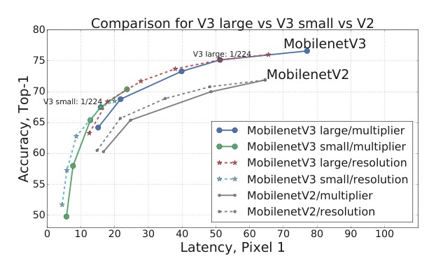
Figure 7. Performance of MobileNetV3 as a function of different multipliers and resolutions. In our experiments we have used multipliers 0.35, 0.5, 0.75, 1.0 and 1.25, with a fixed resolution of 224, and resolutions 96, 128, 160, 192, 224 and 256 with a fixed depth multiplier of 1.0. Best viewed in color. Top-1 accuracy is on ImageNet and latency is in ms.
图 7:MobileNetV3 在不同乘数和分辨率下的性能。实验中我们使用乘数 0.35、0.5、0.75、1.0 和 1.25,并固定分辨率为 224;以及分辨率 96、128、160、192、224 和 256,并固定深度乘数为 1.0。建议彩色查看。Top-1 精度针对 ImageNet,延迟以毫秒计。
6.2.1 Ablation study
Impact of non-linearities. In table 5 we study the choice of where to insert h-swish nonlinearities as well as the improvements of using an optimized implementation over a naive implementation. It can be seen that using an optimized implementation of h-swish saves 6ms (more than 10% of the runtime). Optimized h-swish only adds an additional 1ms compared to traditional ReLU.
非线性的影响。在表 5 中,我们研究把 h-swish 非线性插在何处,以及优化实现相对朴素实现的改进。可以看到,使用优化后的 h-swish 实现能节省 6 毫秒(超过运行时间的 10%)。与传统 ReLU 相比,优化后的 h-swish 只额外增加 1 毫秒。
| Top-1 | P-1 | P-1 (no-opt) | |
|---|---|---|---|
| V3-Large 1.0 | 75.2 | 51.4 | 57.5 |
| ReLU | 74.5 (-.7%) | 50.5 (-1%) | 50.5 |
| h-swish @16 | 75.4 (+.2%) | 53.5 (+4%) | 68.9 |
| h-swish @112 | 75.0 (-.3%) | 51 (-0.5%) | 54.4 |
Table 5. Effect of non-linearities on MobileNetV3-Large. In h-swish @, denotes the number of channels, in the first layer that has h-swish enabled. The third column shows the runtime without optimized h-swish. Top-1 accuracy is on ImageNet and latency is in ms.
| Top-1 | P-1 | P-1(未优化) | |
|---|---|---|---|
| V3-Large 1.0 | 75.2 | 51.4 | 57.5 |
| ReLU | 74.5(-0.7%) | 50.5(-1%) | 50.5 |
| h-swish @16 | 75.4(+0.2%) | 53.5(+4%) | 68.9 |
| h-swish @112 | 75.0(-0.3%) | 51(-0.5%) | 54.4 |
表 5:非线性对 MobileNetV3-Large 的影响。在 h-swish @ 中, 表示第一个启用 h-swish 的层的通道数。第三列给出未优化 h-swish 时的运行时间。Top-1 精度针对 ImageNet,延迟以毫秒计。
Figure 8 shows the efficient frontier based on nonlinearity choices and network width. MobileNetV3 uses h-swish in the middle of the network and clearly dominates ReLU. It is interesting to note that adding h-swish to the entire network is slightly better than the interpolated frontier of widening the network.
图 8 给出了基于非线性选择和网络宽度的高效前沿。MobileNetV3 在网络中部使用 h-swish,并明显优于 ReLU。有意思的是,把 h-swish 加到整个网络上,略好于加宽网络所得到的插值前沿。
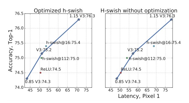
Figure 8. Impact of h-swish vs ReLU on latency for optimized and non-optimized h-swish. The curve shows a frontier of using depth multiplier. Note that placing h-swish at all layers with 80 channels or more (V3) provides the best trade-offs for both optimized h-swish and non-optimized h-swish. Top-1 accuracy is on ImageNet and latency is in ms.
图 8:优化与未优化的 h-swish 相对 ReLU 对延迟的影响。曲线给出使用深度乘数时的前沿。请注意,在所有通道数不少于 80 的层上放置 h-swish(即 V3)无论对优化还是未优化的 h-swish,都给出了最好的权衡。Top-1 精度针对 ImageNet,延迟以毫秒计。
Impact of other components. In figure 9 we show how introduction of different components moved along the latency/accuracy curve.
其他组件的影响。图 9 展示了引入不同组件后,模型如何沿着延迟/精度曲线移动。
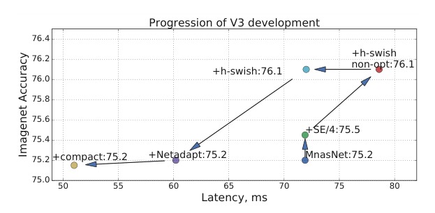
Figure 9. Impact of individual components in the development of MobileNetV3. Progress is measured by moving up and to the left.
图 9:MobileNetV3 开发过程中各个组件的影响。进展以向上、向左移动来衡量。
6.3. Detection
We use MobileNetV3 as a drop-in replacement for the backbone feature extractor in SSDLite [39] and compare with other backbone networks on COCO dataset [26].
我们把 MobileNetV3 作为 SSDLite [39] 中骨干特征提取器的即插即用替换,并在 COCO 数据集 [26] 上与其他骨干网络进行比较。
Following MobileNetV2 [39], we attach the first layer of SSDLite to the last feature extractor layer that has an output stride of 16, and attach the second layer of SSDLite to the last feature extractor layer that has an output stride of 32. Following the detection literature, we refer to these two feature extractor layers as C4 and C5, respectively. For MobileNetV3-Large, C4 is the expansion layer of the 13-th bottleneck block. For MobileNetV3-Small, C4 is the expansion layer of the 9-th bottleneck block. For both networks, C5 is the layer immediately before pooling.
沿用 MobileNetV2 [39],我们把 SSDLite 的第一层接到输出步幅为 16 的最后一个特征提取层,把第二层接到输出步幅为 32 的最后一个特征提取层。按检测文献的习惯,这两个特征提取层分别称为 C4 和 C5。对 MobileNetV3-Large,C4 是第 13 个瓶颈块的扩展层;对 MobileNetV3-Small,C4 是第 9 个瓶颈块的扩展层。对两个网络,C5 都是紧挨池化之前的那一层。
We additionally reduce the channel counts of all feature layers between C4 and C5 by 2. This is because the last few layers of MobileNetV3 are tuned to output 1000 classes, which may be redundant when transferred to COCO with 90 classes. The results on COCO test set are given in Tab. 6. With the channel reduction, MobileNetV3-Large is 27% faster than MobileNetV2 with near identical mAP. MobileNetV3-Small with channel reduction is also 2.4 and 0.5 mAP higher than MobileNetV2 and MnasNet while being 35% faster. For both MobileNetV3 models the channel reduction trick contributes to approximately 15% latency reduction with no mAP loss, suggesting that ImageNet classification and COCO object detection may prefer different feature extractor shapes.
我们还把 C4 与 C5 之间所有特征层的通道数减半。这是因为 MobileNetV3 的最后几层是为输出 1000 类而调的,迁移到只有 90 类的 COCO 上可能有冗余。COCO 测试集上的结果见表 6。经过通道缩减后,MobileNetV3-Large 比 MobileNetV2 快 27%,mAP 几乎相同。经过通道缩减的 MobileNetV3-Small 也分别比 MobileNetV2 和 MnasNet 高 2.4 和 0.5 个 mAP,同时快 35%。对两个 MobileNetV3 模型,这一通道缩减技巧都贡献了约 15% 的延迟下降,且不损失 mAP,说明 ImageNet 分类和 COCO 目标检测可能偏好不同的特征提取器形状。
| Backbone | mAP | Latency (ms) | Params (M) | MAdds (B) |
|---|---|---|---|---|
| V1 | 22.2 | 228 | 5.1 | 1.3 |
| V2 | 22.1 | 162 | 4.3 | 0.80 |
| MnasNet | 23.0 | 174 | 4.88 | 0.84 |
| V3 | 22.0 | 137 | 4.97 | 0.62 |
| V3 | 22.0 | 119 | 3.22 | 0.51 |
| V2 0.35 | 13.7 | 66 | 0.93 | 0.16 |
| V2 0.5 | 16.6 | 79 | 1.54 | 0.27 |
| MnasNet 0.35 | 15.6 | 68 | 1.02 | 0.18 |
| MnasNet 0.5 | 18.5 | 85 | 1.68 | 0.29 |
| V3-Small | 16.0 | 52 | 2.49 | 0.21 |
| V3-Small | 16.1 | 43 | 1.77 | 0.16 |
Table 6. Object detection results of SSDLite with different backbones on COCO test set. : Channels in the blocks between and are reduced by a factor of 2.
| 骨干 | mAP | 延迟(ms) | 参数量(M) | MAdds(B) |
|---|---|---|---|---|
| V1 | 22.2 | 228 | 5.1 | 1.3 |
| V2 | 22.1 | 162 | 4.3 | 0.80 |
| MnasNet | 23.0 | 174 | 4.88 | 0.84 |
| V3 | 22.0 | 137 | 4.97 | 0.62 |
| V3 | 22.0 | 119 | 3.22 | 0.51 |
| V2 0.35 | 13.7 | 66 | 0.93 | 0.16 |
| V2 0.5 | 16.6 | 79 | 1.54 | 0.27 |
| MnasNet 0.35 | 15.6 | 68 | 1.02 | 0.18 |
| MnasNet 0.5 | 18.5 | 85 | 1.68 | 0.29 |
| V3-Small | 16.0 | 52 | 2.49 | 0.21 |
| V3-Small | 16.1 | 43 | 1.77 | 0.16 |
表 6:不同骨干的 SSDLite 在 COCO 测试集上的目标检测结果。:将 与 之间各块的通道数减半。
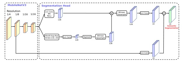
Figure 10. Building on MobileNetV3, the proposed segmentation head, Lite R-ASPP, delivers fast semantic segmentation results while mixing features from multiple resolutions.
图 10:以 MobileNetV3 为基础,所提出的分割头 Lite R-ASPP 在混合多分辨率特征的同时,给出快速的语义分割结果。
6.4. Semantic Segmentation
In this subsection, we employ MobileNetV2 [39] and the proposed MobileNetV3 as network backbones for the task of mobile semantic segmentation. Additionally, we compare two segmentation heads. The first one, referred to as R-ASPP, was proposed in [39]. R-ASPP is a reduced design of the Atrous Spatial Pyramid Pooling module [7, 8, 9], which adopts only two branches consisting of a convolution and a global-average pooling operation [29, 50]. In this work, we propose another light-weight segmentation head, referred to as Lite R-ASPP (or LR-ASPP), as shown in Fig. 10. Lite R-ASPP, improving over R-ASPP, deploys the global-average pooling in a fashion similar to the Squeeze-and-Excitation module [20], in which we employ a large pooling kernel with a large stride (to save some computation) and only one convolution in the module. We apply atrous convolution [18, 40, 33, 6] to the last block of MobileNetV3 to extract denser features, and further add a skip connection [30] from low-level features to capture more detailed information.
本小节将 MobileNetV2 [39] 和所提出的 MobileNetV3 用作移动语义分割任务的网络骨干,并比较两种分割头。第一种称为 R-ASPP,由 [39] 提出。R-ASPP 是空洞空间金字塔池化模块 [7, 8, 9] 的简化设计,只采用两个分支,分别是 卷积和全局平均池化 [29, 50]。本文提出另一种轻量分割头,称为 Lite R-ASPP(或 LR-ASPP),如图 10 所示。Lite R-ASPP 在 R-ASPP 之上加以改进,以类似 Squeeze-and-Excitation 模块 [20] 的方式布置全局平均池化:采用大的池化核和大步幅(以节省一些计算),并且模块中只有一次 卷积。我们对 MobileNetV3 的最后一个块使用空洞卷积 [18, 40, 33, 6] 以提取更密的特征,并进一步加入来自低层特征的跳连 [30],以捕获更细致的信息。
We conduct the experiments on the Cityscapes dataset [10] with metric mIOU [14], and only exploit the 'fine' annotations. We employ the same training protocol as [8, 39]. All our models are trained from scratch without pretraining on ImageNet [38], and are evaluated with a single-scale input. Similar to object detection, we observe that we could reduce the channels in the last block of network backbone by a factor of 2 without degrading the performance significantly. We think it is because the backbone is designed for 1000 classes ImageNet image classification [38] while there are only 19 classes on Cityscapes, implying there is some channel redundancy in the backbone.
我们在 Cityscapes 数据集 [10] 上以 mIOU [14] 为度量进行实验,并且只使用“精细”(fine)标注。训练协议与 [8, 39] 相同。所有模型都从零训练,不在 ImageNet [38] 上预训练,并使用单尺度输入评估。与目标检测类似,我们观察到可以把网络骨干最后一个块的通道数减半,而不显著降低性能。我们认为这是因为骨干是为 1000 类的 ImageNet 图像分类 [38] 设计的,而 Cityscapes 上只有 19 类,说明骨干中存在一些通道冗余。
We report our Cityscapes validation set results in Tab. 7. As shown in the table, we observe that (1) reducing the channels in the last block of network backbone by a factor of 2 significantly improves the speed while maintaining similar performances (row 1 vs. row 2, and row 5 vs. row 6), (2) the proposed segmentation head LR-ASPP is slightly faster than R-ASPP [39] while performance is improved (row 2 vs. row 3, and row 6 vs. row 7), (3) reducing the filters in the segmentation head from 256 to 128 improves the speed at the cost of slightly worse performance (row 3 vs. row 4, and row 7 vs. row 8), (4) when employing the same setting, MobileNetV3 model variants attain similar performance while being slightly faster than MobileNetV2 counterparts (row 1 vs. row 5, row 2 vs. row 6, row 3 vs. row 7, and row 4 vs. row 8), (5) MobileNetV3-Small attains similar performance as MobileNetV2-0.5 while being faster, and (6) MobileNetV3-Small is significantly better than MobileNetV2-0.35 while yielding similar speed.
我们在表 7 中报告 Cityscapes 验证集结果。如表所示,我们观察到:(1) 把网络骨干最后一个块的通道数减半,能显著提高速度,同时保持相近的性能(第 1 行对第 2 行,以及第 5 行对第 6 行);(2) 所提出的分割头 LR-ASPP 比 R-ASPP [39] 略快,同时性能有所提升(第 2 行对第 3 行,以及第 6 行对第 7 行);(3) 把分割头中的滤波器从 256 减到 128,能提高速度,代价是性能略差(第 3 行对第 4 行,以及第 7 行对第 8 行);(4) 在相同设置下,MobileNetV3 的各变体达到相近性能,同时比对应的 MobileNetV2 略快(第 1 行对第 5 行,第 2 行对第 6 行,第 3 行对第 7 行,以及第 4 行对第 8 行);(5) MobileNetV3-Small 达到与 MobileNetV2-0.5 相近的性能,同时更快;(6) MobileNetV3-Small 明显优于 MobileNetV2-0.35,同时速度相近。
| N | Backbone | RF2 | SH | F | mIOU | Params | MAdds | CPU (f) | CPU (h) |
|---|---|---|---|---|---|---|---|---|---|
| 1 | V2 | - | × | 256 | 72.84 | 2.11M | 21.29B | 3.90s | 1.02s |
| 2 | V2 | ✓ | × | 256 | 72.56 | 1.15M | 13.68B | 3.03s | 793ms |
| 3 | V2 | ✓ | ✓ | 256 | 72.97 | 1.02M | 12.83B | 2.98s | 786ms |
| 4 | V2 | ✓ | ✓ | 128 | 72.74 | 0.98M | 12.57B | 2.89s | 766ms |
| 5 | V3 | - | × | 256 | 72.64 | 3.60M | 18.43B | 3.55s | 906ms |
| 6 | V3 | ✓ | × | 256 | 71.91 | 1.76M | 11.24B | 2.60s | 668ms |
| 7 | V3 | ✓ | ✓ | 256 | 72.37 | 1.63M | 10.33B | 2.55s | 659ms |
| 8 | V3 | ✓ | ✓ | 128 | 72.36 | 1.51M | 9.74B | 2.47s | 657ms |
| 9 | V2 0.5 | ✓ | ✓ | 128 | 68.57 | 0.28M | 4.00B | 1.59s | 415ms |
| 10 | V2 0.35 | ✓ | ✓ | 128 | 66.83 | 0.16M | 2.54B | 1.27s | 354ms |
| 11 | V3-Small | ✓ | ✓ | 128 | 68.38 | 0.47M | 2.90B | 1.21s | 327ms |
Table 7. Semantic segmentation results on Cityscapes val set. RF2: Reduce the Filters in the last block by a factor of 2. V2 0.5 and V2 0.35 are MobileNetV2 with depth multiplier = 0.5 and 0.35, respectively. SH: Segmentation Head, where × employs the R-ASPP while ✓ employs the proposed LR-ASPP. F: Number of Filters used in the Segmentation Head. CPU (f): CPU time measured on a single large core of Pixel 3 (floating point) w.r.t. a full-resolution input (i.e., ). CPU (h): CPU time measured w.r.t. a half-resolution input (i.e., ). Row 8, and 11 are our MobileNetV3 segmentation candidates.
| N | 骨干 | RF2 | SH | F | mIOU | 参数量 | MAdds | CPU (f) | CPU (h) |
|---|---|---|---|---|---|---|---|---|---|
| 1 | V2 | - | × | 256 | 72.84 | 2.11M | 21.29B | 3.90s | 1.02s |
| 2 | V2 | ✓ | × | 256 | 72.56 | 1.15M | 13.68B | 3.03s | 793ms |
| 3 | V2 | ✓ | ✓ | 256 | 72.97 | 1.02M | 12.83B | 2.98s | 786ms |
| 4 | V2 | ✓ | ✓ | 128 | 72.74 | 0.98M | 12.57B | 2.89s | 766ms |
| 5 | V3 | - | × | 256 | 72.64 | 3.60M | 18.43B | 3.55s | 906ms |
| 6 | V3 | ✓ | × | 256 | 71.91 | 1.76M | 11.24B | 2.60s | 668ms |
| 7 | V3 | ✓ | ✓ | 256 | 72.37 | 1.63M | 10.33B | 2.55s | 659ms |
| 8 | V3 | ✓ | ✓ | 128 | 72.36 | 1.51M | 9.74B | 2.47s | 657ms |
| 9 | V2 0.5 | ✓ | ✓ | 128 | 68.57 | 0.28M | 4.00B | 1.59s | 415ms |
| 10 | V2 0.35 | ✓ | ✓ | 128 | 66.83 | 0.16M | 2.54B | 1.27s | 354ms |
| 11 | V3-Small | ✓ | ✓ | 128 | 68.38 | 0.47M | 2.90B | 1.21s | 327ms |
表 7:Cityscapes 验证集上的语义分割结果。RF2:把最后一个块中的滤波器数减半。V2 0.5 和 V2 0.35 分别是深度乘数为 0.5 和 0.35 的 MobileNetV2。SH:分割头,其中 × 表示使用 R-ASPP,✓ 表示使用所提出的 LR-ASPP。F:分割头中使用的滤波器数。CPU (f):在 Pixel 3 单颗大核上相对全分辨率输入(即 )测得的浮点 CPU 时间。CPU (h):相对半分辨率输入(即 )测得的 CPU 时间。第 8 行和第 11 行是我们的 MobileNetV3 分割候选。
Tab. 8 shows our Cityscapes test set results. Our segmentation models with MobileNetV3 as network backbone outperforms ESPNetv2 [32], CCC2 [34], and ESPNetv1 [32] by 6.4%, 10.6%, 12.3%, respectively while being faster in terms of MAdds. The performance drops slightly by 0.6% when not employing the atrous convolution to extract dense feature maps in the last block of MobileNetV3, but the speed is improved to 1.98B (for half-resolution inputs), which is 1.36, 1.59, and 2.27 times faster than ESPNetv2, CCC2, and ESPNetv1, respectively. Furthermore, our models with MobileNetV3-Small as network backbone still outperforms all of them by at least a healthy margin of 2.1%.
表 8 给出我们在 Cityscapes 测试集上的结果。以 MobileNetV3 为网络骨干的分割模型分别比 ESPNetv2 [32]、CCC2 [34] 和 ESPNetv1 [32] 高 6.4%、10.6%、12.3%,同时在 MAdds 上更快。若在 MobileNetV3 的最后一个块中不使用空洞卷积来提取稠密特征图,性能只略降 0.6%,但速度提升到 1.98B(相对半分辨率输入),分别比 ESPNetv2、CCC2 和 ESPNetv1 快 1.36、1.59 和 2.27 倍。此外,以 MobileNetV3-Small 为骨干的模型仍至少以 2.1 个百分点的可观优势超过上述所有方法。
| Backbone | OS | mIOU | MAdds (f) | MAdds (h) | CPU (f) | CPU (h) |
|---|---|---|---|---|---|---|
| V3 | 16 | 72.6 | 9.74B | 2.48B | 2.47s | 657ms |
| V3 | 32 | 72.0 | 7.74B | 1.98B | 2.06s | 534ms |
| V3-Small | 16 | 69.4 | 2.90B | 0.74B | 1.21s | 327ms |
| V3-Small | 32 | 68.3 | 2.06B | 0.53B | 1.03s | 275ms |
| ESPNetv2 [32] | - | 66.2 | - | 2.7B | - | - |
| CCC2 [34] | - | 62.0 | - | 3.15B | - | - |
| ESPNetv1 [31] | - | 60.3 | - | 4.5B | - | - |
Table 8. Semantic segmentation results on Cityscapes test set. OS: Output Stride, the ratio of input image spatial resolution to backbone output resolution. When OS = 16, atrous convolution is applied in the last block of backbone. When OS = 32, no atrous convolution is used. MAdds (f): Multiply-Adds measured w.r.t. a full-resolution input (i.e., ). MAdds (h): Multiply-Adds measured w.r.t. a half-resolution input (i.e., ). CPU (f): CPU time measured on a single large core of Pixel 3 (floating point) w.r.t. a full-resolution input (i.e., ). CPU (h): CPU time measured w.r.t. a half-resolution input (i.e., ). ESPNet [31, 32] and CCC2 [34] take half resolution inputs, while our models directly take full-resolution inputs.
| 骨干 | OS | mIOU | MAdds (f) | MAdds (h) | CPU (f) | CPU (h) |
|---|---|---|---|---|---|---|
| V3 | 16 | 72.6 | 9.74B | 2.48B | 2.47s | 657ms |
| V3 | 32 | 72.0 | 7.74B | 1.98B | 2.06s | 534ms |
| V3-Small | 16 | 69.4 | 2.90B | 0.74B | 1.21s | 327ms |
| V3-Small | 32 | 68.3 | 2.06B | 0.53B | 1.03s | 275ms |
| ESPNetv2 [32] | - | 66.2 | - | 2.7B | - | - |
| CCC2 [34] | - | 62.0 | - | 3.15B | - | - |
| ESPNetv1 [31] | - | 60.3 | - | 4.5B | - | - |
表 8:Cityscapes 测试集上的语义分割结果。OS:输出步幅,即输入图像空间分辨率与骨干输出分辨率之比。当 OS = 16 时,在骨干最后一个块中使用空洞卷积;当 OS = 32 时,不使用空洞卷积。MAdds (f):相对全分辨率输入(即 )测得的乘加次数。MAdds (h):相对半分辨率输入(即 )测得的乘加次数。CPU (f):在 Pixel 3 单颗大核上相对全分辨率输入(即 )测得的浮点 CPU 时间。CPU (h):相对半分辨率输入(即 )测得的 CPU 时间。ESPNet [31, 32] 和 CCC2 [34] 使用半分辨率输入,而我们的模型直接使用全分辨率输入。
- Conclusions and future work
In this paper we introduced MobileNetV3 Large and Small models demonstrating new state of the art in mobile classification, detection and segmentation. We have described our efforts to harness multiple network architecture search algorithms as well as advances in network design to deliver the next generation of mobile models. We have also shown how to adapt nonlinearities like swish and apply squeeze and excite in a quantization friendly and efficient manner introducing them into the mobile model domain as effective tools. We also introduced a new form of lightweight segmentation decoders called LR-ASPP. While it remains an open question of how best to blend automatic search techniques with human intuition, we are pleased to present these first positive results and will continue to refine methods as future work.
本文介绍了 MobileNetV3 Large 和 Small 模型,它们在移动端分类、检测和分割上展示了新的当时最优水平。我们描述了如何借助多种网络结构搜索算法以及网络设计上的进展,交出下一代移动模型。我们还展示了如何以利于量化和高效的方式改写 swish 这类非线性,并应用 squeeze-and-excite,从而把它们作为有效工具引入移动模型领域。我们还提出了一种新的轻量分割解码器,称为 LR-ASPP。如何最好地把自动搜索技术与人的直觉结合起来,仍然是一个开放问题;我们很高兴给出这些初步的正面结果,并将在未来工作中继续改进方法。
Acknowledgements
致谢
We would like to thank Andrey Zhmoginov, Dmitry Kalenichenko, Menglong Zhu, Jon Shlens, Xiao Zhang, Benoit Jacob, Alex Stark, Achille Brighton and Sergey Ioffe for helpful feedback and discussion.
我们感谢 Andrey Zhmoginov、Dmitry Kalenichenko、Menglong Zhu、Jon Shlens、Xiao Zhang、Benoit Jacob、Alex Stark、Achille Brighton 和 Sergey Ioffe 提供的有益反馈与讨论。
References
参考文献
[1] Martín Abadi, Ashish Agarwal, Paul Barham, Eugene Brevdo, Zhifeng Chen, Craig Citro, Greg S. Corrado, Andy Davis, Jeffrey Dean, Matthieu Devin, Sanjay Ghemawat, Ian Goodfellow, Andrew Harp, Geoffrey Irving, Michael Isard, Yangqing Jia, Rafal Jozefowicz, Lukasz Kaiser, Manjunath Kudlur, Josh Levenberg, Dan Man´e, Rajat Monga, Sherry Moore, Derek Murray, Chris Olah, Mike Schuster, Jonathon Shlens, Benoit Steiner, Ilya Sutskever, Kunal Talwar, Paul Tucker, Vincent Vanhoucke, Vijay Vasudevan, Fernanda Vi´egas, Oriol Vinyals, Pete Warden, Martin Wattenberg, Martin Wicke, Yuan Yu, and Xiaoqiang Zheng. Tensor- Flow: Large-scale machine learning on heterogeneous systems, 2015. Software available from tensorflow.org. 1
[2] R. Avenash and P. Vishawanth. Semantic segmentation of satellite images using a modified cnn with hard-swish activation function. In VISIGRAPP, 2019. 2, 4
[3] Bowen Baker, Otkrist Gupta, Nikhil Naik, and Ramesh Raskar. Designing neural network architectures using reinforcement learning. CoRR, abs/1611.02167, 2016. 2
[4] Cristian Buciluˇa, Rich Caruana, and Alexandru Niculescu- Mizil. Model compression. In Proceedings of the 12th ACM SIGKDD International Conference on Knowledge Discovery and Data Mining, KDD ’06, pages 535–541, New York, NY, USA, 2006. ACM. 2
[5] Han Cai, Ligeng Zhu, and Song Han. Proxylessnas: Direct neural architecture search on target task and hardware. CoRR, abs/1812.00332, 2018. 2, 3, 6
[6] Liang-Chieh Chen, George Papandreou, Iasonas Kokkinos, Kevin Murphy, and Alan L Yuille. Semantic image segmentation with deep convolutional nets and fully connected crfs. In ICLR, 2015. 7
[7] Liang-Chieh Chen, George Papandreou, Iasonas Kokkinos, Kevin Murphy, and Alan L Yuille. Deeplab: Semantic image segmentation with deep convolutional nets, atrous convolution, and fully connected crfs. TPAMI, 2017. 7
[8] Liang-Chieh Chen, George Papandreou, Florian Schroff, and Hartwig Adam. Rethinking atrous convolution for semantic image segmentation. CoRR, abs/1706.05587, 2017. 7, 8
[9] Liang-Chieh Chen, Yukun Zhu, George Papandreou, Florian Schroff, and Hartwig Adam. Encoder-decoder with atrous separable convolution for semantic image segmentation. In ECCV, 2018. 7
[10] Marius Cordts, Mohamed Omran, Sebastian Ramos, Timo Rehfeld, Markus Enzweiler, Rodrigo Benenson, Uwe Franke, Stefan Roth, and Bernt Schiele. The cityscapes dataset for semantic urban scene understanding. In CVPR, 2016. 8
[11] Matthieu Courbariaux, Yoshua Bengio, and Jean-Pierre David. Binaryconnect: Training deep neural networks with binary weights during propagations. CoRR, abs/1511.00363, 2015. 2, 4
[12] Xiaoliang Dai, Peizhao Zhang, Bichen Wu, Hongxu Yin, Fei Sun, Yanghan Wang, Marat Dukhan, Yunqing Hu, Yiming Wu, Yangqing Jia, Peter Vajda, Matt Uyttendaele, and Niraj K. Jha. Chamnet: Towards efficient network de- sign through platform-aware model adaptation. CoRR, abs/1812.08934, 2018. 2
[13] Stefan Elfwing, Eiji Uchibe, and Kenji Doya. Sigmoidweighted linear units for neural network function approximation in reinforcement learning. CoRR, abs/1702.03118, 2017. 2, 4
[14] Mark Everingham, S. M. Ali Eslami, Luc Van Gool, Christo- pher K. I. Williams, John Winn, and Andrew Zisserma. The pascal visual object classes challenge a retrospective. IJCV, 2014. 8
[15] Yihui He and Song Han. AMC: automated deep compres- sion and acceleration with reinforcement learning. In ECCV, 2018. 2
[16] Dan Hendrycks and Kevin Gimpel. Bridging nonlinearities and stochastic regularizers with gaussian error linear units. CoRR, abs/1606.08415, 2016. 2, 4
[17] Geoffrey Hinton, Oriol Vinyals, and Jeffrey Dean. Distilling the knowledge in a neural network. In NIPS Deep Learning and Representation Learning Workshop, 2015. 2
[18] Matthias Holschneider, Richard Kronland-Martinet, Jean Morlet, and Ph Tchamitchian. A real-time algorithm for signal analysis with the help of the wavelet transform. In Wavelets: Time-Frequency Methods and Phase Space, pages 289–297. Springer Berlin Heidelberg, 1989. 7
[19] Andrew G. Howard, Menglong Zhu, Bo Chen, Dmitry Kalenichenko, Weijun Wang, Tobias Weyand, Marco Andreetto, and Hartwig Adam. Mobilenets: Efficient convolutional neural networks for mobile vision applications. CoRR, abs/1704.04861, 2017. 2
[20] J. Hu, L. Shen, and G. Sun. Squeeze-and-Excitation Net- works. ArXiv e-prints, Sept. 2017. 2, 3, 7
[21] Gao Huang, Shichen Liu, Laurens van der Maaten, and Kil- ian Q. Weinberger. Condensenet: An efficient densenet using learned group convolutions. CoRR, abs/1711.09224, 2017. 2
[22] Forrest N. Iandola, Matthew W. Moskewicz, Khalid Ashraf, Song Han, William J. Dally, and Kurt Keutzer. Squeezenet: Alexnet-level accuracy with 50x fewer parameters and <1mb model size. CoRR, abs/1602.07360, 2016. 2
[23] Benoit Jacob, Skirmantas Kligys, Bo Chen, Menglong Zhu, Matthew Tang, Andrew Howard, Hartwig Adam, and Dmitry Kalenichenko. Quantization and training of neural networks for efficient integer-arithmetic-only inference. In The IEEE Conference on Computer Vision and Pattern Recognition (CVPR), June 2018. 2
[24] Norman P. Jouppi, Cliff Young, Nishant Patil, David A. Patterson, Gaurav Agrawal, Raminder Bajwa, Sarah Bates, Suresh Bhatia, Nan Boden, Al Borchers, Rick Boyle, Pierreluc Cantin, Clifford Chao, Chris Clark, Jeremy Coriell, Mike Daley, Matt Dau, Jeffrey Dean, Ben Gelb, Tara Vazir Ghaemmaghami, Rajendra Gottipati, William Gulland, Robert Hagmann, Richard C. Ho, Doug Hogberg, John Hu, Robert Hundt, Dan Hurt, Julian Ibarz, Aaron Jaffey, Alek Jaworski, Alexander Kaplan, Harshit Khaitan, Andy Koch, Naveen Kumar, Steve Lacy, James Laudon, James Law, Diemthu Le, Chris Leary, Zhuyuan Liu, Kyle Lucke, Alan Lundin, Gordon MacKean, Adriana Maggiore, Maire Mahony, Kieran Miller, Rahul Nagarajan, Ravi Narayanaswami, Ray Ni, Kathy Nix, Thomas Norrie, Mark Omernick, Narayana Penukonda, Andy Phelps, Jonathan Ross, Amir Salek, Emad Samadiani, Chris Severn, Gregory Sizikov, Matthew Snelham, Jed Souter, Dan Steinberg, Andy Swing, Mercedes Tan, Gregory Thorson, Bo Tian, Horia Toma, Erick Tuttle, Vijay Vasudevan, Richard Walter, Walter Wang, Eric Wilcox, and Doe Hyun Yoon. In-datacenter performance analysis of a tensor processing unit. CoRR, abs/1704.04760, 2017. 5
[25] Raghuraman Krishnamoorthi. Quantizing deep convolutional networks for efficient inference: A whitepaper. CoRR, abs/1806.08342, 2018. 2
[26] Tsung-Yi Lin, Michael Maire, Serge Belongie, James Hays, Pietro Perona, Deva Ramanan, Piotr Doll´ar, and C Lawrence Zitnick. Microsoft COCO: Common objects in context. In ECCV, 2014. 7
[27] Chenxi Liu, Barret Zoph, Jonathon Shlens, Wei Hua, Li-Jia Li, Li Fei-Fei, Alan L. Yuille, Jonathan Huang, and Kevin Murphy. Progressive neural architecture search. CoRR, abs/1712.00559, 2017. 2
[28] Hanxiao Liu, Karen Simonyan, and Yiming Yang. DARTS: differentiable architecture search. CoRR, abs/1806.09055, 2018. 2
[29] Wei Liu, Andrew Rabinovich, and Alexander C. Berg. Parsenet: Looking wider to see better. CoRR, abs/1506.04579, 2015. 7
[30] Jonathan Long, Evan Shelhamer, and Trevor Darrell. Fully convolutional networks for semantic segmentation. In CVPR, 2015. 7
[31] Sachin Mehta, Mohammad Rastegari, Anat Caspi, Linda G. Shapiro, and Hannaneh Hajishirzi. Espnet: Efficient spatial pyramid of dilated convolutions for semantic segmentation. In Computer Vision - ECCV 2018 - 15th European Conference, Munich, Germany, September 8-14, 2018, Proceedings, Part X, pages 561–580, 2018. 8
[32] Sachin Mehta, Mohammad Rastegari, Linda G. Shapiro, and Hannaneh Hajishirzi. Espnetv2: A light-weight, power ef- ficient, and general purpose convolutional neural network. CoRR, abs/1811.11431, 2018. 8
[33] George Papandreou, Iasonas Kokkinos, and Pierre-Andre Savalle. Modeling local and global deformations in deep learning: Epitomic convolution, multiple instance learning, and sliding window detection. In CVPR, 2015. 7
[34] Hyojin Park, Youngjoon Yoo, Geonseok Seo, Dongyoon Han, Sangdoo Yun, and Nojun Kwak. Concentratedcomprehensive convolutions for lightweight semantic segmentation. CoRR, abs/1812.04920, 2018. 8
[35] Hieu Pham, Melody Y. Guan, Barret Zoph, Quoc V. Le, and Jeff Dean. Efficient neural architecture search via parameter sharing. CoRR, abs/1802.03268, 2018. 2
[36] Prajit Ramachandran, Barret Zoph, and Quoc V. Le. Search- ing for activation functions. CoRR, abs/1710.05941, 2017. 2, 4
[37] Mohammad Rastegari, Vicente Ordonez, Joseph Redmon, and Ali Farhadi. Xnor-net: Imagenet classification using binary convolutional neural networks. CoRR, abs/1603.05279, 2016. 2
[38] Olga Russakovsky, Jia Deng, Hao Su, Jonathan Krause, San- jeev Satheesh, Sean Ma, Zhiheng Huang, Andrej Karpathy, Aditya Khosla, Michael Bernstein, Alexander C. Berg, and Li Fei-Fei. Imagenet large scale visual recognition challenge. Int. J. Comput. Vision, 115(3):211–252, Dec. 2015. 5, 8
[39] Mark Sandler, Andrew G. Howard, Menglong Zhu, Andrey Zhmoginov, and Liang-Chieh Chen. Mobilenetv2: Inverted residuals and linear bottlenecks. mobile networks for classifi- cation, detection and segmentation. CoRR, abs/1801.04381, 2018. 2, 3, 6, 7, 8
[40] Pierre Sermanet, David Eigen, Xiang Zhang, Micha¨el Math- ieu, Rob Fergus, and Yann LeCun. Overfeat: Integrated recognition, localization and detection using convolutional networks. arXiv:1312.6229, 2013. 7
[41] Daniel Soudry, Itay Hubara, and Ron Meir. Expectation backpropagation: Parameter-free training of multilayer neural networks with continuous or discrete weights. In Zoubin Ghahramani, Max Welling, Corinna Cortes, Neil D. Lawrence, and Kilian Q. Weinberger, editors, NIPS, pages 963–971, 2014. 2
[42] Christian Szegedy, Sergey Ioffe, and Vincent Vanhoucke. Inception-v4, inception-resnet and the impact of residual connections on learning. CoRR, abs/1602.07261, 2016. 5
[43] Mingxing Tan, Bo Chen, Ruoming Pang, Vijay Vasudevan, and Quoc V. Le. Mnasnet: Platform-aware neural architecture search for mobile. CoRR, abs/1807.11626, 2018. 2, 3, 5, 6
[44] SPSE the Society for Imaging Science, Technology, Soci- ety of Photo-optical Instrumentation Engineers, and Technical Association of the Graphic Arts. Curves and Surfaces in Computer Vision and Graphics. Number v. 1610 in Proceedings of SPIE–the International Society for Optical Engineering. SPIE, 1992. 4
[45] Bichen Wu, Xiaoliang Dai, Peizhao Zhang, Yanghan Wang, Fei Sun, Yiming Wu, Yuandong Tian, Peter Vajda, Yangqing Jia, and Kurt Keutzer. Fbnet: Hardware-aware efficient convnet design via differentiable neural architecture search. CoRR, abs/1812.03443, 2018. 2
[46] Bichen Wu, Alvin Wan, Xiangyu Yue, Peter H. Jin, Sicheng Zhao, Noah Golmant, Amir Gholaminejad, Joseph Gonzalez, and Kurt Keutzer. Shift: A zero flop, zero parameter alternative to spatial convolutions. CoRR, abs/1711.08141, 2017. 2
[47] Jiaxiang Wu, Cong Leng, Yuhang Wang, Qinghao Hu, and Jian Cheng. Quantized convolutional neural networks for mobile devices. CoRR, abs/1512.06473, 2015. 2
[48] Tien-Ju Yang, Andrew G. Howard, Bo Chen, Xiao Zhang, Alec Go, Mark Sandler, Vivienne Sze, and Hartwig Adam. Netadapt: Platform-aware neural network adaptation for mobile applications. In ECCV, 2018. 2, 3
[49] Xiangyu Zhang, Xinyu Zhou, Mengxiao Lin, and Jian Sun. Shufflenet: An extremely efficient convolutional neural network for mobile devices. CoRR, abs/1707.01083, 2017. 2
[50] Hengshuang Zhao, Jianping Shi, Xiaojuan Qi, Xiaogang Wang, and Jiaya Jia. Pyramid scene parsing network. In CVPR, 2017. 7
[51] Aojun Zhou, Anbang Yao, Yiwen Guo, Lin Xu, and Yurong Chen. Incremental network quantization: Towards lossless cnns with low-precision weights. CoRR, abs/1702.03044, 2017. 2
[52] Shuchang Zhou, Zekun Ni, Xinyu Zhou, He Wen, Yuxin Wu, and Yuheng Zou. Dorefa-net: Training low bitwidth convolutional neural networks with low bitwidth gradients. CoRR, abs/1606.06160, 2016. 2
[53] Barret Zoph and Quoc V. Le. Neural architecture search with reinforcement learning. CoRR, abs/1611.01578, 2016. 2, 3
[54] Barret Zoph, Vijay Vasudevan, Jonathon Shlens, and Quoc V. Le. Learning transferable architectures for scalable image recognition. CoRR, abs/1707.07012, 2017. 2