On the estimation and validity of AI time horizons—a statistical look at the METR plot
On the estimation and validity of AI time horizons—a statistical look at the METR plot
论 AI 时间跨度的估计与效度:从统计学角度审视 METR 图
Department of Statistics, UC Berkeley
加州大学伯克利分校统计系
Abstract
摘要
METR’s 50% time horizon measures the human completion time of software tasks that an AI solves with 50% probability, allowing AI capabilities to be expressed in interpretable units. On 228 tasks and 26 AIs, we recompute the time horizons using splines and item-response theory to relax the assumption that the AI difficulty of a task depends linearly on the log of human time. Our fitted spline can be interpreted as a function that converts human time to AI difficulty; it is nearly flat in a region from 2–30 min but close to linear elsewhere. Hence, a time-horizon jump from 3 min to 30 min is much easier than one from 30 min to 5 hours despite the same multiplier of . Overall, we contribute time-horizon point estimates that perform better under a cross-validated suite of proper scoring rules, as well as diagnostic plots for assessing time horizons’ construct validity. We suggest that time horizons be interpreted together with the diagnostic plots, especially as new time-horizon-based benchmarks are proposed or existing ones grow to include longer tasks.
METR 的 50% 时间跨度(time horizon)指的是:AI 有 50% 的概率能完成的软件任务,人类完成它要花多长时间。这让 AI 能力可以用直观的单位来表达。我们在 228 个任务和 26 个 AI 上,用样条和项目反应理论(item-response theory, IRT)重新计算时间跨度,放宽了“任务对 AI 的难度与人类耗时的对数呈线性关系”这一假设。拟合出的样条可以理解为一个把人类耗时换算成 AI 难度的函数:它在 2–30 分钟区间几乎是平的,在其他区间接近线性。因此,时间跨度从 3 分钟跳到 30 分钟,比从 30 分钟跳到 5 小时容易得多,尽管两者同样是 。总体而言,我们给出了一组时间跨度点估计,在交叉验证的一整套适当评分规则(proper scoring rule)下表现更好;我们还给出了用于评估时间跨度构念效度(construct validity)的诊断图。我们建议把时间跨度和诊断图放在一起解读,尤其是在有人提出新的基于时间跨度的基准、或者现有基准纳入更长任务的时候。
1 Introduction
1 引言
How quickly are AI capabilities advancing? This fundamental question underlies the large bets and policy discussions regarding AI infrastructure today. Among researchers, opinions diverge wildly; high-profile pieces such as AI 2027 [Kokotajlo et al., 2025] and AI as Normal Technology [Narayanan and Kapoor, 2025] offer starkly contrasting views. However, the work of METR, a research non-profit in Berkeley, CA, stands out as a key source of guidance. Called “the world’s informal A.I. umpire” by the New York Times [Witt, 2025], they provide compelling evidence that, in a certain sense, AI capabilities are advancing very quickly indeed.
AI 能力进步得有多快?这个基本问题,是当下围绕 AI 基础设施的巨额押注和政策讨论的底层问题。研究者之间的看法分歧极大,《AI 2027》(AI 2027)[Kokotajlo et al., 2025] 和《作为普通技术的 AI》(AI as Normal Technology)[Narayanan and Kapoor, 2025] 这类引人注目的文章给出了截然相反的判断。在这种情况下,加州伯克利的非营利研究机构 METR 的工作成了重要的参考。《纽约时报》称它为“全世界非正式的 AI 裁判”[Witt, 2025]。METR 提供了有力的证据,表明在某种意义上,AI 能力确实进步得非常快。
According to METR’s “time horizons” methodology, each of hand-designed software engineering tasks is assigned a task length, or “human time”—the length of time it takes a professional software engineer to successfully execute it. Then, crucially, each major AI release is assigned a measurement called its time horizon—the human time of tasks that it can solve autonomously with 50% probability, over repeated stochastic runs. An AI’s time horizon hence captures its capability at solving software tasks in some precisely defined sense, linked to the suite of tasks.
按照 METR 的“时间跨度”方法, 个人工设计的软件工程任务各有一个任务长度,也叫“人类耗时”(human time),即一名专业软件工程师成功完成这个任务所需的时间。关键的一步是,每个重要的 AI 版本都会得到一个称为时间跨度的测量值:在多次随机重复运行中,它有 50% 的概率能自主完成的任务所对应的人类耗时。因此,一个 AI 的时间跨度在某种精确定义的意义上刻画了它完成软件任务的能力,而这种刻画依附于这套任务。
For example, GPT-4’s estimated time horizon is 4 minutes. This means, approximately, that on a software engineering task that takes a human 4 minutes to solve (such as “Google this fact”), GPT-4 autonomously completes it with 50% probability. The longer an AI’s time horizon, the longer the tasks it can solve at this 50% rate.
例如,GPT-4 的时间跨度估计为 4 分钟。粗略地说,这意味着对于一个人类需要 4 分钟完成的软件工程任务(比如“用 Google 查一个事实”),GPT-4 有 50% 的概率能自主完成。AI 的时间跨度越长,它能以 50% 成功率完成的任务就越长。
METR’s time horizon chart, computed with the baseline shared-slope logistic method.
METR 的时间跨度图,用基线的共享斜率逻辑回归方法计算。
A conditional success plot of based on the baseline method, which is a more complete summary of the fit than 50% time horizons. The time horizons can be read off by locating where the dotted line intersects with any plotted point, and inspecting that point’s time label.
基于基线方法的条件成功率图,纵轴为 ,它比 50% 时间跨度更完整地概括了拟合结果。找到虚线与某个数据点的交点,查看该点的时间标签,就能读出时间跨度。
An in-sample comparison of the fitted for GPT-4o. Model 2 is closer.
GPT-4o 拟合的 的样本内比较。模型 2 更接近。
The time-to-difficulty conversion plot, using Model 2’s conversion function and fitted standard deviation . Each of the 228 points represents a task, plotted with its human time and estimated AI difficulty. The AI difficulty scale is arbitrary up to affine reparametrization, so we plot in standardized units. On these tasks log human time has a good signal to noise ratio (SNR) for AI difficulty overall, while having a notable kink from 2–30 min. The baseline assumes linearity.
耗时—难度换算图,使用模型 2 的换算函数 和拟合的标准差 。228 个点各代表一个任务,横轴为人类耗时,纵轴为估计的 AI 难度。AI 难度的尺度只确定到仿射变换,因此我们用标准化单位作图。在这些任务上,人类耗时的对数总体上对 AI 难度有良好的信噪比(SNR),但在 2–30 分钟之间有一个明显的拐折。基线假设二者呈线性关系。
Time horizons under Model 2. The scoring rule-based evaluations in Section 2.5 suggest that the estimates in the shaded region are particularly better; they are also the most different.
模型 2 下的时间跨度。第 2.5 节基于评分规则的评估表明,阴影区域内的估计改进尤其明显,它们也是差别最大的估计。
A conditional success plot based on Model 2. Beyond just estimating 50% time horizon, scoring rule-based evaluations also suggest that Model 2 predicts success better overall compared to the baseline, indicating that (f) may better summarize the data compared to (b).
基于模型 2 的条件成功率图。除了估计 50% 时间跨度,基于评分规则的评估还表明,模型 2 对成功的整体预测优于基线,说明 (f) 可能比 (b) 更好地概括了数据。
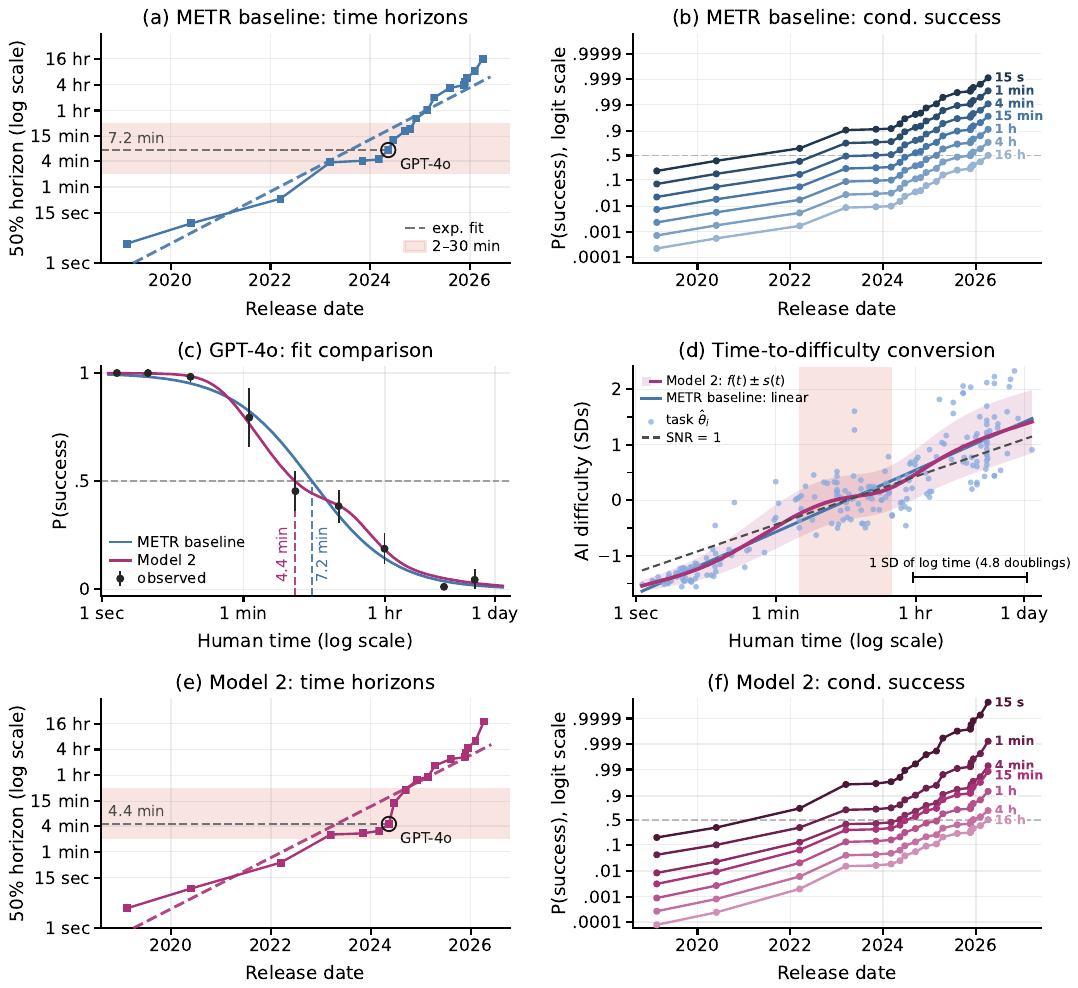
Figure 1: Summary of contributions. In this work we propose new point estimates for time horizons with an in-sample fit comparison (first column) as well as diagnostic charts for construct validity (second column). Details of how the first column was computed are described in Section 2, including a description of Model 2, and details and interpretation for the second column are in Section 3. (a) METR’s time horizon chart, computed with the baseline shared-slope logistic method. (b) A conditional success plot of based on the baseline method, which is a more complete summary of the fit than 50% time horizons. The time horizons can be read off by locating where the dotted line intersects with any plotted point, and inspecting that point’s time label. (c) An in-sample comparison of the fitted for GPT-4o. Model 2 is closer. (d) The time-to-difficulty conversion plot, using Model 2’s conversion function and fitted standard deviation . Each of the 228 points represents a task, plotted with its human time and estimated AI difficulty. The AI difficulty scale is arbitrary up to affine reparametrization, so we plot in standardized units. On these tasks log human time has a good signal to noise ratio (SNR) for AI difficulty overall, while having a notable kink from 2–30 min. The baseline assumes linearity. (e) Time horizons under Model 2. The scoring rule-based evaluations in Section 2.5 suggest that the estimates in the shaded region are particularly better; they are also the most different. (f) A conditional success plot based on Model 2. Beyond just estimating 50% time horizon, scoring rule-based evaluations also suggest that Model 2 predicts success better overall compared to the baseline, indicating that (f) may better summarize the data compared to (b).
图 1:本文贡献概览。本文提出新的时间跨度点估计,并给出样本内拟合比较(第一列),以及用于检验构念效度的诊断图(第二列)。第一列的计算细节见第 2 节,其中包括对模型 2 的说明;第二列的细节和解读见第 3 节。(a) METR 的时间跨度图,用基线的共享斜率逻辑回归方法计算。(b) 基于基线方法的条件成功率图,纵轴为 ,它比 50% 时间跨度更完整地概括了拟合结果。找到虚线与某个数据点的交点,查看该点的时间标签,就能读出时间跨度。(c) GPT-4o 拟合的 的样本内比较。模型 2 更接近。(d) 耗时—难度换算图,使用模型 2 的换算函数 和拟合的标准差 。228 个点各代表一个任务,横轴为人类耗时,纵轴为估计的 AI 难度。AI 难度的尺度只确定到仿射变换,因此我们用标准化单位作图。在这些任务上,人类耗时的对数总体上对 AI 难度有良好的信噪比(SNR),但在 2–30 分钟之间有一个明显的拐折。基线假设二者呈线性关系。(e) 模型 2 下的时间跨度。第 2.5 节基于评分规则的评估表明,阴影区域内的估计改进尤其明显,它们也是差别最大的估计。(f) 基于模型 2 的条件成功率图。除了估计 50% 时间跨度,基于评分规则的评估还表明,模型 2 对成功的整体预测优于基线,说明 (f) 可能比 (b) 更好地概括了数据。
Using METR’s public data, we reproduce[^1] METR’s time-horizon plot in Figure 1(a). Originally released in March 2025, it was updated point by point with each new AI release until ending with Claude Mythos in May 2026. The plot depicts an exponential increase in the time horizons, convincing many of AI’s overall exponential advance—the New York Times compared it to Moore’s law [Roose, 2026]—and, presumably, convincing many of AI’s future investment returns as well. Meanwhile, writing from the perspective of AI safety, Steinhardt [2026] relates it to the Keeling Curve, noting that, where the original Keeling Curve demonstrated rapidly rising atmospheric CO2 concentrations and oriented global strategy, the time-horizon plot could serve the same role for AI risk. Although the prospect of slowing down AI development became U.S. front page news in summer 2026, the time-horizon plot helped catalyze advocacy for a slowdown before then—including from figures such as Turing Award winner Yoshua Bengio and U.S. Senator Bernie Sanders.
我们用 METR 的公开数据,在图 1(a) 中复现[^1]了 METR 的时间跨度图。这张图最初发布于 2025 年 3 月,此后每有新 AI 发布就补上一个点,最后一个点是 2026 年 5 月的 Claude Mythos。图中的时间跨度呈指数增长,让许多人相信 AI 整体在指数式进步(《纽约时报》把它比作摩尔定律 [Roose, 2026]),想必也让许多人相信 AI 未来的投资回报。另一方面,Steinhardt [2026] 从 AI 安全的角度把它和基林曲线(Keeling Curve)相比:最初的基林曲线展示了大气 CO2 浓度的快速上升,并为全球战略定下了方向,时间跨度图也可能为 AI 风险起到同样的作用。放缓 AI 发展的话题在 2026 年夏天登上美国报纸头版,而在此之前,时间跨度图已经推动了放缓 AI 的倡议,倡议者包括图灵奖得主 Yoshua Bengio 和美国参议员 Bernie Sanders 等人。
[^1] Strictly speaking, we use the shared-slope logistic approach described by Barry [2026] in a METR research note.
[^1] 严格地说,我们使用的是 Barry [2026] 在一篇 METR 研究笔记中描述的共享斜率逻辑回归方法。
Unlike Moore’s law or the Keeling Curve, however, the quantity plotted on the y-axis is not a direct measurement of a physical quantity, but rather a statistical estimate which can be critiqued and improved. Indeed, the time-horizon methodology can be viewed as an application of item-response theory (IRT) techniques with human time as a covariate, allowing “software engineering capability” to be measured in the highly interpretable units of human time. This move—anchoring capability in an external scale—is the time-horizon plot’s key idea.
但与摩尔定律或基林曲线不同,这张图纵轴上的量不是对某个物理量的直接测量,而是一个统计估计,可以被批评,也可以被改进。实际上,时间跨度方法可以看作项目反应理论(IRT)技术的一种应用:以人类耗时为协变量,用人类耗时这一非常直观的单位来衡量“软件工程能力”。把能力锚定在一个外部尺度上,正是时间跨度图的核心想法。
In this work, we critique the time-horizon plot by reanalyzing METR’s data and fitting new models. Our methods and framing may be useful for any implementation of IRT methodology using an external anchoring scale. We answer two questions:
本文重新分析 METR 的数据并拟合新的模型,以此审视时间跨度图。我们的方法和框架可能适用于任何借助外部锚定尺度来实施 IRT 方法的场景。我们回答两个问题:
- What is the METR plot trying to estimate, and can a better estimate be devised? (Section 2)
- METR 图想要估计的是什么?能否设计出更好的估计?(第 2 节)
- How useful are time horizons for measuring AI capabilities? How can we diagnose this? (Section 3)
- 时间跨度在衡量 AI 能力上有多大用处?怎样诊断这一点?(第 3 节)
Though we are not the first to critique the METR plot, we are unaware of any critiques that fully claim a better estimator, or that discuss whether and under what conditions they are substantively useful.
我们不是第一个批评 METR 图的人,但据我们所知,此前还没有哪项批评完整地给出了更好的估计量,或者讨论过时间跨度是否、在什么条件下具有实质意义。
In Section 2, we improve the estimation of the time horizons on held-out data. Our main proposal is two statistical models, Model 1 and Model 2, that lead to new estimates; we quantify their improvement via scoring rule criteria. An in-sample diagnostic showing the improved fit of Model 2 relative to the baseline is presented in Figure 1(c); its time horizon estimates are in Figure 1(e).
在第 2 节中,我们改进了时间跨度在留出数据上的估计。我们的主要方案是两个统计模型,即模型 1 和模型 2,它们给出新的估计;我们用评分规则标准量化其改进。图 1(c) 给出了样本内诊断,显示模型 2 比基线拟合得更好;其时间跨度估计见图 1(e)。
Next, when and whether time horizons themselves are useful is a question of their construct validity, and it depends crucially on the relationship between a task’s human time and the latent difficulty of the task itself. Our Model 2, an item-response theory model, estimates this relationship.
其次,时间跨度本身在什么时候有用、是否有用,是它的构念效度问题,而这关键取决于任务的人类耗时与任务本身的潜在难度之间的关系。我们的模型 2 是一个项目反应理论模型,可以估计这一关系。
Therefore in Section 3, using Model 2, we propose two plots to help diagnose the construct validity of the time horizons: a “time-to-difficulty conversion” plot and a “conditional success trajectory” plot. Here “conditional” means conditional on human time.
因此,在第 3 节中,我们用模型 2 提出两种帮助诊断时间跨度构念效度的图:“耗时—难度换算”图和“条件成功率轨迹”图。这里的“条件”指以人类耗时为条件。
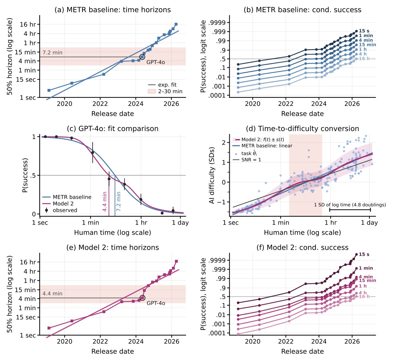
Figure 1(d) shows the time-to-difficulty conversion plot, as well as the time-to-difficulty conversion function . The plot displays estimates of each of the 228 tasks’ AI difficulty, which are non-linear in log human time. In particular, we highlight a flat region between 2–30 minutes, which also can be seen in Figure 1(c); this both raises the question of just how meaningful a time horizon jump within that region is, while also suggesting that a jump cannot have the same meaning there as it does elsewhere.
图 1(d) 展示了耗时—难度换算图,以及耗时—难度换算函数 。图中给出 228 个任务各自的 AI 难度估计,它们与人类耗时的对数呈非线性关系。我们特别指出 2–30 分钟之间有一段平坦区域,这在图 1(c) 中也能看到。这既引出一个问题:时间跨度在这一区域内的跃升究竟有多大意义;也说明这一区域内的跃升不可能与其他区域的跃升具有相同的含义。
Figures 1(b) and (f) show our conditional success trajectory plots, though we believe that Figure 1(f) is a better fit to the data than (b). This figure suggests that a time horizon jump from 4 min to 15 min may be quite small indeed.
图 1(b) 和 (f) 展示了我们的条件成功率轨迹图,我们认为图 1(f) 比 (b) 更贴合数据。这张图表明,时间跨度从 4 分钟跳到 15 分钟,实际进步可能相当小。
Finally, in Section 4 we discuss what this may mean for the time horizon methodology when potentially extended to longer tasks or applied to other domains. Overall, we view our work as providing a constructive critique for benchmarks like METR’s. We improve the time horizon estimates, while also providing a lens to assist in their interpretation.
最后,我们在第 4 节讨论,如果时间跨度方法扩展到更长的任务或应用到其他领域,这些发现可能意味着什么。总体而言,我们把本文看作对 METR 这类基准的建设性批评:既改进了时间跨度估计,也提供了一个辅助解读它的视角。
Note on terminology
术语说明
The word “model” is used in AI contexts to refer to a large language model, and in applied statistics contexts to refer to a statistical model or fit. Here, we will reserve “model” for the latter, and refer to large language models as “AIs”.
“模型”(model)一词在 AI 语境中指大语言模型,在应用统计语境中指统计模型或拟合。本文中“模型”只取后一种含义,大语言模型一律称为“AI”。
1.1 Prior work
1.1 已有工作
Abstractly, item-response theory [Baker, 2001] is the body of statistical techniques suited for jointly learning respondent ability and item difficulty from outcomes observed for an item-respondent pair. METR’s work as well as ours can be thought of as an application of this kind of theory.
抽象地说,项目反应理论 [Baker, 2001] 是一套统计技术,用于根据观测到的“题目—作答者”配对结果,同时学习作答者能力和题目难度。METR 的工作和我们的工作都可以看作这类理论的应用。
The original time-horizon measurement was introduced by Kwa et al. [2025], but the basic idea of pinning a unitless measure of ability, from IRT, to an externally interpretable quantity has previously been proposed; see, for example, the Lexile Framework for reading [Stenner, 2023].
时间跨度测量最早由 Kwa et al. [2025] 提出,但把 IRT 中无单位的能力度量锚定到一个外部可解释量上,这一基本想法以前就有人提出过,例如阅读领域的 Lexile 分级框架 [Stenner, 2023]。
Since 2025, there have been many critiques of Kwa et al. [2025] on Substack, LessWrong, and the EA Forum [shash42, 2025, Witkin, 2026, Gregory Lewis, 2026]. Statistical critiques and extensions of the time-horizon plot include Moss [2026] and METR’s own research notes [Kwa, 2026, Barry, 2026]. Substantive construct validity critiques of the time horizon concept in domains outside of software tasks include Kwa and Cheng [2025], Mertens et al. [2026].
自 2025 年以来,Substack、LessWrong 和 EA 论坛上出现了许多对 Kwa et al. [2025] 的批评 [shash42, 2025, Witkin, 2026, Gregory Lewis, 2026]。对时间跨度图的统计批评和扩展包括 Moss [2026] 以及 METR 自己的研究笔记 [Kwa, 2026, Barry, 2026]。针对软件任务之外领域中时间跨度概念的实质性构念效度批评,包括 Kwa and Cheng [2025] 和 Mertens et al. [2026]。
A major alternative measure of AI progress, similarly based on item-response theory, is the Epoch Capabilities Index [Ho et al., 2025]. Unlike the time-horizon approach, they do not pin an AI’s capability to an externally interpretable measure; this allows them to combine many benchmarks into one measure, at the cost of a less interpretable index.
另一个重要的 AI 进步度量是 Epoch 能力指数(Epoch Capabilities Index)[Ho et al., 2025],它同样基于项目反应理论。与时间跨度方法不同,它不把 AI 能力锚定到外部可解释的度量上;这样做可以把许多基准合并成一个度量,代价是指数的可解释性较差。
2 The time-horizon estimation problem
2 时间跨度的估计问题
2.1 The statistical framework
2.1 统计框架
What problem is the time-horizon plot solving? Within the framework of a statistical model, it depicts estimates of a well-specified quantity, as we shall see in Definition 2.1.
时间跨度图要解决的是什么问题?在统计模型的框架内,它描绘的是一个定义明确的量的估计,见定义 2.1。
Suppose we are able to draw tasks from some task distribution , and fix AIs . We think of the tasks as units existing in some space tasks, and AIs in AIs.
假设我们能从某个任务分布 中抽取任务 ,并固定一组 AI 。我们把任务看作空间 tasks 中的单元,把 AI 看作空间 AIs 中的单元。
Each task is associated with certain covariates, in particular associated with a human time and a task family ID. On the other hand, each AI is associated with a release date . Let be the function that associates each pair with the probability that AI solves task. Denote .
每个任务带有一些协变量,尤其是人类耗时 和任务族 ID。另一方面,每个 AI 带有一个发布日期 。设 是把每个 配对映射到该 AI 完成该任务的概率的函数,记 。
Given and , assume we have access to a mechanism to draw iid samples , such that , which models multiple trials of re-running the AI on the same prompt. Here represents the runs where attempts , and is the success or failure of the th run.
给定 和 ,假设我们有一种机制可以抽取独立同分布样本 ,满足 ,用来刻画在同一提示上多次重跑 AI 的试验。这里 表示 尝试 的 次运行, 是第 次运行的成功或失败。
(Despite this iid assumption, approximation errors in the functional form of any practical model specification will induce correlation among trials in the runset even for the same AI-task pair when conditioning on latent features. We return to this point when introducing our Model 2.)
(尽管有这一独立同分布假设,任何实际模型设定在函数形式上的近似误差,都会使运行集 中的各次试验在以潜在特征为条件时仍然相关,即使是同一个 AI—任务配对也不例外。介绍模型 2 时我们会回到这一点。)
Define the success curve . We make the structural assumption that, for our chosen AIs and task distribution , this function is strictly monotone decreasing in , so that its inverse is always defined.
定义成功曲线 。我们作一个结构性假设:对选定的 AI 和任务分布 ,这个函数关于 严格单调递减,因此其反函数总是有定义的。
Now, we can define the oracle quantity we would like to estimate, from the data and .
现在可以定义我们想从数据 和 中估计的理想量。
Definition 2.1.
定义 2.1.
For , the -time horizon of is
对 , 的 -时间跨度为
This is the human time of tasks from that can solve with probability . To learn this quantity for each AI it suffices, therefore, to learn the regression function , for each . The time-horizon plots of Figures 1(a) and (e) are then a scatter of points .
这是 能以概率 完成的、来自 的任务的人类耗时。因此,要得到每个 AI 的这个量,只需对每个 学习回归函数 。图 1(a) 和 (e) 的时间跨度图就是点 的散点图。
Importantly for the interpretation of the METR plot, the release dates are used nowhere in the model; the observed exponential growth is entirely empirical and we do not challenge it here.
对解读 METR 图来说很重要的一点是:模型中完全没有用到发布日期 ;观察到的指数增长完全是经验结果,本文不对它提出质疑。
2.2 Implementing the framework
2.2 框架的实施
In order to implement this framework in the real world, we require the following ingredients: tasks , thought to be sampled from some relevant task distribution ; a setup for humans and AIs to attempt the tasks, and hence measure each task’s human time, , as well as the task-AI success indicators for each task-AI pair ; a technique for estimating the marginal success probability for the th AI, with confidence intervals; and finally, a method for evaluating whether our estimate had good performance.
要在现实中实施这一框架,需要以下几样东西:任务 ,可以认为它们是从某个相关任务分布 中抽样得到的;一套让人类和 AI 尝试这些任务的设置,从而测出每个任务的人类耗时 ,以及每个任务—AI 配对 的成功指示 ;一种估计第 个 AI 边际成功概率 并给出置信区间的技术;最后,一种评估估计表现好坏的方法。
In this section, we summarize strategies for each of these implementation components. In particular, we summarize METR’s approach for the first two components; see Kwa et al. [2025] for a fuller description. For the last two components (estimation and evaluation), we summarize general principles here and defer fuller exposition to Sections 2.3 and 2.4.
本节概述实施上述各部分的策略。前两部分我们概述 METR 的做法,更完整的描述见 Kwa et al. [2025]。后两部分(估计与评估)我们在这里概述一般原则,详细说明放在第 2.3 和 2.4 节。
Designing the tasks.
设计任务。
METR designed 228 tasks in their Time Horizon 1.1 framework, which were broadly software engineering relevant tasks such as “implement this function” or “train this classifier” written as a set of instructions, together with an automated function that scores the result. Each task was a member of one of three “task suites” with a unifying theme; each task was further classified into a task_family, of which there were 79.
METR 在其 Time Horizon 1.1 框架中设计了 228 个任务,大体上都是与软件工程相关的任务,例如“实现这个函数”或“训练这个分类器”,以一组指令的形式写成,并配有一个自动给结果打分的函数。每个任务属于三个有统一主题的“任务套件”之一;每个任务还被进一步归入一个任务族(task_family),共有 79 个任务族。
Attempting the tasks.
尝试任务。
For each task, a shared setup was used for both humans and AIs to attempt the task. This was concretely three things per task: a set of task instructions, a field to input the task solution, and a scorer function to judge success or failure.
每个任务都有一套人类和 AI 共用的尝试设置,具体包括三样东西:一组任务指令、一个填写任务答案的输入框,以及一个判断成功或失败的评分函数。
On the human side, multiple software engineers were recruited to attempt each task while being timed (typically attempts per task); on attempts where the scorer judged a success, their time measurements were combined using the geometric mean. This value is called the human time of the task (METR’s “task length”), which we denote for . However, these measurements were unobtainable or deemed invalid (e.g. too few successes) for 29% of the tasks, and in those cases, an expert’s value is used instead to set as .
在人类一侧,每个任务招募多名软件工程师计时完成(通常每个任务约 次尝试);对评分函数判为成功的尝试,用几何平均合并其用时。这个值称为任务的人类耗时(METR 所说的“任务长度”),对 记为 。不过,有 29% 的任务无法得到这样的测量值,或测量值被判为无效(例如成功次数太少),这些情况下改用专家给出的估值作为 。
On the AI side, the th AI was provided the instructions for as a prompt and run autonomously times, and the scorer’s output recorded as for each run. Note that we ignore the time AIs take to complete tasks.
在 AI 一侧,把 的指令作为提示交给第 个 AI,让它自主运行 次,并把每次运行的评分输出记为 。注意,我们不考虑 AI 完成任务所用的时间。
Fitting models and estimating time horizons.
拟合模型并估计时间跨度。
Here we summarize general principles for fitting models; concrete approaches are detailed in Section 2.3. The framework of Section 2.1 allows us to precisely define the statistical problem at hand: we want good estimates for , especially and , for each . METR’s original approach, as well as ours, will be to first obtain estimates for and then invert the function according to Definition 2.1. These per-AI success curves , also called “characteristic curves” in item-response theory, can be estimated in any way in principle, as long as they are ultimately evaluated with held-out data.
这里概述拟合模型的一般原则,具体做法详见第 2.3 节。第 2.1 节的框架让我们可以精确定义眼前的统计问题:我们希望对每个 得到 的良好估计,尤其是 和 。METR 最初的做法和我们的做法一样,都是先估计 ,再按定义 2.1 求反函数。这些逐 AI 的成功曲线 在项目反应理论中也称为“特征曲线”,原则上可以用任何方式估计,只要最终用留出数据来评估。
These approaches are all based on the same tabular dataset, where a row consists of the AI’s ID , the task’s index , the run index , the success indicator for the AI’s attempt on that task, and finally the task’s human time —we do not use the AI’s release date for fitting, but only for plotting.
这些做法都基于同一个表格数据集,每一行包括 AI 的 ID 、任务索引 、运行索引 、该 AI 在该任务上这次尝试的成功指示 ,以及任务的人类耗时 。我们不用 AI 的发布日期 做拟合,只用它作图。
Evaluating models.
评估模型。
Finally, we summarize general principles for evaluating models; our evaluation metrics are defined in Section 2.4, with results in Section 2.5. Essentially, given estimates for the success curves , we compute these metrics to adjudicate between the different estimates and select the best. Our metrics consist of proper scoring rules and Murphy diagrams [Dimitriadis et al., 2023], which we computed with 5-fold cross validation; this can be thought of as an extension of the evaluations in Barry [2026]. We also plot in-sample visual diagnostics for our estimates against empirical frequencies to assess the functional form, as done by Kwa et al. [2026] in their Figure 4.
最后,我们概述评估模型的一般原则;评估指标在第 2.4 节定义,结果见第 2.5 节。简单地说,给定成功曲线的估计 ,我们计算这些指标,在不同估计之间做出裁决并选出最好的。我们的指标由适当评分规则和墨菲图(Murphy diagram)[Dimitriadis et al., 2023] 组成,用 5 折交叉验证计算;这可以看作对 Barry [2026] 中评估的扩展。我们还像 Kwa et al. [2026] 的图 4 那样,画出 估计与经验频率对比的样本内可视化诊断,以评估函数形式。
2.3 Model specifications
2.3 模型设定
In this section, we list the four main model specifications we ran. By model specification, we mean a model family and fitting procedure for the success curves . The first two were proposed by METR, and the last two are our contribution.
本节列出我们运行的四种主要模型设定。所谓模型设定,是指成功曲线 的模型族加上拟合过程。前两种由 METR 提出,后两种是我们的贡献。
Logistic regression.
逻辑回归。
This is the original headline model specification used by METR. For each , we assume for the log-linear model
这是 METR 最初用于主要结果的模型设定。对每个 ,我们假设 服从对数线性模型
with . We estimate the parameters , for each with logistic regression, i.e. minimizing binary cross entropy, using as covariates. When the cross-entropy is unweighted, this is formally equivalent to maximum likelihood with the generative model independently for all .
其中 。我们以 为协变量,用逻辑回归(即最小化二元交叉熵)估计每个 的参数 、。交叉熵不加权时,这在形式上等价于在生成模型“对所有 独立地有 ”下做最大似然估计。
Such an independence assumption is certainly wrong, but this does not necessarily mean that the success curves are wrong. Also, tasks in a shared task family have correlated behavior, so following Kwa et al. [2025], the effect of large families was downweighted in training by using the sqrt-family weighting described in Section 2.4.1 on the cross-entropy loss.
这样的独立性假设肯定是错的,但这并不一定意味着成功曲线是错的。另外,同一任务族内的任务表现相关,因此我们沿用 Kwa et al. [2025] 的做法,在交叉熵损失上使用第 2.4.1 节描述的平方根任务族加权(sqrt-family weighting),降低大任务族在训练中的影响。
Logistic regression with shared slope (our baseline).
共享斜率的逻辑回归(我们的基线)。
This specification was tried by Barry [2026] in work for METR. It is the same as the previous, except we assume for that
Barry [2026] 在为 METR 做的工作中尝试过这一设定。它与前一个设定相同,只是假设 满足
for a fixed common to each AI. Again, an unweighted fit is equivalent to maximum likelihood on a model where all the are independent conditionally on the human times .
其中 是所有 AI 共用的固定值。同样,不加权的拟合等价于在“以人类耗时 为条件、所有 相互独立”的模型上做最大似然估计。
Barry [2026] observes it has better performance in cross-validation on both Brier score and marginal log score, with sqrt-family weighting; we replicate this finding, and in fact it beats METR’s model spec on all but one of the 12 metrics in our proper scoring suite (Section 2.5). We hence use this spec as our performance baseline, rather than the logistic regression spec. The time horizons from this fit were displayed in Figure 1(a).
Barry [2026] 观察到,在平方根任务族加权下,它在交叉验证的 Brier 分数和边际对数分数上都表现更好;我们复现了这一结果,而且在我们的适当评分规则套件的 12 项指标中,它有 11 项胜过 METR 的模型设定(第 2.5 节)。因此我们用这一设定而不是逻辑回归设定作为性能基线。图 1(a) 展示的就是这一拟合得到的时间跨度。
Model 1: Shared monotone spline, with shared slope.
模型 1:共享单调样条,共享斜率。
This specification just replaces the linear dependence on with a monotone function. We assume for that
这一设定只是把对 的线性依赖换成一个单调函数。我们假设 满足
We take to be a monotone natural cubic spline; specifically, a monotone natural cubic I-spline with nonnegative coefficients with 4 interior knots. Additionally, because of non-uniqueness with respect to affine transformations of where , we make the identifiability assumption and . Then we fit with binary cross entropy, with sqrt-family weighting; again, an unweighted fit is equivalent to maximum likelihood on a model where all the are independent conditionally on the human times .
我们取 为单调自然三次样条,具体来说是系数非负、有 4 个内部节点的单调自然三次 I 样条。此外,由于 在仿射变换 ()下不唯一,我们作可识别性假设 和 。然后用平方根任务族加权的二元交叉熵拟合;同样,不加权的拟合等价于在“以人类耗时 为条件、所有 相互独立”的模型上做最大似然估计。
A monotone spline-based approach was previously considered by METR in Kwa [2026], and attempted in Barry [2026], but did not beat the baseline; this was likely because they were separate splines, rather than shared.
METR 此前在 Kwa [2026] 中考虑过基于单调样条的方法,Barry [2026] 也尝试过,但都没有胜过基线;这很可能是因为他们用的是各自独立的样条,而不是共享样条。
The single shared shape gives this specification its interpretation. It is an estimate of how AI difficulty varies with human time, common to all the AIs. Using item-response theory in Model 2, we can extend this interpretation further.
单一的共享形状 赋予了这个设定可解释性:它估计的是 AI 难度如何随人类耗时变化,并且对所有 AI 通用。借助模型 2 中的项目反应理论,我们可以把这种解释进一步扩展。
Model 2: Explanatory IRT with family effects and overdispersion.
模型 2:带任务族效应和过度离散的解释性 IRT。
This specification is a fully generative model for all the ’s. We fit it with maximum likelihood, and subsequently derive the success curves. This model involves task families; let index the families, and let be the task family of . Let be the geometric mean of human times in .
这一设定是所有 的完整生成模型 。我们用最大似然拟合它,再从中推导成功曲线。这个模型涉及任务族:令 索引任务族, 为 所属的任务族, 为 中人类耗时的几何平均。
In this model, each carries a latent difficulty . Define
在这个模型中,每个 带有一个潜在难度 。定义
for the success probability of a single run conditional on the difficulties. We model this as
为以难度为条件时单次运行的成功概率。我们把它建模为
where the is shared among all AIs . The latent difficulty is modeled as
其中 由所有 AI 共享。潜在难度建模为
for some mean function , family variance , and idiosyncratic variance .
其中 是均值函数, 是任务族方差, 是任务自身的方差。
Even though we assume are iid, we do not model them as independent conditional on , since the pair is not a complete summary of the AI-task interaction, and conditioning on these induces correlation between trials for each AI-task pair. Hence we introduce a correlation parameter shared by all AIs, put , and model the final probability as drawn from
尽管我们假设 独立同分布,但我们并不把它们建模为以 为条件相互独立,因为 这一对数并不能完整概括 AI 与任务之间的交互,以它们为条件会在每个 AI—任务配对的各次试验之间引入相关性。因此,我们引入一个所有 AI 共享的相关参数 ,令 ,并把最终概率 建模为从下式中抽取:
so that is beta-binomial, allowing us to model it with higher variance than if it were only binomial (hence the name “overdispersion”). The source of this higher variance is the correlation for .
这样 服从贝塔二项分布,使我们能用比单纯二项分布更大的方差来建模(“过度离散”一名即由此而来)。方差增大的来源是相关性 ()。
Fitting maximum likelihood under this model is not trivial. We implemented an EM algorithm and approximated the integrals with Gauss-Hermite quadrature. Note that, similar to Model 1, the likelihood is invariant to affine transformations of , so we fix the scale with identifiability assumptions on .
在这个模型下做最大似然拟合并不简单。我们实现了 EM 算法,并用高斯—埃尔米特求积近似积分。注意,与模型 1 类似,似然对 的仿射变换不变,因此我们通过对 的可识别性假设来固定尺度。
To compute under this model, we must marginalize over the random effects:
要在这个模型下计算 ,必须对随机效应求边际:
where evaluating at is the convention for a fresh task from a fresh family whose mean human time is . We evaluate this by quadrature and invert numerically for .
其中在 处取 的值,对应的约定是:一个来自新任务族的新任务,该任务族的平均人类耗时为 。我们用数值求积计算它,再数值求逆得到 。
Remarks on Model 2.
关于模型 2 的说明。
This is an item-response theory model. Specifically, it is a kind of 1PL Rasch model due to the shared . In general, item-response theory uses latent variables to model the success probability of a respondent on a test item. It captures correlations between responses that share a respondent or an item by modeling a shared latent trait that connects them—a student’s ability in a standardized testing setting, or, in our case, the task difficulty , which connects and for .
这是一个项目反应理论模型。具体来说,由于 共享,它属于单参数(1PL)Rasch 模型。一般而言,项目反应理论用潜变量来建模作答者在某道测试题上的成功概率。对于共享同一作答者或同一题目的作答结果,它通过建模一个把它们联系起来的共享潜在特质来刻画其相关性:在标准化考试中,这个特质是学生的能力;在我们这里,则是任务难度 ,它把 时的 和 联系起来。
It is an explanatory IRT here because is regressed on the task’s observed covariates: human time and task family, which “explain” the values of . We use the same family of monotone spline as in Model 1, with the same identifiability assumption, and take and to each be the exponential of a natural cubic spline with 2 interior knots.
这里之所以是解释性 IRT,是因为 对任务的观测协变量(人类耗时和任务族)做了回归,由这些协变量“解释” 的取值。我们使用与模型 1 相同的单调样条族 和相同的可识别性假设,并把 和 各取为一个有 2 个内部节点的自然三次样条的指数。
Like in Model 1, the mean function accounts for non-linearities between difficulty and log human time, while the individual and family effects account for possible spread in task difficulties from their mean. In particular, the family effect accounts for correlations among tasks within a family, without the heuristic sqrt-family reweighting.
与模型 1 一样,均值函数 刻画难度与人类耗时对数之间的非线性,而任务个体效应和任务族效应刻画任务难度围绕均值可能的分散。尤其是,任务族效应 刻画了同一任务族内任务之间的相关性,不再需要启发式的平方根任务族重加权。
We account for dependence within the runset via the correlation parameter . In the data, this dependence is actually substantial: assuming the generative model implied by the baseline spec, where all are independent, then assuming the fitted were correct, we would predict that of vectors were unanimous. However, it is actually 83% of them. The correlation parameter affects the final fit by downweighting AI-task pairs with many runs, as they carry redundant information.
我们通过相关参数 处理运行集 内部的依赖。在数据中,这种依赖实际上相当大:假设基线设定所隐含的生成模型成立,即所有 相互独立,再假设拟合出的 是正确的,那么我们会预测约 的向量 各次结果一致。但实际上有 83% 一致。相关参数会降低运行次数多的 AI—任务配对的权重,因为这些配对携带的信息是冗余的,从而影响最终拟合。
2.4 Evaluation with proper scoring rules
2.4 用适当评分规则评估
In this section, let index modeling approaches, each of which supplies a success curve for every , which we assume to be monotone decreasing in , so that the time horizons are well defined. Let
本节中,令 索引各种建模方法,每种方法为每个 提供一条成功曲线 ,我们假设它关于 单调递减,从而时间跨度 有良好定义。令
collect, respectively, every run outcome in the table and every human time, so that the dataset is the pair .
分别汇集表中所有运行结果和所有人类耗时,于是数据集就是 这一对。
A scoring rule is then a function of the data and the approach. We use the four scores below. The first three (marginal log score, Brier score, and elementary score) are oriented so that smaller is better, and we report each divided by its total weight .
评分规则是数据和方法的函数 。我们使用下面四种分数。前三种(边际对数分数、Brier 分数和基本分数)都是越小越好,我们报告时把每种分数除以其总权重 。
Marginal log score.
边际对数分数。
Also known as binary cross entropy. Writing for the predicted success probability, let
也就是二元交叉熵。把预测成功概率记为 ,令
for some weights . This score only depends on through the functions .
其中 为权重。这个分数只通过函数 依赖于 。
With all the weights equal to 1, minimizing this score in training is identical to maximizing log-likelihood when every is assumed drawn independently. Even though such a model is certainly not a good fit in our application, that does not necessarily imply that the resulting success-curve functions are not a good fit.
当所有权重都为 1 时,在训练中最小化这个分数,等同于在假设每个 独立抽取时最大化对数似然。尽管这样的模型在我们的应用中肯定拟合得不好,但这并不一定意味着由此得到的成功曲线函数 拟合得不好。
Brier score.
Brier 分数。
With the same definitions as in marginal log score, let
沿用边际对数分数中的定义,令
Like the marginal log score, this only depends on through the functions .
与边际对数分数一样,它只通过函数 依赖于 。
Elementary binary score at level .
水平 下的基本二元分数。
For , define
对 ,定义
assuming no ties between and . This score only depends on through the time horizons . In other words, this score directly measures the quality of the time horizon estimates.
这里假设 与 之间没有相等的情况。这个分数只通过时间跨度 依赖于 。换句话说,它直接衡量时间跨度估计的质量。
These scores are elementary in the sense that every proper scoring rule for a binary outcome is a nonnegative mixture of them [Schervish, 1989]; in particular, the Brier score satisfies . The curve is the Murphy diagram of [Ehm et al., 2016], which we also plot; one specification dominating another at every on the plot implies dominance under every proper score.
这些分数之所以称为“基本”分数,是因为二元结果的任何适当评分规则都是它们的非负混合 [Schervish, 1989];特别地,Brier 分数满足 。曲线 就是 的墨菲图 [Ehm et al., 2016],我们也把它画了出来;如果在图上的每个 处,一个设定都优于另一个,那么它在每种适当评分规则下都占优。
At a single , these scores are noisy, so for our evaluations we report the smoothed score . This can be thought of then as measuring an average of the quality of the time horizons within that window.
在单个 处,这些分数噪声很大,因此评估时我们报告平滑后的分数 。可以认为它衡量的是该窗口内时间跨度 的平均质量。
Full log-likelihood.
完整对数似然。
When a generative model is available, we can use this score. The (full) log-likelihood has the typical definition of
有生成模型时,可以使用这个分数。(完整)对数似然按通常方式定义为
This scores the entire model , including correlations between the . In particular, it is possible to do poorly in estimating the but still do well on the full log-likelihood.
它给整个模型 打分,包括各个 之间的相关性。特别地,一个模型可能对 估计得很差,却在完整对数似然上得分很好。
2.4.1 Evaluation weights
2.4.1 评估权重
The choice of weights essentially is a choice of what distribution of prediction problems we would like to average over; it does not depend on the run index .
选择权重 ,本质上是选择我们想在什么样的预测问题分布上取平均;权重与运行索引 无关。
Writing for the task_family of and for the number of scored tasks belonging to family , we use the following three weightings:
把 所属的任务族记为 ,把属于任务族 的已评分任务数记为 ,我们使用以下三种加权:
All of these schemes weight the AIs uniformly, but not the tasks. The equal task weighting targets a uniformly drawn task, adjusting for unequal numbers of runs. The equal family weighting instead targets a uniformly drawn task family, adjusting for unequal numbers of tasks in the family. Finally, the sqrt-family weighting is an intermediate used by METR for both fitting and evaluating their models.
这些方案对各 AI 的权重都是均匀的,对任务则不是。等任务加权(equal-task)以均匀抽取的任务为目标,校正运行次数不等的问题。等任务族加权(equal-family)则以均匀抽取的任务族为目标,校正各任务族任务数不等的问题。平方根任务族加权(sqrt-family)介于两者之间,METR 在拟合和评估模型时都使用它。
It is also possible to define versions of the scoring rules specific to each , by restricting the sum over to that single AI.
也可以为每个 单独定义评分规则,只需把对 的求和限制在这一个 AI 上。
2.4.2 A suite of proper scoring rule metrics
2.4.2 一套适当评分规则指标
Our main numerical measure of model quality is based on crossing the above scoring rules with the weighting schemes, under 5-fold cross validation on task families. That is, we split the 79 task families into 5 approximately equally sized folds, and then evaluate marginal log score, Brier score, and the smoothed elementary binary score at and on each fold using a model trained from data out-of-fold. Crossing these four scores with the three weighting schemes gives 12 proper scoring rule metrics.
我们衡量模型质量的主要数值指标,是把上述评分规则与各种加权方案交叉组合,并在任务族上做 5 折交叉验证。也就是说,我们把 79 个任务族分成大小大致相等的 5 折,在每一折上用折外数据训练的模型,计算边际对数分数、Brier 分数,以及 和 处的平滑基本二元分数。四种分数与三种加权方案交叉,得到 12 项适当评分规则指标。
2.5 Fit results and diagnostics
2.5 拟合结果与诊断
The results of the scoring rule metrics are displayed in Figure 2, showing that the point estimates for our methods dominate the baseline on all metrics. Our chosen baseline itself dominates the original logistic regression specification on all metrics except one, namely equal-task , so we do not report its results.
评分规则指标的结果见图 2:我们方法的点估计在所有指标上都优于基线。我们选用的基线本身,在除等任务加权 之外的所有指标上都优于最初的逻辑回归设定,因此我们不再报告后者的结果。
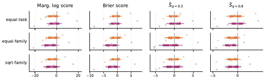
Figure 2: Models 1 and 2 against the baseline across the scoring-rule suite. Each panel shows the paired difference in weighted per-run score between our model and the baseline. (Left is better for our models.) The confidence intervals use family as the unit , at two nested levels: 80% thick, 95% thin. Point estimates for both of our models dominate the baseline at every displayed metric and weighting.
图 2:在评分规则套件上比较模型 1、模型 2 与基线。每个子图显示我们的模型与基线在加权单次运行分数上的配对差值(越靠左,我们的模型越好)。置信区间以任务族为单位(),分两个嵌套水平:粗线为 80%,细线为 95%。在图中所示的每项指标和每种加权下,我们两个模型的点估计都优于基线。
We also plot the Murphy diagrams in Figure 3. For , the baseline seems to be nearly dominated, partly explaining why we get favorable performance on Brier score and marginal log score, as they are just weighted mixtures of points on the Murphy diagram.
我们还在图 3 中画出了墨菲图。当 时,基线几乎全面落后,这部分解释了为什么我们在 Brier 分数和边际对数分数上表现更好,因为这两种分数正是墨菲图上各点的加权混合。
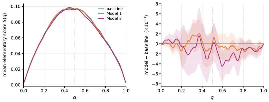
Figure 3: Murphy diagrams of Models 1 and 2 against the baseline, with equal-family weighting. Left: Murphy diagrams of the baseline, Model 1, and Model 2. Right: Each model’s paired difference from the baseline (), with its 95% band based on family units. For display, these curves are smoothed by a centered rolling mean over the -grid ( wide in ).
图 3:等任务族加权下模型 1、模型 2 与基线的墨菲图。左:基线、模型 1 和模型 2 的墨菲图。右:各模型与基线的配对差值(),以及基于 个任务族单位的 95% 置信带。为便于展示,这些曲线在 网格上做了居中滚动平均平滑(窗口宽约 )。
Additionally, we plot in-sample diagnostics in Figure 4 for six AIs with time horizons of 2–15 min. The shape of Models 1 and 2 bends to follow a flat region through roughly 2–30 minutes whose tasks Figure 1(d) shows have roughly equal difficulty, while the log-linear baseline is forced to cut straight through. Our fits substantially change the 50% time horizon estimates for these AIs, some of which go outside the original METR plot’s 95% confidence intervals.
此外,我们在图 4 中给出了六个时间跨度为 2–15 分钟的 AI 的样本内诊断。模型 1 和模型 2 的形状弯折过来,贴合大约 2–30 分钟的一段平坦区域(图 1(d) 显示这段区域内的任务难度大致相同),而对数线性的基线只能直线穿过。我们的拟合大幅改变了这些 AI 的 50% 时间跨度估计,其中一些甚至落到了原始 METR 图的 95% 置信区间之外。
A version separated by AIs is shown in the Appendix as Figure 9, showing that a large amount of the gain in the metrics was due to improvement in estimates for AIs with time horizons of 2–15 min, such as these six, which were most affected by the flat region of tasks with human time 2–30 min, as shown in Figure 1(d).
附录图 9 给出了按 AI 拆分的版本,显示指标上的提升很大一部分来自时间跨度为 2–15 分钟的 AI(例如这六个)的估计改进;如图 1(d) 所示,受人类耗时 2–30 分钟这段平坦区域影响最大的正是这些 AI。
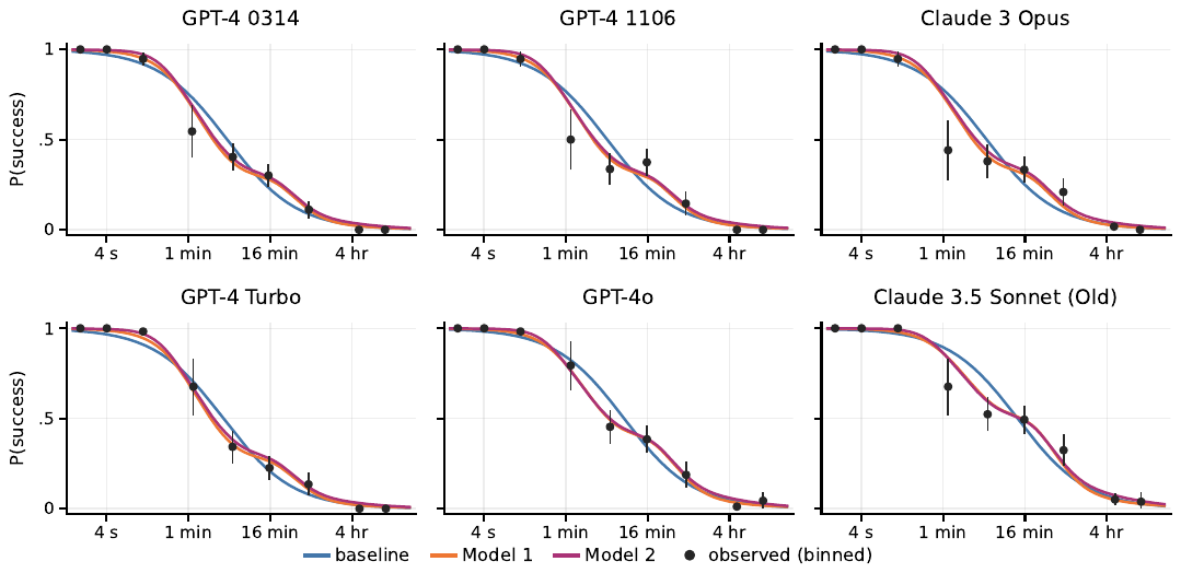
Figure 4: In-sample fitted against binned observed frequencies, for six AIs with time horizons of 2–15 min. Black points pool each AI’s runs within factor-4 human-time bins—width two in minutes, with bin centers at 1 min, 4 min, 16 min, etc—plotted at the run-weighted mean human time within the bin. (The points are therefore unevenly spaced). Vertical bars are 95% Wald intervals over the bin’s runs.
图 4:六个时间跨度为 2–15 分钟的 AI 的样本内拟合 与分箱观测频率的对比。黑点把每个 AI 的运行按人类耗时以 4 倍为间隔分箱(在以分钟为单位的 尺度上宽度为 2,箱中心为 1 分钟、4 分钟、16 分钟等),画在箱内按运行次数加权的平均人类耗时处(因此各点间距不均)。竖线是基于箱内 次运行的 95% Wald 区间 。
3 Diagnostics for construct validity
3 构念效度诊断
3.1 Construct validity for capability anchoring
3.1 能力锚定的构念效度
We loosely define construct validity to be a property of a statistical estimand—whether, at the population level, it measures the construct that we wish it to measure. For example, when reading the METR plot one might assume, implicitly, that the construct of “AI software development capabilities” is well captured by the estimand of “50% time horizons on METR’s task suite”. But whether this is actually the case depends on how the human time of the suite’s tasks relates to their difficulty for an AI—the relationship between human time and AI difficulty.
我们粗略地把构念效度定义为统计估计目标(estimand)的一种性质:在总体层面上,它是否衡量了我们希望它衡量的构念。例如,读 METR 图时,人们可能默认“AI 软件开发能力”这一构念被“METR 任务套件上的 50% 时间跨度”这一估计目标很好地刻画了。但实际是否如此,取决于套件中任务的人类耗时与它们对 AI 的难度之间是什么关系,即人类耗时与 AI 难度的关系。
This consideration applies to using any interpretable, external feature besides human time. Let us refer to this key idea of time horizons as “capability anchoring”. Capability anchoring is in principle applicable to any benchmark dataset where AIs are set up to attempt tasks, or perhaps only a subset of them, and where the tasks have external annotations . The general approach is then roughly abstractable to the following steps:
除了人类耗时,使用任何可解释的外部特征都要考虑这一点。我们把时间跨度的这一核心想法称为“能力锚定”(capability anchoring)。原则上,能力锚定适用于任何这样的基准数据集: 个 AI 尝试 个任务(也可能只尝试其中一部分),并且这 个任务带有外部标注 。一般做法大致可以抽象为以下几步:
- Learn task difficulties and AI capabilities jointly with some method (say, IRT), and hence learn a function as our best predictor of the chance that AI will succeed at task .
- Regress the learned task difficulties on the external annotations to learn a mapping from annotation to difficulty.
- Define AI ’s “anchored capability” as a 50% horizon, via , where solves . (This is the annotation value whose predicted difficulty gives AI an even chance of success.) Use the “anchored capability” as an interpretable scale for the AI’s capability.
- 用某种方法(比如 IRT)同时学习任务难度 和 AI 能力 ,从而学到一个函数 ,作为 AI 完成任务 的概率的最佳预测。
- 把学到的任务难度 对外部标注 做回归,学到一个从标注到难度的映射 。
- 把 AI 的“锚定能力”定义为 50% 跨度,即 ,其中 满足 。(这是这样一个标注值:按它预测出的难度,AI 成功与失败的机会各半。)用“锚定能力”作为 AI 能力的可解释尺度。
In our setting, it is possible actually to follow these steps by using a Rasch model to perform Step 1 and a monotone spline to fit in Step 2. The function then essentially follows the specification of Model 1 but with a different way of learning the parameters; we found the result to be nearly competitive with both Model 1 and 2. However, we prefer to use these steps as a conceptual way to understand methods for capability anchoring: Model 1 and the baseline implicitly perform Steps 1 and 2 jointly, though the baseline assumes that the mapping is linear in log human time. Model 2’s EM algorithm alternates between Step 1 and Step 2 in the course of fitting, using the fitted to improve the estimates of difficulties and capabilities and then using those estimates to re-fit .
在我们的设定中,确实可以按这些步骤来做:第 1 步用 Rasch 模型,第 2 步用单调样条拟合 。这样得到的函数 基本上就是模型 1 的设定,只是参数的学习方式不同;我们发现其结果与模型 1 和模型 2 都相差无几。不过,我们更愿意把这些步骤当作理解能力锚定方法的概念框架:模型 1 和基线隐含地把第 1 步和第 2 步合在一起做,只是基线假设映射 关于人类耗时的对数是线性的。模型 2 的 EM 算法在拟合过程中交替执行第 1 步和第 2 步,用拟合出的 改进难度和能力的估计,再用这些估计重新拟合 。
Given this abstraction for capability anchoring, we posit that the construct validity of time horizons and capability anchoring in general comes from affirmative answers to the following “checklist” questions:
有了能力锚定的这一抽象,我们认为,时间跨度乃至一般能力锚定的构念效度,来自对以下“清单”问题的肯定回答:
- Are the tasks representative of real tasks—does solving them mean the AI is “capable” in the sense that we wish?
- Do two numbers and the function model the difficulty-capability interaction well, or do more numbers/different specifications fit significantly better?
- Does the annotation have an objective meaning? Is it the same objective meaning across different tasks? Does this objective meaning capture a desired construct? Relative to this objective meaning, is the annotation measured well, and if not, can we account for it?
- (Predictiveness) Are the task annotations predictive of the difficulties, and hence AI success of the tasks?
- (Comparability) Is the relationship between the annotation and the difficulties different depending on the annotation? For anchored capabilities, can we interpret equal differences among AIs equally? If not, can we account for it?
- 这些任务是否代表真实任务?完成它们是否意味着 AI 具备我们所说的那种“能力”?
- 两个数 加上函数 ,能否很好地刻画难度与能力之间的交互?还是用更多的数或不同的设定会拟合得明显更好?
- 标注是否有客观含义?不同任务上的客观含义是否相同?这种客观含义是否刻画了想要的构念?相对于这种客观含义,标注是否测得准确?如果不准确,能否加以校正?
- (预测性)任务标注能否预测任务难度,从而预测 AI 在任务上的成功?
- (可比性)标注与难度之间的关系是否随标注取值而变化?对于锚定能力,AI 之间相等的差距能否作同等解读?如果不能,能否加以校正?
Many critiques of the construct validity of time horizons address the first three questions. In this work, we simply assume that answers to the first three questions are affirmative. Our diagnostic plots are then comparatively narrow—only addressing the last two questions of predictiveness and comparability.
许多对时间跨度构念效度的批评针对的是前三个问题。本文直接假定前三个问题的答案都是肯定的。因此我们的诊断图范围相对较窄,只处理后两个问题,即预测性和可比性。
The issue raised by predictiveness is this. In the setting of Section 2.1, suppose AIs A and B have 50% time horizons and , with , representing a large jump in the time horizon. Interpreting this as a large increase in capabilities seems misleading if both and are small, i.e. if human time is not predictive of AI success in . This would be reflected by and being flat in that region.
预测性引出的问题是这样的。在第 2.1 节的设定下,假设 AI A 和 B 的 50% 时间跨度分别为 和 ,且 ,即时间跨度有一次大的跃升。如果 和 都很小,也就是说在 区间内人类耗时不能预测 AI 的成功,那么把这次跃升解读为能力的大幅提高就是误导性的。这种情况会表现为 和 在该区间内都是平的。
For comparability, suppose AIs C and D have 50% time horizons and , with while . This represents the same multiplier of time horizon, and hence the same jump on the time-horizon plot, but it may not mean the same thing if the relationship between human time and AI difficulty changes significantly.
至于可比性,假设 AI C 和 D 的 50% 时间跨度分别为 和 ,,同时 。这代表时间跨度的倍数相同,因而在时间跨度图上跃升幅度相同;但如果人类耗时与 AI 难度之间的关系发生了明显变化,两者的含义可能并不相同。
Predictiveness has previously been recognized as an issue in general. When METR attempted to replicate its analysis on new task suites, they found low correlation between human time and AI success in the case of video understanding tasks [Kwa and Cheng, 2025], and diagnosed a lack of “soundness of the time horizon metric” in that setting. Later, Mertens et al. [2026] found low predictiveness between human time and AI success on a broad range of economically relevant tasks. However, just because predictiveness is low does not mean 1-dimensional difficulties are not useful, and comparability does not seem to previously have been discussed.
预测性问题此前已被普遍认识到。METR 尝试在新的任务套件上复现其分析时发现,在视频理解任务上,人类耗时与 AI 成功之间相关性很低 [Kwa and Cheng, 2025],并判断“时间跨度指标的可靠性”在该场景下不足。后来,Mertens et al. [2026] 在大量具有经济意义的任务上发现,人类耗时对 AI 成功的预测性很低。不过,预测性低并不意味着一维难度没有用处;而可比性问题此前似乎还没有人讨论过。
On METR’s software tasks suite, predictiveness is strong. Using diagnostic plots, in this work we have found that it is locally weak in the 2–30 min region, raising a comparability issue with other regions. Below we illustrate the use of our two diagnostic plots, the time-to-difficulty conversion and the conditional success plots, to assess both predictiveness and comparability, and hence calibrate our interpretations of the time horizons.
在 METR 的软件任务套件上,预测性很强。借助诊断图,本文发现预测性在 2–30 分钟区域局部较弱,由此引出与其他区域的可比性问题。下面我们说明如何使用耗时—难度换算图和条件成功率图这两种诊断图,评估预测性和可比性,进而校准我们对时间跨度的解读。
3.2 The time-to-difficulty conversion plot
3.2 耗时—难度换算图
This section describes how we plot and interpret Figure 1(d).
本节说明如何绘制和解读图 1(d)。
Plotting.
绘制。
Under Model 2, there exists a parameter which represents the latent difficulty of the task, and which can be estimated under the context of the model. Here is how we estimated them using Model 2, but in principle they could be estimated with any IRT method.
在模型 2 下,存在一个表示任务潜在难度的参数 ,可以在模型的框架内估计。下面是我们用模型 2 估计它们的方法,不过原则上可以用任何 IRT 方法来估计。
Let , and let denote Model 2 with its fitted parameters. After fitting the model, we condition its joint distribution on all of the observed outcomes and compute
令 ,用 表示参数已拟合的模型 2。拟合模型后,我们把它的联合分布以所有观测结果为条件,计算
The blue point at is this posterior mean for task . Thus, the point combines the evidence from every AI that attempted the task with the model’s prior for a task of that human time.
位于 处的蓝点就是任务 的这一后验均值。因此,每个点综合了所有尝试过该任务的 AI 提供的证据,以及模型对具有该人类耗时的任务的先验。
Next, in Model 2, the time-to-difficulty conversion function is
其次,在模型 2 中,耗时—难度换算函数 为
where the expectation averages over both the mean-zero family effect and the task-specific residual. The purple band is , where is the fitted variance for a new task from a new family at human time .
其中期望对均值为零的任务族效应和任务特有残差都取了平均。紫色带为 ,其中 是在 人类耗时为 处、来自新任务族的新任务的拟合方差。
The latent difficulty scale is identifiable only up to a positive affine transformation. For Figure 1(d), we therefore re-express it in terms of standard deviations. The dashed line plots : a straight line through the mean task that rises standard deviations of difficulty per standard deviation of log human time.
潜在难度的尺度只能识别到一个正仿射变换。因此在图 1(d) 中,我们把它改用标准差来表示。虚线画的是 :一条穿过平均任务的直线,人类耗时对数每增加一个标准差,难度上升 个标准差。
Interpretation.
解读。
To assess predictiveness from this chart, we simply ask whether the fitted shape is comparable to or steeper than the line. If there is no slope, but nevertheless a large spread in difficulties, it could be either that the task difficulties are difficult to predict, or that we have not found the right predictor.
要从这张图评估预测性,只需看拟合出的形状是否与 线相当或更陡。如果没有斜率,难度却分散得很开,那么要么是任务难度本身难以预测,要么是我们没有找到合适的预测变量。
To assess comparability, we can look directly at the fitted spline. Its changing shape, and the shape of the surrounding point cloud, suggest that time horizon jumps in the 2–30 min region should be interpreted differently from elsewhere.
要评估可比性,可以直接看拟合出的样条。它的形状在变化,周围点云的形状也在变化,这说明 2–30 分钟区域内的时间跨度跃升应当与其他区域作不同的解读。
If the ’s are fit with IRT, these plots can also be used in exploratory data analysis to check what a reasonable functional form for might be, or to check against various proposed annotations.
如果 是用 IRT 拟合的,这类图还可以用于探索性数据分析,检查 采用什么函数形式比较合理,或者对照检验各种候选标注。
3.3 Conditional success trajectories
3.3 条件成功率轨迹
This section describes how we plot and interpret Figure 1(b) and (f).
本节说明如何绘制和解读图 1(b) 和 (f)。
Plotting.
绘制。
For each fixed human time , the plot shows
对每个固定的人类耗时 ,图中显示
on a logit scale against the AI’s release date , using the model predicted probabilities.
在 logit 尺度上随 AI 发布日期 的变化,所用的是模型预测的概率。
Interpretation.
解读。
The main fact to use in interpreting these plots is that the spread between curves reflects predictiveness—the more spread out the curves are, the more predictive the annotation is—whereas any variation between spreads suggests a comparability issue.
解读这些图时要用到的主要事实是:曲线之间的间距反映预测性,曲线越分散,标注的预测性越强;而间距本身的变化则提示存在可比性问题。
In Figure 1(b), the model has reasonably spread out curves, suggesting good predictiveness, but the underlying baseline model used is not able to assess comparability due to its functional form.
在图 1(b) 中,模型的曲线分得比较开,说明预测性良好,但其所用的基线模型受函数形式所限,无法评估可比性。
Figure 1(f) fits the data better and reveals how we should be adjusting for comparability. Reading time-horizon jumps by scanning the 0.5 line from left to right, the difference between the AI with a 4 min time horizon and the one with a 15 min time horizon is much smaller in terms of every conditional probability compared to other jumps.
图 1(f) 更贴合数据,并揭示了应当如何针对可比性作调整。沿 0.5 这条线从左往右读时间跨度的跃升,时间跨度为 4 分钟的 AI 与时间跨度为 15 分钟的 AI 之间的差距,在每一个条件概率上都比其他跃升小得多。
Of course, aside from assessing construct validity of time horizons, the figure can also be used on its own merits to track capabilities. For this use, it is more difficult to read off that capabilities are advancing exponentially in some sense, and the logit scale is relatively unintuitive. Additionally, when multiple curves bunch up together and are not well-separated, such as the 4 and 15 min curves, the human time summary of the tasks is insufficient, when inspecting those curves, to interpret what “sort” of tasks the AI is succeeding at.
当然,除了评估时间跨度的构念效度,这张图本身也可以用来追踪能力。用于这一目的时,从图上较难看出能力在某种意义上呈指数增长,而且 logit 尺度不太直观。另外,当多条曲线挤在一起、分不太开时(例如 4 分钟和 15 分钟的曲线),只看任务的人类耗时,不足以解读 AI 在哪“类”任务上取得了成功。
3.4 Rasch abilities and the METR plot
3.4 Rasch 能力与 METR 图
Finally, observe that the shared-slope logistic regression, Model 1, and Model 2 each estimate a quantity that directly targets the construct “AI capability”, namely for . When we are concerned that time horizons do not have construct validity, this could be plotted instead. We refer to them as Rasch abilities, in reference to the IRT Rasch model where a similar notion can be defined.
最后请注意,共享斜率逻辑回归、模型 1 和模型 2 都各自估计了一个直接以“AI 能力”构念为目标的量,即 的 。当我们担心时间跨度缺乏构念效度时,可以改为画出这个量。我们把它们称为 Rasch 能力,取自 IRT 中的 Rasch 模型,那里可以定义类似的概念。
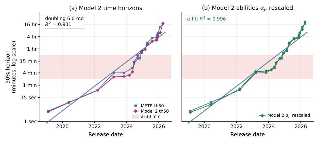
Figure 5(b) shows the results for Model 2, after an affine rescaling to compare it to the METR plot of Figure 1(a); Figure 5(a) overlays Model 2’s own time horizons on the same series, for reference. Strikingly, the rescaled abilities are almost identical to the METR estimates—visibly closer than Model 2’s own time horizons in panel (a). This means that even though the linear logistic model attempts to estimate time horizons, it may be inadvertently estimating another AI capability construct.
图 5(b) 展示了模型 2 的结果,经过仿射缩放后与图 1(a) 的 METR 图比较;作为参照,图 5(a) 把模型 2 自己的时间跨度叠加在同一序列上。引人注目的是,缩放后的能力与 METR 的估计几乎完全相同,比 (a) 中模型 2 自己的时间跨度明显更接近。这意味着,线性逻辑模型虽然试图估计时间跨度,实际上可能无意中估计了另一个 AI 能力构念。
Why does this coincidence occur? To be clear, it is not guaranteed to occur, and would not have occurred if the shape of the spline in Figure 1(d) diverged further from linear. In this case, note that under Model 2, the 50% log-time horizon can be defined as where , while in the linear model the log horizon is . So by plotting Model 2’s results without , the coincidence is that, up to rescaling, the estimates in each model are close to each other.
为什么会出现这种巧合?需要说明的是,它并不必然发生;如果图 1(d) 中样条的形状更偏离线性,就不会出现。在本例中,注意在模型 2 下,50% 对数时间跨度可以定义为 ,其中 ,而在线性模型中对数跨度为 。因此,不经 直接画出模型 2 的结果时,巧合在于:在相差一个缩放的意义下,两个模型中的估计 彼此接近。
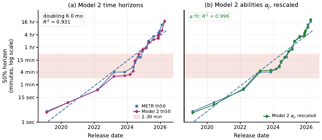
Figure 5: Model 2 over the METR plot. Both panels repeat METR’s own per-AI time horizons (blue, with the trend dashed), which are close to the baseline horizons of Figure 1(a). As in Figure 1, only frontier AIs are shown, each series on its own frontier. (a) Model 2’s time horizons (purple), the estimates of Figure 1(e); the disagreement concentrates in the shaded 2–30 minute band. (b) Model 2’s Rasch abilities (green), displayed as minutes with chosen by least squares against of the METR time horizons ().
图 5:把模型 2 叠加在 METR 图上。两个子图都重复给出 METR 自己的逐 AI 时间跨度(蓝色,趋势为虚线),它们与图 1(a) 的基线时间跨度很接近。与图 1 一样,图中只显示前沿 AI,每个序列各有自己的前沿。(a) 模型 2 的时间跨度(紫色),即图 1(e) 中的估计;分歧集中在阴影标出的 2–30 分钟区间。(b) 模型 2 的 Rasch 能力 (绿色),以 分钟显示,其中 通过对 METR 时间跨度的 做最小二乘选出()。
Because the flat region of is relatively localized to tasks within 2–30 min, while the estimation of and depends on ’s performance on every task, we believe that the linearity assumption on was close enough to correct on the whole task suite so that estimating still gave a good answer. However, if we believe that is truly not linear, we should not then call the estimate a time horizon, though we may still believe the measurements are nevertheless valuable as capturing Rasch ability.
由于 的平坦区域相对局限在 2–30 分钟的任务内,而 和 的估计取决于 在每一个任务上的表现,我们认为在整个任务套件上, 的线性假设已经足够接近正确,因此估计 仍然给出了不错的答案。然而,如果我们相信 确实不是线性的,就不应再把这个估计称为时间跨度,尽管我们仍可以认为这些测量值作为 Rasch 能力的刻画是有价值的。
4 Discussion: the future of time horizons
4 讨论:时间跨度的未来
It seems difficult to extend the time-horizon benchmark beyond the human time length of tasks that is currently available (up to 30 hours). However, suppose it were possible. Then there is no a priori reason that newly constructed, longer tasks should preserve the approximately linear relationship observed over the current range; future portions of may again be unusually flat or steep. It seems quite plausible that the estimated purple curve (and perhaps an underlying true pattern) could look like Figure 6, and checks on a linear model will not detect this, while our diagnostic plots will.
要把时间跨度基准扩展到超出现有任务的人类耗时长度(最长 30 小时),看起来很困难。但假设可以做到。那么,没有任何先验理由认为新构建的更长任务会保持当前范围内观察到的近似线性关系; 在未来的部分可能再次异常平坦或异常陡峭。估计出的紫色曲线(或许还有背后的真实规律)完全可能看起来像图 6 那样,而针对线性模型的检查发现不了这一点,我们的诊断图则可以。
Additionally, when assessing AI’s effects in the broader economy outside of software engineering, capability anchoring seems of great importance for scientific communication of the speed and risks of development. One domain with great opportunity is in physical intelligence, i.e. robotics. In this case, it seems of great importance to pick a good annotation to carefully assess the construct validity of time horizons to communicate advancement to the public. However, the best task annotation may not be human time.
此外,在评估 AI 对软件工程之外更广泛经济的影响时,能力锚定对于科学地传达 AI 发展的速度和风险显得非常重要。一个大有可为的领域是物理智能,即机器人。在这一领域,要向公众传达进展,挑选一个好的标注、仔细评估时间跨度的构念效度显得非常重要。不过,最好的任务标注未必是人类耗时。
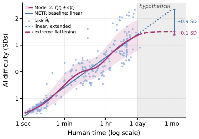
Figure 6: A hypothetical time-to-difficulty conversion beyond one day. Up to one day, the plot is Figure 1(d); after that, we depict a possible future for the time-to-difficulty conversion.
图 6:一天以上的假想耗时—难度换算。一天以内的部分即图 1(d);一天以后,我们描绘了耗时—难度换算的一种可能前景。
Acknowledgments and Disclosure of Funding
致谢与资助声明
We thank Alexander Barry, Miles Tidmarsh, Jonathan Gabor, and the AI safety community for useful discussions.
感谢 Alexander Barry、Miles Tidmarsh、Jonathan Gabor 以及 AI 安全社区的有益讨论。
References
参考文献
Baker [2001] Frank B. Baker. The Basics of Item Response Theory . ERIC Clearinghouse on Assessment and Evaluation, College Park, Md., 2nd ed edition, 2001. ISBN 978-1-886047-03-7.
Barry [2026] Alexander Barry. Impact of modelling assumptions on time horizon results. METR Blog , March 2026.
Dimitriadis et al. [2023] Timo Dimitriadis, Tilmann Gneiting, Alexander I. Jordan, and Peter Vogel. Evaluating Probabilistic Classifiers: The Triptych, January 2023.
Ehm et al. [2016] Werner Ehm, Tilmann Gneiting, Alexander Jordan, and Fabian Krüger. Of quantiles and expectiles: Consistent scoring functions, Choquet representations and forecast rankings. Journal of the Royal Statistical Society: Series B (Statistical Methodology) , 78(3):505–562, 2016.
Gregory Lewis [2026] Gregory Lewis. General capability - and capabilities generally - have no good y-axis, August 2026.
Ho et al. [2025] Anson Ho, Jean-Stanislas Denain, David Atanasov, Samuel Albanie, and Rohin Shah. A Rosetta Stone for AI Benchmarks, November 2025.
Kokotajlo et al. [2025] Daniel Kokotajlo, Scott Alexander, Thomas Larsen, Eli Lifland, and Romeo Dean. AI 2027. https://ai-2027.com/, April 2025.
Kwa [2026] Thomas Kwa. Clarifying limitations of time horizon. METR Blog , January 2026.
Kwa and Cheng [2025] Thomas Kwa and Vincent Cheng. How Does Time Horizon Vary Across Domains? METR Blog , July 2025.
Kwa et al. [2025] Thomas Kwa, Ben West, Joel Becker, Amy Deng, Katharyn Garcia, Max Hasin, Sami Jawhar, Megan Kinniment, Nate Rush, Sydney Von Arx, Ryan Bloom, Thomas Broadley, Haoxing Du, Brian Goodrich, Nikola Jurkovic, Luke Harold Miles, Seraphina Nix, Tao Roa Lin, Neev Parikh, David Rein, Lucas Jun Koba Sato, Hjalmar Wijk, Daniel M. Ziegler, Elizabeth Barnes, and Lawrence Chan. Measuring AI Ability to Complete Long Software Tasks. In The Thirty-ninth Annual Conference on Neural Information Processing Systems , October 2025.
Kwa et al. [2026] Thomas Kwa, Ben West, Joel Becker, Amy Deng, Katharyn Garcia, Max Hasin, Sami Jawhar, Megan Kinniment, Nate Rush, Sydney Von Arx, Ryan Bloom, Thomas Broadley, Haoxing Du, Brian Goodrich, Nikola Jurkovic, Luke Harold Miles, Seraphina Nix, Tao Lin, Neev Parikh, David Rein, Lucas Jun Koba Sato, Hjalmar Wijk, Daniel M. Ziegler, Elizabeth Barnes, and Lawrence Chan. Measuring AI Ability to Complete Long Software Tasks, February 2026.
Mertens et al. [2026] Matthias Mertens, Adam Kuzee, Brittany S. Harris, Harry Lyu, Wensu Li, Jonathan Rosenfeld, Meiri Anto, Martin Fleming, and Neil Thompson. Crashing Waves vs. Rising Tides: Preliminary Findings on AI Automation from Thousands of Worker Evaluations of Labor Market Tasks, April 2026.
Moss [2026] Jonas Moss. (Updated) METR’s data can’t distinguish between trajectories (and 80% horizons are an order of magnitude off). LessWrong, February 2026.
Narayanan and Kapoor [2025] Arvind Narayanan and Sayash Kapoor. AI as Normal Technology. http://knightcolumbia.org/content/ai-as-normal-technology, April 2025.
Roose [2026] Kevin Roose. How Do You Measure an A.I. Boom? The New York Times , April 2026. ISSN 0362-4331.
Schervish [1989] Mark J. Schervish. A general method for comparing probability assessors. The Annals of Statistics , 17(4):1856–1879, 1989.
shash42 [2025] shash42. How to game the METR plot. LessWrong, December 2025.
Steinhardt [2026] Jacob Steinhardt. Building Technology to Drive AI Governance. https://bounded-regret.ghost.io/building-technology-to-drive-ai-governance/, February 2026.
Stenner [2023] A. Jackson Stenner. Measuring Reading Comprehension with the Lexile Framework. In William P. Fisher Jr. and Paula J. Massengill, editors, Explanatory Models, Unit Standards, and Personalized Learning in Educational Measurement: Selected Papers by A. Jackson Stenner , pages 63–88. Springer Nature, Singapore, 2023. ISBN 978-981-19-3747-7. doi: 10.1007/978-981-19-3747-7_6 .
Witkin [2026] Nathan Witkin. Against the METR Graph, January 2026.
Witt [2025] Stephen Witt. Opinion | The A.I. Prompt That Could End the World. The New York Times , October 2025. ISSN 0362-4331.
Appendix A Appendix
附录 A 附录
A.1 Per-AI evaluations
A.1 逐 AI 评估
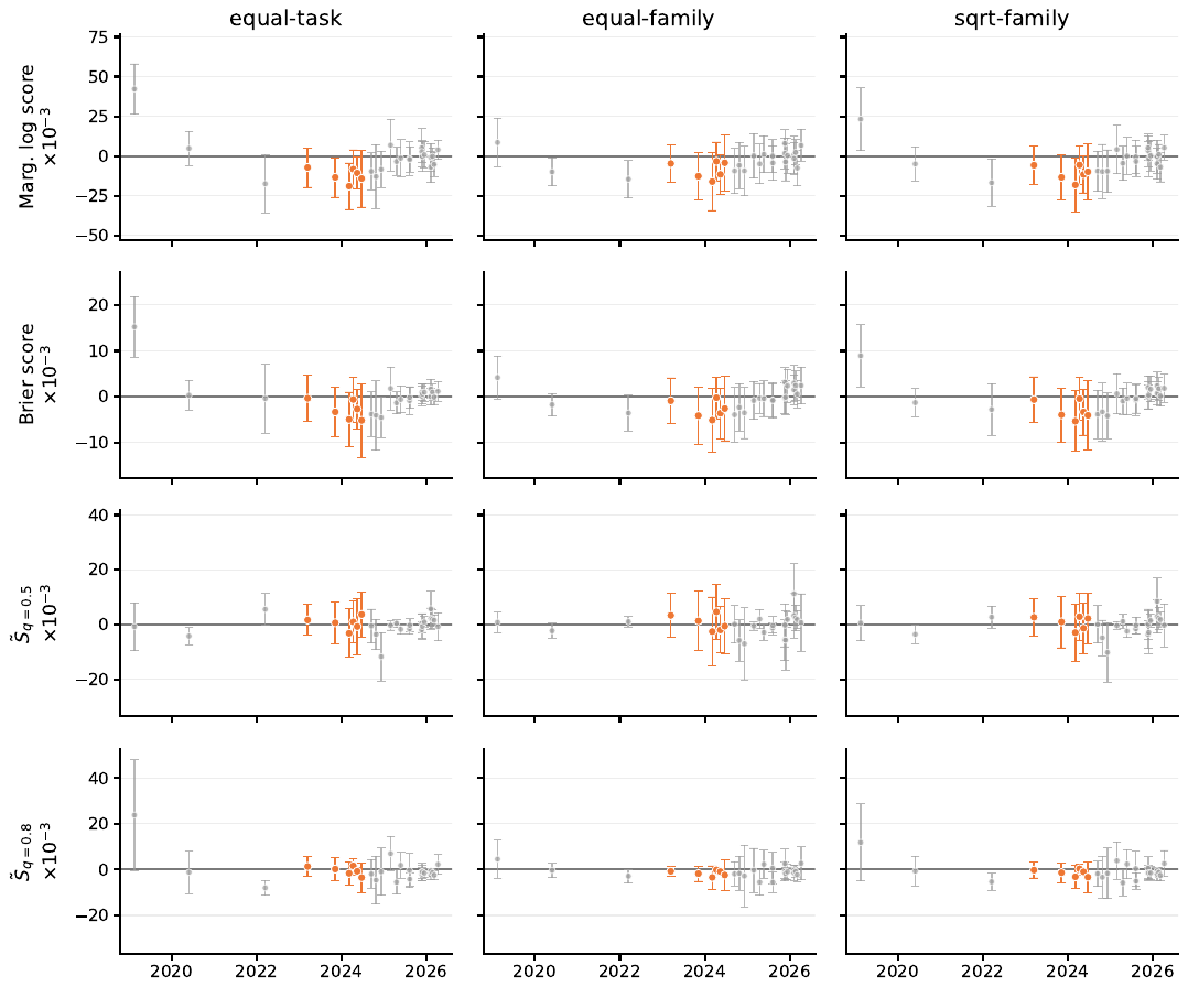
Figure 7: Per-AI scoring-rule contrasts, Model 1 baseline, for all 26 AIs in release order under family CV. Each point is the paired difference on that AI’s held-out cells (; below zero favors Model 1), with a 95% Bayle cluster-robust interval using the task families that AI attempted as clusters. Weights and family sizes are renormalized within each AI. Columns give the three evaluation weightings and rows the marginal log score, Brier score, and the smoothed elementary scores and , which average over and , respectively. Orange marks the six AIs of Figure 4, whose METR time horizons are 2–15 min; all other AIs are gray.
图 7:在任务族交叉验证下,全部 26 个 AI 按发布顺序排列的逐 AI 评分规则对比(模型 1 基线)。每个点是该 AI 留出单元上的配对差值(;低于零表示模型 1 更好),并给出 95% Bayle 聚类稳健区间,以该 AI 尝试过的任务族为聚类。权重和任务族大小在每个 AI 内部重新归一化。各列为三种评估加权,各行为边际对数分数、Brier 分数,以及平滑基本分数 和 ,二者分别在 和 上取平均。橙色标出图 4 中的六个 AI,它们的 METR 时间跨度为 2–15 分钟;其余 AI 为灰色。
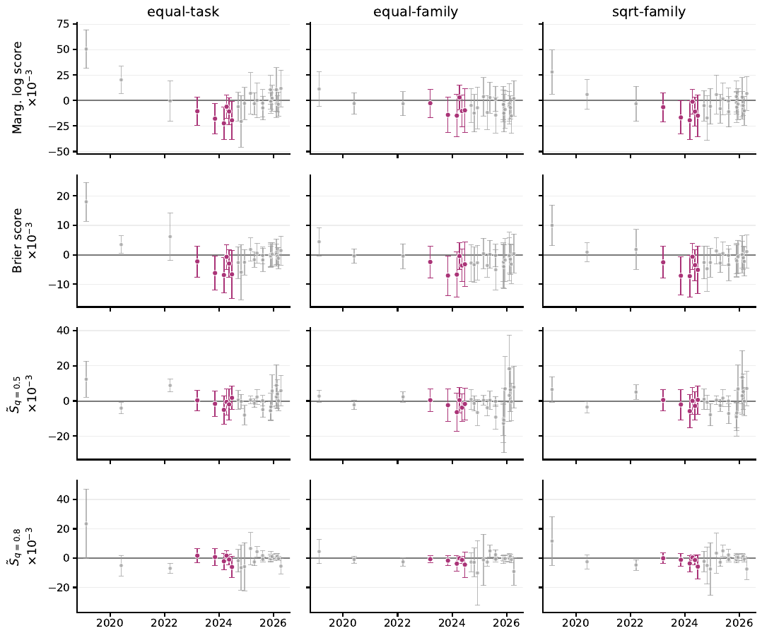
Figure 8: Per-AI scoring-rule contrasts, Model 2 baseline, with the same construction and shared score-wise axis limits as Figure 7. Purple marks the same six AIs with time horizons of 2–15 min. The point-estimate advantage is concentrated in the middle of the capability range, while most individual-AI intervals remain too wide to separate from zero; the pooled comparison in Figure 2 is where the evidence accumulates.
图 8:逐 AI 评分规则对比(模型 2 基线),构造方式和各分数共用的坐标轴范围与图 7 相同。紫色标出同样的六个时间跨度为 2–15 分钟的 AI。点估计上的优势集中在能力范围的中段,而大多数单个 AI 的区间仍然太宽,无法与零区分开;证据是在图 2 的汇总比较中累积起来的。
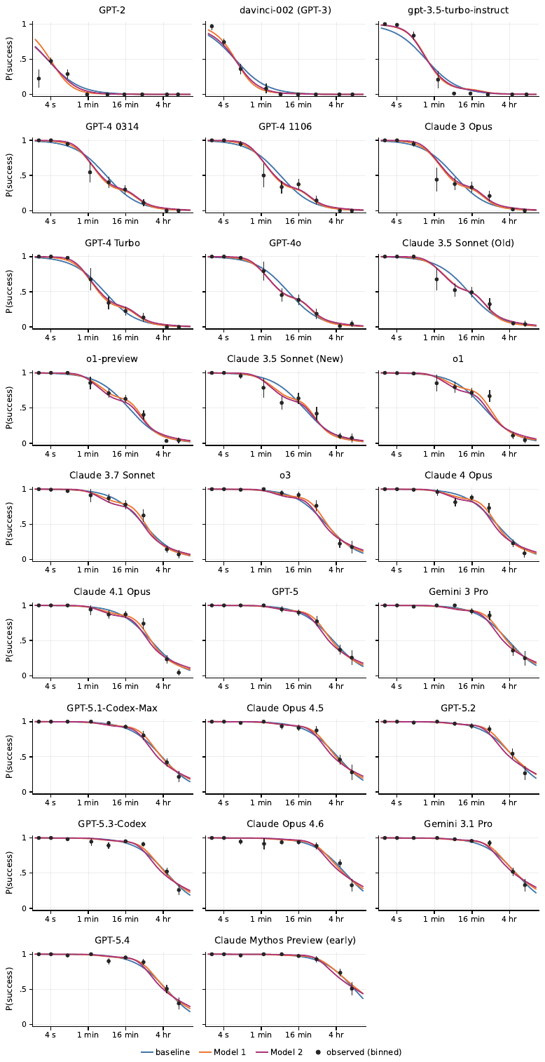
Figure 9: In-sample fitted against binned observed frequencies for all 26 AIs, in release order; construction as in Figure 4 (factor-4 human-time bins centered on 1 min, 4 min, 16 min, …; points at run-weighted mean human times, 95% Wald intervals treating runs as independent). The shape misfit of the log-linear baseline is concentrated in the mid-strength AIs of the GPT-4 era; for the weakest AIs the curves differ mainly in the tail, and for the strongest the three specifications nearly coincide.
图 9:全部 26 个 AI 按发布顺序排列的样本内拟合 与分箱观测频率对比,构造方式同图 4(以 1 分钟、4 分钟、16 分钟……为中心、按 4 倍间隔划分的人类耗时箱;点位于按运行次数加权的平均人类耗时处;95% Wald 区间把各次运行视为独立)。对数线性基线的形状失配集中在 GPT-4 时代的中等能力 AI 上;对最弱的 AI,各曲线主要在尾部不同;对最强的 AI,三种设定几乎重合。