MelGAN: Generative Adversarial Networks for Conditional Waveform Synthesis

MelGAN：面向条件波形合成的生成对抗网络

Kundan Kumar † † thanks: Equal contribution Affiliation:  Lyrebird AI, Mila, University of Montreal Email:  kundan@descript.com    Rithesh Kumar 1 1 footnotemark: 1 Affiliation:  Lyrebird AI Email:  rithesh@descript.com    Thibault de Boissiere Affiliation:  Lyrebird AI    Lucas Gestin Affiliation:  Lyrebird AI    Wei Zhen Teoh Affiliation:  Lyrebird AI    Jose Sotelo Affiliation:  Lyrebird AI, Mila    Alexandre de Brebisson Affiliation:  Lyrebird AI, Mila    Yoshua Bengio Affiliation:  Mila Affiliation:  University of Montreal, CIFAR Program Co-director    Aaron Courville Affiliation:  Mila Affiliation:  University of Montreal, CIFAR Fellow

Abstract

摘要

Previous works (Donahue et al., 2018a; Engel et al., 2019a) have found that generating coherent raw audio waveforms with GANs is challenging. In this paper, we show that it is possible to train GANs reliably to generate high quality coherent waveforms by introducing a set of architectural changes and simple training techniques. Subjective evaluation metric (Mean Opinion Score, or MOS) shows the effectiveness of the proposed approach for high quality mel-spectrogram inversion. To establish the generality of the proposed techniques, we show qualitative results of our model in speech synthesis, music domain translation and unconditional music synthesis. We evaluate the various components of the model through ablation studies and suggest a set of guidelines to design general purpose discriminators and generators for conditional sequence synthesis tasks. Our model is non-autoregressive, fully convolutional, with significantly fewer parameters than competing models and generalizes to unseen speakers for mel-spectrogram inversion. Our pytorch implementation runs at more than 100x faster than realtime on GTX 1080Ti GPU and more than 2x faster than real-time on CPU, without any hardware specific optimization tricks.

先前工作（Donahue et al., 2018a；Engel et al., 2019a）发现，用 GAN 生成连贯的原始音频波形并不容易。本文表明，通过一组结构改动与简单训练技巧，可以稳定训练 GAN 并生成高质量、连贯的波形。主观评测（平均意见分，MOS）显示，该方法在高质量梅尔频谱图反演上有效。为验证技术的通用性，我们还给出语音合成、音乐域翻译与无条件音乐合成上的定性结果。消融实验评估了各组件，并提出面向条件序列合成任务设计通用判别器与生成器的一组准则。模型为非自回归、全卷积，参数量明显少于竞争方法，且在梅尔频谱图反演上能泛化到未见过的说话人。我们的 PyTorch 实现在 GTX 1080Ti GPU 上超过实时 100 倍，在 CPU 上超过实时 2 倍，且未使用任何面向特定硬件的优化技巧。

1 Introduction

1 引言

Modelling raw audio is a particularly challenging problem because of the high temporal resolution of the data (usually atleast 16,000 samples per second) and the presence of structure at different timescales with short and long-term dependencies. Thus, instead of modelling the raw temporal audio directly, most approaches simplify the problem by modelling a lower-resolution representation that can be efficiently computed from the raw temporal signal. Such a representation is typically chosen to be easier to model than raw audio while preserving enough information to allow faithful inversion back to audio. In the case of speech, aligned linguistic features (Van Den Oord et al., 2016) and mel-spectograms (Shen et al., 2018; Gibiansky et al., 2017) are two commonly used intermediate representations. Audio modelling is thus typically decomposed into two stages. The first models the intermediate representation given text as input. The second transforms the intermediate representation back to audio. In this work, we focus on the latter stage, and choose mel-spectogram as the intermediate representation.[^1] Current approaches to mel-spectogram inversion can be categorized into three distinct families: pure signal processing techniques, autoregressive and non-autoregressive neural networks. We describe these three main lines of research in the following paragraphs.

原始音频建模特别难，因为时间分辨率很高（通常至少每秒 16,000 个采样），并且在不同时间尺度上都有结构，既有短程也有长程依赖。因此，多数方法并不直接对原始时间域音频建模，而是改用可从原始信号高效算出的低分辨率表示。这类表示通常比原始音频更容易建模，同时仍保留足以忠实反演回音频的信息。对语音而言，与原始音频时间对齐的语言学特征（Van Den Oord et al., 2016）以及梅尔频谱图（Shen et al., 2018；Gibiansky et al., 2017）是两类常用中间表示。音频建模因此常拆成两阶段：第一阶段以文本为输入建模中间表示；第二阶段把中间表示还原为音频。本文聚焦后一阶段，并选用梅尔频谱图作为中间表示。[^1] 当前梅尔频谱图反演大致分三族：纯信号处理、自回归神经网络与非自回归神经网络。下文分别介绍这三条主线。

Pure signal processing approaches

Different signal processing approaches have been explored to find some convenient low-resolution audio representations that can both be easily modelled and efficiently converted back to temporal audio. For example, the Griffin-Lim (Griffin & Lim, 1984) algorithm allows one to efficiently decode an STFT sequence back to the temporal signal at the cost of introducing strong, robotic artifacts as noted in Wang et al. (2017). More sophisticated representations and signal processing techniques have been investigated. For instance, the WORLD vocoder (MORISE et al., 2016) introduces an intermediate representation tailored to speech modelling based on mel-spectrogram-like features. The WORLD vocoder is paired with a dedicated signal processing algorithm to map the intermediate representation back to the original audio. It has been successfully used to carry out text-to-speech synthesis, for example in Char2Wav, where WORLD vocoder features are modelled with an attention-based recurrent neural network (Sotelo et al., 2017; Shen et al., 2018; Ping et al., 2017). The main issue with these pure signal processing methods is that the mapping from intermediate features to audio usually introduces noticeable artifacts.

纯信号处理方法

人们探索过多种信号处理路径，希望找到既易于建模又能高效还原时间域音频的低分辨率表示。例如 Griffin-Lim（Griffin & Lim, 1984）能高效把 STFT 序列解码回时间信号，但如 Wang et al.（2017）所指出，会引入明显的机器人般伪影。更精细的表示与算法也被研究过：WORLD 声码器（MORISE et al., 2016）引入面向语音建模、类似梅尔频谱的中间特征，并配以专用算法映射回原始音频；它曾成功用于文本到语音，例如 Char2Wav 用基于注意力的循环网络去建模 WORLD 特征（Sotelo et al., 2017；Shen et al., 2018；Ping et al., 2017）。这类纯信号处理方法的主要问题是：从中间特征到音频的映射通常会留下可察觉的伪影。

Autoregressive neural-networks-based models

WaveNet (Van Den Oord et al., 2016) is a fully-convolutional autoregressive sequence model that produces highly realistic speech samples conditioned on linguistic features that are temporally aligned with the raw audio. It is also capable of generating high quality unconditional speech and music samples. SampleRNN (Mehri et al., 2016) is an alternative architecture to perform unconditional waveform generation which explicitly models raw audio at different temporal resolutions using multi-scale recurrent neural networks. WaveRNN (Kalchbrenner et al., 2018) is a faster auto-regressive model based on a simple, single-layer recurrent neural network. WaveRNN introduces various techniques, such as sparsification and subscale generations to further increase synthesis speed. These methods have produced state-of-the-art results in text-to-speech synthesis (Sotelo et al., 2017; Shen et al., 2018; Ping et al., 2017) and other audio generation tasks (Engel et al., 2017). Unfortunately, inference with these models is inherently slow and inefficient because audio samples must be generated sequentially. Thus auto-regressive models are usually not suited for real-time applications.

基于自回归神经网络的模型

WaveNet（Van Den Oord et al., 2016）是全卷积自回归序列模型，在与原始音频时间对齐的语言学特征条件下，能生成高度逼真的语音样本，也能做高质量的无条件语音与音乐生成。SampleRNN（Mehri et al., 2016）用多尺度循环网络在不同时间分辨率上显式建模原始音频，是无条件波形生成的另一类结构。WaveRNN（Kalchbrenner et al., 2018）基于简单的单层循环网络，是更快的自回归方案，并引入稀疏化与子尺度生成等技巧以进一步提高合成速度。这些方法在文本到语音（Sotelo et al., 2017；Shen et al., 2018；Ping et al., 2017）及其他音频生成任务（Engel et al., 2017）上取得了当时最优结果。遗憾的是，推理本质上必须按采样点顺序生成，既慢又低效，因而自回归模型通常不适合实时应用。

Non autoregressive models

Recently, significant efforts have been dedicated to the development of non-autoregressive models to invert low-resolution audio representations. These models are orders of magnitudes faster than their auto-regressive counterparts because they are highly parallelizable and can fully exploit modern deep learning hardware (such as GPUs and TPUs). Two distinct methods have emerged to train such models. 1.) Parallel Wavenet (Oord et al., 2017) and Clarinet (Ping et al., 2018) distill a trained auto-regressive decoder into a flow-based convolutional student model. The student is trained using a probability distillation objective based on the Kulback-Leibler divergence: $KL[P_{\text{student}}||P_{\text{teacher}}]$, along with an additional perceptual loss terms. 2.) WaveGlow (Prenger et al., 2019) is a flow-based generative model based on Glow (Kingma & Dhariwal, 2018). WaveGlow is a very high capacity generative flow consisting of 12 coupling and 12 invertible 1x1 convolutions, with each coupling layer consisting of a stack of 8 layers of dilated convolutions. The authors note that it requires a week of training on 8 GPUs to get good quality results for a single speaker model. While inference is fast on the GPU, the large size of the model makes it impractical for applications with a constrained memory budget.

非自回归模型

近来大量工作转向用非自回归模型反演低分辨率音频表示。它们高度可并行，能充分利用 GPU、TPU 等硬件，速度比自回归方法高出几个数量级。训练此类模型主要有两条路。1）Parallel WaveNet（Oord et al., 2017）与 Clarinet（Ping et al., 2018）把已训练的自回归解码器蒸馏到基于流的卷积学生模型中；学生用基于 Kullback–Leibler 散度的概率蒸馏目标 $KL[P_{\text{student}}||P_{\text{teacher}}]$，再加感知损失项。2）WaveGlow（Prenger et al., 2019）是基于 Glow（Kingma & Dhariwal, 2018）的流生成模型，容量很大：12 个耦合层与 12 个可逆 1×1 卷积，每个耦合层又是 8 层膨胀卷积的堆叠。作者指出，单说话人模型要在 8 块 GPU 上训练约一周才有不错音质。GPU 上推理虽快，但模型体量使其在内存受限场景中不便使用。

GANs for audio

One family of methods that has so far been little explored for audio modelling are generative adversarial networks (GANs) (Goodfellow et al., 2014). GANs have made steady progress in unconditional image generation (Gulrajani et al., 2017; Karras et al., 2017; Karras et al., 2018), image-to-image translation (Isola et al., 2017; Zhu et al., 2017; Wang et al., 2018b) and video-to-video synthesis (Chan et al., 2018; Wang et al., 2018a). Despite their huge success in computer vision, we have not seen as much progress in using GANs for audio modelling. Engel et al. (2019b) use GANs to generate musical timbre by modelling STFT magnitudes and phase angles instead of modelling raw waveform directly. Neekhara et al. (2019) propose using GANs to learn mappings from mel-spectrogram to simple magnitude spectrogram, which is to be combined with phase estimations to recover raw audio waveform. Yamamoto et al. (2019) use GANs to distill an autoregressive model that generates raw speech audio, however their results show that adversarial loss alone is not sufficient for high quality waveform generation; it requires a KL-divergence based distillation objective as a critical component. To this date, making them work well in this domain has been challenging (Donahue et al., 2018a).

面向音频的 GAN

迄今在音频建模中探索较少的一族方法是生成对抗网络（GAN）（Goodfellow et al., 2014）。GAN 在无条件图像生成（Gulrajani et al., 2017；Karras et al., 2017；Karras et al., 2018）、图像到图像翻译（Isola et al., 2017；Zhu et al., 2017；Wang et al., 2018b）以及视频到视频合成（Chan et al., 2018；Wang et al., 2018a）上稳步推进。尽管在计算机视觉中极为成功，音频建模上的进展却远不及此。Engel et al.（2019b）用 GAN 生成音乐音色时建模的是 STFT 幅度与相位角，而非直接建模原始波形。Neekhara et al.（2019）提出用 GAN 学习从梅尔频谱到简单幅度谱的映射，再结合相位估计恢复原始波形。Yamamoto et al.（2019）用 GAN 蒸馏生成原始语音的自回归模型，但其结果表明：仅靠对抗损失不足以得到高质量波形，基于 KL 散度的蒸馏目标仍是关键组件。时至今日，让 GAN 在该领域稳定好用仍很困难（Donahue et al., 2018a）。

Main Contributions

• • We introduce MelGAN, a non-autoregressive feed-forward convolutional architecture to perform audio waveform generation in a GAN setup. To the best of our knowledge, this is the first work that successfully trains GANs for raw audio generation without additional distillation or perceptual loss functions while still yielding a high quality text-to-speech synthesis model.

主要贡献

• • 我们提出 MelGAN：在 GAN 设定下做音频波形生成的非自回归前馈卷积结构。据我们所知，这是首个在无需额外蒸馏或感知损失的情况下，成功训练 GAN 做原始音频生成、并能支撑高质量文本到语音合成的工作。

• • We show that autoregressive models can be readily replaced with a fast and parallel MelGAN decoder for raw waveform generation through experiments in universal music translation, text-to-speech generation and unconditional music synthesis albeit with slight quality degradation.

• • 通过通用音乐翻译、文本到语音生成与无条件音乐合成等实验，我们表明可用快速、并行的 MelGAN 解码器替换自回归模型来生成原始波形，音质仅略有下降。

• • We also show that MelGAN is substantially faster than other mel-spectrogram inversion alternatives. In particular, it is 10 times faster than the fastest available model to date (Prenger et al., 2019) without considerable degradation in audio quality.

• • 我们还表明 MelGAN 明显快于其他梅尔频谱图反演方案。具体而言，相对当时最快可用模型（Prenger et al., 2019）约快 10 倍，且音质没有明显下降。

2 The MelGAN Model

2 MelGAN 模型

In this section, we describe our generator and discriminator architectures for mel-spectrogram inversion. We describe the core components of the model and discuss modifications to perform unconditional audio synthesis. We compare the proposed model with competing approaches in terms of number of parameters and inference speed on both CPU and GPU. Figure 1 shows the overall architecture.

本节描述用于梅尔频谱图反演的生成器与判别器结构，说明模型核心组件，并讨论如何改造成无条件音频合成。我们还在参数量以及 CPU、GPU 推理速度上与竞争方法对比。整体结构见图 1。

(a) Generator

（a）生成器

2.1 Generator

2.1 生成器

Architecture

Our generator is a fully convolutional feed-forward network with mel-spectrogram $s$ as input and raw waveform $x$ as output. Since the mel-spectrogram (used for all experiments) is at a 256$\times$ lower temporal resolution, we use a stack of transposed convolutional layers to upsample the input sequence. Each transposed convolutional layer is followed by a stack of residual blocks with dilated convolutions. Unlike traditional GANs, our generator does not use a global noise vector as input. We noticed in our experiments that there is little perceptual difference in the generated waveforms when additional noise is fed to the generator. This is a counter-intuitive result because the inversion of $s\rightarrow x$ involves a one-to-many mapping since $s$ is a lossy-compression of $x$. However, this finding is consistent with Mathieu et al. (2015) and Isola et al. (2017), which show that noise input is not important if the conditioning information is very strong.

结构

生成器是全卷积前馈网络，输入为梅尔频谱图 $s$，输出为原始波形 $x$。实验所用梅尔频谱图在时间上低了 256 倍，因此用一叠转置卷积做上采样；每层转置卷积后再接带膨胀卷积的残差块堆叠。与传统 GAN 不同，我们的生成器不以全局噪声向量为输入。实验中发现：额外喂噪声时，生成波形的感知差异很小。这一结果有些反直觉，因为 $s\rightarrow x$ 是一对多映射（$s$ 是 $x$ 的有损压缩）。不过这与 Mathieu et al.（2015）与 Isola et al.（2017）一致：当条件信息足够强时，噪声输入并不重要。

Induced receptive field

In convolutional neural network based generators for images, there is an inductive bias that pixels which are spatially close-by are correlated because of high overlap among their induced receptive fields. We design our generator architecture to put an inductive bias that there is long range correlation among the audio timesteps. We added residual blocks with dilations after each upsampling layer, so that temporally far output activations of each subsequent layer has significant overlapping inputs. Receptive field of a stack of dilated convolution layers increases exponentially with the number of layers. Similar to Van Den Oord et al. (2016), incorporating these in our generator allows us to efficiently increase the induced receptive fields of each output time-step. This effectively implies larger overlap in the induced receptive field of far apart time-steps, leading to better long range correlation.

诱导感受野

在面向图像的卷积生成器中，空间相近的像素因诱导感受野高度重叠而相关，这是一种归纳偏置。我们设计生成器时，则希望在音频时间步之间引入长程相关的归纳偏置：在每个上采样层后加入带膨胀的残差块，使后续层时间上相距较远的输出激活仍有显著重叠输入。膨胀卷积堆叠的感受野随层数指数增长。与 Van Den Oord et al.（2016）类似，把它们放进生成器可高效扩大每个输出时间步的诱导感受野，从而使相距较远的时间步在感受野上有更大重叠，有利于长程相关。

Checkerboard artifacts

As noticed in Odena et al. (2016), deconvolutional generators are susceptible to generating "checkerboard" patterns if the kernel-size and stride of the transposed convolutional layers are not carefully chosen. Donahue et al. (2018b) examines this for raw waveform generation and finds that such repeated patterns lead to audible high frequency hissing noise. We solve this problem by carefully choosing the kernel-size and stride for our deconvolutional layers as a simpler alternative to PhaseShuffle layer introduced in Donahue et al. (2018b). Following Odena et al. (2016), we use kernel-size as a multiple of stride. Another source of such repeated patterns, can be the dilated convolution stack if dilation and kernel size are not chosen correctly. We make sure that the dilation grows as a power of the kernel-size such that the receptive field of the stack looks like a fully balanced (seeing input uniformly) and symmetric tree with kernel-size as the branching factor.

棋盘伪影

如 Odena et al.（2016）所指出，若转置卷积的核大小与步长选择不当，反卷积生成器容易产生「棋盘」图案。Donahue et al.（2018b）在原始波形生成中考察了这一问题，发现这类重复图案会造成可听见的高频嘶声。我们通过仔细选择反卷积层的核大小与步长来解决，作为相对 Donahue et al.（2018b）中 PhaseShuffle 层的更简单替代。遵循 Odena et al.（2016），核大小取为步长的整数倍。另一类重复图案可能来自膨胀卷积堆叠：若膨胀与核大小不匹配也会出问题。我们令膨胀按核大小的幂次增长，使堆叠的感受野像一棵以核大小为分支因子的、对输入均匀采样且对称的平衡树。

Normalization technique

We noticed that the choice of normalization technique for the generator was extremely crucial for sample quality. Popular conditional GAN architectures for image generation (Isola et al., 2017; Wang et al., 2018b) use instance normalization (Ulyanov et al., 2016) in all the layers of the generator. However, in the case of audio generation we found that instance normalization washes away important important pitch information, making the audio sound metallic. We also obtained poor results when applying spectral normalization (Miyato et al., 2018) on the generator as suggested in Zhang et al. (2018); Park et al. (2019). We believe that the strong Lipshitz constraint on the discriminator impacts the feature matching objective (explained in Section 3.2) used to train the generator. Weight normalization (Salimans & Kingma, 2016) worked best out of all the available normalization techniques since it does not limit the capacity of the discriminator or normalize the activations. It simply reparameterizes the weight matrices by decoupling the scale of the weight vector from the direction, to have better training dynamics. We therefore use weight normalization in all layers of the generator.

归一化技术

我们发现生成器的归一化选择对样本质量极为关键。流行的条件图像 GAN（Isola et al., 2017；Wang et al., 2018b）在生成器各层使用实例归一化（Ulyanov et al., 2016）。但在音频生成中，实例归一化会冲掉重要的音高信息，使声音发「金属感」。按 Zhang et al.（2018）；Park et al.（2019）的建议对生成器做谱归一化（Miyato et al., 2018）效果也很差。我们推测：对判别器过强的 Lipschitz 约束会干扰用于训练生成器的特征匹配目标（见第 3.2 节）。在所有可用归一化中，权重归一化（Salimans & Kingma, 2016）表现最好：它既不限制判别器容量，也不归一化激活，只是把权重矩阵重参数化为「尺度与方向解耦」，以改善训练动态。因此生成器各层一律使用权重归一化。

2.2 Discriminator

2.2 判别器

Multi-Scale Architecture

Following Wang et al. (2018b), we adopt a multi-scale architecture with 3 discriminators ($D_{1},D_{2},D_{3}$) that have identical network structure but operate on different audio scales. $D_{1}$ operates on the scale of raw audio, whereas $D_{2},D_{3}$ operate on raw audio downsampled by a factor of 2 and 4 respectively. The downsampling is performed using strided average pooling with kernel size 4. Multiple discriminators at different scales are motivated from the fact that audio has structure at different levels. This structure has an inductive bias that each discriminator learns features for different frequency range of the audio. For example, the discriminator operating on downsampled audio, does not have access to high frequency component, hence, it is biased to learn discriminative features based on low frequency components only.

多尺度结构

遵循 Wang et al.（2018b），我们采用多尺度结构：三个判别器（$D_{1},D_{2},D_{3}$）网络相同，但工作在不同音频尺度上。$D_{1}$ 作用于原始音频尺度，$D_{2},D_{3}$ 分别作用于下采样 2 倍与 4 倍后的原始音频；下采样用核大小为 4 的跨步平均池化。多尺度判别器的动机是：音频在不同层级都有结构，这一归纳偏置使各判别器学习不同频段上的特征。例如，作用于下采样音频的判别器接触不到高频成分，因而更偏向基于低频成分学习判别特征。

Window-based objective

Each individual discriminator is a Markovian window-based discriminator (analogues to image patches, Isola et al. (2017)) consisting of a sequence of strided convolutional layers with large kernel size. We utilize grouped convolutions to allow the use of larger kernel sizes while keeping number of parameters small. While a standard GAN discriminator learns to classify between distributions of entire audio sequences, window-based discriminator learns to classify between distribution of small audio chunks. Since the discriminator loss is computed over the overlapping windows where each window is very large (equal to the receptive field of the discriminator), the MelGAN model learns to maintain coherence across patches. We chose window-based discriminators since they have been shown to capture essential high frequency structure, require fewer parameters, run faster and can be applied to variable length audio sequences. Similar to the generator, we use weight normalization in all layers of the discriminator.

基于窗口的目标

每个判别器都是马尔可夫式、基于窗口的判别器（类比图像中的图块，Isola et al., 2017），由一串大核跨步卷积组成。我们用分组卷积，以便在参数量不大时使用更大的核。标准 GAN 判别器区分的是整段音频序列的分布，而基于窗口的判别器区分的是短音频块的分布。由于判别损失在重叠窗口上计算，且每个窗口很大（等于判别器感受野），MelGAN 能学会在图块之间保持连贯。选用窗口判别器是因为它们善于抓住必要的高频结构、参数更少、更快，且可作用于可变长度音频。与生成器一样，判别器各层也使用权重归一化。

2.3 Training objective

2.3 训练目标

To train the GAN, we use the hinge loss version of the GAN objective (Lim & Ye, 2017; Miyato et al., 2018). We also experimented with the least-squares (LSGAN) formulation (Mao et al., 2017) and noticed slight improvements with the hinge version.

训练 GAN 时我们采用 hinge 形式的对抗目标（Lim & Ye, 2017；Miyato et al., 2018）。我们也试过最小二乘（LSGAN）形式（Mao et al., 2017），发现 hinge 略好。

$$\displaystyle\min_{D_{k}}\mathbb{E}_{x}\Big[\min(0,1-D_{k}(x))\Big]+\mathbb{E}_{s,z}\Big[\min(0,1+D_{k}(G(s,z)))\Big],\ \forall k=1,2,3 \\ \displaystyle\min_{G}\mathbb{E}_{s,z}\Bigg[\sum_{k=1,2,3}-D_{k}(G(s,z))\Bigg] \tag{1}$$

where $x$ represents the raw waveform, $s$ represents the conditioning information (eg. mel-spectrogram) and $z$ represents the gaussian noise vector.

其中 $x$ 表示原始波形，$s$ 表示条件信息（例如梅尔频谱图），$z$ 表示高斯噪声向量。

Feature Matching

In addition to the discriminator’s signal, we use a feature matching objective (Larsen et al., 2015) to train the generator. This objective minimizes the L1 distance between the discriminator feature maps of real and synthetic audio. Intuitively, this can be seen as a learned similarity metric, where a discriminator learns a feature space that discriminates the fake data from real data. It is worth noting that we do not use any loss in the raw audio space. This is counter to other conditional GANs (Isola et al., 2017) where L1 loss is used to match conditionally generated images and their corresponding ground-truths, to enforce global coherence. In fact, in our case adding L1 loss in audio space introduces audible noise that hurts audio quality.

特征匹配

除判别器信号外，我们用特征匹配目标（Larsen et al., 2015）训练生成器：最小化真实与合成音频在判别器特征图上的 L1 距离。直观上，这可看成学到的相似度度量——判别器学出一个能区分真假数据的特征空间。需要说明：我们不在原始音频空间使用任何损失。这与其他条件 GAN（Isola et al., 2017）不同：后者常用 L1 去对齐条件生成图像与对应真值以强制全局连贯。事实上，在我们的设定下，在音频空间加 L1 会引入可听见噪声，反而伤害音质。

$$\displaystyle\mathcal{L}_{\text{FM}}(G,D_{k})=\mathbb{E}_{x,s\sim p_{\text{data}}}\Bigg[\sum_{i=1}^{T}\frac{1}{N_{i}}||D_{k}^{(i)}(x)-D_{k}^{(i)}(G(s))||_{1}\Bigg] \tag{3}$$

For simplicity of notation, $D_{k}^{(i)}$ represents the $i^{\text{th}}$ layer feature map output of the $k^{\text{th}}$ discriminator block, $N_{i}$ denotes the number of units in each layer. Feature matching is similar to the perceptual loss (Dosovitskiy & Brox, 2016; Gatys et al., 2016; Johnson et al., 2016). In our work, we use feature matching at each intermediate layer of all discriminator blocks.

为简化记号，$D_{k}^{(i)}$ 表示第 $k$ 个判别器块第 $i$ 层的特征图输出，$N_{i}$ 为该层单元数。特征匹配类似于感知损失（Dosovitskiy & Brox, 2016；Gatys et al., 2016；Johnson et al., 2016）。本文对所有判别器块的每一中间层都使用特征匹配。

We use the following final objective to train the generator, with $\lambda=10$ as in (Wang et al., 2018b):

训练生成器的最终目标如下，其中 $\lambda=10$，与 Wang et al.（2018b）一致：

$$\displaystyle\min_{G}\Bigg(\mathbb{E}_{s,z}\bigg[\sum_{k=1,2,3}-D_{k}(G(s,z))\bigg]+\lambda\sum_{k=1}^{3}\mathcal{L}_{\text{FM}}(G,D_{k})\Bigg) \tag{4}$$

2.4 Number of parameters and inference speed

2.4 参数量与推理速度

The inductive biases incorporated in our architecture make the overall model significantly smaller than competing models in terms of number of parameters. Being non-autoregressive and fully convolutional, our model is very fast at inference time, capable of running at a frequency of 2500kHz on GTX1080 Ti GPU in full precision (more than $10\times$ faster than the fastest competing model), and 50kHz on CPU (more than $25\times$ faster than the fastest competing model). We believe that our model is also well-suited for hardware specific inference optimization (such as half precision on Tesla V100 (Jia et al., 2018; Dosovitskiy & Brox, 2016) and quantization (as done in Arik et al. (2017)) which will further boost inference speed. Table 3 shows the detailed comparison.

结构中嵌入的归纳偏置使整体模型在参数量上显著小于竞争方法。由于非自回归且全卷积，推理很快：在 GTX 1080 Ti 上全精度可达约 2500 kHz（比当时最快竞争模型快 10 倍以上），在 CPU 上约 50 kHz（快 25 倍以上）。我们相信该模型也适合面向硬件的推理优化（例如 Tesla V100 半精度（Jia et al., 2018；Dosovitskiy & Brox, 2016）以及量化（如 Arik et al., 2017）），从而进一步提速。表 3 给出详细对比。

Model	Number of parameters (in millions)	Number of parameters	(in millions)	Speed on CPU (in kHz)	Speed on CPU	(in kHz)	Speed on GPU (in kHz)	Speed on GPU	(in kHz)
Number of parameters
(in millions)
Speed on CPU
(in kHz)
Speed on GPU
(in kHz)
Wavenet (Shen et al., 2018)	24.7	0.0627	0.0787
Clarinet (Ping et al., 2018)	10.0	1.96	221
WaveGlow (Prenger et al., 2019)	87.9	1.58	223
MelGAN (ours)	4.26	51.9	2500

Number of parameters
(in millions)

Speed on CPU
(in kHz)

Speed on GPU
(in kHz)

Table 1: Comparison of the number of parameters and the inference speed. Speed of $n$ kHz means that the model can generate $n\times 1000$ raw audio samples per second. All models are benchmarked using the same hardware [^3].

模型	参数量（百万）	CPU 速度（kHz）	GPU 速度（kHz）
Wavenet (Shen et al., 2018)	24.7	0.0627	0.0787
Clarinet (Ping et al., 2018)	10.0	1.96	221
WaveGlow (Prenger et al., 2019)	87.9	1.58	223
MelGAN（本文）	4.26	51.9	2500

表 1：参数量与推理速度对比。速度为 $n$ kHz 表示模型每秒可生成 $n\times 1000$ 个原始音频采样。所有模型在相同硬件上评测。[^3]

3 Results

3 结果

To encourage reproduciblity, we attach the code[^4] accompanying the paper.

为便于复现，我们附上与论文配套的代码。[^4]

3.1 Ground truth mel-spectrogram inversion

3.1 真值梅尔频谱图反演

Ablation study

First, in order to understand the importance of various components of our proposed model, we perform qualitative and quantitative analysis of the reconstructed audio for the mel-spectrogram inversion task. We remove certain key architectural decisions and evaluate the audio quality using the test set. Table 2 shows the mean opinion score of audio quality as assessed via human listening tests. Each model is trained for $400k$ iterations on the LJ Speech dataset (Ito, 2017). Our analysis leads to the following conclusions: Absence of dilated convolutional stacks in the generator or removing weight normalization lead to high frequency artifacts. Using a single discriminator (instead of multi-scale discriminator) produces metallic audio, especially while the speaker is breathing. Moreover, on our internal 6 clean speakers dataset, we notice that this version of the model skips certain voiced portions, completely missing some words. Using spectral normalization or removing the window-based discriminator loss makes it harder to learn sharp high frequency patterns, causing samples to sound significantly noisy. Adding an extra L1 penalty between real and generated raw waveform makes samples sound metallic with additional high frequency artifacts.

消融实验

首先，为理解所提模型各组件的重要性，我们对梅尔频谱图反演任务的重建音频做定性与定量分析：去掉若干关键结构选择，再在测试集上评估音质。表 2 给出经人工听音得到的平均意见分。每个模型在 LJ Speech（Ito, 2017）上训练 $400k$ 次迭代。分析得出如下结论：生成器中缺少膨胀卷积堆叠，或去掉权重归一化，都会带来高频伪影；使用单个判别器（而非多尺度）会使声音发金属感，尤其在说话人呼吸段；在我们内部的 6 名干净说话人数据上，该变体还会跳过某些浊音段、整词丢失。使用谱归一化或去掉基于窗口的判别损失，会使尖锐高频模式更难学，样本明显更噪。在真实与生成原始波形之间额外加 L1 惩罚，会使样本发金属感并伴随额外高频伪影。

Model	MOS	95% CI
w/ Spectral Normalization	1.33	$\pm$0.07
w/ L1 loss (audio space)	2.59	$\pm$0.11
w/o Window-based Discriminator	2.29	$\pm$0.10
w/o Dilated Convolutions	2.60	$\pm$0.10
w/o Multi-scale Discriminator	2.93	$\pm$0.11
w/o Weight Normalization	3.03	$\pm$0.10
Baseline (MelGAN)	3.09	$\pm$0.11

Table 2: Mean Opinion Score of ablation studies. To evaluate the biases induced by each component, we remove them one at a time, and train the model for 500 epochs each. Evaluation protocol/details can be found in appendix B.

模型	MOS	95% CI
加谱归一化	1.33	$\pm$0.07
加 L1 损失（音频空间）	2.59	$\pm$0.11
去掉基于窗口的判别器	2.29	$\pm$0.10
去掉膨胀卷积	2.60	$\pm$0.10
去掉多尺度判别器	2.93	$\pm$0.11
去掉权重归一化	3.03	$\pm$0.10
基线（MelGAN）	3.09	$\pm$0.11

表 2：消融实验的平均意见分。为评估各组件引入的偏置，我们每次去掉一个组件，各训练 500 个 epoch。评测协议见附录 B。

Benchmarking competing models

Model	MOS	95% CI
Griffin Lim	1.57	$\pm$0.04
WaveGlow	4.11	$\pm$0.05
WaveNet	4.05	$\pm$0.05
MelGAN	3.61	$\pm$0.06
Original	4.52	$\pm$0.04

Table 3: Mean Opinion Scores

与竞争模型对比

模型	MOS	95% CI
Griffin Lim	1.57	$\pm$0.04
WaveGlow	4.11	$\pm$0.05
WaveNet	4.05	$\pm$0.05
MelGAN	3.61	$\pm$0.06
原始音频	4.52	$\pm$0.04

表 3：平均意见分

Next, in order to compare the performance of MelGAN for inverting ground truth mel-spectrograms to raw audio against existing methods such as WaveNet vocoder, WaveGlow, Griffin-Lim and Ground Truth audio, we run an independent MOS test where the MelGAN model is trained until convergence (around $2.5M$ iterations). Similar to the ablation study, these comparisons are made on models trained on the LJ Speech Datset. The results of this comparison are shown in Table 3.

接下来，为把 MelGAN 在「真值梅尔频谱 → 原始音频」上的表现与 WaveNet 声码器、WaveGlow、Griffin-Lim 以及真值音频对比，我们另跑一轮 MOS 测试；MelGAN 训练至收敛（约 $2.5M$ 次迭代）。与消融相同，这些对比均基于在 LJ Speech 上训练的模型。结果见表 3。

This experiment result indicates that MelGAN is comparable in quality to state-of-the-art high capacity WaveNet-based models such as WaveNet and WaveGlow. We believe that the performance gap can be quickly bridged in the future by further exploring this direction of using GANs for audio synthesis.

该实验表明 MelGAN 在音质上可与 WaveNet、WaveGlow 等高容量、基于 WaveNet 的模型相比。我们相信，继续沿 GAN 音频合成方向探索，性能差距有望较快缩小。

Model	MOS	95% CI
Griffin Lim	1.72	$\pm$0.07
MelGAN	3.49	$\pm$0.09
Original	4.19	$\pm$0.08

Table 4: Mean Opinion Scores on the VCTK dataset (Veaux et al., 2017).

模型	MOS	95% CI
Griffin Lim	1.72	$\pm$0.07
MelGAN	3.49	$\pm$0.09
原始音频	4.19	$\pm$0.08

表 4：VCTK 数据集（Veaux et al., 2017）上的平均意见分。

Generalization to unseen speakers

Interestingly, we noticed that when we train MelGAN on a dataset containing multiple speakers (internal 6 speaker dataset consisting of 3 male and 3 female speakers with roughly 10 hours per speaker), the resulting model is able to generalize to completely new (unseen) speakers outside the train set. This experiment verifies that MelGAN is able to learn a speaker-invariant mapping of mel spectrograms to raw waveforms.

泛化到未见说话人

有意思的是，当我们在包含多名说话人的数据（内部 6 人集：3 男 3 女，每人约 10 小时）上训练 MelGAN 时，得到的模型能泛化到训练集之外的全新说话人。这说明 MelGAN 学到的是说话人无关的「梅尔频谱 → 原始波形」映射。

In an attempt to provide an easily comparable metric to systematically evaluate this generalization (for current and future work), we run an MOS hearing test for ground-truth mel-spectrogram inversion on the public available VCTK dataset (Veaux et al., 2017). The results of this test are shown in Table 4.

为给当前与后续工作提供便于系统对比的指标，我们在公开的 VCTK（Veaux et al., 2017）上对真值梅尔频谱反演做了 MOS 听音测试。结果见表 4。

3.2 End-to-end speech synthesis

3.2 端到端语音合成

Figure 2: Text-to-speech pipeline.

图 2：文本到语音流水线。

We perform quantitative and qualitative comparisons between our proposed MelGAN vs competing models on mel-spectrogram inversion for end-to-end speech synthesis. We plug the MelGAN model in an end-to-end speech synthesis pipeline (Figure 2) and evaluate the text-to-speech sample quality with competing models.

我们在端到端语音合成的梅尔频谱反演上，对 MelGAN 与竞争模型做定量与定性对比：把 MelGAN 接入端到端语音合成流水线（图 2），并与竞争模型一起评估文本到语音样本的质量。

Specifically, we compare the sample quality when using MelGAN for spectrogram inversion vs WaveGlow using Text2mel - an improved version of the open-source char2wav model (Sotelo et al., 2017). Text2mel generates mel-spectrograms instead of vocoder frames, uses phonemes as the input representation and can be coupled with WaveGlow or MelGAN to invert the generated mel-spectrograms. We use this model since its sampler, trains faster and does not perform any mel-frequency clipping like Tacotron2. Additionally, we also include the state-of-the-art Tacotron2 model (Shen et al., 2018) coupled with WaveGlow for baseline comparison. We use the open source implementations of Tacotron2 and WaveGlow provided by NVIDIA in the Pytorch Hub repository to generate the samples. When using WaveGlow, we use the Denoiser with strength $0.01$ provided in the official repository to remove high frequency artifacts. The results of the MOS tests are shown in the table 5.

具体而言，我们比较用 MelGAN 与用 WaveGlow 做频谱反演时的样本质量，前端是 Text2mel——开源 char2wav（Sotelo et al., 2017）的改进版。Text2mel 生成的是梅尔频谱而非声码器帧，输入为音素表示，可与 WaveGlow 或 MelGAN 耦合以反演生成的梅尔频谱。选用它是因为采样器训练更快，且不像 Tacotron2 那样对梅尔频率做裁剪。我们还纳入当时最优的 Tacotron2（Shen et al., 2018）+ WaveGlow 作为基线；样本由 NVIDIA 在 Pytorch Hub 上提供的 Tacotron2 与 WaveGlow 开源实现生成。使用 WaveGlow 时，按官方仓库提供的 Denoiser、强度 $0.01$ 去除高频伪影。MOS 结果见表 5。

Model	MOS	95% CI
Tacotron2 + WaveGlow	3.52	$\pm$0.04
Text2mel + WaveGlow	4.10	$\pm$0.03
Text2mel + MelGAN	3.72	$\pm$0.04
Text2mel + Griffin-Lim	1.43	$\pm$0.04
Original	4.46	$\pm$ 0.04

Table 5: Mean Opinion Score of end to end speech synthesis. Evaluation protocol/details can be found in appendix B.

模型	MOS	95% CI
Tacotron2 + WaveGlow	3.52	$\pm$0.04
Text2mel + WaveGlow	4.10	$\pm$0.03
Text2mel + MelGAN	3.72	$\pm$0.04
Text2mel + Griffin-Lim	1.43	$\pm$0.04
原始音频	4.46	$\pm$ 0.04

表 5：端到端语音合成的平均意见分。评测协议见附录 B。

For all experiments, MelGAN was trained with batch size 16 on a single NVIDIA RTX2080Ti GPU. We use Adam as the optimizer with learning rate of 1e-4 with $\beta_{1}=0.5$ and $\beta_{2}=0.9$ for the generator and the discriminators. Samples for qualitative analysis can be found on the accompanied web-page [^5]. You can try the speech correction application here [^6] created based on the end-to-end speech synthesis pipeline described above.

所有实验中，MelGAN 在单块 NVIDIA RTX2080Ti 上以批大小 16 训练。优化器为 Adam，生成器与判别器学习率均为 1e-4，$\beta_{1}=0.5$，$\beta_{2}=0.9$。定性分析样本见配套网页。[^5] 基于上述端到端语音合成流水线的语音修正应用可在此试用。[^6]

The results indicate that MelGAN is comparable to some of the best performing models to date as a vocoder component of TTS pipeline. To the best of our ability we also created a TTS model with Text2mel + WaveNet vocoder to add to our comparison. We use the pretrained WaveNet vocoder model provided by Yamamoto (2019) and train the Text2mel model with the corresponding data preprocessing. However the model only obtained an MOS score of $3.40\pm 0.04$. For all our end-to-end TTS experiments, we only trained the neural vocoder on ground-truth spectrograms and directly use it on generated spectrograms. We suspect that the poor results of our Text2Mel + WaveNet experiment could be the result of not finetuning the WaveNet vocoder on generated spectrograms (as performed in Tacotron2). Hence, we decided to not report these scores in the table.

结果表明，作为 TTS 流水线中的声码器组件，MelGAN 可与当时若干表现最好的模型相比。我们也尽力用 Text2mel + WaveNet 声码器做了对比：使用 Yamamoto（2019）提供的预训练 WaveNet 声码器，并按相应数据预处理训练 Text2mel，但 MOS 仅为 $3.40\pm 0.04$。所有端到端 TTS 实验中，神经声码器只在真值频谱上训练，再直接用于生成频谱。我们怀疑 Text2Mel + WaveNet 结果较差，可能是因为没有像 Tacotron2 那样在生成频谱上微调 WaveNet 声码器，因此未把该分数写入表中。

3.3 Non autoregressive decoder for music translation

3.3 用于音乐翻译的非自回归解码器

To show that MelGAN is robust and can be plugged into any setup that currently operates using an autoregressive model to perform waveform synthesis, we replace the wavenet-type autoregressive decoder in the Universal Music Translation Network (Mor et al., 2019) with a MelGAN generator.

为说明 MelGAN 稳健、可插入当前任何用自回归模型做波形合成的设定，我们把 Universal Music Translation Network（Mor et al., 2019）中的 WaveNet 式自回归解码器换成 MelGAN 生成器。

In this experiment, we use the pre-trained universal music encoder provided by the authors to transform 16kHz raw audio into a latent code sequence of 64 channels, with a downsampling factor of 800 in the time dimension. This implies a 12.5$\times$ information compression rate in this domain independent latent representation. Using only the data from a target musical domain, our MelGAN decoder is trained to reconstruct raw waveform from latent code sequence in the GAN setup we described earlier. We adjust the model hyperparameters to obtain upsampling factors of $10$, $10$, $2$, $2$, $2$ to reach the input resolution. For each selected domain on MusicNet (Thickstun et al., 2018), a decoder is trained for 4 days on an RTX2080 Ti GPU on the available data.

本实验使用作者提供的预训练通用音乐编码器，把 16 kHz 原始音频变成 64 通道的潜码序列，时间维下采样因子为 800，即在该域无关潜表示上约有 12.5 倍信息压缩。仅用目标音乐域的数据，按前文所述 GAN 设定，训练 MelGAN 解码器从潜码序列重建原始波形。我们调整超参，使上采样因子依次取 10、10、2、2 与 2，以达到输入分辨率。对 MusicNet（Thickstun et al., 2018）上选定的每个域，解码器在一块 RTX2080 Ti 上用可用数据训练 4 天。

The music translation network augmented with MelGAN decoder is able to perform music translation from any musical domain to the target domain it is trained on with decent quality. We compare qualitative samples from our model against the original model here 5. The augmented model requires only around 160 milliseconds to translate 1 second of input music audio on an RTX2080 Ti GPU, about 2500 times faster than the original model on the same hardware.

配上 MelGAN 解码器的音乐翻译网络，能把任意音乐域翻译到其所训练的目标域，音质尚可。我们与原模型的定性样本对比见脚注 5。增强后的模型在 RTX2080 Ti 上翻译 1 秒输入音乐约需 160 毫秒，比同一硬件上的原模型约快 2500 倍。

3.4 Non-autoregressive decoder for VQ-VAE

3.4 用于 VQ-VAE 的非自回归解码器

Further establishing the generality of our approach, we substitute the decoder in Vector-Quantized VAEs (van den Oord et al., 2017) with our proposed adversarially learned decoder. VQ-VAE is a variational autoencoder which produces a downsampled discrete latent encoding of the input. VQ-VAE uses a high-capacity autoregressive wavenet decoder to learn the data conditional $p(x|z_{q})$.

为进一步说明方法的通用性，我们用所提对抗学习解码器替换向量量化 VAE（van den Oord et al., 2017）中的解码器。VQ-VAE 是变分自编码器，产生输入的下采样离散潜编码；原版用高容量自回归 WaveNet 解码器学习数据条件 $p(x|z_{q})$。

Figure 3 shows an adapted version of VQ-VAE for the task of music generation. In our variant, we use two encoders. The local encoder encodes the audio sequence into a $64\times$ downsampled time series $z_{e}$. Each vector in this sequence is then mapped to 1 of 512 quantized vectors using a codebook. This follows the same structure as proposed in (van den Oord et al., 2017). The second encoder outputs a global continuous-valued latent vector $y$.

图 3 给出面向音乐生成的改编版 VQ-VAE。我们的变体使用两个编码器。局部编码器把音频序列编码为 $64\times$ 下采样的时间序列 $z_{e}$，再按码本把每个向量映射到 512 个量化向量之一，结构与 van den Oord et al.（2017）相同。第二个编码器输出全局连续潜向量 $y$。

We show qualitative samples of unconditional piano music generation following (Dieleman et al., 2018), where we learn a single tier VQVAE on a raw audio scale, and use a vanilla autoregressive model (4-layer LSTM with 1024 units) to learn the prior over the sequence of discrete latents. We sample $z_{q}$ unconditionally using the trained recurrent prior model, and $y$ from a unit gaussian distribution. Qualitatively, conditioned on the same sequence of discrete latents, sampling from the global latent’s prior distribution results in low level waveform variations such as phase shifts, but perceptually the outputs sound very similar. We find that the global latent is essential to improve reconstruction quality since it better captures stochasticity in the data conditional $p(x|z_{q},y)$, as the discrete latent information learned via the local encoder ($z_{q}$) is highly compressed. We use latent vector of size 256 and use the same hyper-parameters for training as mel-spectrogram inversion experiment. We used upsampling layers with 4x, 4x, 2x and 2x ratios to achieve 64x upsampling.

我们按 Dieleman et al.（2018）做无条件钢琴音乐生成的定性实验：在原始音频尺度上学习单层 VQ-VAE，并用普通自回归模型（4 层、1024 单元的 LSTM）学习离散潜序列上的先验。用训练好的循环先验无条件采样 $z_{q}$，并从标准高斯采样 $y$。定性上，在同一离散潜序列条件下，从全局潜先验采样主要带来相位偏移一类低层波形变化，感知上听起来很接近。我们发现全局潜对于提高重建质量必不可少，因为它能更好刻画数据条件 $p(x|z_{q},y)$ 中的随机性——局部编码器学到的离散信息（$z_{q}$）压缩很强。潜向量维数为 256，训练超参与梅尔频谱反演实验相同。上采样层比例为 4×、4×、2×、2×，合计 64× 上采样。

.

Figure 3: Adapted VQ-VAE model for unconditional music generation. During training, the local encoder downsamples the input information along the time dimension into a sequence $z_{e}$, which are mapped to a dictionary of vector embeddings to form $z_{q}$. The global encoder path is the feed-forward path of a vanilla VAE model with gaussian posterior.

图 3：面向无条件音乐生成的改编 VQ-VAE。训练时，局部编码器沿时间维下采样输入得到序列 $z_{e}$，再映射到向量嵌入词典得到 $z_{q}$。全局编码器路径是带高斯后验的普通 VAE 前馈路径。

4 Conclusion and future work

4 结论与未来工作

We have introduced a GAN architecture tailored for conditional audio synthesis and we demonstrated qualitative and quantitative results establishing the effectiveness and generality of the proposed methods. Our model has the following assets: it is very lightweight, can be trained quickly on a single desktop GPU, and it is very fast at inference time. We hope that our generator can be a plug-and-play replacement to compute-heavy alternatives in any higher-level audio related tasks.

我们提出了面向条件音频合成的 GAN 结构，并用定性与定量结果说明其有效性与通用性。模型的优点包括：很轻量、可在单块桌面 GPU 上快速训练、推理很快。我们希望该生成器能成为更高层音频任务中、对计算沉重替代方案的即插即用替换。

While the proposed model is well-suited to the task of training and generating sequences of varying length, it is limited by the requirement of time-aligned conditioning information. Indeed it has been designed to operate in the case where the output sequence length is a factor of the input sequence length, which is not always the case in practice. Likewise, feature matching with paired ground truth data is limiting because it is infeasible in some scenarios. For unconditional synthesis, the proposed model needs to defer learning a sequence of conditioning variables to other, better-suited methods such as VQ-VAE. Learning high quality unconditional GAN for audio is a very interesting direction for future work, which we believe will benefit from incorporating the specific architectural choices introduced in this work.

尽管所提模型适合训练与生成变长序列，它仍受限于需要时间对齐的条件信息：设计上假设输出序列长度是输入序列长度的整数倍，实际中并不总成立。同样，依赖成对真值的特征匹配在某些场景也不可行。对无条件合成，模型需要把学习条件变量序列的任务交给 VQ-VAE 等更合适的方法。学习高质量的无条件音频 GAN 是很有意思的未来方向；我们相信，纳入本文引入的具体结构选择会有所帮助。

5 Acknowledgements

5 致谢

The authors would like to thank NSERC, Canada CIFAR AI Chairs, Canada Research Chairs and IVADO for funding.

作者感谢 NSERC、Canada CIFAR AI Chairs、Canada Research Chairs 以及 IVADO 的资助。

References

参考文献

Arik et al. (2017) Arik, S. Ö., Chrzanowski, M., Coates, A., Diamos, G., Gibiansky, A., Kang, Y., Li, X., Miller, J., Ng, A., Raiman, J., et al. Deep voice: Real-time neural text-to-speech. In Proceedings of the 34th International Conference on Machine Learning-Volume 70 , pp. 195–204. JMLR. org, 2017.

Chan et al. (2018) Chan, C., Ginosar, S., Zhou, T., and Efros, A. A. Everybody dance now. arXiv preprint arXiv:1808.07371 , 2018.

Dieleman et al. (2018) Dieleman, S., van den Oord, A., and Simonyan, K. The challenge of realistic music generation: modelling raw audio at scale. In Advances in Neural Information Processing Systems , pp. 7989–7999, 2018.

Donahue et al. (2018a) Donahue, C., McAuley, J., and Puckette, M. Adversarial audio synthesis. arXiv preprint arXiv:1802.04208 , 2018a.

Donahue et al. (2018b) Donahue, C., McAuley, J., and Puckette, M. Adversarial audio synthesis. arXiv preprint arXiv:1802.04208 , 2018b.

Dosovitskiy & Brox (2016) Dosovitskiy, A. and Brox, T. Generating images with perceptual similarity metrics based on deep networks. In Advances in neural information processing systems , pp. 658–666, 2016.

Engel et al. (2017) Engel, J., Resnick, C., Roberts, A., Dieleman, S., Norouzi, M., Eck, D., and Simonyan, K. Neural audio synthesis of musical notes with wavenet autoencoders. In Proceedings of the 34th International Conference on Machine Learning-Volume 70 , pp. 1068–1077. JMLR. org, 2017.

Engel et al. (2019a) Engel, J., Agrawal, K. K., Chen, S., Gulrajani, I., Donahue, C., and Roberts, A. Gansynth: Adversarial neural audio synthesis. arXiv preprint arXiv:1902.08710 , 2019a.

Engel et al. (2019b) Engel, J., Agrawal, K. K., Chen, S., Gulrajani, I., Donahue, C., and Roberts, A. Gansynth: Adversarial neural audio synthesis. arXiv preprint arXiv:1902.08710 , 2019b.

Gatys et al. (2016) Gatys, L. A., Ecker, A. S., and Bethge, M. Image style transfer using convolutional neural networks. In Proceedings of the IEEE conference on computer vision and pattern recognition , pp. 2414–2423, 2016.

Gibiansky et al. (2017) Gibiansky, A., Arik, S., Diamos, G., Miller, J., Peng, K., Ping, W., Raiman, J., and Zhou, Y. Deep voice 2: Multi-speaker neural text-to-speech. In Advances in neural information processing systems , pp. 2962–2970, 2017.

Goodfellow et al. (2014) Goodfellow, I., Pouget-Abadie, J., Mirza, M., Xu, B., Warde-Farley, D., Ozair, S., Courville, A., and Bengio, Y. Generative adversarial nets. In Advances in neural information processing systems , pp. 2672–2680, 2014.

Griffin & Lim (1984) Griffin, D. and Lim, J. Signal estimation from modified short-time fourier transform. IEEE Transactions on Acoustics, Speech, and Signal Processing , 32(2):236–243, 1984.

Gulrajani et al. (2017) Gulrajani, I., Ahmed, F., Arjovsky, M., Dumoulin, V., and Courville, A. C. Improved training of wasserstein gans. In Advances in Neural Information Processing Systems , pp. 5767–5777, 2017.

Isola et al. (2017) Isola, P., Zhu, J.-Y., Zhou, T., and Efros, A. A. Image-to-image translation with conditional adversarial networks. In Proceedings of the IEEE conference on computer vision and pattern recognition , pp. 1125–1134, 2017.

Ito (2017) Ito, K. The lj speech dataset. https://keithito.com/LJ-Speech-Dataset/ , 2017.

Jia et al. (2018) Jia, Z., Maggioni, M., Staiger, B., and Scarpazza, D. P. Dissecting the nvidia volta gpu architecture via microbenchmarking. arXiv preprint arXiv:1804.06826 , 2018.

Johnson et al. (2016) Johnson, J., Alahi, A., and Fei-Fei, L. Perceptual losses for real-time style transfer and super-resolution. In European conference on computer vision , pp. 694–711. Springer, 2016.

Kalchbrenner et al. (2018) Kalchbrenner, N., Elsen, E., Simonyan, K., Noury, S., Casagrande, N., Lockhart, E., Stimberg, F., Oord, A. v. d., Dieleman, S., and Kavukcuoglu, K. Efficient neural audio synthesis. arXiv preprint arXiv:1802.08435 , 2018.

Karras et al. (2017) Karras, T., Aila, T., Laine, S., and Lehtinen, J. Progressive growing of gans for improved quality, stability, and variation. arXiv preprint arXiv:1710.10196 , 2017.

Karras et al. (2018) Karras, T., Laine, S., and Aila, T. A style-based generator architecture for generative adversarial networks. arXiv preprint arXiv:1812.04948 , 2018.

Kingma & Dhariwal (2018) Kingma, D. P. and Dhariwal, P. Glow: Generative flow with invertible 1x1 convolutions. In Advances in Neural Information Processing Systems , pp. 10215–10224, 2018.

Larsen et al. (2015) Larsen, A. B. L., Sønderby, S. K., Larochelle, H., and Winther, O. Autoencoding beyond pixels using a learned similarity metric. arXiv preprint arXiv:1512.09300 , 2015.

Lim & Ye (2017) Lim, J. H. and Ye, J. C. Geometric gan. arXiv preprint arXiv:1705.02894 , 2017.

Mao et al. (2017) Mao, X., Li, Q., Xie, H., Lau, R. Y., Wang, Z., and Paul Smolley, S. Least squares generative adversarial networks. In Proceedings of the IEEE International Conference on Computer Vision , pp. 2794–2802, 2017.

Mathieu et al. (2015) Mathieu, M., Couprie, C., and LeCun, Y. Deep multi-scale video prediction beyond mean square error. arXiv preprint arXiv:1511.05440 , 2015.

Mehri et al. (2016) Mehri, S., Kumar, K., Gulrajani, I., Kumar, R., Jain, S., Sotelo, J., Courville, A., and Bengio, Y. Samplernn: An unconditional end-to-end neural audio generation model. arXiv preprint arXiv:1612.07837 , 2016.

Miyato et al. (2018) Miyato, T., Kataoka, T., Koyama, M., and Yoshida, Y. Spectral normalization for generative adversarial networks. arXiv preprint arXiv:1802.05957 , 2018.

Mor et al. (2019) Mor, N., Wolf, L., Polyak, A., and Taigman, Y. Autoencoder-based music translation. In International Conference on Learning Representations , 2019. URL https://openreview.net/forum?id=HJGkisCcKm .

MORISE et al. (2016) MORISE, M., YOKOMORI, F., and OZAWA, K. World: A vocoder-based high-quality speech synthesis system for real-time applications. IEICE Transactions on Information and Systems , E99.D(7):1877–1884, 2016. doi: 10.1587/transinf.2015EDP7457 .

Neekhara et al. (2019) Neekhara, P., Donahue, C., Puckette, M., Dubnov, S., and McAuley, J. Expediting tts synthesis with adversarial vocoding. arXiv preprint arXiv:1904.07944 , 2019.

Odena et al. (2016) Odena, A., Dumoulin, V., and Olah, C. Deconvolution and checkerboard artifacts. Distill , 2016. doi: 10.23915/distill.00003 . URL http://distill.pub/2016/deconv-checkerboard .

Oord et al. (2017) Oord, A. v. d., Li, Y., Babuschkin, I., Simonyan, K., Vinyals, O., Kavukcuoglu, K., Driessche, G. v. d., Lockhart, E., Cobo, L. C., Stimberg, F., et al. Parallel wavenet: Fast high-fidelity speech synthesis. arXiv preprint arXiv:1711.10433 , 2017.

Park et al. (2019) Park, T., Liu, M.-Y., Wang, T.-C., and Zhu, J.-Y. Semantic image synthesis with spatially-adaptive normalization. arXiv preprint arXiv:1903.07291 , 2019.

Ping et al. (2017) Ping, W., Peng, K., Gibiansky, A., Arik, S. O., Kannan, A., Narang, S., Raiman, J., and Miller, J. Deep voice 3: Scaling text-to-speech with convolutional sequence learning. arXiv preprint arXiv:1710.07654 , 2017.

Ping et al. (2018) Ping, W., Peng, K., and Chen, J. Clarinet: Parallel wave generation in end-to-end text-to-speech. arXiv preprint arXiv:1807.07281 , 2018.

Prenger et al. (2019) Prenger, R., Valle, R., and Catanzaro, B. Waveglow: A flow-based generative network for speech synthesis. In ICASSP 2019-2019 IEEE International Conference on Acoustics, Speech and Signal Processing (ICASSP) , pp. 3617–3621. IEEE, 2019.

Salimans & Kingma (2016) Salimans, T. and Kingma, D. P. Weight normalization: A simple reparameterization to accelerate training of deep neural networks. In Advances in Neural Information Processing Systems , pp. 901–909, 2016.

Shen et al. (2018) Shen, J., Pang, R., Weiss, R. J., Schuster, M., Jaitly, N., Yang, Z., Chen, Z., Zhang, Y., Wang, Y., Skerrv-Ryan, R., et al. Natural tts synthesis by conditioning wavenet on mel spectrogram predictions. In 2018 IEEE International Conference on Acoustics, Speech and Signal Processing (ICASSP) , pp. 4779–4783. IEEE, 2018.

Sotelo et al. (2017) Sotelo, J., Mehri, S., Kumar, K., Santos, J. F., Kastner, K., Courville, A., and Bengio, Y. Char2wav: End-to-end speech synthesis. 2017.

Thickstun et al. (2018) Thickstun, J., Harchaoui, Z., Foster, D. P., and Kakade, S. M. Invariances and data augmentation for supervised music transcription. In International Conference on Acoustics, Speech, and Signal Processing (ICASSP) , 2018.

Ulyanov et al. (2016) Ulyanov, D., Vedaldi, A., and Lempitsky, V. Instance normalization: The missing ingredient for fast stylization. arXiv preprint arXiv:1607.08022 , 2016.

Van Den Oord et al. (2016) Van Den Oord, A., Dieleman, S., Zen, H., Simonyan, K., Vinyals, O., Graves, A., Kalchbrenner, N., Senior, A. W., and Kavukcuoglu, K. Wavenet: A generative model for raw audio. SSW , 125, 2016.

van den Oord et al. (2017) van den Oord, A., Vinyals, O., et al. Neural discrete representation learning. In Advances in Neural Information Processing Systems , pp. 6306–6315, 2017.

Veaux et al. (2017) Veaux, C., Yamagishi, J., MacDonald, K., et al. Cstr vctk corpus: English multi-speaker corpus for cstr voice cloning toolkit. University of Edinburgh. The Centre for Speech Technology Research (CSTR) , 2017.

Wang et al. (2018a) Wang, T.-C., Liu, M.-Y., Zhu, J.-Y., Liu, G., Tao, A., Kautz, J., and Catanzaro, B. Video-to-video synthesis. In Advances in Neural Information Processing Systems (NIPS) , 2018a.

Wang et al. (2018b) Wang, T.-C., Liu, M.-Y., Zhu, J.-Y., Tao, A., Kautz, J., and Catanzaro, B. High-resolution image synthesis and semantic manipulation with conditional gans. In Proceedings of the IEEE Conference on Computer Vision and Pattern Recognition , pp. 8798–8807, 2018b.

Wang et al. (2017) Wang, Y., Skerry-Ryan, R., Stanton, D., Wu, Y., Weiss, R. J., Jaitly, N., Yang, Z., Xiao, Y., Chen, Z., Bengio, S., et al. Tacotron: Towards end-to-end speech synthesis. arXiv preprint arXiv:1703.10135 , 2017.

Yamamoto (2019) Yamamoto, R. r9y9/wavenet_vocoder, Oct 2019. URL https://github.com/r9y9/wavenet_vocoder .

Yamamoto et al. (2019) Yamamoto, R., Song, E., and Kim, J.-M. Probability density distillation with generative adversarial networks for high-quality parallel waveform generation. arXiv preprint arXiv:1904.04472 , 2019.

Zhang et al. (2018) Zhang, H., Goodfellow, I., Metaxas, D., and Odena, A. Self-attention generative adversarial networks. arXiv preprint arXiv:1805.08318 , 2018.

Zhu et al. (2017) Zhu, J.-Y., Park, T., Isola, P., and Efros, A. A. Unpaired image-to-image translation using cycle-consistent adversarial networks. In Proceedings of the IEEE international conference on computer vision , pp. 2223–2232, 2017.

Appendix A Model Architecture

附录 A 模型结构

7 $\times$ 1, stride=1 conv 512
lReLU 16 $\times$ 1, stride=8 conv transpose 256
Residual Stack 256
lReLU 16 $\times$ 1, stride=8 conv transpose 128
Residual Stack 128
lReLU 4 $\times$ 1, stride=2 conv transpose 64
Residual Stack 64
lReLU 4 $\times$ 1, stride=2 conv transpose 32
Residual Stack 32
lReLU 7 $\times$ 1, stride=1 conv 1 Tanh

15 $\times$ 1, stride=1 conv 16 lReLU
41 $\times$ 1, stride=4 groups=4 conv 64 lReLU
41 $\times$ 1, stride=4 groups=16 conv 256 lReLU
41 $\times$ 1, stride=4 groups=64 conv 1024 lReLU
41 $\times$ 1, stride=4 groups=256 conv 1024 lReLU
5 $\times$ 1, stride=1 conv 1024 lReLU
3 $\times$ 1, stride=1 conv 1

Table 6: Generator and Discriminator architecture for the mel spectrogram inversion task

7 $\times$ 1，stride=1 conv 512
lReLU 16 $\times$ 1，stride=8 转置卷积 256
残差堆叠 256
lReLU 16 $\times$ 1，stride=8 转置卷积 128
残差堆叠 128
lReLU 4 $\times$ 1，stride=2 转置卷积 64
残差堆叠 64
lReLU 4 $\times$ 1，stride=2 转置卷积 32
残差堆叠 32
lReLU 7 $\times$ 1，stride=1 conv 1 Tanh

15 $\times$ 1，stride=1 conv 16 lReLU
41 $\times$ 1，stride=4 groups=4 conv 64 lReLU
41 $\times$ 1，stride=4 groups=16 conv 256 lReLU
41 $\times$ 1，stride=4 groups=64 conv 1024 lReLU
41 $\times$ 1，stride=4 groups=256 conv 1024 lReLU
5 $\times$ 1，stride=1 conv 1024 lReLU
3 $\times$ 1，stride=1 conv 1

表 6：梅尔频谱反演任务的生成器与判别器结构

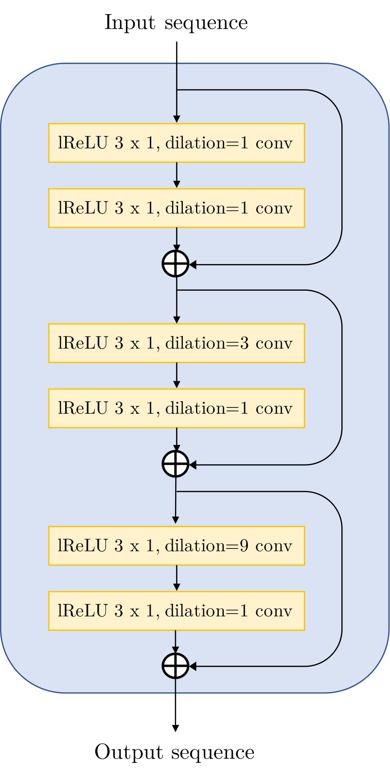
Figure 4: Residual Stack Architecture

图 4：残差堆叠结构

Appendix B Hyper-parameters and Training Details

附录 B 超参数与训练细节

We used a batch-size of 16 for all experiments. Adam, with learning rate 0.0001, $\beta_{1}=0.5$ and $\beta_{2}=0.9$ was used as the optimizer for both generator and discriminator. We used 10 as the coefficient for th feature-matching loss term. We used pytorch to implement our model, and its source code is accompanied with this submission. For VQGAN experiments, we used global latent vector of size 256, with KL term clamped below by 1.0 to avoid posterior collapse. We trained our models on Nvidia GTX1080Ti or GTX 2080Ti. In the supplementary material, we show reconstruction samples as a function of total number of epochs and wall-clock time. We find that our model starts producing intelligible samples very early in training.

所有实验批大小均为 16。生成器与判别器均用 Adam，学习率 0.0001，$\beta_{1}=0.5$，$\beta_{2}=0.9$。特征匹配损失项系数为 10。模型用 PyTorch 实现，源码随投稿附上。VQGAN 实验中全局潜向量维数为 256，KL 项下界钳制为 1.0 以避免后验坍缩。训练在 Nvidia GTX1080Ti 或 GTX 2080Ti 上进行。补充材料中给出重建样本随总 epoch 数与挂钟时间的变化；我们发现模型在训练很早期就开始产生可懂样本。

Appendix C Evaluation Method - MOS

附录 C 评测方法：MOS

We conducted Mean Opinion Score (MOS) tests to compare the performance of our model to competing architectures. We built the test by gathering samples generated by the different models as well as some original samples. All the generated samples were not seen during training. The MOS scores were computed on a population of 200 individuals: each of them was asked to blindly evaluate a subset of 15 samples taken randomly from this pool of samples by scoring samples from 1 to 5. The samples were presented and rated one at a time by the testers. The tests were crowdsourced using Amazon Mechanical Turk and we required the testers to wear headphones and be English speakers. After gathering all the evaluations, the MOS score $\mu_{i}$ of model $i$ is estimated by averaging the scores $m_{i,.}$ of the samples coming from the different models. In addition, we compute the 95% confidence intervals for the scores. $\hat{\sigma}_{i}$ being the standard deviation of the scores collected.

我们进行平均意见分（MOS）测试，以比较本模型与竞争结构的表现。测试集由不同模型生成的样本以及部分原始样本组成；所有生成样本均未在训练中见过。MOS 在 200 名受试者上计算：每人被要求盲评从该样本池中随机抽取的 15 个样本，按 1 到 5 打分；样本逐个呈现并打分。测试通过 Amazon Mechanical Turk 众包，要求受试者佩戴耳机且为英语使用者。汇总全部评测后，模型 $i$ 的 MOS 分 $\mu_{i}$ 由该模型样本得分 $m_{i,.}$ 平均得到；同时计算得分的 95% 置信区间。$\hat{\sigma}_{i}$ 为所收集得分的标准差。

$$\hat{\mu}_{i}=\frac{1}{N_{i}}\sum_{k=1}^{N_{i}}m_{i,k}$$

$$CI_{i}=\left[\hat{\mu}_{i}-1.96\frac{\hat{\sigma}_{i}}{\sqrt{N_{i}}},\hat{\mu}_{i}+1.96\frac{\hat{\sigma}_{i}}{\sqrt{N_{i}}}\right]$$