MegaSaM: Accurate, Fast, and Robust Structure and Motion from Casual Dynamic Videos

MegaSaM：从日常动态视频中准确、快速且鲁棒地估计结构与运动

Zhengqi Li    Richard Tucker    Forrester Cole    Qianqian Wang    Linyi Jin Affiliation:  Google DeepMind UC Berkeley University of Michigan    Vickie Ye    Angjoo Kanazawa    Aleksander Holynski    Noah Snavely

Abstract

摘要

We present a system that allows for accurate, fast, and robust estimation of camera parameters and depth maps from casual monocular videos of dynamic scenes. Most conventional structure from motion and monocular SLAM techniques assume input videos that feature predominantly static scenes with large amounts of parallax. Such methods tend to produce erroneous estimates in the absence of these conditions. Recent neural network-based approaches attempt to overcome these challenges; however, such methods are either computationally expensive or brittle when run on dynamic videos with uncontrolled camera motion or unknown field of view. We demonstrate the surprising effectiveness of a deep visual SLAM framework: with careful modifications to its training and inference schemes, this system can scale to real-world videos of complex dynamic scenes with unconstrained camera paths, including videos with little camera parallax. Extensive experiments on both synthetic and real videos demonstrate that our system is significantly more accurate and robust at camera pose and depth estimation when compared with prior and concurrent work, with faster or comparable running times. See interactive results on our project page: mega-sam.github.io.

我们提出一套系统，能从日常拍摄的动态场景单目视频中准确、快速且鲁棒地估计相机参数与深度图。多数传统运动恢复结构（SfM）与单目 SLAM 方法默认输入以静态场景为主、且视差充足；一旦不满足这些条件，估计就容易出错。近期基于神经网络的方法试图缓解这些问题，但要么计算昂贵，要么在相机运动不受控、视场未知的动态视频上很脆弱。我们展示了深度视觉 SLAM 框架的意外有效性：只要仔细修改其训练与推理方案，该系统就能扩展到相机轨迹不受限的复杂动态真实视频，包括几乎没有相机视差的视频。在合成与真实视频上的大量实验表明，与先前及同期工作相比，我们的系统在相机位姿与深度估计上显著更准、更稳，运行时间更快或相当。交互结果见项目页：mega-sam.github.io。

1 Introduction

1 引言

Extracting camera parameters and scene geometry from a set of images is a fundamental problem in computer vision, commonly referred to as structure from motion (SfM) or Simultaneous Localization and Mapping (SLAM). While decades of research have yielded mature algorithms for stationary scenes with large camera baselines, these methods often falter when applied to casual monocular videos captured in uncontrolled setting [26, 78]. Such videos, frequently captured by handheld cameras, typically exhibit limited camera motion parallax (e.g., nearly stationary or rotational cameras) and a broad range of focal lengths, and often include moving objects and scene dynamics. Recent efforts to address these challenges have focused on two primary strategies: optimizing camera and scene geometry by fine-tuning mono-depth networks or reconstructing radiance fields [35, 77, 78, 34]; or combining intermediate estimates derived from monocular video, such as depth, flows, long-term trajectory and motion segmentation, into a global optimization framework [26, 6, 76, 79, 34]. However, these approaches are computational expensive or brittle when applied to unconstrained videos that feature long time duration, unconstrained camera paths, or complex scene dynamics.

从一组图像中提取相机参数与场景几何，是计算机视觉的基本问题，通常称为运动恢复结构（SfM）或同步定位与建图（SLAM）。数十年研究已为「大基线静态场景」打磨出成熟算法，但把它们用到不受控环境下拍的日常单目视频时，往往力不从心[26, 78]。这类视频多由手持相机拍摄，相机运动视差有限（近乎静止或纯旋转），焦距范围很宽，还常含运动物体与场景动态。近期应对思路大致两类：通过微调单目深度网络或重建辐射场来联合优化相机与场景几何[35, 77, 78, 34]；或把单目视频中间估计（深度、光流、长程轨迹、运动分割等）塞进全局优化框架[26, 6, 76, 79, 34]。然而，一旦视频很长、相机路径不受限或场景动态复杂，这些方法要么很贵，要么很脆。

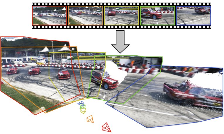
Figure 1: MegaSaM enables accurate, fast and robust estimation of cameras and scene structure from a casually captured monocular video of a dynamic scene. Top: input video frames (every tenth frame shown). Bottom: our estimated camera and 3D point clouds unprojected by predicted video depths without any postprocessing.

图 1：MegaSaM 能从日常拍摄的动态场景单目视频中，准确、快速且鲁棒地估计相机与场景结构。上：输入视频帧（每隔十帧显示）。下：我们估计的相机，以及由预测视频深度直接反投影得到的三维点云（未做后处理）。

In this work, we present MegaSaM, a full pipeline for accurate, fast and robust camera tracking and depth estimation from in-the-wild monocular videos of dynamic scenes. Our approach combines the strengths of several prior works, leading to results with previously unachievable quality, as shown in Fig. 1. In particular, we reexamine and extend prior deep visual SLAM framework for camera tracking. A defining feature of deep visual SLAM systems like DROID-SLAM [59] is that they adopt a differentiable bundle adjustment (BA) layer that iteratively updates scene geometry and camera pose variables, and intermediate predictions are learned from large amounts of data through camera and flow supervision. We find that such a learned layer is critical for achieving accurate and efficient camera pose estimation for the more challenging case of dynamic video. Building on this foundation, one of our key innovations for handling dynamic scene is to integrate monocular depth priors and motion probability maps into a differentiable SLAM paradigm.

本文提出 MegaSaM：面向野外动态场景单目视频的准确、快速且鲁棒相机跟踪与深度估计完整管线。方法综合多项先前工作的长处，达到此前难以企及的质量，见图 1。具体而言，我们重新审视并扩展了用于相机跟踪的深度视觉 SLAM 框架。像 DROID-SLAM[59] 这类系统的关键特征是采用可微光束法平差（BA）层，迭代更新场景几何与相机位姿，中间预测则通过相机与光流监督从大量数据中学得。我们发现，这种可学习层对动态视频这类更难设定下的准确高效位姿估计至关重要。在此基础上，我们的一项关键改动是把单目深度先验与运动概率图接入可微 SLAM 范式，以处理动态场景。

Further, we analyze the observability of structure and camera parameters in the video and introduce an uncertainty-aware global BA scheme, which improves system robustness when camera parameters are poorly constrained by the input video. We also demonstrate how consistent video depths can be accurately and efficiently obtained without the need for test-time network fine-tuning. Extensive evaluation on synthetic and real-world datasets demonstrates that our system significantly outperforms prior and concurrent baselines in both camera and depth estimation accuracy, while achieving competitive or superior runtime performance.

我们还分析视频中结构与相机参数的可观测性，引入感知不确定性的全局 BA 方案，从而在输入视频对相机参数约束很弱时提升系统鲁棒性。我们也展示了如何在无需测试时网络微调的情况下，准确且高效地得到一致的视频深度。在合成与真实数据集上的广泛评测表明，我们的系统在相机与深度估计精度上显著优于先前及同期基线，运行时间也具竞争力或更优。

2 Related Work

2 相关工作

Visual SLAM and SfM.

SLAM and SfM are used to estimate camera parameters and 3D scene structure from video sequences or unstructured image collections. Conventional approaches tackle this problem by first estimating 2D correspondence between images through feature matching [55, 1, 51, 44, 45, 5, 37, 8, 25, 56] or photometric alignment [38, 9, 10]. They then optimize 3D point locations and camera parameters by minimizing reprojection or photo-consistency errors through bundle adjustment (BA) [61].

视觉 SLAM 与 SfM。

SLAM 与 SfM 用于从视频序列或无结构图像集合估计相机参数与三维场景结构。传统方法先通过特征匹配[55, 1, 51, 44, 45, 5, 37, 8, 25, 56]或光度对齐[38, 9, 10]估计图像间二维对应，再经光束法平差（BA）[61]最小化重投影或光度一致性误差，优化三维点位置与相机参数。

Recently, deep visual SLAM and SfM systems have emerged that adopt deep neural networks to estimate pairwise or long-term correspondences [2, 57, 65, 73, 60, 59, 63, 54, 7, 18, 21, 19], to reconstruct radiance fields [33, 11, 41] or global 3D point clouds [28, 66]. While these methods demonstrate accurate camera tracking and reconstruction, they typically assume predominantly static scenes and sufficient camera baselines between frames. Therefore, their performance can degrade significantly or fail entirely in the presence of scene dynamics or limited camera parallax.

近年出现了深度视觉 SLAM 与 SfM 系统：用深度网络估计成对或长程对应[2, 57, 65, 73, 60, 59, 63, 54, 7, 18, 21, 19]，重建辐射场[33, 11, 41]或全局三维点云[28, 66]。这些方法在相机跟踪与重建上往往很准，但通常假设场景以静态为主、帧间基线充足；一旦出现场景动态或视差不足，性能会明显下降甚至完全失败。

Several recent works share similar goals with ours in addressing these limitations. Robust-CVD [26] and CasualSAM [78] jointly estimate camera parameters and dense depth maps from dynamic videos by optimizing a spatially varying spline or fine-tuning monocular depth networks. Particle-SfM [79] and LEAP-VO [6] first infer moving object masks based on long-range trajectories, then use this information to downweight the contribution of the features during bundle adjustment. Concurrent work, MonST3R [76], adopts a 3D point cloud representation from DuST3R [66] and localizes cameras via an additional alignment optimization. Our approach shares similar ideas, but we show that performance can be significantly improved by coupling the differentiable SLAM system with the intermediate predictions of underlying dynamic scenes.

若干近期工作与我们目标相近，也试图突破这些限制。Robust-CVD[26] 与 CasualSAM[78] 通过对空间变化样条做优化或微调单目深度网络，从动态视频联合估计相机参数与稠密深度。Particle-SfM[79] 与 LEAP-VO[6] 先根据长程轨迹推断运动物体掩码，再在 BA 中下调对应特征的贡献。同期工作 MonST3R[76] 采用 DuST3R[66] 的三维点云表示，再经额外对齐优化定位相机。我们的思路相近，但表明：把可微 SLAM 系统与底层动态场景的中间预测耦合起来，性能可以显著提升。

Monocular depth.

Recent work on monocular depth prediction has shown strong generalization on in-the-wild single images by training deep neural networks on large amounts of synthetic and real-world data [29, 30, 47, 74, 46, 49, 71, 72, 75, 43, 22, 13]. However, these single-image models tend to produce temporally inconsistent depth from videos. To overcome this issue, prior techniques propose to fine-tune mono-depth models by performing test-time optimization [35, 77] or to use transformer or diffusion models to directly predict video depths [69, 53, 20]. Our approach follows the spirit of the first paradigm, but we show that we can achieve better video depth quality without resorting to expensive network fine-tuning for every video.

单目深度。

近期单目深度预测工作通过在大量合成与真实数据上训练深度网络，在野外单图上展现出强泛化[29, 30, 47, 74, 46, 49, 71, 72, 75, 43, 22, 13]。但这些单图模型对视频往往会给出时间上不一致的深度。为缓解该问题，已有技术对单目深度模型做测试时优化微调[35, 77]，或用 Transformer、扩散模型直接预测视频深度[69, 53, 20]。我们的方法沿袭第一类范式的精神，但表明不必对每个视频做昂贵的网络微调，也能得到更好的视频深度质量。

Dynamic scene reconstruction.

Several recent works have adopted time-varying radiance field representations to perform dynamic scene reconstruction and novel view synthesis from in-the-wild videos [39, 40, 31, 32, 12, 67, 27, 64, 34, 70]. Our work is orthogonal to most of these techniques since most radiance field reconstruction methods require camera parameters or video depth maps as inputs, and our outputs can be used as inputs to these systems.

动态场景重建。

若干近期工作采用时变辐射场表示，从野外视频做动态场景重建与新视角合成[39, 40, 31, 32, 12, 67, 27, 64, 34, 70]。我们的工作与其中多数正交：多数辐射场重建方法需要相机参数或视频深度作为输入，而我们的输出可直接作为这些系统的输入。

3 MegaSaM

Given an unconstrained, continuous video sequence $\mathcal{V}=\{I_{i}\in\mathcal{R}^{H\times W}\}^{N}_{i=1}$ our goal is to estimate camera poses $\hat{\mathbf{G}}_{i}\in SE(3)$, focal length $\hat{f}$ (if unknown), and dense video depth maps $\mathcal{D}=\{\hat{D}_{i}\}^{N}_{i=1}$. Our approach does not pose any constraints on the camera and object motions present in the input video. Our camera tracking and video depth estimation modules build upon prior deep visual SLAM (in particular, DROID-SLAM [59]) and casual structure and motion [78] frameworks, respectively.

给定不受限的连续视频序列 $\mathcal{V}=\{I_{i}\in\mathcal{R}^{H\times W}\}^{N}_{i=1}$，目标是估计相机位姿 $\hat{\mathbf{G}}_{i}\in SE(3)$、焦距 $\hat{f}$（若未知），以及稠密视频深度图 $\mathcal{D}=\{\hat{D}_{i}\}^{N}_{i=1}$。我们对输入视频中的相机与物体运动不加任何约束。相机跟踪与视频深度估计模块分别建立在先前深度视觉 SLAM（尤其是 DROID-SLAM[59]）与日常结构运动[78]框架之上。

In the following section, we first summarize the key components of a deep visual SLAM framework designed for tracking videos of static scenes with sufficient camera motion parallax (Sec. 3.1). We then introduce key modifications to this framework, at both the training and inference stages, that enable fast, robust and accurate camera tracking for unconstrained dynamic videos (Sec. 3.2). Finally, we demonstrate how to efficiently estimate consistent video depths given the estimated camera parameters (Sec. 3.3).

下文首先概括面向「静态场景、相机视差充足」视频的深度视觉 SLAM 框架关键组件（第 3.1 节）；再介绍对该框架在训练与推理两端的关键修改，使其能对不受限动态视频做快速、鲁棒且准确的相机跟踪（第 3.2 节）；最后说明如何在已估计相机参数下高效估计一致视频深度（第 3.3 节）。

3.1 Deep visual SLAM formulation

3.1 深度视觉 SLAM 表述

Deep visual SLAM systems like DROID-SLAM [59] are characterized by a differentiable, learned bundle adjustment (BA) layer that iteratively updates structure and motion parameters. In particular, they keep track of two state variables while processing a video: a per-frame low-resolution disparity map $\hat{\mathbf{d}}_{i}\in\mathcal{R}^{\frac{H}{8}\times\frac{W}{8}}$, and camera poses $\hat{\mathbf{G}}_{i}\in SE(3)$. These variables are updated iteratively during both training and inference stages through the differentiable BA layer, which operates over a set of image pairs from a frame-graph $(I_{i},I_{j})\in\mathcal{P}$, built dynamically to connect frames with overlapping field of view.

像 DROID-SLAM[59] 这类深度视觉 SLAM 系统的特征是可微、可学习的光束法平差（BA）层，迭代更新结构与运动参数。处理视频时，它们维护两类状态变量：每帧低分辨率视差图 $\hat{\mathbf{d}}_{i}\in\mathcal{R}^{\frac{H}{8}\times\frac{W}{8}}$，以及相机位姿 $\hat{\mathbf{G}}_{i}\in SE(3)$。训练与推理阶段都通过可微 BA 层迭代更新这些变量；BA 作用在帧图 $(I_{i},I_{j})\in\mathcal{P}$ 的一组图像对上，该图动态构建以连接视野重叠的帧。

Given two video frames $I_{i}$ and $I_{j}$ from the frame graph as input, DROID-SLAM learns to predict a 2D correspondence field ${\hat{\mathbf{u}}}_{ij}\in\mathcal{R}^{\frac{H}{8}\times\frac{W}{8}\times 2}$ and a confidence $\hat{\mathbf{w}}_{ij}\in\mathcal{R}^{\frac{H}{8}\times\frac{W}{8}}$ through convolutional gated recurrent units in an iterative manner: $({\hat{\mathbf{u}}}_{ij}^{k+1},\hat{\mathbf{w}}_{ij}^{k+1})=F(I_{i},I_{j},{\hat{\mathbf{u}}}_{ij}^{k},\hat{\mathbf{w}}_{ij}^{k})$, where $k$ denotes the $k^{th}$ iteration. In addition, the rigid-motion correspondence field can also be derived from the camera ego-motion and the disparity through a multi-view constraint:

给定帧图中的两帧 $I_{i}$ 与 $I_{j}$，DROID-SLAM 用卷积门控循环单元迭代学习预测二维对应场 ${\hat{\mathbf{u}}}_{ij}\in\mathcal{R}^{\frac{H}{8}\times\frac{W}{8}\times 2}$ 与置信度 $\hat{\mathbf{w}}_{ij}\in\mathcal{R}^{\frac{H}{8}\times\frac{W}{8}}$：$({\hat{\mathbf{u}}}_{ij}^{k+1},\hat{\mathbf{w}}_{ij}^{k+1})=F(I_{i},I_{j},{\hat{\mathbf{u}}}_{ij}^{k},\hat{\mathbf{w}}_{ij}^{k})$，其中 $k$ 表示第 $k$ 次迭代。此外，刚体运动对应场也可由相机自运动与视差经多视图约束导出：

$${{\mathbf{u}}_{ij}}=\pi\left(\hat{\mathbf{G}}_{ij}\circ\pi^{-1}(\mathbf{p}_{i},\hat{\mathbf{d}}_{i},K^{-1}),K\right), \tag{1}$$

where $\mathbf{p}_{i}$ denotes a grid of pixel coordinates, $\pi$ denotes the perspective projection operator, $\hat{\mathbf{G}}_{ij}=\hat{\mathbf{G}}_{j}\circ\hat{\mathbf{G}}^{-1}_{i}$ is the relative camera pose between $I_{i}$ and $I_{j}$, and $K\in\mathcal{R}^{3\times 3}$ denotes the camera intrinsic matrix.

其中 $\mathbf{p}_{i}$ 表示像素坐标网格，$\pi$ 为透视投影算子，$\hat{\mathbf{G}}_{ij}=\hat{\mathbf{G}}_{j}\circ\hat{\mathbf{G}}^{-1}_{i}$ 是 $I_{i}$ 与 $I_{j}$ 之间的相对相机位姿，$K\in\mathcal{R}^{3\times 3}$ 为相机内参矩阵。

Differentiable bundle adjustment. DROID-SLAM assumes known focal length, but focal length is typically not known a priori for in-the-wild videos. Therefore, we optimize camera poses, focal length and disparity by iteratively minimizing a weighted reprojection cost between the current flows predicted by the network and the rigid-motion ones derived from camera parameters and disparity [16]:

可微光束法平差。 DROID-SLAM 假定焦距已知，但野外视频通常事先不知道焦距。因此，我们通过迭代最小化网络当前预测光流与由相机参数、视差导出的刚体运动光流之间的加权重投影代价，来联合优化相机位姿、焦距与视差[16]：

$$\mathcal{C}(\hat{\mathbf{G}},\hat{\mathbf{d}},\hat{f})=\sum_{(i,j)\in\mathcal{P}}||{\hat{\mathbf{u}}}_{ij}-{\mathbf{u}}_{ij}||_{\Sigma_{ij}}^{2} \tag{2}$$

where weights $\Sigma_{ij}=\text{diag}(\hat{\mathbf{w}}_{ij})^{-1}$. To enable differentiable end-to-end training, we perform optimization of Eq. 2 with the Levenberg–Marquardt algorithm:

其中权重 $\Sigma_{ij}=\text{diag}(\hat{\mathbf{w}}_{ij})^{-1}$。为支持端到端可微训练，我们用 Levenberg–Marquardt 算法优化式 2：

$$\left(\mathbf{J}^{T}\mathbf{W}\mathbf{J}+\lambda\text{diag}({\mathbf{J}^{T}\mathbf{W}\mathbf{J}})\right)\Delta\boldsymbol{\xi}=\mathbf{J}^{T}\mathbf{W}\mathbf{r} \tag{3}$$

where $\Delta\boldsymbol{\xi}=(\Delta\mathbf{G},\Delta\mathbf{d},\Delta f)^{T}$ is the parameter updates of the state variables, $\mathbf{J}$ is the Jacobian of reprojection residuals w.r.t. the parameters, and $\mathbf{W}$ is a diagonal matrix containing $\hat{\mathbf{w}}_{ij}$ from each frame pair. $\lambda$ is a damping factor predicted by the network during each BA iteration. We can separate camera parameters (including poses and focal length) and disparity variables by dividing the approximated Hessian on the LHS of Eq. 3 into following block matrix form:

其中 $\Delta\boldsymbol{\xi}=(\Delta\mathbf{G},\Delta\mathbf{d},\Delta f)^{T}$ 是状态变量的参数更新，$\mathbf{J}$ 是重投影残差对参数的雅可比，$\mathbf{W}$ 是包含各帧对 $\hat{\mathbf{w}}_{ij}$ 的对角矩阵。$\lambda$ 是每次 BA 迭代中由网络预测的阻尼因子。把式 3 左侧的近似 Hessian 写成如下分块形式，即可分开相机参数（含位姿与焦距）与视差变量：

$$\displaystyle\begin{bmatrix}\mathbf{H}{\mathbf{G},f}&\mathbf{E}{\mathbf{G},f}\
\mathbf{E}{\mathbf{G},f}^{T}&\mathbf{H}{\mathbf{d}}\end{bmatrix}\begin{bmatrix}\Delta\boldsymbol{\xi}{\mathbf{G},f}\
\Delta\mathbf{d}\
\end{bmatrix}=\begin{bmatrix}\tilde{r}{\mathbf{G},f}\
\tilde{r}_{\mathbf{d}}\
\end{bmatrix} \tag{4}$$

Since only a single disparity variable is included in each pairwise reprojection term from Eq. 2, $\mathbf{H}_{\mathbf{d}}$ in Eq. 4 is a diagonal matrix, and hence we can efficiently compute parameter updates using the Schur complement trick [61], which leads to fully differentiable BA update:

由于式 2 的每个成对重投影项只包含一个视差变量，式 4 中的 $\mathbf{H}_{\mathbf{d}}$ 是对角阵，因而可用 Schur 补技巧[61]高效计算参数更新，从而得到完全可微的 BA 更新：

$$\displaystyle\Delta\boldsymbol{\xi}_{\mathbf{G},f} \\ \displaystyle=\left[\mathbf{H}_{\mathbf{G},f}-\mathbf{E}_{\mathbf{G},f}\mathbf{H}_{\mathbf{d}}^{-1}{\mathbf{E}_{\mathbf{G},f}}^{T}\right]^{-1}(\tilde{r}_{\mathbf{G},f}-\mathbf{E}_{\mathbf{G},f}\mathbf{H}_{\mathbf{d}}^{-1}\tilde{r}_{\mathbf{d}}) \\ \displaystyle\Delta\mathbf{z} \\ \displaystyle=\mathbf{H}_{\mathbf{d}}^{-1}(\tilde{r}_{\mathbf{d}}-\mathbf{E}_{\mathbf{G},f}^{T}\Delta\boldsymbol{\xi}_{\mathbf{G},f}) \tag{5}$$

Training. The flow and uncertainty predictions are trained end-to-end from a collection of synthetic video sequences of static scenes:

训练。 光流与不确定性预测在静态场景合成视频集合上端到端训练：

$$\displaystyle\mathcal{L}_{\text{static}}=\mathcal{L}_{\text{cam}}+w_{\text{flow}}\mathcal{L}_{\text{flow}} \tag{7}$$

where $\mathcal{L}_{\text{cam}}$ and $\mathcal{L}_{\text{flow}}$ are losses comparing estimated camera parameters and ego-motion induced flows from the BA layer with corresponding ground truths.

其中 $\mathcal{L}_{\text{cam}}$ 与 $\mathcal{L}_{\text{flow}}$ 将 BA 层估计的相机参数及自运动诱导光流与对应真值比较。

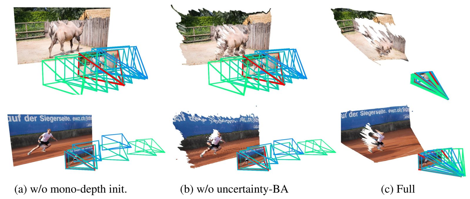
Figure 2: Ablation on our design choices. From left to right, we visualize cameras and reconstruction from our system (a) without mono-depth initialization, (b) without uncertainty-aware BA, (c) with full configuration. For these difficult near-rotational sequences, our full method produces much better camera and scene geometry.

图 2：设计选择消融。从左到右可视化：(a) 无单目深度初始化；(b) 无感知不确定性 BA；(c) 完整配置下的相机与重建。对这些困难的近纯旋转序列，完整方法给出明显更好的相机与场景几何。

3.2 Scaling to in-the-wild dynamic videos

3.2 扩展到野外动态视频

Deep Visual SLAM works reasonably well for videos that feature static scenes and have sufficient camera translation, but its performance degrades when operating on videos of dynamic content, or videos with limited parallax, as shown in the first column of Fig. 2. To overcome these issues, we propose key modifications to the original training and inference pipeline. First, our model predicts object movement maps that are learned together with flow and uncertainty in order to downweight dynamic elements within the differentiable BA layer. Second, we propose to integrate priors from mono-depth estimates into the both training and inference pipeline, and perform uncertainty-aware global BA, both of which aid disambiguation of object and camera motion in challenging casual dynamic videos. Our system is trained on synthetic data alone, but we demonstrate its strong generalization to real-world videos.

深度视觉 SLAM 对静态场景、相机平移充足的视频通常表现不错，但一遇到动态内容或视差有限的视频，性能就会下降，见图 2 第一列。为克服这些问题，我们对原训练与推理管线做了关键修改。第一，模型预测物体运动图，与光流、不确定性一并学习，以便在可微 BA 层中下调动态元素的权重。第二，把单目深度估计先验接入训练与推理，并做感知不确定性的全局 BA，二者都有助于在困难的日常动态视频中消歧物体运动与相机运动。系统仅在合成数据上训练，但对真实视频展现出强泛化。

3.2.1 Training

Learning motion probability. Recall from Sec. 3.1 that for every selected image pair $(I_{i},I_{j})\in\mathcal{P}$, our model predicts a 2D flow ${\hat{\mathbf{u}}}_{ij}$ and associated confidence $\hat{\mathbf{w}}_{ij}$ at each BA iteration, and that these predictions are supervised from synthetic sequences of static scenes. To extend the model to handle dynamic scenes, we can directly train the model predictions on videos of dynamic scenes with corresponding ground truth supervision, hoping that the pairwise uncertainty will subsume the object motion information automatically during training. However, we find that this simple training strategy tends to produce suboptimal results due to unstable training behaviour from differentiable BA layers.

3.2.1 训练

学习运动概率。 回顾第 3.1 节：对每个选定图像对 $(I_{i},I_{j})\in\mathcal{P}$，模型在每次 BA 迭代预测二维光流 ${\hat{\mathbf{u}}}_{ij}$ 与置信度 $\hat{\mathbf{w}}_{ij}$，这些预测由静态场景合成序列监督。为扩展到动态场景，可以直接在带真值监督的动态视频上训练模型预测，指望成对不确定性在训练中自动吸收物体运动信息。但我们发现，这种简单策略常因可微 BA 层训练不稳定而效果不佳。

Instead, we propose to use an additional network $F_{m}$ to iteratively predict an object movement probability map $\mathbf{m}_{i}\in\mathcal{R}^{\frac{H}{8}\times\frac{W}{8}}=F_{m}\left(\{I_{i}\}\cup\mathcal{N}(i)\right)$ conditioned on $I_{i}$ and a set of its neighboring keyframes $\mathcal{N}(i)=\{I_{j}|(i,j)\in\mathcal{P}\}$. This movement map is specifically supervised to predict pixels that correspond to dynamic content based on multi-frame information. During each BA iteration, we combine pairwise flow confidence $\hat{\mathbf{w}}_{ij}$ with object movement map $\mathbf{m}_{i}$ to form the final weights in Eq. 2: ${\tilde{\mathbf{w}}}_{ij}=\hat{\mathbf{w}}_{ij}\mathbf{m}_{i}$.

我们改为用额外网络 $F_{m}$ 迭代预测物体运动概率图 $\mathbf{m}_{i}\in\mathcal{R}^{\frac{H}{8}\times\frac{W}{8}}=F_{m}\left(\{I_{i}\}\cup\mathcal{N}(i)\right)$，条件是 $I_{i}$ 及其邻域关键帧集合 $\mathcal{N}(i)=\{I_{j}|(i,j)\in\mathcal{P}\}$。该运动图专门监督去预测对应动态内容的像素，依据多帧信息。每次 BA 迭代中，把成对光流置信度 $\hat{\mathbf{w}}_{ij}$ 与物体运动图 $\mathbf{m}_{i}$ 组合成式 2 的最终权重：${\tilde{\mathbf{w}}}_{ij}=\hat{\mathbf{w}}_{ij}\mathbf{m}_{i}$。

Moreover, we design a two-stage training scheme that trains the models on a mixture of static and dynamic videos to effectively learn 2D flows along with the movement probability maps. In the first ego-motion pretraining stage, we train the original deep SLAM model $F$ by supervising the predicted flows and confidence maps (using the losses in Eq. 7) with synthetic data of static scenes, i.e., without any dynamic video data. This stage helps model effectively learn pairwise flows and corresponding confidence induced only by ego-motion. In the second dynamic fine-tuning stage, we freeze the parameters of $F$ and finetune $F_{m}$ on synthetic dynamic videos, conditioning $F_{m}$ on the features from our pretrained $F$ during each iteration to predict movement probability map $\mathbf{m}_{i}$, supervising through both camera and cross-entropy losses:

此外，我们设计两阶段训练方案：在静态与动态视频的混合上训练模型，以有效学习二维光流与运动概率图。第一阶段自运动预训练中，用静态场景合成数据（即不含任何动态视频）按式 7 的损失监督预测光流与置信图，训练原始深度 SLAM 模型 $F$。该阶段帮助模型有效学习仅由自运动诱导的成对光流及对应置信度。第二阶段动态微调中，冻结 $F$ 的参数，在合成动态视频上微调 $F_{m}$，每次迭代让 $F_{m}$ 条件于预训练 $F$ 的特征以预测运动概率图 $\mathbf{m}_{i}$，并用相机损失与交叉熵损失共同监督：

$$\mathcal{L}_{\text{dynamic}}=\mathcal{L}_{\text{cam}}+w_{\text{motion}}\mathcal{L}_{\text{CE}} \tag{8}$$

This stage decorrelates learning scene dynamics from learning 2D correspondences, and thus leads to more stable and effective training behavior for the differentiable BA framework. We found this training scheme to be critical for producing accurate camera estimation results for dynamic videos, as shown in our ablation study. We visualize learned motion probability maps $\mathbf{m}_{i}$ in Fig. 3.

该阶段把学习场景动态与学习二维对应解耦，从而使可微 BA 框架的训练更稳、更有效。消融表明，这一训练方案对动态视频上的准确相机估计至关重要。学到的运动概率图 $\mathbf{m}_{i}$ 可视化见图 3。

Disparity and camera initialization. DROID-SLAM initializes disparity $\hat{\mathbf{d}}$ by simply setting it to a constant value of $1$. However, we find that this initialization fails to perform accurate camera tracking on videos with limited camera baselines and complex scene dynamics. Inspired by recent work [31, 64, 32, 34], during both the training and inference stages, we perform data-driven initialization by integrating a mono-depth prior. During training, we initialize $\hat{\mathbf{d}}$ with disparity from DepthAnything [71] with the estimated global scale and shift borrowed from the ground truth depth of each training sequence. For each training sequence, we initialize first two camera poses to the ground-truth to remove the gauge ambiguity, and initialize the camera focal length by randomly perturbing the ground truth value by $25\%$.

视差与相机初始化。 DROID-SLAM 把视差 $\hat{\mathbf{d}}$ 简单初始化为常数 1。但我们发现，在相机基线有限、场景动态复杂的视频上，这种初始化无法做准相机跟踪。受近期工作启发[31, 64, 32, 34]，训练与推理阶段都接入单目深度先验做数据驱动初始化。训练时，用 DepthAnything[71] 的视差初始化 $\hat{\mathbf{d}}$，全局尺度与平移借自每条训练序列的真值深度。对每条训练序列，把前两帧相机位姿初始化为真值以消除规范自由度，焦距则在真值基础上随机扰动 25% 作为初始化。

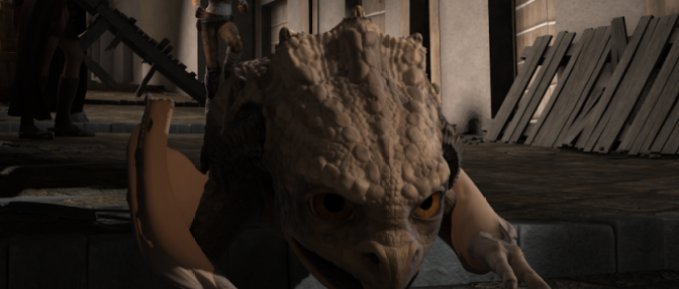
I Image	I Motion probability

Figure 3: Learned movement map. Left: input video frame, right: corresponding learned motion probability map.

I 图像	I 运动概率

图 3：学到的运动图。左：输入视频帧；右：对应的学到的运动概率图。

3.2.2 Inference

Our inference pipeline consists of two components: (i) a frontend module registers cameras for keyframes by performing frame selection followed by a sliding window BA. (ii) a backend module refines the estimates by performing global BA over all video frames. In this subsection, we describe the modifications we made at inference.

3.2.2 推理

推理管线含两部分：(i) 前端模块通过选帧与滑动窗口 BA 为关键帧登记相机；(ii) 后端模块对全部视频帧做全局 BA 以精炼估计。本节描述推理阶段的修改。

Initialization and frontend tracking. Similar to training, we incorporate both mono-depth and focal length predictions into the inference pipeline. In particular, we initialize per-frame disparity maps $\hat{\mathbf{d}}_{i}$ with metric aligned monocular disparity $D^{\text{align}}_{i}=\hat{\alpha}D^{\text{rel}}_{i}+\hat{\beta}$, where $D^{\text{rel}}_{i}$ is per-frame affine-invariant disparity from [71], and per-video global scale and shift parameters $(\hat{\alpha},\hat{\beta})$ are estimated through median aligning $D^{\text{rel}}_{i}$ with an additional metric depth estimates $D^{\text{abs}}_{i}$ from UniDepth [43]: $\hat{\alpha}_{i}=\frac{D^{\text{abs}}_{i}-\text{median}_{i}(D^{\text{abs}}_{i})}{D^{\text{rel}}_{i}-\text{median}(D^{\text{rel}}_{i})}$; $\hat{\beta}=\text{median}\left(D^{\text{abs}}_{i}-\hat{\alpha}D^{\text{rel}}_{i}\right)$.[^1] The UniDepth model also predicts the focal length of each frame; we use the median estimate across the video frames to obtain an initial focal length estimate $\hat{f}$, which is fixed within the frontend stage.

初始化与前端跟踪。 与训练类似，推理管线也接入单目深度与焦距预测。具体地，用度量对齐的单目视差 $D^{\text{align}}_{i}=\hat{\alpha}D^{\text{rel}}_{i}+\hat{\beta}$ 初始化每帧视差图 $\hat{\mathbf{d}}_{i}$，其中 $D^{\text{rel}}_{i}$ 来自[71]的每帧仿射不变视差，每视频全局尺度与平移 $(\hat{\alpha},\hat{\beta})$ 通过把 $D^{\text{rel}}_{i}$ 与 UniDepth[43] 的额外度量深度 $D^{\text{abs}}_{i}$ 做中位数对齐估计：$\hat{\alpha}_{i}=\frac{D^{\text{abs}}_{i}-\text{median}_{i}(D^{\text{abs}}_{i})}{D^{\text{rel}}_{i}-\text{median}(D^{\text{rel}}_{i})}$；$\hat{\beta}=\text{median}\left(D^{\text{abs}}_{i}-\hat{\alpha}D^{\text{rel}}_{i}\right)$。[1] UniDepth 也预测每帧焦距；我们取全视频帧的中位数作为初始焦距估计 $\hat{f}$，并在前端阶段固定。

To initialize the SLAM system, we accumulate keyframes with sufficient pairwise motion until we have a set of $N_{\text{init}}=8$ active images. We initialize camera poses for these keyframes by performing camera motion–only bundle adjustment while fixing disparity variables $\hat{\mathbf{d}}_{i}$ to aligned monocular disparity $D^{\text{align}}_{i}$. After initialization, we incrementally add new keyframes, remove old keyframes, and perform local BA in a sliding window manner, where each keyframe disparity is also initialized to aligned mono-disparity. In this stage, the BA cost function consists of a reprojection error and a mono-depth regularization term:

为初始化 SLAM 系统，我们累积具有足够成对运动的关键帧，直到活跃图像数达到 $N_{\text{init}}=8$。对这些关键帧，在把视差变量 $\hat{\mathbf{d}}_{i}$ 固定为对齐单目视差 $D^{\text{align}}_{i}$ 的同时，仅做相机运动 BA 以初始化位姿。初始化后，以滑动窗口方式增量加入新关键帧、移除旧关键帧并做局部 BA，每个关键帧视差同样初始化为对齐单目视差。此阶段 BA 代价由重投影误差与单目深度正则项组成：

$$\mathcal{C}=\sum_{(i,j)\in\mathcal{P}}||{\hat{\mathbf{u}}}_{ij}-{\mathbf{u}}_{ij}||_{\Sigma_{ij}}^{2}+w_{d}\sum_{i}||\hat{\mathbf{d}}_{i}-D^{\text{align}}_{i}||^{2}. \tag{9}$$

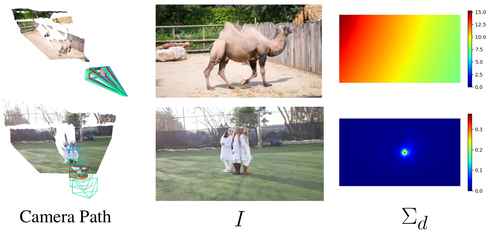
Figure 4: Visualization of epistemic uncertainty. From left to right, we visualize camera paths, reference image and corresponding epistemic uncertainty of disparity. The geometry is not observable from the top example with little camera parallax, as indicated by the larger uncertainty. The peak on the bottom uncertainty map corresponds to the epipole for forward moving motion.

图 4：认知不确定性可视化。从左到右：相机路径、参考图像及对应视差的认知不确定性。上例相机视差很小，几何不可观测，表现为更大的不确定性。下例不确定性图上的峰值对应前向运动的对极点。

Uncertainty-aware global BA. The backend module first performs global BA over all keyframes. The module then performs a pose-graph optimization to register the poses of non-keyframes. Finally, the backend module refines the entire camera trajectory via a global BA over all video frames.

感知不确定性的全局 BA。 后端模块先对全部关键帧做全局 BA，再经位姿图优化登记非关键帧位姿，最后对全体视频帧再做一次全局 BA，精炼整条相机轨迹。

This design raises a question: should we (or when should we) add mono-depth regularization from Eq. 9 into the global bundle adjustment? One on hand, if there is sufficient camera baseline in the input video, we observe that mono-depth regularization isn’t needed, since the problem is already well-constrained and in fact the error from mono-depth can diminish camera tracking accuracy. On the other hand, if a video is captured from a rotational camera with little camera baseline, then performing a reprojection-only BA without additional constraints can lead to degenerate solutions, as shown in the second column of Fig. 2.

这引出一个问题：是否（以及何时）应把式 9 的单目深度正则加入全局光束法平差？一方面，若输入视频相机基线充足，我们观察到并不需要单目深度正则——问题本身已良好约束，单目深度误差反而会削弱相机跟踪精度。另一方面，若视频来自基线极小的旋转相机，仅做重投影 BA、不加额外约束，可能得到退化解，见图 2 第二列。

To see why, we explore the approximate Hessian matrix from the linear system in Eq. 4. As shown by Goli et al. [14], given the posterior, $p(\theta|\mathcal{I})$, we can use Laplace approximations to estimate the covariance $\Sigma$ of the variables through the inverse Hessian: $\Sigma_{\theta}=-\mathbf{H}(\theta^{*})^{-1}$, where $\theta^{*}$ is the MAP estimate of the parameters and $\Sigma_{\theta}$ denotes the epistemic uncertainty of estimated variables [23]. Since inverting the full Hessian is computationally expensive when the number of input frames is large, we follow Ritter et al. [48] and approximate $\Sigma_{\theta}$ through the diagonal of the Hessian:

为理解原因，我们考察式 4 线性系统中的近似 Hessian。如 Goli 等[14]所示，给定后验 $p(\theta|\mathcal{I})$，可用 Laplace 近似通过逆 Hessian 估计变量协方差 $\Sigma$：$\Sigma_{\theta}=-\mathbf{H}(\theta^{*})^{-1}$，其中 $\theta^{*}$ 是参数的 MAP 估计，$\Sigma_{\theta}$ 表示估计变量的认知不确定性[23]。完整 Hessian 在输入帧很多时求逆很贵，我们按 Ritter 等[48]用 Hessian 对角近似 $\Sigma_{\theta}$：

$$\Sigma_{\theta}\approx\text{diag}\left(-\mathbf{H}(\theta^{*})\right)^{-1} \tag{10}$$

Intuitively, when we consider the reprojection error in Eq. 2, the Jacobian of estimated variables $\mathbf{J}_{\theta}$ indicates how much the reprojection error would change if we perturb the variables. Therefore, the uncertainty $\Sigma_{\theta}$ is large when perturbing the parameters has little impact on the reprojection error. Specifically, let us consider the disparity variables, and consider an extreme case where the input video is captured by a static camera. In this case, the pairwise reprojection error would be unchanged as a function of disparity, implying a large uncertainty in the estimated disparity; that is, the disparity is unobservable from the video alone. We visualize the spatial uncertainty of the estimated normalized disparity $\Sigma_{d}$ in Fig 4: the first row shows a video featuring rotational dominant motion, whereas the second row shows videos captured by a forward-moving camera. From the color bars in the third column, we see the range of disparity uncertainty $\Sigma_{d}$ is much higher in the first example.

直观上，考虑式 2 的重投影误差时，估计变量的雅可比 $\mathbf{J}_{\theta}$ 表明扰动变量会让重投影误差变化多少。因此，当扰动参数几乎不影响重投影误差时，不确定性 $\Sigma_{\theta}$ 很大。具体看视差变量，考虑输入由静止相机拍摄的极端情形：成对重投影误差作为视差的函数不变，意味着估计视差不确定性很大，即仅凭视频无法观测视差。图 4 可视化估计归一化视差的空间不确定性 $\Sigma_{d}$：第一行是旋转主导运动的视频，第二行是前向运动相机拍摄的视频。从第三列色条可见，第一例中视差不确定性 $\Sigma_{d}$ 的范围高得多。

Such uncertainty quantification gives us a measure for observability of camera and disparity parameters, allowing us to decide where we should add mono-depth regularization (and additionally when we should turn off camera focal length optimization). In practice, we find that simply checking the median uncertainty of normalized disparity and uncertainty of normalized focal length works well for all the videos we tested. In particular, after completing frontend tracking, we retrieve the diagonal entry of disparity Hessian formed from all the keyframes and compute its median $\text{med}\left(\text{diag}(\mathbf{H}_{\mathbf{d}})\right)$, as well as the Hessian entry of the shared focal length ${H}_{f}$. We then set the mono-depth regularization weight based on the median disparity Hessian $w_{d}=\gamma_{d}\exp\left(-\beta_{d}\text{med}\left(\text{diag}(\mathbf{H}_{\mathbf{d}})\right)\right)$. In other words, we enable mono-depth regularization if the camera poses are unobservable from the input video alone due to limited camera motion parallax. In addition, we disable focal length optimization if ${H}_{f}<\tau_{f}$, since this condition indicates that focal length is likely unobservable from the input.

这种不确定性量化给出相机与视差参数可观测性的度量，从而决定何处应加单目深度正则（以及何时应关闭焦距优化）。实践中，我们发现简单检查归一化视差的中位不确定性与归一化焦距的不确定性，对测试过的全部视频都够用。具体地，前端跟踪完成后，取出由全部关键帧构成的视差 Hessian 对角元并计算其中位数 $\text{med}\left(\text{diag}(\mathbf{H}_{\mathbf{d}})\right)$，以及共享焦距的 Hessian 元 ${H}_{f}$。再按中位视差 Hessian 设定单目深度正则权重 $w_{d}=\gamma_{d}\exp\left(-\beta_{d}\text{med}\left(\text{diag}(\mathbf{H}_{\mathbf{d}})\right)\right)$。换言之，若因相机运动视差有限、仅凭输入视频无法观测相机位姿，就启用单目深度正则。此外，若 ${H}_{f}<\tau_{f}$，则关闭焦距优化，因为该条件表明焦距很可能从输入中不可观测。

3.3 Consistent depth optimization

3.3 一致深度优化

Optionally, one can obtain more accurate and consistent video depth at higher resolution than the estimated low-res disparity variables given the estimated camera parameters.

可选地，在已估计相机参数后，还能以高于低分辨率视差变量的分辨率，得到更准确、更一致的视频深度。

In particular, we follow CasualSAM [78] and perform an additional first-order optimization on video depths along with per-frame aleatoric uncertainty maps. Our objective consist of three cost functions:

具体地，我们遵循 CasualSAM[78]，对视频深度与每帧偶然不确定性图再做一阶优化。目标由三项代价组成：

$$\mathcal{C}_{\text{cvd}}=w_{\text{flow}}\mathcal{C}_{\text{flow}}+w_{\text{temp}}\mathcal{C}_{\text{temp}}+w_{\text{prior}}\mathcal{C}_{\text{prior}} \tag{11}$$

where $\mathcal{C}_{\text{flow}}$ denotes pairwise 2D flow reprojection loss, $\mathcal{C}_{\text{temp}}$ is temporal depth consistency loss, and $\mathcal{C}_{\text{prior}}$ is scale invariant mono-depth prior loss. We derive 2D optical flow at the original frame resolution from an off-the-shelf module [58].

其中 $\mathcal{C}_{\text{flow}}$ 表示成对二维光流重投影损失，$\mathcal{C}_{\text{temp}}$ 是时间深度一致性损失，$\mathcal{C}_{\text{prior}}$ 是尺度不变单目深度先验损失。原始帧分辨率的二维光流由现成模块[58]得到。

Note that our design has a few differences compared to CasualSAM: (i) instead of performing a time-consuming mono-depth network fine-tuning, we construct and optimize a sequence of variables for disparity and uncertainty over the input video; (ii) we fix camera parameters instead of jointly optimizing cameras and depths during optimization; (iii) we adopt surface normal consistency and multi-scale depth gradient matching losses [29, 50] to replace the depth prior loss used in CasualSAM [78]. We find that these modifications lead to much faster optimization times as well as more accurate video depth estimates. We refer readers see the supplementary material for more details of our losses and optimization scheme.

注意相对 CasualSAM 有几处不同：(i) 不做耗时的单目深度网络微调，而是为输入视频构造并优化一列视差与不确定性变量；(ii) 优化期间固定相机参数，而非联合优化相机与深度；(iii) 用表面法向一致性与多尺度深度梯度匹配损失[29, 50]替换 CasualSAM[78] 的深度先验损失。这些修改带来更快的优化时间与更准的视频深度估计。损失与优化方案细节见补充材料。

4 Experiments

4 实验

	Calibrated	Uncalibrated
Method	ATE	RTE	RRE	ATE	RTE	RRE	Time
CasualSAM [78]	0.036	0.013	0.20	0.067	0.019	0.47	1.6m
LEAP-VO [6]	0.041	0.023	0.17	-	-	-	1.3s
ACE-Zero [3]	0.053	0.028	0.30	0.065	0.028	1.92	10s
Particle-SfM [79]	0.062	0.032	1.26	0.057	0.038	1.64	21s
RoDynRF [34]	0.110	0.049	1.68	0.109	0.051	1.32	15m
MonST3R [76]	-	-	-	0.078	0.038	0.49	1.0s
Ours	0.018	0.008	0.04	0.023	0.008	0.06	1.0s

Table 1: Quantitative comparisons of camera estimation on the Sintel dataset.

	已标定	未标定
方法	ATE	RTE	RRE	ATE	RTE	RRE	时间
CasualSAM [78]	0.036	0.013	0.20	0.067	0.019	0.47	1.6m
LEAP-VO [6]	0.041	0.023	0.17	-	-	-	1.3s
ACE-Zero [3]	0.053	0.028	0.30	0.065	0.028	1.92	10s
Particle-SfM [79]	0.062	0.032	1.26	0.057	0.038	1.64	21s
RoDynRF [34]	0.110	0.049	1.68	0.109	0.051	1.32	15m
MonST3R [76]	-	-	-	0.078	0.038	0.49	1.0s
Ours	0.018	0.008	0.04	0.023	0.008	0.06	1.0s

表 1：Sintel 数据集上相机估计的定量比较。

	Calibrated	Uncalibrated
Method	ATE	RTE	RRE	ATE	RTE	RRE	Time
CasualSAM [78]	0.185	0.022	0.23	0.209	0.027	0.28	2.8m
LEAP-VO [6]	0.167	0.011	0.09	-	-	-	0.8s
ACE-Zero [3]	0.062	0.012	0.11	0.056	0.012	0.12	1.6s
Particle-SfM [79]	0.081	0.014	0.20	0.087	0.015	0.29	35s
RoDynRF [34]	0.548	0.074	0.70	0.562	0.087	0.90	6.6m
MonST3R [76]	-	-	-	0.690	0.078	0.54	1.0s
Ours	0.020	0.005	0.05	0.020	0.005	0.06	0.8s

Table 2: Quantitative comparisons of camera estimation on the DyCheck dataset.

	已标定	未标定
方法	ATE	RTE	RRE	ATE	RTE	RRE	时间
CasualSAM [78]	0.185	0.022	0.23	0.209	0.027	0.28	2.8m
LEAP-VO [6]	0.167	0.011	0.09	-	-	-	0.8s
ACE-Zero [3]	0.062	0.012	0.11	0.056	0.012	0.12	1.6s
Particle-SfM [79]	0.081	0.014	0.20	0.087	0.015	0.29	35s
RoDynRF [34]	0.548	0.074	0.70	0.562	0.087	0.90	6.6m
MonST3R [76]	-	-	-	0.690	0.078	0.54	1.0s
Ours	0.020	0.005	0.05	0.020	0.005	0.06	0.8s

表 2：DyCheck 数据集上相机估计的定量比较。

Implementation details. In our two-stage training scheme, we first pretrain our model on synthetic data of static scenes, which include 163 scenes from TartanAir [68] and 5K videos from static Kubric [15]. In the second stage, we finetune motion module $F_{m}$ on 11K dynamic videos from Kubric [15]. Each training example consists of a 7-frame video sequence. We set $w_{\text{flow}}=0.02,w_{\text{motion}}=0.1$ during training. Training the camera tracking module using the Adam optimizer [24] takes around 4 days with 8 Nvidia 80G A100s. Within the initialization and frontend phase, we set mono-depth regularization weight $w_{d}=0.05$. In the backend phase, we set $\gamma_{d}=1\times 10^{-4},\beta_{d}=0.05,\tau_{f}=50$, In term of consistent video depth optimization, we set $w_{\text{flow}}=w_{\text{prior}}=1.0,w_{\text{temp}}=0.2$. The average running time of our optimization is 1.3 FPS for video depths at resolution $336\times 144$ on Sintel, but we visualize and evaluate them at resolution of $672\times 288$. We refer readers to supplemental material for more details of network architectures, and other training/inference settings.

实现细节。 两阶段训练中，我们先在静态场景合成数据上预训练，含 TartanAir[68] 的 163 个场景与静态 Kubric[15] 的 5K 段视频。第二阶段在 Kubric[15] 的 11K 段动态视频上微调运动模块 $F_{m}$。每个训练样本为 7 帧视频序列。训练时设 $w_{\text{flow}}=0.02,w_{\text{motion}}=0.1$。用 Adam[24] 训练相机跟踪模块，约需 8 张 Nvidia 80G A100 上 4 天。初始化与前端阶段设单目深度正则权重 $w_{d}=0.05$。后端阶段设 $\gamma_{d}=1\times 10^{-4},\beta_{d}=0.05,\tau_{f}=50$。一致视频深度优化中设 $w_{\text{flow}}=w_{\text{prior}}=1.0,w_{\text{temp}}=0.2$。在 Sintel 上，分辨率 $336\times 144$ 的视频深度优化平均约 1.3 FPS，可视化与评测则用 $672\times 288$。网络结构及其他训练/推理设定见补充材料。

Baseline. We compare MegaSaM to recent camera pose estimation methods on both calibrated (known focal length) and uncalibrated (unknown focal length) videos. ACE-Zero [3] is a state-of-the art camera localization method based on scene coordinate regression, designed for static scenes. CasualSAM [78] and RoDynRF [34] jointly estimate camera parameters and dense scene geometry through optimizing mono-depth networks or instant-NGP [36]. Particle-SfM [79] and LEAP-VO [6] estimate cameras from dynamic videos by predicting motion segmentation from long-term trajectories, then using them to mask out moving objects within a standard visual odometry or SfM pipeline. The concurrent work MonST3R [76] extends Dust3R [66] to handle dynamic scenes, estimating camera parameters from global 3D point clouds predicted from pairs of input frames. To evaluate depth accuracy, we compare our outputs to those from CasualSAM, MonST3R, and VideoCrafter [20]. We also include raw mono-depth from DepthAnything-V2 [72] for the sake of completeness. We run all the above baselines using their respective open-source implementations on the same machine with single Nvidia A100 GPU.

基线。 我们在已标定（焦距已知）与未标定（焦距未知）视频上，把 MegaSaM 与近期相机位姿估计方法比较。ACE-Zero[3] 是基于场景坐标回归的先进相机定位方法，面向静态场景。CasualSAM[78] 与 RoDynRF[34] 通过优化单目深度网络或 instant-NGP[36] 联合估计相机参数与稠密场景几何。Particle-SfM[79] 与 LEAP-VO[6] 由长程轨迹预测运动分割，再在标准视觉里程计或 SfM 管线中掩掉运动物体以估计相机。同期工作 MonST3R[76] 把 Dust3R[66] 扩展到动态场景，从成对输入帧预测的全局三维点云估计相机参数。深度精度方面，我们与 CasualSAM、MonST3R 以及 VideoCrafter[20] 比较，并附上 DepthAnything-V2[72] 的原始单目深度以供参照。上述基线均用各自开源实现，在同一台单卡 Nvidia A100 机器上运行。

4.1 Benchmarks and metrics

4.1 基准与指标

MPI Sintel. The MPI Sintel [4] dataset includes animated video sequences consisting of complex object motions and camera paths. Following CasualSAM [78], we evaluate all methods on the 18 sequences from the dataset, each of which consists of 20-50 images.

MPI Sintel。 MPI Sintel[4] 含带复杂物体运动与相机路径的动画视频。按 CasualSAM[78]，我们在数据集 18 条序列上评测全部方法，每条 20–50 张图。

DyCheck. The DyCheck dataset [12] was initially designed for evaluating the task of novel view synthesis, and includes real-world videos of dynamic scenes captured from hand-held cameras. Each video includes 180-500 frames. We use the refined camera parameters and sensor depths provided by Shape of Motion [64] as ground truth.

DyCheck。 DyCheck 数据集[12] 最初为新视角合成评测设计，含手持相机拍摄的真实动态场景视频。每段 180–500 帧。我们以 Shape of Motion[64] 提供的精炼相机参数与传感器深度为真值。

	Calibrated	Uncalibrated
Method	ATE	RTE	RRE	ATE	RTE	RRE	Time
CasualSAM [78]	0.031	0.005	0.31	0.035	0.005	0.30	1.1m
LEAP-VO [6]	0.016	0.004	0.04	-	-	-	0.6s
ACE-Zero [3]	0.091	0.008	0.08	0.091	0.008	0.09	4.0s
Particle-SfM [79]	0.051	0.007	0.10	0.054	0.007	0.14	49s
RoDynRF [34]	0.116	0.021	0.34	0.112	0.031	0.39	7.6m
MonST3R [76]	-	-	-	0.073	0.014	0.18	1.7s
Ours	0.004	0.001	0.02	0.004	0.001	0.02	0.7s

Table 3: Quantitative comparisons of camera estimation on a dataset of In-the-Wild footage.

	已标定	未标定
方法	ATE	RTE	RRE	ATE	RTE	RRE	时间
CasualSAM [78]	0.031	0.005	0.31	0.035	0.005	0.30	1.1m
LEAP-VO [6]	0.016	0.004	0.04	-	-	-	0.6s
ACE-Zero [3]	0.091	0.008	0.08	0.091	0.008	0.09	4.0s
Particle-SfM [79]	0.051	0.007	0.10	0.054	0.007	0.14	49s
RoDynRF [34]	0.116	0.021	0.34	0.112	0.031	0.39	7.6m
MonST3R [76]	-	-	-	0.073	0.014	0.18	1.7s
Ours	0.004	0.001	0.02	0.004	0.001	0.02	0.7s

表 3：野外素材数据集上相机估计的定量比较。

	Sintel [4]	Dycheck [12]
Method	abs-rel	log-rmse	$\delta_{1.25}$	abs-rel	log-rmse	$\delta_{1.25}$
DA-v2 [72]	0.37	0.55	58.6	0.20	0.27	84.7
DepthCrafter [20]	0.27	0.50	68.2	0.22	0.29	83.7
CasualSAM [78]	0.31	0.49	64.2	0.21	0.30	78.4
MonST3R [76]	0.31	0.43	62.5	0.26	0.35	66.5
Ours	0.21	0.39	73.1	0.11	0.20	94.1

Table 4: Quantitative comparisons of video depths. Lower is better for abs-rel and log-rmse, and higher is better for $\delta_{1.25}$.

	Sintel [4]	Dycheck [12]
方法	abs-rel	log-rmse	$\delta_{1.25}$	abs-rel	log-rmse	$\delta_{1.25}$
DA-v2 [72]	0.37	0.55	58.6	0.20	0.27	84.7
DepthCrafter [20]	0.27	0.50	68.2	0.22	0.29	83.7
CasualSAM [78]	0.31	0.49	64.2	0.21	0.30	78.4
MonST3R [76]	0.31	0.43	62.5	0.26	0.35	66.5
Ours	0.21	0.39	73.1	0.11	0.20	94.1

表 4：视频深度定量比较。 abs-rel 与 log-rmse 越低越好，$\delta_{1.25}$ 越高越好。

In-the-wild. We further evaluate on in-the-wild dynamic videos. Specifically, we include comparisons on 12 in-the-wild videos used by DynIBaR [32]. These videos feature long time duration (100-600 frames), uncontrolled camera paths, and complex scene motions. We construct ground truth movement masks via instance segmentation [17], where the instance IDs are manually specified, and use them to mask out moving objects before running COLMAP [51] to obtain reliable camera parameters.

野外。 我们进一步在野外动态视频上评测。具体包括 DynIBaR[32] 使用的 12 段野外视频。这些视频时长较长（100–600 帧），相机路径不受控，场景运动复杂。我们通过实例分割[17]构造真值运动掩码（实例 ID 人工指定），掩掉运动物体后再跑 COLMAP[51]，以得到可靠相机参数。

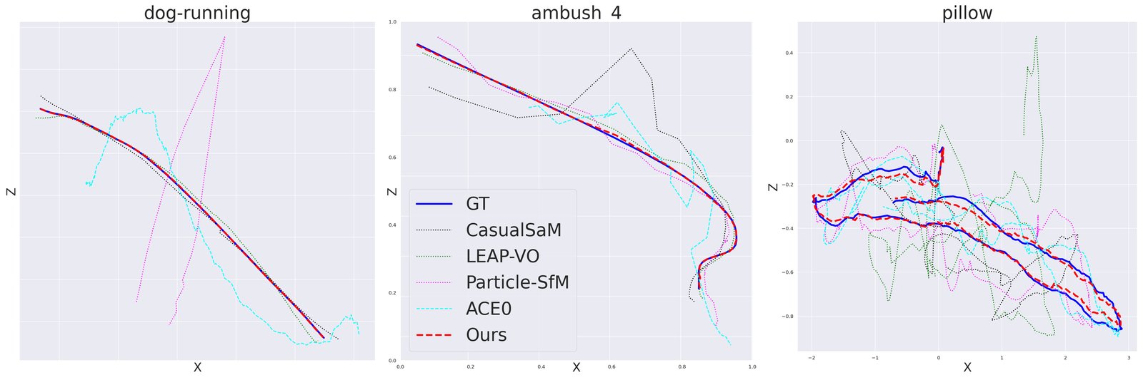
Sintel [4]	Dycheck [12]	In-the-Wild [32]

Figure 5: Visualization of estimated camera trajectories. Due to scene dynamics, our camera estimate (red dash) deviates less from the ground truth camera trajectory (blue solid line) than all other baselines.

Sintel [4]	Dycheck [12]	In-the-Wild [32]

图 5：估计相机轨迹可视化。由于场景动态，我们的相机估计（红色虚线）相对真值相机轨迹（蓝色实线）的偏离小于所有其他基线。

Metrics. We use standard error metrics to evaluate camera pose estimation: Absolute Translation Error (ATE), Relative Translation Error (RTE), and Relative Rotation Error (RRE). Following CasualSaM, we normalize ground truth camera trajectories to be unit length, since camera tracks in different videos can vary significantly, and videos with longer trajectories can have higher influence on the computed metrics. For all methods, we align estimated camera paths to the ground truth trajectory by computing a global $\mathrm{Sim}(3)$ transformation via Umeyama alignment [62]. We report the average running time by dividing total running time of each method by the number of input frames. Additionally, we compare the quality of estimated video depths to recent baselines, adopting standard depth metrics: Absolute Relative Error, log RMSE, and Delta accuracy. We follow the standard evaluation protocol by excluding points that are further than 100 meters. For all methods, we align predicted video depths with ground truth through a global scale and shift estimate.

指标。 相机位姿估计采用标准误差：绝对平移误差（ATE）、相对平移误差（RTE）与相对旋转误差（RRE）。按 CasualSaM，我们把真值相机轨迹归一化为单位长度，因为不同视频轨迹长度差异大，更长轨迹会对指标影响更大。对所有方法，经 Umeyama 对齐[62]计算全局 $\mathrm{Sim}(3)$ 变换，把估计相机路径对齐到真值轨迹。平均运行时间用各方法总时间除以输入帧数报告。另外，我们用标准深度指标比较估计视频深度质量：绝对相对误差、log RMSE 与 Delta 精度。评测按惯例排除超过 100 米的点。对所有方法，通过全局尺度与平移估计把预测视频深度对齐到真值。

4.2 Quantitative Comparisons

4.2 定量比较

Numerical results for camera pose estimation on the three benchmarks are reported in Tables 1, 2, and 3. Our approach demonstrates significant improvement and achieves the best camera tracking accuracy on all error metrics in both the calibrated and uncalibrated setting, while being competitive in terms of running time. Notably, our approach outperforms the concurrent work MonST3R [76] in terms of both robustness and accuracy even though MonST3R adopts a more recent global 3D point cloud representation for dynamic scenes. In addition, we report results for depth prediction on the Sintel and Dycheck in Table 4. Our depth estimates again outperform other baselines significantly in all metrics.

三个基准上的相机位姿数值结果见表 1、2、3。我们的方法在已标定与未标定设定下各项误差指标均取得最佳相机跟踪精度，相对先前工作提升明显，运行时间也具竞争力。值得注意的是，即便同期 MonST3R[76] 为动态场景采用了更新的全局三维点云表示，我们在鲁棒性与精度上仍更优。此外，表 4 报告了 Sintel 与 Dycheck 上的深度预测结果，我们的深度估计在全部指标上再次显著优于其他基线。

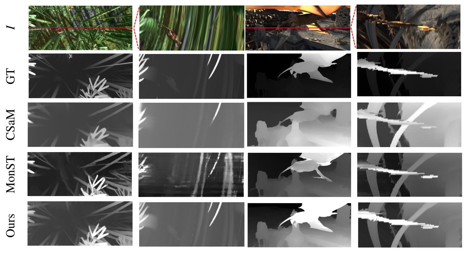
Figure 6: Visual comparisons of video depths. We compare video depth estimates from our approach and from CasualSAM [78] and MonST3R [76] by visualizing their depth maps (odd columns) and corresponding $x$-$t$ slices (even columns).

图 6：视频深度视觉比较。我们比较本方法与 CasualSAM[78]、MonST3R[76] 的视频深度估计，可视化深度图（奇数列）与对应 $x$-$t$ 切片（偶数列）。

	Poses	Depth
Method	ATE	RTE	RRE	Abs-Rel	$\delta_{1.25}$
Droid-SLAM [59]	0.030	0.022	0.50	-	-
w/o mono-init.	0.038	0.026	0.49	-	-
w/o $\hat{m}_{i}$	0.032	0.127	0.14	-	-
w/o 2-stage train.	0.035	0.136	0.17	-	-
w/o u-BA	0.033	0.013	0.11	-	-
w/ ft-pose	0.041	0.018	0.33	0.23	71.2
w/o new $\mathcal{C}_{\text{prior}}$	-	-	-	0.36	72.5
Full	0.019	0.008	0.04	0.21	73.1

Table 5: Ablation study on the Sintel dataset. Sec. 4.3 describes each configuration.

	位姿	深度
方法	ATE	RTE	RRE	Abs-Rel	$\delta_{1.25}$
Droid-SLAM [59]	0.030	0.022	0.50	-	-
w/o mono-init.	0.038	0.026	0.49	-	-
w/o $\hat{m}_{i}$	0.032	0.127	0.14	-	-
w/o 2-stage train.	0.035	0.136	0.17	-	-
w/o u-BA	0.033	0.013	0.11	-	-
w/ ft-pose	0.041	0.018	0.33	0.23	71.2
w/o new $\mathcal{C}_{\text{prior}}$	-	-	-	0.36	72.5
Full	0.019	0.008	0.04	0.21	73.1

表 5：Sintel 数据集上的消融研究。 第 4.3 节说明各配置。

4.3 Ablation study

4.3 消融研究

We perform an ablation study to validate major design choices for our camera tracking and depth estimation modules. Specifically, we evaluate camera tracking results with different configurations: 1) vanilla Droid-SLAM [59], 2) without mono-depth initialization (w/o mono-init.), 3) without object movement map prediction (w/o $\hat{m}_{i}$), 4) directly train the model on dynamic videos without using proposed two-stage training scheme (w/o 2-stage train.), 5) always turn on mono-depth regularization during global BA (w/o u-BA). We also ablate two major design decisions for video depth estimation: 1) jointly refine camera poses and depth estimation (w/o ft-pose), and 2) use original mono-depth prior loss from CasualSAM instead of our proposed one (w/o new $\mathcal{C}_{prior}$). As shown in Table 5, our full system outperforms all other alternative configurations.

我们做消融以验证相机跟踪与深度估计模块的主要设计选择。相机跟踪比较如下配置：1) 原版 Droid-SLAM[59]；2) 无单目深度初始化（w/o mono-init.）；3) 无物体运动图预测（w/o $\hat{m}_{i}$）；4) 不采用所提两阶段训练、直接在动态视频上训练（w/o 2-stage train.）；5) 全局 BA 中始终打开单目深度正则（w/o u-BA）。视频深度估计另消融两项：1) 联合精炼相机位姿与深度（w/ ft-pose）；2) 使用 CasualSAM 原始单目深度先验损失而非我们提出的版本（w/o new $\mathcal{C}_{prior}$）。如表 5 所示，完整系统优于所有替代配置。

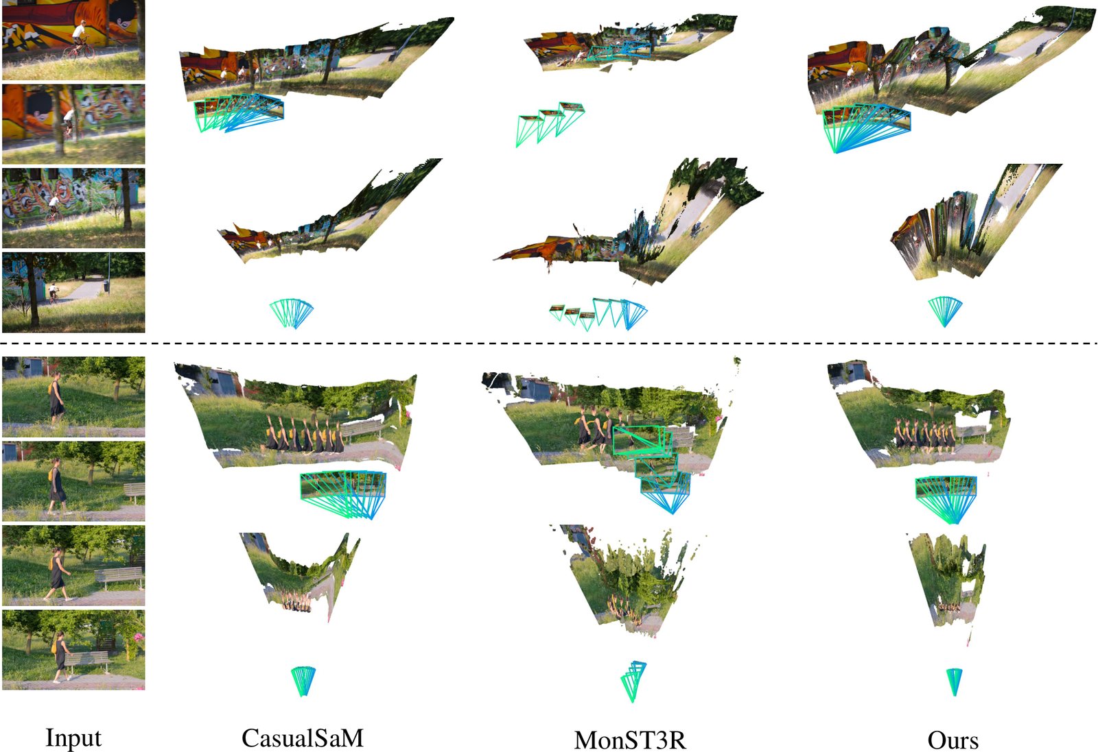
Figure 7: We visualize two examples from DAVIS with rotation-dominant camera motion and narrow FoV. Compared to CasualSAM [78] and MonST3R [76], our system produces more accurate camera and geometry estimates of underlying dynamic scenes.

图 7：我们可视化 DAVIS 上两例旋转主导相机运动且视场较窄的结果。相对 CasualSAM[78] 与 MonST3R[76]，我们的系统对底层动态场景给出更准的相机与几何估计。

4.4 Qualitative Comparisons

4.4 定性比较

Fig. 5 shows qualitative comparisons of estimated camera trajectory from our method and other baselines in 2D on three benchmarks, and our camera estimates are the closest to the ground truth. Furthermore, we visualize and compare the estimated video depths from our approach and two recent optimization based techniques, CasualSAM [78] and MonST3R [76], in Fig 6. In particular, we visualize both the depth map of a reference frame and corresponding $x$-$t$ depth slices over the entire video. Our approach once again produces more accurate, detailed and temporally consistent video depths.

图 5 在三个基准上以二维展示本方法与其他基线估计相机轨迹的定性比较，我们的相机估计最接近真值。进而，图 6 可视化并比较本方法与两种近期基于优化的技术 CasualSAM[78]、MonST3R[76] 的估计视频深度：展示参考帧深度图以及整段视频上对应的 $x$-$t$ 深度切片。本方法再次给出更准、更细、时间上更一致的视频深度。

Last, we compare reconstruction and camera tracking quality among different approaches on challenging examples from DAVIS [42] by visualizing their estimated cameras and unprojected depth maps. As shown in Fig. 7, CasualSaM tends to produce distorted 3D point clouds, whereas MonST3R incorrectly treats rotational camera movement as translational one. In contrast, our approach produces more accurate camera along with more consistent geometry for such challenging inputs.

最后，我们在 DAVIS[42] 的困难样例上，通过可视化估计相机与反投影深度图，比较不同方法的重建与相机跟踪质量。如图 7，CasualSaM 往往产生扭曲的三维点云，而 MonST3R 会把旋转相机运动误当成平移。相比之下，本方法对此类困难输入给出更准的相机与更一致的几何。

5 Discussion and conclusion

5 讨论与结论

Limitations.

Despite excellent performance on a variety of in-the-wild videos, we observe that our approach can fail in extremely challenging scenarios, similar to findings from prior work [78]. For instance, camera tracking fails if moving objects dominate the entire image or if there is nothing for the system to track reliably. Please see supplemental material for visualization of failure cases. Furthermore, our system cannot handle videos with varying focal lengths or strong radial distortion within the video. Incorporating better priors from current vision foundation models into the pipelines is a promising future direction to explore.

局限。

尽管在各类野外视频上表现优异，我们观察到在极端困难场景下方法仍可能失败，这与先前工作[78]的发现类似。例如，若运动物体占据整幅图像，或场景中几乎没有可可靠跟踪的内容，相机跟踪就会失败。失败样例可视化见补充材料。此外，系统无法处理视频内焦距变化或强径向畸变。把当前视觉基础模型中更好的先验接入管线，是有前景的未来方向。

Conclusion.

We presented a pipeline that produces accurate camera parameters and consistent depths from casual monocular videos of dynamic scenes. Our approach efficiently scales to in-the-wild footage of varying time duration, with unconstrained camera paths and complex scene dynamics. We have shown that, with careful extension, prior deep visual SLAM and SfM frameworks can be extended to achieve strong generalization to a broad range of videos and outperform recent state-of-the-art methods significantly.

结论。

我们提出一条管线，能从日常动态场景单目视频得到准确相机参数与一致深度。方法高效扩展到时长各异、相机路径不受限、场景动态复杂的野外素材。结果表明，经仔细扩展，先前深度视觉 SLAM 与 SfM 框架可泛化到更广的视频范围，并显著优于近期先进方法。

References

参考文献

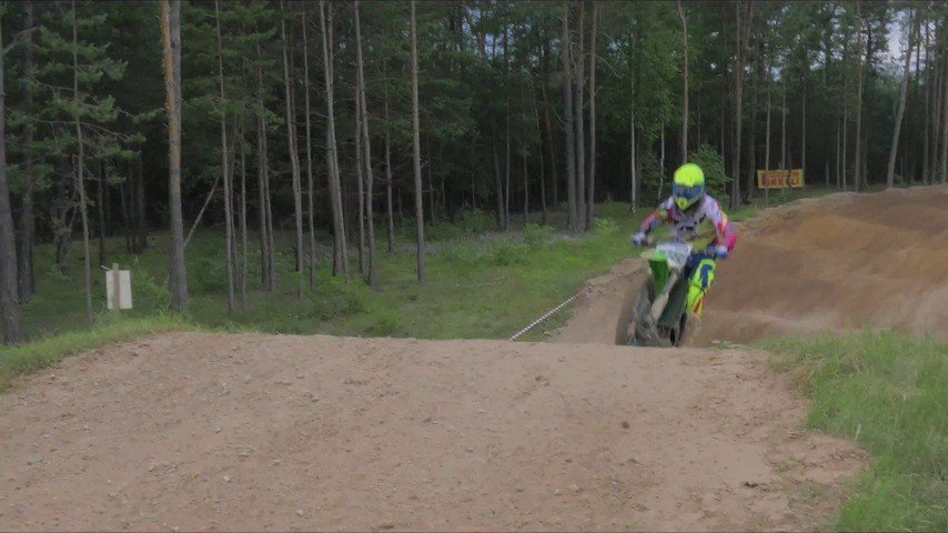
Figure 8: Limitations. We visualize three reference video frames on the left and their corresponding estimated camera paths and reconstruction on the right. Our method can lose tracks in cases where a moving object dominates the entire videos (top row). Our approach can also struggle in cases where object motion and camera motion are colinear, such as the selfie video in the bottom row.

图 8：局限。 左列可视化三帧参考视频，右列是对应估计的相机路径与重建。当运动物体主导整段视频时，方法可能丢跟踪（上行）。物体运动与相机运动共线时也会吃力，如下行自拍视频。

[1] Sameer Agarwal, Yasutaka Furukawa, Noah Snavely, Ian Simon, Brian Curless, Steven M Seitz, and Richard Szeliski. Building rome in a day. Communications of the ACM , 54(10):105–112, 2011.

[2] Michael Bloesch, Jan Czarnowski, Ronald Clark, Stefan Leutenegger, and Andrew J Davison. Codeslam—learning a compact, optimisable representation for dense visual slam. In Proceedings of the IEEE conference on computer vision and pattern recognition , pages 2560–2568, 2018.

[3] Eric Brachmann, Jamie Wynn, Shuai Chen, Tommaso Cavallari, Áron Monszpart, Daniyar Turmukhambetov, and Victor Adrian Prisacariu. Scene coordinate reconstruction: Posing of image collections via incremental learning of a relocalizer. arXiv preprint arXiv:2404.14351 , 2024.

[4] D. J. Butler, J. Wulff, G. B. Stanley, and M. J. Black. A naturalistic open source movie for optical flow evaluation. In European Conf. on Computer Vision (ECCV) , pages 611–625. Springer-Verlag, 2012.

[5] Carlos Campos, Richard Elvira, Juan J Gómez Rodríguez, José MM Montiel, and Juan D Tardós. Orb-slam3: An accurate open-source library for visual, visual–inertial, and multimap slam. IEEE Transactions on Robotics , 37(6):1874–1890, 2021.

[6] Weirong Chen, Le Chen, Rui Wang, and Marc Pollefeys. Leap-vo: Long-term effective any point tracking for visual odometry. In Proc. Computer Vision and Pattern Recognition (CVPR) , pages 19844–19853, 2024.

[7] Jan Czarnowski, Tristan Laidlow, Ronald Clark, and Andrew J Davison. Deepfactors: Real-time probabilistic dense monocular slam. IEEE Robotics and Automation Letters , 5(2):721–728, 2020.

[8] Andrew J Davison, Ian D Reid, Nicholas D Molton, and Olivier Stasse. Monoslam: Real-time single camera slam. IEEE transactions on pattern analysis and machine intelligence , 29(6):1052–1067, 2007.

[9] Jakob Engel, Thomas Schöps, and Daniel Cremers. Lsd-slam: Large-scale direct monocular slam. In European conference on computer vision , pages 834–849. Springer, 2014.

[10] Jakob Engel, Vladlen Koltun, and Daniel Cremers. Direct sparse odometry. IEEE transactions on pattern analysis and machine intelligence , 40(3):611–625, 2017.

[11] Yang Fu, Sifei Liu, Amey Kulkarni, Jan Kautz, Alexei A. Efros, and Xiaolong Wang. Colmap-free 3d gaussian splatting. In Proc. Computer Vision and Pattern Recognition (CVPR) , pages 20796–20805, 2024.

[12] Hang Gao, Ruilong Li, Shubham Tulsiani, Bryan Russell, and Angjoo Kanazawa. Monocular dynamic view synthesis: A reality check. Advances in Neural Information Processing Systems , 35:33768–33780, 2022.

[13] Clément Godard, Oisin Mac Aodha, and Gabriel J Brostow. Unsupervised monocular depth estimation with left-right consistency. In Proceedings of the IEEE conference on computer vision and pattern recognition , pages 270–279, 2017.

[14] Lily Goli, Cody Reading, Silvia Sellán, Alec Jacobson, and Andrea Tagliasacchi. Bayes’ rays: Uncertainty quantification for neural radiance fields. In Proc. Computer Vision and Pattern Recognition (CVPR) , pages 20061–20070, 2024.

[15] Klaus Greff, Francois Belletti, Lucas Beyer, Carl Doersch, Yilun Du, Daniel Duckworth, David J Fleet, Dan Gnanapragasam, Florian Golemo, Charles Herrmann, Thomas Kipf, Abhijit Kundu, Dmitry Lagun, Issam Laradji, Hsueh-Ti (Derek) Liu, Henning Meyer, Yishu Miao, Derek Nowrouzezahrai, Cengiz Oztireli, Etienne Pot, Noha Radwan, Daniel Rebain, Sara Sabour, Mehdi S. M. Sajjadi, Matan Sela, Vincent Sitzmann, Austin Stone, Deqing Sun, Suhani Vora, Ziyu Wang, Tianhao Wu, Kwang Moo Yi, Fangcheng Zhong, and Andrea Tagliasacchi. Kubric: a scalable dataset generator. 2022.

[16] Annika Hagemann, Moritz Knorr, and Christoph Stiller. Deep geometry-aware camera self-calibration from video. In Proceedings of the IEEE/CVF International Conference on Computer Vision , pages 3438–3448, 2023.

[17] Kaiming He, Georgia Gkioxari, Piotr Dollár, and Ross Girshick. Mask r-cnn. In Proceedings of the IEEE international conference on computer vision , pages 2961–2969, 2017.

[18] Xingyi He, Jiaming Sun, Yifan Wang, Sida Peng, Qixing Huang, Hujun Bao, and Xiaowei Zhou. Detector-free structure from motion. In Proceedings of the IEEE/CVF Conference on Computer Vision and Pattern Recognition , pages 21594–21603, 2024.

[19] Aleksander Holynski, David Geraghty, Jan-Michael Frahm, Chris Sweeney, and Richard Szeliski. Reducing drift in structure from motion using extended features. In 2020 International Conference on 3D Vision (3DV) , pages 51–60. IEEE, 2020.

[20] Wenbo Hu, Xiangjun Gao, Xiaoyu Li, Sijie Zhao, Xiaodong Cun, Yong Zhang, Long Quan, and Ying Shan. Depthcrafter: Generating consistent long depth sequences for open-world videos. arXiv preprint arXiv:2409.02095 , 2024.

[21] Yoni Kasten, Wuyue Lu, and Haggai Maron. Fast encoder-based 3d from casual videos via point track processing. In The Thirty-eighth Annual Conference on Neural Information Processing Systems .

[22] Bingxin Ke, Anton Obukhov, Shengyu Huang, Nando Metzger, Rodrigo Caye Daudt, and Konrad Schindler. Repurposing diffusion-based image generators for monocular depth estimation. In Proceedings of the IEEE/CVF Conference on Computer Vision and Pattern Recognition , pages 9492–9502, 2024.

[23] Alex Kendall and Yarin Gal. What uncertainties do we need in bayesian deep learning for computer vision? Advances in neural information processing systems , 30, 2017.

[24] Diederik P. Kingma and Jimmy Ba. Adam: A method for stochastic optimization. CoRR , abs/1412.6980, 2014.

[25] Georg Klein and David Murray. Parallel tracking and mapping for small ar workspaces. In 2007 6th IEEE and ACM international symposium on mixed and augmented reality , pages 225–234. IEEE, 2007.

[26] Johannes Kopf, Xuejian Rong, and Jia-Bin Huang. Robust consistent video depth estimation. In Proc. Computer Vision and Pattern Recognition (CVPR) , 2021.

[27] Jiahui Lei, Yijia Weng, Adam Harley, Leonidas Guibas, and Kostas Daniilidis. Mosca: Dynamic gaussian fusion from casual videos via 4d motion scaffolds. arXiv preprint arXiv:2405.17421 , 2024.

[28] Vincent Leroy, Yohann Cabon, and Jérôme Revaud. Grounding image matching in 3d with mast3r. arXiv preprint arXiv:2406.09756 , 2024.

[29] Zhengqi Li and Noah Snavely. Megadepth: Learning single-view depth prediction from internet photos. In Proceedings of the IEEE conference on computer vision and pattern recognition , pages 2041–2050, 2018.

[30] Zhengqi Li, Tali Dekel, Forrester Cole, Richard Tucker, Noah Snavely, Ce Liu, and William T Freeman. Learning the depths of moving people by watching frozen people. In Proc. Computer Vision and Pattern Recognition (CVPR) , pages 4521–4530, 2019.

[31] Zhengqi Li, Simon Niklaus, Noah Snavely, and Oliver Wang. Neural scene flow fields for space-time view synthesis of dynamic scenes. In Proceedings of the IEEE/CVF Conference on Computer Vision and Pattern Recognition , pages 6498–6508, 2021.

[32] Zhengqi Li, Qianqian Wang, Forrester Cole, Richard Tucker, and Noah Snavely. Dynibar: Neural dynamic image-based rendering. In Proc. Computer Vision and Pattern Recognition (CVPR) , pages 4273–4284, 2023.

[33] Chen-Hsuan Lin, Wei-Chiu Ma, Antonio Torralba, and Simon Lucey. Barf: Bundle-adjusting neural radiance fields. In Proc. Computer Vision and Pattern Recognition (CVPR) , pages 5741–5751, 2021.

[34] Yu-Lun Liu, Chen Gao, Andreas Meuleman, Hung-Yu Tseng, Ayush Saraf, Changil Kim, Yung-Yu Chuang, Johannes Kopf, and Jia-Bin Huang. Robust dynamic radiance fields. In Proc. Computer Vision and Pattern Recognition (CVPR) , pages 13–23, 2023.

[35] Xuan Luo, Jia-Bin Huang, Richard Szeliski, Kevin Matzen, and Johannes Kopf. Consistent video depth estimation. ACM Transactions on Graphics (ToG) , 39(4):71–1, 2020.

[36] Thomas Müller, Alex Evans, Christoph Schied, and Alexander Keller. Instant neural graphics primitives with a multiresolution hash encoding. ACM Trans. Graph. , 41(4):102:1–102:15, 2022.

[37] Raul Mur-Artal, Jose Maria Martinez Montiel, and Juan D Tardos. Orb-slam: a versatile and accurate monocular slam system. IEEE transactions on robotics , 31(5):1147–1163, 2015.

[38] Richard A Newcombe, Steven J Lovegrove, and Andrew J Davison. Dtam: Dense tracking and mapping in real-time. In Proc. Int. Conf. on Computer Vision (ICCV) , pages 2320–2327. IEEE, 2011.

[39] Keunhong Park, Utkarsh Sinha, Jonathan T Barron, Sofien Bouaziz, Dan B Goldman, Steven M Seitz, and Ricardo Martin-Brualla. Nerfies: Deformable neural radiance fields. In Proc. Computer Vision and Pattern Recognition (CVPR) , pages 5865–5874, 2021a.

[40] Keunhong Park, Utkarsh Sinha, Peter Hedman, Jonathan T Barron, Sofien Bouaziz, Dan B Goldman, Ricardo Martin-Brualla, and Steven M Seitz. Hypernerf: A higher-dimensional representation for topologically varying neural radiance fields. arXiv preprint arXiv:2106.13228 , 2021b.

[41] Keunhong Park, Philipp Henzler, Ben Mildenhall, Jonathan T Barron, and Ricardo Martin-Brualla. Camp: Camera preconditioning for neural radiance fields. ACM Transactions on Graphics (TOG) , 42(6):1–11, 2023.

[42] F. Perazzi, J. Pont-Tuset, B. McWilliams, L. Van Gool, M. Gross, and A. Sorkine-Hornung. A benchmark dataset and evaluation methodology for video object segmentation. In Computer Vision and Pattern Recognition , 2016.

[43] Luigi Piccinelli, Yung-Hsu Yang, Christos Sakaridis, Mattia Segu, Siyuan Li, Luc Van Gool, and Fisher Yu. UniDepth: Universal monocular metric depth estimation. In Proc. Computer Vision and Pattern Recognition (CVPR) , 2024.

[44] Marc Pollefeys, Luc Van Gool, Maarten Vergauwen, Frank Verbiest, Kurt Cornelis, Jan Tops, and Reinhard Koch. Visual modeling with a hand-held camera. International Journal of Computer Vision , 59:207–232, 2004.

[45] Marc Pollefeys, David Nistér, J-M Frahm, Amir Akbarzadeh, Philippos Mordohai, Brian Clipp, Chris Engels, David Gallup, S-J Kim, Paul Merrell, et al. Detailed real-time urban 3d reconstruction from video. International Journal of Computer Vision , 78:143–167, 2008.

[46] René Ranftl, Katrin Lasinger, David Hafner, Konrad Schindler, and Vladlen Koltun. Towards robust monocular depth estimation: Mixing datasets for zero-shot cross-dataset transfer. IEEE transactions on pattern analysis and machine intelligence , 44(3):1623–1637, 2020.

[47] René Ranftl, Alexey Bochkovskiy, and Vladlen Koltun. Vision transformers for dense prediction. In Proc. Computer Vision and Pattern Recognition (CVPR) , pages 12179–12188, 2021.

[48] Hippolyt Ritter, Aleksandar Botev, and David Barber. A scalable laplace approximation for neural networks. In 6th international conference on learning representations, ICLR 2018-conference track proceedings . International Conference on Representation Learning, 2018.

[49] Saurabh Saxena, Charles Herrmann, Junhwa Hur, Abhishek Kar, Mohammad Norouzi, Deqing Sun, and David J Fleet. The surprising effectiveness of diffusion models for optical flow and monocular depth estimation. Advances in Neural Information Processing Systems , 36, 2024.

[50] Mohamed Sayed, John Gibson, Jamie Watson, Victor Prisacariu, Michael Firman, and Clément Godard. Simplerecon: 3d reconstruction without 3d convolutions. In European Conference on Computer Vision , pages 1–19. Springer, 2022.

[51] Johannes L Schonberger and Jan-Michael Frahm. Structure-from-motion revisited. In Proceedings of the IEEE conference on computer vision and pattern recognition , pages 4104–4113, 2016.

[52] Johannes L Schönberger, Enliang Zheng, Jan-Michael Frahm, and Marc Pollefeys. Pixelwise view selection for unstructured multi-view stereo. In Computer Vision–ECCV 2016: 14th European Conference, Amsterdam, The Netherlands, October 11-14, 2016, Proceedings, Part III 14 , pages 501–518. Springer, 2016.

[53] Jiahao Shao, Yuanbo Yang, Hongyu Zhou, Youmin Zhang, Yujun Shen, Matteo Poggi, and Yiyi Liao. Learning temporally consistent video depth from video diffusion priors. arXiv preprint arXiv:2406.01493 , 2024.

[54] Shihao Shen, Yilin Cai, Wenshan Wang, and Sebastian Scherer. Dytanvo: Joint refinement of visual odometry and motion segmentation in dynamic environments. In 2023 IEEE International Conference on Robotics and Automation (ICRA) , pages 4048–4055. IEEE, 2023.

[55] Noah Snavely, Steven M Seitz, and Richard Szeliski. Photo tourism: exploring photo collections in 3d. In ACM siggraph 2006 papers , pages 835–846. 2006.

[56] Chris Sweeney, Aleksander Holynski, Brian Curless, and Steve M Seitz. Structure from motion for panorama-style videos. arXiv preprint arXiv:1906.03539 , 2019.

[57] Chengzhou Tang and Ping Tan. Ba-net: Dense bundle adjustment network. arXiv preprint arXiv:1806.04807 , 2018.

[58] Zachary Teed and Jia Deng. Raft: Recurrent all-pairs field transforms for optical flow. In Computer Vision–ECCV 2020: 16th European Conference, Glasgow, UK, August 23–28, 2020, Proceedings, Part II 16 , pages 402–419. Springer, 2020.

[59] Zachary Teed and Jia Deng. Droid-slam: Deep visual slam for monocular, stereo, and rgb-d cameras. Advances in neural information processing systems , 34:16558–16569, 2021.

[60] Zachary Teed, Lahav Lipson, and Jia Deng. Deep patch visual odometry. Advances in Neural Information Processing Systems , 36, 2024.

[61] Bill Triggs, Philip F McLauchlan, Richard I Hartley, and Andrew W Fitzgibbon. Bundle adjustment—a modern synthesis. In Vision Algorithms: Theory and Practice: International Workshop on Vision Algorithms Corfu, Greece, September 21–22, 1999 Proceedings , pages 298–372. Springer, 2000.

[62] Shinji Umeyama. Least-squares estimation of transformation parameters between two point patterns. IEEE Transactions on Pattern Analysis & Machine Intelligence , 13(04):376–380, 1991.

[63] Jianyuan Wang, Nikita Karaev, Christian Rupprecht, and David Novotny. Vggsfm: Visual geometry grounded deep structure from motion. In Proceedings of the IEEE/CVF Conference on Computer Vision and Pattern Recognition , pages 21686–21697, 2024a.

[64] Qianqian Wang, Vickie Ye, Hang Gao, Jake Austin, Zhengqi Li, and Angjoo Kanazawa. Shape of motion: 4d reconstruction from a single video. arXiv preprint arXiv:2407.13764 , 2024b.

[65] Sen Wang, Ronald Clark, Hongkai Wen, and Niki Trigoni. Deepvo: Towards end-to-end visual odometry with deep recurrent convolutional neural networks. In 2017 IEEE international conference on robotics and automation (ICRA) , pages 2043–2050. IEEE, 2017.

[66] Shuzhe Wang, Vincent Leroy, Yohann Cabon, Boris Chidlovskii, and Jerome Revaud. Dust3r: Geometric 3d vision made easy. In Proc. Computer Vision and Pattern Recognition (CVPR) , pages 20697–20709, 2024c.

[67] Shizun Wang, Xingyi Yang, Qiuhong Shen, Zhenxiang Jiang, and Xinchao Wang. Gflow: Recovering 4d world from monocular video. arXiv preprint arXiv:2405.18426 , 2024d.

[68] Wenshan Wang, Delong Zhu, Xiangwei Wang, Yaoyu Hu, Yuheng Qiu, Chen Wang, Yafei Hu, Ashish Kapoor, and Sebastian Scherer. Tartanair: A dataset to push the limits of visual slam. 2020.

[69] Yiran Wang, Min Shi, Jiaqi Li, Zihao Huang, Zhiguo Cao, Jianming Zhang, Ke Xian, and Guosheng Lin. Neural video depth stabilizer. In Proc. Computer Vision and Pattern Recognition (CVPR) , pages 9466–9476, 2023.

[70] Rundi Wu, Ruiqi Gao, Ben Poole, Alex Trevithick, Changxi Zheng, Jonathan T Barron, and Aleksander Holynski. Cat4d: Create anything in 4d with multi-view video diffusion models. arXiv preprint arXiv:2411.18613 , 2024.

[71] Lihe Yang, Bingyi Kang, Zilong Huang, Xiaogang Xu, Jiashi Feng, and Hengshuang Zhao. Depth anything: Unleashing the power of large-scale unlabeled data. In CVPR , 2024a.

[72] Lihe Yang, Bingyi Kang, Zilong Huang, Zhen Zhao, Xiaogang Xu, Jiashi Feng, and Hengshuang Zhao. Depth anything v2. arXiv preprint arXiv:2406.09414 , 2024b.

[73] Nan Yang, Lukas von Stumberg, Rui Wang, and Daniel Cremers. D3vo: Deep depth, deep pose and deep uncertainty for monocular visual odometry. In Proc. Computer Vision and Pattern Recognition (CVPR) , pages 1281–1292, 2020.

[74] Wei Yin, Jianming Zhang, Oliver Wang, Simon Niklaus, Long Mai, Simon Chen, and Chunhua Shen. Learning to recover 3d scene shape from a single image. In Proc. Computer Vision and Pattern Recognition (CVPR) , pages 204–213, 2021.

[75] Wei Yin, Chi Zhang, Hao Chen, Zhipeng Cai, Gang Yu, Kaixuan Wang, Xiaozhi Chen, and Chunhua Shen. Metric3d: Towards zero-shot metric 3d prediction from a single image. In Proc. Computer Vision and Pattern Recognition (CVPR) , pages 9043–9053, 2023.

[76] Junyi Zhang, Charles Herrmann, Junhwa Hur, Varun Jampani, Trevor Darrell, Forrester Cole, Deqing Sun, and Ming-Hsuan Yang. MonST3R: A simple approach for estimating geometry in the presence of motion. arXiv preprint arXiv:2410.03825 , 2024.

[77] Zhoutong Zhang, Forrester Cole, Richard Tucker, William T Freeman, and Tali Dekel. Consistent depth of moving objects in video. ACM Transactions on Graphics (ToG) , 40(4):1–12, 2021.

[78] Zhoutong Zhang, Forrester Cole, Zhengqi Li, Michael Rubinstein, Noah Snavely, and William T Freeman. Structure and motion from casual videos. In European Conference on Computer Vision , pages 20–37. Springer, 2022.

[79] Wang Zhao, Shaohui Liu, Hengkai Guo, Wenping Wang, and Yong-Jin Liu. Particlesfm: Exploiting dense point trajectories for localizing moving cameras in the wild. In European Conference on Computer Vision , pages 523–542. Springer, 2022.

Appendix A Implementation Details

附录 A 实现细节

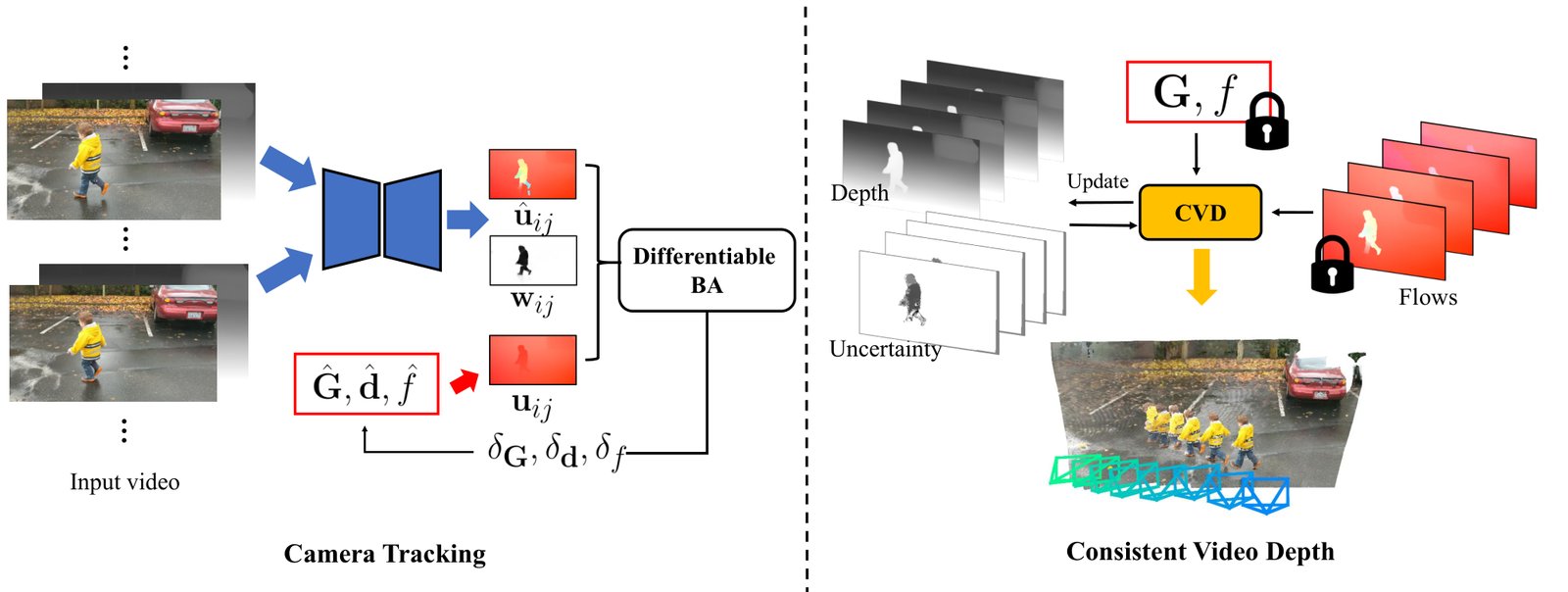
Figure 9: System overview. Left: we estimate camera poses, focal length and low-resolution disparity maps from the input monocular video through differentiable Bundle Adjustment (BA): the network iteratively updates these state variables by learning to predict low-resolution flow $\hat{\mathbf{u}}_{ij}$, confidence, and movement probability maps $\mathbf{w}_{ij}$ and minimize weighted reprojection error between predicted flow ${\hat{\mathbf{u}}}_{ij}$ and flow induced by ego-motion ${\mathbf{u}}_{ij}$. We also initialize estimated disparity with mono-depth predicted from off-the-shelf models [71, 43]. Right: we fix estimated camera parameters and perform first-order global optimization over video depth and corresponding uncertainty parameters by minimizing flow and depth losses through pairwise 2D optical flows.

图 9：系统总览。左：经可微光束法平差（BA）从输入单目视频估计相机位姿、焦距与低分辨率视差图：网络迭代更新这些状态变量，学习预测低分辨率光流 $\hat{\mathbf{u}}_{ij}$、置信度与运动概率图 $\mathbf{w}_{ij}$，并最小化预测光流 ${\hat{\mathbf{u}}}_{ij}$ 与自运动诱导光流 ${\mathbf{u}}_{ij}$ 之间的加权重投影误差。估计视差还用现成模型[71, 43]预测的单目深度做初始化。右：固定已估相机参数，对视频深度及对应不确定性参数做一阶全局优化，借助成对二维光流最小化光流与深度损失。

A.1 System Overview

A.1 系统总览

Figure 9 shows an overview of our MegaSaM system. We separate the problem of camera and scene structure estimation into two stages, in the spirit of a conventional SfM pipeline [51, 52]. In particular, we first estimate camera poses $\hat{\mathbf{G}}$, focal length $\hat{f}$ and low-resolution disparity $\hat{\mathbf{d}}$ from the input monocular video through differentiable Bundle Adjustment (BA), where we initialize $\hat{\mathbf{d}}$ with monocular depth maps predicted from off-the-shelf models [71, 43]. In the second consistent video depth estimation phase, we fix estimated camera parameters and perform first-order optimization over video depth and uncertainty maps by enforcing flow and depth losses induced by pairwise 2D optical flows.

图 9 给出 MegaSaM 系统总览。我们按传统 SfM 管线[51, 52]的精神，把相机与场景结构估计拆成两阶段。具体地，先经可微光束法平差（BA）从输入单目视频估计相机位姿 $\hat{\mathbf{G}}$、焦距 $\hat{f}$ 与低分辨率视差 $\hat{\mathbf{d}}$，其中 $\hat{\mathbf{d}}$ 用现成模型[71, 43]预测的单目深度图初始化。第二阶段一致视频深度估计中，固定已估相机参数，通过对成对二维光流施加光流与深度损失，对视频深度与不确定性图做一阶优化。

A.2 Framework and Architecture

A.2 框架与架构

We follow DROID-SLAM [58] for feature extraction, correlation feature construction, and perform iterative BA updates through flow, confidence, motion probability predictions. Each input to the model is a pair of video frames $(I_{i},I_{j})$.

特征提取、相关特征构造以及经光流、置信度、运动概率预测的迭代 BA 更新，我们遵循 DROID-SLAM[58]。模型每次输入一对视频帧 $(I_{i},I_{j})$。

Feature extraction. We use context and feature encoders to encode each input video frame into two different low-resolution feature maps at $\frac{1}{8}$ resolution of the input image, as shown in Figure 11.

特征提取。 我们用上下文编码器与特征编码器把每帧编码为输入图像 $\frac{1}{8}$ 分辨率的两路低分辨率特征图，见图 11。

Correlation feature construction. The correlation layer constructs a 4D correlation volume from the features encoded from an image pair, and each entry of the volume contains inner product of one pairs of feature vectors from the image pair.

相关特征构造。 相关层从图像对编码特征构造四维相关体，体中每个条目是图像对中一对特征向量的内积。

Iterative updates. During each iterative BA step $k$, we update camera parameters and low-resolution disparity through flow, confidence and motion probability prediction. In particular, we first pretrain $F$ on synthetic video data (ego-motion pretraining in the main paper) to learn to predict flows and corresponding flow confidence, as shown by the gray blocks in Figure 10. In the second dynamic finetuning phase, we freeze the parameters of $F$ and finetune the motion module $F_{m}$ to predict extra object motion probability maps conditioned on the features from the ConvRGU, as shown in the blue blocks in Figure 10. Within the motion module, we first perform 2D spatial average pooling to provide the model with global spatial information; we then perform average pooling along the time axis to fuse information from $I_{i}$ and all its neighboring keyframes $I_{j}$ (where $j\in\mathcal{N}(i)$).

迭代更新。 每次迭代 BA 步 $k$ 中，我们通过光流、置信度与运动概率预测更新相机参数与低分辨率视差。具体地，先在合成视频数据上预训练 $F$（正文中的自运动预训练），学习预测光流及对应光流置信度，见图 10 灰色块。第二阶段动态微调中，冻结 $F$ 参数，微调运动模块 $F_{m}$，使其条件于 ConvGRU 特征以预测额外的物体运动概率图，见图 10 蓝色块。运动模块内先做二维空间平均池化以提供全局空间信息，再沿时间轴平均池化，融合 $I_{i}$ 及其全部邻域关键帧 $I_{j}$（$j\in\mathcal{N}(i)$）的信息。

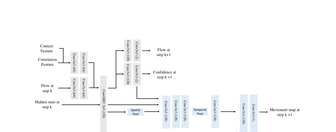
Figure 10: Architecture of flow, confidence and movement map predictor. The gray blocks belong to the network $F$ for flow and confidence prediction, and the blue blocks belong to the network $F_{m}$ for object movement map prediction. In the first stage, we perform ego-motion pretraining for $F$. In the second stage, we perform dynamic fine-tuning for $F_{m}$ while fixing the parameters of $F$.

图 10：光流、置信度与运动图预测器架构。灰色块属于用于光流与置信度预测的网络 $F$，蓝色块属于用于物体运动图预测的网络 $F_{m}$。第一阶段对 $F$ 做自运动预训练；第二阶段固定 $F$ 参数，对 $F_{m}$ 做动态微调。

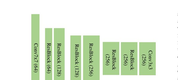
Figure 11: Architecture of the feature and context encoders. Both encoders extract low-resolution features from input video frames at $\frac{1}{8}$ of the original resolution.

图 11：特征与上下文编码器架构。两编码器均从输入视频帧提取原分辨率 $\frac{1}{8}$ 的低分辨率特征。

A.3 Consistent Video Depth Optimization

A.3 一致视频深度优化

Recall, from Section 3.3 of our main paper, that we follow CasualSAM [78] to estimate consistent video depth by performing an additional first-order optimization on video disparity $\hat{D}_{i}$ along with per-frame aleatoric uncertainty maps $\hat{M}_{i}$. Instead of jointly optimizing camera parameters and scene structure as in CasualSAM, however, we fix camera parameters as done in conventional SfM pipelines like COLMAP [51, 52].

回顾正文第 3.3 节：我们遵循 CasualSAM[78]，对视频视差 $\hat{D}_{i}$ 与每帧偶然不确定性图 $\hat{M}_{i}$ 再做一阶优化以估计一致视频深度。但与 CasualSAM 联合优化相机与场景结构不同，我们像 COLMAP[51, 52] 等传统 SfM 管线一样固定相机参数。

Our objective consists of three main cost functions:

目标由三项主要代价组成：

$$\mathcal{C}_{\text{cvd}}=w_{\text{flow}}\mathcal{C}_{\text{flow}}+w_{\text{temp}}\mathcal{C}_{\text{temp}}+w_{\text{prior}}\mathcal{C}_{\text{prior}} \tag{12}$$

We treat object motion in the video as the heteroscedastic aleatoric uncertainty of the flow reprojection and depth consistency error [23], and assume the underlying noise is Laplacian [73]. Specifically, for each selected pair $(I_{i},I_{j})$, flow reprojection loss $\mathcal{C}_{\text{flow}}$ compares $l_{1}$ loss weighted by the uncertainty $\hat{M}_{i}$ between flows $\text{flow}_{i\rightarrow j}$ from an off-the-shelf flow estimator [58] and the correspondences ${\mathbf{u}}_{ij}$ induced by our estimated camera motion and disparity through a multi-view constraint:

我们把视频中的物体运动视为光流重投影与深度一致性误差的异方差偶然不确定性[23]，并假设底层噪声为拉普拉斯[73]。具体地，对每个选定对 $(I_{i},I_{j})$，光流重投影损失 $\mathcal{C}_{\text{flow}}$ 比较现成光流估计器[58]给出的 $\text{flow}_{i\rightarrow j}$ 与由估计相机运动、视差经多视图约束诱导的对应 ${\mathbf{u}}_{ij}$ 之间、由不确定性 $\hat{M}_{i}$ 加权的 $l_{1}$ 损失：

$$\displaystyle\mathcal{C}^{i\rightarrow j}_{\text{flow}} \\ \displaystyle=\hat{M}_{i}||{\mathbf{u}}_{ij}-\mathbf{p}_{i},\text{flow}_{i\rightarrow j}(\mathbf{p}_{i})||_{1}+\log\left(\frac{1}{\hat{M}_{i}}\right), \\ \displaystyle{{\mathbf{u}}_{ij}} \\ \displaystyle=\pi\left(\hat{\mathbf{G}}_{ij}\circ\pi^{-1}(\mathbf{p}_{i},\hat{D}_{i},K^{-1}),K\right) \tag{13}$$

$\mathcal{C}_{\text{temp}}$ is an uncertainty weighted temporal depth loss that encourages pixel disparity to be temporally consistent according to estimated 2D optical flow:

$\mathcal{C}_{\text{temp}}$ 是不确定性加权的时间深度损失，鼓励像素视差按估计的二维光流在时间上保持一致：

$$\displaystyle\mathcal{C}^{i\rightarrow j}_{\text{temp}} \\ \displaystyle=\hat{M}_{i}\delta\left(\mathbf{P}^{i\rightarrow j}_{z},\hat{D}_{j}(\mathbf{p}+\text{flow}_{i\rightarrow j}(\mathbf{p}))\right)+\log\left(\frac{1}{\hat{M}_{i}}\right) \\ \displaystyle\delta(a,b) \\ \displaystyle=||\max(\frac{a}{b},\frac{b}{a})||_{1} \\ \displaystyle\mathbf{P}^{i\rightarrow j}_{z} \\ \displaystyle=\left(D_{i}(\mathbf{p})\mathbf{R}_{i\rightarrow j}\mathbf{K}^{-1}\mathbf{p}+\mathbf{t}_{i\rightarrow j}\right)_{[z]} \tag{15}$$

$\mathbf{R}_{i\rightarrow j}$ and $\mathbf{t}_{i\rightarrow j}$ are relative camera rotation and translation between $I_{i}$ and $I_{j}$; [z] is an operator that retrieve the third component of the 3D point vector (i.e. $z$ value).

$\mathbf{R}_{i\rightarrow j}$ 与 $\mathbf{t}_{i\rightarrow j}$ 是 $I_{i}$ 与 $I_{j}$ 之间的相对相机旋转与平移；[z] 算子取出三维点向量的第三分量（即 $z$ 值）。

$\mathcal{C}_{\text{prior}}$ is a depth prior loss that stops the final estimated video disparity from drifting too much from the initial estimate from the mono-depth network, and it consists of three losses:

$\mathcal{C}_{\text{prior}}$ 是深度先验损失，阻止最终估计视频视差相对单目深度网络初值漂得太远，由三项损失组成：

$$\displaystyle\mathcal{C}_{\text{prior}}=\mathcal{C}_{\text{si}}+w_{\text{grad}}\mathcal{C}_{\text{grad}}+w_{\text{normal}}\mathcal{C}_{\text{normal}} \tag{16}$$

The scale-invariant depth loss $\mathcal{C}_{\text{si}}$ computes the mean square error of the difference among all pairs between optimized log-disparity $\log\hat{D}_{i}$ and initial log-disparity from the metric-aligned mono-depth prediction $\log D_{i}^{\text{align}}$.

尺度不变深度损失 $\mathcal{C}_{\text{si}}$ 计算优化对数视差 $\log\hat{D}_{i}$ 与度量对齐单目深度预测的初始对数视差 $\log D_{i}^{\text{align}}$ 之间、所有像素对差分的均方误差。

$$\displaystyle\mathcal{C}_{\text{si}} \\ \displaystyle=\frac{1}{n}\sum_{(\mathbf{p})}(R(\mathbf{p}))^{2}-\frac{1}{n^{2}}\left(\sum_{(\mathbf{p})}R(\mathbf{p})\right)^{2} \\ \displaystyle R_{i} \\ \displaystyle=\log(\hat{D}_{i})-\log(D_{i}^{\text{align}}). \tag{17}$$

$\mathcal{C}_{\text{grad}}$ is a multi-scale scale-invariant gradient matching term [29], which computes $l_{1}$ difference between estimated log disparity gradients and initial log-disparity gradients

$\mathcal{C}_{\text{grad}}$ 是多尺度尺度不变梯度匹配项[29]，计算估计对数视差梯度与初始对数视差梯度之间的 $l_{1}$ 差

$$\displaystyle\mathcal{C}_{\text{grad}} \\ \displaystyle=\frac{1}{n}\sum_{s}w_{\nabla}^{s}(\mathbf{p})\sum_{\mathbf{p}}\left(|\nabla_{x}R^{s}(\mathbf{p})|+|\nabla_{y}R^{s}(\mathbf{p})|\right) \\ \displaystyle w_{\nabla}^{s}(\mathbf{p}) \\ \displaystyle=1-\exp\left(-\beta_{\nabla}(\nabla_{x}R^{s}(\mathbf{p})+\nabla_{y}R^{s}(\mathbf{p}))\right) \tag{18}$$

where $R^{s}(\mathbf{p})$ is log-depth difference map at pixel position $\mathbf{p}$ and scale $s$. In other words, we only apply multi-scale gradient matching loss to pixels where the current estimated disparity deviates significantly from the original mono-depth.

其中 $R^{s}(\mathbf{p})$ 是像素位置 $\mathbf{p}$、尺度 $s$ 上的对数深度差分图。换言之，仅当当前估计视差明显偏离原始单目深度时，才对该像素施加多尺度梯度匹配损失。

$\mathcal{C}_{\text{normal}}$ is a surface normal loss that encourages that normal $\hat{\mathbf{N}}(\mathbf{p})$ derived from estimated disparity to be close to the surface normal $\mathbf{N}^{\text{align}}$ derived from the initial metric-aligned monocular disparity:

$\mathcal{C}_{\text{normal}}$ 是表面法向损失，鼓励由估计视差导出的法向 $\hat{\mathbf{N}}(\mathbf{p})$ 接近由初始度量对齐单目视差导出的表面法向 $\mathbf{N}^{\text{align}}$：

$$\displaystyle\mathcal{C}_{\text{normal}}=\sum_{\mathbf{p}}1-\hat{\mathbf{N}}(\mathbf{p})\cdot\mathbf{N}^{\text{align}}(\mathbf{p}) \tag{19}$$

We set $w_{\text{grad}}=1,w_{\text{normal}}=4,\beta_{\nabla}=5$ throughout our experiments. We simply choose image pairs $(I_{i},I_{j})$ from a set of fixed intervals following prior work [78]: $j\in(i+1,i+2,i+4,i+8,i+15)$. During optimization, we initialize the disparity variables from the metric-aligned monocular depth by combining estimates from off-the-shelf modules as described in the main paper [71, 43], and we initialize the uncertainty map with object motion probability maps predicted from our camera tracking module. The optimization first conducts a “warm-up” phase for 100 steps by fixing the video disparity variables and optimizing the per-frame uncertainty map, per-frame scale, shift variables using the aforementioned losses. The disparity maps and uncertainty maps are then optimized together under the aforementioned losses for another 400 steps.

实验中始终设 $w_{\text{grad}}=1,w_{\text{normal}}=4,\beta_{\nabla}=5$。图像对 $(I_{i},I_{j})$ 按先前工作[78]从固定间隔集合选取：$j\in(i+1,i+2,i+4,i+8,i+15)$。优化时，视差变量用正文所述、结合现成模块[71, 43]的度量对齐单目深度初始化；不确定性图用相机跟踪模块预测的物体运动概率图初始化。优化先做 100 步「预热」：固定视频视差变量，用上述损失优化每帧不确定性图以及每帧尺度、平移变量；再把视差图与不确定性图在上述损失下联合优化 400 步。

A.4 Additional Details

A.4 其他细节

Training Losses. We supervise our network using a combination of pose loss and flow loss. The flow loss is applied to pairs of adjacent frames. We compute the optical flow induced by the predicted depth and poses and the flow induced by the ground truth depth and poses. The loss is taken to be the average l2 distance between the two flow fields.

训练损失。 我们用位姿损失与光流损失的组合监督网络。光流损失施加在相邻帧对上：计算由预测深度与位姿诱导的光流，以及由真值深度与位姿诱导的光流，损失取两光流场之间的平均 $l_2$ 距离。

Given a set of ground truth poses $\{\mathbf{T}_{i}\}_{i=1}^{N}$ and predicted poses $\{\mathbf{G}_{i}\}_{i=1}^{N}$, the pose loss is taken to be the distance between the ground truth and predicted poses, $\mathcal{L}_{pose}=\sum_{i}||\text{Log}_{SE(3)}(\mathbf{T}_{i}^{-1}\cdot\mathbf{G}_{i})||_{2}$. We apply the losses to the output of every BA iteration with exponentially increasing weight using $\gamma=0.9^{k}$, where $k$ indicates the $k^{th}$ BA iterations.

给定真值位姿集合 $\{\mathbf{T}_{i}\}_{i=1}^{N}$ 与预测位姿 $\{\mathbf{G}_{i}\}_{i=1}^{N}$，位姿损失取真值与预测位姿之间的距离，$\mathcal{L}_{pose}=\sum_{i}||\text{Log}_{SE(3)}(\mathbf{T}_{i}^{-1}\cdot\mathbf{G}_{i})||_{2}$。损失施加于每次 BA 迭代的输出，并用 $\gamma=0.9^{k}$ 指数递增加权，其中 $k$ 表示第 $k$ 次 BA 迭代。

Training and Inference Details In our two-stage training scheme, we first pretrain our model on synthetic data of static scenes, which include 163 scenes from TartanAir [68] and 5K videos from static Kubric [15]. In the second stage, we finetune motion module $F_{m}$ on 11K dynamic videos from Kubric [15]. Each training example consists of a 7-frame video sequence. We first precompute a distance matrix between each pair of video frame based on the average ego-motion induced flow magnitude. We then dynamically generate a training sequence according to the constructed distance matrix, we randomly sample each frame such that average flow between them is between 0.5px and 64px.

训练与推理细节 两阶段训练中，我们先在静态场景合成数据上预训练，含 TartanAir[68] 的 163 个场景与静态 Kubric[15] 的 5K 段视频。第二阶段在 Kubric[15] 的 11K 段动态视频上微调运动模块 $F_{m}$。每个训练样本为 7 帧视频序列。我们先按平均自运动诱导光流幅度预计算每对视频帧之间的距离矩阵，再据此动态生成训练序列：随机采样各帧，使它们之间的平均光流落在 0.5px 与 64px 之间。

Within the camera tracking module, we normalize video disparity $\hat{\mathbf{d}}$ such that its $98$ percentile is $2$; we also normalize focal length by dividing it by the input image resolution within every the bundle adjustment stage.

在相机跟踪模块内，我们归一化视频视差 $\hat{\mathbf{d}}$，使其 98 百分位为 2；每次光束法平差阶段也把焦距除以输入图像分辨率做归一化。

Appendix B Limitations

附录 B 局限

Despite excellent performance on a variety of in-the-wild videos, we observe that our approach can fail in extremely challenging scenarios, similar to findings from prior work [78]. For instance, camera tracking fails if moving objects dominate the entire image or if there is nothing for the system to track reliably, as shown in the first row of Fig. 8. Furthermore, our approach also struggles on dynamic videos where camera motion and object motion are colinear, as shown in the second row of Fig. 8.

尽管在各类野外视频上表现优异，我们观察到在极端困难场景下方法仍可能失败，这与先前工作[78]的发现类似。例如，若运动物体占据整幅图像，或场景中几乎没有可可靠跟踪的内容，相机跟踪就会失败，见图 8 第一行。此外，当相机运动与物体运动共线时，方法也会吃力，见图 8 第二行。