Mean teachers are better role models: Weight-averaged consistency targets improve semi-supervised deep learning results
Mean teachers are better role models: Weight-averaged consistency targets improve semi-supervised deep learning results
Abstract
摘要
The recently proposed Temporal Ensembling has achieved state-of-the-art results in several semi-supervised learning benchmarks. It maintains an exponential moving average of label predictions on each training example, and penalizes predictions that are inconsistent with this target. However, because the targets change only once per epoch, Temporal Ensembling becomes unwieldy when learning large datasets. To overcome this problem, we propose Mean Teacher, a method that averages model weights instead of label predictions. As an additional benefit, Mean Teacher improves test accuracy and enables training with fewer labels than Temporal Ensembling. Without changing the network architecture, Mean Teacher achieves an error rate of 4.35% on SVHN with 250 labels, outperforming Temporal Ensembling trained with 1000 labels. We also show that a good network architecture is crucial to performance. Combining Mean Teacher and Residual Networks, we improve the state of the art on CIFAR-10 with 4000 labels from 10.55% to 6.28%, and on ImageNet 2012 with 10% of the labels from 35.24% to 9.11%.
不久前提出的 Temporal Ensembling 已在若干半监督学习基准上取得当时最好的结果。它为每个训练样本维护标签预测的指数滑动平均,并惩罚与这一目标不一致的预测。不过,由于目标每个 epoch 只更新一次,在学习大型数据集时 Temporal Ensembling 会变得难以使用。为克服这一问题,我们提出 Mean Teacher,改为平均模型权重,而不是平均标签预测。额外的好处是,Mean Teacher 还能提高测试准确率,并在比 Temporal Ensembling 更少的标签下完成训练。在不改网络结构的前提下,Mean Teacher 在只有 250 个标签的 SVHN 上把错误率做到 4.35%,超过了用 1000 个标签训练的 Temporal Ensembling。我们还表明,好的网络结构对性能至关重要。把 Mean Teacher 与残差网络结合后,我们把 CIFAR-10 在 4000 个标签上的最好结果从 10.55% 提升到 6.28%,把 ImageNet 2012 在 10% 标签上的最好结果从 35.24% 提升到 9.11%。
1 Introduction
1 引言
Deep learning has seen tremendous success in areas such as image and speech recognition. In order to learn useful abstractions, deep learning models require a large number of parameters, thus making them prone to over-fitting (Figure 1a). Moreover, adding high-quality labels to training data manually is often expensive. Therefore, it is desirable to use regularization methods that exploit unlabeled data effectively to reduce over-fitting in semi-supervised learning.
深度学习在图像和语音识别等领域取得了巨大成功。为了学到有用的抽象,深度学习模型需要大量参数,因而容易过拟合(图 1a)。此外,给训练数据手工添加高质量标签往往代价很高。因此,在半监督学习中,希望能用有效利用无标注数据的正则化方法来减轻过拟合。
When a percept is changed slightly, a human typically still considers it to be the same object. A classification model should likewise favor functions that give consistent output for similar data points. One approach for achieving this is to add noise to the input of the model. To enable the model to learn more abstract invariances, the noise may be added to intermediate representations, an insight that has motivated many regularization techniques, such as Dropout [27]. Rather than minimizing the classification cost at the zero-dimensional data points of the input space, the regularized model minimizes the cost on a manifold around each data point, thus pushing decision boundaries away from the labeled data points (Figure 1b).
当一个知觉对象被稍微改动时,人通常仍会把它看成同一个物体。相应地,分类模型也应当偏好对相近数据点给出一致输出的函数。实现这一点的一种做法,是在模型输入上加噪声。为了让模型学到更抽象的不变性,也可以把噪声加到中间表示上,这一想法推动了 Dropout [27] 等许多正则化技术。经过正则化的模型不再只在输入空间里那些零维的数据点上最小化分类代价,而是在每个数据点周围的流形上最小化代价,从而把决策边界推离有标注的数据点(图 1b)。
Since the classification cost is undefined for unlabeled examples, the noise regularization by itself does not aid in semi-supervised learning. To overcome this, the Γ model [20] evaluates each data point with and without noise, and then applies a consistency cost between the two predictions. In this case, the model assumes a dual role as a teacher and a student. As a student, it learns as before; as a teacher, it generates targets, which are then used by itself as a student for learning. Since the model itself generates targets, they may very well be incorrect. If too much weight is given to the generated targets, the cost of inconsistency outweighs that of misclassification, preventing the learning of new information. In effect, the model suffers from confirmation bias (Figure 1c), a hazard that can be mitigated by improving the quality of targets.
由于分类代价在无标注样本上没有定义,仅靠噪声正则化本身并不能帮助半监督学习。为解决这一点,Γ 模型 [20] 对每个数据点分别在有噪声和无噪声的情况下求值,再在两次预测之间施加一致性代价。这时,模型同时扮演教师和学生两种角色:作为学生,它仍按原来的方式学习;作为教师,它生成目标,再供自己作为学生去学习。既然目标是模型自己生成的,它们完全可能是错的。如果给这些生成目标的权重过大,不一致的代价就会压过误分类的代价,妨碍学习新的信息。结果是,模型会受到确认偏误(confirmation bias)的影响(图 1c);提高目标的质量,可以减轻这一风险。
31st Conference on Neural Information Processing Systems (NIPS 2017), Long Beach, CA, USA.
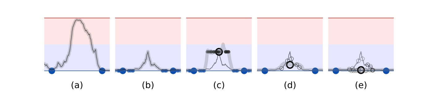
Figure 1: A sketch of a binary classification task with two labeled examples (large blue dots) and one unlabeled example, demonstrating how the choice of the unlabeled target (black circle) affects the fitted function (gray curve). (a) A model with no regularization is free to fit any function that predicts the labeled training examples well. (b) A model trained with noisy labeled data (small dots) learns to give consistent predictions around labeled data points. (c) Consistency to noise around unlabeled examples provides additional smoothing. For the clarity of illustration, the teacher model (gray curve) is first fitted to the labeled examples, and then left unchanged during the training of the student model. Also for clarity, we will omit the small dots in figures d and e. (d) Noise on the teacher model reduces the bias of the targets without additional training. The expected direction of stochastic gradient descent is towards the mean (large blue circle) of individual noisy targets (small blue circles). (e) An ensemble of models gives an even better expected target. Both Temporal Ensembling and the Mean Teacher method use this approach.
图 1:一个二分类任务的示意图,其中有两个有标注样本(大蓝点)和一个无标注样本,用来说明无标注目标(黑圈)的选择如何影响拟合函数(灰线)。(a) 没有正则化的模型可以拟合任何能很好预测有标注训练样本的函数。(b) 用带噪声的有标注数据(小点)训练的模型,会学着在有标注数据点周围给出一致的预测。(c) 对无标注样本周围的噪声保持一致,可以带来额外的平滑。为使图示更清楚,教师模型(灰线)先对有标注样本拟合,并在训练学生模型时保持不变。同样为清楚起见,图 d 和 e 中将省略那些小点。(d) 在教师模型上加噪声,无需额外训练即可减小目标的偏差。随机梯度下降的期望方向指向各个带噪声目标(小蓝圈)的均值(大蓝圈)。(e) 模型的集成能给出更好的期望目标。Temporal Ensembling 和 Mean Teacher 方法都采用了这一思路。
There are at least two ways to improve the target quality. One approach is to choose the perturbation of the representations carefully instead of barely applying additive or multiplicative noise. Another approach is to choose the teacher model carefully instead of barely replicating the student model. Concurrently to our research, Miyato et al. [15] have taken the first approach and shown that Virtual Adversarial Training can yield impressive results. We take the second approach and will show that it too provides significant benefits. To our understanding, these two approaches are compatible, and their combination may produce even better outcomes. However, the analysis of their combined effects is outside the scope of this paper.
至少有两种办法可以提高目标质量。一种是认真选择对表示的扰动,而不是只做简单的加性或乘性噪声。另一种是认真选择教师模型,而不是只复制学生模型。与我们的研究同时,Miyato 等人 [15] 走了第一条路,并表明虚拟对抗训练(Virtual Adversarial Training)可以取得很好的结果。我们走第二条路,并将表明它同样能带来明显收益。在我们看来,这两条路是相容的,结合起来也许会有更好的结果。不过,对二者组合效果的分析超出了本文范围。
Our goal, then, is to form a better teacher model from the student model without additional training. As the first step, consider that the softmax output of a model does not usually provide accurate predictions outside training data. This can be partly alleviated by adding noise to the model at inference time [4], and consequently a noisy teacher can yield more accurate targets (Figure 1d). This approach was used in Pseudo-Ensemble Agreement [2] and has lately been shown to work well on semi-supervised image classification [13, 22]. Laine & Aila [13] named the method the Πmodel; we will use this name for it and their version of it as the basis of our experiments.
于是,我们的目标是:在不做额外训练的前提下,从学生模型构造出一个更好的教师模型。作为第一步,先注意到模型的 softmax 输出在训练数据之外通常并不能给出准确预测。在推理时给模型加噪声,可以部分缓解这一问题 [4],因而一个带噪声的教师可以给出更准确的目标(图 1d)。这一做法曾用于 Pseudo-Ensemble Agreement [2],近来也被表明在半监督图像分类上效果很好 [13, 22]。Laine 和 Aila [13] 把该方法命名为 Πmodel;我们将沿用这一名称,并以他们的版本作为实验的基础。
The Πmodel can be further improved by Temporal Ensembling [13], which maintains an exponential moving average (EMA) prediction for each of the training examples. At each training step, all the EMA predictions of the examples in that minibatch are updated based on the new predictions. Consequently, the EMA prediction of each example is formed by an ensemble of the model's current version and those earlier versions that evaluated the same example. This ensembling improves the quality of the predictions, and using them as the teacher predictions improves results. However, since each target is updated only once per epoch, the learned information is incorporated into the training process at a slow pace. The larger the dataset, the longer the span of the updates, and in the case of on-line learning, it is unclear how Temporal Ensembling can be used at all. (One could evaluate all the targets periodically more than once per epoch, but keeping the evaluation span constant would require evaluations per epoch where is the number of training examples.)
Temporal Ensembling [13] 可以进一步改进 Πmodel:它为每个训练样本维护一个指数滑动平均(EMA)预测。在每个训练步骤,该小批量中所有样本的 EMA 预测都会根据新的预测被更新。于是,每个样本的 EMA 预测,是由模型的当前版本以及曾经评估过同一样本的先前版本共同构成的集成。这种集成提高了预测质量,把它们当作教师预测,结果也会更好。然而,由于每个目标每个 epoch 只更新一次,学到的信息进入训练过程的速度很慢。数据集越大,更新间隔就越长;在在线学习的情形下,甚至不清楚 Temporal Ensembling 该如何使用。(也可以在一个 epoch 内周期性地多次评估全部目标,但若要保持评估间隔不变,每个 epoch 就需要 次评估,其中 是训练样本数。)
2 Mean Teacher
To overcome the limitations of Temporal Ensembling, we propose averaging model weights instead of predictions. Since the teacher model is an average of consecutive student models, we call this the Mean Teacher method (Figure 2). Averaging model weights over training steps tends to produce a more accurate model than using the final weights directly [18]. We can take advantage of this during training to construct better targets. Instead of sharing the weights with the student model, the teacher model uses the EMA weights of the student model. Now it can aggregate information after every step instead of every epoch. In addition, since the weight averages improve all layer outputs, not just the top output, the target model has better intermediate representations. These aspects lead to two practical advantages over Temporal Ensembling: First, the more accurate target labels lead to a faster feedback loop between the student and the teacher models, resulting in better test accuracy. Second, the approach scales to large datasets and on-line learning.
为克服 Temporal Ensembling 的局限,我们建议平均的是模型权重,而不是预测。由于教师模型是连续多个学生模型的平均,我们把这种方法称为 Mean Teacher(图 2)。在训练步骤上对模型权重取平均,往往比直接使用最后得到的权重能得到更准确的模型 [18]。我们可以在训练过程中利用这一点来构造更好的目标。教师模型不再与学生共用同一组权重,而是使用学生权重的 EMA。这样,它就可以在每一步之后聚合信息,而不必等到每个 epoch。此外,权重平均改善的是所有层的输出,而不只是顶层输出,因而目标模型具有更好的中间表示。这些特点相对 Temporal Ensembling 带来两个实际好处:第一,更准确的目标标签使学生和教师之间的反馈环更快,测试准确率也更高;第二,这一方法可以扩展到大型数据集和在线学习。
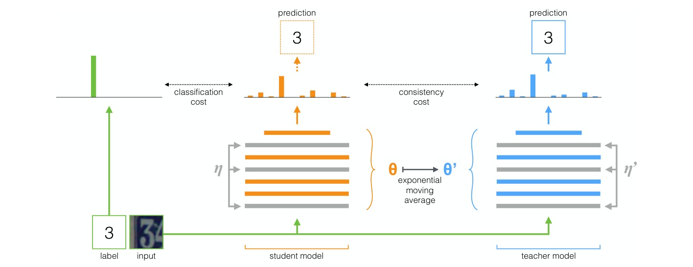
Figure 2: The Mean Teacher method. The figure depicts a training batch with a single labeled example. Both the student and the teacher model evaluate the input applying noise (, ) within their computation. The softmax output of the student model is compared with the one-hot label using classification cost and with the teacher output using consistency cost. After the weights of the student model have been updated with gradient descent, the teacher model weights are updated as an exponential moving average of the student weights. Both model outputs can be used for prediction, but at the end of the training the teacher prediction is more likely to be correct. A training step with an unlabeled example would be similar, except no classification cost would be applied.
图 2:Mean Teacher 方法。图中给出一个只含单个有标注样本的训练批量。学生模型和教师模型都在计算中对输入施加噪声(,)。学生模型的 softmax 输出一方面与 one-hot 标签比较,形成分类代价,另一方面与教师输出比较,形成一致性代价。学生模型的权重用梯度下降更新之后,教师模型的权重再按学生权重的指数滑动平均来更新。两个模型的输出都可以用来预测,但在训练结束时,教师的预测更可能是对的。若训练步骤用的是无标注样本,过程类似,只是不再施加分类代价。
More formally, we define the consistency cost as the expected distance between the prediction of the student model (with weights and noise ) and the prediction of the teacher model (with weights and noise ).
更形式地说,我们把一致性代价 定义为学生模型(权重为 、噪声为 )的预测与教师模型(权重为 、噪声为 )的预测之间的期望距离。
The difference between the Πmodel, Temporal Ensembling, and Mean Teacher is how the teacher predictions are generated. Whereas the Πmodel uses , and Temporal Ensembling approximates with a weighted average of successive predictions, we define at training step as the EMA of successive weights:
Πmodel、Temporal Ensembling 和 Mean Teacher 的差别,在于教师预测是如何生成的。Πmodel 取 ,Temporal Ensembling 用连续多次预测的加权平均来近似 ,而我们把训练步骤 上的 定义为连续多个 权重的 EMA:
where is a smoothing coefficient hyperparameter. An additional difference between the three algorithms is that the Πmodel applies training to whereas Temporal Ensembling and Mean Teacher treat it as a constant with regards to optimization.
其中 是平滑系数超参数。这三种算法还有一个差别:Πmodel 也对 做训练,而 Temporal Ensembling 和 Mean Teacher 在优化时把它视为常数。
We can approximate the consistency cost function by sampling noise , at each training step with stochastic gradient descent. Following Laine & Aila [13], we use mean squared error (MSE) as the consistency cost in most of our experiments.
我们可以在每个训练步骤用随机梯度下降对噪声 、 取样,来近似一致性代价函数 。遵循 Laine 和 Aila [13],我们在大多数实验中用均方误差(MSE)作为一致性代价。
Table 1: Error rate percentage on SVHN over 10 runs (4 runs when using all labels). We use exponential moving average weights in the evaluation of all our models. All the methods use a similar 13-layer ConvNet architecture. See Table 5 in the Appendix for results without input augmentation.
| 250 labels73257 images | 500 labels73257 images | 1000 labels73257 images | 73257 labels73257 images | |
|---|---|---|---|---|
| GAN [24] | ||||
| Πmodel [13] | ||||
| Temporal Ensembling [13] | ||||
| VAT+EntMin [15] | 3.86 | |||
| Supervised-only | ||||
| Πmodel | ||||
| Mean Teacher |
表 1:SVHN 上的错误率(百分比),共 10 次运行(使用全部标签时为 4 次)。评估我们的全部模型时,都使用指数滑动平均权重。所有方法都使用相近的 13 层 ConvNet 结构。不使用输入增广的结果见附录中的表 5。
| 250 个标签73257 张图像 | 500 个标签73257 张图像 | 1000 个标签73257 张图像 | 73257 个标签73257 张图像 | |
|---|---|---|---|---|
| GAN [24] | ||||
| Πmodel [13] | ||||
| Temporal Ensembling [13] | ||||
| VAT+EntMin [15] | 3.86 | |||
| Supervised-only | ||||
| Πmodel | ||||
| Mean Teacher |
Table 2: Error rate percentage on CIFAR-10 over 10 runs (4 runs when using all labels).
| 1000 labels50000 images | 2000 labels50000 images | 4000 labels50000 images | 50000 labels50000 images | |
|---|---|---|---|---|
| GAN [24] | ||||
| Πmodel [13] | ||||
| Temporal Ensembling [13] | ||||
| VAT+EntMin [15] | 10.55 | |||
| Supervised-only | ||||
| Πmodel | ||||
| Mean Teacher |
表 2:CIFAR-10 上的错误率(百分比),共 10 次运行(使用全部标签时为 4 次)。
| 1000 个标签50000 张图像 | 2000 个标签50000 张图像 | 4000 个标签50000 张图像 | 50000 个标签50000 张图像 | |
|---|---|---|---|---|
| GAN [24] | ||||
| Πmodel [13] | ||||
| Temporal Ensembling [13] | ||||
| VAT+EntMin [15] | 10.55 | |||
| Supervised-only | ||||
| Πmodel | ||||
| Mean Teacher |
3 Experiments
3 实验
To test our hypotheses, we first replicated the Πmodel [13] in TensorFlow [1] as our baseline. We then modified the baseline model to use weight-averaged consistency targets. The model architecture is a 13-layer convolutional neural network (ConvNet) with three types of noise: random translations and horizontal flips of the input images, Gaussian noise on the input layer, and dropout applied within the network. We use mean squared error as the consistency cost and ramp up its weight from 0 to its final value during the first 80 epochs. The details of the model and the training procedure are described in Appendix B.1.
为检验我们的假设,我们首先在 TensorFlow [1] 中复现了 Πmodel [13],作为基线。随后我们修改基线模型,改用权重平均的一致性目标。模型结构是一个 13 层卷积神经网络(ConvNet),并使用三类噪声:输入图像的随机平移和水平翻转、输入层上的高斯噪声,以及网络内部的 dropout。一致性代价使用均方误差,并在前 80 个 epoch 里把它的权重从 0 逐步升到最终值。模型和训练过程的细节见附录 B.1。
3.1 Comparison to other methods on SVHN and CIFAR-10
3.1 在 SVHN 和 CIFAR-10 上与其他方法的比较
We ran experiments using the Street View House Numbers (SVHN) and CIFAR-10 benchmarks [16]. Both datasets contain 32x32 pixel RGB images belonging to ten different classes. In SVHN, each example is a close-up of a house number, and the class represents the identity of the digit at the center of the image. In CIFAR-10, each example is a natural image belonging to a class such as horses, cats, cars and airplanes. SVHN contains of 73257 training samples and 26032 test samples. CIFAR-10 consists of 50000 training samples and 10000 test samples.
我们在 Street View House Numbers(SVHN)和 CIFAR-10 基准 [16] 上做了实验。这两个数据集都包含属于十个不同类别的 像素 RGB 图像。在 SVHN 中,每个样本是门牌号的近景,类别表示图像中心那个数字的身份。在 CIFAR-10 中,每个样本是一幅自然图像,类别包括马、猫、汽车和飞机等。SVHN 包含 73257 个训练样本和 26032 个测试样本。CIFAR-10 包含 50000 个训练样本和 10000 个测试样本。
Tables 1 and 2 compare the results against recent state-of-the-art methods. All the methods in the comparison use a similar 13-layer ConvNet architecture. Mean Teacher improves test accuracy over the Πmodel and Temporal Ensembling on semi-supervised SVHN tasks. Mean Teacher also improves results on CIFAR-10 over our baseline Πmodel.
表 1 和表 2 把结果与近期最好的方法做了比较。比较中的所有方法都使用相近的 13 层 ConvNet 结构。在半监督的 SVHN 任务上,Mean Teacher 的测试准确率高于 Πmodel 和 Temporal Ensembling。在 CIFAR-10 上,Mean Teacher 也优于我们的 Πmodel 基线。
The recently published version of Virtual Adversarial Training by Miyato et al. [15] performs even better than Mean Teacher on the 1000-label SVHN and the 4000-label CIFAR-10. As discussed in the introduction, VAT and Mean Teacher are complimentary approaches. Their combination may yield better accuracy than either of them alone, but that investigation is beyond the scope of this paper.
Miyato 等人 [15] 最近发表的虚拟对抗训练版本,在 1000 个标签的 SVHN 和 4000 个标签的 CIFAR-10 上比 Mean Teacher 还要好。如引言所述,VAT 和 Mean Teacher 是互补的方法。二者结合也许会比单独使用其中任何一种得到更高的准确率,但这一考察超出了本文范围。
Table 3: Error percentage over 10 runs on SVHN with extra unlabeled training data.
| 500 labels73257 images | 500 labels173257 images | 500 labels573257 images | |
|---|---|---|---|
| Πmodel (ours) | |||
| Mean Teacher |
表 3:在 SVHN 上使用额外无标注训练数据时的错误率(百分比),共 10 次运行。
| 500 个标签73257 张图像 | 500 个标签173257 张图像 | 500 个标签573257 张图像 | |
|---|---|---|---|
| Πmodel (ours) | |||
| Mean Teacher |
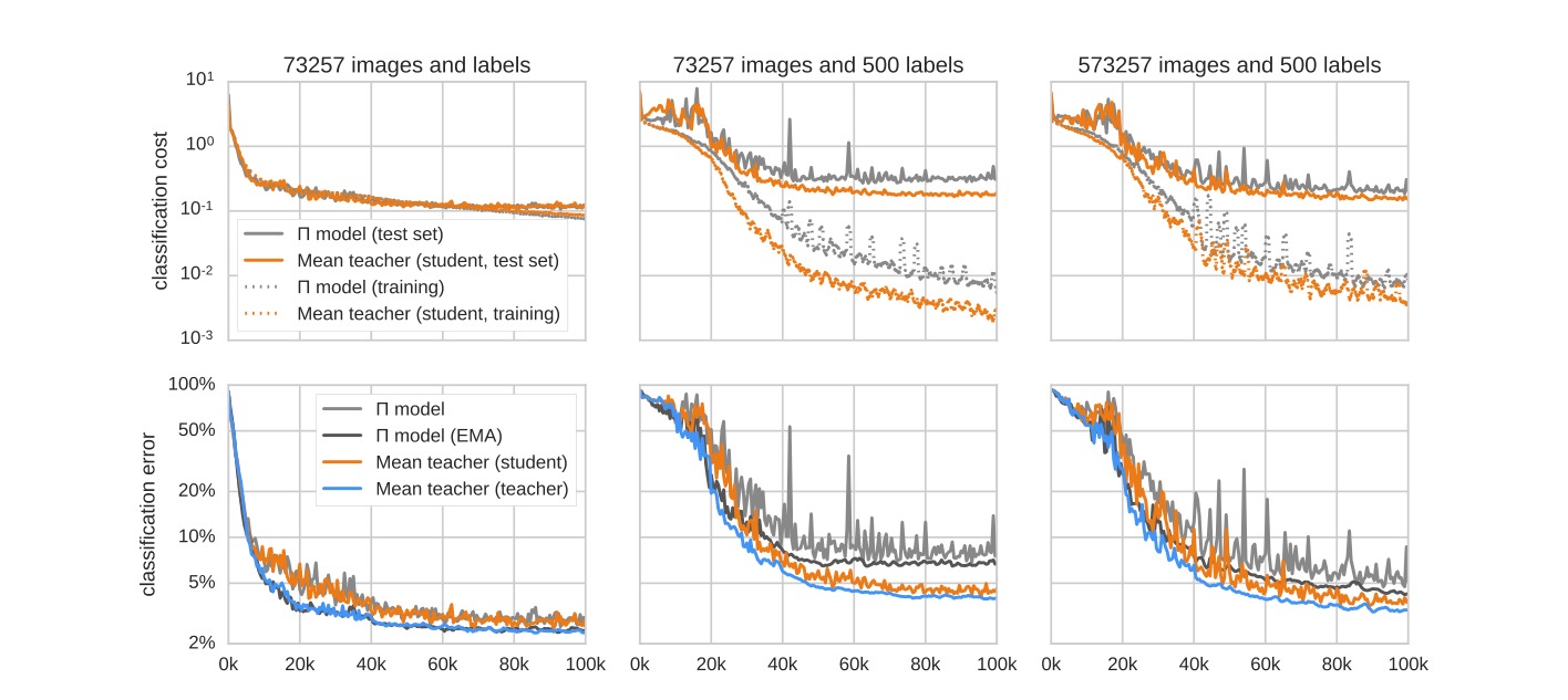
Figure 3: Smoothened classification cost (top) and classification error (bottom) of Mean Teacher and our baseline Πmodel on SVHN over the first 100000 training steps. In the upper row, the training classification costs are measured using only labeled data.
图 3:Mean Teacher 与我们的基线 Πmodel 在 SVHN 上前 100000 个训练步骤的平滑分类代价(上)和分类错误率(下)。上行中,训练分类代价只在有标注数据上测量。
3.2 SVHN with extra unlabeled data
3.2 使用额外无标注数据的 SVHN
Above, we suggested that Mean Teacher scales well to large datasets and on-line learning. In addition, the SVHN and CIFAR-10 results indicate that it uses unlabeled examples efficiently. Therefore, we wanted to test whether we have reached the limits of our approach.
上文我们提出,Mean Teacher 能够很好地扩展到大型数据集和在线学习。此外,SVHN 和 CIFAR-10 上的结果也表明,它能高效地利用无标注样本。因此,我们想检验是否已经触及这种方法的上限。
Besides the primary training data, SVHN includes also an extra dataset of 531131 examples. We picked 500 samples from the primary training as our labeled training examples. We used the rest of the primary training set together with the extra training set as unlabeled examples. We ran experiments with Mean Teacher and our baseline Πmodel, and used either 0, 100000 or 500000 extra examples. Table 3 shows the results.
除了主要训练数据外,SVHN 还包含一个有 531131 个样本的额外数据集。我们从主要训练集中取出 500 个样本作为有标注的训练样本,并把主要训练集的其余部分与额外训练集一起作为无标注样本。我们用 Mean Teacher 和基线 Πmodel 做了实验,额外样本数分别取 0、100000 或 500000。结果见表 3。
3.3 Analysis of the training curves
3.3 对训练曲线的分析
The training curves on Figure 3 help us understand the effects of using Mean Teacher. As expected, the EMA-weighted models (blue and dark gray curves in the bottom row) give more accurate predictions than the bare student models (orange and light gray) after an initial period.
图 3 中的训练曲线帮助我们理解使用 Mean Teacher 的效果。如所预期,经过一段初始阶段之后,EMA 加权的模型(下行中的蓝色和深灰色曲线)比单纯的学生模型(橙色和浅灰色)给出更准确的预测。
Using the EMA-weighted model as the teacher improves results in the semi-supervised settings. There appears to be a virtuous feedback cycle of the teacher (blue curve) improving the student (orange) via the consistency cost, and the student improving the teacher via exponential moving averaging. If this feedback cycle is detached, the learning is slower, and the model starts to overfit earlier (dark gray and light gray).
在半监督设定中,用 EMA 加权的模型作为教师可以改进结果。这里似乎存在一个良性反馈循环:教师(蓝色曲线)通过一致性代价改进学生(橙色),学生再通过指数滑动平均改进教师。如果切断这一反馈循环,学习会变慢,模型也会更早开始过拟合(深灰色和浅灰色)。
Mean Teacher helps when labels are scarce. When using 500 labels (middle column) Mean Teacher learns faster, and continues training after the Πmodel stops improving. On the other hand, in the all-labeled case (left column), Mean Teacher and the Πmodel behave virtually identically.
在标签稀少时,Mean Teacher 更有帮助。使用 500 个标签时(中列),Mean Teacher 学得更快,并且在 Πmodel 不再提升之后仍继续训练。另一方面,在全部有标注的情形下(左列),Mean Teacher 与 Πmodel 的表现几乎相同。
Mean Teacher uses unlabeled training data more efficiently than the Πmodel, as seen in the middle column. On the other hand, with 500k extra unlabeled examples (right column), Πmodel keeps improving for longer. Mean Teacher learns faster, and eventually converges to a better result, but the sheer amount of data appears to offset Πmodel's worse predictions.
如中列所示,Mean Teacher 比 Πmodel 更有效地使用无标注训练数据。另一方面,在有 50 万额外无标注样本时(右列),Πmodel 会在更长时间里持续改进。Mean Teacher 学得更快,最终也收敛到更好的结果,但海量数据似乎弥补了 Πmodel 较差的预测。
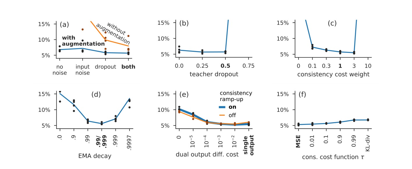
Figure 4: Validation error on 250-label SVHN over four runs per hyperparameter setting and their means. In each experiment, we varied one hyperparameter, and used the evaluation run hyperparameters of Table 1 for the rest. The hyperparameter settings used in the evaluation runs are marked with the bolded font weight. See the text for details.
图 4:在 250 个标签的 SVHN 上,每种超参数设置四次运行的验证错误率及其均值。每次实验只改变一个超参数,其余使用表 1 中评估运行的超参数。评估运行所用的超参数设置以粗体标出。细节见正文。
3.4 Ablation experiments
3.4 消融实验
To assess the importance of various aspects of the model, we ran experiments on SVHN with 250 labels, varying one or a few hyperparameters at a time while keeping the others fixed.
为评估模型各个方面的重要性,我们在只有 250 个标签的 SVHN 上做了实验,每次改变一个或几个超参数,其余保持固定。
Removal of noise (Figures 4(a) and 4(b)). In the introduction and Figure 1, we presented the hypothesis that the Πmodel produces better predictions by adding noise to the model on both sides. But after the addition of Mean Teacher, is noise still needed? Yes. We can see that either input augmentation or dropout is necessary for passable performance. On the other hand, input noise does not help when augmentation is in use. Dropout on the teacher side provides only a marginal benefit over just having it on the student side, at least when input augmentation is in use.
去掉噪声(图 4(a) 和 4(b))。在引言和图 1 中,我们提出这样的假设:Πmodel 通过在师生两侧都给模型加噪声来得到更好的预测。但在加入 Mean Teacher 之后,还需要噪声吗?需要。可以看到,要达到尚可的性能,输入增广或 dropout 至少得有一种。另一方面,在已经使用增广时,输入噪声并无帮助。至少在使用输入增广时,只在教师一侧再加 dropout,相对只在学生一侧使用,带来的好处很有限。
Sensitivity to EMA decay and consistency weight (Figures 4(c) and 4(d)). The essential hyperparameters of the Mean Teacher algorithm are the consistency cost weight and the EMA decay . How sensitive is the algorithm to their values? We can see that in each case the good values span roughly an order of magnitude and outside these ranges the performance degrades quickly. Note that EMA decay makes the model a variation of the Πmodel, although somewhat inefficient one because the gradients are propagated through only the student path. Note also that in the evaluation runs we used EMA decay during the ramp-up phase, and for the rest of the training. We chose this strategy because the student improves quickly early in the training, and thus the teacher should forget the old, inaccurate, student weights quickly. Later the student improvement slows, and the teacher benefits from a longer memory.
对 EMA 衰减和一致性权重的敏感性(图 4(c) 和 4(d))。Mean Teacher 算法的关键超参数是一致性代价的权重以及 EMA 衰减 。算法对它们的取值有多敏感?可以看到,在这两种情形下,较好的取值大约各跨越一个数量级,超出这些范围后性能会迅速下降。注意,EMA 衰减 会使模型变成 Πmodel 的一个变体,只不过效率稍差,因为梯度只沿学生路径回传。还要注意,在评估运行中,我们在升温阶段使用 EMA 衰减 ,其余训练使用 。选择这一策略是因为学生在训练初期提升很快,教师应当迅速忘掉旧的、不够准确的学生权重;随后学生的提升变慢,教师就能从更长的记忆中获益。
Decoupling classification and consistency (Figure 4(e)). The consistency to teacher predictions may not necessarily be a good proxy for the classification task, especially early in the training. So far our model has strongly coupled these two tasks by using the same output for both. How would decoupling the tasks change the performance of the algorithm? To investigate, we changed the model to have two top layers and produce two outputs. We then trained one of the outputs for classification and the other for consistency. We also added a mean squared error cost between the output logits, and then varied the weight of this cost, allowing us to control the strength of the coupling. Looking at the results (reported using the EMA version of the classification output), we can see that the strongly coupled version performs well and the too loosely coupled versions do not. On the other hand, a moderate decoupling seems to have the benefit of making the consistency ramp-up redundant.
把分类与一致性解耦(图 4(e))。与教师预测保持一致,未必是分类任务的良好代理,尤其是在训练早期。到目前为止,我们的模型用同一个输出同时承担这两项任务,从而把它们紧紧耦合在一起。如果把任务解耦,算法的性能会怎样变化?为考察这一点,我们把模型改成有两个顶层、产生两个输出,然后用其中一个输出训练分类,用另一个训练一致性。我们还在输出 logits 之间加了一项均方误差代价,并改变这项代价的权重,以控制耦合的强度。从结果(按分类输出的 EMA 版本报告)可以看到,强耦合的版本表现很好,耦合过松的版本则不然。另一方面,适度解耦似乎还有一个好处,就是不再需要一致性代价的升温。
Table 4: Error rate percentage of ResNet Mean Teacher compared to the state of the art. We report the test results from 10 runs on CIFAR-10 and validation results from 2 runs on ImageNet.
| CIFAR-104000 labels | ImageNet 201210% of the labels | |
|---|---|---|
| State of the art | 10.55 [15] | [19] |
| ConvNet Mean Teacher | ||
| ResNet Mean Teacher | ||
| State of the art using all labels | 2.86 [5] | 3.79 [10] |
表 4:ResNet Mean Teacher 的错误率(百分比)与当时最好结果的比较。CIFAR-10 报告 10 次运行的测试结果,ImageNet 报告 2 次运行的验证结果。
| CIFAR-104000 个标签 | ImageNet 201210% 的标签 | |
|---|---|---|
| State of the art | 10.55 [15] | [19] |
| ConvNet Mean Teacher | ||
| ResNet Mean Teacher | ||
| State of the art using all labels | 2.86 [5] | 3.79 [10] |
Changing from MSE to KL-divergence (Figure 4(f)). Following Laine & Aila [13], we use mean squared error (MSE) as our consistency cost function, but KL-divergence would seem a more natural choice. Which one works better? We ran experiments with instances of a cost function family ranging from MSE ( in the figure) to KL-divergence (), and found out that in this setting MSE performs better than the other cost functions. See Appendix C for the details of the cost function family and for our intuition about why MSE performs so well.
从 MSE 改到 KL 散度(图 4(f))。遵循 Laine 和 Aila [13],我们用均方误差(MSE)作为一致性代价函数,但 KL 散度看起来是更自然的选择。哪一种更好?我们在一个从 MSE(图中 )到 KL 散度()的代价函数族上做了实验,发现在这一设定下,MSE 比其他代价函数表现更好。关于这一代价函数族的细节,以及我们对 MSE 为何表现如此之好的直觉,见附录 C。
3.5 Mean Teacher with residual networks on CIFAR-10 and ImageNet
3.5 在 CIFAR-10 和 ImageNet 上使用残差网络的 Mean Teacher
In the experiments above, we used a traditional 13-layer convolutional architecture (ConvNet), which has the benefit of making comparisons to earlier work easy. In order to explore the effect of the model architecture, we ran experiments using a 12-block (26-layer) Residual Network [8] (ResNet) with Shake-Shake regularization [5] on CIFAR-10. The details of the model and the training procedure are described in Appendix B.2. As shown in Table 4, the results improve remarkably with the better network architecture.
在上面的实验中,我们使用了传统的 13 层卷积结构(ConvNet),好处是便于与先前工作比较。为考察模型结构的影响,我们在 CIFAR-10 上用带 Shake-Shake 正则化 [5] 的 12 个块(26 层)残差网络 [8](ResNet)做了实验。模型和训练过程的细节见附录 B.2。如表 4 所示,更好的网络结构使结果有了显著提升。
To test whether the methods scales to more natural images, we ran experiments on Imagenet 2012 dataset [21] using 10% of the labels. We used a 50-block (152-layer) ResNeXt architecture [32], and saw a clear improvement over the state of the art. As the test set is not publicly available, we measured the results using the validation set.
为检验这些方法能否扩展到更自然的图像,我们在 ImageNet 2012 数据集 [21] 上使用 10% 的标签做了实验。我们使用 50 个块(152 层)的 ResNeXt 结构 [32],看到对当时最好结果有明显改进。由于测试集不公开,我们用验证集来衡量结果。
4 Related work
4 相关工作
Noise regularization of neural networks was proposed by Sietsma & Dow [25]. More recently, several types of perturbations have been shown to regularize intermediate representations effectively in deep learning. Adversarial Training [6] changes the input slightly to give predictions that are as different as possible from the original predictions. Dropout [27] zeroes random dimensions of layer outputs. Dropconnect [30] generalizes Dropout by zeroing individual weights instead of activations. Stochastic Depth [11] drops entire layers of residual networks, and Swapout [26] generalizes Dropout and Stochastic Depth. Shake-shake regularization [5] duplicates residual paths and samples a linear combination of their outputs independently during forward and backward passes.
神经网络的噪声正则化由 Sietsma 和 Dow [25] 提出。更近一些,已有若干类型的扰动被表明能有效正则化深度学习中的中间表示。对抗训练 [6] 对输入做轻微改动,使预测与原来的预测尽可能不同。Dropout [27] 将层输出的随机若干维置零。Dropconnect [30] 把 Dropout 推广为对单个权重而不是激活值置零。Stochastic Depth [11] 丢掉残差网络的整层,Swapout [26] 则推广了 Dropout 和 Stochastic Depth。Shake-shake 正则化 [5] 复制残差路径,并在前向和反向传播中分别对它们输出的线性组合取样。
Several semi-supervised methods are based on training the model predictions to be consistent to perturbation. The Denoising Source Separation framework (DSS) [28] uses denoising of latent variables to learn their likelihood estimate. The Γ variant of Ladder Network [20] implements DSS with a deep learning model for classification tasks. It produces a noisy student predictions and clean teacher predictions, and applies a denoising layer to predict teacher predictions from the student predictions. The Πmodel [13] improves the Γ model by removing the explicit denoising layer and applying noise also to the teacher predictions. Similar methods had been proposed already earlier for linear models [29] and deep learning [2]. Virtual Adversarial Training [15] is similar to the Πmodel but uses adversarial perturbation instead of independent noise.
有若干半监督方法的基础,是训练模型预测使之对扰动保持一致。Denoising Source Separation 框架(DSS)[28] 通过对潜变量去噪来学习它们的似然估计。Ladder Network 的 Γ 变体 [20] 用深度学习模型在分类任务上实现了 DSS。它产生带噪声的学生预测和干净的教师预测,并使用一个去噪层,从学生预测去预测教师预测。Πmodel [13] 改进了 Γ 模型:去掉显式的去噪层,并对教师预测也施加噪声。类似的方法更早已针对线性模型 [29] 和深度学习 [2] 提出。虚拟对抗训练 [15] 与 Πmodel 类似,但使用的是对抗扰动,而不是独立噪声。
The idea of a teacher model training a student is related to model compression [3] and distillation [9]. The knowledge of a complicated model can be transferred to a simpler model by training the simpler model with the softmax outputs of the complicated model. The softmax outputs contain more information about the task than the one-hot outputs, and the requirement of representing this knowledge regularizes the simpler model. Besides its use in model compression, distillation can be used to harden trained models against adversarial attacks [17]. The difference between distillation and consistency regularization is that distillation is performed after training whereas consistency regularization is performed on training time.
用教师模型训练学生,这一想法与模型压缩 [3] 和蒸馏 [9] 有关。把复杂模型的知识迁到更简单的模型,可以通过用复杂模型的 softmax 输出去训练简单模型来完成。softmax 输出比 one-hot 输出包含更多关于任务的信息,而表示这些知识的要求会对简单模型形成正则。除了用于模型压缩,蒸馏还可以用来增强已训练模型对对抗攻击的抵抗力 [17]。蒸馏与一致性正则化的差别在于:蒸馏是在训练之后进行的,而一致性正则化是在训练过程中进行的。
Consistency regularization can be seen as a form of label propagation [33]. Training samples that resemble each other are more likely to belong to the same class. Label propagation takes advantage of this assumption by pushing label information from each example to examples that are near it according to some metric. Label propagation can also be applied to deep learning models [31]. However, ordinary label propagation requires a predefined distance metric in the input space. In contrast, consistency targets employ a learned distance metric implied by the abstract representations of the model. As the model learns new features, the distance metric changes to accommodate these features. Therefore, consistency targets guide learning in two ways. On the one hand they spread the labels according to the current distance metric, and on the other hand, they aid the network learn a better distance metric.
一致性正则化也可以看成一种标签传播 [33]。彼此相似的训练样本更可能属于同一类。标签传播利用这一假定,按某种度量把标签信息从每个样本推到邻近的样本。标签传播也可以用于深度学习模型 [31]。不过,普通的标签传播需要在输入空间中预先定义距离度量。相比之下,一致性目标使用的是由模型抽象表示所隐含的、学到的距离度量。随着模型学到新的特征,这一距离度量也会随之调整。因此,一致性目标从两个方面引导学习:一方面按当前的距离度量传播标签,另一方面帮助网络学到更好的距离度量。
5 Conclusion
5 结论
Temporal Ensembling, Virtual Adversarial Training and other forms of consistency regularization have recently shown their strength in semi-supervised learning. In this paper, we propose Mean Teacher, a method that averages model weights to form a target-generating teacher model. Unlike Temporal Ensembling, Mean Teacher works with large datasets and on-line learning. Our experiments suggest that it improves the speed of learning and the classification accuracy of the trained network. In addition, it scales well to state-of-the-art architectures and large image sizes.
Temporal Ensembling、虚拟对抗训练以及其他形式的一致性正则化,近来已在半监督学习中显示出实力。本文提出 Mean Teacher,通过平均模型权重来构成一个生成目标的教师模型。与 Temporal Ensembling 不同,Mean Teacher 可用于大型数据集和在线学习。我们的实验表明,它能提高学习速度以及所训练网络的分类准确率。此外,它也能很好地扩展到当时最好的网络结构和更大的图像尺寸。
The success of consistency regularization depends on the quality of teacher-generated targets. If the targets can be improved, they should be. Mean Teacher and Virtual Adversarial Training represent two ways of exploiting this principle. Their combination may yield even better targets. There are probably additional methods to be uncovered that improve targets and trained models even further.
一致性正则化能否成功,取决于教师生成的目标质量。如果目标还能改进,就应当改进。Mean Teacher 和虚拟对抗训练代表了利用这一原则的两条路。二者结合也许能得到更好的目标。很可能还有更多有待发现的方法,能进一步改进目标和训练得到的模型。
Acknowledgements
致谢
We thank Samuli Laine and Timo Aila for fruitful discussions about their work, and Phil Bachman and Colin Raffel for corrections to the pre-print version of this paper. We also thank everyone at The Curious AI Company for their help, encouragement, and ideas.
我们感谢 Samuli Laine 和 Timo Aila 就他们的工作与我们进行了富有成果的讨论,感谢 Phil Bachman 和 Colin Raffel 对本文预印本提出的修正。我们也感谢 The Curious AI Company 的每一位同事给予的帮助、鼓励和想法。
References
参考文献
[1] Abadi, Martín, Agarwal, Ashish, Barham, Paul, Brevdo, Eugene, Chen, Zhifeng, Citro, Craig, Corrado, Greg S., Davis, Andy, Dean, Jeffrey, Devin, Matthieu, Ghemawat, Sanjay, Goodfellow, Ian, Harp, Andrew, Irving, Geoffrey, Isard, Michael, Jia, Yangqing, Jozefowicz, Rafal, Kaiser, Lukasz, Kudlur, Manjunath, Levenberg, Josh, Mané, Dan, Monga, Rajat, Moore, Sherry, Murray, Derek, Olah, Chris, Schuster, Mike, Shlens, Jonathon, Steiner, Benoit, Sutskever, Ilya, Talwar, Kunal, Tucker, Paul, Vanhoucke, Vincent, Vasudevan, Vijay, Viégas, Fernanda, Vinyals, Oriol, Warden, Pete, Wattenberg, Martin, Wicke, Martin, Yu, Yuan, and Zheng, Xiaoqiang. TensorFlow: Large-Scale Machine Learning on Heterogeneous Systems. 2015.
[2] Bachman, Philip, Alsharif, Ouais, and Precup, Doina. Learning with Pseudo-Ensembles. arXiv:1412.4864 [cs, stat], December 2014. arXiv: 1412.4864.
[3] Buciluˇa, Cristian, Caruana, Rich, and Niculescu-Mizil, Alexandru. Model compression. In Proceedings of the 12th ACM SIGKDD international conference on Knowledge discovery and data mining, pp. 535–541. ACM, 2006.
[4] Gal, Yarin and Ghahramani, Zoubin. Dropout as a Bayesian Approximation: Representing Model Uncertainty in Deep Learning. In Proceedings of The 33rd International Conference on Machine Learning, pp. 1050–1059, 2016.
[5] Gastaldi, Xavier. Shake-Shake regularization. arXiv:1705.07485 [cs], May 2017. arXiv: 1705.07485.
[6] Goodfellow, Ian J., Shlens, Jonathon, and Szegedy, Christian. Explaining and Harnessing Adversarial Examples. December 2014. arXiv: 1412.6572.
[7] Guo, Chuan, Pleiss, Geoff, Sun, Yu, and Weinberger, Kilian Q. On Calibration of Modern Neural Networks. arXiv:1706.04599 [cs], June 2017. arXiv: 1706.04599.
[8] He, Kaiming, Zhang, Xiangyu, Ren, Shaoqing, and Sun, Jian. Deep Residual Learning for Image Recognition. arXiv:1512.03385 [cs], December 2015. arXiv: 1512.03385.
[9] Hinton, Geoffrey, Vinyals, Oriol, and Dean, Jeff. Distilling the Knowledge in a Neural Network. arXiv:1503.02531 [cs, stat], March 2015. arXiv: 1503.02531.
[10] Hu, Jie, Shen, Li, and Sun, Gang. Squeeze-and-Excitation Networks. arXiv:1709.01507 [cs], September 2017. arXiv: 1709.01507.
[11] Huang, Gao, Sun, Yu, Liu, Zhuang, Sedra, Daniel, and Weinberger, Kilian. Deep Networks with Stochastic Depth. arXiv:1603.09382 [cs], March 2016. arXiv: 1603.09382.
[12] Kingma, Diederik and Ba, Jimmy. Adam: A Method for Stochastic Optimization. arXiv:1412.6980 [cs], December 2014. arXiv: 1412.6980.
[13] Laine, Samuli and Aila, Timo. Temporal Ensembling for Semi-Supervised Learning. arXiv:1610.02242 [cs], October 2016. arXiv: 1610.02242.
[14] Maas, Andrew L., Hannun, Awni Y., and Ng, Andrew Y. Rectifier nonlinearities improve neural network acoustic models. In Proc. ICML, volume 30, 2013.
[15] Miyato, Takeru, Maeda, Shin-ichi, Koyama, Masanori, and Ishii, Shin. Virtual Adversarial Training: a Regularization Method for Supervised and Semi-supervised Learning. arXiv:1704.03976 [cs, stat], April 2017. arXiv: 1704.03976.
[16] Netzer, Yuval, Wang, Tao, Coates, Adam, Bissacco, Alessandro, Wu, Bo, and Ng, Andrew Y. Reading digits in natural images with unsupervised feature learning. In NIPS Workshop on Deep Learning and Unsupervised Feature Learning, 2011.
[17] Papernot, Nicolas, McDaniel, Patrick, Wu, Xi, Jha, Somesh, and Swami, Ananthram. Distillation as a Defense to Adversarial Perturbations against Deep Neural Networks. arXiv:1511.04508 [cs, stat], November 2015. arXiv: 1511.04508.
[18] Polyak, B. T. and Juditsky, A. B. Acceleration of Stochastic Approximation by Averaging. SIAM J. Control Optim., 30(4):838–855, July 1992. ISSN 0363-0129. doi: 10.1137/0330046.
[19] Pu, Yunchen, Gan, Zhe, Henao, Ricardo, Yuan, Xin, Li, Chunyuan, Stevens, Andrew, and Carin, Lawrence. Variational Autoencoder for Deep Learning of Images, Labels and Captions. arXiv:1609.08976 [cs, stat], September 2016. arXiv: 1609.08976.
[20] Rasmus, Antti, Berglund, Mathias, Honkala, Mikko, Valpola, Harri, and Raiko, Tapani. Semi-supervised Learning with Ladder Networks. In Cortes, C., Lawrence, N. D., Lee, D. D., Sugiyama, M., and Garnett, R. (eds.), Advances in Neural Information Processing Systems 28, pp. 3546–3554. Curran Associates, Inc., 2015.
[21] Russakovsky, Olga, Deng, Jia, Su, Hao, Krause, Jonathan, Satheesh, Sanjeev, Ma, Sean, Huang, Zhiheng, Karpathy, Andrej, Khosla, Aditya, Bernstein, Michael, Berg, Alexander C., and Fei-Fei, Li. ImageNet Large Scale Visual Recognition Challenge. arXiv:1409.0575 [cs], September 2014. arXiv: 1409.0575.
[22] Sajjadi, Mehdi, Javanmardi, Mehran, and Tasdizen, Tolga. Regularization With Stochastic Transformations and Perturbations for Deep Semi-Supervised Learning. In Lee, D. D., Sugiyama, M., Luxburg, U. V., Guyon, I., and Garnett, R. (eds.), Advances in Neural Information Processing Systems 29, pp. 1163–1171. Curran Associates, Inc., 2016.
[23] Salimans, Tim and Kingma, Diederik P. Weight normalization: A simple reparameterization to accelerate training of deep neural networks. In Advances in Neural Information Processing Systems, pp. 901–901, 2016.
[24] Salimans, Tim, Goodfellow, Ian, Zaremba, Wojciech, Cheung, Vicki, Radford, Alec, and Chen, Xi. Improved techniques for training gans. In Advances in Neural Information Processing Systems, pp. 2226–2234, 2016.
[25] Sietsma, Jocelyn and Dow, Robert JF. Creating artificial neural networks that generalize. Neural networks, 4(1):67–79, 1991.
[26] Singh, Saurabh, Hoiem, Derek, and Forsyth, David. Swapout: Learning an ensemble of deep architectures. arXiv:1605.06465 [cs], May 2016. arXiv: 1605.06465.
[27] Srivastava, Nitish, Hinton, Geoffrey, Krizhevsky, Alex, Sutskever, Ilya, and Salakhutdinov, Ruslan. Dropout: A Simple Way to Prevent Neural Networks from Overfitting. J. Mach. Learn. Res., 15(1):1929–1958, January 2014. ISSN 1532-4435.
[28] Särelä, Jaakko and Valpola, Harri. Denoising Source Separation. Journal of Machine Learning Research, 6(Mar):233–272, 2005. ISSN ISSN 1533-7928.
[29] Wager, Stefan, Wang, Sida, and Liang, Percy. Dropout Training as Adaptive Regularization. arXiv:1307.1493 [cs, stat], July 2013. arXiv: 1307.1493.
[30] Wan, Li, Zeiler, Matthew, Zhang, Sixin, Le Cun, Yann, and Fergus, Rob. Regularization of Neural Networks using DropConnect. pp. 1058–1066, 2013.
[31] Weston, Jason, Ratle, Frédéric, Mobahi, Hossein, and Collobert, Ronan. Deep learning via semi-supervised embedding. In Neural Networks: Tricks of the Trade, pp. 639–655. Springer, 2012.
[32] Xie, Saining, Girshick, Ross, Dollár, Piotr, Tu, Zhuowen, and He, Kaiming. Aggregated Residual Transformations for Deep Neural Networks. arXiv:1611.05431 [cs], November 2016. arXiv: 1611.05431.
[33] Zhu, Xiaojin and Ghahramani, Zoubin. Learning from labeled and unlabeled data with label propagation. 2002.