Towards Deep Learning Models Resistant to Adversarial Attacks
Towards Deep Learning Models Resistant to Adversarial Attacks
迈向抗对抗攻击的深度学习模型
Aleksander Mądry Thanks: Authors ordered alphabetically. Affiliation: MIT Email: madry@mit.edu Aleksandar Makelov 1 1 footnotemark: 1 Affiliation: MIT Email: amakelov@mit.edu Ludwig Schmidt 1 1 footnotemark: 1 Affiliation: MIT Email: ludwigs@mit.edu Dimitris Tsipras 1 1 footnotemark: 1 Affiliation: MIT Email: tsipras@mit.edu Adrian Vladu 1 1 footnotemark: 1 Affiliation: MIT Email: avladu@mit.edu
Abstract
摘要
Recent work has demonstrated that deep neural networks are vulnerable to adversarial examples—inputs that are almost indistinguishable from natural data and yet classified incorrectly by the network. In fact, some of the latest findings suggest that the existence of adversarial attacks may be an inherent weakness of deep learning models. To address this problem, we study the adversarial robustness of neural networks through the lens of robust optimization. This approach provides us with a broad and unifying view on much of the prior work on this topic. Its principled nature also enables us to identify methods for both training and attacking neural networks that are reliable and, in a certain sense, universal. In particular, they specify a concrete security guarantee that would protect against any adversary. These methods let us train networks with significantly improved resistance to a wide range of adversarial attacks. They also suggest the notion of security against a first-order adversary as a natural and broad security guarantee. We believe that robustness against such well-defined classes of adversaries is an important stepping stone towards fully resistant deep learning models. [^1]
近期工作表明,深度神经网络易受对抗样本攻击——这些输入与自然数据几乎无法区分,却会被网络错误分类。事实上,部分最新发现暗示对抗攻击的存在或许是深度学习模型的固有弱点。为应对这一问题,我们从鲁棒优化的视角研究神经网络的对抗鲁棒性。该视角为我们审视该主题上大量先前工作提供了宽广且统一的框架。其原则性也使我们能识别出既可靠、在某种意义上又具普适性的训练与攻击神经网络的方法。具体而言,它们给出可抵御任意对手的具体安全保证。这些方法使我们能训练出对广泛对抗攻击抵抗力显著增强的网络,并提示「对一阶对手的安全性」可作为自然且宽广的安全保证。我们认为,针对此类定义清晰的对手类别的鲁棒性,是迈向完全抗攻击深度学习模型的重要踏脚石。[^1]
1 Introduction
1 引言
Recent breakthroughs in computer vision [17, 12] and natural language processing [7] are bringing trained classifiers into the center of security-critical systems. Important examples include vision for autonomous cars, face recognition, and malware detection. These developments make security aspects of machine learning increasingly important. In particular, resistance to adversarially chosen inputs is becoming a crucial design goal. While trained models tend to be very effective in classifying benign inputs, recent work [2, 28, 22] shows that an adversary is often able to manipulate the input so that the model produces an incorrect output.
计算机视觉[17, 12]与自然语言处理[7]的近期突破,正把训练好的分类器推入安全关键系统的中心。重要例子包括自动驾驶视觉、人脸识别与恶意软件检测。这些发展使机器学习的安全方面日益重要。尤其是,对对抗性选取输入的抵抗正在成为关键设计目标。尽管训练模型在分类良性输入上往往非常有效,近期工作[2, 28, 22]表明,对手常常能操纵输入,使模型产生错误输出。
This phenomenon has received particular attention in the context of deep neural networks, and there is now a quickly growing body of work on this topic [11, 9, 27, 18, 23, 29]. Computer vision presents a particularly striking challenge: very small changes to the input image can fool state-of-the-art neural networks with high confidence [28, 21]. This holds even when the benign example was classified correctly, and the change is imperceptible to a human. Apart from the security implications, this phenomenon also demonstrates that our current models are not learning the underlying concepts in a robust manner. All these findings raise a fundamental question:
这一现象在深度神经网络语境下受到特别关注,相关工作正迅速增多[11, 9, 27, 18, 23, 29]。计算机视觉提出尤为鲜明的挑战:对输入图像极小的改动就能以高置信度愚弄当时最优神经网络[28, 21]。即便良性样本被正确分类、改动对人眼不可察觉,也依然成立。除安全含义外,这一现象也说明当前模型并未以鲁棒方式学习底层概念。所有这些发现提出一个根本问题:
How can we train deep neural networks that are robust to adversarial inputs?
我们如何训练对对抗输入鲁棒的深度神经网络?
There is now a sizable body of work proposing various attack and defense mechanisms for the adversarial setting. Examples include defensive distillation [24, 6], feature squeezing [31, 14], and several other adversarial example detection approaches [5]. These works constitute important first steps in exploring the realm of possibilities here. They, however, do not offer a good understanding of the guarantees they provide. We can never be certain that a given attack finds the “most adversarial” example in the context, or that a particular defense mechanism prevents the existence of some well-defined class of adversarial attacks. This makes it difficult to navigate the landscape of adversarial robustness or to fully evaluate the possible security implications.
如今已有大量工作提出对抗设定下的各种攻击与防御机制。例子包括防御性蒸馏[24, 6]、特征挤压[31, 14]以及若干其他对抗样本检测方法[5]。这些工作是探索可能性空间的重要第一步。然而,它们并未提供对其所给保证的良好理解。我们永远无法确信某次攻击找到了语境中「最对抗」的样本,或某一防御机制阻止了某类定义清晰的对抗攻击存在。这使得难以梳理对抗鲁棒性的图景,也难以充分评估可能的安全影响。
In this paper, we study the adversarial robustness of neural networks through the lens of robust optimization. We use a natural saddle point (min-max) formulation to capture the notion of security against adversarial attacks in a principled manner. This formulation allows us to be precise about the type of security guarantee we would like to achieve, i.e., the broad class of attacks we want to be resistant to (in contrast to defending only against specific known attacks). The formulation also enables us to cast both attacks and defenses into a common theoretical framework, naturally encapsulating most prior work on adversarial examples. In particular, adversarial training directly corresponds to optimizing this saddle point problem. Similarly, prior methods for attacking neural networks correspond to specific algorithms for solving the underlying constrained optimization problem.
本文从鲁棒优化的视角研究神经网络的对抗鲁棒性。我们用自然的鞍点(min-max)形式,原则性地刻画对抗攻击下的安全性概念。该形式使我们能精确说明希望达到的安全保证类型,亦即希望抵抗的宽广攻击类别(而非仅防御若干已知具体攻击)。该形式也使我们能把攻击与防御放入同一理论框架,自然涵盖对抗样本上的多数先前工作。尤其是,对抗训练直接对应优化该鞍点问题。类似地,先前攻击神经网络的方法对应求解底层约束优化问题的具体算法。
Equipped with this perspective, we make the following contributions.
带着这一视角,我们做出如下贡献。
- We conduct a careful experimental study of the optimization landscape corresponding to this saddle point formulation. Despite the non-convexity and non-concavity of its constituent parts, we find that the underlying optimization problem is tractable after all. In particular, we provide strong evidence that first-order methods can reliably solve this problem. We supplement these insights with ideas from real analysis to further motivate projected gradient descent (PGD) as a universal “first-order adversary”, i.e., the strongest attack utilizing the local first order information about the network.
- We explore the impact of network architecture on adversarial robustness and find that model capacity plays an important role here. To reliably withstand strong adversarial attacks, networks require a larger capacity than for correctly classifying benign examples only. This shows that a robust decision boundary of the saddle point problem can be significantly more complicated than a decision boundary that simply separates the benign data points.
- Building on the above insights, we train networks on MNIST [19] and CIFAR10 [16] that are robust to a wide range of adversarial attacks. Our approach is based on optimizing the aforementioned saddle point formulation and uses PGD as a reliable first-order adversary. Our best MNIST model achieves an accuracy of more than 89% against the strongest adversaries in our test suite. In particular, our MNIST network is even robust against white box attacks of an iterative adversary. Our CIFAR10 model achieves an accuracy of 46% against the same adversary. Furthermore, in case of the weaker black box/transfer attacks, our MNIST and CIFAR10 networks achieve the accuracy of more than 95% and 64%, respectively. (More detailed overview can be found in Tables 1 and2.) To the best of our knowledge, we are the first to achieve these levels of robustness on MNIST and CIFAR10 against such a broad set of attacks.
- 我们对应该鞍点形式的优化景观做了仔细实验研究。尽管其组成部分非凸且非凹,我们发现底层优化问题终究是可处理的。尤其是,我们给出强证据表明一阶方法能可靠求解该问题。我们用实分析思想补充这些洞见,进一步把投影梯度下降(PGD)动机化为普适的「一阶对手」,亦即利用网络局部一阶信息的最强攻击。
- 我们探索网络结构对对抗鲁棒性的影响,发现模型容量在此扮演重要角色。要可靠抵御强对抗攻击,网络所需容量大于仅正确分类良性样本所需。这表明鞍点问题的鲁棒决策边界可能比简单分隔良性数据点的决策边界复杂得多。
- 基于上述洞见,我们在 MNIST [19] 与 CIFAR10 [16] 上训练出对广泛对抗攻击鲁棒的网络。我们的方法基于优化前述鞍点形式,并用 PGD 作为可靠的一阶对手。我们最好的 MNIST 模型对测试套件中最强对手准确率超过 89%。尤其是,该 MNIST 网络甚至对迭代对手的白盒攻击也鲁棒。CIFAR10 模型对同一对手达到 46% 准确率。此外,面对较弱的黑盒/迁移攻击,MNIST 与 CIFAR10 网络准确率分别超过 95% 与 64%。(更细概览见表 1 与表 2。)据我们所知,我们是首次在 MNIST 与 CIFAR10 上对如此宽广的攻击集合达到这些鲁棒水平。
Overall, these findings suggest that secure neural networks are within reach. In order to further support this claim, we invite the community to attempt attacks against our MNIST and CIFAR10 networks in the form of a challenge. This will let us evaluate its robustness more accurately, and potentially lead to novel attack methods in the process. The complete code, along with the description of the challenge, is available at https://github.com/MadryLab/mnist_challenge and https://github.com/MadryLab/cifar10_challenge.
总体而言,这些发现表明安全的神经网络已在可及范围内。为进一步支持这一论断,我们邀请社区以挑战形式尝试攻击我们的 MNIST 与 CIFAR10 网络。这将让我们更准确评估其鲁棒性,并可能在过程中催生新攻击方法。完整代码与挑战说明见 https://github.com/MadryLab/mnist_challenge 与 https://github.com/MadryLab/cifar10_challenge。
2 An Optimization View on Adversarial Robustness
2 对抗鲁棒性的优化视角
Much of our discussion will revolve around an optimization view of adversarial robustness. This perspective not only captures the phenomena we want to study in a precise manner, but will also inform our investigations. To this end, let us consider a standard classification task with an underlying data distribution over pairs of examples and corresponding labels . We also assume that we are given a suitable loss function , for instance the cross-entropy loss for a neural network. As usual, is the set of model parameters. Our goal then is to find model parameters that minimize the risk .
我们的大量讨论将围绕对抗鲁棒性的优化视角展开。该视角不仅精确刻画我们想研究的现象,也将指引调查方向。为此,考虑标准分类任务:底层数据分布 定义在样本 与对应标签 的对上。我们也假设给定合适的损失函数 ,例如神经网络的交叉熵损失。照常, 是模型参数集合。我们的目标是找到最小化风险 的模型参数 。
Empirical risk minimization (ERM) has been tremendously successful as a recipe for finding classifiers with small population risk. Unfortunately, ERM often does not yield models that are robust to adversarially crafted examples [2, 28]. Formally, there are efficient algorithms (“adversaries”) that take an example belonging to class as input and find examples such that is very close to but the model incorrectly classifies as belonging to class .
经验风险最小化(ERM)作为寻找小总体风险分类器的配方极为成功。遗憾的是,ERM 往往得不到对对抗构造样本鲁棒的模型[2, 28]。形式化地说,存在高效算法(「对手」)以属于类别 的样本 为输入,找到与 非常接近、却被模型错误分为 的样本 。
In order to reliably train models that are robust to adversarial attacks, it is necessary to augment the ERM paradigm appropriately. Instead of resorting to methods that directly focus on improving the robustness to specific attacks, our approach is to first propose a concrete guarantee that an adversarially robust model should satisfy. We then adapt our training methods towards achieving this guarantee.
为可靠训练对对抗攻击鲁棒的模型,有必要适当扩展 ERM 范式。我们不是诉诸直接针对特定攻击提升鲁棒性的方法,而是先提出对抗鲁棒模型应满足的具体保证,再使训练方法朝实现该保证推进。
The first step towards such a guarantee is to specify an attack model, i.e., a precise definition of the attacks our models should be resistant to. For each data point , we introduce a set of allowed perturbations that formalizes the manipulative power of the adversary. In image classification, we choose so that it captures perceptual similarity between images. For instance, the -ball around has recently been studied as a natural notion for adversarial perturbations [11]. While we focus on robustness against -bounded attacks in this paper, we remark that more comprehensive notions of perceptual similarity are an important direction for future research.
迈向此类保证的第一步是指定攻击模型,亦即精确定义模型应抵抗的攻击。对每个数据点 ,我们引入允许扰动集合 ,形式化对手的操纵能力。在图像分类中,我们选择 以刻画图像间的感知相似性。例如, 周围的 球近来被研究为对抗扰动的自然概念[11]。尽管本文聚焦 有界攻击下的鲁棒性,我们指出:更全面的感知相似性概念是未来研究的重要方向。
Next, we modify the definition of population risk by incorporating the above adversary. Instead of feeding samples from the distribution directly into the loss , we allow the adversary to perturb the input first. This gives rise to the following saddle point problem, which is our central object of study:
接下来,我们通过纳入上述对手来修改总体风险 的定义。不是把分布 的样本直接送入损失 ,而是允许对手先扰动输入。由此得到如下鞍点问题,亦即我们的中心研究对象:
Formulations of this type (and their finite-sample counterparts) have a long history in robust optimization, going back to Wald [30]. It turns out that this formulation is also particularly useful in our context.
此类形式(及其有限样本对应物)在鲁棒优化中历史悠久,可追溯到 Wald [30]。事实证明,该形式在我们的语境中也特别有用。
First, this formulation gives us a unifying perspective that encompasses much prior work on adversarial robustness. Our perspective stems from viewing the saddle point problem as the composition of an inner maximization problem and an outer minimization problem. Both of these problems have a natural interpretation in our context. The inner maximization problem aims to find an adversarial version of a given data point that achieves a high loss. This is precisely the problem of attacking a given neural network. On the other hand, the goal of the outer minimization problem is to find model parameters so that the “adversarial loss” given by the inner attack problem is minimized. This is precisely the problem of training a robust classifier using adversarial training techniques.
首先,该形式给出统一视角,涵盖对抗鲁棒性上大量先前工作。我们的视角源于把鞍点问题看作内层最大化与外层最小化的复合。这两个问题在我们的语境中都有自然解释。内层最大化旨在为给定数据点 找到达到高损失的对抗版本——这正是攻击给定神经网络的问题。另一方面,外层最小化的目标是找到使内层攻击问题给出的「对抗损失」最小的模型参数——这正是用对抗训练技术训练鲁棒分类器的问题。
Second, the saddle point problem specifies a clear goal that an ideal robust classifier should achieve, as well as a quantitative measure of its robustness. In particular, when the parameters yield a (nearly) vanishing risk, the corresponding model is perfectly robust to attacks specified by our attack model.
其次,鞍点问题为理想鲁棒分类器明确了清晰目标,并给出其鲁棒性的定量度量。尤其是,当参数 带来(近似)消逝的风险时,对应模型对我们攻击模型所指定的攻击完全鲁棒。
Our paper investigates the structure of this saddle point problem in the context of deep neural networks. These investigations then lead us to training techniques that produce models with high resistance to a wide range of adversarial attacks. Before turning to our contributions, we briefly review prior work on adversarial examples and describe in more detail how it fits into the above formulation.
本文在深度神经网络语境下调查该鞍点问题的结构。这些调查随后引导我们得到对广泛对抗攻击具有高抵抗力的训练技术。在转向贡献之前,我们简要回顾对抗样本上的先前工作,并更详细说明它如何契合上述形式。
2.1 A Unified View on Attacks and Defenses
2.1 攻击与防御的统一视角
Prior work on adversarial examples has focused on two main questions:
对抗样本上的先前工作聚焦两个主要问题:
- How can we produce strong adversarial examples, i.e., adversarial examples that fool a model with high confidence while requiring only a small perturbation?
- How can we train a model so that there are no adversarial examples, or at least so that an adversary cannot find them easily?
- 我们如何产生强对抗样本,亦即只需小扰动就能以高置信度愚弄模型的对抗样本?
- 我们如何训练模型,使对抗样本不存在,或至少使对手不易找到它们?
Our perspective on the saddle point problem (2.1) gives answers to both these questions. On the attack side, prior work has proposed methods such as the Fast Gradient Sign Method (FGSM) [11] and multiple variations of it [18]. FGSM is an attack for an -bounded adversary and computes an adversarial example as
我们关于鞍点问题(2.1)的视角对这两个问题都给出回答。在攻击侧,先前工作提出了快速梯度符号法(FGSM)[11]及其多种变体[18]。FGSM 是面向 有界对手的攻击,按下式计算对抗样本
One can interpret this attack as a simple one-step scheme for maximizing the inner part of the saddle point formulation. A more powerful adversary is the multi-step variant, which is essentially projected gradient descent (PGD) on the negative loss function
可把该攻击解释为最大化鞍点形式内层部分的简单一步方案。更强的对手是其多步变体,本质上是对负损失函数做投影梯度下降(PGD)
Other methods like FGSM with random perturbation have also been proposed [29]. Clearly, all of these approaches can be viewed as specific attempts to solve the inner maximization problem in (2.1).
诸如带随机扰动的 FGSM 等方法也被提出[29]。显然,所有这些方法都可视为求解(2.1)中内层最大化问题的具体尝试。
On the defense side, the training dataset is often augmented with adversarial examples produced by FGSM. This approach also directly follows from (2.1) when linearizing the inner maximization problem. To solve the simplified robust optimization problem, we replace every training example with its FGSM-perturbed counterpart. More sophisticated defense mechanisms such as training against multiple adversaries can be seen as better, more exhaustive approximations of the inner maximization problem.
在防御侧,训练数据常被 FGSM 产生的对抗样本增强。当对内层最大化问题做线性化时,该方法也直接由(2.1)导出。为求解简化后的鲁棒优化问题,我们把每个训练样本替换为其 FGSM 扰动对应物。诸如对多个对手训练等更复杂防御机制,可视为对内层最大化问题更好、更彻底的近似。
3 Towards Universally Robust Networks
3 迈向普适鲁棒网络
Current work on adversarial examples usually focuses on specific defensive mechanisms, or on attacks against such defenses. An important feature of formulation (2.1) is that attaining small adversarial loss gives a guarantee that no allowed attack will fool the network. By definition, no adversarial perturbations are possible because the loss is small for all perturbations allowed by our attack model. Hence, we now focus our attention on obtaining a good solution to (2.1).
当前关于对抗样本的工作通常聚焦具体防御机制,或针对此类防御的攻击。形式(2.1)的一个重要特点是:达到小对抗损失给出保证——任何允许的攻击都无法愚弄网络。按定义,不存在对抗扰动,因为对我们攻击模型允许的所有扰动损失都小。因此,我们现在把注意力放在为(2.1)获得良好解上。
Unfortunately, while the overall guarantee provided by the saddle point problem is evidently useful, it is not clear whether we can actually find a good solution in reasonable time. Solving the saddle point problem (2.1) involves tackling both a non-convex outer minimization problem and a non-concave inner maximization problem. One of our key contributions is demonstrating that, in practice, one can solve the saddle point problem after all. In particular, we now discuss an experimental exploration of the structure given by the non-concave inner problem. We argue that the loss landscape corresponding to this problem has a surprisingly tractable structure of local maxima. This structure also points towards projected gradient descent as the “ultimate” first-order adversary. Sections 4 and 5 then show that the resulting trained networks are indeed robust against a wide range of attacks, provided the networks are sufficiently large.
遗憾的是,尽管鞍点问题提供的总体保证显然有用,我们是否能在合理时间内实际找到好解并不清楚。求解鞍点问题(2.1)需要同时处理非凸外层最小化以及非凹内层最大化。我们的关键贡献之一是表明:实践中人们终究能够求解鞍点问题。尤其是,我们现在讨论对非凹内层问题所给结构的实验探索。我们论证,对应该问题的损失景观具有局部极大值的惊人可处理结构。该结构也指向投影梯度下降作为「终极」一阶对手。第 4、5 节随后表明,所得训练网络确实对广泛攻击鲁棒——前提是网络足够大。
3.1 The Landscape of Adversarial Examples
3.1 对抗样本的景观
Recall that the inner problem corresponds to finding an adversarial example for a given network and data point (subject to our attack model). As this problem requires us to maximize a highly non-concave function, one would expect it to be intractable. Indeed, this is the conclusion reached by prior work which then resorted to linearizing the inner maximization problem [15, 26]. As pointed out above, this linearization approach yields well-known methods such as FGSM. While training against FGSM adversaries has shown some successes, recent work also highlights important shortcomings of this one-step approach [29]—slightly more sophisticated adversaries can still find points of high loss.
回顾内层问题对应为给定网络与数据点寻找对抗样本(受我们攻击模型约束)。由于需要最大化高度非凹的函数,人们会预期它不可处理。先前工作正是得出这一结论,转而对内层最大化做线性化[15, 26]。如上所述,该线性化方法导出 FGSM 等熟知方法。尽管对 FGSM 对手训练已显示若干成功,近期工作也强调这一单步方法的重要缺陷[29]——稍复杂的对手仍能找到高损失点。
To understand the inner problem in more detail, we investigate the landscape of local maxima for multiple models on MNIST and CIFAR10. The main tool in our experiments is projected gradient descent (PGD), since it is the standard method for large-scale constrained optimization. In order to explore a large part of the loss landscape, we re-start PGD from many points in the balls around data points from the respective evaluation sets.
为更细致理解内层问题,我们在 MNIST 与 CIFAR10 上对多个模型调查局部极大值景观。实验的主要工具是投影梯度下降(PGD),因为它是大规模约束优化的标准方法。为探索损失景观的大部分,我们从各自评估集数据点周围 球内的许多点重新启动 PGD。
Surprisingly, our experiments show that the inner problem is tractable after all, at least from the perspective of first-order methods. While there are many local maxima spread widely apart within , they tend to have very well-concentrated loss values. This echoes the folklore belief that training neural networks is possible because the loss (as a function of model parameters) typically has many local minima with very similar values.
令人惊讶的是,实验表明内层问题终究可处理,至少从一阶方法的视角如此。尽管在 内有许多相距甚远的局部极大值,它们的损失值往往高度集中。这呼应了民间信念:训练神经网络之所以可行,是因为损失(作为模型参数的函数)通常有许多取值非常接近的局部极小。
Specifically, in our experiments we found the following phenomena:
具体而言,实验中我们观察到以下现象:
- • We observe that the loss achieved by the adversary increases in a fairly consistent way and plateaus rapidly when performing projected gradient descent for randomly chosen starting points inside (see Figure 1). (a) MNIST (b) MNIST (c) CIFAR10 (d) CIFAR10 Standard training Adversarial training Natural training Adversarial training Figure 1: Cross-entropy loss values while creating an adversarial example from the MNIST and CIFAR10 evaluation datasets. The plots show how the loss evolves during 20 runs of projected gradient descent (PGD). Each run starts at a uniformly random point in the -ball around the same natural example (additional plots for different examples appear in Figure 11). The adversarial loss plateaus after a small number of iterations. The optimization trajectories and final loss values are also fairly clustered, especially on CIFAR10. Moreover, the final loss values on adversarially trained networks are significantly smaller than on their standard counterparts.
- • Investigating the concentration of maxima further, we observe that over a large number of random restarts, the loss of the final iterate follows a well-concentrated distribution without extreme outliers (see Figure 2; we verified this concentration based on restarts). MNIST CIFAR10 Figure 2: Values of the local maxima given by the cross-entropy loss for five examples from the MNIST and CIFAR10 evaluation datasets. For each example, we start projected gradient descent (PGD) from uniformly random points in the -ball around the example and iterate PGD until the loss plateaus. The blue histogram corresponds to the loss on a standard network, while the red histogram corresponds to the adversarially trained counterpart. The loss is significantly smaller for the adversarially trained networks, and the final loss values are very concentrated without any outliers.
- • To demonstrate that maxima are noticeably distinct, we also measured the distance and angles between all pairs of them and observed that distances are distributed close to the expected distance between two random points in the ball, and angles are close to . Along the line segment between local maxima, the loss is convex, attaining its maximum at the endpoints and is reduced by a constant factor in the middle. Nevertheless, for the entire segment, the loss is considerably higher than that of a random point.
- • Finally, we observe that the distribution of maxima suggests that the recently developed subspace view of adversarial examples is not fully capturing the richness of attacks [29]. In particular, we observe adversarial perturbations with negative inner product with the gradient of the example, and deteriorating overall correlation with the gradient direction as the scale of perturbation increases.
- • 我们观察到,当在 内随机选取起点并对投影 梯度下降时,对手达到的损失以相当一致的方式上升,并迅速进入平台(见图 1)。 (a) MNIST (b) MNIST (c) CIFAR10 (d) CIFAR10 标准训练 对抗训练 自然训练 对抗训练 图 1:在 MNIST 与 CIFAR10 评估集上构造对抗样本时的交叉熵损失。图中展示 20 次投影梯度下降(PGD)运行中损失如何演化。每次运行从同一自然样本周围 球内的均匀随机点起步(不同样本的额外图见图 11)。对抗损失在少量迭代后进入平台。优化轨迹与最终损失值也相当成簇,尤其在 CIFAR10 上。此外,对抗训练网络上的最终损失显著小于其标准对应物。
- • 进一步考察极大值的集中性,我们观察到:在大量随机重启动上,最终迭代的损失服从高度集中的分布,没有极端离群点(见图 2;我们基于 次重启动验证了该集中性)。MNIST CIFAR10 图 2:MNIST 与 CIFAR10 评估集五个样本上交叉熵损失给出的局部极大值。对每个样本,我们从样本周围 球内 个均匀随机点启动投影梯度下降(PGD),并迭代至损失进入平台。蓝色直方图对应标准网络上的损失,红色直方图对应对抗训练对应物。对抗训练网络上的损失显著更小,最终损失值高度集中且无离群点。
- • 为表明极大值明显不同,我们还测量了它们所有对之间的 距离与夹角,并观察到距离分布接近 球内两点的期望距离,夹角接近 。沿局部极大值之间的线段,损失呈凸状,在端点取最大,在中点降低一个常数因子。尽管如此,整段上的损失仍远高于随机点的损失。
- • 最后,我们观察到极大值的分布表明:近期发展的对抗样本子空间视角并未完全捕捉攻击的丰富性[29]。尤其是,我们观察到与样本梯度内积为负的对抗扰动,并且随着扰动尺度增大,与梯度方向的总体相关性恶化。
All of this evidence points towards PGD being a “universal” adversary among first-order approaches, as we will see next.
所有这些证据都指向:在一阶方法中,PGD 是「普适」对手,见下一小节。
3.2 First-Order Adversaries
3.2 一阶对手
Our experiments show that the local maxima found by PGD all have similar loss values, both for normally trained networks and adversarially trained networks. This concentration phenomenon suggests an intriguing view on the problem in which robustness against the PGD adversary yields robustness against all first-order adversaries, i.e., attacks that rely only on first-order information. As long as the adversary only uses gradients of the loss function with respect to the input, we conjecture that it will not find significantly better local maxima than PGD. We give more experimental evidence for this hypothesis in Section 5: if we train a network to be robust against PGD adversaries, it becomes robust against a wide range of other attacks as well.
实验表明,PGD 找到的局部极大值损失值相近,对正常训练与对抗训练网络皆然。这一集中现象提示一种有趣的问题视角:对 PGD 对手的鲁棒性带来对所有一阶对手的鲁棒性,亦即只依赖一阶信息的攻击。只要对手仅使用损失对输入的梯度,我们猜想它不会找到显著好于 PGD 的局部极大值。第 5 节给出该假设的更多实验证据:若训练网络对 PGD 对手鲁棒,它也对广泛的其他攻击鲁棒。
Of course, our exploration with PGD does not preclude the existence of some isolated maxima with much larger function value. However, our experiments suggest that such better local maxima are hard to find with first order methods: even a large number of random restarts did not find function values with significantly different loss values. Incorporating the computational power of the adversary into the attack model should be reminiscent of the notion of polynomially bounded adversary that is a cornerstone of modern cryptography. There, this classic attack model allows the adversary to only solve problems that require at most polynomial computation time. Here, we employ an optimization-based view on the power of the adversary as it is more suitable in the context of machine learning. After all, we have not yet developed a thorough understanding of the computational complexity of many recent machine learning problems. However, the vast majority of optimization problems in ML is solved with first-order methods, and variants of SGD are the most effective way of training deep learning models in particular. Hence we believe that the class of attacks relying on first-order information is, in some sense, universal for the current practice of deep learning.
当然,我们对 PGD 的探索并不排除存在一些函数值大得多的孤立极大值。但实验表明,这类更好的局部极大值用一阶方法很难找到:即便大量随机重启动,也未找到损失值显著不同的函数值。把对手的计算能力纳入攻击模型,应让人想起作为现代密码学基石的多项式有界对手概念。那里,经典攻击模型只允许对手求解至多需要多项式计算时间的问题。这里,我们对对手能力采用基于优化的视角,因为它在机器学习语境中更合适。毕竟,我们对许多近期机器学习问题的计算复杂度尚未形成透彻理解。然而,ML 中绝大多数优化问题用一阶方法求解,SGD 的变体尤其是训练深度学习模型最有效的方式。因此我们相信,依赖一阶信息的攻击类别在某种意义上对当前深度学习实践是普适的。
Put together, these two ideas chart the way towards machine learning models with guaranteed robustness. If we train the network to be robust against PGD adversaries, it will be robust against a wide range of attacks that encompasses all current approaches.
合在一起,这两点想法铺开通往具有保证鲁棒性的机器学习模型之路。若我们训练网络对 PGD 对手鲁棒,它将对涵盖当前全部方法的广泛攻击鲁棒。
In fact, this robustness guarantee would become even stronger in the context of black-box attacks, i.e., attacks in which the adversary does not have a direct access to the target network. Instead, the adversary only has less specific information such as the (rough) model architecture and the training data set. One can view this attack model as an example of “zero order” attacks, i.e., attacks in which the adversary has no direct access to the classifier and is only able to evaluate it on chosen examples without gradient feedback.
事实上,在黑盒攻击语境下该鲁棒保证会更强——亦即对手无法直接访问目标网络的攻击。对手只有较不具体的信息,例如(大致)模型结构与训练数据集。可把该攻击模型视为「零阶」攻击的例子,亦即对手无法直接访问分类器、只能在所选样本上评估而无梯度反馈。
We discuss transferability in Section B of the appendix. We observe that increasing network capacity and strengthening the adversary we train against (FGSM or PGD training, rather than standard training) improves resistance against transfer attacks. Also, as expected, the resistance of our best models to such attacks tends to be significantly larger than to the (strongest) first order attacks.
我们在附录 B 讨论可迁移性。我们观察到:增大网络容量并强化训练所针对的对手(FGSM 或 PGD 训练,而非标准训练)会改善对迁移攻击的抵抗。而且如预期,我们最好模型对此类攻击的抵抗往往显著大于对(最强)一阶攻击的抵抗。
3.3 Descent Directions for Adversarial Training
3.3 对抗训练的下降方向
The preceding discussion suggests that the inner optimization problem can be successfully solved by applying PGD. In order to train adversarially robust networks, we also need to solve the outer optimization problem of the saddle point formulation (2.1), that is find model parameters that minimize the “adversarial loss”, the value of the inner maximization problem.
前述讨论表明,内层优化问题可通过应用 PGD 成功求解。为训练对抗鲁棒网络,我们还需求解鞍点形式(2.1)的外层优化问题,亦即找到最小化「对抗损失」(内层最大化问题的值)的模型参数。
In the context of training neural networks, the main method for minimizing the loss function is Stochastic Gradient Descent (SGD). A natural way of computing the gradient of the outer problem, , is computing the gradient of the loss function at a maximizer of the inner problem. This corresponds to replacing the input points by their corresponding adversarial perturbations and normally training the network on the perturbed input. A priori, it is not clear that this is a valid descent direction for the saddle point problem. However, for the case of continuously differentiable functions, Danskin’s theorem—a classic theorem in optimization—states this is indeed true and gradients at inner maximizers corresponds to descent directions for the saddle point problem.
在训练神经网络的语境中,最小化损失函数的主要方法是随机梯度下降(SGD)。计算外层问题梯度 的自然方式是:在内层问题的极大化子处计算损失函数的梯度。这对应把输入点替换为相应对抗扰动,并在扰动输入上正常训练网络。先验上,这是否是鞍点问题的有效下降方向并不清楚。但对连续可微函数,Danskin 定理——优化中的经典定理——表明这确实成立,内层极大化子处的梯度对应鞍点问题的下降方向。
Despite the fact that the exact assumptions of Danskin’s theorem do not hold for our problem (the function is not continuously differentiable due to ReLU and max-pooling units, and we are only computing approximate maximizers of the inner problem), our experiments suggest that we can still use these gradients to optimize our problem. By applying SGD using the gradient of the loss at adversarial examples we can consistently reduce the loss of the saddle point problem during training, as can be seen in Figure 5. These observations suggest that we reliably optimize the saddle point formulation (2.1) and thus train robust classifiers. We formally state Danskin’s theorem and describe how it applies to our problem in Section A of the Appendix.
尽管 Danskin 定理的精确假设对我们的问题并不成立(由于 ReLU 与最大池化单元函数并非连续可微,且我们只计算内层问题的近似极大化子),实验表明我们仍可用这些梯度优化问题。通过在对抗样本处用损失梯度做 SGD,我们能在训练中持续降低鞍点问题的损失,如图 5 所示。这些观察表明我们能可靠优化鞍点形式(2.1)从而训练鲁棒分类器。我们在附录 A 正式陈述 Danskin 定理,并说明它如何适用于我们的问题。
4 Network Capacity and Adversarial Robustness
4 网络容量与对抗鲁棒性
Solving the problem from Equation (2.1) successfully is not sufficient to guarantee robust and accurate classification. We need to also argue that the value of the problem (i.e. the final loss we achieve against adversarial examples) is small, thus providing guarantees for the performance of our classifier. In particular, achieving a very small value corresponds to a perfect classifier, which is robust to adversarial inputs.
成功求解式(2.1)中的问题并不足以保证鲁棒且准确的分类。我们还需论证问题的值(亦即对对抗样本最终达到的损失)很小,从而为我们分类器的性能提供保证。尤其是,达到非常小的值对应完美分类器,且对对抗输入鲁棒。
For a fixed set of possible perturbations, the value of the problem is entirely dependent on the architecture of the classifier we are learning. Consequently, the architectural capacity of the model becomes a major factor affecting its overall performance. At a high level, classifying examples in a robust way requires a stronger classifier, since the presence of adversarial examples changes the decision boundary of the problem to a more complicated one (see Figure 3 for an illustration).
对固定的可能扰动集合 ,问题的值完全取决于我们正在学习的分类器结构。因此,模型的结构容量成为影响其总体性能的主要因素。高层上,以鲁棒方式分类样本需要更强的分类器,因为对抗样本的存在把问题的决策边界变得更复杂(示意图见图 3)。
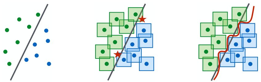
Figure 3: A conceptual illustration of standard vs. adversarial decision boundaries. Left: A set of points that can be easily separated with a simple (in this case, linear) decision boundary. Middle: The simple decision boundary does not separate the -balls (here, squares) around the data points. Hence there are adversarial examples (the red stars) that will be misclassified. Right: Separating the -balls requires a significantly more complicated decision boundary. The resulting classifier is robust to adversarial examples with bounded -norm perturbations.
图 3:标准决策边界与对抗决策边界的概念示意。左:一组可用简单(此处为线性)决策边界轻易分开的点。中:简单决策边界无法分隔数据点周围的 球(此处为正方形)。因此存在将被误分类的对抗样本(红星)。右:分隔 球需要显著更复杂的决策边界。所得分类器对有界 范数扰动的对抗样本鲁棒。
Our experiments verify that capacity is crucial for robustness, as well as for the ability to successfully train against strong adversaries. For the MNIST dataset, we consider a simple convolutional network and study how its behavior changes against different adversaries as we keep doubling the size of network (i.e. double the number of convolutional filters and the size of the fully connected layer). The initial network has a convolutional layer with 2 filters, followed by another convolutional layer with 4 filters, and a fully connected hidden layer with 64 units. Convolutional layers are followed by max-pooling layers and adversarial examples are constructed with . The results are in Figure 4.
实验验证容量对鲁棒性至关重要,对能否成功针对强对手训练亦然。对 MNIST,我们考虑简单卷积网络,并研究在不断把网络规模加倍(即卷积滤波器数与全连接层大小加倍)时,其面对不同对手的行为如何变化。初始网络有一层含 2 个滤波器的卷积,后接一层含 4 个滤波器的卷积,以及含 64 单元的全连接隐层。卷积层后接 最大池化;对抗样本以 构造。结果见图 4。
For the CIFAR10 dataset, we used a ResNet model [13]. We performed data augmentation using random crops and flips, as well as per image standarization. To increase the capacity, we modified the network incorporating wider layers by a factor of 10. This results in a network with 5 residual units with (16, 160, 320, 640) filters each. This network can achieve an accuracy of 95.2% when trained with natural examples. Adversarial examples were constructed with . Results on capacity experiments appear in Figure 4.
对 CIFAR10,我们使用 ResNet 模型[13]。数据增强包括随机裁剪与翻转,以及逐图像标准化。为增大容量,我们把各层加宽 10 倍,得到含 5 个残差单元、滤波器数分别为 (16, 160, 320, 640) 的网络。该网络在自然样本上训练可达 95.2% 准确率。对抗样本以 构造。容量实验结果见图 4。
We observe the following phenomena:
我们观察到以下现象:
Capacity alone helps.
We observe that increasing the capacity of the network when training using only natural examples (apart from increasing accuracy on these examples) increases the robustness against one-step perturbations. This effect is greater when considering adversarial examples with smaller .
仅容量本身就有帮助。
我们观察到:仅用自然样本训练时增大网络容量(除提高这些样本上的准确率外)也会增强对单步扰动的鲁棒性。在考虑较小 的对抗样本时,该效应更大。
FGSM adversaries don’t increase robustness (for large ).
When training the network using adversarial examples generated with the FGSM, we observe that the network overfits to these adversarial examples. This behavior is known as label leaking [18] and stems from the fact that the adversary produces a very restricted set of adversarial examples that the network can overfit to. These networks have poor performance on natural examples and don’t exhibit any kind of robustness against PGD adversaries. For the case of smaller the loss is ofter linear enough in the -ball around natural examples, that FGSM finds adversarial examples close to those found by PGD thus being a reasonable adversary to train against.
FGSM 对手不会提升鲁棒性(对大 )。
用 FGSM 生成的对抗样本训练网络时,我们观察到网络过拟合这些对抗样本。该行为被称为标签泄漏[18],源于对手只产生网络能够过拟合的非常受限的对抗样本集合。这些网络在自然样本上表现差,对 PGD 对手也不展现任何鲁棒性。对较小 ,自然样本周围 球内损失往往足够线性,使 FGSM 找到的对抗样本接近 PGD 找到的,从而成为合理的训练对手。
Weak models may fail to learn non-trivial classifiers.
In the case of small capacity networks, attempting to train against a strong adversary (PGD) prevents the network from learning anything meaningful. The network converges to always predicting a fixed class, even though it could converge to an accurate classifier through standard training. The small capacity of the network forces the training procedure to sacrifice performance on natural examples in order to provide any kind of robustness against adversarial inputs.
弱模型可能学不到非平凡分类器。
对小容量网络,试图针对强对手(PGD)训练会阻止网络学到任何有意义的东西。网络收敛到总是预测固定类别,尽管通过标准训练它本可收敛到准确分类器。网络的小容量迫使训练过程牺牲自然样本上的性能,才能对对抗输入提供任何形式的鲁棒性。
The value of the saddle point problem decreases as we increase the capacity.
Fixing an adversary model, and training against it, the value of (2.1) drops as capacity increases, indicating the the model can fit the adversarial examples increasingly well.
鞍点问题的值随容量增大而下降。
固定对手模型并针对它训练时,(2.1)的值随容量增大而下降,表明模型能越来越好拟合对抗样本。
More capacity and stronger adversaries decrease transferability.
Either increasing the capacity of the network, or using a stronger method for the inner optimization problem reduces the effectiveness of transferred adversarial inputs. We validate this experimentally by observing that the correlation between gradients from the source and the transfer network, becomes less significant as capacity increases. We describe our experiments in Section B of the appendix.
更大容量与更强对手降低可迁移性。
增大网络容量,或对内层优化问题使用更强方法,都会降低迁移对抗输入的有效性。我们通过观察源网络与迁移网络梯度之间的相关性随容量增大而减弱,在实验上验证了这一点。实验描述见附录 B。

| MNIST | |||||||||||||||||||||||||||||||||||||||
|---|---|---|---|---|---|---|---|---|---|---|---|---|---|---|---|---|---|---|---|---|---|---|---|---|---|---|---|---|---|---|---|---|---|---|---|---|---|---|---|
| Capacity scaleAccuracy | Capacity scale | Capacity scale | Capacity scaleAverage lossNaturalFGSMPGD | ||||||||||||||||||||||||||||||||||||
| CIFAR10 | |||||||||||||||||||||||||||||||||||||||
| Simple Wide Natural 92.7% 95.2% FGSM 27.5% 32.7% PGD 0.8% 3.5% | Simple | Wide | Natural | 92.7% | 95.2% | FGSM | 27.5% | 32.7% | PGD | 0.8% | 3.5% | Simple Wide 87.4% 90.3% 90.9% 95.1% 0.0% 0.0% | Simple | Wide | 87.4% | 90.3% | 90.9% | 95.1% | 0.0% | 0.0% | Simple Wide 79.4% 87.3% 51.7% 56.1% 43.7% 45.8% | Simple | Wide | 79.4% | 87.3% | 51.7% | 56.1% | 43.7% | 45.8% | Simple Wide 0.00357 0.00371 0.0115 0.00557 1.11 0.0218 | Simple | Wide | 0.00357 | 0.00371 | 0.0115 | 0.00557 | 1.11 | 0.0218 | |
| Simple | Wide | ||||||||||||||||||||||||||||||||||||||
| Natural | 92.7% | 95.2% | |||||||||||||||||||||||||||||||||||||
| FGSM | 27.5% | 32.7% | |||||||||||||||||||||||||||||||||||||
| PGD | 0.8% | 3.5% | |||||||||||||||||||||||||||||||||||||
| Simple | Wide | ||||||||||||||||||||||||||||||||||||||
| 87.4% | 90.3% | ||||||||||||||||||||||||||||||||||||||
| 90.9% | 95.1% | ||||||||||||||||||||||||||||||||||||||
| 0.0% | 0.0% | ||||||||||||||||||||||||||||||||||||||
| Simple | Wide | ||||||||||||||||||||||||||||||||||||||
| 79.4% | 87.3% | ||||||||||||||||||||||||||||||||||||||
| 51.7% | 56.1% | ||||||||||||||||||||||||||||||||||||||
| 43.7% | 45.8% | ||||||||||||||||||||||||||||||||||||||
| Simple | Wide | ||||||||||||||||||||||||||||||||||||||
| 0.00357 | 0.00371 | ||||||||||||||||||||||||||||||||||||||
| 0.0115 | 0.00557 | ||||||||||||||||||||||||||||||||||||||
| 1.11 | 0.0218 | ||||||||||||||||||||||||||||||||||||||
| (a) Standard training | (b) FGSM training | (c) PGD training | (d) Training Loss |
| Simple | Wide | |
|---|---|---|
| Natural | 92.7% | 95.2% |
| FGSM | 27.5% | 32.7% |
| PGD | 0.8% | 3.5% |
| Simple | Wide |
|---|---|
| 87.4% | 90.3% |
| 90.9% | 95.1% |
| 0.0% | 0.0% |
| Simple | Wide |
|---|---|
| 79.4% | 87.3% |
| 51.7% | 56.1% |
| 43.7% | 45.8% |
| Simple | Wide |
|---|---|
| 0.00357 | 0.00371 |
| 0.0115 | 0.00557 |
| 1.11 | 0.0218 |
Figure 4: The effect of network capacity on the performance of the network. We trained MNIST and CIFAR10 networks of varying capacity on: (a) natural examples, (b) with FGSM-made adversarial examples, (c) with PGD-made adversarial examples. In the first three plots/tables of each dataset, we show how the standard and adversarial accuracy changes with respect to capacity for each training regime. In the final plot/table, we show the value of the cross-entropy loss on the adversarial examples the networks were trained on. This corresponds to the value of our saddle point formulation (2.1) for different sets of allowed perturbations.
图 4:网络容量对网络性能的影响。我们在以下设定下训练不同容量的 MNIST 与 CIFAR10 网络:(a) 自然样本;(b) 用 FGSM 对抗样本;(c) 用 PGD 对抗样本。每个数据集的前三组图/表展示各训练体制下标准与对抗准确率如何随容量变化。最后一组图/表给出网络所训练对抗样本上的交叉熵损失值,对应我们鞍点形式(2.1)在不同允许扰动集合下的取值。
5 Experiments: Adversarially Robust Deep Learning Models
5 实验:对抗鲁棒的深度学习模型
Following the understanding of the problem we developed in previous sections, we can now apply our proposed approach to train robust classifiers. As our experiments so far demonstrated, we need to focus on two key elements: a) train a sufficiently high capacity network, b) use the strongest possible adversary.
顺着前几节对问题形成的理解,我们现在可以应用所提方法训练鲁棒分类器。至此实验表明,需要抓住两个关键要素:a) 训练容量足够高的网络;b) 使用尽可能强的对手。
For both MNIST and CIFAR10, the adversary of choice will be projected gradient descent (PGD) starting from a random perturbation around the natural example. This corresponds to our notion of a "complete" first-order adversary, an algorithm that can efficiently maximize the loss of an example using only first order information. Since we are training the model for multiple epochs, there is no benefit from restarting PGD multiple times per batch—a new start will be chosen the next time each example is encountered.
对 MNIST 与 CIFAR10,所选对手都是从自然样本周围的随机扰动起步的投影梯度下降(PGD)。这对应我们所谓「完备」一阶对手——仅用一阶信息就能高效最大化样本损失的算法。由于我们训练多个 epoch,每个 batch 对 PGD 多次重启动并无益处——下次遇到每个样本时会选择新的起点。
When training against that adversary, we observe a steady decrease in the training loss of adversarial examples, illustrated in Figure 5. This behavior indicates that we are indeed successfully solving our original optimization problem during training.
针对该对手训练时,我们观察到对抗样本上的训练损失稳步下降,如图 5 所示。这一行为表明我们在训练中确实成功求解了原始优化问题。
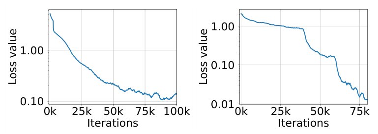
| (a) MNIST | (b) CIFAR10 |
Figure 5: Cross-entropy loss on adversarial examples during training. The plots show how the adversarial loss on training examples evolves during training the MNIST and CIFAR10 networks against a PGD adversary. The sharp drops in the CIFAR10 plot correspond to decreases in training step size. These plots illustrate that we can consistently reduce the value of the inner problem of the saddle point formulation (2.1), thus producing an increasingly robust classifier.
(a) MNIST (b) CIFAR10
图 5:训练期间对抗样本上的交叉熵损失。图中展示针对 PGD 对手训练 MNIST 与 CIFAR10 网络时,训练样本上对抗损失如何演化。CIFAR10 图中的急剧下降对应训练步长减小。这些图说明我们能持续降低鞍点形式(2.1)内层问题的值,从而得到日益鲁棒的分类器。
We evaluate the trained models against a range of adversaries. We illustrate our results in Table 1 for MNIST and Table 2 for CIFAR10. The adversaries we consider are:
我们针对一系列对手评估训练好的模型。MNIST 结果见表 1,CIFAR10 见表 2。我们考虑的对手是:
- • White-box attacks with PGD for a different number of of iterations and restarts, denoted by source A.
- • White-box attacks with PGD using the Carlini-Wagner (CW) loss function [6] (directly optimizing the difference between correct and incorrect logits). This is denoted as CW, where the corresponding attack with a high confidence parameter () is denoted as CW+.
- • Black-box attacks from an independently trained copy of the network, denoted A’.
- • Black-box attacks from a version of the same network trained only on natural examples, denoted .
- • Black-box attacks from a different convolution architecture, denoted B, described in Tramer et al. 2017 [29].
- • 不同迭代次数与重启动次数的白盒 PGD 攻击,源记为 A。
- • 使用 Carlini-Wagner(CW)损失函数[6]的白盒 PGD 攻击(直接优化正确与错误 logit 之差)。记为 CW;带高置信参数()的对应攻击记为 CW+。
- • 来自独立训练副本网络的黑盒攻击,记为 A’。
- • 来自仅在自然样本上训练的同结构网络版本的黑盒攻击,记为 。
- • 来自不同卷积结构的黑盒攻击,记为 B,结构见 Tramer 等人 2017 [29]。
MNIST.
We run 40 iterations of projected gradient descent as our adversary, with a step size of (we choose to take gradient steps in the -norm, i.e. adding the sign of the gradient, since this makes the choice of the step size simpler). We train and evaluate against perturbations of size . We use a network consisting of two convolutional layers with 32 and 64 filters respectively, each followed by max-pooling, and a fully connected layer of size 1024. When trained with natural examples, this network reaches 99.2% accuracy on the evaluation set. However, when evaluating on examples perturbed with FGSM the accuracy drops to 6.4%. The resulting adversarial accuracies are reported in Table 1. Given that the resulting MNIST model is very robust to -bounded adversaries, we investigated the learned parameters in order to understand how they affect adversarial robustness. The results of the investigation are presented in Appendix C. In particular, we found that the first convolutional layer of the network is learning to threshold input pixels while other weights tend to be sparser.
MNIST。
我们以 40 次投影梯度下降迭代作为对手,步长 (选择在 范数下迈梯度步,亦即加上梯度的符号,使步长选择更简单)。我们针对大小 的扰动训练与评估。所用网络由两个分别含 32 与 64 个滤波器的卷积层组成,每层后接 最大池化,以及大小为 1024 的全连接层。仅用自然样本训练时,该网络在评估集上达到 99.2% 准确率;但在 FGSM 扰动样本上评估时准确率降至 6.4%。所得对抗准确率见表 1。鉴于所得 MNIST 模型对 有界对手非常鲁棒,我们检查学到的参数以理解它们如何影响对抗鲁棒性。调查结果见附录 C。尤其是,我们发现网络的第一卷积层在学习对输入像素做阈值,而其他权重往往更稀疏。
| Method | Steps | Restarts | Source | Accuracy |
|---|---|---|---|---|
| Natural | - | - | - | 98.8% |
| FGSM | - | - | A | 95.6% |
| PGD | 40 | 1 | A | 93.2% |
| PGD | 100 | 1 | A | 91.8% |
| PGD | 40 | 20 | A | 90.4% |
| PGD | 100 | 20 | A | 89.3% |
| Targeted | 40 | 1 | A | 92.7% |
| CW | 40 | 1 | A | 94.0% |
| CW+ | 40 | 1 | A | 93.9% |
| FGSM | - | - | A’ | 96.8% |
| PGD | 40 | 1 | A’ | 96.0% |
| PGD | 100 | 20 | A’ | 95.7% |
| CW | 40 | 1 | A’ | 97.0% |
| CW+ | 40 | 1 | A’ | 96.4% |
| FGSM | - | - | B | 95.4% |
| PGD | 40 | 1 | B | 96.4% |
| CW+ | - | - | B | 95.7% |
Table 1: MNIST: Performance of the adversarially trained network against different adversaries for . For each model of attack we show the most successful attack with bold. The source networks used for the attack are: the network itself (A) (white-box attack), an indepentenly initialized and trained copy of the network (A’), architecture B from [29] (B).
表 1:MNIST:对抗训练网络在 下面对不同对手的表现。对每种攻击模型,最成功的攻击以粗体标出。攻击所用源网络为:网络自身(A)(白盒攻击)、独立初始化并训练的副本(A’)、[29] 中的结构 B(B)。
CIFAR10.
For the CIFAR10 dataset, we use the two architectures described in 4 (the original ResNet and its wider variant). We trained the network against a PGD adversary with projected gradient descent again, this time using 7 steps of size 2, and a total . For our hardest adversary we chose 20 steps with the same settings, since other hyperparameter choices didn’t offer a significant decrease in accuracy. The results of our experiments appear in Table 2.
CIFAR10。
对 CIFAR10,我们使用第 4 节描述的两种结构(原始 ResNet 及其 加宽变体)。我们再次针对 投影梯度下降的 PGD 对手训练网络,这次使用大小为 2 的 7 步,总 。对我们最强的对手,我们在相同设置下选用 20 步,因为其他超参选择并未显著降低准确率。实验结果见表 2。
| Method | Steps | Source | Accuracy |
|---|---|---|---|
| Natural | - | - | 87.3% |
| FGSM | - | A | 56.1% |
| PGD | 7 | A | 50.0% |
| PGD | 20 | A | 45.8% |
| CW | 30 | A | 46.8% |
| FGSM | - | A’ | 67.0% |
| PGD | 7 | A’ | 64.2% |
| CW | 30 | A’ | 78.7% |
| FGSM | - | 85.6% | |
| PGD | 7 | 86.0% |
Table 2: CIFAR10: Performance of the adversarially trained network against different adversaries for . For each model of attack we show the most effective attack in bold. The source networks considered for the attack are: the network itself (A) (white-box attack), an independtly initialized and trained copy of the network (A’), a copy of the network trained on natural examples ().
表 2:CIFAR10:对抗训练网络在 下面对不同对手的表现。对每种攻击模型,最有效的攻击以粗体标出。攻击所用源网络为:网络自身(A)(白盒攻击)、独立初始化并训练的副本(A’)、在自然样本上训练的副本()。
The adversarial robustness of our network is significant, given the power of iterative adversaries, but still far from satisfactory. We believe that these results can be improved by further pushing along these directions, and training networks of larger capacity.
鉴于迭代对手的威力,我们网络的对抗鲁棒性已相当可观,但仍远未令人满意。我们相信,沿着这些方向继续推进并训练更大容量的网络,结果还能改善。
Resistance for different values of and -bounded attacks.
In order to perform a broader evaluation of the adversarial robustness of our models, we run two additional experiments. On one hand, we investigate the resistance to -bounded attacks for different values of . On the other hand, we examine the resistance of our model to attacks that are bounded in -norm as opposed to -norm. In the case of -bounded PGD we take steps in the gradient direction (not the sign of it) and normalize the steps to be of fixed norm to facilitate step size tuning. For all PGD attacks, we use steps and set the step size to be to ensure that we can reach the boundary of the -ball from any starting point within it (and still allow for movement on the boundary). Note that the models were training against -bounded attacks with the original value of , for MNIST, and for CIFAR10. The results appear in Figure 6.
对不同 取值以及 有界攻击的抵抗。
为更广泛评估模型的对抗鲁棒性,我们再做两组实验。一方面,考察对不同 取值的 有界攻击的抵抗;另一方面,考察模型对 范数有界(而非 )攻击的抵抗。对 有界 PGD,我们沿梯度方向迈步(而非取其符号),并把步长归一化为固定范数以便调参。对所有 PGD 攻击,我们使用 步,并把步长设为 ,以确保从球内任意起点都能到达 球边界(并仍允许在边界上移动)。注意模型是针对原始 取值的 有界攻击训练的:MNIST 为 ,CIFAR10 为 。结果见图 6。

| Accuracy | PGD adv. trainedDBA adv. trainedPGD standardDBA standard | ||
|---|---|---|---|
| (a) MNIST, -norm | (b) MNIST, -norm | (c) CIFAR10, -norm | (d) CIFAR10, -norm |
Figure 6: Performance of our adversarially trained networks against PGD adversaries of different strength. The MNIST and CIFAR10 networks were trained against and PGD adversaries respectively (the training is denoted with a red dashed lines in the plots). In the case of the MNIST adversarially trained networks, we also evaluate the performance of the Decision Boundary Attack (DBA) [4] with 2000 steps and PGD on standard and adversarially trained models. We observe that for less or equal to the value used during training, the performance is equal or better. For MNIST there is a sharp drop shortly after. Moreover, we observe that the performance of PGD on the MNIST -trained networks is poor and significantly overestimates the robustness of the model. This is potentially due to the threshold filters learned by the model masking the loss gradients (the decision-based attack does not utilize gradients).
(a) MNIST, 范数 (b) MNIST, 范数 (c) CIFAR10, 范数 (d) CIFAR10, 范数
图 6:我们的对抗训练网络面对不同强度 PGD 对手时的表现。MNIST 与 CIFAR10 网络分别针对 与 的 PGD 对手训练(训练 在 图中以红色虚线标出)。对 MNIST 对抗训练网络,我们还评估 2000 步的决策边界攻击(DBA)[4],以及标准与对抗训练模型上的 PGD。我们观察到:对小于或等于训练所用取值的 ,性能持平或更好;对 MNIST,略大后出现急剧下降。此外,PGD 在 MNIST 训练网络上的表现很差,显著高估了模型鲁棒性。这可能因为模型学到的阈值滤波器屏蔽了损失梯度(基于决策的攻击不利用梯度)。
We observe that for smaller than the one used during training the models achieve equal or higher accuracy, as expected. For MNIST, we notice a large drop in robustness for slightly large values, potentially due to the fact that the threshold operators learned are tuned to the exact value of used during training (Appendix C). In contrast, the decay for the case of CIFAR10 is smoother.
我们观察到:对小于训练所用取值的 ,模型准确率如预期地持平或更高。对 MNIST,略大的 就会使鲁棒性大幅下降,可能因为学到的阈值算子被调到训练时所用的精确 值(附录 C)。相比之下,CIFAR10 上的衰减更平滑。
For the case of -bounded attacks on MNIST, we observe that PGD is unable to find adversarial examples even for quite large values of , e.g., . To put this value of into perspective, we provide a sample of corresponding adversarial examples in Figure 12 of Appendix D. We observe that these perturbations are significant enough that they would change the ground-truth label of the images and it is thus unlikely that our models are actually that robust. Indeed, subsequent work [20, 25] has found that PGD is in fact overestimating the -robustness of this model. This behavior is potentially due to the fact that the learned threshold filters (Appendix C) mask the gradient, preventing PGD from maximizing the loss. Attacking the model with a decision-based attack [4] which does not rely on model gradients reveals that the model is significantly more brittle against -bounded attacks. Nevertheless, the -trained model is still more robust to attacks compared to a standard model.
对 MNIST 上的 有界攻击,我们观察到即便 相当大(例如 ),PGD 仍找不到对抗样本。为把该 取值放到语境中,附录 D 图 12 给出对应对抗样本示例。我们观察到这些扰动已大到足以改变图像的真实标签,因此模型不太可能真有那么高的鲁棒性。的确,后续工作[20, 25]发现 PGD 实际上高估了该模型的 鲁棒性。这一行为可能因为学到的阈值滤波器(附录 C)屏蔽了梯度,阻止 PGD 最大化损失。用不依赖模型梯度的基于决策的攻击[4]攻击该模型,揭示其对 有界攻击要脆弱得多。尽管如此,相对标准模型, 训练模型对 攻击仍然更鲁棒。
6 Related Work
6 相关工作
Due to the large body of work on adversarial examples we focus only on the most related papers here. Before we compare our contributions, we remark that robust optimization has been studied outside deep learning for multiple decades (see [1] for an overview of this field). We also want to note that the study of adversarial ML predates the widespread use of deep neural networks [8, 10] (see [3] for an overview of earlier work).
由于对抗样本文献庞大,此处只聚焦最相关的论文。在比较我们的贡献之前,我们指出鲁棒优化在深度学习之外已被研究数十年(该领域综述见[1])。我们也想指出,对抗机器学习的研究早于深度神经网络的广泛使用[8, 10](早期工作综述见[3])。
Adversarial training was introduced in [11], however the adversary utilized was quite weak—it relied on linearizing the loss around the data points. As a result, while these models were robust against this particular adversary, they were completely vulnerable to slightly more sophisticated adversaries utilizing iterative attacks.
对抗训练在[11]中被提出,但所用对手相当弱——它依赖在数据点附近线性化损失。结果是,这些模型对该特定对手鲁棒,却对利用迭代攻击的稍复杂对手完全脆弱。
Recent work on adversarial training on ImageNet also observed that the model capacity is important for adversarial training [18]. In contrast to this paper, we find that training against multi-step methods (PGD) does lead to resistance against such adversaries.
近期 ImageNet 上的对抗训练工作也观察到模型容量对对抗训练很重要[18]。与该文不同,我们发现针对多步方法(PGD)训练确实带来对此类对手的抵抗。
In [15] and [26] a version of the min-max optimization problem is also considered for adversarial training. There are, however, three important differences between the formerly mentioned result and the present paper. Firstly, the authors claim that the inner maximization problem can be difficult to solve, whereas we explore the loss surface in more detail and find that randomly re-started projected gradient descent often converges to solutions with comparable quality. This shows that it is possible to obtain sufficiently good solutions to the inner maximization problem, which offers good evidence that deep neural network can be immunized against adversarial examples. Secondly, they consider only one-step adversaries, while we work with multi-step methods. Additionally, while the experiments in [26] produce promising results, they are only evaluated against FGSM. However, FGSM-only evaluations are not fully reliable. One evidence for that is that [26] reports 70% accuracy for , but any adversary that is allowed to perturb each pixel by more than 0.5 can construct a uniformly gray image, thus fooling any classifier.
[15] 与 [26] 也为对抗训练考虑了某种 min-max 优化问题。不过前述结果与本文有三点重要差异。首先,作者声称内层最大化可能很难求解,而我们更细致地探索损失曲面,发现随机重启动的投影梯度下降往往收敛到质量可比的解。这表明有可能为内层最大化获得足够好的解,从而为深度神经网络可被免疫对抗样本提供良好证据。其次,他们只考虑单步对手,而我们使用多步方法。此外,尽管[26]的实验给出有希望的结果,它们只对 FGSM 评估。然而仅用 FGSM 的评估并不完全可靠。证据之一是[26]对 报告 70% 准确率,但任何被允许把每个像素扰动超过 0.5 的对手都能构造均匀灰色图像,从而愚弄任何分类器。
A more recent paper [29] also explores the transferability phenomenon. This exploration focuses mostly on the region around natural examples where the loss is (close to) linear. When large perturbations are allowed, this region does not give a complete picture of the adversarial landscape. This is confirmed by our experiments, as well as pointed out by [29].
更新近的论文[29]也探索可迁移性现象。该探索主要聚焦自然样本周围损失(接近)线性的区域。当允许大扰动时,该区域并不能给出对抗景观的完整图景。我们的实验证实了这一点,[29]也指出了这一点。
7 Conclusion
7 结论
Our findings provide evidence that deep neural networks can be made resistant to adversarial attacks. As our theory and experiments indicate, we can design reliable adversarial training methods. One of the key insights behind this is the unexpectedly regular structure of the underlying optimization task: even though the relevant problem corresponds to the maximization of a highly non-concave function with many distinct local maxima, their values are highly concentrated. Overall, our findings give us hope that adversarially robust deep learning models may be within current reach.
我们的发现为深度神经网络可被做成抵抗对抗攻击提供了证据。正如理论与实验所表明的,我们可以设计可靠的对抗训练方法。背后的关键洞见之一是底层优化任务出人意料地规整的结构:尽管相关问题对应高度非凹函数的最大化,且有许多不同的局部极大值,它们的取值却高度集中。总体而言,这些发现让我们有希望:对抗鲁棒的深度学习模型或许已在当前可及范围内。
For the MNIST dataset, our networks are very robust, achieving high accuracy for a wide range of powerful -bound adversaries and large perturbations. Our experiments on CIFAR10 have not reached the same level of performance yet. However, our results already show that our techniques lead to significant increase in the robustness of the network. We believe that further exploring this direction will lead to adversarially robust networks for this dataset.
对 MNIST,我们的网络非常鲁棒,对广泛的强 有界对手与大扰动都达到高准确率。CIFAR10 上的实验尚未达到同等水平。但结果已表明我们的技术显著提升了网络鲁棒性。我们相信继续探索这一方向将为该数据集带来对抗鲁棒网络。
Acknowledgments
致谢
Aleksander Mądry, Aleksandar Makelov, and Dimitris Tsipras were supported by the NSF Grant No. 1553428, a Google Research Fellowship, and a Sloan Research Fellowship. Ludwig Schmidt was supported by a Google PhD Fellowship. Adrian Vladu was supported by the NSF Grants No. 1111109 and No. 1553428.
Aleksander Mądry、Aleksandar Makelov 与 Dimitris Tsipras 得到 NSF Grant No. 1553428、Google Research Fellowship 与 Sloan Research Fellowship 的支持。Ludwig Schmidt 得到 Google PhD Fellowship 的支持。Adrian Vladu 得到 NSF Grants No. 1111109 与 No. 1553428 的支持。
We thank Wojciech Matusik for kindly providing us with computing resources to perform this work.
感谢 Wojciech Matusik 慷慨提供完成本工作所需的计算资源。
References
参考文献
[1] Aharon Ben-Tal, Laurent El Ghaoui, and Arkadi Nemirovski. Robust optimization . Princeton University Press, 2009.
[2] Battista Biggio, Igino Corona, Davide Maiorca, Blaine Nelson, Nedim Šrndić, Pavel Laskov, Giorgio Giacinto, and Fabio Roli. Evasion attacks against machine learning at test time. In Joint European conference on machine learning and knowledge discovery in databases (ECML-KDD) , 2013.
[3] Battista Biggio and Fabio Roli. Wild patterns: Ten years after the rise of adversarial machine learning. 2018.
[4] Wieland Brendel, Jonas Rauber, and Matthias Bethge. Decision-based adversarial attacks: Reliable attacks against black-box machine learning models. In International Conference on Learning Representations (ICLR) , 2017.
[5] Nicholas Carlini and David Wagner. Adversarial examples are not easily detected: Bypassing ten detection methods. In Workshop on Artificial Intelligence and Security (AISec) , 2017.
[6] Nicholas Carlini and David Wagner. Towards evaluating the robustness of neural networks. In Symposium on Security and Privacy (SP) , 2017.
[7] Ronan Collobert and Jason Weston. A unified architecture for natural language processing: Deep neural networks with multitask learning. In Proceedings of the 25th international conference on Machine learning , pages 160–167, 2008.
[8] Nilesh Dalvi, Pedro Domingos, Sumit Sanghai, and Deepak Verma. Adversarial classification. In international conference on Knowledge discovery and data mining , 2004.
[9] Alhussein Fawzi, Omar Fawzi, and Pascal Frossard. Analysis of classifiers’ robustness to adversarial perturbations. Machine Learning , 107(3):481–508, 2018.
[10] Amir Globerson and Sam Roweis. Nightmare at test time: robust learning by feature deletion. In Proceedings of the 23rd international conference on Machine learning , 2006.
[11] Ian J Goodfellow, Jonathon Shlens, and Christian Szegedy. Explaining and harnessing adversarial examples. In International Conference on Learning Representations (ICLR) , 2015.
[12] Kaiming He, Xiangyu Zhang, Shaoqing Ren, and Jian Sun. Delving deep into rectifiers: Surpassing human-level performance on imagenet classification. In international conference on computer vision (ICCV) , 2015.
[13] Kaiming He, Xiangyu Zhang, Shaoqing Ren, and Jian Sun. Deep residual learning for image recognition. In Conference on Computer Vision and Pattern Recognition (CVPR) , 2016.
[14] Warren He, James Wei, Xinyun Chen, Nicholas Carlini, and Dawn Song. Adversarial example defense: Ensembles of weak defenses are not strong. In USENIX Workshop on Offensive Technologies (WOOT) , 2017.
[15] Ruitong Huang, Bing Xu, Dale Schuurmans, and Csaba Szepesvari. Learning with a strong adversary. arXiv preprint arXiv:1511.03034 , 2015.
[16] Alex Krizhevsky. Learning multiple layers of features from tiny images. In Technical report , 2009.
[17] Alex Krizhevsky, Ilya Sutskever, and Geoffrey E Hinton. Imagenet classification with deep convolutional neural networks. In Advances in Neural Information Processing Systems (NeurIPS) , 2012.
[18] Alexey Kurakin, Ian J. Goodfellow, and Samy Bengio. Adversarial machine learning at scale. In International Conference on Learning Representations (ICLR) , 2017.
[19] Yann LeCun. The mnist database of handwritten digits. In Technical report , 1998.
[20] Bai Li, Changyou Chen, Wenlin Wang, and Lawrence Carin. Second-order adversarial attack and certifiable robustness. arXiv preprint arXiv:1809.03113 , 2018.
[21] Seyed-Mohsen Moosavi-Dezfooli, Alhussein Fawzi, and Pascal Frossard. Deepfool: a simple and accurate method to fool deep neural networks. In Computer Vision and Pattern Recognition (CVPR) , 2016.
[22] Anh Nguyen, Jason Yosinski, and Jeff Clune. Deep neural networks are easily fooled: High confidence predictions for unrecognizable images. In Conference on computer vision and pattern recognition (CVPR) , 2015.
[23] Nicolas Papernot, Patrick McDaniel, and Ian Goodfellow. Transferability in machine learning: from phenomena to black-box attacks using adversarial samples. In ArXiv preprint arXiv:1605.07277 , 2016.
[24] Nicolas Papernot, Patrick D. McDaniel, Xi Wu, Somesh Jha, and Ananthram Swami. Distillation as a defense to adversarial perturbations against deep neural networks. In Symposium on Security and Privacy (SP) , 2016.
[25] Lukas Schott, Jonas Rauber, Matthias Bethge, and Wieland Brendel. Towards the first adversarially robust neural network model on MNIST. In International Conference on Learning Representations (ICLR) , 2019.
[26] Uri Shaham, Yutaro Yamada, and Sahand Negahban. Understanding adversarial training: Increasing local stability of supervised models through robust optimization. Neurocomputing , 307:195–204, 2018.
[27] Jure Sokolić, Raja Giryes, Guillermo Sapiro, and Miguel RD Rodrigues. Robust large margin deep neural networks. In Transactions on Signal Processing , 2017.
[28] Christian Szegedy, Wojciech Zaremba, Ilya Sutskever, Joan Bruna, Dumitru Erhan, Ian Goodfellow, and Rob Fergus. Intriguing properties of neural networks. In International Conference on Learning Representations (ICLR) , 2014.
[29] Florian Tramer, Nicolas Papernot, Ian Goodfellow, and Patrick McDaniel Dan Boneh. The space of transferable adversarial examples. In ArXiv preprint arXiv:1704.03453 , 2017.
[30] Abraham Wald. Statistical decision functions which minimize the maximum risk. In Annals of Mathematics , 1945.
[31] Weilin Xu, David Evans, and Yanjun Qi. Feature squeezing: Detecting adversarial examples in deep neural networks. In Network and Distributed Systems Security Symposium (NDSS) , 2018.
Appendix A Statement and Application of Danskin’s Theorem
附录 A Danskin 定理的陈述与应用
Recall that our goal is to minimize the value of the saddle point problem
回顾我们的目标是最小化鞍点问题的值
In practice, we don’t have access to the distribution so both the gradients and the value of will be computed using sampled input points. Therefore we can consider –without loss of generality– the case of a single random example with label , in which case the problem becomes
实践中我们无法访问分布 ,因此 的梯度与取值都用采样输入点计算。于是我们可以不失一般性地考虑单个随机样本 与标签 的情形,此时问题变为
If we assume that the loss is continuously differentiable in , we can compute a descent direction for by utilizing the classical theorem of Danskin.
若假设损失 对 连续可微,我们可利用 Danskin 的经典定理计算 的下降方向。
Theorem A.1(Danskin).
Let be nonempty compact topological space and be such that is differentiable for every and is continuous on . Also, let $\delta^{}(\theta)={\delta\in\arg\max_{\delta\in\mathcal{S}}g(\theta,\delta)}$.*
定理 A.1(Danskin)。
设 为非空紧拓扑空间, 满足:对每个 , 可微,且 在 上连续。又设 $\delta^{}(\theta)={\delta\in\arg\max_{\delta\in\mathcal{S}}g(\theta,\delta)}$。*
Then the corresponding max-function
则对应的极大函数
is locally Lipschitz continuous, directionally differentiable, and its directional derivatives satisfy
局部 Lipschitz 连续、方向可微,且其方向导数满足
In particular, if for some the set $\delta^{}(\theta)={\delta^{}_{\theta}}\theta$ and
尤其是,若对某个 ,集合 $\delta^{}(\theta)={\delta^{}_{\theta}}\theta$ 可微,且
The intuition behind the theorem is that since gradients are local objects, and the function is locally the same as their gradients will be the same. The theorem immediately gives us the following corollary, stating the we can indeed compute gradients for the saddle point by computing gradients at the inner optimizers.
定理背后的直觉是:梯度是局部对象,而函数 在局部与 相同,因而它们的梯度相同。定理立刻给出如下推论:我们确实可以通过在内层优化子处计算梯度来得到鞍点的梯度。
Corollary A.2.
Let be such that and is a maximizer for . Then, as long as it is nonzero, is a descent direction for .
推论 A.2。
设 满足 且是 的极大化子。则只要它非零, 就是 的下降方向。
Proof of Corollary A.2.
We apply Theorem A.1 to and . We see that the directional derivative in the direction of satisfies
推论 A.2 的证明。
我们对 与 应用定理 A.1。可见沿方向 的方向导数满足
If this gradient is nonzero, then the inequality above is strict. Therefore it gives a descent direction. ∎
若该梯度非零,则上述不等式是严格的。因此它给出下降方向。∎
A technical issue is that, since we use ReLU and max-pooling units in our neural network architecture, the loss function is not continuously differentiable. Nevertheless, since the set of discontinuities has measure zero, we can assume that this will not be an issue in practice, as we will never encounter the problematic points.
一个技术问题是:由于网络结构中使用 ReLU 与最大池化单元,损失函数并非连续可微。不过,不连续集合测度为零,我们可以假定实践中不会成为问题,因为我们不会遇到这些麻烦点。
Another technical issue is that, due to the not concavity of the inner problem, we are not able to compute global maximizers, since PGD will converge to local maxima. In such cases, we can consider a subset of such that the local maximum is a global maximum in the region . Applying the theorem for gives us that the gradient corresponds to a descent direction for the saddle point problem when the adversary is constrained in . Therefore if the inner maximum is a true adversarial example for the network, then SGD using the gradient at that point will decrease the loss value at this particular adversarial examples, thus making progress towards a robust model.
另一技术问题是:由于内层问题非凹,我们无法计算全局极大化子,因为 PGD 会收敛到局部极大。此时可考虑 的子集 ,使该局部极大在区域 内是全局极大。对 应用定理可得:当对手被约束在 时,梯度对应鞍点问题的下降方向。因此,若内层极大确是网络的真实对抗样本,则在该点用梯度做 SGD 会降低该特定对抗样本上的损失值,从而朝鲁棒模型推进。
These arguments suggest that the conclusions of the theorem are still valid in our saddle point problem, and –as our experiments confirm– we can solve it reliably.
这些论证表明定理结论对我们的鞍点问题仍然成立——正如实验所确认——我们能可靠求解它。
Appendix B Transferability
附录 B 可迁移性
A lot of recent literature on adversarial training discusses the phenomenon of transferability [28, 11, 29]—adversarial examples transfer between independently trained networks. This raises concerns for practical applications, since it suggests that deep networks are vulnerable to attacks, even when there is no direct access to the target network.
近期大量对抗训练文献讨论可迁移性现象[28, 11, 29]——对抗样本在独立训练的网络之间迁移。这对实际应用提出担忧,因为它表明即便无法直接访问目标网络,深度网络仍易受攻击。
This phenomenon is further confirmed by our current experiments. [^2] Moreover, we notice that the extent to which adversarial examples transfer decreases as we increase either network capacity or the power of the adversary used for training the network. This serves as evidence for the fact that the transferability phenomenon can be alleviated by using high capacity networks in conjunction with strong oracles for the inner optimization problem.
当前实验进一步证实了这一现象。[^2] 此外我们注意到:增大网络容量或增强训练所用对手的强度,都会降低对抗样本迁移的程度。这为如下事实提供证据:结合高容量网络与内层优化问题的强 oracle,可缓解可迁移性现象。
MNIST.
In an attempt to understand these phenomena we inspect the loss functions corresponding to the trained models we used for testing transferability. More precisely, we compute angles between gradients of the loss functions evaluated over a large set of input examples, and plot their distribution. Similarly, we plot the value of the loss functions between clean and perturbed examples for both the source and transfer networks. In Figure 8 we plot our experimental findings on the MNIST dataset for . We consider a large standard network (two convolutional layers of sizes and , and a fully connected layer of size ), which we train twice starting with different initializations. We plot the distribution of angles between gradients for the same test image in the two resulting networks ( orange histograms), noting that they are somewhat correlated. As opposed to this, we see that pairs of gradients for random pairs of inputs for one architecture are as uncorrelated as they can be ( blue histograms), since the distribution of their angles looks Gaussian.
MNIST。
为理解这些现象,我们检查用于测试可迁移性的已训练模型所对应的损失函数。更精确地,我们在大量输入样本上计算损失函数梯度之间的夹角,并画出其分布。类似地,我们画出源网络与迁移网络上干净样本与扰动样本之间的损失值。图 8 给出 MNIST 上 的实验结果。我们考虑大型标准网络(两个大小为 与 的卷积层,以及大小为 的全连接层),从不同初始化起步训练两次。我们画出两网络对同一测试图像梯度夹角的分布(橙色直方图),并注意到它们有一定相关。与此相对,同一结构上随机输入对的梯度对几乎完全不相关(蓝色直方图),因为其夹角分布看起来像高斯。
Next, we run the same experiment on a very large standard network (two convolutional layers of sizes and , and a fully connected layer of size ). We notice a mild increase in classification accuracy for transferred examples.
接下来,我们在非常大的标准网络(两个大小为 与 的卷积层,以及大小为 的全连接层)上做同一实验。我们注意到迁移样本上的分类准确率有轻度提升。
Finally, we repeat the same set of experiments, after training the large and very large networks against the FGSM adversary. We notice that gradients between the two architectures become significantly less correlated. Also, the classification accuracy for transferred examples increases significantly compared to the standard networks.
最后,在针对 FGSM 对手训练大网络与非常大网络之后,我们重复同一组实验。我们注意到两种结构之间的梯度相关性显著下降。同时,迁移样本上的分类准确率相对标准网络显著上升。
We further plot how the value of the loss function changes when moving from the natural input towards the adversarially perturbed input (in Figure 8 we show these plots for four images in the MNIST test dataset), for each pair of networks we considered. We observe that, while for the naturally trained networks, when moving towards the perturbed point, the value of the loss function on the transfer architecture tends to start increasing soon after it starts increasing on the source architecture. In contrast, for the stronger models, the loss function on the transfer network tends to start increasing later, and less aggressively.
我们进一步画出从自然输入移向对抗扰动输入时损失函数取值如何变化(图 8 给出 MNIST 测试集四幅图像上的这些图),对考虑的每对网络皆然。我们观察到:对自然训练网络,朝扰动点移动时,迁移结构上的损失往往在源结构开始上升后不久也开始上升。相比之下,对更强模型,迁移网络上的损失往往更晚、且更不激进地开始上升。
CIFAR10.
For the CIFAR10 dataset, we investigate the transferability of the FGSM and PGD adversaries between our simple and wide architectures, each trained on natural, FGSM and PGD examples. Transfer accuracies for the FGSM adversary and PGD adversary between all pairs of such configurations (model + training method) with independently random weight initialization are given in tables 3 and 4 respectively. The results exhibit the following trends:
CIFAR10。
对 CIFAR10,我们考察 FGSM 与 PGD 对手在简单与加宽结构之间的可迁移性;每种结构分别在自然、FGSM 与 PGD 样本上训练。独立随机权重初始化下,所有此类配置(模型 + 训练方法)对之间的 FGSM 与 PGD 对手迁移准确率分别见表 3 与表 4。结果呈现如下趋势:
- • Stronger adversaries decrease transferability: In particular, transfer attacks between two PGD-trained models are less successful than transfer attacks between their standard counterparts. Moreover, adding PGD training helps with transferability from all adversarial datasets, except for those with source a PGD-trained model themselves. This applies to both FGSM attacks and PGD attacks.
- • Capacity decreases transferability: In particular, transfer attacks between two PGD-trained wide networks are less successful than transfer attacks between their simple PGD-trained counterparts. Moreover, with few close exceptions, changing the architecture from simple to wide (and keeping the training method the same) helps with transferability from all adversarial datasets.
- • 更强对手降低可迁移性: 尤其是,两个 PGD 训练模型之间的迁移攻击不如其标准对应物之间成功。此外,加入 PGD 训练有助于抵御来自所有对抗数据集的迁移,除非源本身就是 PGD 训练模型。这对 FGSM 攻击与 PGD 攻击都成立。
- • 容量降低可迁移性: 尤其是,两个 PGD 训练加宽网络之间的迁移攻击不如其简单 PGD 训练对应物之间成功。此外,除少数接近的例外外,把结构从简单改为加宽(训练方法不变)有助于抵御来自所有对抗数据集的迁移。
We additionally plotted how the loss of a network behaves in the direction of FGSM and PGD examples obtained from itself and an independently trained copy; results for the simple standard network and the wide PGD trained network are given in Table 7. As expected, we observe the following phenomena:
我们还画出网络损失沿来自自身与独立训练副本的 FGSM、PGD 样本方向如何变化;简单标准网络与加宽 PGD 训练网络的结果见表 7。如预期,我们观察到以下现象:
- • sometimes, the FGSM adversary manages to increase loss faster near the natural example, but as we move towards the boundary of the box of radius , the PGD attack always achieves higher loss.
- • the transferred attacks do worse than their white-box counterparts in terms of increasing the loss;
- • and yet, the transferred PGD attacks dominate the white-box FGSM attacks for the standard network (and sometimes for the PGD-trained one too).
- • 有时 FGSM 对手能在自然样本附近更快抬高损失,但当我们移向半径 的 盒边界时,PGD 攻击总是达到更高损失。
- • 迁移攻击在抬高损失方面逊于其白盒对应物;
- • 尽管如此,对标准网络,迁移 PGD 攻击仍主导白盒 FGSM 攻击(有时对 PGD 训练网络亦然)。
| Simple (standard training) | Simple | (standard | training) | Simple (FGSM training) | Simple | (FGSM | training) | Simple (PGD training) | Simple | (PGD | training) | Wide (natural training) | Wide | (natural | training) | Wide (FGSM training) | Wide | (FGSM | training) | Wide (PGD training) | Wide | (PGD | training) | |
|---|---|---|---|---|---|---|---|---|---|---|---|---|---|---|---|---|---|---|---|---|---|---|---|---|
| Simple | ||||||||||||||||||||||||
| (standard | ||||||||||||||||||||||||
| training) | ||||||||||||||||||||||||
| Simple | ||||||||||||||||||||||||
| (FGSM | ||||||||||||||||||||||||
| training) | ||||||||||||||||||||||||
| Simple | ||||||||||||||||||||||||
| (PGD | ||||||||||||||||||||||||
| training) | ||||||||||||||||||||||||
| Wide | ||||||||||||||||||||||||
| (natural | ||||||||||||||||||||||||
| training) | ||||||||||||||||||||||||
| Wide | ||||||||||||||||||||||||
| (FGSM | ||||||||||||||||||||||||
| training) | ||||||||||||||||||||||||
| Wide | ||||||||||||||||||||||||
| (PGD | ||||||||||||||||||||||||
| training) | ||||||||||||||||||||||||
| Simple (standard training) | Simple | (standard training) | 32.9% | 74.0% | 73.7% | 27.6% | 71.8% | 76.6% | ||||||||||||||||
| Simple | ||||||||||||||||||||||||
| (standard training) | ||||||||||||||||||||||||
| Simple (FGSM training) | Simple | (FGSM training) | 64.2% | 90.7% | 60.9% | 61.5% | 90.2% | 67.3% | ||||||||||||||||
| Simple | ||||||||||||||||||||||||
| (FGSM training) | ||||||||||||||||||||||||
| Simple (PGD training) | Simple | (PGD training) | 77.1% | 78.1% | 60.2% | 77.0% | 77.9% | 66.3% | ||||||||||||||||
| Simple | ||||||||||||||||||||||||
| (PGD training) | ||||||||||||||||||||||||
| Wide (standard training) | Wide | (standard training) | 34.9% | 78.7% | 80.2% | 21.3% | 75.8% | 80.6% | ||||||||||||||||
| Wide | ||||||||||||||||||||||||
| (standard training) | ||||||||||||||||||||||||
| Wide (FGSM training) | Wide | (FGSM training) | 64.5% | 93.6% | 69.1% | 53.7% | 92.2% | 72.8% | ||||||||||||||||
| Wide | ||||||||||||||||||||||||
| (FGSM training) | ||||||||||||||||||||||||
| Wide (PGD training) | Wide | (PGD training) | 85.8% | 86.6% | 73.3% | 85.6% | 86.2% | 67.0% | ||||||||||||||||
| Wide | ||||||||||||||||||||||||
| (PGD training) |
| Simple |
|---|
| (standard |
| training) |
| Simple |
|---|
| (FGSM |
| training) |
| Simple |
|---|
| (PGD |
| training) |
| Wide |
|---|
| (natural |
| training) |
| Wide |
|---|
| (FGSM |
| training) |
| Wide |
|---|
| (PGD |
| training) |
| Simple |
|---|
| (standard training) |
| Simple |
|---|
| (FGSM training) |
| Simple |
|---|
| (PGD training) |
| Wide |
|---|
| (standard training) |
| Wide |
|---|
| (FGSM training) |
| Wide |
|---|
| (PGD training) |
Table 3: CIFAR10: black-box FGSM attacks. We create FGSM adversarial examples with from the evaluation set on the source network, and then evaluate them on an independently initialized target network.
表 3:CIFAR10:黑盒 FGSM 攻击。我们在源网络上用评估集构造 的 FGSM 对抗样本,再在独立初始化的目标网络上评估它们。
| Simple (standard training) | Simple | (standard | training) | Simple (FGSM training) | Simple | (FGSM | training) | Simple (PGD training) | Simple | (PGD | training) | Wide (natural training) | Wide | (natural | training) | Wide (FGSM training) | Wide | (FGSM | training) | Wide (PGD training) | Wide | (PGD | training) | |||
|---|---|---|---|---|---|---|---|---|---|---|---|---|---|---|---|---|---|---|---|---|---|---|---|---|---|---|
| Simple | ||||||||||||||||||||||||||
| (standard | ||||||||||||||||||||||||||
| training) | ||||||||||||||||||||||||||
| Simple | ||||||||||||||||||||||||||
| (FGSM | ||||||||||||||||||||||||||
| training) | ||||||||||||||||||||||||||
| Simple | ||||||||||||||||||||||||||
| (PGD | ||||||||||||||||||||||||||
| training) | ||||||||||||||||||||||||||
| Wide | ||||||||||||||||||||||||||
| (natural | ||||||||||||||||||||||||||
| training) | ||||||||||||||||||||||||||
| Wide | ||||||||||||||||||||||||||
| (FGSM | ||||||||||||||||||||||||||
| training) | ||||||||||||||||||||||||||
| Wide | ||||||||||||||||||||||||||
| (PGD | ||||||||||||||||||||||||||
| training) | ||||||||||||||||||||||||||
| Simple (standard training) | Simple | (standard training) | 6.6% | 71.6% | 71.8% | 1.4% | 51.4% | 75.6% | ||||||||||||||||||
| Simple | ||||||||||||||||||||||||||
| (standard training) | ||||||||||||||||||||||||||
| Simple (FGSM training) | Simple | (FGSM training) | 66.3% | 40.3% | 58.4% | 65.4% | 26.8% | 66.2% | ||||||||||||||||||
| Simple | ||||||||||||||||||||||||||
| (FGSM training) | ||||||||||||||||||||||||||
| Simple (PGD training) | Simple | (PGD training) | 78.1% | 78.2% | 57.7% | 77.9% | 78.1% | 65.2% | ||||||||||||||||||
| Simple | ||||||||||||||||||||||||||
| (PGD training) | ||||||||||||||||||||||||||
| Wide (standard training) | Wide | (standard training) | 10.9% | 79.6% | 79.1% | 0.0% | 51.3% | 79.7% | ||||||||||||||||||
| Wide | ||||||||||||||||||||||||||
| (standard training) | ||||||||||||||||||||||||||
| Wide (FGSM training) | Wide | (FGSM training) | 67.6% | 51.7% | 67.4% | 56.5% | 0.0% | 71.6% | ||||||||||||||||||
| Wide | ||||||||||||||||||||||||||
| (FGSM training) | ||||||||||||||||||||||||||
| Wide (PGD training) | Wide | (PGD training) | 86.4% | 86.8% | 72.1% | 86.0% | 86.3% | 64.2% | ||||||||||||||||||
| Wide | ||||||||||||||||||||||||||
| (PGD training) |
| Simple |
|---|
| (standard |
| training) |
| Simple |
|---|
| (FGSM |
| training) |
| Simple |
|---|
| (PGD |
| training) |
| Wide |
|---|
| (natural |
| training) |
| Wide |
|---|
| (FGSM |
| training) |
| Wide |
|---|
| (PGD |
| training) |
| Simple |
|---|
| (standard training) |
| Simple |
|---|
| (FGSM training) |
| Simple |
|---|
| (PGD training) |
| Wide |
|---|
| (standard training) |
| Wide |
|---|
| (FGSM training) |
| Wide |
|---|
| (PGD training) |
Table 4: CIFAR10: black-box PGD attacks. We create PGD adversarial examples with for iterations from the evaluation set on the source network, and then evaluate them on an independently initialized target network.
表 4:CIFAR10:黑盒 PGD 攻击。我们在源网络上用评估集构造 、迭代 次的 PGD 对抗样本,再在独立初始化的目标网络上评估它们。
| Natural | FGSM | FGSM random | PGD (7 steps) | PGD (20 steps) | |||
|---|---|---|---|---|---|---|---|
| Simple (standard training) | Simple | (standard training) | 92.7% | 27.5% | 19.6% | 1.2% | 0.8% |
| Simple | |||||||
| (standard training) | |||||||
| Simple (FGSM training) | Simple | (FGSM training) | 87.4% | 90.9% | 90.4% | 0.0% | 0.0% |
| Simple | |||||||
| (FGSM training) | |||||||
| Simple (PGD training) | Simple | (PGD training) | 79.4% | 51.7% | 55.9% | 47.1% | 43.7% |
| Simple | |||||||
| (PGD training) | |||||||
| Wide (standard training) | Wide | (standard training) | 95.2% | 32.7% | 25.1% | 4.1% | 3.5% |
| Wide | |||||||
| (standard training) | |||||||
| Wide (FGSM training) | Wide | (FGSM training) | 90.3% | 95.1% | 95.0% | 0.0% | 0.0% |
| Wide | |||||||
| (FGSM training) | |||||||
| Wide (PGD training) | Wide | (PGD training) | 87.3% | 56.1% | 60.3% | 50.0% | 45.8% |
| Wide | |||||||
| (PGD training) |
| Simple |
|---|
| (standard training) |
| Simple |
|---|
| (FGSM training) |
| Simple |
|---|
| (PGD training) |
| Wide |
|---|
| (standard training) |
| Wide |
|---|
| (FGSM training) |
| Wide |
|---|
| (PGD training) |
Table 5: CIFAR10: white-box attacks for . For each architecture and training method, we list the accuracy of the resulting network on the full CIFAR10 evaluation set of 10,000 examples. The FGSM random method is the one suggested by [29], whereby we first do a small random perturbation of the natural example, and the apply FGSM to that.
表 5:CIFAR10:白盒攻击,。对每种结构与训练方法,我们列出所得网络在完整 CIFAR10 评估集(10,000 样本)上的准确率。FGSM random 方法由[29]建议:先对自然样本做小随机扰动,再对其施加 FGSM。
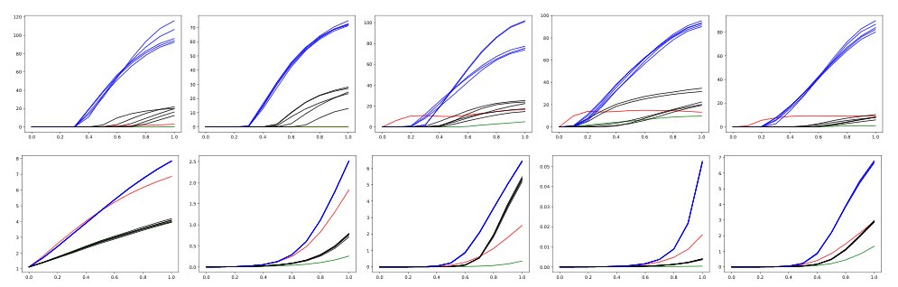
Figure 7: CIFAR10: change of loss function in the direction of white-box and black-box FGSM and PGD examples with for the same five natural examples. Each line shows how the loss changes as we move from the natural example to the corresponding adversarial example. Top: simple naturally trained model. Bottom: wide PGD trained model. We plot the loss of the original network in the direction of the FGSM example for the original network ( red lines), 5 PGD examples for the original network obtained from 5 random starting points ( blue lines), the FGSM example for an independently trained copy network ( green lines) and 5 PGD examples for the copy network obtained from 5 random starting points ( black lines). All PGD attacks use 100 steps with step size .
图 7:CIFAR10:对同一五个自然样本,损失沿白盒与黑盒 FGSM、PGD 样本方向()的变化。每条线展示从自然样本移向对应对抗样本时损失如何变化。上:简单自然训练模型。下:加宽 PGD 训练模型。我们画出原网络沿原网络 FGSM 样本方向的损失(红线)、原网络从 5 个随机起点得到的 5 个 PGD 样本方向(蓝线)、独立训练副本网络的 FGSM 样本方向(绿线),以及副本网络从 5 个随机起点得到的 5 个 PGD 样本方向(黑线)。所有 PGD 攻击使用 100 步,步长 。
| Source | Transfer | |
|---|---|---|
| Clean | 99.2% | 99.2% |
| FGSM | 3.9% | 41.9% |
| PGD | 0.0% | 26.0% |
| Source | Transfer | |
|---|---|---|
| Clean | 99.2% | 99.3% |
| FGSM | 7.2% | 44.6% |
| PGD | 0.0% | 35.0% |
| Source | Transfer | |
|---|---|---|
| Clean | 92.9% | 96.1% |
| FGSM | 99.9% | 62.0% |
| PGD | 0.0% | 54.1% |
| Source | Transfer | |
|---|---|---|
| Clean | 96.4% | 97.8% |
| FGSM | 99.4% | 71.6% |
| PGD | 0.0% | 60.6% |
Large network, standard training
大网络,标准训练
(MNIST 可迁移性对照表:干净 / FGSM / PGD 在源与迁移网络上的准确率;含标准训练与 FGSM 训练等设定。)
Appendix C MNIST Inspection
附录 C MNIST 检查
The robust MNIST model described so far is small enough that we can visually inspect most of its parameters. Doing so will allow us to understand how it is different from a standard network and what are the general characteristics of a network that is robust against adversaries. We will compare three different networks: a standard model, and two adversarially trained ones. The latter two models are identical, modulo the random weight initialization, and were used as the public and secret models used for our robustness challenge.
至此描述的鲁棒 MNIST 模型足够小,我们可以目视检查其大多数参数。这样做能让我们理解它与标准网络有何不同,以及对 对手鲁棒的网络有哪些一般特征。我们将比较三种网络:标准模型,以及两个对抗训练模型。后两者除随机权重初始化外完全相同,并分别用作我们鲁棒性挑战的公开模型与秘密模型。
Initially, we examine the first convolutional layer of each network. We observe that the robust models only utilize 3 out of the total 32 filters, and for each of these filters only one weight is non-zero. By doing so, the convolution degrades into a scaling of the original image. Combined with the bias and the ReLU that follows, this results in a thresholding filter, or equivalently for some constants , . From the perspective of adversarial robustness, thresholding filters are immune to any perturbations on pixels with value less than . We visualize a sample of the filters in Figure 9 (plots a, c, and e).
首先检查每个网络的第一卷积层。我们观察到鲁棒模型只利用总共 32 个滤波器中的 3 个,且每个滤波器只有一个权重非零。如此一来,卷积退化为对原图的缩放。再结合随后的偏置与 ReLU,结果是阈值滤波器,或等价地 (某些常数 ,)。从对抗鲁棒性视角,阈值滤波器对取值小于 的像素上的任何扰动都免疫。我们在图 9(图 a、c、e)可视化滤波器样本。
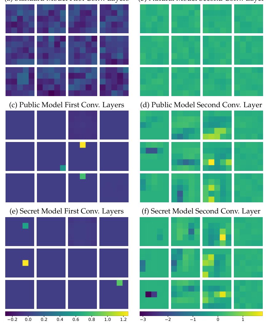
| (a) Standard Model First Conv. Layers | (b) Natural Model Second Conv. Layer |
|---|---|
| (c) Public Model First Conv. Layers | (d) Public Model Second Conv. Layer |
| (e) Secret Model First Conv. Layers | (f) Secret Model Second Conv. Layer |
Figure 9: Visualizing a sample of the convolutional filters. For the standard model (a,b) we visualize random filters, since there is no observable difference in any of them. For the first layer of robust networks we make sure to include the 3 non-zero filters. For the second layer, the first three columns represent convolutional filters that utilize the 3 non-zero channels, and we choose the most interesting ones (larger range of values). We observe that adversarially trained networks have significantly more concentrated weights. Moreover, the first convolutional layer degrades into a few thresholding filters.
(a) 标准模型第一卷积层 (b) 自然模型第二卷积层
(c) 公开模型第一卷积层 (d) 公开模型第二卷积层
(e) 秘密模型第一卷积层 (f) 秘密模型第二卷积层
图 9:卷积滤波器样本可视化。对标准模型 (a,b) 我们可视化随机滤波器,因为它们之间看不出可观察差异。对鲁棒网络的第一层,我们确保纳入 3 个非零滤波器。对第二层,前三列表示利用这 3 个非零通道的卷积滤波器,我们选取最有趣者(取值范围更大)。我们观察到对抗训练网络的权重显著更集中。此外,第一卷积层退化成少数阈值滤波器。
Having observed that the first layer of the network essentially maps the original image to three copies thresholded at different values, we examine the second convolutional layer of the classifier. Again, the filter weights are relatively sparse and have a significantly wider value range than the standard version. Since only three channels coming out of the first layer matter, is follows (and is verified) that the only relevant convolutional filters are those that interact with these three channels. We visualize a sample of the filters in Figure 9 (plots b, d, and f).
观察到网络第一层本质上把原图映射为在不同取值处阈值的三份拷贝后,我们检查分类器的第二卷积层。同样,滤波器权重相对稀疏,取值范围显著宽于标准版本。由于第一层出来只有三个通道重要,随之而来(并被验证)的是:只有与这三通道交互的卷积滤波器才相关。我们在图 9(图 b、d、f)可视化滤波器样本。
Finally, we examine the softmax/output layer of the network. While the weights seem to be roughly similar between all three version of the network, we notice a significant difference in the class biases. The adversarially trained networks heavily utilize class biases (far from uniform), and do so in a way very similar to each other. A plausible explanation is that certain classes tend to be very vulnerable to adversarial perturbations, and the network learns to be more conservative in predicting them. The plots can be found in Figure 10.
最后检查网络的 softmax/输出层。尽管三种网络版本的权重看起来大致相似,我们注意到类别偏置有显著差异。对抗训练网络大量利用类别偏置(远非均匀),且彼此方式非常相似。一种可信解释是:某些类别对对抗扰动特别脆弱,网络学会在预测它们时更保守。图见 图 10。
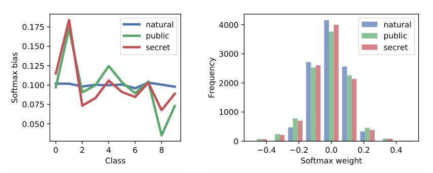
| (a) Softmax biases for each class | (b) Distribution of softmax weights |
Figure 10: Softmax layer examination. For each network we create a histogram of the layer’s weights and plot the per-class bias. We observe that while weights are similar (slightly more concentrated for the standard one) the biases are far from uniform and with a similar pattern for the two adversarially trained networks.
(a) 各类别的 Softmax 偏置 (b) Softmax 权重分布
图 10:Softmax 层检查。对每个网络我们创建该层权重的直方图,并画出逐类偏置。我们观察到权重相似(标准网络略更集中),但偏置远非均匀,且两个对抗训练网络模式相似。
All of the “tricks” described so far seem intuitive to a human and would seem reasonable directions when trying to increase the adversarial robustness of a classifier. We emphasize the none of these modifications were hard-coded in any way and they were all learned solely through adversarial training. We attempted to manually introduce these modifications ourselves, aiming to achieve adversarial robustness without adversarial training, but with no success. A simple PGD adversary could fool the resulting models on all the test set examples.
至此描述的所有「技巧」对人来说都显得直观,在试图提升分类器对抗鲁棒性时也像合理方向。我们强调:这些改动无一以任何方式被硬编码,全部仅通过对抗训练学到。我们曾尝试手动引入这些改动,目标是在不做对抗训练的情况下获得对抗鲁棒性,但未成功。简单的 PGD 对手就能在全部测试集样本上愚弄所得模型。
Appendix D Supplementary Figures
附录 D 补充图
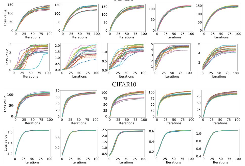
| MNIST | ||||
|---|---|---|---|---|
| CIFAR10 | ||||
Figure 11: Loss function value over PGD iterations for 20 random restarts on random examples. The 1st and 3rd rows correspond to standard networks, while the 2nd and 4th to adversarially trained ones.
图 11:随机样本上 20 次随机重启动的 PGD 迭代过程中的损失值。第 1、3 行对应标准网络,第 2、4 行对应对抗训练网络。
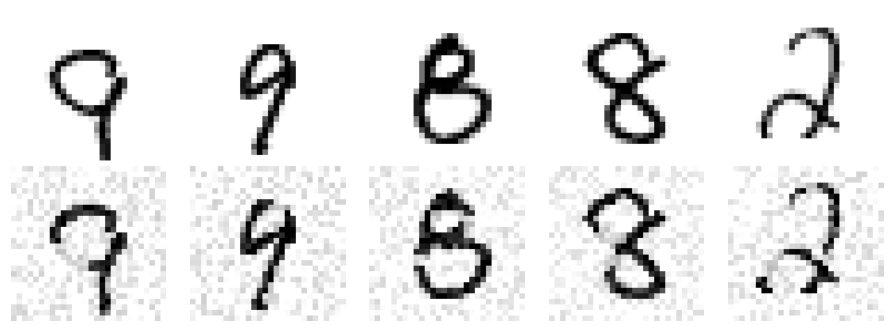
| Natural: 9 | Natural: 9 | Natural: 8 | Natural: 8 | Natural: 2 |
| Adversarial: 7 | Adversarial: 4 | Adversarial: 5 | Adversarial: 3 | Adversarial: 3 |
Figure 12: Sample adversarial examples with norm bounded by . The perturbations are significant enough to cause misclassification by humans too.
图 12: 范数以 为界的对抗样本示例。扰动已大到足以让人类也误分类。