MAC-VO: Metrics-aware Covariance for Learning-based Stereo Visual Odometry
MAC-VO: Metrics-aware Covariance for Learning-based Stereo Visual Odometry mac-vo.github.io
MAC-VO:面向学习型双目视觉里程计的度量感知协方差
MAC-VO: Metrics-aware Covariance for Learning-based Stereo Visual Odometry mac-vo.github.io
Yuheng Qiu * Affiliation: Yuheng Qiu, Yutian Chen and Sebastian Scherer are with the Robotics Institute, Carnegie Mellon University, Pittsburgh, PA 15213, USA {yuhengq, yutianch, basti} @andrew.cmu.edu; Yutian Chen * Affiliation: Yuheng Qiu, Yutian Chen and Sebastian Scherer are with the Robotics Institute, Carnegie Mellon University, Pittsburgh, PA 15213, USA {yuhengq, yutianch, basti} @andrew.cmu.edu; Zihao Zhang Affiliation: Zi hao Zhang is with the School of Ocean and Civil Engineering, Shanghai JiaoTong University, Shanghai 20024, China zihao6061@gmail.com Wenshan Wang Affiliation: Yuheng Qiu, Yutian Chen and Sebastian Scherer are with the Robotics Institute, Carnegie Mellon University, Pittsburgh, PA 15213, USA {yuhengq, yutianch, basti} @andrew.cmu.edu; Sebastian Scherer † † thanks: * Equal contribution. † † thanks: This work was supported by the DSTA under contract number #DST000EC124000205. Affiliation: Yuheng Qiu, Yutian Chen and Sebastian Scherer are with the Robotics Institute, Carnegie Mellon University, Pittsburgh, PA 15213, USA {yuhengq, yutianch, basti} @andrew.cmu.edu;
Abstract
摘要
We propose MAC-VO, a novel learning-based stereo visual odometry (VO) framework that trains a metrics-aware uncertainty model to serve two critical functions: selecting keypoints and weighting residuals in pose graph optimization. Unlike traditional geometric methods that favor texture-rich features like edges, our keypoint selector leverages this learned uncertainty model to eliminate low-quality features based on global inconsistency. In contrast to learning-based approaches that rely on scale-agnostic weight matrices for covariance, our metrics-aware covariance model—derived from the learned uncertainty—captures spatial errors in keypoint registration and inter-axis correlations. By embedding this covariance model into pose graph optimization, MAC-VO achieves superior robustness and accuracy in pose estimation, excelling in challenging environments with varying illumination, feature density, and motion patterns. Evaluations on public benchmark datasets demonstrate that MAC-VO surpasses existing VO algorithms and even some SLAM systems in difficult scenarios. Additionally, the uncertainty map offers valuable insights for decision-making.
我们提出 MAC-VO,这是一种学习型双目视觉里程计(visual odometry,VO)框架。它训练一个度量感知的不确定性模型,承担两项关键工作:挑选关键点,以及在位姿图优化中为残差加权。传统几何方法更偏向边缘这类纹理丰富的特征,而我们的关键点选择器利用学到的不确定性,按全局不一致性剔除低质量特征。学习方法通常用无尺度的权重矩阵当作协方差;与此不同,我们由学习到的不确定性导出度量感知协方差,用来刻画关键点配准的空间误差和轴间相关性。把这一协方差模型嵌入位姿图优化后,MAC-VO 在光照变化、特征疏密不一和运动模式多样的困难环境中,位姿估计更稳健、也更准确。公开基准上的评测表明,MAC-VO 超过了已有的 VO 算法,在困难场景里甚至超过部分 SLAM 系统。此外,不确定性图还能为后续决策提供参考。
I Introduction
I 引言
Index Terms:
Visual Odometry (VO) predicts the relative camera pose from image sequences and often serves as the front-end of Simultaneous Localization and Mapping (SLAM) systems. Over the past few decades, both geometric and learning-based methods have been developed with significant advances in generalizability and accuracy [1, 2, 3, 4]. However, VO remains a challenging problem in real-world scenarios, with multiple visually degraded scenarios such as low illumination, dynamic and texture-less scenes.
索引词:
视觉里程计(Visual Odometry,VO)根据图像序列估计相机的相对位姿,常常作为同时定位与地图构建(SLAM)系统的前端。过去几十年里,几何方法和学习方法都在泛化能力和精度上取得了明显进展[1, 2, 3, 4]。但在真实场景中,VO 仍然不好做,尤其是低光照、动态场景和缺少纹理这类视觉退化情况。
To improve the robustness in challenging scenes, geometric-based VO algorithms employ outlier filtering strategies [5] and weigh the optimization residuals by the covariance of the observed features [6]. However, how to effectively select the reliable keypoints and model their covariance becomes two significant challenges. Existing methods typically select the keypoints based on local intensity gradient with a manually defined threshold [7, 8, 9]. These approaches lead to errors and outliers because they don’t model the structure or context information of the environment (e.g., features on repetitive patterns may not be ideal candidates despite high image gradients). Moreover, the covariance model is often empirically modeled using a constant parameter, which is sub-optimal. In addition, the parameters in the keypoint selection and covariance model need to be extensively tuned for different environments.
为了在困难场景里提高稳健性,基于几何的 VO 会做外点过滤[5],并用观测特征的协方差给优化残差加权[6]。可是,怎样有效地选出可靠关键点,又怎样建模它们的协方差,仍是两个主要难点。现有方法通常按局部强度梯度、再配上手动阈值来选点[7, 8, 9]。这些做法不考虑环境的结构或上下文(例如重复纹理上的特征,尽管图像梯度很高,却不一定适合),因此容易引入误差和外点。协方差模型也常常用一个常数经验参数来写,并不理想。关键点选择和协方差里的参数,还往往要针对不同环境反复调节。
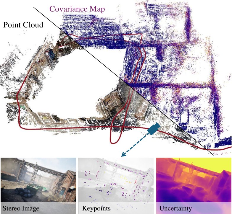
Fig. 1: Without relying on multi-frame bundle adjustment, MAC-VO aggregately reconstructs the map based on the two-frame Pose graph optimization. We propose metrics-aware covariance model for 3D keypoint based on the learning matching uncertainty.
图 1:MAC-VO 不依赖多帧光束法平差,而是基于两帧位姿图优化来聚合重建地图。我们根据学习到的匹配不确定性,为三维关键点提出度量感知协方差模型。
With advances in learning-based visual features, more algorithms utilize learned features [7] to optimize the camera pose. Confidence score [10] or confidence weights [3, 4] of these feature points are often obtained in an unsupervised manner. The learned confidence helps to track the features and model the reliability during the optimization. However, these confidence or uncertainty values are scale-agnostic, which means they don’t reflect the actual estimation error in the 3D space. This scale-agnostic problem brings two limitations. Firstly, it makes the covariance inconsistent across different environments that vary in scale, such as indoors and outdoors. Secondly, it makes it harder to integrate multiple constraints from different modalities or sensors.
随着学习型视觉特征的进步,越来越多算法用学到的特征[7]来优化相机位姿。这些特征点的置信分数[10]或置信权重[3, 4]常常以无监督方式得到。学到的置信度有助于跟踪特征,并在优化时刻画可靠性。不过,这些置信度或不确定性是无尺度的,并不能反映三维空间里真实的估计误差。无尺度带来两点限制。第一,协方差在室内外这类尺度不同的环境之间并不一致。第二,它更难把来自不同模态或传感器的多种约束整合到一起。
To overcome the above challenges, this paper addresses the problem of modeling metrics-aware covariance values for the 3D keypoints. More specifically, this is achieved through two innovations. Firstly, we propose a learning-based model to quantify the 2D metrics-aware uncertainty of feature matching. Inspired by the FlowFormer [11] and GMA [12], we employ an iterative update model and motion aggregator to predict the uncertainty in 2D image space, which helps to filter unreliable features in the occluded region or low-illumination area. Secondly, based on the learned 2D uncertainty values, we model the covariance of the feature points in 3D space using a metrics-aware 3D covariance model. Compared to DROID-SLAM [3], which utilizes a scale-agnostic diagonal covariance matrix, our approach provides a more accurate representation by modeling the covariance of 3D feature points. This covariance model includes the inter-axes correlation of the 3D features. In the ablation study, we demonstrate the inter-frame consistency and the intra-frame consistency of our proposed covariance model.
为克服上述困难,本文要解决的是为三维关键点建模度量感知协方差。具体来说有两项改进。第一,我们提出一个学习模型,用来量化特征匹配在二维上的度量感知不确定性。受 FlowFormer[11] 和 GMA[12] 启发,我们用迭代更新模型和运动聚合器预测二维图像空间中的不确定性,从而滤掉遮挡区域或低光照区域里不可靠的特征。第二,在学到的二维不确定性之上,我们用度量感知的三维协方差模型来描述特征点在三维空间中的协方差。DROID-SLAM[3] 使用无尺度的对角协方差矩阵;相比之下,我们的方法直接对三维特征点的协方差建模,并包含各轴之间的相关性。消融实验表明,该协方差模型同时具有帧间一致性和帧内一致性。
We integrate the above two innovations into MAC-VO, a stereo VO that features superior keypoint selection and pose graph optimization based on the metrics-aware covariance model and achieves accurate tracking results in challenging cases compared with state-of-the-art VOs and even some SLAM systems without fine-tuning and without multi-frame optimization. In summary, the main contributions are:
我们把上述两点改进放进 MAC-VO。这是一种双目 VO:它按度量感知协方差模型来做关键点选择和位姿图优化,无需微调、也不做多帧优化,就能在困难场景中取得比现有一流 VO、甚至部分 SLAM 系统更准确的跟踪结果。主要贡献如下:
- • We present a learning-based 2D uncertainty network with metrics awareness, leveraging an iterative motion aggregator to capture the inconsistency of the feature matching. We use this metrics-aware uncertainty to evaluate the quality of features, in order to select keypoints, and guide the backend optimization.
- • 我们提出具有度量感知能力的学习型二维不确定性网络,用迭代运动聚合器捕捉特征匹配的不一致性。我们用这种度量感知不确定性评价特征质量,以便挑选关键点,并指导后端优化。
- • This paper introduces a novel metrics-aware 3D covariance model based on the 2D uncertainty of feature matching and depth estimation. The ablation study demonstrates the necessity of scale consistency and the off-diagonal terms in the pose graph optimization.
- • 本文基于特征匹配和深度估计的二维不确定性,引入一种新的度量感知三维协方差模型。消融实验表明,位姿图优化需要尺度一致性以及非对角项。
- • We propose the MAC-VO, a stereo VO pipeline that estimates the camera pose and registers 3D features with metrics-aware covariance. In the experiments, MAC-VO outperforms existing VO algorithms even some SLAM algorithms in challenging environments.
- • 我们提出 MAC-VO,这是一条用度量感知协方差估计相机位姿并注册三维特征的双目 VO 流水线。实验中,MAC-VO 在困难环境里超过了已有 VO 算法,甚至超过部分 SLAM 算法。
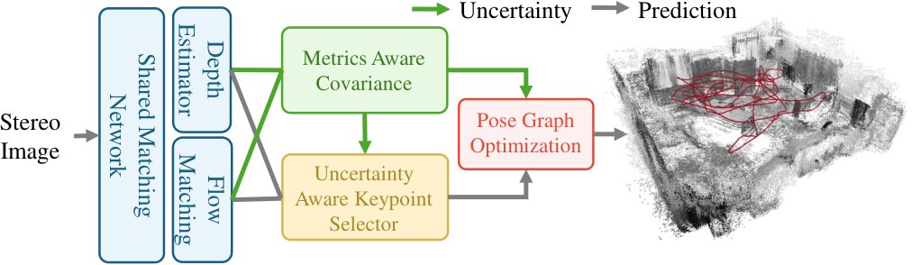
Fig. 2: MAC-VO pipeline. It employs a shared matching network to jointly estimate depth, optical flow, and corresponding uncertainties. The learned uncertainty is utilized in the keypoint selector, the metrics-aware 3D covariance model, and the back-end optimization.
图 2:MAC-VO 流水线。它用共享的匹配网络联合估计深度、光流及相应不确定性。学到的不确定性用于关键点选择器、度量感知三维协方差模型,以及后端优化。
II Related Works
II 相关工作
Existing geometric-based methods optimize the camera pose based on geometric constraints like re-projection error [1, 13] or photometric error [14, 15, 16]. To more accurately model the uncertainty of the depth, Civera et al. [17] and Montiel[18] investigate the inverse depth parameterization. These methods often use constant parameters and simple heuristics to model the covariance matrix of these errors during the factor graph optimization. For multi-sensor fusion [6, 19] and semantic SLAM [20, 21], the covariance model plays a significant role in weighting the confidence of different sensors and modules. To capture sensor uncertainty, the covariance models are often tuned based on empirical prior. However, these simplified covariance models fail to capture the complexity of the challenging environments.
现有的几何方法依据重投影误差[1, 13]或光度误差[14, 15, 16]这类几何约束来优化相机位姿。为了更准确地建模深度的不确定性,Civera 等人[17]和 Montiel[18]研究了逆深度参数化。这些方法在因子图优化中,常常用常数参数和简单启发式规则来写这些误差的协方差矩阵。在多传感器融合[6, 19]和语义 SLAM[20, 21]里,协方差模型对权衡不同传感器和模块的置信度很关键。为了刻画传感器不确定性,协方差模型往往按经验先验来调。不过,这些简化模型难以抓住困难环境的复杂性。
Recent advances in deep learning have transformed research in optical flow estimation [22, 23], feature matching [24, 10], depth estimation [25, 26, 27], and end-to-end camera pose estimation [28, 2]. Several methodologies have been developed to address the uncertainty in estimating depth, flow, and pose. Dexheimer et al. [29] proposed a learned depth covariance function that is applied in downstream tasks like 3D reconstruction. Nie et al. utilize a self-supervised learning method to jointly train depth and depth covariance of images in the wild [30]. ProbFlow [31] proposes using post-hoc confidence measures to assess the per-pixel reliability of flow.
深度学习近来改变了光流估计[22, 23]、特征匹配[24, 10]、深度估计[25, 26, 27]以及端到端相机位姿估计[28, 2]的研究。已有多种方法处理深度、光流和位姿估计中的不确定性。Dexheimer 等人[29]提出一种学习得到的深度协方差函数,并把它用到三维重建等下游任务。Nie 等人用自监督学习,对野外图像联合训练深度和深度协方差[30]。ProbFlow[31]则用事后置信度量来评估每个像素上光流的可靠性。
Amidst these developments, hybrid learning-based SLAM systems [32, 26, 33, 34, 35, 36] are emerging to synergize the geometric constraint with the adaptability of learning-based methods. To improve the reliability of the feature tracking process, some methods introduce learning-based uncertainty measurements or confidence scores [37, 38, 10, 39, 40] for pose optimization. DROID-SLAM [3] utilizes a differentiable bundle adjustment layer to implicitly tune the uncertainty model. This method employs a simplified diagonal covariance model for the bundle adjustment. These methods focus on the relative confidence between features, but ignore the scale consistency of the covariance model.
在这些进展之中,混合学习型 SLAM 系统[32, 26, 33, 34, 35, 36]正在把几何约束和学习方法的适应性结合起来。为了提高特征跟踪的可靠性,一些方法为位姿优化引入学习型不确定性度量或置信分数[37, 38, 10, 39, 40]。DROID-SLAM[3]用可微光束法平差层隐式调节不确定性模型,并在光束法平差中采用简化的对角协方差。这些方法关注的是特征之间的相对置信度,却忽略了协方差模型的尺度一致性。
For keypoint selection, geometric-based VO relies on hand-crafted features [8, 9], which detect the edges and corner points. The recent advance of the learning-based method train feature extractor in data-driven manner [7, 41]. However, these keypoint also prioritize the edge and corner features due to their data bias in the pre-training dataset. Recent works like D3VO [32] have shown that relying on edge and corner points can degrade state estimation, sometimes performing worse than random selectors [4]. The accuracy of learning-based feature matching and depth estimation algorithms is particularly compromised at object edges due to feature interpolation and the ambiguity in neural networks. In this work, we propose a keypoint selector based on learned uncertainty to filter out the unreliable features.
在关键点选择上,基于几何的 VO 依赖手工特征[8, 9],检测边缘和角点。近期的学习方法则以数据驱动方式训练特征提取器[7, 41]。不过,由于预训练数据中的偏差,这些关键点仍然优先选择边缘和角点。D3VO[32]等工作已经表明,依赖边缘和角点会损害状态估计,有时甚至不如随机选择器[4]。学习型特征匹配和深度估计算法在物体边缘处尤其容易出错,原因是特征插值以及神经网络中的歧义。本文提出一种基于学习不确定性的关键点选择器,用来滤除不可靠特征。
III Method
III 方法

Fig. 3: We include three filters: Non-minimum Suppression (NMS) filter, geometric filter, and uncertainty-based filter. In the KITTI dataset, the uncertainty filter implicitly filters out the unreliable feature matchings in the scene.
图 3:我们使用三种滤波器:非极小值抑制(NMS)滤波器、几何滤波器,以及基于不确定性的滤波器。在 KITTI 数据集上,不确定性滤波器会隐式滤掉场景中不可靠的特征匹配。
As illustrated in Fig. 2, MAC-VO outlines an effective integration of a learning-based front-end and a geometrically constrained back-end using the metrics-aware covariance model. In the front-end (Section III-A), we train an uncertainty-aware matching network to model the corresponding uncertainty stems from feature deficiencies. Utilizing the learned uncertainty, we develop a keypoint selector in Section III-B to choose reliable features. The metrics-aware 2D uncertainty is then propagated to the 3D space via the proposed covariance model in Section III-C. In the back-end optimization (Section III-D), we optimize the relative motion by minimizing the distance between registered keypoints weighted by the 3D covariance.
如图 2 所示,MAC-VO 用度量感知协方差模型,把学习型前端和受几何约束的后端有效结合在一起。在前端(第 III-A 节),我们训练一个感知不确定性的匹配网络,用来建模由特征缺陷引起的相应不确定性。利用学到的不确定性,我们在第 III-B 节设计关键点选择器,选出可靠特征。度量感知的二维不确定性再通过第 III-C 节提出的协方差模型传播到三维空间。在后端优化(第 III-D 节)中,我们按三维协方差加权,最小化已注册关键点之间的距离,从而优化相对运动。
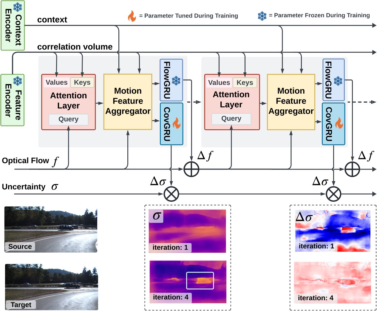
Fig. 4: Top: Architecture of the uncertainty-aware matching network. Bottom: Each iteration, the model captures the inconsistency of the matching. For the , the red color indicates a positive increasing the uncertainty, and blue means decreasing uncertainty.
图 4:上:感知不确定性的匹配网络结构。下:每次迭代中,模型捕捉匹配的不一致性。对 而言,红色表示正的 ,不确定性上升;蓝色表示不确定性下降。
III-A Network & Uncertainty Training
III-A 网络与不确定性训练
The objective of the proposed matching network is to estimate the flow and the corresponding uncertainty between two frames. We adopt the FlowFormer architecture [11] as the backbone for optical flow estimation, leveraging its transformer-based design. As shown in Fig. 4, the recurrent decoder iteratively refines flow predictions by capturing ambiguities in feature correspondence within the cost volume’s matching space, utilizing global context from the encoded cost memory.
所提出匹配网络的目标,是估计两帧之间的光流 以及相应的不确定性 。我们采用 FlowFormer 结构[11]作为光流估计的骨干,以利用其基于 Transformer 的设计。如图 4 所示,循环解码器借助编码后的代价记忆所提供的全局上下文,捕捉代价体匹配空间里特征对应关系的歧义,从而迭代地改进光流预测。
To extend this framework and leverages both global motion cues and local feature, we introduce a covariance decoder that predicts , the iterative updates of the uncertainty on log space. Operating the uncertainty update on the log space facilitates additive updates, ensures positive variances, and stabilizes gradients. After iterative updates, the log-variance passes through an exp activation function to obtain the final uncertainty. More details about the network and training are shown in Appendix B-E.
为了在这一框架上同时利用全局运动线索和局部特征,我们引入一个协方差解码器,预测 ,也就是对数空间中不确定性的迭代更新。在对数空间里更新不确定性,便于做加法更新,能保证方差为正,也让梯度更稳定。迭代更新之后,对数方差再经过 exp 激活,得到最终的不确定性。网络和训练的更多细节见附录 B-E。
To supervise the uncertainty, we leverage the negative log-likelihood loss used in conformal prediction [42, 43, 44]:
为了监督不确定性,我们采用共形预测中使用的负对数似然损失[42, 43, 44]:
where is the ground truth optical flow, denotes the -th iteration of the network outputs, and is the weight for each iteration and is set to decrease exponentially with a ratio of . During the training stage, we initialize the encoder network parameters with the pre-trained model by FlowFormer. We then train the covariance module on the synthetic dataset TartanAir [45], and evaluate the model in the TartanAirv2 sequences and other real-world datasets. Our experiments demonstrate that the model can generalize to real-world datasets without fine-tuning.
其中 是光流真值, 表示网络第 次迭代的输出, 是每次迭代的权重,并按 0.8 的比例指数递减。训练阶段,我们用 FlowFormer 的预训练模型初始化编码器参数,然后在合成数据集 TartanAir[45] 上训练协方差模块,并在 TartanAirv2 序列以及其他真实数据集上评估。实验表明,该模型无需微调即可泛化到真实数据。
III-B Uncertainty-based Keypoint Selection
III-B 基于不确定性的关键点选择
Different from the random selector used in DPVO[4] and the hand-crafted features selector used in ORB-SLAM [8], we leverage the learned uncertainty estimation to filter out unreliable features. This is achieved by composing three filters: the uncertainty filter, geometry filter, and the non-minimum suppression (NMS). To prevent the clustering of keypoint candidates, we first apply the NMS filter, ensuring a more even spatial distribution of features. The geometry filter further removes keypoints located at the image boundaries and those outside the valid depth observation range. Finally, the uncertainty filter eliminates pixels with depth and flow uncertainty greater than 1.5 times the median uncertainty of the current frame. Illustrated in Fig. 3, the uncertainty filter removes all keypoint candidates on the moving vehicle on a KITTI trajectory. Our proposed uncertainty estimation strategy also filters out keypoints on occluded objects, reflective surfaces, and feature-less areas, resulting in a more robust and reliable feature set.
不同于 DPVO[4] 使用的随机选择器,以及 ORB-SLAM[8] 使用的手工特征选择器,我们用学到的不确定性估计来滤除不可靠特征。这由三种滤波器组成:不确定性滤波器、几何滤波器和非极小值抑制(NMS)。为避免候选关键点挤成一团,我们先施加 NMS 滤波器,让特征在空间上分布更均匀。几何滤波器再去掉位于图像边界、以及落在有效深度观测范围之外的关键点。最后,不确定性滤波器剔除深度和光流不确定性大于当前帧中位不确定性 1.5 倍的像素。如图 3 所示,不确定性滤波器去掉了 KITTI 一条轨迹上移动车辆上的全部候选关键点。我们提出的不确定性估计策略还会滤掉遮挡物体、反射表面和缺少特征的区域上的关键点,从而得到更稳健、更可靠的特征集合。
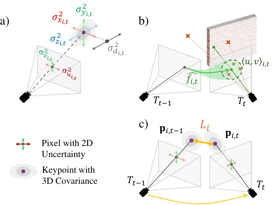
Fig. 5: a) Uncertain estimation of depth due to the error in feature matching. b) Projecting depth and matching uncertainty from image plane to 3D space. c) Residual for pose graph optimization.
图 5:a) 特征匹配误差导致的深度不确定性估计。b) 把深度和匹配不确定性从图像平面投影到三维空间。c) 位姿图优化的残差 。
III-C Metrics-aware 3D Covariance Model
III-C 度量感知的三维协方差模型
In the context of the camera projection geometry, the covariance of a 3D keypoint is determined by the uncertainty of the depth and matching . To accurately model the covariance for 3D keypoint, it is critical to determine (1) the depth uncertainty of the matched points and (2) the off-diagonal covariance terms during the 2D-3D projection.
在相机投影几何中,三维关键点的协方差由深度不确定性 和匹配不确定性 决定。要准确建模三维关键点的协方差,关键在于确定(1)匹配点的深度不确定性 ,以及(2)二维到三维投影过程中的非对角协方差项。
Project 2D Uncertainty to 3D Covariance Following the pinhole camera model with focal length and optical center , the coordinate of the keypoint is calculated by: , and , as shown in Fig. 5 (a). To accurately capture the uncertainties associated with these measurements, the main diagonal of the covariance matrix is formulated as:
把二维不确定性投影为三维协方差 按照焦距为 、光心为 的针孔相机模型,关键点坐标由 、 以及 算出,如图 5(a)所示。为准确刻画这些测量的不确定性,协方差矩阵的主对角线写为:
In this model, the projected coordinates are interdependent due to the common multiplier of depth . To precisely formulate the covariance of the 3D keypoints under camera coordinate, it is essential to include the off-diagonal covariance terms in .
在这个模型里,投影坐标因为共同乘上了深度 而彼此相关。要精确写出相机坐标系下三维关键点的协方差 ,必须在 中包含非对角协方差项。
$$\displaystyle{}^{c}\Sigma_{i,t}^{p}=\begin{bmatrix}\sigma_{z}^{2}&\sigma_{xz_{i,t}}&\sigma_{yz_{i,t}}\
\sigma_{xz_{i,t}}&\sigma_{x_{i,t}}^{2}&\sigma_{xy_{i,t}}\
\sigma_{yz_{i,t}}&\sigma_{xy_{i,t}}&\sigma_{y_{i,t}}^{2}\
\end{bmatrix}\begin{aligned} &\sigma_{xz}=\sigma_{d}^{2}(u-\mathrm{c}{x})/\mathrm{f}{x}\
&\sigma_{yz}=\sigma_{d}^{2}(v-\mathrm{c}{y})/\mathrm{f}{y}\
&\sigma_{xy}=\frac{\sigma_{d}^{2}(u-\mathrm{c}{x})(v-\mathrm{c}{y})}{\mathrm{f}{x}\mathrm{f}{y}}.\end{aligned}$$
Results in the ablation study also confirm the necessity of off-diagonal terms for accurate pose graph optimization. Detailed derivation for Eq. 2 and Eq. 3 is in Appendix A-C.
消融实验的结果也证实,非对角项对准确的位姿图优化是必要的。式 2 和式 3 的详细推导见附录 A-C。
Uncertainty Correction after Keypoint Matching As shown in Fig. 5 (b), the matched features are expected to fall in a probabilistic range centered at with the flow uncertainty . However, the depth observations of matched keypoints may vary due to scene geometry. For example, if a matched keypoint is located near the edge of an object, such as a wall, even a minor perturbation in feature matching can lead to substantial discrepancies in 3D keypoint registration. This, in turn, amplifies the uncertainty in the reconstructed 3D structure.
关键点匹配后的不确定性校正 如图 5(b)所示,匹配特征预期会落在以 为中心、由光流不确定性 决定的概率范围内。不过,由于场景几何的原因,匹配关键点上的深度观测可能不同。例如,若匹配关键点靠近墙壁这类物体的边缘,特征匹配上哪怕很小的扰动,也会在三维关键点注册时造成很大偏差,从而放大重建三维结构的不确定性。
To address this problem, we correct the depth uncertainty of the matched feature point based on the depth feature of the local patch with the kernel size of . We approximate it with the weighted sum of the variances within the patch. The weights are determined by a 2D Gaussian kernel , which utilizes and to adjust the influence of each point within the patch:
为解决这一问题,我们根据核大小为 的局部图块 上的深度特征,校正匹配特征点的深度不确定性 。我们用图块内方差的加权和来近似它。权重由二维高斯核 决定,该核利用 和 调节图块内每一点的影响:
III-D Pose Graph Optimization
III-D 位姿图优化
We optimize the camera pose at time in the world frame by minimizing the distance of the matched 3D keypoints and , where is in the camera frame. To reduce the initial error margin of the optimization, we initialize the camera pose using the relative motion estimated by the TartanVO [2].
我们在世界坐标系中优化时刻 的相机位姿 ,目标是最小化已匹配三维关键点 与 之间的距离,其中 位于相机坐标系。为缩小优化的初始误差,我们用 TartanVO[2] 估计的相对运动来初始化相机位姿。
The pose graph optimization is formulated as follows:
位姿图优化表述如下:
represents the Mahalanobis distance with covariance matrix . Unlike DROID-SLAM [3], which employs a diagonal covariance matrix, we model the correlation between axes to capture accurate inter-dependencies. We solved this problem by Levenberg-Marquardt using PyPose [46, 47].
表示以协方差矩阵 度量的马氏距离。DROID-SLAM[3] 使用对角协方差矩阵;我们则对轴间相关性建模,以抓住准确的相互依赖。我们用 PyPose[46, 47] 中的 Levenberg-Marquardt 方法求解该问题。
IV Experiment
IV 实验
Datasets & Baseline We evaluate the proposed model and baseline methods on a variety of public datasets, including synthetic dataset TartanAir v2 [45], real-world data from EuRoC [48], KITTI [49], as well as customized data collected from a Zed-X camera. These datasets cover a diverse range of hardware configurations, motion patterns, and environments. To demonstrate our method’s robustness under challenging scenarios, we collected the TartanAir v2, a new set of difficult trajectories following the TartanAir [45] that includes frequent indoor-outdoor transition and low-illumination scenes as shown in Fig. 6. To demonstrate the generalizability of our model, we use the same configuration and same matching model across all datasets.
数据集与基线 我们在多种公开数据集上评估所提模型和基线方法,包括合成数据集 TartanAir v2[45]、来自 EuRoC[48] 和 KITTI[49] 的真实数据,以及用 Zed-X 相机采集的自制数据。这些数据集覆盖了多样的硬件配置、运动模式和环境。为展示方法在困难场景下的稳健性,我们沿 TartanAir[45] 的设定收集了 TartanAir v2,这是一组新的困难轨迹,包含频繁的室内外切换和低光照场景,如图 6 所示。为展示模型的泛化能力,我们在所有数据集上使用相同配置和相同的匹配模型。
Evaluation Metrics Since the proposed method does not contain loop closure or global bundle adjustment, our evaluation focuses on relative error. We use relative translation error (, ) and rotation error (, ) as:
评价指标 由于所提方法不包含回环检测或全局光束法平差,我们的评价聚焦相对误差。我们使用相对平移误差(,)和旋转误差(,),定义为:
where and are ground truth position and rotation, and is the estimated position and rotation. is the rotation from frame to frame .
其中 和 是位置和旋转的真值, 和 是估计的位置和旋转。 是从第 帧到第 帧的旋转。
IV-A Quantitative Analysis
IV-A 定量分析
| Trajectory | MH01 | MH03 | MH05 | V102 | V201 | V203 | Avg. | |||||||
|---|---|---|---|---|---|---|---|---|---|---|---|---|---|---|
| SLAM | ||||||||||||||
| ORB-SLAM 3 | 0.0035 | 0.0450 | 0.0058 | 0.0603 | 0.0059 | 0.0526 | 0.0096 | 0.1757 | 0.0064 | 0.1615 | 0.033 | 0.9497 | 0.0092 | 0.1866 |
| DROID-SLAM*⋆* | 0.0012 | 0.0159 | 0.0034 | 0.2656 | 0.0025 | 0.0193 | 0.0026 | 0.0417 | 0.0012 | 0.0289 | 0.0034 | 0.1033 | 0.0024 | 0.0590 |
| MASt3R-SLAM*⋆* | 0.0143 | 0.5493 | 0.0493 | 0.8890 | 0.0254 | 0.5808 | 0.0354 | 1.3178 | 0.0117 | 0.6818 | 0.0430 | 2.3306 | 0.0277 | 1.0472 |
| VO | ||||||||||||||
| TartanVO*⋆* | 0.0121 | 0.0560 | 0.0302 | 0.2791 | 0.0193 | 0.0604 | 0.0251 | 0.1244 | 0.0065 | 0.0920 | 0.0303 | 0.2986 | 0.0198 | 0.1270 |
| TartanVO | 0.0277 | 0.5122 | 0.0514 | 0.6635 | 0.0464 | 0.4797 | 0.0394 | 1.0420 | 0.0195 | 0.4684 | 0.0473 | 1.9657 | 0.0368 | 0.8346 |
| iSLAM-VO | 0.0042 | 0.0560 | 0.0076 | 0.2789 | 0.0070 | 0.0603 | 0.0066 | 0.1241 | 0.004 | 0.0920 | 0.0151 | 0.2984 | 0.0071 | 0.1269 |
| DPVO*⋆* | 0.0015 | 0.0207 | 0.0028 | 0.0273 | 0.0028 | 0.0243 | 0.0041 | 0.0496 | 0.0016 | 0.0342 | 0.0045 | 0.1205 | 0.0027 | 0.0437 |
| Ours | 0.0014 | 0.0214 | 0.0023 | 0.0238 | 0.0025 | 0.0216 | 0.0029 | 0.0434 | 0.0012 | 0.0289 | 0.0049 | 0.1284 | 0.0024 | 0.0403 |
| Monocular method. Stereo method. ⋆ Scale-aligned with ground truth. |
TABLE I: Performance comparison of different methods on the EuRoC Dataset. Only odd-ordered trajectory is shown due to page limit, see Appendix B-A for the remaining results. Average is calculated over all trajectories of EuRoC.
| 轨迹 | MH01 | MH03 | MH05 | V102 | V201 | V203 | Avg. | |||||||
|---|---|---|---|---|---|---|---|---|---|---|---|---|---|---|
| SLAM | ||||||||||||||
| ORB-SLAM 3 | 0.0035 | 0.0450 | 0.0058 | 0.0603 | 0.0059 | 0.0526 | 0.0096 | 0.1757 | 0.0064 | 0.1615 | 0.033 | 0.9497 | 0.0092 | 0.1866 |
| DROID-SLAM*⋆* | 0.0012 | 0.0159 | 0.0034 | 0.2656 | 0.0025 | 0.0193 | 0.0026 | 0.0417 | 0.0012 | 0.0289 | 0.0034 | 0.1033 | 0.0024 | 0.0590 |
| MASt3R-SLAM*⋆* | 0.0143 | 0.5493 | 0.0493 | 0.8890 | 0.0254 | 0.5808 | 0.0354 | 1.3178 | 0.0117 | 0.6818 | 0.0430 | 2.3306 | 0.0277 | 1.0472 |
| VO | ||||||||||||||
| TartanVO*⋆* | 0.0121 | 0.0560 | 0.0302 | 0.2791 | 0.0193 | 0.0604 | 0.0251 | 0.1244 | 0.0065 | 0.0920 | 0.0303 | 0.2986 | 0.0198 | 0.1270 |
| TartanVO | 0.0277 | 0.5122 | 0.0514 | 0.6635 | 0.0464 | 0.4797 | 0.0394 | 1.0420 | 0.0195 | 0.4684 | 0.0473 | 1.9657 | 0.0368 | 0.8346 |
| iSLAM-VO | 0.0042 | 0.0560 | 0.0076 | 0.2789 | 0.0070 | 0.0603 | 0.0066 | 0.1241 | 0.004 | 0.0920 | 0.0151 | 0.2984 | 0.0071 | 0.1269 |
| DPVO*⋆* | 0.0015 | 0.0207 | 0.0028 | 0.0273 | 0.0028 | 0.0243 | 0.0041 | 0.0496 | 0.0016 | 0.0342 | 0.0045 | 0.1205 | 0.0027 | 0.0437 |
| 本文方法 | 0.0014 | 0.0214 | 0.0023 | 0.0238 | 0.0025 | 0.0216 | 0.0029 | 0.0434 | 0.0012 | 0.0289 | 0.0049 | 0.1284 | 0.0024 | 0.0403 |
| 单目方法。 双目方法。 ⋆ 与真值做尺度对齐。 |
表 I:各方法在 EuRoC 数据集上的性能比较。因篇幅所限只给出奇数序号轨迹,其余结果见附录 B-A。平均值按 EuRoC 全部轨迹计算。
EuRoC Dataset We assessed our model on the EuRoC [48] dataset, as detailed in Table I, comparing it against baseline methods including visual odometry and state-of-the-art visual SLAM systems with loop-closure and global bundle adjustment. While our method exhibits compatible performance to DROID-SLAM on average , it outperforms all baselines in terms of by around .
EuRoC 数据集 我们在 EuRoC[48] 数据集上评估模型,结果见表 I,并与视觉里程计以及带有回环检测和全局光束法平差的一流视觉 SLAM 系统比较。我们的方法在平均 上与 DROID-SLAM 相当,而在 上超过所有基线约 。
| Trajectory | H00 | H01 | H02 | H03 | H04 | H05 | H06 | Avg. | ||||||||
|---|---|---|---|---|---|---|---|---|---|---|---|---|---|---|---|---|
| SLAM | ||||||||||||||||
| DROID-SLAM⋆ | .0485 | .1174 | .0023 | .0210 | .0190 | .0821 | .0064 | .0300 | .0057 | .0255 | .1463 | .2357 | .0310 | .0908 | .0370 | .0861 |
| VO | ||||||||||||||||
| TartanVO*⋆* | .1605 | 3.338 | .2918 | 2.775 | .2718 | 3.305 | .2775 | 2.191 | .2204 | 2.874 | .1644 | 2.899 | .2350 | 3.756 | .2316 | 3.020 |
| TartanVO-stereo | .1505 | .4329 | .0914 | .7542 | .0715 | .3265 | .0842 | .4053 | .0678 | .6569 | .0803 | 1.186 | .0784 | .9458 | .0892 | .6725 |
| iSLAM-VO | .4235 | 2.630 | .3070 | 3.018 | .3252 | 2.189 | .3622 | 2.435 | .2576 | 2.899 | .2574 | 3.755 | .2099 | 3.145 | .3061 | 2.867 |
| DPVO*⋆* | .4984 | .4937 | .1738 | .7112 | .0539 | .2539 | .3847 | 2.703 | .0481 | .1869 | .1891 | 1.430 | .3365 | 2.943 | .2406 | 1.246 |
| Ours | .0085 | .1018 | .0344 | .1450 | .0048 | .0628 | .0150 | .0778 | .0092 | .1414 | .0048 | .0552 | .0217 | .4160 | .0141 | .1429 |
| Monocular method. Stereo method. ⋆ Scale-aligned with ground truth. |
TABLE II: Performance comparison on the TartanAir v2 Hard Dataset. Noticeably, ORB-SLAM3 and MASt3R-SLAM lost track on all sequences and are not included. See Appendix B-A for the Easy subset. Average is calculated over all trajectories of TartanAir v2 Hard.
| 轨迹 | H00 | H01 | H02 | H03 | H04 | H05 | H06 | Avg. | ||||||||
|---|---|---|---|---|---|---|---|---|---|---|---|---|---|---|---|---|
| SLAM | ||||||||||||||||
| DROID-SLAM⋆ | .0485 | .1174 | .0023 | .0210 | .0190 | .0821 | .0064 | .0300 | .0057 | .0255 | .1463 | .2357 | .0310 | .0908 | .0370 | .0861 |
| VO | ||||||||||||||||
| TartanVO*⋆* | .1605 | 3.338 | .2918 | 2.775 | .2718 | 3.305 | .2775 | 2.191 | .2204 | 2.874 | .1644 | 2.899 | .2350 | 3.756 | .2316 | 3.020 |
| TartanVO-stereo | .1505 | .4329 | .0914 | .7542 | .0715 | .3265 | .0842 | .4053 | .0678 | .6569 | .0803 | 1.186 | .0784 | .9458 | .0892 | .6725 |
| iSLAM-VO | .4235 | 2.630 | .3070 | 3.018 | .3252 | 2.189 | .3622 | 2.435 | .2576 | 2.899 | .2574 | 3.755 | .2099 | 3.145 | .3061 | 2.867 |
| DPVO*⋆* | .4984 | .4937 | .1738 | .7112 | .0539 | .2539 | .3847 | 2.703 | .0481 | .1869 | .1891 | 1.430 | .3365 | 2.943 | .2406 | 1.246 |
| 本文方法 | .0085 | .1018 | .0344 | .1450 | .0048 | .0628 | .0150 | .0778 | .0092 | .1414 | .0048 | .0552 | .0217 | .4160 | .0141 | .1429 |
| 单目方法。 双目方法。 ⋆ 与真值做尺度对齐。 |
表 II:TartanAir v2 Hard 数据集上的性能比较。ORB-SLAM3 和 MASt3R-SLAM 在全部序列上丢失跟踪,因而未列入。Easy 子集见附录 B-A。平均值按 TartanAir v2 Hard 全部轨迹计算。
| Trajectory | 00 | 02 | 04 | 06 | 08 | 10 | Avg. | |||||||
|---|---|---|---|---|---|---|---|---|---|---|---|---|---|---|
| SLAM | ||||||||||||||
| ORB-SLAM 3 | 0.0252 | 0.0586 | 0.0438 | 0.0529 | 0.0274 | 0.0322 | 0.0228 | 0.0338 | 0.0271 | 0.0455 | 0.0166 | 0.0515 | 0.0258 | 0.0434 |
| DROID-SLAM⋆ | 0.0198 | 0.0538 | 0.0250 | 0.0445 | 0.0255 | 0.0296 | 0.0199 | 0.0296 | 0.0275 | 0.0381 | 0.0309 | 0.0715 | 0.0900 | 0.0448 |
| MASt3R-SLAM*⋆* | 0.8988 | 0.7154 | 1.0104 | 0.5959 | 1.2266 | 0.1124 | 1.2599 | 0.1289 | 0.7760 | 0.6075 | 0.6889 | 0.4709 | 0.9538 | 0.4202 |
| VO | ||||||||||||||
| TartanVO*⋆* | 0.2066 | 0.1055 | 0.1626 | 0.1105 | 0.1152 | 0.0789 | 0.2234 | 0.0816 | 0.1857 | 0.0823 | 0.1745 | 0.0907 | 0.2207 | 0.0886 |
| TartanVO | 0.0656 | 0.1026 | 0.0905 | 0.1197 | 0.1747 | 0.1158 | 0.0923 | 0.0968 | 0.0721 | 0.1063 | 0.0679 | 0.0969 | 0.1804 | 0.1147 |
| iSLAM-VO | 0.0577 | 0.1052 | 0.0686 | 0.1101 | 0.1356 | 0.0787 | 0.0837 | 0.0812 | 0.0510 | 0.082 | 0.0449 | 0.0905 | 0.0878 | 0.0883 |
| DPVO*⋆* | 0.4542 | 0.0495 | 0.4209 | 0.0381 | 0.0348 | 0.0219 | 0.2393 | 0.0250 | 0.3051 | 0.0347 | 0.0661 | 0.0386 | 0.1951 | 0.0329 |
| Ours | 0.0192 | 0.0654 | 0.0223 | 0.0715 | 0.0206 | 0.0473 | 0.0187 | 0.0456 | 0.0254 | 0.0509 | 0.019 | 0.0569 | 0.0420 | 0.0645 |
| Monocular method. Stereo method. ⋆ Scale-aligned with ground truth. |
TABLE III: Performance comparison of different methods on the KITTI Dataset. Only even numbered trajectory is shown due to page limit, see Appendix B-A for remaining results. Average is calculated over all trajectories of KITTI Odometry.
| 轨迹 | 00 | 02 | 04 | 06 | 08 | 10 | Avg. | |||||||
|---|---|---|---|---|---|---|---|---|---|---|---|---|---|---|
| SLAM | ||||||||||||||
| ORB-SLAM 3 | 0.0252 | 0.0586 | 0.0438 | 0.0529 | 0.0274 | 0.0322 | 0.0228 | 0.0338 | 0.0271 | 0.0455 | 0.0166 | 0.0515 | 0.0258 | 0.0434 |
| DROID-SLAM⋆ | 0.0198 | 0.0538 | 0.0250 | 0.0445 | 0.0255 | 0.0296 | 0.0199 | 0.0296 | 0.0275 | 0.0381 | 0.0309 | 0.0715 | 0.0900 | 0.0448 |
| MASt3R-SLAM*⋆* | 0.8988 | 0.7154 | 1.0104 | 0.5959 | 1.2266 | 0.1124 | 1.2599 | 0.1289 | 0.7760 | 0.6075 | 0.6889 | 0.4709 | 0.9538 | 0.4202 |
| VO | ||||||||||||||
| TartanVO*⋆* | 0.2066 | 0.1055 | 0.1626 | 0.1105 | 0.1152 | 0.0789 | 0.2234 | 0.0816 | 0.1857 | 0.0823 | 0.1745 | 0.0907 | 0.2207 | 0.0886 |
| TartanVO | 0.0656 | 0.1026 | 0.0905 | 0.1197 | 0.1747 | 0.1158 | 0.0923 | 0.0968 | 0.0721 | 0.1063 | 0.0679 | 0.0969 | 0.1804 | 0.1147 |
| iSLAM-VO | 0.0577 | 0.1052 | 0.0686 | 0.1101 | 0.1356 | 0.0787 | 0.0837 | 0.0812 | 0.0510 | 0.082 | 0.0449 | 0.0905 | 0.0878 | 0.0883 |
| DPVO*⋆* | 0.4542 | 0.0495 | 0.4209 | 0.0381 | 0.0348 | 0.0219 | 0.2393 | 0.0250 | 0.3051 | 0.0347 | 0.0661 | 0.0386 | 0.1951 | 0.0329 |
| 本文方法 | 0.0192 | 0.0654 | 0.0223 | 0.0715 | 0.0206 | 0.0473 | 0.0187 | 0.0456 | 0.0254 | 0.0509 | 0.019 | 0.0569 | 0.0420 | 0.0645 |
| 单目方法。 双目方法。 ⋆ 与真值做尺度对齐。 |
表 III:各方法在 KITTI 数据集上的性能比较。因篇幅所限只给出偶数编号轨迹,其余结果见附录 B-A。平均值按 KITTI 里程计全部轨迹计算。
TartanAir v2 Dataset TartanAir v2 presents significant challenges for visual odometry due to its rigorous motion and extreme illumination changes. The traditional method, ORB-SLAM, fails on most trajectories. Our approach improves in compared DroidSLAM. Notably, on trajectory H00, which simulates the lunar surface shown in Fig. 6, our model demonstrates a remarkable decrease in and achieves the lowest among all baseline methods.
TartanAir v2 数据集 TartanAir v2 运动剧烈、光照变化极端,对视觉里程计很有挑战。传统方法 ORB-SLAM 在大多数轨迹上失败。与 DroidSLAM 相比,我们的方法把 改善了 。尤其是在图 6 所示、模拟月球表面的轨迹 H00 上,我们的模型使 下降了 ,并在所有基线中取得最低的 。
KITTI Dataset To further validate our robustness and consistency in outdoor, large-scale trajectory with dynamic objects, we evaluate our system on the KITTI [49] dataset. Our method, which relies solely on two-frame pose optimization, shows commendable performance, ranked behind the ORB-SLAM3, a full visual SLAM system, on . Our system significantly outperforms other visual odometry approaches in , demonstrating a 53.3% reduction in relative translation error. The degraded performance of may be attributed to the lack of multi-frame optimization.
KITTI 数据集 为进一步验证方法在室外、大尺度、含动态物体的轨迹上的稳健性和一致性,我们在 KITTI[49] 数据集上评估系统。我们的方法只做两帧位姿优化,表现仍具竞争力:在 上排在完整视觉 SLAM 系统 ORB-SLAM3 之后。与其他视觉里程计相比,相对平移误差减少了 53.3%。 较差,可能是因为缺少多帧优化。
IV-B Qualitative Analysis and Ablation Study
IV-B 定性分析与消融实验
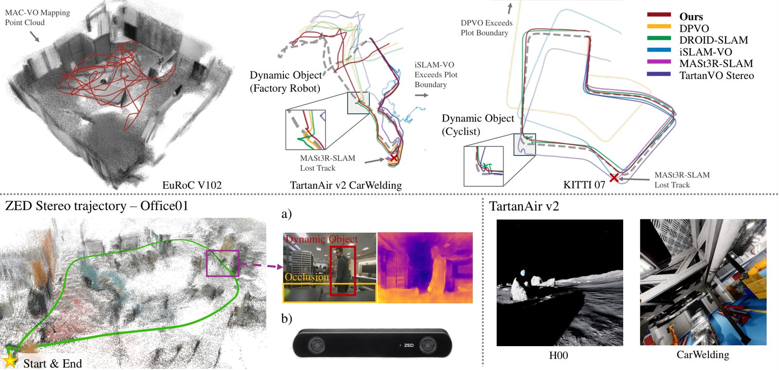
Fig. 6: Top: Trajectories estimated by our model and baselines. We highlight the segments where dynamic objects interrupt the VO. Bottom left: We collect data in the office using our own payload with the ZED-X camera. The data contains multiple dynamic objects and visual occlusions. Bottom right: samples of TartanAir v2 test dataset, which simulates the exotic lunar environment.
图 6:上:我们的模型与基线估计出的轨迹。我们标出了动态物体干扰 VO 的片段。左下:我们用搭载 ZED-X 相机的自制载荷在办公室采集数据,其中包含多个动态物体和视觉遮挡。右下:TartanAir v2 测试集样本,模拟了特征稀少的月球环境。
In addition to quantitative evaluations, we conduct qualitative evaluations of our proposed system across multiple datasets including EuRoC, KITTI, and TartanAir v2, supplemented by manually collected data using a ZED-X stereo camera. MASt3R-SLAM struggles on many trajectories of KITTI and TartanAir, primarily due to incorrect loop closure detections from visual ambiguities. Our model, even without multi-frame optimization, achieves top-tier performance and exhibits fewer glitches than baseline methods. As demonstrated in the Fig. 6, our method produces smoother trajectories and superior pose estimation precision. Fig. 6 a) presents that our model correctly identifies the region occluded by the mounted platform and dynamic objects in the scene and assigns a high uncertainty score to these regions.
除了定量评测,我们还在 EuRoC、KITTI 和 TartanAir v2 等多个数据集上做了定性评估,并补充了用 ZED-X 双目相机手工采集的数据。MASt3R-SLAM 在 KITTI 和 TartanAir 的许多轨迹上表现不佳,主要是因为视觉歧义造成错误的回环检测。我们的模型即使不做多帧优化,也能达到一流水平,毛刺也比基线更少。如图 6 所示,我们的方法得到更平滑的轨迹和更高的位姿估计精度。图 6 a) 表明,模型能正确识别被搭载平台遮挡的区域以及场景中的动态物体,并为这些区域赋以较高的不确定性分数。
| Dataset | TartanAir v2 Hard | TartanAir v2 Easy | ||
|---|---|---|---|---|
| Module Ablation | ||||
| w/o CovKP & CovOpt | .0743 | .5221 | .0521 | .2799 |
| w/o CovOpt | .0679 | .3776 | .0511 | .2367 |
| w/o CovKP | .0188 | .2347 | .0066 | .0808 |
| Covariance Ablation | ||||
| DiagCov | .0461 | .3023 | .0277 | .1548 |
| Scale Agnostic | .0204 | .2321 | .0086 | .0764 |
| Ours | .0141 | .1429 | .0051 | .0670 |
TABLE IV: Ablation study. Detailed results in Appendix B-C.
| Dataset | TartanAir v2 Hard | TartanAir v2 Easy | ||
|---|---|---|---|---|
| 模块消融 | ||||
| w/o CovKP & CovOpt | .0743 | .5221 | .0521 | .2799 |
| w/o CovOpt | .0679 | .3776 | .0511 | .2367 |
| w/o CovKP | .0188 | .2347 | .0066 | .0808 |
| 协方差消融 | ||||
| DiagCov | .0461 | .3023 | .0277 | .1548 |
| 无尺度 | .0204 | .2321 | .0086 | .0764 |
| 本文方法 | .0141 | .1429 | .0051 | .0670 |
表 IV:消融实验。详细结果见附录 B-C。
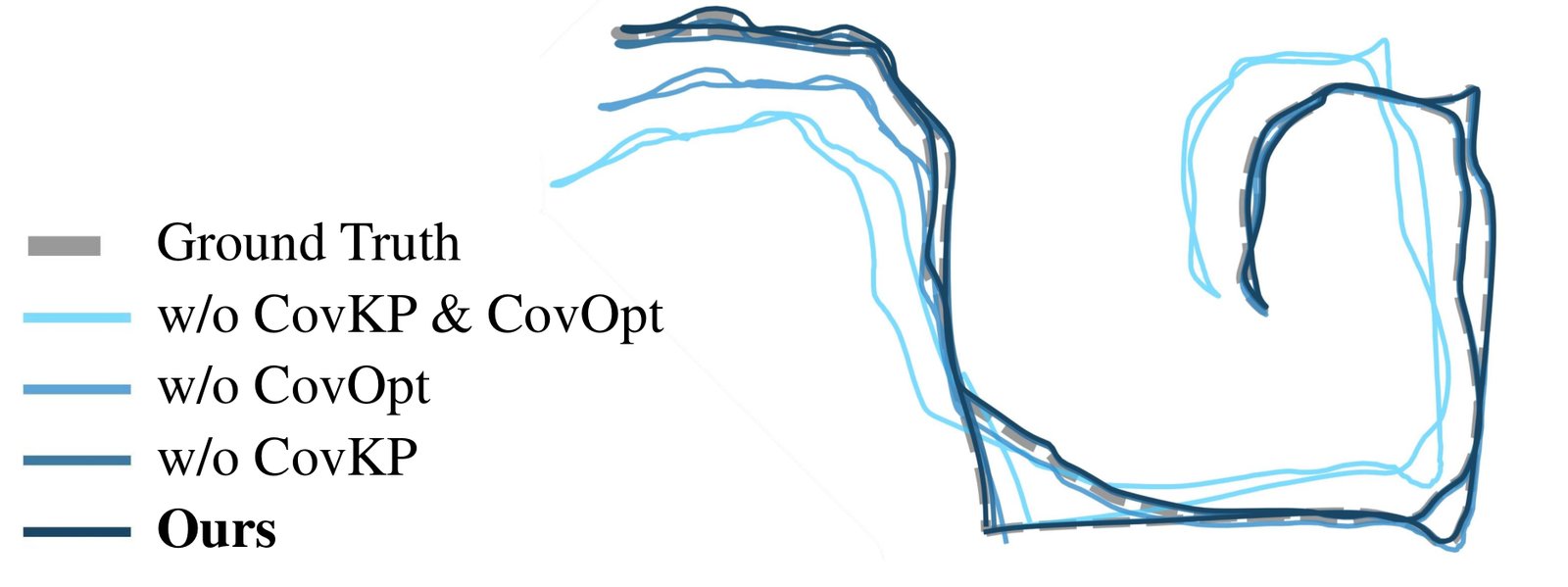
Fig. 7: Results of various ablation setups on the H01 of TartanAirv2.
图 7:TartanAirv2 的 H01 上各种消融设置的结果。
Ablation Study In Table IV, we first perform the ablation study on each module of MAC-VO including (a. w/o CovKP & CovOPT) with random keypoint selector and identity covariance matrix. (b. w/o CovOpt) replace the metrics-aware covariance model with the identity covariance model. (c. w/o CovKP) replace the proposed keypoint selector with a random keypoint selector. To demonstrate the necessity of scale consistency and off-diagonal terms in our covariance model, we run the ablation study with different configurations: (I. DiagCov) remove off-diagonal terms in Eq. 3, (II. Scale-agnostic) normalize the covariance model by the average determinants of covariance matrices of each frame.
消融实验 在表 IV 中,我们首先对 MAC-VO 的各个模块做消融:(a. w/o CovKP & CovOPT)使用随机关键点选择器和单位协方差矩阵。(b. w/o CovOpt)用单位协方差模型替换度量感知协方差模型。(c. w/o CovKP)用随机关键点选择器替换所提出的关键点选择器。为说明协方差模型中尺度一致性和非对角项的必要性,我们还比较了不同配置:(I. DiagCov)去掉式 3 中的非对角项;(II. 无尺度)用每一帧协方差矩阵行列式的平均值对协方差模型做归一化。
| Raw | TRT⋆ | MP† + TRT⋆ | MAC-VO Fast‡ | |
|---|---|---|---|---|
| Modules (ms) | ||||
| Frontend Network | 401.9 | 239.3 | 239.9 | 81.6 |
| Optimization | 53.4 | 57.5 | - | - |
| Motion Model | 5.2 | 5.1 | 5.3 | 5.2 |
| Keypoint Selector | 0.7 | 0.6 | 0.6 | 0.5 |
| Covariance Model | 0.6 | 0.7 | 0.7 | 0.7 |
| Overall (fps) | 2.15 | 3.25 | 3.96 | 10.57 |
| ⋆ TRT: TensorRT framework - https://developer.nvidia.com/tensorrt | ||||
| † MP: multi-processing the PGO in parallel with the matching network. | ||||
| ‡ MAC-VO Fast: utilizes half-precision number (bf16) and light-weight model. |
TABLE V: Time spent on each module of MAC-VO under different optimization with image resolution of .
| Raw | TRT⋆ | MP† + TRT⋆ | MAC-VO Fast‡ | |
|---|---|---|---|---|
| 模块(毫秒) | ||||
| 前端网络 | 401.9 | 239.3 | 239.9 | 81.6 |
| 优化 | 53.4 | 57.5 | - | - |
| 运动模型 | 5.2 | 5.1 | 5.3 | 5.2 |
| 关键点选择器 | 0.7 | 0.6 | 0.6 | 0.5 |
| 协方差模型 | 0.6 | 0.7 | 0.7 | 0.7 |
| 总体(帧/秒) | 2.15 | 3.25 | 3.96 | 10.57 |
| ⋆ TRT:TensorRT 框架,https://developer.nvidia.com/tensorrt | ||||
| † MP:把位姿图优化与匹配网络并行的多进程设置。 | ||||
| ‡ MAC-VO Fast:使用半精度数值(bf16)和更轻量的模型。 |
表 V:图像分辨率为 时,不同优化设置下 MAC-VO 各模块耗时。
IV-C Runtime Analysis
IV-C 运行时间分析
The runtime analysis shown in Table V uses the platform with AMD Ryzen 9 5950X CPU and NVIDIA 3090 Ti GPU. We also introduce a fast mode (MAC-VO Fast) that utilizes half-precision number in the network inference to enhance efficiency. This mode also speeds up the memory decoder network by reducing the number of iterative updates from 12 to 4. The fast mode performs at 10.5 fps (frames per second) with 70% of the performance of the original MAC-VO. More details are included in Appendix C.
表 V 中的运行时间分析使用配备 AMD Ryzen 9 5950X CPU 和 NVIDIA 3090 Ti GPU 的平台。我们还引入了一种快速模式(MAC-VO Fast),在网络推理中使用半精度数值以提高效率。该模式同时把记忆解码器网络的迭代更新次数从 12 次减到 4 次。快速模式达到 10.5 fps(帧每秒),性能约为原始 MAC-VO 的 70%。更多细节见附录 C。
V Conclusion & Discussion
V 结论与讨论
This paper proposes MAC-VO, a learning-based stereo VO method that outperforms most visual odometry and even SLAM algorithms on challenging datasets. In our current work, the model focuses on the two-frame pose optimization. We believe our accuracy will be further benefit from bundle adjustment, multi-frame optimization, and loop closure. Additionally, we plan to apply our metrics-aware covariance model in multi-sensor fusion, such as with IMUs.
本文提出 MAC-VO,这是一种学习型双目 VO 方法,在困难数据集上超过了大多数视觉里程计,甚至超过部分 SLAM 算法。当前工作聚焦于两帧位姿优化。我们相信,引入光束法平差、多帧优化和回环检测后,精度还会进一步提高。此外,我们计划把度量感知协方差模型用于与 IMU 等多传感器的融合。
References
参考文献
[1] R. Mur-Artal, J. M. M. Montiel, and J. D. Tardos, “Orb-slam: a versatile and accurate monocular slam system,” IEEE transactions on robotics , vol. 31, no. 5, pp. 1147–1163, 2015.
[2] W. Wang, Y. Hu, and S. Scherer, “Tartanvo: A generalizable learning-based vo,” 2020.
[3] Z. Teed and J. Deng, “Droid-slam: Deep visual slam for monocular, stereo, and rgb-d cameras,” Advances in neural information processing systems , vol. 34, pp. 16 558–16 569, 2021.
[4] Z. Teed, L. Lipson, and J. Deng, “Deep patch visual odometry,” Advances in Neural Information Processing Systems , vol. 36, 2024.
[5] M. A. Fischler and R. C. Bolles, “Random sample consensus: a paradigm for model fitting with applications to image analysis and automated cartography,” Communications of the ACM , vol. 24, no. 6, pp. 381–395, 1981.
[6] S. Zhao, H. Zhang, P. Wang, L. Nogueira, and S. Scherer, “Super odometry: Imu-centric lidar-visual-inertial estimator for challenging environments,” in 2021 IEEE/RSJ International Conference on Intelligent Robots and Systems (IROS) . IEEE, 2021, pp. 8729–8736.
[7] D. DeTone, T. Malisiewicz, and A. Rabinovich, “Superpoint: Self-supervised interest point detection and description,” in 2018 IEEE/CVF Conference on Computer Vision and Pattern Recognition Workshops (CVPRW) . IEEE, Jun. 2018. [Online]. Available: http://dx.doi.org/10.1109/CVPRW.2018.00060
[8] E. Rublee, V. Rabaud, K. Konolige, and G. Bradski, “Orb: An efficient alternative to sift or surf,” in 2011 International Conference on Computer Vision , 2011, pp. 2564–2571.
[9] D. G. Lowe, “Distinctive image features from scale-invariant keypoints,” Int. J. Comput. Vision , vol. 60, no. 2, p. 91–110, nov 2004. [Online]. Available: https://doi.org/10.1023/B:VISI.0000029664.99615.94
[10] S. Wang, V. Leroy, Y. Cabon, B. Chidlovskii, and J. Revaud, “Dust3r: Geometric 3d vision made easy,” arXiv preprint arXiv:2312.14132 , 2023.
[11] Z. Huang, X. Shi, C. Zhang, Q. Wang, K. C. Cheung, H. Qin, J. Dai, and H. Li, “Flowformer: A transformer architecture for optical flow,” in European conference on computer vision . Springer, 2022, pp. 668–685.
[12] S. Jiang, D. Campbell, Y. Lu, H. Li, and R. Hartley, “Learning to estimate hidden motions with global motion aggregation,” in Proceedings of the IEEE/CVF international conference on computer vision , 2021, pp. 9772–9781.
[13] G. Klein and D. Murray, “Parallel tracking and mapping for small ar workspaces,” in 2007 6th IEEE and ACM international symposium on mixed and augmented reality . IEEE, 2007, pp. 225–234.
[14] R. Wang, M. Schworer, and D. Cremers, “Stereo dso: Large-scale direct sparse visual odometry with stereo cameras,” in Proceedings of the IEEE international conference on computer vision , 2017, pp. 3903–3911.
[15] J. Engel, T. Schöps, and D. Cremers, “Lsd-slam: Large-scale direct monocular slam,” in European conference on computer vision . Springer, 2014, pp. 834–849.
[16] X. Gao, R. Wang, N. Demmel, and D. Cremers, “Ldso: Direct sparse odometry with loop closure,” in International Conference on Intelligent Robots and Systems (IROS) , October 2018.
[17] J. Civera, A. J. Davison, and J. M. M. Montiel, “Inverse depth parametrization for monocular slam,” IEEE Transactions on Robotics , vol. 24, no. 5, pp. 932–945, 2008.
[18] J. M. M. Montiel, J. Civera, and A. J. Davison, “Unified inverse depth parametrization for monocular slam,” in Robotics: Science and Systems , 2006. [Online]. Available: https://api.semanticscholar.org/CorpusID:18457284
[19] T. Qin, P. Li, and S. Shen, “Vins-mono: A robust and versatile monocular visual-inertial state estimator,” IEEE Transactions on Robotics , vol. 34, no. 4, pp. 1004–1020, 2018.
[20] S. Yang and S. Scherer, “Cubeslam: Monocular 3-d object slam,” IEEE Transactions on Robotics , vol. 35, no. 4, pp. 925–938, 2019.
[21] Y. Qiu, C. Wang, W. Wang, M. Henein, and S. Scherer, “Airdos: Dynamic slam benefits from articulated objects,” in 2022 International Conference on Robotics and Automation (ICRA) . IEEE, 2022, pp. 8047–8053.
[22] Z. Teed and J. Deng, “Raft: Recurrent all-pairs field transforms for optical flow,” in Computer Vision–ECCV 2020: 16th European Conference, Glasgow, UK, August 23–28, 2020, Proceedings, Part II 16 . Springer, 2020, pp. 402–419.
[23] C. M. Parameshwara, G. Hari, C. Fermüller, N. J. Sanket, and Y. Aloimonos, “Diffposenet: Direct differentiable camera pose estimation,” in Proceedings of the IEEE/CVF Conference on Computer Vision and Pattern Recognition , 2022, pp. 6845–6854.
[24] P.-E. Sarlin, D. DeTone, T. Malisiewicz, and A. Rabinovich, “Superglue: Learning feature matching with graph neural networks,” in Proceedings of the IEEE/CVF conference on computer vision and pattern recognition , 2020, pp. 4938–4947.
[25] T. Zhou, M. Brown, N. Snavely, and D. G. Lowe, “Unsupervised learning of depth and ego-motion from video,” in Proceedings of the IEEE conference on computer vision and pattern recognition , 2017, pp. 1851–1858.
[26] R. Li, S. Wang, Z. Long, and D. Gu, “Undeepvo: Monocular visual odometry through unsupervised deep learning,” in 2018 IEEE international conference on robotics and automation (ICRA) . IEEE, 2018, pp. 7286–7291.
[27] K. Tateno, F. Tombari, I. Laina, and N. Navab, “Cnn-slam: Real-time dense monocular slam with learned depth prediction,” in Proceedings of the IEEE conference on computer vision and pattern recognition , 2017, pp. 6243–6252.
[28] G. Costante, M. Mancini, P. Valigi, and T. A. Ciarfuglia, “Exploring representation learning with cnns for frame-to-frame ego-motion estimation,” IEEE robotics and automation letters , vol. 1, no. 1, pp. 18–25, 2015.
[29] E. Dexheimer and A. J. Davison, “Learning a depth covariance function,” in 2023 IEEE/CVF Conference on Computer Vision and Pattern Recognition (CVPR) . IEEE, Jun. 2023, p. 13122–13131. [Online]. Available: http://dx.doi.org/10.1109/CVPR52729.2023.01261
[30] X. Nie, D. Shi, R. Li, Z. Liu, and X. Chen, “Uncertainty-aware self-improving framework for depth estimation,” IEEE Robotics and Automation Letters , vol. 7, no. 1, pp. 41–48, 2022.
[31] A. S. Wannenwetsch, M. Keuper, and S. Roth, “Probflow: Joint optical flow and uncertainty estimation,” in Proceedings of the IEEE International Conference on Computer Vision (ICCV) , Oct 2017.
[32] N. Yang, L. v. Stumberg, R. Wang, and D. Cremers, “D3vo: Deep depth, deep pose and deep uncertainty for monocular visual odometry,” in Proceedings of the IEEE/CVF conference on computer vision and pattern recognition , 2020, pp. 1281–1292.
[33] T. Fu, S. Su, Y. Lu, and C. Wang, “islam: Imperative slam,” IEEE Robotics and Automation Letters , 2024.
[34] A. Ranjan, V. Jampani, L. Balles, K. Kim, D. Sun, J. Wulff, and M. J. Black, “Competitive collaboration: Joint unsupervised learning of depth, camera motion, optical flow and motion segmentation,” in Proceedings of the IEEE/CVF conference on computer vision and pattern recognition , 2019, pp. 12 240–12 249.
[35] P.-E. Sarlin, A. Unagar, M. Larsson, H. Germain, C. Toft, V. Larsson, M. Pollefeys, V. Lepetit, L. Hammarstrand, F. Kahl, and T. Sattler, “Back to the feature: Learning robust camera localization from pixels to pose,” in 2021 IEEE/CVF Conference on Computer Vision and Pattern Recognition (CVPR) . IEEE, Jun. 2021. [Online]. Available: http://dx.doi.org/10.1109/CVPR46437.2021.00326
[36] G. Costante and M. Mancini, “Uncertainty estimation for data-driven visual odometry,” IEEE Transactions on Robotics , vol. 36, no. 6, pp. 1738–1757, 2020.
[37] D. Muhle, L. Koestler, K. Jatavallabhula, and D. Cremers, “Learning correspondence uncertainty via differentiable nonlinear least squares,” in Proceedings of the IEEE/CVF Conference on Computer Vision and Pattern Recognition , 2023, pp. 13 102–13 112.
[38] N. Kaygusuz, O. Mendez, and R. Bowden, “Mdn-vo: Estimating visual odometry with confidence,” in 2021 IEEE/RSJ International Conference on Intelligent Robots and Systems (IROS) . IEEE, Sep. 2021. [Online]. Available: http://dx.doi.org/10.1109/IROS51168.2021.9636827
[39] S. Rabiee and J. Biswas, “Iv-slam: Introspective vision for simultaneous localization and mapping,” 2020.
[40] R. Murai, E. Dexheimer, and A. J. Davison, “Mast3r-slam: Real-time dense slam with 3d reconstruction priors,” arXiv preprint arXiv:2412.12392 , 2024.
[41] P. Lindenberger, P.-E. Sarlin, V. Larsson, and M. Pollefeys, “Pixel-perfect structure-from-motion with featuremetric refinement,” in 2021 IEEE/CVF International Conference on Computer Vision (ICCV) . IEEE, Oct. 2021. [Online]. Available: http://dx.doi.org/10.1109/ICCV48922.2021.00593
[42] R. L. Russell and C. Reale, “Multivariate uncertainty in deep learning,” IEEE Transactions on Neural Networks and Learning Systems , vol. 33, no. 12, pp. 7937–7943, 2021.
[43] A. N. Angelopoulos and S. Bates, Conformal Prediction: A Gentle Introduction . Now Foundations and Trends, 2023.
[44] Y. Qiu, C. Wang, C. Xu, Y. Chen, X. Zhou, Y. Xia, and S. Scherer, “Airimu: Learning uncertainty propagation for inertial odometry,” 2023.
[45] W. Wang, D. Zhu, X. Wang, Y. Hu, Y. Qiu, C. Wang, Y. Hu, A. Kapoor, and S. Scherer, “Tartanair: A dataset to push the limits of visual slam,” 2020.
[46] C. Wang, D. Gao, K. Xu, J. Geng, Y. Hu, Y. Qiu, B. Li, F. Yang, B. Moon, A. Pandey et al. , “Pypose: A library for robot learning with physics-based optimization,” in IEEE/CVF Conference on Computer Vision and Pattern Recognition (CVPR) , 2023, pp. 22 024–22 034.
[47] Z. Zhan, X. Li, Q. Li, H. He, A. Pandey, H. Xiao, Y. Xu, X. Chen, K. Xu, K. Cao et al. , “Pypose v0. 6: The imperative programming interface for robotics,” IEEE/RSJ International Conference on Intelligent Robots and Systems (IROS) Workshop , 2023.
[48] M. Burri, J. Nikolic, P. Gohl, T. Schneider, J. Rehder, S. Omari, M. W. Achtelik, and R. Siegwart, “The euroc micro aerial vehicle datasets,” The International Journal of Robotics Research , vol. 35, no. 10, pp. 1157–1163, 2016. [Online]. Available: https://doi.org/10.1177/0278364915620033
[49] A. Geiger, P. Lenz, and R. Urtasun, “Are we ready for autonomous driving? the kitti vision benchmark suite,” in Conference on Computer Vision and Pattern Recognition (CVPR) , 2012.
[50] L. A. Goodman, “On the exact variance of products,” Journal of the American Statistical Association , vol. 55, no. 292, pp. 708–713, 1960. [Online]. Available: https://www.tandfonline.com/doi/abs/10.1080/01621459.1960.10483369
Appendix A Covariance Model Formulation
附录 A 协方差模型的表述
A-A Depth Uncertainty From Disparity Uncertainty
A-A 由视差不确定性得到深度不确定性
In this section, we present the formulation for estimating the distribution of depth on a single pixel given the estimated distribution of disparity .
本节给出:在单个像素上,给定视差的估计分布 时,深度 分布的估计表述。
Following the pinhole camera model, the depth is calculated as where the camera baseline is . Since can be zero, the distribution of may be ill-defined. To fix this, we employ the first-order Taylor expansion to approximate and such that .
按照针孔相机模型,深度由 算出,其中相机基线为 。由于 可能为零, 的分布可能不适定。为解决这一点,我们用一阶泰勒展开近似 和 ,使得 。
We assume the variance of disparity for some sufficiently small such that the probability of is negligible. Based on this assumption, we have
我们假定视差方差 ,其中 足够小,使得 的概率可以忽略。基于这一假定,我们有
Similarly, can be expressed as
类似地, 可以写成
Therefore, the approximation of depth uncertainty from disparity uncertainty is expressed as follows:
因此,由视差不确定性近似得到的深度不确定性表述如下:
Monte Carlo simulation indicates that for , the error of the aforementioned approximation is acceptable, as shown in Fig. 8.
蒙特卡洛模拟表明,当 时,上述近似的误差可以接受,如图 8 所示。
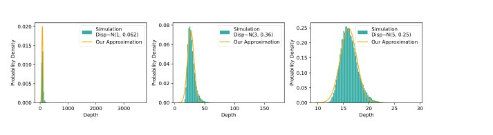
Fig. 8: Result of Monte Carlo simulation on depth distribution. Despite the skewness in the simulated distribution, our approximation matches the simulation. As error rate increases and average disparity approaches (from right to left), the depth distribution becomes more skewed and the quality of approximation decreases.
图 8:深度分布的蒙特卡洛模拟结果。尽管模拟分布存在偏斜,我们的近似仍与模拟相符。随着误差率 增大、平均视差 接近 (从右到左),深度分布更偏斜,近似质量也会下降。
A-B Uncertainty Correction After Keypoint Matching
A-B 关键点匹配后的不确定性校正
Let be the -th keypoint on the camera plane at time . Given the estimated optical flow at , the matched keypoint at time is defined as . Since follows the gaussian distribution , is a random variable following distribution of .
设 为时刻 相机平面上的第 个关键点。给定该点处估计的光流 ,时刻 的匹配关键点定义为 。由于 服从高斯分布 , 是服从 的随机变量。
Let be a 2D Gaussian filter with covariance matrix , the probability for matched keypoint on some pixel is then expressed as . Let denote the estimated depth at pixel , then the average depth for pixel weighted by is expressed as
设 是协方差矩阵为 的二维高斯滤波器,则匹配关键点落在某个像素 上的概率可写成 。设 表示像素 处的估计深度,则像素 按 加权的平均深度写为
and the estimated variance of depth of is calculated as weighted variance
而 的估计深度方差按加权方差计算
We could also model the depth of the matched point using a mixture of Gaussian distributions, but experiments show that this offers only a minimal performance improvement. Therefore, we use the straightforward weighted variance method to estimate depth uncertainty.
我们也可以用高斯混合分布来建模匹配点的深度,但实验表明这样做只能带来很小的性能提升。因此,我们用直接的加权方差方法来估计深度不确定性。
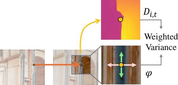
Fig. 9: Estimate depth variance of the matched point under the presence of matching uncertainty
图 9:在存在匹配不确定性时,估计匹配点的深度方差
A-C Projecting 2D Uncertainty to Spatial Covariance
A-C 把二维不确定性投影为空间协方差
Let , , and , we derive the distribution of 3D point under camera coordinate .
设 、 以及 ,我们推导相机坐标系下三维点 的分布。
Recall that the relationship between pixel coordinate , depth and 3D coordinate is depicted as
回顾像素坐标 、深度 与三维坐标 的关系为
Assume , , are independent to each other, we have [50]. Based on this expression of variance, it follows that
假定 、、 彼此独立,则有 [50]。据此方差表达式,可以得到
Under the assumption that are independent to each other, we derive the covariance between , and as:
在 彼此独立的假定下,我们把 、 和 之间的协方差推导为:
and
以及
Fig. 10 visualize the distribution of keypoints in 3D space via Monte Carlo and the 90% confidence interval of estimated distribution, confirming the necessity of off-diagonal terms.
图 10 用蒙特卡洛方法可视化了关键点在三维空间中的分布,以及估计分布的 90% 置信区间,从而证实非对角项是必要的。
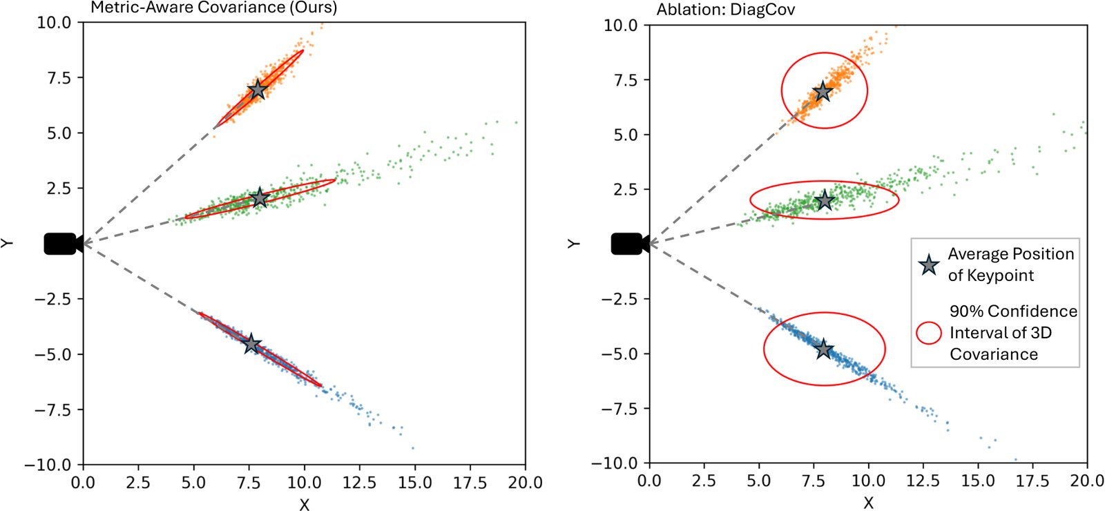
Fig. 10: Comparison of proposed 3D covariance (left) and the diagonal covariance matrix (right, DiagCov in ablation study). Our method captures the uncertainty of keypoints significantly better than the diagonal covariance matrix.
图 10:所提出的三维协方差(左)与对角协方差矩阵(右,即消融实验中的 DiagCov)的比较。我们的方法对关键点不确定性的刻画明显优于对角协方差矩阵。
Appendix B Additional Results
附录 B 补充结果
B-A Remaining Results on EuRoC, TartanAirv2, and KITTI
B-A EuRoC、TartanAirv2 和 KITTI 上的其余结果
See Table VI, Table VII, and Table VIII for data.
数据见表 VI、表 VII 和表 VIII。
| Trajectory | MH02 | MH04 | V101 | V103 | V202 | |||||
|---|---|---|---|---|---|---|---|---|---|---|
| SLAM | ||||||||||
| ORB-SLAM 3 | 0.0036 | 0.0495 | 0.0061 | 0.0501 | 0.0049 | 0.0888 | 0.0137 | 0.2669 | 0.0090 | 0.1528 |
| DROID-SLAM⋆ | 0.0012 | 0.0169 | 0.0031 | 0.0224 | 0.0024 | 0.0314 | 0.0036 | 0.0642 | 0.0017 | 0.0399 |
| MASt3R-SLAM*⋆* | 0.0138 | 0.5493 | 0.0274 | 0.8890 | 0.0130 | 0.5808 | 0.0383 | 1.3178 | 0.0334 | 0.6818 |
| VO | ||||||||||
| TartanVO*⋆* | 0.0172 | 0.0621 | 0.0213 | 0.0681 | 0.0124 | 0.0756 | 0.0263 | 0.1552 | 0.0171 | 0.1251 |
| TartanVO | 0.0289 | 0.5037 | 0.0501 | 0.5400 | 0.0224 | 0.5322 | 0.0351 | 1.3127 | 0.0361 | 1.1607 |
| iSLAM-VO | 0.0041 | 0.0620 | 0.0082 | 0.0682 | 0.0041 | 0.0756 | 0.0088 | 0.1554 | 0.0078 | 0.1252 |
| DPVO*⋆* | 0.0014 | 0.0212 | 0.0029 | 0.0264 | 0.0026 | 0.0405 | 0.0033 | 0.0662 | 0.0022 | 0.0493 |
| Ours | 0.0013 | 0.0199 | 0.0028 | 0.0273 | 0.0024 | 0.0304 | 0.0032 | 0.058 | 0.0018 | 0.0406 |
| Monocular method. Stereo method. ⋆ Scale-aligned with ground truth. |
TABLE VI: Performance comparison of different methods on the EuRoC Dataset. Only even-ordered trajectory is shown here, see Table I for the remaining results.
| 轨迹 | MH02 | MH04 | V101 | V103 | V202 | |||||
|---|---|---|---|---|---|---|---|---|---|---|
| SLAM | ||||||||||
| ORB-SLAM 3 | 0.0036 | 0.0495 | 0.0061 | 0.0501 | 0.0049 | 0.0888 | 0.0137 | 0.2669 | 0.0090 | 0.1528 |
| DROID-SLAM⋆ | 0.0012 | 0.0169 | 0.0031 | 0.0224 | 0.0024 | 0.0314 | 0.0036 | 0.0642 | 0.0017 | 0.0399 |
| MASt3R-SLAM*⋆* | 0.0138 | 0.5493 | 0.0274 | 0.8890 | 0.0130 | 0.5808 | 0.0383 | 1.3178 | 0.0334 | 0.6818 |
| VO | ||||||||||
| TartanVO*⋆* | 0.0172 | 0.0621 | 0.0213 | 0.0681 | 0.0124 | 0.0756 | 0.0263 | 0.1552 | 0.0171 | 0.1251 |
| TartanVO | 0.0289 | 0.5037 | 0.0501 | 0.5400 | 0.0224 | 0.5322 | 0.0351 | 1.3127 | 0.0361 | 1.1607 |
| iSLAM-VO | 0.0041 | 0.0620 | 0.0082 | 0.0682 | 0.0041 | 0.0756 | 0.0088 | 0.1554 | 0.0078 | 0.1252 |
| DPVO*⋆* | 0.0014 | 0.0212 | 0.0029 | 0.0264 | 0.0026 | 0.0405 | 0.0033 | 0.0662 | 0.0022 | 0.0493 |
| 本文方法 | 0.0013 | 0.0199 | 0.0028 | 0.0273 | 0.0024 | 0.0304 | 0.0032 | 0.058 | 0.0018 | 0.0406 |
| 单目方法。 双目方法。 ⋆ 与真值做尺度对齐。 |
表 VI:各方法在 EuRoC 数据集上的性能比较。这里只给出偶数序号轨迹,其余结果见表 I。
| Trajectory | E00 | E01 | E02 | E03 | E04 | E05 | E06 | Avg. | ||||||||
|---|---|---|---|---|---|---|---|---|---|---|---|---|---|---|---|---|
| SLAM | ||||||||||||||||
| ORB-SLAM3 | - | - | .1019 | 2.349 | - | - | - | - | - | - | - | - | - | - | .1019 | 2.349 |
| MASt3R-SLAM*⋆* | .3268 | 2.892 | .3124 | 2.921 | - | - | - | - | .1872 | 2.948 | - | - | .2018 | 3.033 | .2570 | .2948 |
| DROID-SLAM⋆ | .0077 | .0144 | .0025 | .0199 | .0063 | .0409 | .0049 | .0251 | .0009 | .0147 | .0031 | .0463 | .0016 | .0235 | .0039 | .0264 |
| VO | ||||||||||||||||
| TartanVO*⋆* | .0532 | .3237 | .0937 | .4750 | .1066 | .6048 | .0756 | .2230 | .1114 | .4032 | .0862 | .3185 | .1373 | .6620 | .0949 | .4300 |
| TartanVO | .0505 | .1334 | .0322 | .2078 | .0237 | .1105 | .0303 | .1417 | .0173 | .1681 | .0279 | .3828 | .0218 | .2329 | .0291 | .1967 |
| iSLAM-VO | .0656 | .2873 | .0456 | .3853 | .0359 | .2234 | .0508 | .2635 | .0268 | .3201 | .0464 | .6624 | .0362 | .4606 | .0439 | .3718 |
| DPVO*⋆* | .0113 | .0187 | .0047 | .0249 | .0099 | .0475 | .0603 | .2064 | .0044 | .0177 | .0511 | .0665 | .0189 | .1543 | .0229 | .0766 |
| Ours | .0026 | .0351 | .0124 | .1183 | .0031 | .0684 | .0054 | .0383 | .0050 | .0413 | .0018 | .0247 | .0054 | .1427 | .0051 | .0670 |
| Monocular method. Stereo method. ⋆ Scale-aligned with ground truth. |
TABLE VII: Performance comparison on the TartanAir v2 Easy Dataset.
| 轨迹 | E00 | E01 | E02 | E03 | E04 | E05 | E06 | Avg. | ||||||||
|---|---|---|---|---|---|---|---|---|---|---|---|---|---|---|---|---|
| SLAM | ||||||||||||||||
| ORB-SLAM3 | - | - | .1019 | 2.349 | - | - | - | - | - | - | - | - | - | - | .1019 | 2.349 |
| MASt3R-SLAM*⋆* | .3268 | 2.892 | .3124 | 2.921 | - | - | - | - | .1872 | 2.948 | - | - | .2018 | 3.033 | .2570 | .2948 |
| DROID-SLAM⋆ | .0077 | .0144 | .0025 | .0199 | .0063 | .0409 | .0049 | .0251 | .0009 | .0147 | .0031 | .0463 | .0016 | .0235 | .0039 | .0264 |
| VO | ||||||||||||||||
| TartanVO*⋆* | .0532 | .3237 | .0937 | .4750 | .1066 | .6048 | .0756 | .2230 | .1114 | .4032 | .0862 | .3185 | .1373 | .6620 | .0949 | .4300 |
| TartanVO | .0505 | .1334 | .0322 | .2078 | .0237 | .1105 | .0303 | .1417 | .0173 | .1681 | .0279 | .3828 | .0218 | .2329 | .0291 | .1967 |
| iSLAM-VO | .0656 | .2873 | .0456 | .3853 | .0359 | .2234 | .0508 | .2635 | .0268 | .3201 | .0464 | .6624 | .0362 | .4606 | .0439 | .3718 |
| DPVO*⋆* | .0113 | .0187 | .0047 | .0249 | .0099 | .0475 | .0603 | .2064 | .0044 | .0177 | .0511 | .0665 | .0189 | .1543 | .0229 | .0766 |
| 本文方法 | .0026 | .0351 | .0124 | .1183 | .0031 | .0684 | .0054 | .0383 | .0050 | .0413 | .0018 | .0247 | .0054 | .1427 | .0051 | .0670 |
| 单目方法。 双目方法。 ⋆ 与真值做尺度对齐。 |
表 VII:TartanAir v2 Easy 数据集上的性能比较。
| Trajectory | 01 | 03 | 05 | 07 | 09 | |||||
|---|---|---|---|---|---|---|---|---|---|---|
| SLAM | ||||||||||
| ORB-SLAM 3 | 0.0416 | 0.0355 | 0.027 | 0.0425 | 0.0161 | 0.0416 | 0.0155 | 0.0385 | 0.0208 | 0.0444 |
| DROID-SLAM⋆ | 0.7112 | 0.0406 | 0.0182 | 0.0385 | 0.0153 | 0.0353 | 0.0746 | 0.0734 | 0.0214 | 0.0378 |
| MASt3R-SLAM*⋆* | 1.9316 | 0.3442 | 0.5313 | 0.2917 | - | - | 0.3735 | 0.3913 | 0.8414 | 0.5479 |
| VO | ||||||||||
| TartanVO*⋆* | 0.6834 | 0.0895 | 0.1234 | 0.0682 | 0.1821 | 0.0761 | 0.2005 | 0.0847 | 0.1704 | 0.1069 |
| TartanVO | 1.1408 | 0.2455 | 0.0477 | 0.0953 | 0.0637 | 0.0821 | 0.0700 | 0.0931 | 0.0990 | 0.1077 |
| iSLAM-VO | 0.2978 | 0.0896 | 0.0507 | 0.0681 | 0.0504 | 0.0758 | 0.0593 | 0.0842 | 0.0660 | 0.1064 |
| DPVO*⋆* | 0.0942 | 0.0247 | 0.0302 | 0.0330 | 0.2221 | 0.0319 | 0.1064 | 0.0311 | 0.1723 | 0.0336 |
| Ours | 0.2663 | 0.1670 | 0.0187 | 0.0504 | 0.0142 | 0.0466 | 0.0194 | 0.0507 | 0.0182 | 0.0567 |
| Monocular method. Stereo method. ⋆ Scale-aligned with ground truth. |
TABLE VIII: Performance comparison of different methods on the KITTI Dataset. Only odd-numbered trajectory is shown here, see Table III for the remaining results.
| 轨迹 | 01 | 03 | 05 | 07 | 09 | |||||
|---|---|---|---|---|---|---|---|---|---|---|
| SLAM | ||||||||||
| ORB-SLAM 3 | 0.0416 | 0.0355 | 0.027 | 0.0425 | 0.0161 | 0.0416 | 0.0155 | 0.0385 | 0.0208 | 0.0444 |
| DROID-SLAM⋆ | 0.7112 | 0.0406 | 0.0182 | 0.0385 | 0.0153 | 0.0353 | 0.0746 | 0.0734 | 0.0214 | 0.0378 |
| MASt3R-SLAM*⋆* | 1.9316 | 0.3442 | 0.5313 | 0.2917 | - | - | 0.3735 | 0.3913 | 0.8414 | 0.5479 |
| VO | ||||||||||
| TartanVO*⋆* | 0.6834 | 0.0895 | 0.1234 | 0.0682 | 0.1821 | 0.0761 | 0.2005 | 0.0847 | 0.1704 | 0.1069 |
| TartanVO | 1.1408 | 0.2455 | 0.0477 | 0.0953 | 0.0637 | 0.0821 | 0.0700 | 0.0931 | 0.0990 | 0.1077 |
| iSLAM-VO | 0.2978 | 0.0896 | 0.0507 | 0.0681 | 0.0504 | 0.0758 | 0.0593 | 0.0842 | 0.0660 | 0.1064 |
| DPVO*⋆* | 0.0942 | 0.0247 | 0.0302 | 0.0330 | 0.2221 | 0.0319 | 0.1064 | 0.0311 | 0.1723 | 0.0336 |
| 本文方法 | 0.2663 | 0.1670 | 0.0187 | 0.0504 | 0.0142 | 0.0466 | 0.0194 | 0.0507 | 0.0182 | 0.0567 |
| 单目方法。 双目方法。 ⋆ 与真值做尺度对齐。 |
表 VIII:各方法在 KITTI 数据集上的性能比较。这里只给出奇数编号轨迹,其余结果见表 III。
B-B Robustness Analysis
B-B 稳健性分析
See Table IX for data.
数据见表 IX。
| Model | DROID-SLAM | iSLAM-VO | TartanVO*⋆†* | TartanVO | DPVO*⋆†* | Ours |
|---|---|---|---|---|---|---|
| Avg. | 0.072 | 0.383 | 0.169 | 0.107 | 0.318 | 0.045 |
| Avg. | 0.418 | 2.925 | 2.748 | 0.991 | 2.099 | 0.475 |
| ⋆ The estimated sequence is scale-aligned with ground truth. | ||||||
| † Monocular method. |
TABLE IX: Robustness of systems on TartanAir v2 Hard test dataset demonstrate by the average variance of relative translation and rotation error.
| Model | DROID-SLAM | iSLAM-VO | TartanVO*⋆†* | TartanVO | DPVO*⋆†* | 本文方法 |
|---|---|---|---|---|---|---|
| Avg. | 0.072 | 0.383 | 0.169 | 0.107 | 0.318 | 0.045 |
| Avg. | 0.418 | 2.925 | 2.748 | 0.991 | 2.099 | 0.475 |
| ⋆ 估计序列与真值做了尺度对齐。 | ||||||
| † 单目方法。 |
表 IX:各系统在 TartanAir v2 Hard 测试集上的稳健性,用相对平移误差和旋转误差的平均方差表示。
B-C Additional Ablation Study
B-C 补充消融实验
See Table X and Table XI for data.
数据见表 X 和表 XI。
| Relative Translation Error () | |||||||
|---|---|---|---|---|---|---|---|
| Trajectory | H00 | H01 | H02 | H03 | H04 | H05 | H06 |
| System Modules | |||||||
| w/o CovKP & CovOpt | 0.136 | 0.037 | 0.058 | 0.098 | 0.027 | 0.071 | 0.092 |
| w/o CovOpt | 0.171 | 0.033 | 0.061 | 0.106 | 0.023 | 0.034 | 0.048 |
| w/o CovKP | 0.025 | 0.005 | 0.015 | 0.025 | 0.005 | 0.029 | 0.028 |
| Covariance Model | |||||||
| DiagCov | 0.128 | 0.016 | 0.038 | 0.066 | 0.014 | 0.023 | 0.038 |
| Scale Agnostic | 0.041 | 0.004 | 0.018 | 0.027 | 0.005 | 0.021 | 0.027 |
| Ours | 0.008 | 0.034 | 0.005 | 0.015 | 0.009 | 0.005 | 0.020 |
| Relative Rotation Error () | |||||||
|---|---|---|---|---|---|---|---|
| Trajectory | H00 | H01 | H02 | H03 | H04 | H05 | H06 |
| System Modules | |||||||
| w/o CovKP & CovOpt | 0.380 | 0.277 | 0.206 | 0.456 | 0.248 | 0.926 | 1.160 |
| w/o CovOpt | 0.350 | 0.244 | 0.248 | 0.507 | 0.176 | 0.449 | 0.669 |
| w/o CovKP | 0.099 | 0.042 | 0.076 | 0.247 | 0.059 | 0.629 | 0.491 |
| Covariance Model | |||||||
| DiagCov | 0.333 | 0.126 | 0.192 | 0.404 | 0.137 | 0.379 | 0.544 |
| Scale Agnostic | 0.173 | 0.042 | 0.098 | 0.253 | 0.060 | 0.500 | 0.498 |
| Ours | 0.102 | 0.145 | 0.063 | 0.078 | 0.141 | 0.055 | 0.465 |
TABLE X: Performance comparison of different ablation setups on the TartanAir v2 Hard Dataset.
| 相对平移误差() | |||||||
|---|---|---|---|---|---|---|---|
| 轨迹 | H00 | H01 | H02 | H03 | H04 | H05 | H06 |
| 系统模块 | |||||||
| w/o CovKP & CovOpt | 0.136 | 0.037 | 0.058 | 0.098 | 0.027 | 0.071 | 0.092 |
| w/o CovOpt | 0.171 | 0.033 | 0.061 | 0.106 | 0.023 | 0.034 | 0.048 |
| w/o CovKP | 0.025 | 0.005 | 0.015 | 0.025 | 0.005 | 0.029 | 0.028 |
| 协方差模型 | |||||||
| DiagCov | 0.128 | 0.016 | 0.038 | 0.066 | 0.014 | 0.023 | 0.038 |
| 无尺度 | 0.041 | 0.004 | 0.018 | 0.027 | 0.005 | 0.021 | 0.027 |
| 本文方法 | 0.008 | 0.034 | 0.005 | 0.015 | 0.009 | 0.005 | 0.020 |
| 相对旋转误差() | |||||||
|---|---|---|---|---|---|---|---|
| 轨迹 | H00 | H01 | H02 | H03 | H04 | H05 | H06 |
| 系统模块 | |||||||
| w/o CovKP & CovOpt | 0.380 | 0.277 | 0.206 | 0.456 | 0.248 | 0.926 | 1.160 |
| w/o CovOpt | 0.350 | 0.244 | 0.248 | 0.507 | 0.176 | 0.449 | 0.669 |
| w/o CovKP | 0.099 | 0.042 | 0.076 | 0.247 | 0.059 | 0.629 | 0.491 |
| 协方差模型 | |||||||
| DiagCov | 0.333 | 0.126 | 0.192 | 0.404 | 0.137 | 0.379 | 0.544 |
| 无尺度 | 0.173 | 0.042 | 0.098 | 0.253 | 0.060 | 0.500 | 0.498 |
| 本文方法 | 0.102 | 0.145 | 0.063 | 0.078 | 0.141 | 0.055 | 0.465 |
表 X:TartanAir v2 Hard 数据集上不同消融设置的性能比较。
| Relative Translation Error () | |||||||
|---|---|---|---|---|---|---|---|
| Trajectory | E00 | E01 | E02 | E03 | E04 | E05 | E06 |
| System Modules | |||||||
| w/o CovKP & CovOpt | 0.116 | 0.049 | 0.045 | 0.058 | 0.018 | 0.035 | 0.044 |
| w/o CovOpt | 0.124 | 0.052 | 0.048 | 0.070 | 0.016 | 0.020 | 0.027 |
| w/o CovKP | 0.010 | 0.003 | 0.006 | 0.008 | 0.002 | 0.009 | 0.009 |
| Covariance Model | |||||||
| DiagCov | 0.069 | 0.025 | 0.025 | 0.037 | 0.009 | 0.012 | 0.017 |
| Scale Agnostic | 0.026 | 0.004 | 0.006 | 0.009 | 0.002 | 0.005 | 0.008 |
| Ours | 0.003 | 0.012 | 0.003 | 0.005 | 0.005 | 0.002 | 0.005 |
| Relative Rotation Error () | |||||||
|---|---|---|---|---|---|---|---|
| Trajectory | E00 | E01 | E02 | E03 | E04 | E05 | E06 |
| System Modules | |||||||
| w/o CovKP & CovOpt | 0.238 | 0.249 | 0.151 | 0.204 | 0.152 | 0.492 | 0.473 |
| w/o CovOpt | 0.219 | 0.254 | 0.187 | 0.275 | 0.132 | 0.278 | 0.313 |
| w/o CovKP | 0.048 | 0.031 | 0.039 | 0.058 | 0.025 | 0.189 | 0.174 |
| Covariance Model | |||||||
| DiagCov | 0.189 | 0.127 | 0.106 | 0.167 | 0.085 | 0.179 | 0.210 |
| Scale Agnostic | 0.073 | 0.033 | 0.027 | 0.067 | 0.029 | 0.148 | 0.136 |
| Ours | 0.035 | 0.118 | 0.068 | 0.038 | 0.041 | 0.025 | 0.143 |
TABLE XI: Performance comparison of different ablation setups on the TartanAir v2 Easy Dataset.
| 相对平移误差() | |||||||
|---|---|---|---|---|---|---|---|
| 轨迹 | E00 | E01 | E02 | E03 | E04 | E05 | E06 |
| 系统模块 | |||||||
| w/o CovKP & CovOpt | 0.116 | 0.049 | 0.045 | 0.058 | 0.018 | 0.035 | 0.044 |
| w/o CovOpt | 0.124 | 0.052 | 0.048 | 0.070 | 0.016 | 0.020 | 0.027 |
| w/o CovKP | 0.010 | 0.003 | 0.006 | 0.008 | 0.002 | 0.009 | 0.009 |
| 协方差模型 | |||||||
| DiagCov | 0.069 | 0.025 | 0.025 | 0.037 | 0.009 | 0.012 | 0.017 |
| 无尺度 | 0.026 | 0.004 | 0.006 | 0.009 | 0.002 | 0.005 | 0.008 |
| 本文方法 | 0.003 | 0.012 | 0.003 | 0.005 | 0.005 | 0.002 | 0.005 |
| 相对旋转误差() | |||||||
|---|---|---|---|---|---|---|---|
| 轨迹 | E00 | E01 | E02 | E03 | E04 | E05 | E06 |
| 系统模块 | |||||||
| w/o CovKP & CovOpt | 0.238 | 0.249 | 0.151 | 0.204 | 0.152 | 0.492 | 0.473 |
| w/o CovOpt | 0.219 | 0.254 | 0.187 | 0.275 | 0.132 | 0.278 | 0.313 |
| w/o CovKP | 0.048 | 0.031 | 0.039 | 0.058 | 0.025 | 0.189 | 0.174 |
| 协方差模型 | |||||||
| DiagCov | 0.189 | 0.127 | 0.106 | 0.167 | 0.085 | 0.179 | 0.210 |
| 无尺度 | 0.073 | 0.033 | 0.027 | 0.067 | 0.029 | 0.148 | 0.136 |
| 本文方法 | 0.035 | 0.118 | 0.068 | 0.038 | 0.041 | 0.025 | 0.143 |
表 XI:TartanAir v2 Easy 数据集上不同消融设置的性能比较。
B-D Datasets and Implementation
B-D 数据集与实现
TartanAir dataset
The Tartanair dataset is a large-scale synthetic dataset encompassing highly diverse scenes, including various complex and challenging environments. Following the TartanAir data generation method, we created new, more diverse and challenging trajectories. From these, we selected that feature fast camera movements, low-light indoor environments, and simulated lunar surfaces lacking visual features. The images in the new dataset have a resolution of . When testing iSLAM-VO and TartanVO, we resized the input images to to match the input requirements of the optical flow network. Due to the substantial GPU memory required by DROID-SLAM for global bundle adjustment optimization when processing high-resolution images, we reduced the input image resolution to and manually reclaimed GPU and memory after testing each trajectory to avoid potential memory insufficiency.
TartanAir 数据集
TartanAir 是一个大规模合成数据集,场景高度多样,包含多种复杂而困难的环境。我们沿用 TartanAir 的数据生成方法,制作了更多样、也更困难的新轨迹,并从中选出相机运动很快、室内低光照,以及缺少视觉特征的模拟月面轨迹。新数据集中的图像分辨率为 。测试 iSLAM-VO 和 TartanVO 时,我们把输入图像缩放到 ,以匹配光流网络的输入要求。DROID-SLAM 在处理高分辨率图像时,全局光束法平差会占用大量 GPU 内存,因此我们把输入分辨率降到 ,并在测完每条轨迹后手动回收 GPU 和内存,以免出现内存不足。
KITTI dataset
The KITTI dataset is a well-known and widely used dataset for autonomous driving, containing detailed ground truth labels that make it suitable for evaluating the performance of various VO/SLAM methods. Learning-based methods may experience performance degradation when handling the image sizes in the KITTI dataset, therefore, we cropped the input images to different sizes based on the methods tested. Our model processed images cropped to , while for testing DROID-SLAM, the images were cropped to .
KITTI 数据集
KITTI 是自动驾驶领域广为使用的数据集,带有详细的真值标注,适合评估各类 VO/SLAM 方法。学习方法在处理 KITTI 的图像尺寸时可能出现性能下降,因此我们按所测方法把输入图像裁成不同尺寸。我们的模型处理裁到 的图像;测试 DROID-SLAM 时,图像被裁到 。
EuRoC dataset
The Euroc dataset consists of 11 trajectories collected by a drone and is also a widely used benchmark for VO/SLAM tasks. Some scenes in this dataset contain thousands of image pairs, which imposes computational pressure on DROID-SLAM when performing bundle adjustment. Thus, during testing, we reduced the input image resolution to and read every other frame of image pairs. In post-processing, we completed the entire trajectory by interpolating timestamps.
EuRoC 数据集
EuRoC 数据集包含无人机采集的 11 条轨迹,同样是 VO/SLAM 任务中常用的基准。其中一些场景包含数千对图像,会给 DROID-SLAM 做光束法平差带来计算压力。因此测试时,我们把输入分辨率降到 ,并隔帧读取图像对。后处理中,我们通过插值时间戳补全整条轨迹。
ZED Camera data
The ZED Camera data comprises real-world trajectory data captured using a ZED stereo camera, employed to test the robustness and generality of our model when faced with unseen data not present in the training set.
ZED 相机数据
ZED 相机数据是用 ZED 双目相机采集的真实轨迹,用来测试模型在训练集中未见过的数据上的稳健性和通用性。
B-E Network and Training Details
B-E 网络与训练细节
In the uncertainty-aware matching network, we employ a flow decoder similar to Flowformer to obtain . In each iteration, the flow is updated by . With the shared features, we finetune a new decoder with ConvGRU layers to estimate the uncertainty updates . In each iteration, the matching uncertainty is updated by .
在感知不确定性的匹配网络中,我们采用与 Flowformer 类似的光流解码器来得到 。每次迭代中,光流 按 更新。借助共享特征,我们微调一个带 ConvGRU 层的新解码器来估计不确定性更新 。每次迭代中,匹配不确定性按 更新。
For each pixel , we extract the local cost-map patch from the cost map, and the context feature from the context encoder. We encode the using a transformer FFN. Given the 2D position , we encode it into positional embedding . We aggregate these features using CNN encoder ME to generate local motion features . Utilizing the GMA module, the network’s global motion features are acquired from the current motion features and . Subsequently, the shared motion features is obtained by concatenating the , and , where is the attention of the context features. To estimate the flow update and , we use the ConvGRU
对每个像素 ,我们从代价图中提取局部代价图块 ,并从上下文编码器提取上下文特征 。我们用 Transformer 的 FFN 编码 。给定二维位置 ,我们把它编码成位置嵌入 。我们用 CNN 编码器 ME 聚合这些特征,生成局部运动特征 。借助 GMA 模块,网络的全局运动特征 由当前运动特征 和 得到。随后,共享运动特征 由拼接 、 和 得到,其中 是上下文特征的注意力。为估计光流更新 和 ,我们使用 ConvGRU
We use AdamW optimizer with a learning rate of . The model is trained on A100 GPU consuming 16 GB GPU memory.
我们使用 AdamW 优化器,学习率为 。模型在 A100 GPU 上训练,占用 16 GB 显存。
B-F GPU memory & Parameters
B-F GPU 内存与参数量
As shown in Table XII, we use 4.20GB of GPU memory, which is 6.7 times smaller than DROID-SLAM. This is because we utilize the sparse features for back-end optimization, reducing the requirements for the GPU memory.
如表 XII 所示,我们使用 4.20GB GPU 内存,比 DROID-SLAM 小 6.7 倍。这是因为我们用稀疏特征做后端优化,降低了对 GPU 内存的需求。
| Methods | GPU memory | Parameters |
|---|---|---|
| Ours | 4.20GB | 19.2M |
| TartanVO-stereo | 1.16GB | 47.3M |
| DROID-SLAM | 28.34GB | 4.0M |
| DPVO | 1.51GB | 3.4M |
TABLE XII: The GPU memory consumption and the number of parameters during testing
| 方法 | GPU 内存 | 参数量 |
|---|---|---|
| 本文方法 | 4.20GB | 19.2M |
| TartanVO-stereo | 1.16GB | 47.3M |
| DROID-SLAM | 28.34GB | 4.0M |
| DPVO | 1.51GB | 3.4M |
表 XII:测试时的 GPU 内存占用和参数量
Appendix C Runtime Analysis
附录 C 运行时间分析

Fig. 11: Multiprocessing setup places the optimizer in the background process and parallelizes the CPU-intensive (optimizer) and GPU-intensive (frontend network inference) jobs.
图 11:多进程设置把优化器放到后台进程,从而把偏 CPU 的工作(优化器)和偏 GPU 的工作(前端网络推理)并行起来。
The runtime analysis use the platform with AMD Ryzen 9 5950X CPU and NVIDIA 3090 Ti GPU. To speed up the frontend network, we utilize TensorRT[^1] (TRT), and multi-processing (MP) to accelerate the original network (Raw). In our multiprocessing setup, as shown in Fig. 11, a new CPU process is initiated to run the pose graph optimization in parallel with the front-end network, thereby maximizing GPU utilization.
运行时间分析使用配备 AMD Ryzen 9 5950X CPU 和 NVIDIA 3090 Ti GPU 的平台。为加速前端网络,我们使用 TensorRT[^1](TRT),并用多进程(MP)加速原始网络(Raw)。如图 11 所示,我们的多进程设置会新开一个 CPU 进程,与前端网络并行运行位姿图优化,从而尽量提高 GPU 利用率。
We also introduce a fast mode (MAC-VO Fast) which utilizes half-precision (bfloat16) number in the network inference to enhance computational efficiency. This mode also speeds up the memory decoder network by reducing the number of iterative updates from 12 to 4. The fast mode performs 10.5 fps (frames per second) with 70% of the performance of the original MAC-VO.
我们还引入了一种快速模式(MAC-VO Fast),在网络推理中使用半精度(bfloat16)数值以提高计算效率。该模式同时把记忆解码器网络的迭代更新次数从 12 次减到 4 次。快速模式达到 10.5 fps(帧每秒),性能约为原始 MAC-VO 的 70%。