Effective Approaches to Attention-based Neural Machine Translation

Minh-Thang Luong Hieu Pham Christopher D. Manning Affiliation:  Computer Science Department, Stanford University, Stanford, CA 94305 Email:  {lmthang,hyhieu,manning}@stanford.edu

Abstract

摘要

An attentional mechanism has lately been used to improve neural machine translation (NMT) by selectively focusing on parts of the source sentence during translation. However, there has been little work exploring useful architectures for attention-based NMT. This paper examines two simple and effective classes of attentional mechanism: a global approach which always attends to all source words and a local one that only looks at a subset of source words at a time. We demonstrate the effectiveness of both approaches on the WMT translation tasks between English and German in both directions. With local attention, we achieve a significant gain of 5.0 BLEU points over non-attentional systems that already incorporate known techniques such as dropout. Our ensemble model using different attention architectures yields a new state-of-the-art result in the WMT’15 English to German translation task with 25.9 BLEU points, an improvement of 1.0 BLEU points over the existing best system backed by NMT and an $n$-gram reranker.[^1]

[^1]: All our code and models are publicly available at http://nlp.stanford.edu/projects/nmt.

最近，人们用注意力机制来改进神经机器翻译（NMT）：在翻译时有选择地关注源句的某些部分。不过，对基于注意力的 NMT 有用结构，相关探索还很少。本文考察两类简单而有效的注意力机制：一种全局方法，始终关注所有源词；一种局部方法，每次只看源词的一个子集。我们在 WMT 英德双向翻译任务上展示了两种方法的有效性。采用局部注意力后，相对已经加入 dropout 等已知技术的无注意力系统，我们取得了 5.0 BLEU 的显著提升。把不同注意力结构组成集成模型后，我们在 WMT’15 英译德任务上得到 25.9 BLEU 的新的当时最好结果，比当时由 NMT 外加 $n$ 元重排序支撑的最好系统高出 1.0 BLEU。[^1]

[^1]: 我们的全部代码和模型公开于 http://nlp.stanford.edu/projects/nmt。

1 Introduction

1 引言

Neural Machine Translation (NMT) achieved state-of-the-art performances in large-scale translation tasks such as from English to French [Luong et al. (2015] and English to German [Jean et al. (2015]. NMT is appealing since it requires minimal domain knowledge and is conceptually simple. The model by ?) reads through all the source words until the end-of-sentence symbol $<$eos$>$ is reached. It then starts emitting one target word at a time, as illustrated in Figure 1. NMT is often a large neural network that is trained in an end-to-end fashion and has the ability to generalize well to very long word sequences. This means the model does not have to explicitly store gigantic phrase tables and language models as in the case of standard MT; hence, NMT has a small memory footprint. Lastly, implementing NMT decoders is easy unlike the highly intricate decoders in standard MT [Koehn et al. (2003].

神经机器翻译（NMT）已在英译法 [Luong et al. (2015] 和英译德 [Jean et al. (2015] 等大规模翻译任务上达到当时最好水平。NMT 的吸引力在于：所需的领域知识很少，概念上也简单。Sutskever 等人的模型会读完所有源词，直到遇到句末符号 $<$eos$>$，然后开始一次生成一个目标词，如图 1 所示。NMT 往往是一个端到端训练的大型神经网络，对很长的词序列也有较好的泛化能力。这意味着模型不必像常规机器翻译那样显式存储庞大的短语表和语言模型，因此内存占用更小。最后，实现 NMT 解码器并不困难，而不像常规机器翻译中高度复杂的解码器 [Koehn et al. (2003]。

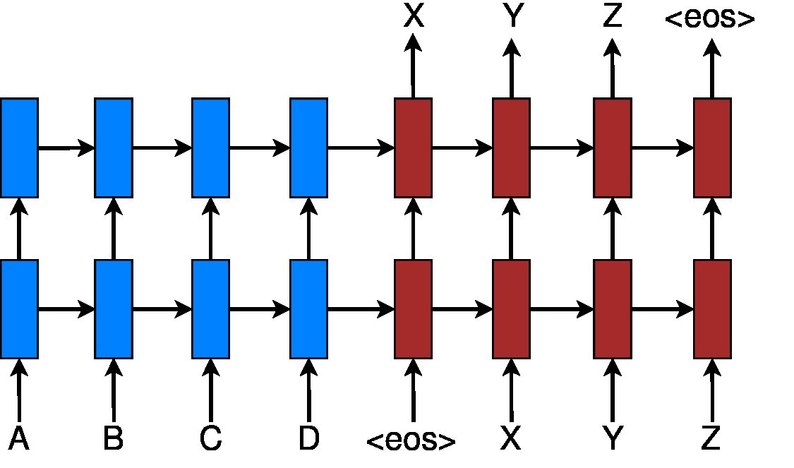
Figure 1: Neural machine translation – a stacking recurrent architecture for translating a source sequence A B C D into a target sequence X Y Z. Here, $<$eos$>$ marks the end of a sentence.

图 1：神经机器翻译——一种堆叠循环结构，把源序列 A B C D 翻译成目标序列 X Y Z。这里的 $<$eos$>$ 标记句子结束。

In parallel, the concept of “attention” has gained popularity recently in training neural networks, allowing models to learn alignments between different modalities, e.g., between image objects and agent actions in the dynamic control problem [Mnih et al. (2014], between speech frames and text in the speech recognition task [jan14], or between visual features of a picture and its text description in the image caption generation task [Xu et al. (2015]. In the context of NMT, ?) has successfully applied such attentional mechanism to jointly translate and align words. To the best of our knowledge, there has not been any other work exploring the use of attention-based architectures for NMT.

与此同时，“注意力”这一概念近来在训练神经网络中流行起来，使模型能够学习不同模态之间的对齐，例如动态控制问题中图像物体与智能体动作之间 [Mnih et al. (2014]、语音识别中语音帧与文本之间 [jan14]，或图像描述生成中图片视觉特征与文字描述之间 [Xu et al. (2015]。在 NMT 的语境里，Bahdanau 等人已经成功地把这种注意力机制用于同时翻译并对齐词。据我们所知，尚未有其他工作探索把基于注意力的结构用于 NMT。

In this work, we design, with simplicity and effectiveness in mind, two novel types of attention-based models: a global approach in which all source words are attended and a local one whereby only a subset of source words are considered at a time. The former approach resembles the model of [Bahdanau et al. (2015] but is simpler architecturally. The latter can be viewed as an interesting blend between the hard and soft attention models proposed in [Xu et al. (2015]: it is computationally less expensive than the global model or the soft attention; at the same time, unlike the hard attention, the local attention is differentiable almost everywhere, making it easier to implement and train.[^2] Besides, we also examine various alignment functions for our attention-based models.

[^2]: There is a recent work by Gregor et al. (2015), which is very similar to our local attention and applied to the image generation task. However, as we detail later, our model is much simpler and can achieve good performance for NMT.

在本工作中，我们以简单和有效为出发点，设计了两类新的基于注意力的模型：一种全局方法，对所有源词施加注意力；一种局部方法，每次只考虑源词的一个子集。前者在思路上接近 [Bahdanau et al. (2015] 的模型，但结构更简单。后者可以看作 [Xu et al. (2015] 中提出的硬注意力与软注意力的一种有趣折中：它的计算代价低于全局模型或软注意力；同时，与硬注意力不同，局部注意力几乎处处可微，因而更容易实现和训练。[^2] 此外，我们还为基于注意力的模型考察了多种对齐函数。

[^2]: 近期有 Gregor 等人（2015）的工作，与我们的局部注意力非常相似，并用于图像生成任务。不过正如后文所述，我们的模型要简单得多，并且在 NMT 上也能取得好的性能。

Experimentally, we demonstrate that both of our approaches are effective in the WMT translation tasks between English and German in both directions. Our attentional models yield a boost of up to 5.0 BLEU over non-attentional systems which already incorporate known techniques such as dropout. For English to German translation, we achieve new state-of-the-art (SOTA) results for both WMT’14 and WMT’15, outperforming previous SOTA systems, backed by NMT models and $n$-gram LM rerankers, by more than 1.0 BLEU. We conduct extensive analysis to evaluate our models in terms of learning, the ability to handle long sentences, choices of attentional architectures, alignment quality, and translation outputs.

实验上，我们表明两种方法在 WMT 英德双向翻译任务中都有效。我们的注意力模型相对已经加入 dropout 等已知技术的无注意力系统，最高可提升 5.0 BLEU。在英译德方向，我们在 WMT’14 和 WMT’15 上都取得了新的当时最好（SOTA）结果，比此前由 NMT 模型加 $n$ 元语言模型重排序支撑的最好系统高出 1.0 BLEU 以上。我们还做了详尽分析，从学习过程、处理长句的能力、注意力结构的选择、对齐质量以及翻译输出等方面评估模型。

2 Neural Machine Translation

2 神经机器翻译

A neural machine translation system is a neural network that directly models the conditional probability $p(y|x)$ of translating a source sentence, $x_{1},\ldots,x_{n}$, to a target sentence, $y_{1},\ldots,y_{m}$.[^3] A basic form of NMT consists of two components: (a) an encoder which computes a representation $s$ for each source sentence and (b) a decoder which generates one target word at a time and hence decomposes the conditional probability as:

[^3]: All sentences are assumed to terminate with a special “end-of-sentence” token $<$eos$>$.

神经机器翻译系统是一个直接建模条件概率 $p(y|x)$ 的神经网络，把源句 $x_{1},\ldots,x_{n}$ 翻译成目标句 $y_{1},\ldots,y_{m}$。[^3] NMT 的基本形式包含两个部分：（a）一个编码器，为每个源句计算表示 $s$；（b）一个解码器，一次生成一个目标词，从而把条件概率分解为：

[^3]: 假定所有句子都以一个特殊的“句末”标记 $<$eos$>$ 结束。

\log p(y|x)=\sum_{j=1}^{m}\nolimits\log p\left(y_{j}|y_{<j},\mbox{\boldmath{$s$}}\right) \tag{1}

A natural choice to model such a decomposition in the decoder is to use a recurrent neural network (RNN) architecture, which most of the recent NMT work such as [Kalchbrenner and Blunsom (2013, Sutskever et al. (2014, Cho et al. (2014, Bahdanau et al. (2015, Luong et al. (2015, Jean et al. (2015] have in common. They, however, differ in terms of which RNN architectures are used for the decoder and how the encoder computes the source sentence representation $s$.

在解码器中对这种分解建模，一个自然的选择是循环神经网络（RNN）结构。近期大多数 NMT 工作，如 [Kalchbrenner and Blunsom (2013, Sutskever et al. (2014, Cho et al. (2014, Bahdanau et al. (2015, Luong et al. (2015, Jean et al. (2015]，都采用了这一结构。不过，它们在解码器使用哪种 RNN 结构、以及编码器如何计算源句表示 $s$ 上有所不同。

?) used an RNN with the standard hidden unit for the decoder and a convolutional neural network for encoding the source sentence representation. On the other hand, both ?) and ?) stacked multiple layers of an RNN with a Long Short-Term Memory (LSTM) hidden unit for both the encoder and the decoder. ?), ?), and ?) all adopted a different version of the RNN with an LSTM-inspired hidden unit, the gated recurrent unit (GRU), for both components.[^4]

[^4]: They all used a single RNN layer except for the latter two works which utilized a bidirectional RNN for the encoder.

Kalchbrenner 与 Blunsom 在解码器中使用带标准隐单元的 RNN，并用卷积神经网络来编码源句表示。另一方面，Sutskever 等人和 Luong 等人在编码器和解码器上都堆叠了多层带长短期记忆（LSTM）隐单元的 RNN。Cho、Bahdanau 和 Jean 则都采用了另一种受 LSTM 启发的 RNN 隐单元，即门控循环单元（GRU），并用于两个组件。[^4]

[^4]: 他们都只用了单层 RNN，只有后两篇工作在编码器中使用了双向 RNN。

In more detail, one can parameterize the probability of decoding each word $y_{j}$ as:

更具体地说，可以把解码每个词 $y_{j}$ 的概率参数化为：

p\left(y_{j}|y_{<j},\mbox{\boldmath{$s$}}\right)=\softmax\left(g\left(\mbox{\boldmath{$h$}}_{j}\right)\right) \tag{2}

with $g$ being the transformation function that outputs a vocabulary-sized vector.[^5] Here, \mbox{\boldmath{h}}_{j} is the RNN hidden unit, abstractly computed as:

[^5]: One can provide $g$ with other inputs such as the currently predicted word $y_{j}$ as in [Bahdanau et al. (2015].

其中 $g$ 是输出一个词表大小向量的变换函数。[^5] 这里，\mbox{\boldmath{h}}_{j} 是 RNN 隐单元，抽象地计算为：

[^5]: 也可以给 $g$ 提供其他输入，例如当前预测词 $y_{j}$，如 [Bahdanau et al. (2015] 中那样。

\mbox{\boldmath{$h$}}_{j}=f(\mbox{\boldmath{$h$}}_{j-1},\mbox{\boldmath{$s$}}), \tag{3}

where $f$ computes the current hidden state given the previous hidden state and can be either a vanilla RNN unit, a GRU, or an LSTM unit. In [Kalchbrenner and Blunsom (2013, Sutskever et al. (2014, Cho et al. (2014, Luong et al. (2015], the source representation $s$ is only used once to initialize the decoder hidden state. On the other hand, in [Bahdanau et al. (2015, Jean et al. (2015] and this work, $s$, in fact, implies a set of source hidden states which are consulted throughout the entire course of the translation process. Such an approach is referred to as an attention mechanism, which we will discuss next.

其中 $f$ 根据前一隐状态计算当前隐状态，可以是普通 RNN 单元、GRU 或 LSTM 单元。在 [Kalchbrenner and Blunsom (2013, Sutskever et al. (2014, Cho et al. (2014, Luong et al. (2015] 中，源表示 $s$ 只被用来初始化解码器隐状态一次。而在 [Bahdanau et al. (2015, Jean et al. (2015] 以及本工作中，$s$ 实际上指一组源端隐状态，在整个翻译过程中都会被查询。这种方法称为注意力机制，我们将在下一节讨论。

In this work, following [Sutskever et al. (2014, Luong et al. (2015], we use the stacking LSTM architecture for our NMT systems, as illustrated in Figure 1. We use the LSTM unit defined in [Zaremba et al. (2015]. Our training objective is formulated as follows:

在本工作中，我们沿用 [Sutskever et al. (2014, Luong et al. (2015]，为 NMT 系统使用堆叠 LSTM 结构，如图 1 所示。我们采用 [Zaremba et al. (2015] 中定义的 LSTM 单元。训练目标表述如下：

$$J_{t}=\sum_{(x,y)\in\mathbb{D}}\nolimits-\log p(y|x) \tag{4}$$

with $\mathbb{D}$ being our parallel training corpus.

其中 $\mathbb{D}$ 是我们的平行训练语料。

3 Attention-based Models

3 基于注意力的模型

Our various attention-based models are classifed into two broad categories, global and local. These classes differ in terms of whether the “attention” is placed on all source positions or on only a few source positions. We illustrate these two model types in Figure 2 and 3 respectively.

我们的各种基于注意力的模型分成两大类：全局和局部。两类的差别在于，“注意力”是放在所有源位置上，还是只放在少数源位置上。我们分别在图 2 和图 3 中展示这两类模型。

Common to these two types of models is the fact that at each time step $t$ in the decoding phase, both approaches first take as input the hidden state \mbox{\boldmath{h}}_{t} at the top layer of a stacking LSTM. The goal is then to derive a context vector \mbox{\boldmath{c}}_{t} that captures relevant source-side information to help predict the current target word $y_{t}$. While these models differ in how the context vector \mbox{\boldmath{c}}_{t} is derived, they share the same subsequent steps.

这两类模型的共同点是：在解码阶段的每个时间步 $t$，两种方法都先把堆叠 LSTM 顶层的隐状态 \mbox{\boldmath{h}}_{t} 作为输入。随后的目标是得到一个上下文向量 \mbox{\boldmath{c}}_{t}，用来捕捉有助于预测当前目标词 $y_{t}$ 的相关源端信息。这些模型在如何得到上下文向量 \mbox{\boldmath{c}}_{t} 上有所不同，但后续步骤是一样的。

Specifically, given the target hidden state \mbox{\boldmath{h}}_{t} and the source-side context vector \mbox{\boldmath{c}}_{t}, we employ a simple concatenation layer to combine the information from both vectors to produce an attentional hidden state as follows:

具体而言，给定目标隐状态 \mbox{\boldmath{h}}_{t} 和源端上下文向量 \mbox{\boldmath{c}}_{t}，我们用一个简单的拼接层把两个向量中的信息结合起来，得到注意力隐状态，如下所示：

\mbox{\boldmath{$\tilde{h}$}}_{t}=\tanh(\mbox{\boldmath{$W_{c}$}}[\mbox{\boldmath{$c$}}_{t};\mbox{\boldmath{$h$}}_{t}]) \tag{5}

The attentional vector \mbox{\boldmath{\tilde{h}}}_{t} is then fed through the softmax layer to produce the predictive distribution formulated as:

然后，把注意力向量 \mbox{\boldmath{\tilde{h}}}_{t} 送入 softmax 层，得到如下形式的预测分布：

p(y_{t}|y_{<t},x)=\softmax(\mbox{\boldmath{$W_{s}$}}\mbox{\boldmath{$\tilde{h}$}}_{t}) \tag{6}

We now detail how each model type computes the source-side context vector \mbox{\boldmath{c}}_{t}.

下面我们详细说明每类模型如何计算源端上下文向量 \mbox{\boldmath{c}}_{t}。

3.1 Global Attention

3.1 全局注意力

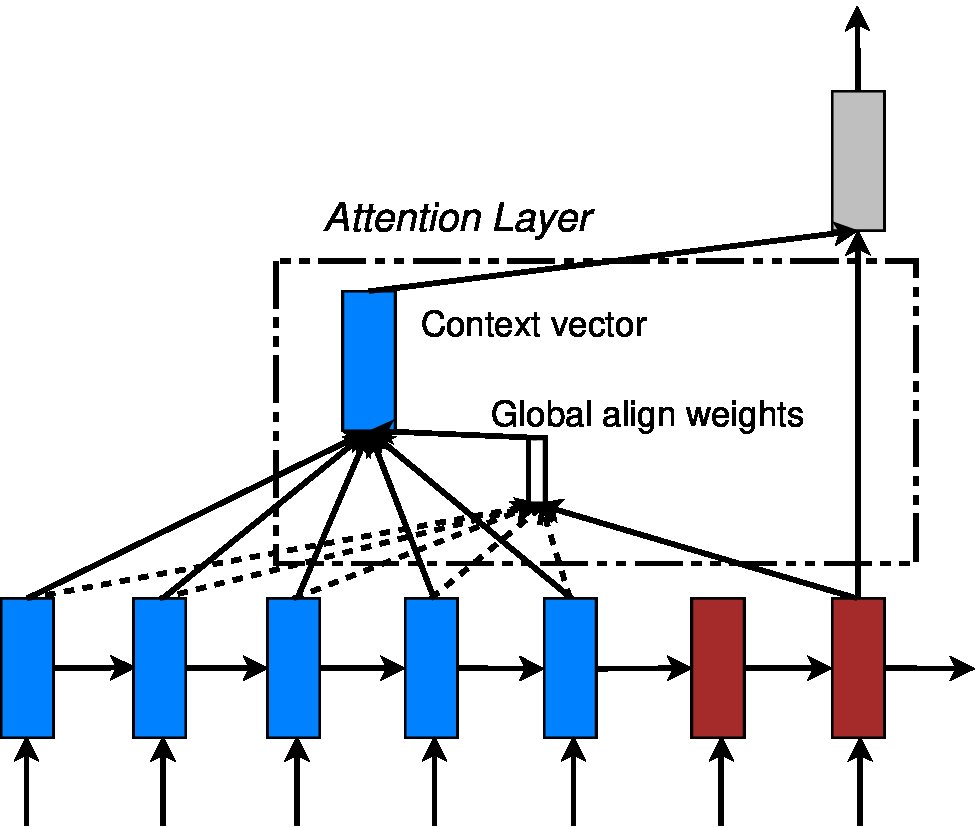
Figure 2: Global attentional model – at each time step $t$, the model infers a variable-length alignment weight vector \mbox{\boldmath{a}}_{t} based on the current target state \mbox{\boldmath{h}}_{t} and all source states \mbox{\boldmath{\bar{h}}}_{s}. A global context vector \mbox{\boldmath{c}}_{t} is then computed as the weighted average, according to \mbox{\boldmath{a}}_{t}, over all the source states.

图 2：全局注意力模型——在每个时间步 $t$，模型根据当前目标状态 \mbox{\boldmath{h}}_{t} 和所有源状态 \mbox{\boldmath{\bar{h}}}_{s}，推断一个可变长度的对齐权重向量 \mbox{\boldmath{a}}_{t}。然后按 \mbox{\boldmath{a}}_{t} 对所有源状态做加权平均，得到全局上下文向量 \mbox{\boldmath{c}}_{t}。

The idea of a global attentional model is to consider all the hidden states of the encoder when deriving the context vector $c_{t}$. In this model type, a variable-length alignment vector \mbox{\boldmath{a}}_{t}, whose size equals the number of time steps on the source side, is derived by comparing the current target hidden state \mbox{\boldmath{h}}_{t} with each source hidden state \mbox{\boldmath{\bar{h}}}_{s}:

全局注意力模型的想法是：在推导上下文向量 $c_{t}$ 时考虑编码器的全部隐状态。在这类模型中，通过把当前目标隐状态 \mbox{\boldmath{h}}_{t} 与每个源隐状态 \mbox{\boldmath{\bar{h}}}_{s} 比较，得到一个可变长度的对齐向量 \mbox{\boldmath{a}}_{t}，其大小等于源端的时间步数：

\displaystyle\mbox{\boldmath{$a$}}_{t}(s) \\ \displaystyle=\alignf(\mbox{\boldmath{$h$}}_{t},\mbox{\boldmath{$\bar{h}$}}_{s}) \\ \displaystyle=\frac{\exp\left(\score(\mbox{\boldmath{$h$}}_{t},\mbox{\boldmath{$\bar{h}$}}_{s})\right)}{\sum_{s^{\prime}}\exp\left(\score(\mbox{\boldmath{$h$}}_{t},\mbox{\boldmath{$\bar{h}$}}_{s^{\prime}})\right)} \tag{7}

Here, $\score$ is referred as a content-based function for which we consider three different alternatives:

这里，$\score$ 称为基于内容的函数，我们考虑三种不同的形式：

$\score(\mbox{\boldmath{h}}_{t},\mbox{\boldmath{\bar{h}}}_{s})\!=\!\begin{cases}\mbox{\boldmath{h}}_{t}^{\top}\mbox{\boldmath{\bar{h}$}}{s}&\mbox{{\it dot}}\
\mbox{\boldmath{$h$}}{t}^{\top}\mbox{\boldmath{$W_{a}$}}\mbox{\boldmath{$\bar{h}$}}{s}&\mbox{{\it general}}\
\mbox{\boldmath{$v$}}{a}^{\top}\tanh\left(\mbox{\boldmath{$W_{a}$}}[\mbox{\boldmath{$h$}}{t};\mbox{\boldmath{$\bar{h}$}}{s}]\right)&\mbox{{\it concat}}\end{cases}$$

Besides, in our early attempts to build attention-based models, we use a location-based function in which the alignment scores are computed from solely the target hidden state \mbox{\boldmath{h}}_{t} as follows:

此外，在构建基于注意力的模型的早期尝试中，我们使用一种基于位置的函数，对齐分数只由目标隐状态 \mbox{\boldmath{h}}_{t} 计算，如下所示：

\mbox{\boldmath{$a$}}_{t}=\softmax(\mbox{\boldmath{$W_{a}$}}\mbox{\boldmath{$h$}}_{t})\mbox{ }\mbox{ }\mbox{ }\mbox{ }\mbox{ }\mbox{ }\mbox{ }\mbox{ }\mbox{ }\mbox{ }\mbox{ }\mbox{ }\mbox{ }\mbox{ }\mbox{ }\mbox{ }\mbox{{\it location}} \tag{8}

Given the alignment vector as weights, the context vector $c_{t}$ is computed as the weighted average over all the source hidden states.[^6]

[^6]: Eq. (8) implies that all alignment vectors \mbox{\boldmath{a}}_{t} are of the same length. For short sentences, we only use the top part of \mbox{\boldmath{a}}_{t} and for long sentences, we ignore words near the end.

把对齐向量当作权重后，上下文向量 $c_{t}$ 就是对所有源隐状态的加权平均。[^6]

[^6]: 式（8）意味着所有对齐向量 \mbox{\boldmath{a}}_{t} 长度相同。对短句，我们只使用 \mbox{\boldmath{a}}_{t} 的前部；对长句，则忽略接近末尾的词。

Comparison to [Bahdanau et al. (2015] – While our global attention approach is similar in spirit to the model proposed by ?), there are several key differences which reflect how we have both simplified and generalized from the original model. First, we simply use hidden states at the top LSTM layers in both the encoder and decoder as illustrated in Figure 2. ?), on the other hand, use the concatenation of the forward and backward source hidden states in the bi-directional encoder and target hidden states in their non-stacking uni-directional decoder. Second, our computation path is simpler; we go from \mbox{\boldmath{h}}_{t}\rightarrow\mbox{\boldmath{a}}_{t}\rightarrow\mbox{\boldmath{c}}_{t}\rightarrow\mbox{\boldmath{\tilde{h}}}_{t} then make a prediction as detailed in Eq. (5), Eq. (6), and Figure 2. On the other hand, at any time $t$, ?) build from the previous hidden state \mbox{\boldmath{h}}_{t-1}\rightarrow\mbox{\boldmath{a}}_{t}\rightarrow\mbox{\boldmath{c}}_{t}\rightarrow\mbox{\boldmath{h}}_{t}, which, in turn, goes through a deep-output and a maxout layer before making predictions.[^7] Lastly, ?) only experimented with one alignment function, the concat product; whereas we show later that the other alternatives are better.

[^7]: We will refer to this difference again in Section 3.3.

与 [Bahdanau et al. (2015] 的比较——我们的全局注意力方法在思路上与 Bahdanau 等人提出的模型相近，但有几处关键差别，体现了我们如何对原模型既做了简化、也做了推广。第一，我们只使用编码器和解码器中顶层 LSTM 的隐状态，如图 2 所示。Bahdanau 等人则把双向编码器中前向与后向源隐状态的拼接，与其非堆叠单向解码器中的目标隐状态一起使用。第二，我们的计算路径更简单：从 \mbox{\boldmath{h}}_{t}\rightarrow\mbox{\boldmath{a}}_{t}\rightarrow\mbox{\boldmath{c}}_{t}\rightarrow\mbox{\boldmath{\tilde{h}}}_{t}，再按式（5）、式（6）和图 2 做出预测。而在任意时刻 $t$，Bahdanau 等人是从上一隐状态出发，沿 \mbox{\boldmath{h}}_{t-1}\rightarrow\mbox{\boldmath{a}}_{t}\rightarrow\mbox{\boldmath{c}}_{t}\rightarrow\mbox{\boldmath{h}}_{t} 构建，然后再经过深层输出层和 maxout 层才做预测。[^7] 最后，Bahdanau 等人只实验了一种对齐函数，即 concat 乘积；我们稍后会表明，其他替代方案更好。

[^7]: 我们将在第 3.3 节再次提到这一差别。

3.2 Local Attention

3.2 局部注意力

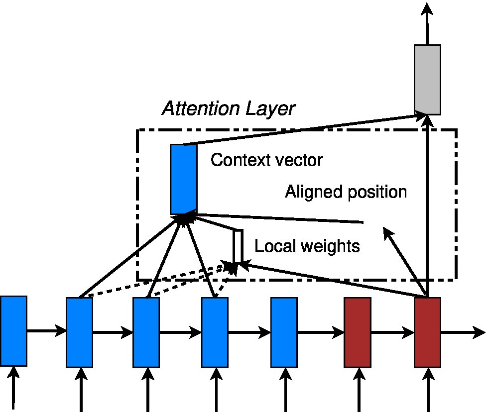
Figure 3: Local attention model – the model first predicts a single aligned position $p_{t}$ for the current target word. A window centered around the source position $p_{t}$ is then used to compute a context vector \mbox{\boldmath{c}}_{t}, a weighted average of the source hidden states in the window. The weights \mbox{\boldmath{a}}_{t} are inferred from the current target state \mbox{\boldmath{h}}_{t} and those source states \mbox{\boldmath{\bar{h}}}_{s} in the window.

图 3：局部注意力模型——模型首先为当前目标词预测一个对齐位置 $p_{t}$。然后用以源位置 $p_{t}$ 为中心的窗口计算上下文向量 \mbox{\boldmath{c}}_{t}，即窗口内源隐状态的加权平均。权重 \mbox{\boldmath{a}}_{t} 由当前目标状态 \mbox{\boldmath{h}}_{t} 以及窗口内那些源状态 \mbox{\boldmath{\bar{h}}}_{s} 推断得到。

The global attention has a drawback that it has to attend to all words on the source side for each target word, which is expensive and can potentially render it impractical to translate longer sequences, e.g., paragraphs or documents. To address this deficiency, we propose a local attentional mechanism that chooses to focus only on a small subset of the source positions per target word.

全局注意力的一个缺点是：对每个目标词都要关注源端的全部词，计算代价高，在翻译段落或文档等更长序列时，有可能变得不实用。为弥补这一不足，我们提出一种局部注意力机制，对每个目标词只选择关注源位置的一个小子集。

This model takes inspiration from the tradeoff between the soft and hard attentional models proposed by ?) to tackle the image caption generation task. In their work, soft attention refers to the global attention approach in which weights are placed “softly” over all patches in the source image. The hard attention, on the other hand, selects one patch of the image to attend to at a time. While less expensive at inference time, the hard attention model is non-differentiable and requires more complicated techniques such as variance reduction or reinforcement learning to train.

这一模型的灵感，来自 Xu 等人为图像描述生成任务提出的软注意力与硬注意力之间的折中。在他们的工作中，软注意力指的就是全局注意力方法，把权重“软地”放在源图像的所有块上。硬注意力则每次只选择图像中的一个块来关注。硬注意力在推理时更省计算，但不可微，训练时需要方差缩减或强化学习等更复杂的技术。

Our local attention mechanism selectively focuses on a small window of context and is differentiable. This approach has an advantage of avoiding the expensive computation incurred in the soft attention and at the same time, is easier to train than the hard attention approach. In concrete details, the model first generates an aligned position $p_{t}$ for each target word at time $t$. The context vector \mbox{\boldmath{c}}_{t} is then derived as a weighted average over the set of source hidden states within the window $[p_{t}-D,p_{t}+D]$; $D$ is empirically selected.[^8] Unlike the global approach, the local alignment vector \mbox{\boldmath{a}}_{t} is now fixed-dimensional, i.e., $\in\mathbb{R}^{2D+1}$. We consider two variants of the model as below.

[^8]: If the window crosses the sentence boundaries, we simply ignore the outside part and consider words in the window.

我们的局部注意力机制有选择地关注一小段上下文窗口，并且是可微的。这一方法的优点是：既避免了软注意力中昂贵的计算，又比硬注意力更容易训练。具体来说，模型首先为时刻 $t$ 的每个目标词生成一个对齐位置 $p_{t}$。然后，上下文向量 \mbox{\boldmath{c}}_{t} 取窗口 $[p_{t}-D,p_{t}+D]$ 内源隐状态的加权平均；$D$ 由经验选定。^8 与全局方法不同，局部对齐向量 \mbox{\boldmath{a}}_{t} 现在是固定维的，即 $\in\mathbb{R}^{2D+1}$。我们考虑如下两种变体。

Monotonic alignment (local-m) – we simply set $p_{t}\!=\!t$ assuming that source and target sequences are roughly monotonically aligned. The alignment vector \mbox{\boldmath{a}}_{t} is defined according to Eq. (7).[^9]

[^9]: local-m is the same as the global model except that the vector \mbox{\boldmath{a}}_{t} is fixed-length and shorter.

单调对齐（local-m）——我们简单地令 $p_{t}\!=\!t$，假定源序列与目标序列大致单调对齐。对齐向量 \mbox{\boldmath{a}}_{t} 按式（7）定义。[^9]

[^9]: local-m 与全局模型相同，只是向量 \mbox{\boldmath{a}}_{t} 长度固定且更短。

Predictive alignment (local-p) – instead of assuming monotonic alignments, our model predicts an aligned position as follows:

预测对齐（local-p）——不再假定单调对齐，我们的模型按如下方式预测对齐位置：

p_{t}=S\cdot\sigmoid(\mbox{\boldmath{$v$}}_{p}^{\top}\tanh(\mbox{\boldmath{$W_{p}$}}\mbox{\boldmath{$h$}}_{t})), \tag{9}

$W_{p}$ and \mbox{\boldmath{v}}_{p} are the model parameters which will be learned to predict positions. $S$ is the source sentence length. As a result of $\sigmoid$, $p_{t}\in[0,S]$. To favor alignment points near $p_{t}$, we place a Gaussian distribution centered around $p_{t}$ . Specifically, our alignment weights are now defined as:

$W_{p}$ 和 \mbox{\boldmath{v}}_{p} 是将要学习的、用于预测位置的模型参数。$S$ 是源句长度。由于使用了 $\sigmoid$，$p_{t}\in[0,S]$。为了偏向靠近 $p_{t}$ 的对齐点，我们在 $p_{t}$ 周围放置一个高斯分布。具体而言，对齐权重现在定义为：

\mbox{\boldmath{$a$}}_{t}(s)=\alignf(\mbox{\boldmath{$h$}}_{t},\mbox{\boldmath{$\bar{h}$}}_{s})\exp\left(-\frac{(s-p_{t})^{2}}{2\sigma^{2}}\right) \tag{10}

We use the same $\alignf$ function as in Eq. (7) and the standard deviation is empirically set as $\sigma\!=\!\frac{D}{2}$. Note that $p_{t}$ is a real nummber; whereas $s$ is an integer within the window centered at $p_{t}$.[^10]

[^10]: local-p is similar to the local-m model except that we dynamically compute $p_{t}$ and use a truncated Gaussian distribution to modify the original alignment weights as shown in Eq. (10). By utilizing $p_{t}$ to derive \mbox{\boldmath{a}}_{t}, we can compute backprop gradients for $W_{p}$ and \mbox{\boldmath{v}}_{p}. This model is differentiable almost everywhere.

我们使用与式（7）相同的 $\alignf$ 函数，并把标准差经验地设为 $\sigma\!=\!\frac{D}{2}$。注意 $p_{t}$ 是一个实数；而 $s$ 是以 $p_{t}$ 为中心的窗口内的整数。[^10]

[^10]: local-p 与 local-m 模型相似，不同之处在于我们动态计算 $p_{t}$，并用截断高斯分布按式（10）修正原来的对齐权重。借助 $p_{t}$ 来得到 \mbox{\boldmath{a}}_{t}，我们可以对 $W_{p}$ 和 \mbox{\boldmath{v}}_{p} 计算反向传播梯度。这一模型几乎处处可微。

Comparison to [Gregor et al. (2015] – have proposed a selective attention mechanism, very similar to our local attention, for the image generation task. Their approach allows the model to select an image patch of varying location and zoom. We, instead, use the same “zoom” for all target positions, which greatly simplifies the formulation and still achieves good performance.

与 [Gregor et al. (2015] 的比较——他们提出了一种选择性注意力机制，与我们的局部注意力非常相似，用于图像生成任务。他们的方法允许模型选择位置和缩放都可变的图像块。我们则对所有目标位置使用相同的“缩放”，这大大简化了公式，并且仍然能取得好的性能。

3.3 Input-feeding Approach

3.3 输入反馈方法

In our proposed global and local approaches, the attentional decisions are made independently, which is suboptimal. Whereas, in standard MT, a coverage set is often maintained during the translation process to keep track of which source words have been translated. Likewise, in attentional NMTs, alignment decisions should be made jointly taking into account past alignment information. To address that, we propose an input-feeding approach in which attentional vectors \mbox{\boldmath{\tilde{h}}}_{t} are concatenated with inputs at the next time steps as illustrated in Figure 4.[^11] The effects of having such connections are two-fold: (a) we hope to make the model fully aware of previous alignment choices and (b) we create a very deep network spanning both horizontally and vertically.

[^11]: If $n$ is the number of LSTM cells, the input size of the first LSTM layer is $2n$; those of subsequent layers are $n$.

在我们提出的全局和局部方法中，注意力决策是独立做出的，这并不是最优的。而在常规机器翻译中，翻译过程里常常维护一个覆盖集合，用来跟踪哪些源词已经被翻译。同样，在带注意力的 NMT 中，对齐决策应当联合考虑过去的对齐信息。为此，我们提出一种输入反馈方法：把注意力向量 \mbox{\boldmath{\tilde{h}}}_{t} 与下一时间步的输入拼接，如图 4 所示。[^11] 这样的连接有两方面作用：（a）我们希望模型充分了解先前的对齐选择；（b）我们得到一个在水平和垂直方向都延伸很深的网络。

[^11]: 若 $n$ 是 LSTM 单元数，则第一层 LSTM 的输入大小为 $2n$，后续各层为 $n$。

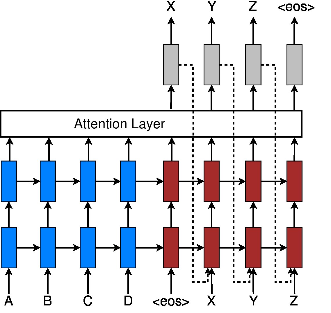
Figure 4: Input-feeding approach – Attentional vectors \mbox{\boldmath{\tilde{h}}}_{t} are fed as inputs to the next time steps to inform the model about past alignment decisions.

图 4：输入反馈方法——把注意力向量 \mbox{\boldmath{\tilde{h}}}_{t} 作为后续时间步的输入，让模型获知过去的对齐决策。

Comparison to other work – ?) use context vectors, similar to our \mbox{\boldmath{c}}_{t}, in building subsequent hidden states, which can also achieve the “coverage” effect. However, there has not been any analysis of whether such connections are useful as done in this work. Also, our approach is more general; as illustrated in Figure 4, it can be applied to general stacking recurrent architectures, including non-attentional models.

与其他工作的比较——Bahdanau 等人在构建后续隐状态时使用了与我们的 \mbox{\boldmath{c}}_{t} 类似的上下文向量，也可以达到“覆盖”效果。不过，此前还没有像本工作这样分析这些连接是否有用。此外，我们的方法更一般：如图 4 所示，它可以用于一般的堆叠循环结构，包括无注意力的模型。

?) propose a doubly attentional approach with an additional constraint added to the training objective to make sure the model pays equal attention to all parts of the image during the caption generation process. Such a constraint can also be useful to capture the coverage set effect in NMT that we mentioned earlier. However, we chose to use the input-feeding approach since it provides flexibility for the model to decide on any attentional constraints it deems suitable.

Xu 等人提出一种双重注意力方法，在训练目标中增加一条约束，以确保模型在图像描述生成过程中对图像各部分给予同等关注。这样的约束对于捕捉我们前面提到的 NMT 覆盖集合效果也可能有用。不过我们选择使用输入反馈方法，因为它让模型可以灵活决定自己认为合适的任何注意力约束。

4 Experiments

4 实验

We evaluate the effectiveness of our models on the WMT translation tasks between English and German in both directions. newstest2013 (3000 sentences) is used as a development set to select our hyperparameters. Translation performances are reported in case-sensitive BLEU [Papineni et al. (2002] on newstest2014 (2737 sentences) and newstest2015 (2169 sentences). Following [Luong et al. (2015], we report translation quality using two types of BLEU: (a) tokenized[^12] BLEU to be comparable with existing NMT work and (b) NIST[^13] BLEU to be comparable with WMT results.

[^12]: All texts are tokenized with tokenizer.perl and BLEU scores are computed with multi-bleu.perl.

[^13]: With the mteval-v13a script as per WMT guideline.

我们在 WMT 英德双向翻译任务上评估模型的有效性。newstest2013（3000 句）用作开发集，以选择超参数。翻译表现以区分大小写的 BLEU [Papineni et al. (2002] 在 newstest2014（2737 句）和 newstest2015（2169 句）上报告。沿用 [Luong et al. (2015]，我们用两类 BLEU 报告翻译质量：（a）分词后的[^12] BLEU，以便与已有 NMT 工作比较；（b）NIST[^13] BLEU，以便与 WMT 结果比较。

[^12]: 所有文本用 tokenizer.perl 分词，BLEU 分数用 multi-bleu.perl 计算。

[^13]: 按 WMT 规范使用 mteval-v13a 脚本。

System	Ppl	BLEU
Winning WMT’14 system – phrase-based + large LM [Buck et al. (2014]		20.7
Existing NMT systems
RNNsearch [Jean et al. (2015]		16.5
RNNsearch + unk replace [Jean et al. (2015]		19.0
RNNsearch + unk replace + large vocab + ensemble 8 models [Jean et al. (2015]		21.6
Our NMT systems
Base	10.6	11.3
Base + reverse	9.9	12.6 (+1.3)
Base + reverse + dropout	8.1	14.0 (+1.4)
Base + reverse + dropout + global attention (location)	7.3	16.8 (+2.8)
Base + reverse + dropout + global attention (location) + feed input	6.4	18.1 (+1.3)
Base + reverse + dropout + local-p attention (general) + feed input	5.9	19.0 (+0.9)
Base + reverse + dropout + local-p attention (general) + feed input + unk replace	20.9 (+1.9)
Ensemble 8 models + unk replace		23.0 (+2.1)

Table 1: WMT’14 English-German results – shown are the perplexities (ppl) and the tokenized BLEU scores of various systems on newstest2014. We highlight the best system in bold and give progressive improvements in italic between consecutive systems. local-p referes to the local attention with predictive alignments. We indicate for each attention model the alignment score function used in pararentheses.

系统	困惑度	BLEU
WMT’14 获胜系统——基于短语 + 大型语言模型 [Buck et al. (2014]		20.7
已有 NMT 系统
RNNsearch [Jean et al. (2015]		16.5
RNNsearch + unk 替换 [Jean et al. (2015]		19.0
RNNsearch + unk 替换 + 大词表 + 集成 8 个模型 [Jean et al. (2015]		21.6
我们的 NMT 系统
Base	10.6	11.3
Base + 反向	9.9	12.6（+1.3）
Base + 反向 + dropout	8.1	14.0（+1.4）
Base + 反向 + dropout + 全局注意力（location）	7.3	16.8（+2.8）
Base + 反向 + dropout + 全局注意力（location）+ 输入反馈	6.4	18.1（+1.3）
Base + 反向 + dropout + local-p 注意力（general）+ 输入反馈	5.9	19.0（+0.9）
Base + 反向 + dropout + local-p 注意力（general）+ 输入反馈 + unk 替换	20.9（+1.9）
集成 8 个模型 + unk 替换		23.0（+2.1）

表 1：WMT’14 英译德结果——给出各系统在 newstest2014 上的困惑度（ppl）和分词后 BLEU。我们把最好的系统加粗，并在连续系统之间用斜体标出逐步改进。local-p 指带预测对齐的局部注意力。我们在括号中标明每个注意力模型使用的对齐评分函数。

4.1 Training Details

4.1 训练细节

All our models are trained on the WMT’14 training data consisting of 4.5M sentences pairs (116M English words, 110M German words). Similar to [Jean et al. (2015], we limit our vocabularies to be the top 50K most frequent words for both languages. Words not in these shortlisted vocabularies are converted into a universal token $<$unk$>$.

我们的全部模型都在 WMT’14 训练数据上训练，包含 450 万句对（1.16 亿英语词，1.10 亿德语词）。与 [Jean et al. (2015] 类似，英德两边的词表都限制为最频繁的 5 万词。不在这份短名单中的词被转换成通用标记 $<$unk$>$。

When training our NMT systems, following [Bahdanau et al. (2015, Jean et al. (2015], we filter out sentence pairs whose lengths exceed 50 words and shuffle mini-batches as we proceed. Our stacking LSTM models have 4 layers, each with 1000 cells, and 1000-dimensional embeddings. We follow [Sutskever et al. (2014, Luong et al. (2015] in training NMT with similar settings: (a) our parameters are uniformly initialized in $[-0.1,0.1]$, (b) we train for 10 epochs using plain SGD, (c) a simple learning rate schedule is employed – we start with a learning rate of 1; after 5 epochs, we begin to halve the learning rate every epoch, (d) our mini-batch size is 128, and (e) the normalized gradient is rescaled whenever its norm exceeds 5. Additionally, we also use dropout with probability $0.2$ for our LSTMs as suggested by [Zaremba et al. (2015]. For dropout models, we train for 12 epochs and start halving the learning rate after 8 epochs. For local attention models, we empirically set the window size $D=10$.

训练 NMT 系统时，我们沿用 [Bahdanau et al. (2015, Jean et al. (2015]，过滤掉长度超过 50 词的句对，并在进行过程中打乱小批量。我们的堆叠 LSTM 模型有 4 层，每层 1000 个单元，词嵌入为 1000 维。我们按 [Sutskever et al. (2014, Luong et al. (2015] 用相近的设置训练 NMT：（a）参数在 $[-0.1,0.1]$ 上均匀初始化；（b）用普通 SGD 训练 10 个周期；（c）采用简单的学习率安排——起始学习率为 1；5 个周期之后，每个周期把学习率减半；（d）小批量大小为 128；（e）当归一化梯度的范数超过 5 时重新缩放。此外，我们还按 [Zaremba et al. (2015] 的建议，对 LSTM 使用概率为 $0.2$ 的 dropout。对使用 dropout 的模型，我们训练 12 个周期，并在 8 个周期之后开始把学习率减半。对局部注意力模型，我们经验地把窗口大小设为 $D=10$。

Our code is implemented in MATLAB. When running on a single GPU device Tesla K40, we achieve a speed of 1K target words per second. It takes 7–10 days to completely train a model.

我们的代码用 MATLAB 实现。在单块 Tesla K40 GPU 上运行时，速度达到每秒 1000 个目标词。完整训练一个模型需要 7–10 天。

4.2 English-German Results

4.2 英译德结果

We compare our NMT systems in the English-German task with various other systems. These include the winning system in WMT’14 [Buck et al. (2014], a phrase-based system whose language models were trained on a huge monolingual text, the Common Crawl corpus. For end-to-end NMT systems, to the best of our knowledge, [Jean et al. (2015] is the only work experimenting with this language pair and currently the SOTA system. We only present results for some of our attention models and will later analyze the rest in Section 5.

我们在英译德任务上把我们的 NMT 系统与其他多种系统比较。其中包括 WMT’14 的获胜系统 [Buck et al. (2014]，这是一套基于短语的系统，其语言模型在海量单语文本 Common Crawl 语料上训练。对端到端 NMT 系统，据我们所知，[Jean et al. (2015] 是唯一在这一语言对上做实验的工作，也是当时最好的系统。我们只给出部分注意力模型的结果，其余将在第 5 节再分析。

As shown in Table 1, we achieve progressive improvements when (a) reversing the source sentence, +$1.3$ BLEU, as proposed in [Sutskever et al. (2014] and (b) using dropout, +$1.4$ BLEU. On top of that, (c) the global attention approach gives a significant boost of +$2.8$ BLEU, making our model slightly better than the base attentional system of ?) (row RNNSearch). When (d) using the input-feeding approach, we seize another notable gain of +$1.3$ BLEU and outperform their system. The local attention model with predictive alignments (row local-p) proves to be even better, giving us a further improvement of +$0.9$ BLEU on top of the global attention model. It is interesting to observe the trend previously reported in [Luong et al. (2015] that perplexity strongly correlates with translation quality. In total, we achieve a significant gain of 5.0 BLEU points over the non-attentional baseline, which already includes known techniques such as source reversing and dropout.

如表 1 所示，当我们（a）按 [Sutskever et al. (2014] 的建议把源句反向，得到 +$1.3$ BLEU，以及（b）使用 dropout，得到 +$1.4$ BLEU 时，分数逐步提高。在此之上，（c）全局注意力方法又带来 +$2.8$ BLEU 的显著提升，使我们的模型略好于 Jean 等人的基础注意力系统（RNNSearch 一行）。当（d）使用输入反馈方法时，我们又获得 +$1.3$ BLEU 的可观增益，并超过他们的系统。带预测对齐的局部注意力模型（local-p 一行）更好，在全局注意力之上再提升 +$0.9$ BLEU。有意思的是，我们可以看到 [Luong et al. (2015] 中报告过的趋势：困惑度与翻译质量密切相关。合计起来，相对已经包含源句反向和 dropout 等已知技术的无注意力基线，我们取得了 5.0 BLEU 的显著提升。

The unknown replacement technique proposed in [Luong et al. (2015, Jean et al. (2015] yields another nice gain of +$1.9$ BLEU, demonstrating that our attentional models do learn useful alignments for unknown works. Finally, by ensembling 8 different models of various settings, e.g., using different attention approaches, with and without dropout etc., we were able to achieve a new SOTA result of $23.0{}$ BLEU, outperforming the existing best system [Jean et al. (2015] by +$1.4$ BLEU.

[Luong et al. (2015, Jean et al. (2015] 提出的未知词替换技术又带来 +$1.9$ BLEU 的可喜增益，说明我们的注意力模型确实为未知词学到了有用的对齐。最后，通过把 8 个不同设置的模型集成起来，例如使用不同的注意力方法、有无 dropout 等，我们得到了 $23.0{}$ BLEU 的新的当时最好结果，比当时最好的系统 [Jean et al. (2015] 高出 +$1.4$ BLEU。

System	BLEU
Top – NMT + 5-gram rerank (Montreal)	24.9
Our ensemble 8 models + unk replace	25.9

Table 2: WMT’15 English-German results – NIST BLEU scores of the winning entry in WMT’15 and our best one on newstest2015.

系统	BLEU
最好——NMT + 5 元重排序（Montreal）	24.9
我们集成 8 个模型 + unk 替换	25.9

表 2：WMT’15 英译德结果——WMT’15 获胜条目与我们最好系统在 newstest2015 上的 NIST BLEU 分数。

Latest results in WMT’15 – despite the fact that our models were trained on WMT’14 with slightly less data, we test them on newstest2015 to demonstrate that they can generalize well to different test sets. As shown in Table 2, our best system establishes a new SOTA performance of $25.9{}$ BLEU, outperforming the existing best system backed by NMT and a 5-gram LM reranker by +$1.0$ BLEU.

WMT’15 的最新结果——尽管我们的模型是在数据稍少的 WMT’14 上训练的，我们仍在 newstest2015 上测试，以表明它们能够很好地泛化到不同测试集。如表 2 所示，我们最好的系统达到 $25.9{}$ BLEU 的新的当时最好成绩，比由 NMT 加 5 元语言模型重排序支撑的已有最好系统高出 +$1.0$ BLEU。

4.3 German-English Results

4.3 德译英结果

We carry out a similar set of experiments for the WMT’15 translation task from German to English. While our systems have not yet matched the performance of the SOTA system, we nevertheless show the effectiveness of our approaches with large and progressive gains in terms of BLEU as illustrated in Table 3. The attentional mechanism gives us +$2.2$ BLEU gain and on top of that, we obtain another boost of up to +$1.0$ BLEU from the input-feeding approach. Using a better alignment function, the content-based dot product one, together with dropout yields another gain of +$2.7$ BLEU. Lastly, when applying the unknown word replacement technique, we seize an additional +$2.1$ BLEU, demonstrating the usefulness of attention in aligning rare words.

我们对 WMT’15 德译英任务做了一组类似的实验。虽然我们的系统尚未达到当时最好系统的水平，但如表 3 所示，我们仍以 BLEU 上大幅且逐步的提升展示了方法的有效性。注意力机制带来 +$2.2$ BLEU，在此之上，输入反馈方法再给出最高 +$1.0$ BLEU 的提升。使用更好的对齐函数，即基于内容的 dot 乘积，再加上 dropout，又获得 +$2.7$ BLEU。最后，采用未知词替换技术后再增加 +$2.1$ BLEU，说明注意力在对齐罕见词上很有用。

5 Analysis

5 分析

We conduct extensive analysis to better understand our models in terms of learning, the ability to handle long sentences, choices of attentional architectures, and alignment quality. All results reported here are on English-German newstest2014.

我们做了详尽分析，以便更好地理解模型在学习过程、处理长句的能力、注意力结构选择以及对齐质量等方面的表现。这里报告的全部结果都基于英译德 newstest2014。

System	Ppl.	BLEU
WMT’15 systems
SOTA – phrase-based (Edinburgh)		29.2
NMT + 5-gram rerank (MILA)		27.6
Our NMT systems
Base (reverse)	14.3	16.9
+ global (location)	12.7	19.1 (+2.2)
+ global (location) + feed	10.9	20.1 (+1.0)
+ global (dot) + drop + feed	9.7	22.8 (+2.7)
+ global (dot) + drop + feed + unk	24.9 (+2.1)

Table 3: WMT’15 German-English results – performances of various systems (similar to Table 1). The base system already includes source reversing on which we add global attention, dropout, input feeding, and unk replacement.

系统	困惑度	BLEU
WMT’15 系统
当时最好——基于短语（Edinburgh）		29.2
NMT + 5 元重排序（MILA）		27.6
我们的 NMT 系统
Base（反向）	14.3	16.9
+ 全局（location）	12.7	19.1（+2.2）
+ 全局（location）+ 反馈	10.9	20.1（+1.0）
+ 全局（dot）+ dropout + 反馈	9.7	22.8（+2.7）
+ 全局（dot）+ dropout + 反馈 + unk	24.9（+2.1）

表 3：WMT’15 德译英结果——各系统的表现（与表 1 类似）。基线系统已经包含源句反向，我们再依次加入全局注意力、dropout、输入反馈和 unk 替换。

5.1 Learning curves

5.1 学习曲线

We compare models built on top of one another as listed in Table 1. It is pleasant to observe in Figure 5 a clear separation between non-attentional and attentional models. The input-feeding approach and the local attention model also demonstrate their abilities in driving the test costs lower. The non-attentional model with dropout (the blue + curve) learns slower than other non-dropout models, but as time goes by, it becomes more robust in terms of minimizing test errors.

我们比较了表 1 中层层叠加的模型。令人满意的是，图 5 中无注意力模型与注意力模型之间有清楚的分界。输入反馈方法和局部注意力模型也展示了把测试代价进一步压低的能力。带 dropout 的无注意力模型（蓝色 + 曲线）比其他不使用 dropout 的模型学得更慢，但随着时间推移，它在降低测试误差上变得更稳健。

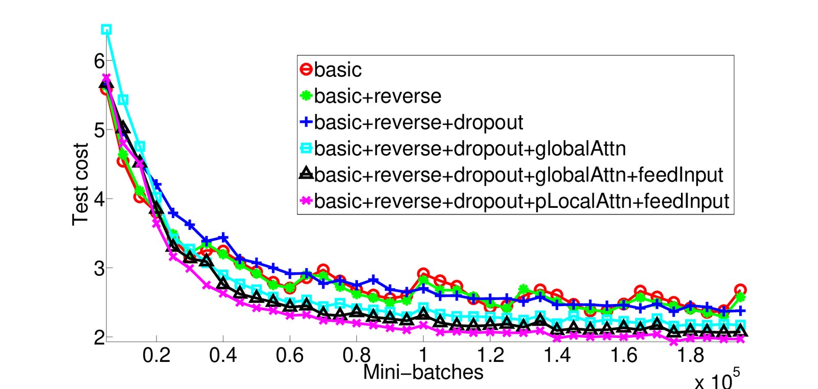
Figure 5: Learning curves – test cost ($\ln$ perplexity) on newstest2014 for English-German NMTs as training progresses.

图 5：学习曲线——英译德 NMT 在 newstest2014 上的测试代价（$\ln$ 困惑度）随训练进行的变化。

5.2 Effects of Translating Long Sentences

5.2 翻译长句的效果

We follow [Bahdanau et al. (2015] to group sentences of similar lengths together and compute a BLEU score per group. Figure 6 shows that our attentional models are more effective than the non-attentional one in handling long sentences: the quality does not degrade as sentences become longer. Our best model (the blue + curve) outperforms all other systems in all length buckets.

我们按 [Bahdanau et al. (2015] 的做法，把长度相近的句子分组，并为每组计算 BLEU。图 6 表明，我们的注意力模型在处理长句上比无注意力模型更有效：句子变长时质量不会下降。我们最好的模型（蓝色 + 曲线）在所有长度区间上都超过其他系统。

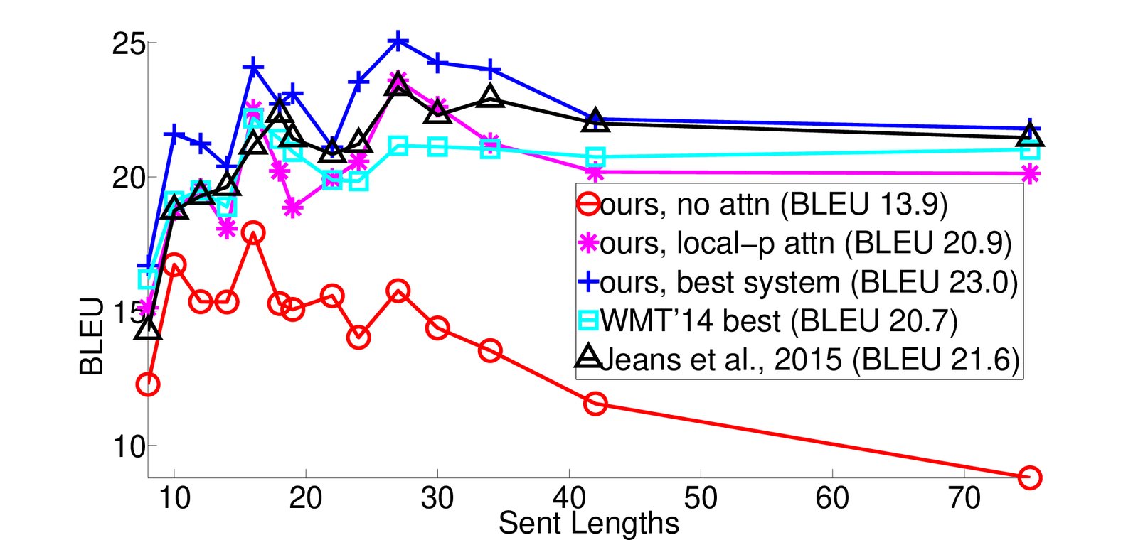
Figure 6: Length Analysis – translation qualities of different systems as sentences become longer.

图 6：长度分析——不同系统的翻译质量随句子变长的变化。

5.3 Choices of Attentional Architectures

5.3 注意力结构的选择

We examine different attention models (global, local-m, local-p) and different alignment functions (location, dot, general, concat) as described in Section 3. Due to limited resources, we cannot run all the possible combinations. However, results in Table 4 do give us some idea about different choices. The location-based function does not learn good alignments: the global (location) model can only obtain a small gain when performing unknown word replacement compared to using other alignment functions.[^14] For content-based functions, our implementation concat does not yield good performances and more analysis should be done to understand the reason.[^15] It is interesting to observe that dot works well for the global attention and general is better for the local attention. Among the different models, the local attention model with predictive alignments (local-p) is best, both in terms of perplexities and BLEU.

[^14]: There is a subtle difference in how we retrieve alignments for the different alignment functions. At time step $t$ in which we receive $y_{t-1}$ as input and then compute \mbox{\boldmath{h}}_{t},\mbox{\boldmath{a}}_{t},\mbox{\boldmath{c}}_{t}, and \mbox{\boldmath{\tilde{h}}}_{t} before predicting $y_{t}$, the alignment vector \mbox{\boldmath{a}}_{t} is used as alignment weights for (a) the predicted word $y_{t}$ in the location-based alignment functions and (b) the input word $y_{t-1}$ in the content-based functions.

[^15]: With concat, the perplexities achieved by different models are 6.7 (global), 7.1 (local-m), and 7.1 (local-p). Such high perplexities could be due to the fact that we simplify the matrix $W_{a}$ to set the part that corresponds to \mbox{\boldmath{\bar{h}}}_{s} to identity.

我们考察了第 3 节中描述的不同注意力模型（global、local-m、local-p）和不同对齐函数（location、dot、general、concat）。由于资源有限，我们无法跑完所有可能的组合。不过，表 4 中的结果仍能让我们对不同选择有一些认识。基于位置的函数没有学到好的对齐：与使用其他对齐函数相比，global (location) 模型在做未知词替换时只能获得较小的增益。[^14] 对基于内容的函数，我们实现的 concat 没有给出好的性能，其原因还需要更多分析。[^15] 有意思的是，dot 对全局注意力效果更好，而 general 对局部注意力更好。在不同模型中，带预测对齐的局部注意力模型（local-p）最好，无论是困惑度还是 BLEU。

[^14]: 不同对齐函数在提取对齐时有一个细微差别。在时间步 $t$，模型接收 $y_{t-1}$ 作为输入，再计算 \mbox{\boldmath{h}}_{t},\mbox{\boldmath{a}}_{t},\mbox{\boldmath{c}}_{t} 和 \mbox{\boldmath{\tilde{h}}}_{t}，然后预测 $y_{t}$。对齐向量 \mbox{\boldmath{a}}_{t} 被用作对齐权重的方式是：（a）在基于位置的对齐函数中，对应预测词 $y_{t}$；（b）在基于内容的函数中，对应输入词 $y_{t-1}$。

[^15]: 使用 concat 时，不同模型达到的困惑度为 6.7（global）、7.1（local-m）和 7.1（local-p）。如此高的困惑度，可能是因为我们简化了矩阵 $W_{a}$，把对应于 \mbox{\boldmath{\bar{h}}}_{s} 的那一部分设成了单位阵。

System	Ppl	BLEU
Before	After unk
global (location)	6.4	18.1	19.3 (+1.2)
global (dot)	6.1	18.6	20.5 (+1.9)
global (general)	6.1	17.3	19.1 (+1.8)
local-m (dot)	$>$7.0	x	x
local-m (general)	6.2	18.6	20.4 (+1.8)
local-p (dot)	6.6	18.0	19.6 (+1.9)
local-p (general)	5.9	19	20.9 (+1.9)

Table 4: Attentional Architectures – performances of different attentional models. We trained two local-m (dot) models; both have ppl $>7.0$.

系统	困惑度	BLEU
替换前	替换 unk 后
global (location)	6.4	18.1	19.3（+1.2）
global (dot)	6.1	18.6	20.5（+1.9）
global (general)	6.1	17.3	19.1（+1.8）
local-m (dot)	$>7.0$	x	x
local-m (general)	6.2	18.6	20.4（+1.8）
local-p (dot)	6.6	18.0	19.6（+1.9）
local-p (general)	5.9	19	20.9（+1.9）

表 4：注意力结构——不同注意力模型的表现。我们训练了两个 local-m (dot) 模型，二者的困惑度都 $>7.0$。

English-German translations
src	Orlando Bloom and Miranda Kerr still love each other
ref	Orlando Bloom und Miranda Kerr lieben sich noch immer
best	Orlando Bloom und Miranda Kerr lieben einander noch immer .
base	Orlando Bloom und Lucas Miranda lieben einander noch immer .
src	′′ We ′ re pleased the FAA recognizes that an enjoyable passenger experience is not incompatible with safety and security , ′′ said Roger Dow , CEO of the U.S. Travel Association .
ref	“ Wir freuen uns , dass die FAA erkennt , dass ein angenehmes Passagiererlebnis nicht im Widerspruch zur Sicherheit steht ” , sagte Roger Dow , CEO der U.S. Travel Association .
best	′′ Wir freuen uns , dass die FAA anerkennt , dass ein angenehmes ist nicht mit Sicherheit und Sicherheit unvereinbar ist ′′ , sagte Roger Dow , CEO der US - die .
base	′′ Wir freuen uns über die $<$unk$>$ , dass ein $<$unk$>$ $<$unk$>$ mit Sicherheit nicht vereinbar ist mit Sicherheit und Sicherheit ′′ , sagte Roger Cameron , CEO der US - $<$unk$>$ .
German-English translations
src	In einem Interview sagte Bloom jedoch , dass er und Kerr sich noch immer lieben .
ref	However , in an interview , Bloom has said that he and Kerr still love each other .
best	In an interview , however , Bloom said that he and Kerr still love .
base	However , in an interview , Bloom said that he and Tina were still $<$unk$>$ .
src	Wegen der von Berlin und der Europäischen Zentralbank verhängten strengen Sparpolitik in Verbindung mit der Zwangsjacke , in die die jeweilige nationale Wirtschaft durch das Festhalten an der gemeinsamen Währung genötigt wird , sind viele Menschen der Ansicht , das Projekt Europa sei zu weit gegangen
ref	The austerity imposed by Berlin and the European Central Bank , coupled with the straitjacket imposed on national economies through adherence to the common currency , has led many people to think Project Europe has gone too far .
best	Because of the strict austerity measures imposed by Berlin and the European Central Bank in connection with the straitjacket in which the respective national economy is forced to adhere to the common currency , many people believe that the European project has gone too far .
base	Because of the pressure imposed by the European Central Bank and the Federal Central Bank with the strict austerity imposed on the national economy in the face of the single currency , many people believe that the European project has gone too far .

Table 5: Sample translations – for each example, we show the source (src), the human translation (ref), the translation from our best model (best), and the translation of a non-attentional model (base). We italicize some correct translation segments and highlight a few wrong ones in bold.

英译德翻译
源文	Orlando Bloom and Miranda Kerr still love each other
参考	Orlando Bloom und Miranda Kerr lieben sich noch immer
最好	Orlando Bloom und Miranda Kerr lieben einander noch immer .
基线	Orlando Bloom und Lucas Miranda lieben einander noch immer .
源文	′′ We ′ re pleased the FAA recognizes that an enjoyable passenger experience is not incompatible with safety and security , ′′ said Roger Dow , CEO of the U.S. Travel Association .
参考	“ Wir freuen uns , dass die FAA erkennt , dass ein angenehmes Passagiererlebnis nicht im Widerspruch zur Sicherheit steht ” , sagte Roger Dow , CEO der U.S. Travel Association .
最好	′′ Wir freuen uns , dass die FAA anerkennt , dass ein angenehmes ist nicht mit Sicherheit und Sicherheit unvereinbar ist ′′ , sagte Roger Dow , CEO der US - die .
基线	′′ Wir freuen uns über die $<$unk$>$ , dass ein $<$unk$>$ $<$unk$>$ mit Sicherheit nicht vereinbar ist mit Sicherheit und Sicherheit ′′ , sagte Roger Cameron , CEO der US - $<$unk$>$ .
德译英翻译
源文	In einem Interview sagte Bloom jedoch , dass er und Kerr sich noch immer lieben .
参考	However , in an interview , Bloom has said that he and Kerr still love each other .
最好	In an interview , however , Bloom said that he and Kerr still love .
基线	However , in an interview , Bloom said that he and Tina were still $<$unk$>$ .
源文	Wegen der von Berlin und der Europäischen Zentralbank verhängten strengen Sparpolitik in Verbindung mit der Zwangsjacke , in die die jeweilige nationale Wirtschaft durch das Festhalten an der gemeinsamen Währung genötigt wird , sind viele Menschen der Ansicht , das Projekt Europa sei zu weit gegangen
参考	The austerity imposed by Berlin and the European Central Bank , coupled with the straitjacket imposed on national economies through adherence to the common currency , has led many people to think Project Europe has gone too far .
最好	Because of the strict austerity measures imposed by Berlin and the European Central Bank in connection with the straitjacket in which the respective national economy is forced to adhere to the common currency , many people believe that the European project has gone too far .
基线	Because of the pressure imposed by the European Central Bank and the Federal Central Bank with the strict austerity imposed on the national economy in the face of the single currency , many people believe that the European project has gone too far .

表 5：翻译样例——对每个例子，我们给出源文（源文）、人工译文（参考）、我们最好模型的译文（最好），以及无注意力模型的译文（基线）。我们用斜体标出一些正确的翻译片段，并用粗体标出若干错误之处。

5.4 Alignment Quality

5.4 对齐质量

A by-product of attentional models are word alignments. While [Bahdanau et al. (2015] visualized alignments for some sample sentences and observed gains in translation quality as an indication of a working attention model, no work has assessed the alignments learned as a whole. In contrast, we set out to evaluate the alignment quality using the alignment error rate (AER) metric.

注意力模型的一个副产品是词对齐。尽管 [Bahdanau et al. (2015] 为一些样例句可视化了对齐，并把翻译质量的提升视为注意力模型起作用的迹象，但还没有工作从整体上评估学到的对齐。与之相对，我们着手用对齐错误率（AER）这一指标来评估对齐质量。

Method	AER
global (location)	$0.39$
local-m (general)	$0.34$
local-p (general)	$0.36$
ensemble	$0.34$
Berkeley Aligner	$0.32$

Table 6: AER scores – results of various models on the RWTH English-German alignment data.

方法	AER
global (location)	$0.39$
local-m (general)	$0.34$
local-p (general)	$0.36$
集成	$0.34$
Berkeley Aligner	$0.32$

表 6：AER 分数——各模型在 RWTH 英德对齐数据上的结果。

Given the gold alignment data provided by RWTH for 508 English-German Europarl sentences, we “force” decode our attentional models to produce translations that match the references. We extract only one-to-one alignments by selecting the source word with the highest alignment weight per target word. Nevertheless, as shown in Table 6, we were able to achieve AER scores comparable to the one-to-many alignments obtained by the Berkeley aligner [Liang et al. (2006].[^16]

[^16]: We concatenate the 508 sentence pairs with 1M sentence pairs from WMT and run the Berkeley aligner.

给定 RWTH 提供的 508 句英德欧洲议会语料的标准对齐数据，我们“强制”解码注意力模型，使其译文与参考译文一致。对每个目标词，我们只选取对齐权重最高的那个源词，从而只提取一对一对齐。尽管如此，如表 6 所示，我们仍能得到与 Berkeley aligner [Liang et al. (2006] 得到的一对多对齐相当的 AER 分数。[^16]

[^16]: 我们把这 508 个句对与来自 WMT 的 100 万句对拼接，再运行 Berkeley aligner。

We also found that the alignments produced by local attention models achieve lower AERs than those of the global one. The AER obtained by the ensemble, while good, is not better than the local-m AER, suggesting the well-known observation that AER and translation scores are not well correlated [Fraser and Marcu (2007]. We show some alignment visualizations in Appendix A.

我们还发现，局部注意力模型产生的对齐，其 AER 低于全局模型。集成模型得到的 AER 虽然不错，但并不好于 local-m 的 AER，这印证了一个广为人知的观察：AER 与翻译分数并不是很好地相关 [Fraser and Marcu (2007]。我们在附录 A 中给出一些对齐可视化。

5.5 Sample Translations

5.5 翻译样例

We show in Table 5 sample translations in both directions. It it appealing to observe the effect of attentional models in correctly translating names such as “Miranda Kerr” and “Roger Dow”. Non-attentional models, while producing sensible names from a language model perspective, lack the direct connections from the source side to make correct translations. We also observed an interesting case in the second example, which requires translating the doubly-negated phrase, “not incompatible”. The attentional model correctly produces “nicht $\dots$ unvereinbar’’; whereas the non-attentional model generates ‘‘nicht vereinbar’’, meaning ‘‘not compatible’’.[^17] The attentional model also demonstrates its superiority in translating long sentences as in the last example.

[^17]: The reference uses a more fancy translation of “incompatible”, which is “im Widerspruch zu etwas stehen”. Both models, however, failed to translate “passenger experience”.

我们在表 5 中给出两个方向的翻译样例。可以看到，注意力模型能够正确翻译 “Miranda Kerr” 和 “Roger Dow” 这类人名，这一点很有吸引力。无注意力模型从语言模型的角度看也会生成说得通的名字，但缺少来自源端的直接连接，因而无法译对。我们还在第二个例子中看到一个有意思的情形，需要翻译双重否定短语 “not incompatible”。注意力模型正确地生成了 “nicht $\dots$ unvereinbar”；而无注意力模型生成了 “nicht vereinbar”，意思变成了 “不相容”。[^17] 在最后一个例子中，注意力模型在翻译长句上也表现出优势。

[^17]: 参考译文对 “incompatible” 用了更讲究的译法，即 “im Widerspruch zu etwas stehen”。不过两个模型都没能翻译出 “passenger experience”。

6 Conclusion

6 结论

In this paper, we propose two simple and effective attentional mechanisms for neural machine translation: the global approach which always looks at all source positions and the local one that only attends to a subset of source positions at a time. We test the effectiveness of our models in the WMT translation tasks between English and German in both directions. Our local attention yields large gains of up to $5.0{}$ BLEU over non-attentional models which already incorporate known techniques such as dropout. For the English to German translation direction, our ensemble model has established new state-of-the-art results for both WMT’14 and WMT’15, outperforming existing best systems, backed by NMT models and $n$-gram LM rerankers, by more than 1.0 BLEU.

本文为神经机器翻译提出两种简单而有效的注意力机制：全局方法始终察看所有源位置，局部方法每次只关注源位置的一个子集。我们在 WMT 英德双向翻译任务上检验了模型的有效性。我们的局部注意力相对已经加入 dropout 等已知技术的无注意力模型，最高可获得 $5.0{}$ BLEU 的大幅提升。在英译德方向，我们的集成模型在 WMT’14 和 WMT’15 上都树立了新的当时最好结果，比由 NMT 模型加 $n$ 元语言模型重排序支撑的已有最好系统高出 1.0 BLEU 以上。

We have compared various alignment functions and shed light on which functions are best for which attentional models. Our analysis shows that attention-based NMT models are superior to non-attentional ones in many cases, for example in translating names and handling long sentences.

我们比较了多种对齐函数，并说明哪些函数更适合哪些注意力模型。分析表明，基于注意力的 NMT 模型在许多情形下优于无注意力模型，例如在翻译人名和处理长句时。

Acknowledgment

致谢

We gratefully acknowledge support from a gift from Bloomberg L.P. and the support of NVIDIA Corporation with the donation of Tesla K40 GPUs. We thank Andrew Ng and his group as well as the Stanford Research Computing for letting us use their computing resources. We thank Russell Stewart for helpful discussions on the models. Lastly, we thank Quoc Le, Ilya Sutskever, Oriol Vinyals, Richard Socher, Michael Kayser, Jiwei Li, Panupong Pasupat, Kelvin Guu, members of the Stanford NLP Group and the annonymous reviewers for their valuable comments and feedback.

我们感谢 Bloomberg L.P. 的捐赠支持，以及 NVIDIA Corporation 捐赠 Tesla K40 GPU。我们感谢 Andrew Ng 及其小组以及 Stanford Research Computing，让我们使用他们的计算资源。我们感谢 Russell Stewart 就模型进行的有益讨论。最后，我们感谢 Quoc Le、Ilya Sutskever、Oriol Vinyals、Richard Socher、Michael Kayser、Jiwei Li、Panupong Pasupat、Kelvin Guu、Stanford NLP Group 的成员以及匿名审稿人提出的宝贵意见和反馈。

References

参考文献

[Bahdanau et al. (2015] D. Bahdanau, K. Cho, and Y. Bengio. 2015. Neural machine translation by jointly learning to align and translate. In ICLR .

[Buck et al. (2014] Christian Buck, Kenneth Heafield, and Bas van Ooyen. 2014. N-gram counts and language models from the common crawl. In LREC .

[Cho et al. (2014] Kyunghyun Cho, Bart van Merrienboer, Caglar Gulcehre, Fethi Bougares, Holger Schwenk, and Yoshua Bengio. 2014. Learning phrase representations using RNN encoder-decoder for statistical machine translation. In EMNLP .

[Fraser and Marcu (2007] Alexander Fraser and Daniel Marcu. 2007. Measuring word alignment quality for statistical machine translation. Computational Linguistics , 33(3):293–303.

[Gregor et al. (2015] Karol Gregor, Ivo Danihelka, Alex Graves, Danilo Jimenez Rezende, and Daan Wierstra. 2015. DRAW: A recurrent neural network for image generation. In ICML .

[Jean et al. (2015] Sébastien Jean, Kyunghyun Cho, Roland Memisevic, and Yoshua Bengio. 2015. On using very large target vocabulary for neural machine translation. In ACL .

[Kalchbrenner and Blunsom (2013] N. Kalchbrenner and P. Blunsom. 2013. Recurrent continuous translation models. In EMNLP .

[Koehn et al. (2003] Philipp Koehn, Franz Josef Och, and Daniel Marcu. 2003. Statistical phrase-based translation. In NAACL .

[Liang et al. (2006] P. Liang, B. Taskar, and D. Klein. 2006. Alignment by agreement. In NAACL .

[Luong et al. (2015] M.-T. Luong, I. Sutskever, Q. V. Le, O. Vinyals, and W. Zaremba. 2015. Addressing the rare word problem in neural machine translation. In ACL .

[Mnih et al. (2014] Volodymyr Mnih, Nicolas Heess, Alex Graves, and Koray Kavukcuoglu. 2014. Recurrent models of visual attention. In NIPS .

[Papineni et al. (2002] Kishore Papineni, Salim Roukos, Todd Ward, and Wei jing Zhu. 2002. Bleu: a method for automatic evaluation of machine translation. In ACL .

[Sutskever et al. (2014] I. Sutskever, O. Vinyals, and Q. V. Le. 2014. Sequence to sequence learning with neural networks. In NIPS .

[Xu et al. (2015] Kelvin Xu, Jimmy Ba, Ryan Kiros, Kyunghyun Cho, Aaron C. Courville, Ruslan Salakhutdinov, Richard S. Zemel, and Yoshua Bengio. 2015. Show, attend and tell: Neural image caption generation with visual attention. In ICML .

[Zaremba et al. (2015] Wojciech Zaremba, Ilya Sutskever, and Oriol Vinyals. 2015. Recurrent neural network regularization. In ICLR .

Appendix A Alignment Visualization

附录 A 对齐可视化

We visualize the alignment weights produced by our different attention models in Figure 7. The visualization of the local attention model is much sharper than that of the global one. This contrast matches our expectation that local attention is designed to only focus on a subset of words each time. Also, since we translate from English to German and reverse the source English sentence, the white strides at the words “reality” and “.” in the global attention model reveals an interesting access pattern: it tends to refer back to the beginning of the source sequence.

我们在图 7 中可视化了不同注意力模型产生的对齐权重。局部注意力模型的可视化比全局模型尖锐得多。这一对比符合我们的预期：局部注意力本就设计成每次只关注一个词子集。此外，由于我们是从英语译到德语，并把英语源句反向，全局注意力模型在 “reality” 和 “.” 这些词上出现的白色条带，揭示了一种有意思的访问模式：它往往回头去看源序列的开头。

Compared to the alignment visualizations in [Bahdanau et al. (2015], our alignment patterns are not as sharp as theirs. Such difference could possibly be due to the fact that translating from English to German is harder than translating into French as done in [Bahdanau et al. (2015], which is an interesting point to examine in future work.

与 [Bahdanau et al. (2015] 中的对齐可视化相比，我们的对齐模式不如他们的尖锐。这种差别可能是因为英译德比 [Bahdanau et al. (2015] 中的译入法语更难，这一点值得在未来工作中考察。

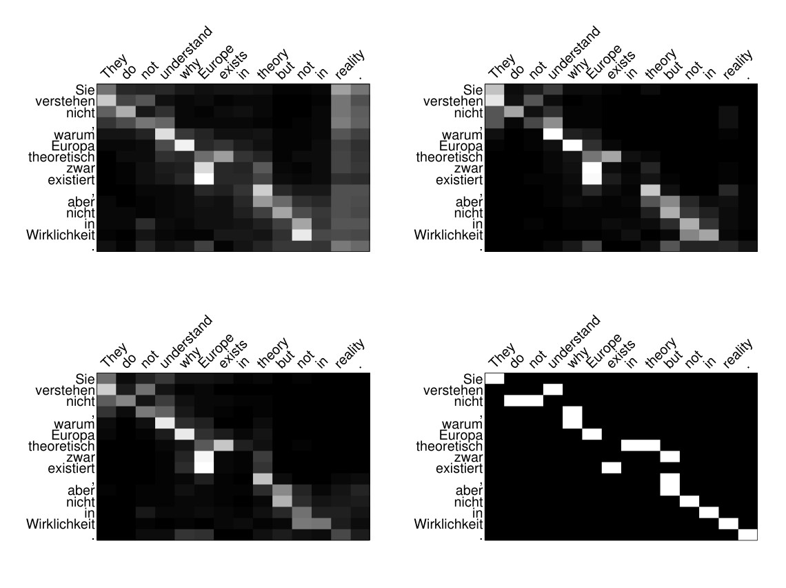
Figure 7: Alignment visualizations – shown are images of the attention weights learned by various models: (top left) global, (top right) local-m, and (bottom left) local-p. The gold alignments are displayed at the bottom right corner.

图 7：对齐可视化——给出各种模型学到的注意力权重图像：（左上）全局，（右上）local-m，（左下）local-p。标准对齐显示在右下角。