The Unreasonable Effectiveness of Deep Features as a Perceptual Metric
The Unreasonable Effectiveness of Deep Features as a Perceptual Metric
Abstract
摘要
While it is nearly effortless for humans to quickly assess the perceptual similarity between two images, the underlying processes are thought to be quite complex. Despite this, the most widely used perceptual metrics today, such as PSNR and SSIM, are simple, shallow functions, and fail to account for many nuances of human perception. Recently, the deep learning community has found that features of the VGG network trained on ImageNet classification has been remarkably useful as a training loss for image synthesis. But how perceptual are these so-called “perceptual losses”? What elements are critical for their success? To answer these questions, we introduce a new dataset of human perceptual similarity judgments. We systematically evaluate deep features across different architectures and tasks and compare them with classic metrics. We find that deep features outperform all previous metrics by large margins on our dataset. More surprisingly, this result is not restricted to ImageNet-trained VGG features, but holds across different deep architectures and levels of supervision (supervised, self-supervised, or even unsupervised). Our results suggest that perceptual similarity is an emergent property shared across deep visual representations.
人类几乎不费力就能迅速判断两张图像在感知上有多相似,但背后的过程通常被认为相当复杂。尽管如此,今天用得最广的感知度量,例如 PSNR 和 SSIM,仍是简单而浅层的函数,无法顾及人类感知中的许多细微之处。近来,深度学习社区发现,在 ImageNet 分类任务上训练的 VGG 网络特征,作为图像合成的训练损失格外好用。但这些所谓的“感知损失”到底有多“感知”?成功的关键又在哪里?为回答这些问题,我们引入一套新的人类感知相似度判断数据集。我们系统评估了不同架构和任务下的深度特征,并与经典度量作比较。我们发现,深度特征在该数据集上以较大幅度超过了以往所有度量。更出乎意料的是,这一结果并不限于在 ImageNet 上训练的 VGG 特征,而是在不同的深度架构和监督程度(监督、自监督,乃至无监督)上同样成立。我们的结果表明,感知相似度是深度视觉表示中共同涌现的一种性质。
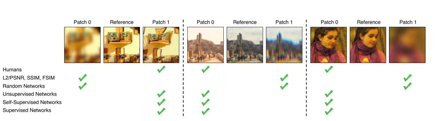
Figure 1: Which patch (left or right) is “closer” to the middle patch in these examples? In each case, the traditional metrics (L2/PSNR, SSIM, FSIM) disagree with human judgments. But deep networks, even across architectures (Squeezenet [20], AlexNet [27], VGG [51]) and supervision type (supervised [46], self-supervised [13, 40, 42, 63], and even unsupervised [26]), provide an emergent embedding which agrees surprisingly well with humans. We further calibrate existing deep embeddings on a large-scale database of perceptual judgments; models and data can be found at https://www.github.com/richzhang/PerceptualSimilarity.
图 1:在这些例子里,左边和右边哪一块与中间的参考块更“接近”?每一种情形下,传统度量(L2/PSNR、SSIM、FSIM)都与人类判断不一致。但深度网络——即便换用不同架构(SqueezeNet [20]、AlexNet [27]、VGG [51])和不同监督方式(监督 [46]、自监督 [13, 40, 42, 63],乃至无监督 [26])——都会给出一种涌现出的嵌入,与人类判断出奇地吻合。我们进一步在大规模感知判断库上对已有深度嵌入做了校准;模型与数据见 https://www.github.com/richzhang/PerceptualSimilarity。
- Motivation
- 动机
The ability to compare data items is perhaps the most fundamental operation underlying all of computing. In many areas of computer science it does not pose much difficulty: one can use Hamming distance to compare binary patterns, edit distance to compare text files, Euclidean distance to compare vectors, etc. The unique challenge of computer vision is that even this seemingly simple task of comparing visual patterns remains a wide-open problem. Not only are visual patterns very high-dimensional and highly correlated, but, the very notion of visual similarity is often subjective, aiming to mimic human visual perception. For instance, in image compression, the goal is for the compressed image to be indistinguishable from the original by a human observer, irrespective of the fact that their pixel representations might be very different.
比较数据项的能力,大概是整个计算领域最根本的操作。在计算机科学的许多方向上,这件事并不特别困难:可以用汉明距离比较二进制模式,用编辑距离比较文本,用欧氏距离比较向量,等等。计算机视觉的独特挑战在于,即便是比较视觉模式这一看似简单的任务,至今仍是一个开放问题。视觉模式不仅维数极高、彼此高度相关,视觉相似性这一概念本身也往往是主观的,目标是去贴近人类的视觉感知。例如在图像压缩中,目标是让压缩后的图像在人类观察者看来与原图无法区分,而不管它们的像素表示可能相差很大。
Classic per-pixel measures, such as Euclidean distance, commonly used for regression problems, or the related Peak Signal-to-Noise Ratio (PSNR), are insufficient for assessing structured outputs such as images, as they assume pixel-wise independence. A well-known example is that blurring causes large perceptual but small change.
经典的逐像素度量,例如回归问题里常用的 欧氏距离,以及与之相关的峰值信噪比(PSNR),并不足以评估图像这类结构化输出,因为它们假定像素彼此独立。一个众所周知的例子是:模糊会造成很大的感知差异,但 变化却很小。
What we would really like is a “perceptual distance,” which measures how similar are two images in a way that coincides with human judgment. This problem has been a longstanding goal, and there have been numerous perceptually motivated distance metrics proposed, such as SSIM [57], MSSIM [59], FSIM [61], and HDR-VDP [34].
我们真正想要的,是一种“感知距离”,它衡量两张图像有多相似,并且与人类判断相吻合。这是一个长期目标,也已有许多受感知启发的距离度量被提出,例如 SSIM [57]、MSSIM [59]、FSIM [61] 和 HDR-VDP [34]。
However, constructing a perceptual metric is challenging, because human judgments of similarity (1) depend on high-order image structure [57], (2) are context-dependent [19, 36, 35], and (3) may not actually constitute a distance metric [55]. The crux of (2) is that there are many different “senses of similarity” that we can simultaneously hold in mind: is a red circle more similar to a red square or to a blue circle? Directly fitting a function to human judgments may be intractable due the the context-dependent and pairwise nature of the judgments (which compare the similarity between two images). Indeed, we show in this paper a negative result where this approach fails to generalize, even when trained on a large-scale dataset containing many distortion types.
然而,构造一种感知度量并不容易,因为人类对相似性的判断(1)依赖于高阶图像结构 [57],(2)取决于语境 [19, 36, 35],而且(3)实际上未必构成一种距离度量 [55]。第(2)点的关键在于,我们可以同时在头脑中持有许多不同的“相似感”:一个红圆更像一个红正方形,还是更像一个蓝圆?由于这些判断具有依赖语境、并且是成对比较两张图像相似度的性质,直接用函数去拟合人类判断可能很难处理。事实上,本文给出了一个负面结果:即便在包含多种失真类型的大规模数据集上训练,这一做法仍无法很好地泛化。
Instead, might there be a way to learn a notion of perceptual similarity without directly training for it? The computer vision community has discovered that internal activations of deep convolutional networks, though trained on a high-level image classification task, are often surprisingly useful as a representational space for a much wider variety of tasks. For example, features from the VGG architecture [51] have been used on tasks such as neural style transfer [17], image superresolution [23], and conditional image synthesis [14, 8]. These methods measure distance in VGG feature space as a “perceptual loss” for image regression problems [23, 14].
那么,有没有办法不直接针对这一目标做训练,也能学到一种感知相似度的概念?计算机视觉社区已经发现,深度卷积网络的内部激活——尽管是在高层图像分类任务上训练的——作为表示空间,往往对范围更广的许多任务都出奇地有用。例如,VGG 架构 [51] 的特征已被用于神经风格迁移 [17]、图像超分辨率 [23] 和条件图像合成 [14, 8] 等任务。这些方法在 VGG 特征空间中度量距离,作为图像回归问题的“感知损失” [23, 14]。
But how well do these “perceptual losses” actually correspond to human visual perception? How do they compare to traditional perceptual image evaluation metrics? Does the network architecture matter? Does it have to be trained on the ImageNet classification task, or would other tasks work just as well? Do the networks need to be trained at all?
但这些“感知损失”究竟在多大程度上对应于人类的视觉感知?它们与传统的感知图像评价度量相比如何?网络架构要紧吗?是否必须在 ImageNet 分类任务上训练,换别的任务是不是同样有效?这些网络到底需不需要经过训练?
In this paper, we evaluate these questions on a new large-scale database of human judgments, and arrive at several surprising conclusions. We find that internal activations of networks trained for high-level classification tasks, even across network architectures [20, 28, 51] and no further calibration, do indeed correspond to human perceptual judgments. In fact, they correspond far better than the commonly used metrics like SSIM and FSIM [57, 61], which were not designed to handle situations where spatial ambiguities are a factor [48]. Furthermore, the best performing self-supervised networks, including BiGANs [13], cross-channel prediction [63], and puzzle solving [40] perform just as well at this task, even without the benefit of human-labeled training data. Even a simple unsupervised network initialization with stacked -means [26] beats the classic metrics by a large margin! This illustrates an emergent property shared across networks, even across architectures and training signals. Importantly, however, having some training signal appears crucial – a randomly initialized network achieves much lower performance.
在本文中,我们在一套新的大规模人类判断库上考察这些问题,并得到若干出人意料的结论。我们发现,为高层分类任务训练的网络,其内部激活——即便换用不同网络架构 [20, 28, 51]、并且不再另做校准——确实与人类的感知判断相对应。事实上,它们比 SSIM、FSIM [57, 61] 这类常用度量对应得更好;后者并不是为空间歧义起重要作用的情形而设计的 [48]。此外,表现最好的自监督网络,包括 BiGAN [13]、跨通道预测 [63] 和解拼图 [40],在这一任务上同样出色,即使没有人类标注的训练数据。即便是用堆叠 -means [26] 做简单无监督网络初始化,也以较大幅度超过了经典度量。这说明,即便架构和训练信号不同,网络之间仍共享一种涌现性质。不过,有某种训练信号看来仍很关键——随机初始化的网络表现要低得多。
Our study is based on a newly collected perceptual similarity dataset, using a large set of distortions and real algorithm outputs. It contains both traditional distortions, such as contrast and saturation adjustments, noise patterns, filtering, and spatial warping operations, and CNN-based algorithm outputs, such as autoencoding, denoising, and colorization, produced by a variety of architectures and losses. Our dataset is richer and more varied than previous datasets of this kind [44]. We also collect judgments on outputs from real algorithms for the tasks of superresolution, frame interpolation, and image deblurring, which is especially important as these are the real-world use cases for a perceptual metric. We show that our data can be used to “calibrate” existing networks, by learning a simple linear scaling of layer activations, to better match low-level human judgments.
我们的研究基于一套新采集的感知相似度数据集,其中既有大量失真,也有真实算法的输出。它包含传统失真,例如对比度和饱和度调整、噪声模式、滤波以及空间扭曲操作;也包含由多种架构和损失得到的、基于 CNN 的算法输出,例如自编码、去噪和上色。与以往同类数据集相比 [44],我们的数据更丰富、变化也更多。我们还收集了超分辨率、帧插值和图像去模糊等真实算法输出上的判断;这一点尤其重要,因为它们正是感知度量的现实用途。我们表明,可以用这些数据对已有网络做“校准”:只需学习对层激活做简单的线性缩放,就能更好地贴合低层的人类判断。
Our results are consistent with the hypothesis that perceptual similarity is not a special function all of its own, but rather a consequence of visual representations tuned to be predictive about important structure in the world. Representations that are effective at semantic prediction tasks are also representations in which Euclidean distance is highly predictive of perceptual similarity judgments.
我们的结果与如下假设相一致:感知相似度并不是一种自成一体的特殊函数,而是视觉表示被调节到能够预测世界中重要结构之后的一种后果。那些在语义预测任务上有效的表示,其欧氏距离也对感知相似度判断有很高的预测力。
Our contributions are as follows:
我们的贡献如下:
• We introduce a large-scale, highly varied, perceptual similarity dataset, containing 484k human judgments. Our dataset not only includes parameterized distortions, but also real algorithm outputs. We also collect judgments on a different perceptual test, just noticeable differences (JND).
• 我们引入一套大规模、高度多样的感知相似度数据集,包含 48.4 万次人类判断。数据中不仅有参数化失真,也有真实算法输出。我们还在另一种感知测试——刚辨差(just noticeable differences,JND)——上收集了判断。
• We show that deep features, trained on supervised, self-supervised, and unsupervised objectives alike, model low-level perceptual similarity surprisingly well, outperforming previous, widely-used metrics.
• 我们表明,在监督、自监督和无监督目标上训练的深度特征,都能出人意料地很好地刻画低层感知相似度,并超过以往广泛使用的度量。
• We demonstrate that network architecture alone does not account for the performance: untrained nets achieve much lower performance.
• 我们证明,仅有网络架构并不足以解释这样的表现:未经训练的网络成绩要低得多。
• With our data, we can improve performance by “calibrating” feature responses from a pre-trained network.
• 借助我们的数据,可以通过对预训练网络的特征响应做“校准”来提升表现。
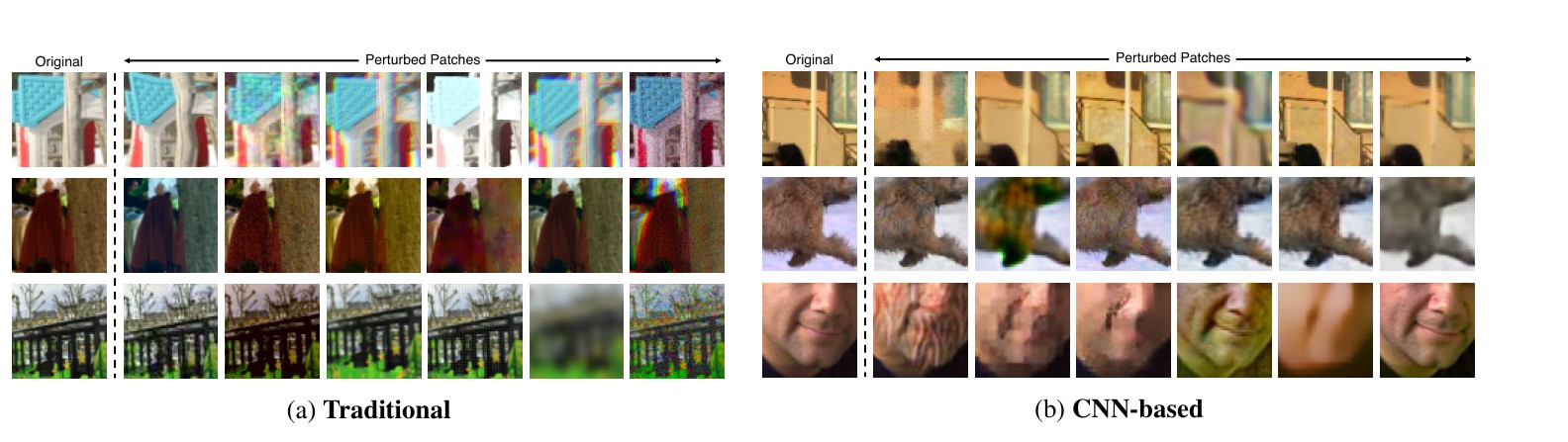
Figure 2: Example distortions. We show example distortions using our (a) traditional and (b) CNN-based methods.
图 2:失真示例。我们展示用(a)传统方法和(b)基于 CNN 的方法得到的失真例子。
Prior work on datasets In order to evaluate existing similarity measures, a number of datasets have been proposed. Some of the most popular are the LIVE [50], TID2008 [45], CSIQ [29], and TID2013 [44] datasets. These datasets are referred to Full-Reference Image Quality Assessment (FR-IQA) datasets and have served as the de-facto baselines for development and evaluation of similarity metrics. A related line of work is on No-Reference Image Quality Assessment (NR-IQA), such as AVA [38] and LIVE In the Wild [18]. These datasets investigate the “quality” of individual images by themselves, without a reference image. We collect a new dataset that is complementary to these: it contains a substantially larger number of distortions, including some from newer, deep network based outputs, as well as geometric distortions. Our dataset is focused on perceptual similarity, rather than quality assessment. Additionally, it is collected on patches as opposed to full images, in the wild, with a different experimental design (more details in Sec 2).
关于数据集的已有工作 为了评估已有的相似度度量,已有若干数据集被提出。其中较常用的包括 LIVE [50]、TID2008 [45]、CSIQ [29] 和 TID2013 [44]。这些数据集被称为全参考图像质量评价(Full-Reference Image Quality Assessment,FR-IQA)数据集,并已成为开发和评估相似度度量的事实基准。另一条相关工作线是无参考图像质量评价(No-Reference Image Quality Assessment,NR-IQA),例如 AVA [38] 和 LIVE In the Wild [18]。这类数据集考察的是单张图像自身的“质量”,并不提供参考图。我们采集的新数据集与它们形成补充:其中的失真种类明显更多,既包括较新的、基于深度网络的输出,也包括几何失真。我们的数据集关注的是感知相似度,而不是质量评价。此外,它采集的是图像块而非整图,在自然环境中进行,实验设计也有所不同(详见第 2 节)。
Prior work on deep networks and human judgments Recently, advances in DNNs have motivated investigation of applications in the context of visual similarity and image quality assessment. Kim and Lee [25] use a CNN to predict visual similarity by training on low-level differences. Concurrent work by Talebi and Milanfar [53, 54] train a deep network in the context of NR-IQA for image aesthetics. Gao et al. [16] and Amirshahi et al. [3] propose techniques involving leveraging internal activations of deep networks (VGG and AlexNet, respectively) along with additional multiscale post-processing. In this work, we conduct a more in-depth study across different architectures, training signals, on a new, large scale, highly-varied dataset.
关于深度网络与人类判断的已有工作 近来,深度神经网络的进展促使人们把它们用到视觉相似度和图像质量评价中。Kim 和 Lee [25] 用 CNN 在低层差异上训练,以预测视觉相似度。与此同时,Talebi 和 Milanfar [53, 54] 在面向图像美学的 NR-IQA 设定下训练深度网络。Gao 等人 [16] 以及 Amirshahi 等人 [3] 分别利用 VGG 和 AlexNet 的内部激活,并辅以额外的多尺度后处理。在本文中,我们在一套新的、大规模且高度多样的数据集上,针对不同架构和训练信号做了更深入的研究。
Recently, Berardino et al. [6] train networks on perceptual similarity, and importantly, assess the ability of deep networks to make predictions on a separate task – predicting most and least perceptually-noticeable directions of distortion. Similarly, we not only assess image patch similarity on parameterized distortions, but also test generalization to real algorithms, as well as generalization to a separate perceptual task – just noticeable differences.
近来,Berardino 等人 [6] 在感知相似度上训练网络,并且——这一点很重要——评估深度网络在另一项任务上的预测能力:预测感知上最明显和最不明显的失真方向。类似地,我们不仅在参数化失真上评估图像块相似度,还测试对真实算法的泛化,以及对另一项感知任务——刚辨差——的泛化。
- Berkeley-Adobe Perceptual Patch Similarity (BAPPS) Dataset
- Berkeley-Adobe 感知图像块相似度(BAPPS)数据集
To evaluate the performance of different perceptual metrics, we collect a large-scale highly diverse dataset of perceptual judgments using two approaches. Our main data collection employs a two alternative forced choice (2AFC) test, that asks which of two distortions is more similar to a reference. This is validated by a second experiment where we perform a just noticeable difference (JND) test, which asks whether two patches – one reference and one distorted – are the same or different. These judgments are collected over a wide space of distortions and real algorithm outputs.
为了评估不同感知度量的表现,我们用两种方式采集了一套大规模、高度多样的感知判断数据集。主要采集采用二项迫选(two alternative forced choice,2AFC)测试,询问两种失真中哪一种与参考更相似。这一做法由第二项实验加以验证:我们进行刚辨差(just noticeable difference,JND)测试,询问两块图像——一块是参考、一块是失真——是相同还是不同。这些判断覆盖了广阔的失真空间以及真实算法输出。
| Dataset | # Input Imgs/Patches | Input Type | Num Distort. | Distort. Types | # Levels | # Distort. Imgs/Patches | # Judgments | Judgment Type |
|---|---|---|---|---|---|---|---|---|
| LIVE [50] | 29 | images | 5 | traditional | continuous | .8k | 25k | MOS |
| CSIQ [29] | 30 | images | 6 | traditional | 5 | .8k | 25k | MOS |
| TID2008 [45] | 25 | images | 17 | traditional | 4 | 2.7k | 250k | MOS |
| TID2013 [44] | 25 | images | 24 | traditional | 5 | 3.0k | 500k | MOS |
| BAPPS (2AFC–Distort) | 160.8k | patch | 425 | trad + CNN | continuous | 321.6k | 349.8k | 2AFC |
| BAPPS (2AFC–Real alg) | 26.9k | patch | – | alg outputs | – | 53.8k | 134.5k | 2AFC |
| BAPPS (JND–Distort) | 9.6k | patch | 425 | trad. + CNN | continuous | 9.6k | 28.8k | Same/Not same |
Table 1: Dataset comparison. A primary differentiator between our proposed Berkeley-Adobe Perceptual Patch Similarity (BAPPS) dataset and previous work is scale of distortion types. We provide human perceptual judgments on distortion set using uncompressed images from [7, 10]. Previous datasets have used a small number of distortions at discrete levels. We use a large number of distortions (created by sequentially composing atomic distortions together) and sample continuously. For each input patch, we corrupt it using two distortions and ask for a few human judgments (2 for train, 5 for test set) per pair. This enables us to obtain judgments on a large number of patches. Previous databases summarize their judgments into a mean opinion score (MOS); we simply report pairwise judgments (two alternative force choice). In addition, we provide judgments on outputs from real algorithms, as well as a same/not same Just Noticeable Difference (JND) perceptual test.
| 数据集 | 输入图像/图像块数 | 输入类型 | 失真数目 | 失真类型 | 等级数 | 失真图像/图像块数 | 判断数 | 判断类型 |
|---|---|---|---|---|---|---|---|---|
| LIVE [50] | 29 | 图像 | 5 | 传统 | 连续 | .8k | 25k | MOS |
| CSIQ [29] | 30 | 图像 | 6 | 传统 | 5 | .8k | 25k | MOS |
| TID2008 [45] | 25 | 图像 | 17 | 传统 | 4 | 2.7k | 250k | MOS |
| TID2013 [44] | 25 | 图像 | 24 | 传统 | 5 | 3.0k | 500k | MOS |
| BAPPS(2AFC–失真) | 160.8k | 图像块 | 425 | 传统 + CNN | 连续 | 321.6k | 349.8k | 2AFC |
| BAPPS(2AFC–真实算法) | 26.9k | 图像块 | – | 算法输出 | – | 53.8k | 134.5k | 2AFC |
| BAPPS(JND–失真) | 9.6k | 图像块 | 425 | 传统 + CNN | 连续 | 9.6k | 28.8k | 相同/不同 |
表 1:数据集比较。我们提出的 Berkeley-Adobe 感知图像块相似度(Berkeley-Adobe Perceptual Patch Similarity,BAPPS)数据集与以往工作的一个主要区别,在于失真类型的规模。我们在来自 [7, 10] 的未压缩图像上,为失真集合提供人类感知判断。以往数据集只用较少的失真,并且取离散等级。我们使用大量失真(把原子失真顺序组合起来生成),并做连续采样。对每个输入图像块,我们用两种失真加以破坏,并就每一对询问少量人类判断(训练集 2 次,测试集 5 次)。这样就能在大量图像块上得到判断。以往数据库把判断汇总成平均意见分(mean opinion score,MOS);我们则直接报告成对判断(二项迫选)。此外,我们还提供真实算法输出上的判断,以及相同/不同的刚辨差(JND)感知测试。
2.1. Distortions
2.1. 失真
Traditional distortions We create a set of “traditional” distortions consisting of common operations performed on the input patches, listed in Table 2 (left). In general, we use photometric distortions, random noise, blurring, spatial shifts and corruptions, and compression artifacts. We show qualitative examples of our traditional distortions in Figure 2. The severity of each perturbation is parameterized – for example, for Gaussian blur, the kernel width determines the amount of corruption applied to the input image. We also compose pairs of distortions sequentially to increase the overall space of possible distortions. In total, we have 20 distortions and 308 sequentially composed distortions.
传统失真 我们构造了一组“传统”失真,由对输入图像块常做的操作组成,列于表 2(左)。总体上,我们使用光度失真、随机噪声、模糊、空间平移与破坏,以及压缩伪影。图 2 给出了传统失真的定性示例。每种扰动的强度都加以参数化——例如对高斯模糊,核宽度决定施加到输入图像上的破坏程度。我们还会把成对的失真顺序组合,以扩大可能失真的总体空间。合计有 20 种失真,以及 308 种顺序组合失真。
CNN-based distortions To more closely simulate the space of artifacts that can arise from deep-learning based methods, we create a set of distortions created by neural networks. We simulate possible algorithm outputs by exploring a variety of tasks, architectures, and losses, as shown in Table 2 (right). Such tasks include autoencoding, denoising, colorization, and superresolution. All of these tasks can be achieved by applying the appropriate corruption to the input. In total, we generated 96 “denoising autoencoders” and use these as CNN-based distortion functions. We train each of these networks on the 1.3M ImageNet dataset [46] for 1 epoch. The goal of each network is not to solve the task per se, but rather to explore common artifacts that plague the outputs of deep learning based methods.
基于 CNN 的失真 为了更贴近地模拟基于深度学习的方法可能产生的伪影空间,我们构造了一组由神经网络生成的失真。如表 2(右)所示,我们通过探索多种任务、架构和损失,来模拟可能的算法输出。这类任务包括自编码、去噪、上色和超分辨率。它们都可以通过对输入施加相应的破坏来实现。我们总共生成了 96 个“去噪自编码器”,并把它们当作基于 CNN 的失真函数。每个网络都在 130 万张图像的 ImageNet 数据集 [46] 上训练 1 个 epoch。每个网络的目标并不在于真正解决该任务,而是探索基于深度学习的方法输出中常见的伪影。
Traditional distortions (left)
| Sub-type | Distortion type |
|---|---|
| Photometric | lightness shift, color shift, contrast, saturation |
| Noise | uniform white noise, Gaussian white, pink, & blue noise, Gaussian colored (between violet and brown) noise, checkerboard artifact |
| Blur | Gaussian, bilateral filtering |
| Spatial | shifting, affine warp, homography, linear warping, cubic warping, ghosting, chromatic aberration, |
| Compression | jpeg |
CNN-based distortions (right)
| Parameter type | Parameters |
|---|---|
| Input corruption | null, pink noise, white noise, color removal, downsampling |
| Generator network architecture | # layers, # skip connections, # layers with dropout, force skip connection at highest layer, upsampling method, normalization method, first layer stride, # channels in layer, max # channels |
| Discriminator | number of layers |
| Loss/Learning | weighting on oixel-wise (), VGG, discriminator losses, learning rate |
Table 2: Our distortions. Our traditional distortions (left) are performed by basic low-level image editing operations. We also sequentially compose them to better explore the space. Our CNN-based distortions (right) are formed by randomly varying parameters such as task, network architecture, and learning parameters. The goal of the distortions is to mimic plausible distortions seen in real algorithm outputs.
传统失真(左)
| 子类 | 失真类型 |
|---|---|
| 光度 | 亮度偏移、颜色偏移、对比度、饱和度 |
| 噪声 | 均匀白噪声,高斯白、粉及蓝噪声,高斯有色(介于紫与棕之间)噪声,棋盘伪影 |
| 模糊 | 高斯、双边滤波 |
| 空间 | 平移、仿射扭曲、单应变换、线性扭曲、三次扭曲、重影、色差, |
| 压缩 | jpeg |
基于 CNN 的失真(右)
| 参数类型 | 参数 |
|---|---|
| 输入破坏 | 无、粉噪声、白噪声、去色、下采样 |
| 生成器网络架构 | 层数、跳跃连接数、带 dropout 的层数、是否在最高层强制跳跃连接、上采样方法、归一化方法、第一层步长、第 1 层通道数、最大通道数 |
| 判别器 | 层数 |
| 损失/学习 | 逐像素()、VGG、判别器损失的权重,学习率 |
表 2:我们的失真。传统失真(左)由基本的低层图像编辑操作完成。我们还会把它们顺序组合,以便更好地探索该空间。基于 CNN 的失真(右)则通过随机改变任务、网络架构和学习参数等形成。这些失真的目标,是模仿真实算法输出中可能出现的失真。
Distorted image patches from real algorithms The true test of an image assessment algorithm is on real problems and real algorithms. We gather perceptual judgments using such outputs. Data on real algorithms is more limited, as each application will have their own unique properties. For example, different colorization methods will not show much structural variation, but will be prone to effects such as color bleeding and color variation. On the other hand, superresolution will not have color ambiguity, but may see larger structural changes from algorithm to algorithm.
来自真实算法的失真图像块 图像评价算法的真正考验,是在真实问题和真实算法上。我们用这类输出收集感知判断。关于真实算法的数据更有限,因为每种应用都有自己独特的性质。例如,不同的上色方法在结构上不会有太大变化,但容易出现颜色溢出和颜色波动等效应。另一方面,超分辨率不会有颜色上的含混,但算法与算法之间可能会看到更大的结构变化。
Superresolution We evaluate results from the 2017 NTIRE workshop [2]. We use 3 tracks from the workshop – , , upsampling rates using “unknown” downsampling to create the input images. Each track had approximately 20 algorithm submissions. We also evaluate several additional methods, including bicubic upsampling, and four of the top performing deep superresolution methods [24, 58, 31, 47]. A common qualitative way of presenting superresolution results is zooming into specific patches and comparing differences. As such, we sample random triplets from random locations of images in the Div2K [2] dataset – the ground truth high-resolution image, along with two algorithm outputs.
超分辨率 我们评估 2017 年 NTIRE 研讨会 [2] 的结果。我们使用该研讨会的 3 个赛道——以“未知”下采样生成输入图像,上采样倍率分别为 、、。每个赛道大约有 20 个算法提交。我们还评估了若干额外方法,包括双三次上采样,以及四种表现居前的深度超分辨率方法 [24, 58, 31, 47]。展示超分辨率结果的一种常用定性方式,是放大到特定图像块并比较差异。因此,我们从 Div2K [2] 数据集图像的随机位置采样随机的 三元组:真实高分辨率图像,以及两个算法输出。
Frame interpolation We sample patches from different frame interpolation algorithms, including three variants of flow-based interpolation [33], CNN-based interpolation [39], and phase-based interpolation [37] on the Davis Middleburry dataset [49]. Because artifacts arising from frame interpolation may occur at different scales, we randomly rescale the image before sampling a patch triplet.
帧插值 我们从不同的帧插值算法中采样图像块,包括基于光流的插值的三种变体 [33]、基于 CNN 的插值 [39],以及在 Davis Middleburry 数据集 [49] 上的基于相位的插值 [37]。由于帧插值产生的伪影可能出现在不同尺度,我们在采样图像块三元组之前会随机缩放图像。
Video deblurring We sample from the video deblurring dataset [52], along with deblurring outputs from Photoshop Shake Reduction, Weighted Fourier Aggregation [11], and three variants of a deep video deblurring method [52].
视频去模糊 我们从视频去模糊数据集 [52] 中采样,同时包括 Photoshop 防抖(Shake Reduction)、加权傅里叶聚合 [11],以及一种深度视频去模糊方法的三种变体 [52] 的去模糊输出。
Colorization We sample patches using random scales on the colorization task, on images from the ImageNet dataset [46]. The algorithms are from pix2pix [22], Larsson et al. [30], and variants from Zhang et al. [62].
上色 我们在上色任务上按随机尺度采样图像块,图像来自 ImageNet 数据集 [46]。算法来自 pix2pix [22]、Larsson 等人 [30],以及 Zhang 等人 [62] 的变体。
2.2. Psychophysical Similarity Measurements
2.2. 心理物理相似度测量
2AFC similarity judgments We randomly select an image patch and apply two distortions to produce patches , . We then ask a human which is closer to the original patch , and record response . On average, people spent approximately 3 seconds per judgment. Let denote our dataset of patch triplets .
2AFC 相似度判断 我们随机选取一个图像块 ,并施加两种失真,得到图像块 、。然后询问人类哪一块更接近原始图像块 ,并记录回答 。平均而言,每次判断大约花费 3 秒。记 为我们的图像块三元组数据集 。
A comparison between our dataset and previous datasets is shown in Table 1. Previous datasets have focused on collecting large numbers of human judgments for a few images and distortion types. For example, the largest dataset, TID2013 [44], has 500k judgments on 3000 distortions (from 25 input images with 24 distortions types, each sampled at 5 levels). We provide a complementary dataset that focuses instead on a large number of distortions types. In, addition, we collect judgments on a large number of patches rather than a small number of images. There are three reasons for this. First, the space of full images is extremely large, which makes it much harder to cover a reasonable portion of the domain with judgments (even color patches represent an intractable 12k-dimensional space). Second, by choosing a smaller patch size, we focus on lower-level aspects of similarity, to mitigate the effect of differing “respects of similarity” that may be influenced by high-level semantics [36]. Finally, modern methods for image synthesis train deep networks with patch-based losses (implemented as convolutions) [8, 21]. Our dataset consists of over 161k patches, derived from the MIT-Adobe 5k dataset [7] (5000 uncompressed images) for training, and the RAISE1k dataset [10] for validation.
我们的数据集与以往数据集的比较见表 1。以往数据集的重点,是在少量图像和失真类型上收集大量人类判断。例如规模最大的 TID2013 [44],在 3000 种失真上有 50 万次判断(来自 25 张输入图像、24 种失真类型,每种在 5 个等级上采样)。我们提供的是一套互补的数据集,转而关注大量失真类型。此外,我们是在大量 图像块上收集判断,而不是在少量整图上。这样做有三个原因。第一,整图空间极大,要用判断覆盖其中合理的一部分困难得多(即便 的彩色图像块,也已是难以处理的 1.2 万维空间)。第二,选用较小的图像块,可以把重点放在相似度的较低层方面,以减轻可能受高层语义影响的不同“相似方面”的作用 [36]。最后,现代图像合成方法用基于图像块的损失(以卷积实现)来训练深度网络 [8, 21]。我们的数据集包含超过 16.1 万个图像块,训练来自 MIT-Adobe 5k 数据集 [7](5000 张未压缩图像),验证来自 RAISE1k 数据集 [10]。
To enable large-scale collection, our data is collected “in-the-wild” on Amazon Mechanical Turk, as opposed to a controlled lab setting. Crump et al. [9] show that AMT can be reliably used to replicate many psychophysics studies, despite the inability to control all environmental factors. We ask for 2 judgments per example in our “train” set and 5 judgments in our “val” sets. Asking for fewer judgments enables us to explore a larger set of image patches and distortions. We add sentinels which consist of pairs of patches with obvious deformations, e.g., a large amount of Gaussian noise vs a small amount of Gaussian noise. Approximately 90% of Turkers were able to correctly pass at least 93% of the sentinels (14 of 15), indicating that they understood the task and were paying attention. We choose to use a larger number of distortions than prior datasets
为了实现大规模采集,我们的数据是在 Amazon Mechanical Turk 上“野外”收集的,而不是在受控的实验室环境中。Crump 等人 [9] 表明,尽管无法控制全部环境因素,AMT 仍可可靠地复现许多心理物理学研究。我们在“训练”集上每个样本询问 2 次判断,在“验证”集上询问 5 次。减少每次的判断次数,使我们能够探索更多的图像块和失真。我们加入了哨兵样本,由带有明显变形的成对图像块组成,例如大量高斯噪声对少量高斯噪声。大约 90% 的众包工人能够正确通过至少 93% 的哨兵(15 题中的 14 题),说明他们理解了任务并且保持了注意。我们选择使用比以往数据集更多的失真
Just noticeable differences (JND) A potential shortcoming of the 2AFC task is that it is “cognitively penetrable,” in the sense that participants can consciously choose which respects of similarity they will choose to focus on in completing the task [36], which introduces subjectivity into the judgments. To validate that the judgments actually reflected something objective and meaningful, we also collected user judgments of “just noticeable differences” (JNDs). We show a reference image, followed by a randomly distorted image, and ask a human if the images are the same or different. The two image patches are shown for 1 second each, with a 250 ms gap in between. Two images which look similar may be easily confused, and a good perceptual metric will be able to order pairs from most to least confusable. JND tests like this may be considered less subjective, since there is a single correct answer for each judgment, and participants are presumed to be aware of what correct behavior entails. We gather 3 JND observations for each of the 4.8k patches in our traditional and CNN-based validation sets. Each subject is shown 160 pairs, along with 40 sentinels (32 identical and 8 with large Gaussian noise distortion applied). We also provide a short training period of 10 pairs which contain 4 “same” pairs, 1 obviously different pair, and 5 “different” pairs generated by our distortions.
刚辨差(JND) 2AFC 任务的一个潜在不足是它“可被认知穿透”:参与者可以有意识地选择在完成任务时把注意放在哪一种相似方面上 [36],从而把主观性带进判断。为验证这些判断确实反映了某种客观而有意义的东西,我们还收集了用户关于“刚辨差”(JND)的判断。我们先出示一张参考图,再出示一张随机失真的图,并询问人类这两张图是相同还是不同。两块图像各显示 1 秒,中间间隔 250 毫秒。看起来相似的两张图可能很容易被混淆,而一种好的感知度量应能把成对样本从最易混淆排到最不易混淆。这类 JND 测试可以被看作不那么主观,因为每次判断都有唯一的正确答案,并且可以假定参与者清楚何谓正确行为。我们在传统和基于 CNN 的验证集中,为 4800 个图像块各收集 3 次 JND 观察。每位被试会看到 160 对,外加 40 个哨兵(32 对完全相同,8 对施加了大幅度高斯噪声失真)。我们还提供一段 10 对的简短训练,其中包含 4 对“相同”、1 对明显不同,以及 5 对由我们的失真生成的“不同”。
| Dataset | Data source | Train/Val | # Examples | # Judge/Example |
|---|---|---|---|---|
| Traditional | [7] | Train | 56.6k | 2 |
| CNN-based | [7] | Train | 38.1k | 2 |
| Mixed | [7] | Train | 56.6k | 2 |
| 2AFC–Distort [Trn] | – | Train | 151.4k | 2 |
| Traditional | [10] | Train | 4.7k | 5 |
| CNN-based | [10] | Train | 4.7k | 5 |
| 2AFC–Distort [Val] | – | Val | 9.4k | 5 |
| Superres | [32] | Val | 10.9k | 5 |
| Frame Interp | [49] | Val | 1.9 | 5 |
| Video Deblur | [5] | Val | 9.4 | 5 |
| Colorization | [46] | Val | 4.7 | 5 |
| 2AFC–Real Alg [Val] | – | Val | 26.9k | 5 |
| Traditional | [10] | Val | 4.8k | 3 |
| CNN-based | [10] | Val | 4.8k | 3 |
| JND–Distort | – | Val | 9.6k | 3 |
Table 3: Our dataset breakdown. We split our 2AFC dataset in to three main portions (1,2) training and test sets with our distortions. Our training and test sets contain patches sampled from the MIT5k [7] and RAISE1k [10] datasets, respectively (3) a test set containing real algorithm outputs, containing patches from a variety of applications. Our JND data is on traditional and CNN-based distortions.
| 数据集 | 数据来源 | 训练/验证 | 样本数 | 每个样本的判断数 |
|---|---|---|---|---|
| 传统 | [7] | 训练 | 56.6k | 2 |
| 基于 CNN | [7] | 训练 | 38.1k | 2 |
| 混合 | [7] | 训练 | 56.6k | 2 |
| 2AFC–失真 [训练] | – | 训练 | 151.4k | 2 |
| 传统 | [10] | 训练 | 4.7k | 5 |
| 基于 CNN | [10] | 训练 | 4.7k | 5 |
| 2AFC–失真 [验证] | – | 验证 | 9.4k | 5 |
| 超分辨率 | [32] | 验证 | 10.9k | 5 |
| 帧插值 | [49] | 验证 | 1.9 | 5 |
| 视频去模糊 | [5] | 验证 | 9.4 | 5 |
| 上色 | [46] | 验证 | 4.7 | 5 |
| 2AFC–真实算法 [验证] | – | 验证 | 26.9k | 5 |
| 传统 | [10] | 验证 | 4.8k | 3 |
| 基于 CNN | [10] | 验证 | 4.8k | 3 |
| JND–失真 | – | 验证 | 9.6k | 3 |
表 3:我们的数据集构成。我们把 2AFC 数据分成三个主要部分:(1、2)带有我们失真的训练集和测试集。训练集和测试集中的图像块分别采样自 MIT5k [7] 和 RAISE1k [10] 数据集;(3)一个包含真实算法输出的测试集,其中的图像块来自多种应用。我们的 JND 数据针对传统失真和基于 CNN 的失真。
We chose to do this in order to prime the users towards expecting approximately 40% of the patch pairs to be identical. Indeed, 36.4% of the pairs were marked “same” (70.4% of sentinels and 27.9% of test pairs).
我们这样做,是为了让用户预先预期大约 40% 的图像块对是相同的。事实上,36.4% 的配对被标为“相同”(哨兵中的 70.4%,测试对中的 27.9%)。
- Deep Feature Spaces
- 深度特征空间
We evaluate feature distances in different networks. For a given convolutional layer, we compute cosine distance (in the channel dimension) and average across spatial dimensions and layers of the network. We also discuss how to tune an existing network on our data.
我们在不同网络中评估特征距离。对给定的卷积层,我们计算余弦距离(沿通道维),并在空间维和网络各层上取平均。我们也讨论如何在我们的数据上调节已有网络。
Network architectures We evaluate the SqueezeNet [20], AlexNet [28], and VGG [51] architectures. We use 5 conv layers from the VGG network, which has become the de facto standard for image generation tasks [17, 14, 8]. We also compare against the shallower AlexNet network, which may more closely match the architecture of the human visual cortex [60]. We use the conv1-conv5 layers from [27]. Finally, the SqueezeNet architecture was designed to be extremely lightweight (2.8 MB) in size, with similar classification performance to AlexNet. We use the first conv layer and subsequent “fire” modules.
网络架构 我们评估 SqueezeNet [20]、AlexNet [28] 和 VGG [51] 架构。我们使用 VGG 网络中的 5 个卷积层,它已成为图像生成任务的事实标准 [17, 14, 8]。我们也与更浅的 AlexNet 网络相比较,后者可能更接近人类视觉皮层的架构 [60]。我们使用来自 [27] 的 conv1–conv5 层。最后,SqueezeNet 架构被设计得极为轻量(大小为 2.8 MB),分类表现与 AlexNet 相近。我们使用第一个卷积层及其后的 “fire” 模块。
We additionally evaluate self-supervised methods, including puzzle-solving [40], cross-channel prediction [62, 63], learning from video [42], and generative modeling [13]. We use publicly available networks from these and other methods, which use variants of AlexNet [28].
我们还评估自监督方法,包括解拼图 [40]、跨通道预测 [62, 63]、从视频中学习 [42] 以及生成建模 [13]。我们使用这些方法及其他方法公开发布的网络,它们采用的是 AlexNet 的变体 [28]。

Figure 3: Computing distance from a network (Left) To compute a distance between two patches, , , given a network , we first compute deep embeddings, normalize the activations in the channel dimension, scale each channel by vector , and take the distance. We then average across spatial dimension and across all layers. (Right) A small network is trained to predict perceptual judgment from distance pair .
图 3:由网络计算距离。(左)给定网络 ,要计算两块图像 、 之间的距离 ,我们先计算深度嵌入,在通道维上归一化激活,用向量 缩放各通道,再取 距离。然后在空间维和所有层上取平均。(右)训练一个小网络 ,由距离对 预测感知判断 。
Network activations to distance Figure 3 (left) and Equation 1 illustrate how we obtain the distance between reference and distorted patches , with network . We extract feature stack from layers and unit-normalize in the channel dimension, which we designate as , for layer . We scale the activations channel-wise by vector and compute the distance. Finally, we average spatially and sum channel-wise. Note that using is equivalent to computing cosine distance.
由网络激活得到距离 图 3(左)和公式 1 说明了我们如何用网络 得到参考图像块与失真图像块 、 之间的距离。我们从 层提取特征栈,并在通道维上做单位归一化,记为第 层的 、。再用向量 按通道缩放激活,并计算 距离。最后在空间上取平均,并沿通道求和。注意,取 等价于计算余弦距离。
Training on our data We consider a few variants for training with our perceptual judgments: lin, tune, and scratch. For the lin configuration, we keep pre-trained network weights fixed, and learn linear weights on top. This constitutes a “perceptual calibration” of a few parameters in an existing feature space. For example, for the VGG network, 1472 parameters are learned. For the tune configuration, we initialize from a pre-trained classification model, and allow all the weights for network to be fine-tuned. Finally, for scratch, we initialize the network from random Gaussian weights and train it entirely on our judgments. Overall, we refer to these as variants of our proposed Learned Perceptual Image Patch Similarity (LPIPS) metric. We illustrate the training loss function in Figure 3 (right) and describe it further in the appendix.
在我们的数据上训练 我们考虑几种用感知判断来训练的变体:lin、tune 和 scratch。在 lin 配置中,我们保持预训练的网络权重 固定,只在其上学习线性权重 。这相当于在已有特征空间里对少量参数做一次“感知校准”。例如对 VGG 网络,要学习的参数有 1472 个。在 tune 配置中,我们从预训练的分类模型初始化,并允许网络 的全部权重进行微调。最后,在 scratch 中,我们用随机高斯权重初始化网络,并完全在我们的判断上训练。总的来说,我们把这些称作所提出的学习感知图像块相似度(Learned Perceptual Image Patch Similarity,LPIPS)度量的几种变体。训练损失函数见图 3(右),并在附录中进一步说明。
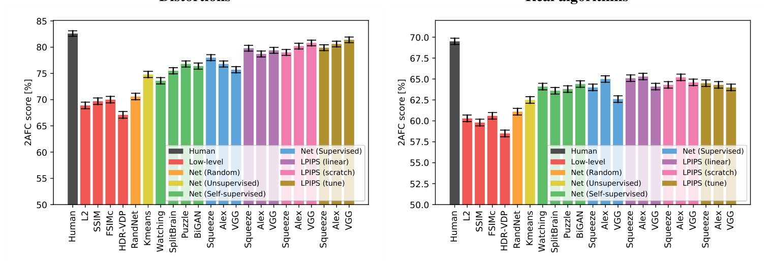
Figure 4: Quantitative comparison. We show a quantitative comparison across metrics on our test sets. (Left) Results averaged across our traditional and CNN-based distortions. (Right) Results averaged across our 4 real algorithm sets.
图 4:定量比较。我们在测试集上对各度量做定量比较。(左)在传统失真和基于 CNN 的失真上平均的结果。(右)在 4 组真实算法集合上平均的结果。
- Experiments
- 实验
Results on our validation sets are shown in Figure 4. We first evaluate how well our metrics and networks work. All validation sets contain 5 pairwise judgments for each triplet. Because this is an inherently noisy process, we compute agreement of an algorithm with all of the judgments. For example, if there are 4 preferences for and 1 for , an algorithm which predicts the more popular choice would receive 80% credit. If a given example is scored with fraction humans in one direction and in the other, a human would achieve score on expectation.
验证集上的结果见图 4。我们首先评估这些度量和网络的表现如何。所有验证集中,每个三元组都有 5 次成对判断。由于这本身是一个有噪声的过程,我们计算算法与全部判断的一致程度。例如,若有 4 次偏好 、1 次偏好 ,则预测更受欢迎选项 的算法会得到 80% 的分数。若某个样本上有比例为 的人朝一个方向、比例为 的人朝另一个方向,则一名人类在期望上会得到 的分数。
4.1. Evaluations
4.1. 评估
How well do low-level metrics and classification networks perform?
低层度量和分类网络的表现如何?
Figure 4 shows the performance of various low-level metrics (in red), deep networks, and human ceiling (in black). The scores are averaged across the 2 distortion test sets (traditional+CNN-based) in Figure 4 (left), and 4 real algorithm benchmarks (superresolution, frame interpolation, video deblurring, colorization) in Figure 4 (right). All scores within each test set are shown in the appendix. Averaged across all 6 test sets, humans are 73.9% consistent. Interestingly, the supervised networks perform at about the same level to each other, at 68.6%, 68.9%, and 67.0%, even across variation in model sizes – SqueezeNet (2.8 MB), AlexNet (9.1 MB), and VGG (58.9 MB) (only convolutional layers are counted). They all perform better than traditional metrics , SSIM, and FSIM at 63.2%, 63.1%, 63.8%, respectively. Despite its common use, SSIM was not designed for situations where geometric distortion is a large factor [48].
图 4 给出了各种低层度量(红色)、深度网络以及人类上限(黑色)的表现。分数在图 4(左)中对 2 个失真测试集(传统 + 基于 CNN)取平均,在图 4(右)中对 4 个真实算法基准(超分辨率、帧插值、视频去模糊、上色)取平均。各测试集内部的全部分数见附录。在全部 6 个测试集上平均,人类的一致性为 73.9%。有趣的是,监督网络彼此表现大致相当,分别为 68.6%、68.9% 和 67.0%,尽管模型大小不同——SqueezeNet(2.8 MB)、AlexNet(9.1 MB)和 VGG(58.9 MB)(只计卷积层)。它们都好于传统度量 、SSIM 和 FSIM,后三者分别为 63.2%、63.1%、63.8%。尽管 SSIM 常用,它并不是为几何失真起重要作用的情形而设计的 [48]。
Does the network have to be trained on classification?
网络必须在分类上训练吗?
In Figure 4, we show model performance across a variety of unsupervised and self-supervised tasks, shown in green – generative modeling with BiGANs [13], solving puzzles [40], cross-channel prediction [63], and segmenting foreground objects from video [42]. These self-supervised tasks perform on par with classification networks. This indicates that tasks across a large spectrum can induce representations which transfer well to perceptual distances. Also, the performance of the stacked -means method [26], shown in yellow, outperforms low-level metrics. Random networks, shown in orange, with weights drawn from a Gaussian, do not yield much improvement. This indicates that the combination of network structure, along with orienting filters in directions where data is more dense, can better correlate to perceptual judgments.
在图 4 中,我们给出多种无监督和自监督任务上的模型表现,以绿色标出——用 BiGAN 做生成建模 [13]、解拼图 [40]、跨通道预测 [63],以及从视频中分割前景物体 [42]。这些自监督任务的表现与分类网络相当。这表明,范围很广的一类任务都能诱导出可较好迁移到感知距离上的表示。此外,以黄色标出的堆叠 -means 方法 [26] 也超过了低层度量。以橙色标出的随机网络(权重从高斯分布中抽取)则没有带来多少提升。这说明,网络结构再加上把滤波器定向到数据更密集的方向,二者结合起来可以与感知判断更好地相关。
In Table 5, we explore how well our perceptual task correlates to semantic tasks on the PASCAL dataset [15], using results summarized in [63], including additional self-supervised methods [1, 43, 12, 56, 62, 41]. We compute the correlation coefficient between each task (perceptual or semantic) across different methods. The correlation from our 2AFC distortion preference task to classification and detection is .640 and .363, respectively. Interestingly, this is similar to the correlation between the classification and detection tasks (.429), even though both are considered “high-level” semantic tasks, and our perceptual task is “low-level.”
在表 5 中,我们考察感知任务与 PASCAL 数据集 [15] 上语义任务的相关程度,所用结果汇总于 [63],其中还包括额外的自监督方法 [1, 43, 12, 56, 62, 41]。我们计算不同方法在各项任务(感知或语义)之间的相关系数。我们的 2AFC 失真偏好任务与分类、检测的相关分别是 .640 和 .363。有趣的是,这与分类和检测这两项任务之间的相关(.429)相近,尽管后两者都被视为“高层”语义任务,而我们的感知任务是“低层”的。
| 2AFC | JND | Class. | Det. | Avg | ||
|---|---|---|---|---|---|---|
| Perceptual | 2AFC | – | .928 | .640 | .363 | .644 |
| Perceptual | JND | .928 | – | .612 | .232 | .591 |
| PASCAL | Classification | .640 | .612 | – | .429 | .560 |
| PASCAL | Detection | .363 | .232 | .429 | – | .341 |
Table 4: Task correlation. We correlate scores between our low-level perceptual tests along with high-level semantic tests across methods. Perceptual scores are averaged between traditional and CNN-based distortion sets. Correlation scores are computed for AlexNet-like architectures.
| 2AFC | JND | 分类 | 检测 | 平均 | ||
|---|---|---|---|---|---|---|
| 感知 | 2AFC | – | .928 | .640 | .363 | .644 |
| 感知 | JND | .928 | – | .612 | .232 | .591 |
| PASCAL | 分类 | .640 | .612 | – | .429 | .560 |
| PASCAL | 检测 | .363 | .232 | .429 | – | .341 |
表 4:任务相关性。我们在不同方法之间,把低层感知测试的分数与高层语义测试的分数做相关。感知分数在传统失真集和基于 CNN 的失真集上取平均。相关系数针对类 AlexNet 的架构计算。
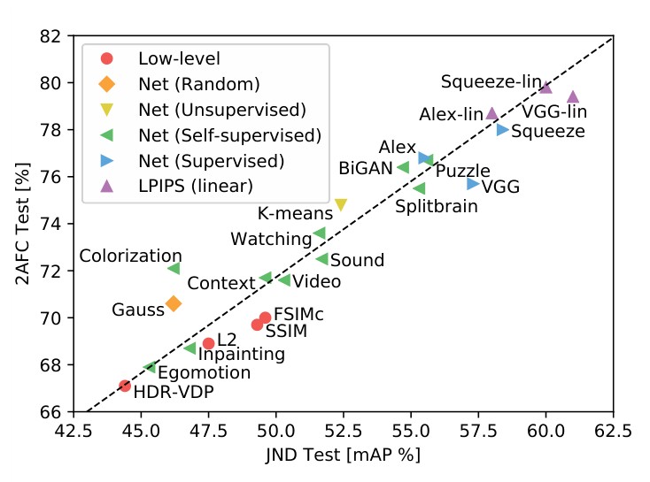
Figure 5: Correlating Perceptual Tests. We show performance across methods, including unsupervised [26], self-supervised [1, 43, 12, 56, 62, 41, 42, 40, 13, 63], supervised [27, 51, 20], and our perceptually-learned metrics (LPIPS). The scores are on our 2AFC and JND tests, averaged across traditional and CNN-based distortions.
图 5:感知测试之间的相关。我们给出各方法的表现,包括无监督 [26]、自监督 [1, 43, 12, 56, 62, 41, 42, 40, 13, 63]、监督 [27, 51, 20],以及我们经感知学习得到的度量(LPIPS)。分数来自我们的 2AFC 和 JND 测试,并在传统失真和基于 CNN 的失真上取平均。
Do metrics correlate across different perceptual tasks?
度量在不同感知任务之间是否相关?
We test if training for the 2AFC distortion preference test corresponds with another perceptual task, the JND test. We order patch pairs by ascending order by a given metric, and compute precision-recall on our CNN-based distortions – for a good metric, patches which are close together are more likely to be confused for being the same. We compute area under the curve, known as mAP [15]. The 2AFC distortion preference test has high correlation to JND: when averaging the results across distortion types. Figure 5 shows how different methods perform under each perceptual test. This indicates that 2AFC generalizes to another perceptual test and is giving us signal regarding human judgments.
我们测试:为 2AFC 失真偏好测试而做的训练,是否对应于另一项感知任务,即 JND 测试。我们按给定度量把图像块对按升序排列,并在基于 CNN 的失真上计算精确率-召回率——对好的度量而言,靠得更近的图像块更可能被当成相同而混淆。我们计算曲线下面积,即 mAP [15]。2AFC 失真偏好测试与 JND 有很高的相关:在各失真类型上平均时,。图 5 给出了不同方法在各项感知测试下的表现。这表明 2AFC 可以泛化到另一项感知测试,并能为我们提供关于人类判断的信号。
Can we train a metric on traditional and CNN-based distortions?
能否在传统失真和基于 CNN 的失真上训练一种度量?
In Figure 4, we show performance using our lin, scratch, and tune configurations, shown in purple, pink, and brown, respectively. When validating on the traditional and CNN-based distortions (Figure 4(a)), we see improvements. Allowing the network to tune all the way through (brown) achieves higher performance than simply learning linear weights (purple) or training from scratch (pink). The higher capacity network VGG also performs better than the lower capacity SqueezeNet and AlexNet architectures. These results verify that networks can indeed learn from perceptual judgments.
在图 4 中,我们给出 lin、scratch 和 tune 三种配置的表现,分别以紫色、粉色和棕色标出。在传统失真和基于 CNN 的失真上做验证时(图 4(a)),可以看到提升。允许网络一路微调到底(棕色),比只学习线性权重(紫色)或从零训练(粉色)表现更好。容量更高的 VGG 网络也优于容量较低的 SqueezeNet 和 AlexNet 架构。这些结果证实,网络确实可以从感知判断中学习。
Does training on traditional and CNN-based distortions transfer to real-world scenarios?
在传统失真和基于 CNN 的失真上训练,能否迁移到真实场景?
We are more interested in how performance generalizes to real-world algorithms, shown in Figure 4(b). The SqueezeNet, AlexNet, and VGG architectures start at 64.0%, 65.0%, and 62.6%, respectively. Learning a linear classifier (purple) improves performance for all networks. Across the 3 networks and 4 real-algorithm tasks, 11 of the 12 scores improved, indicating that “calibrating” activations on a pre-existing representation using our data is a safe way to achieve a small boost in performance (1.1%, 0.3%, and 1.5%, respectively). Training a network from scratch (pink) yields slightly lower performance for AlexNet, and slightly higher performance for VGG than linear calibration. However, these still outperform low-level metrics. This indicates that the distortions we have expressed do project onto our test-time tasks of judging real algorithms.
我们更关心表现如何泛化到真实世界的算法,见图 4(b)。SqueezeNet、AlexNet 和 VGG 架构的起点分别是 64.0%、65.0% 和 62.6%。学习一个线性分类器(紫色)对所有网络都有提升。在 3 种网络和 4 项真实算法任务上,12 项分数中有 11 项得到改善,说明用我们的数据在已有表示上“校准”激活,是获得小幅提升的稳妥办法(分别为 1.1%、0.3% 和 1.5%)。从零训练网络(粉色)对 AlexNet 略低于线性校准,对 VGG 则略高于线性校准。不过它们仍然超过低层度量。这表明,我们所刻画的失真,确实投射到了判断真实算法这一测试时任务上。
Interestingly, starting with a pre-trained network and tuning throughout lowers transfer performance. This is an interesting negative result, as training for a low-level perceptual task directly does not necessarily perform as well as transferring a representation trained for the high-level task.
有趣的是,从预训练网络出发并一路微调,反而会降低迁移表现。这是一个有意思的负面结果:直接为低层感知任务做训练,未必比迁移为高层任务训练得到的表示表现更好。
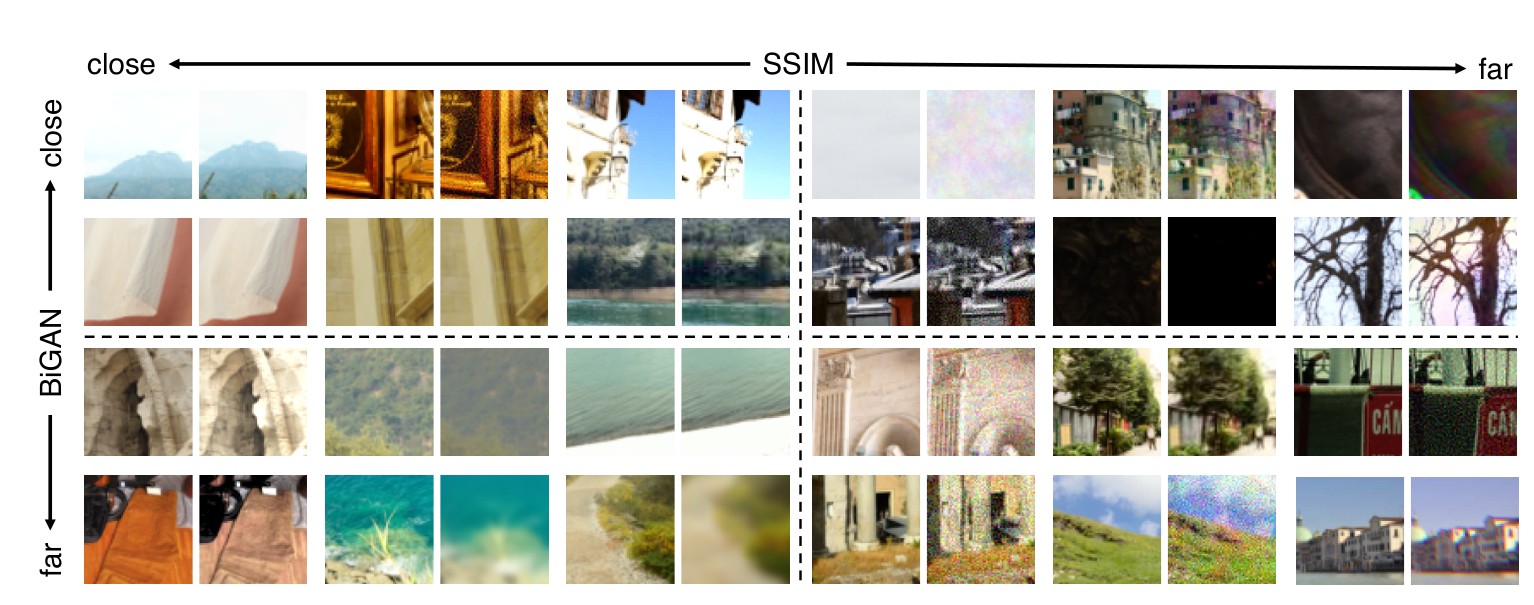
Figure 6: Qualitative comparisons on distortions. We show qualitative comparison on traditional distortions, using the SSIM [57] metric and BiGAN network [13]. We show examples where the metrics agree and siagree. A primary difference is that deep embeddings appear to be more sensitive to blur. Please see the appendix for additional examples.
图 6:失真上的定性比较。我们在传统失真上做定性比较,使用的是 SSIM [57] 度量和 BiGAN 网络 [13]。我们展示度量一致和不一致的例子。一个主要差别是,深度嵌入对模糊似乎更敏感。更多例子见附录。
Where do deep metrics and low-level metrics disagree?
深度度量与低层度量在何处不一致?
In Figure 6, we show a qualitative comparison across our traditional distortions for a deep method, BiGANs [13], and a representation traditional perceptual method, SSIM [57]. Pairs which BiGAN perceives to be far but SSIM to be close generally contain some blur. BiGAN tends to perceive correlated noise patterns to be a smaller distortion than SSIM.
在图 6 中,我们针对一种深度方法 BiGAN [13] 和一种有代表性的传统感知方法 SSIM [57],在传统失真上做定性比较。BiGAN 觉得远、而 SSIM 觉得近的配对,通常含有一定模糊。与 SSIM 相比,BiGAN 往往把相关噪声模式看成较小的失真。
- Conclusions
- 结论
Our results indicate that networks trained to solve challenging visual prediction and modeling tasks end up learning a representation of the world that correlates well with perceptual judgments. A similar story has recently emerged in the representation learning literature: networks trained on self-supervised and unsupervised objectives end up learning a representation that is also effective at semantic tasks [12]. Interestingly, recent findings in neuroscience make much the same point: representations trained on computer vision tasks also end up being effective models of neural activity in macaque visual cortex [60]. Moreover (and roughly speaking), the stronger the representation is at the computer vision task, the stronger it is as a model of cortical activity. Our paper makes a similar finding: the stronger a feature set is at classification and detection, the stronger it is as a model of perceptual similarity judgments, as suggested in Table 4. Together, these results suggest that a good feature is a good feature. Features that are good at semantic tasks are also good at self-supervised and unsupervised tasks, and also provide good models of both human perceptual behavior and macaque neural activity. This last point aligns with the “rational analysis” explanation of visual cognition [4], suggesting that the idiosyncrasies of biological perception arise as a consequence of a rational agent attempting to solve natural tasks. Further refining the degree to which this is true is an important question for future research.
我们的结果表明,为解决有挑战性的视觉预测与建模任务而训练的网络,最终会学到一种与感知判断良好相关的世界表示。表示学习文献中近来也出现了类似的情形:在自监督和无监督目标上训练的网络,最终会学到一种在语义任务上同样有效的表示 [12]。有趣的是,神经科学的近期发现几乎说的是同一件事:在计算机视觉任务上训练的表示,最终也成为猕猴视觉皮层神经活动的有效模型 [60]。而且(大致说来),表示在计算机视觉任务上越强,它作为皮层活动模型也越强。本文得到了类似的发现:一套特征在分类和检测上越强,它作为感知相似度判断的模型也越强,如表 4 所示。合在一起,这些结果说明:好的特征就是好的特征。擅长语义任务的特征,也擅长自监督和无监督任务,并且也能很好地刻画人类的感知行为和猕猴的神经活动。最后这一点与视觉认知的“理性分析”解释 [4] 相一致,即生物感知的种种特点,产生于一个理性智能体试图解决自然任务。进一步弄清这一点在多大程度上成立,是未来研究的一个重要问题。
Acknowledgements This research was supported, in part, by grants from Berkeley Deep Drive, NSF IIS-1633310, and hardware donations by NVIDIA. We thank members of the Berkeley AI Research Lab and Adobe Research for helpful discussions. We thank Alan Bovik for his insightful comments. We also thank Radu Timofte, Zhaowen Wang, Michael Waechter, Simon Niklaus, and Sergio Guadarrama for help preparing data. RZ is partially supported by an Adobe Research Fellowship and much of this work was done while RZ was an intern at Adobe Research.
致谢 本研究部分得到 Berkeley Deep Drive、NSF IIS-1633310 的资助,以及 NVIDIA 的硬件捐赠。我们感谢 Berkeley AI Research Lab 和 Adobe Research 的成员参与有益的讨论。我们感谢 Alan Bovik 提出的深刻意见。我们还感谢 Radu Timofte、Zhaowen Wang、Michael Waechter、Simon Niklaus 和 Sergio Guadarrama 帮助准备数据。RZ 部分得到 Adobe Research Fellowship 的资助,本研究的相当部分是在 RZ 于 Adobe Research 实习期间完成的。
References
参考文献
[1] P. Agrawal, J. Carreira, and J. Malik. Learning to see by moving. In ICCV, pages 37–45, 2015. 7
[2] E. Agustsson and R. Timofte. Ntire 2017 challenge on single image super-resolution: Dataset and study. In CVPR Workshops, July 2017. 4
[3] S. Ali Amirshahi, M. Pedersen, and S. X. Yu. Image quality assessment by comparing cnn features between images. Electronic Imaging, 2017(12):42–51, 2017. 3
[4] J. R. Anderson. The adaptive character of thought. Psychology Press, 1990. 8
[5] S. Baker, D. Scharstein, J. Lewis, S. Roth, M. J. Black, and R. Szeliski. A database and evaluation methodology for optical flow. IJCV, 2011. 5
[6] A. Berardino, V. Laparra, J. Ballé, and E. Simoncelli. Eigendistortions of hierarchical representations. In NIPS, 2017. 3
[7] V. Bychkovsky, S. Paris, E. Chan, and F. Durand. Learning photographic global tonal adjustment with a database of input / output image pairs. In CVPR, 2011. 3, 5
[8] Q. Chen and V. Koltun. Photographic image synthesis with cascaded refinement networks. ICCV, 2017. 2, 5
[9] M. J. Crump, J. V. McDonnell, and T. M. Gureckis. Evaluating amazon’s mechanical turk as a tool for experimental behavioral research. PloS one, 2013. 5
[10] D.-T. Dang-Nguyen, C. Pasquini, V. Conotter, and G. Boato. Raise: a raw images dataset for digital image forensics. In Proceedings of the 6th ACM Multimedia Systems Conference, pages 219–224. ACM, 2015. 3, 5
[11] M. Delbracio and G. Sapiro. Hand-held video deblurring via efficient fourier aggregation. IEEE Transactions on Computational Imaging, 1(4):270–283, 2015. 4
[12] C. Doersch, A. Gupta, and A. A. Efros. Unsupervised visual representation learning by context prediction. In ICCV, 2015. 7, 8
[13] J. Donahue, P. Krähenbühl, and T. Darrell. Adversarial feature learning. ICLR, 2017. 1, 2, 5, 7, 8
[14] A. Dosovitskiy and T. Brox. Generating images with perceptual similarity metrics based on deep networks. In HIPS, pages 658–666, 2016. 2, 5
[15] M. Everingham, L. Van Gool, C. K. I. Williams, J. Winn, and A. Zisserman. The PASCAL Visual Object Classes Challenge 2007 (VOC2007) Results. http://www.pascal-network.org/challenges/VOC/voc2007/workshop/index.html. 7
[16] F. Gao, Y. Wang, P. Li, M. Tan, J. Yu, and Y. Zhu. Deepsim: Deep similarity for image quality assessment. Neurocomputing, 2017. 3
[17] L. A. Gatys, A. S. Ecker, and M. Bethge. Image style transfer using convolutional neural networks. In CVPR, pages 2414– 2423, 2016. 2, 5
[18] D. Ghadiyaram and A. C. Bovik. Massive online crowdsourced study of subjective and objective picture quality. TIP, 2016. 3
[19] N. Goodman. Seven strictures on similarity. Problems and Projects, 1972. 2
[20] F. N. Iandola, S. Han, M. W. Moskewicz, K. Ashraf, W. J. Dally, and K. Keutzer. Squeezenet: Alexnet-level accuracy with 50x fewer parameters and < 0.5 mb model size. CVPR, 2017. 1, 2, 5, 7
[21] P. Isola, J.-Y. Zhu, T. Zhou, and A. A. Efros. Image-to-image translation with conditional adversarial networks. CVPR, 2017. 5
[22] P. Isola, D. Zoran, D. Krishnan, and E. H. Adelson. Learning visual groups from co-occurrences in space and time. ICCV Workshop, 2016. 4
[23] J. Johnson, A. Alahi, and L. Fei-Fei. Perceptual losses for real-time style transfer and super-resolution. ECCV, 2016. 2
[24] J. Kim, J. Kwon Lee, and K. Mu Lee. Accurate image super-resolution using very deep convolutional networks. In CVPR, pages 1646–1654, 2016. 4
[25] J. Kim and S. Lee. Deep learning of human visual sensitivity in image quality assessment framework. In CVPR, 2017. 3
[26] P. Krähenbühl, C. Doersch, J. Donahue, and T. Darrell. Data-dependent initializations of convolutional neural networks. International Conference on Learning Representations, 2016. 1, 2, 7
[27] A. Krizhevsky. One weird trick for parallelizing convolutional neural networks. arXiv preprint arXiv:1404.5997, 2014. 1, 5, 7
[28] A. Krizhevsky, I. Sutskever, and G. E. Hinton. Imagenet classification with deep convolutional neural networks. In NIPS, 2012. 2, 5, 6
[29] E. C. Larson and D. M. Chandler. Most apparent distortion: full-reference image quality assessment and the role of strategy. Journal of Electronic Imaging, 2010. 3
[30] G. Larsson, M. Maire, and G. Shakhnarovich. Learning representations for automatic colorization. ECCV, 2016. 4
[31] C. Ledig, L. Theis, F. Huszár, J. Caballero, A. Cunningham, A. Acosta, A. Aitken, A. Tejani, J. Totz, Z. Wang, et al. Photo-realistic single image super-resolution using a generative adversarial network. CVPR, 2016. 4
[32] B. Lim, S. Son, H. Kim, S. Nah, and K. M. Lee. Enhanced deep residual networks for single image super-resolution. In CVPR Workshops, 2017. 5
[33] C. Liu et al. Beyond pixels: exploring new representations and applications for motion analysis. PhD thesis, Massachusetts Institute of Technology, 2009. 4
[34] R. Mantiuk, K. J. Kim, A. G. Rempel, and W. Heidrich. Hdrvdp-2: A calibrated visual metric for visibility and quality predictions in all luminance conditions. In ACM Transactions on Graphics (TOG), 2011. 1
[35] A. B. Markman and D. Gentner. Nonintentional similarity processing. The new unconscious, pages 107–137, 2005. 2
[36] D. L. Medin, R. L. Goldstone, and D. Gentner. Respects for similarity. Psychological review, 100(2):254, 1993. 2, 5
[37] S. Meyer, O. Wang, H. Zimmer, M. Grosse, and A. Sorkine-Hornung. Phase-based frame interpolation for video. In CVPR, pages 1410–1418, 2015. 4
[38] N. Murray, L. Marchesotti, and F. Perronnin. Ava: A large-scale database for aesthetic visual analysis. In CVPR, 2012. 3
[39] S. Niklaus, L. Mai, and F. Liu. Video frame interpolation via adaptive separable convolution. In ICCV, 2017. 4
[40] M. Noroozi and P. Favaro. Unsupervised learning of visual representations by solving jigsaw puzzles. ECCV, 2016. 1, 2, 5, 7
[41] A. Owens, P. Isola, J. McDermott, A. Torralba, E. H. Adelson, and W. T. Freeman. Visually indicated sounds. CVPR, 2016. 7
[42] D. Pathak, R. Girshick, P. Dollár, T. Darrell, and B. Hariharan. Learning features by watching objects move. CVPR, 2017. 1, 5, 7
[43] D. Pathak, P. Krähenbühl, J. Donahue, T. Darrell, and A. Efros. Context encoders: Feature learning by inpainting. In CVPR, 2016. 7
[44] N. Ponomarenko, L. Jin, O. Ieremeiev, V. Lukin, K. Egiazarian, J. Astola, B. Vozel, K. Chehdi, M. Carli, F. Battisti, et al. Image database tid2013: Peculiarities, results and perspectives. Signal Processing: Image Communication, 2015. 2, 3, 4
[45] N. Ponomarenko, V. Lukin, A. Zelensky, K. Egiazarian, M. Carli, and F. Battisti. Tid2008-a database for evaluation of full-reference visual quality assessment metrics. Advances of Modern Radioelectronics, 2009. 3
[46] O. Russakovsky, J. Deng, H. Su, J. Krause, S. Satheesh, S. Ma, Z. Huang, A. Karpathy, A. Khosla, M. Bernstein, et al. Imagenet large scale visual recognition challenge. IJCV, 2015. 1, 4, 5
[47] M. S. Sajjadi, B. Schölkopf, and M. Hirsch. Enhancenet: Single image super-resolution through automated texture synthesis. ICCV, 2017. 4
[48] M. P. Sampat, Z. Wang, S. Gupta, A. C. Bovik, and M. K. Markey. Complex wavelet structural similarity: A new image similarity index. TIP, 2009. 2, 7
[49] D. Scharstein and R. Szeliski. A taxonomy and evaluation of dense two-frame stereo correspondence algorithms. IJCV, 2002. 4, 5
[50] H. R. Sheikh, M. F. Sabir, and A. C. Bovik. A statistical evaluation of recent full reference image quality assessment algorithms. TIP, 2006. 3
[51] K. Simonyan and A. Zisserman. Very deep convolutional networks for large-scale image recognition. arXiv, 2014. 1, 2, 5, 7
[52] S. Su, M. Delbracio, J. Wang, G. Sapiro, W. Heidrich, and O. Wang. Deep video deblurring for hand-held cameras. In CVPR, 2017. 4
[53] H. Talebi and P. Milanfar. Learned perceptual image enhancement. ICCP, 2018. 3
[54] H. Talebi and P. Milanfar. Nima: Neural image assessment. TIP, 2018. 3
[55] A. Tversky. Features of similarity. Psychological review, 1977. 2
[56] X. Wang and A. Gupta. Unsupervised learning of visual representations using videos. In ICCV, 2015. 7
[57] Z. Wang, A. C. Bovik, H. R. Sheikh, and E. P. Simoncelli. Image quality assessment: from error visibility to structural similarity. TIP, 2004. 1, 2, 8
[58] Z. Wang, D. Liu, J. Yang, W. Han, and T. Huang. Deep networks for image super-resolution with sparse prior. In ICCV, 2015. 4
[59] Z. Wang, E. P. Simoncelli, and A. C. Bovik. Multiscale structural similarity for image quality assessment. In Signals, Systems and Computers. IEEE, 2004. 1
[60] D. L. Yamins and J. J. DiCarlo. Using goal-driven deep learning models to understand sensory cortex. Nature neuroscience, 2016. 5, 8
[61] L. Zhang, L. Zhang, X. Mou, and D. Zhang. Fsim: A feature similarity index for image quality assessment. TIP, 2011. 1, 2
[62] R. Zhang, P. Isola, and A. A. Efros. Colorful image colorization. ECCV, 2016. 4, 5, 7
[63] R. Zhang, P. Isola, and A. A. Efros. Split-brain autoencoders: Unsupervised learning by cross-channel prediction. In CVPR, 2017. 1, 2, 5, 7