LPCNet: Improving Neural Speech Synthesis Through Linear Prediction

LPCNet：用线性预测改进神经语音合成

Jean-Marc Valin Affiliation: Mozilla Affiliation: Mountain View, CA, USA Email: jmvalin@jmvalin.ca    Jan Skoglund Affiliation: Google LLC Affiliation: San Francisco, CA, USA Email: jks@google.com

Abstract

摘要

Neural speech synthesis models have recently demonstrated the ability to synthesize high quality speech for text-to-speech and compression applications. These new models often require powerful GPUs to achieve real-time operation, so being able to reduce their complexity would open the way for many new applications. We propose LPCNet, a WaveRNN variant that combines linear prediction with recurrent neural networks to significantly improve the efficiency of speech synthesis. We demonstrate that LPCNet can achieve significantly higher quality than WaveRNN for the same network size and that high quality LPCNet speech synthesis is achievable with a complexity under 3 GFLOPS. This makes it easier to deploy neural synthesis applications on lower-power devices, such as embedded systems and mobile phones.

神经语音合成模型近来已能在文本到语音与压缩场景中合成高质量语音。这类新模型往往需要强力 GPU 才能实时运行，若能降低复杂度，将打开许多新应用。我们提出 LPCNet：一种把线性预测与循环神经网络结合的 WaveRNN 变体，显著提高语音合成效率。实验表明，在相同网络规模下 LPCNet 的质量明显高于 WaveRNN，且高质量合成可在 3 GFLOPS 以下实现。这使得神经合成更容易部署到功耗更低的设备，例如嵌入式系统与手机。

1 Introduction

1 引言

Index Terms:

Neural speech synthesis algorithms have recently made it possible to both synthesize high-quality speech [1, 2, 3], and code high quality speech at very low bitrate [4]. The first generation of these algorithms, often based on algorithms like WaveNet [5], gave promising results in real time with a high-end GPU to provide the tens of billions of floating-point operations per second (GFLOPS) required. We want to perform synthesis on end-user devices like mobile phones, which do not have powerful GPUs and have limited battery capacity.

索引词：

神经语音合成算法近来既能合成高质量语音 [1, 2, 3]，也能以极低比特率对高质量语音编码 [4]。第一代算法多基于 WaveNet [5] 一类方法，虽能在高端 GPU 提供每秒数十亿次浮点运算（GFLOPS）时实时给出不错结果，但我们希望在手机等终端上合成：这些设备没有强力 GPU，电池容量也有限。

Recent work [6, 7] has focused on finding more efficient models in order to reduce the complexity of speech synthesis. In this work, we continue in that direction, providing more efficiency improvements and making it easier to synthesize speech even on slower CPUs, and with limited impact on battery life.

近期工作 [6, 7] 致力于寻找更高效的模型以降低语音合成复杂度。本文沿同一方向继续推进，进一步提升效率，使较慢 CPU 也能合成语音，并对续航影响有限。

Low complexity parametric synthesis models such as low bitrate vocoders have existed for a long time [8, 9], but their quality has always been severely limited. While they are generally efficient at modeling the spectral envelope (vocal tract response) of the speech using linear prediction, no such simple model exists for the excitation. Despite some advances [10, 11, 12], modeling the excitation signal has remained a challenge.

低复杂度参数合成模型（如低比特率声码器）早已存在 [8, 9]，但质量一直严重受限。它们通常能用线性预测高效刻画语音的谱包络（声道响应），激励却没有同样简单的模型。尽管有一些进展 [10, 11, 12]，激励信号建模仍是难题。

In this work, we propose the LPCNet model, which takes the burden of spectral envelope modeling away from a neural synthesis network so that most of its capacity can be used to model a spectrally flat excitation. This makes it possible to match the quality of state-of-the art neural synthesis systems with fewer neurons, significantly reducing the complexity. Starting from the WaveRNN algorithm summarized in Section 2, we make improvements that reduce the model complexity, as detailed in Section 3. In Section 4, we evaluate the quality and complexity of LPCNet in a speaker-independent speech synthesis context based on the proposed model. We conclude in Section 5.

本文提出 LPCNet：把谱包络建模的负担从神经合成网络上卸下，使网络容量主要用于建模谱平坦的激励。这样可用更少神经元达到与前沿神经合成系统相当的质量，显著降低复杂度。我们从第 2 节概述的 WaveRNN 出发，在第 3 节给出降低模型复杂度的改进；第 4 节在说话人无关的语音合成设定下评估 LPCNet 的质量与复杂度；第 5 节作结。

2 WaveRNN

The WaveRNN architecture proposed in [7] takes as input the previous audio sample $s_{t-1}$, along with conditioning parameters $\mathbf{f}$, and generates a discrete probability distribution $P\left(s_{t}\right)$ for the output sample. Although it is proposed as a 16-bit model (split as 8 coarse bits and 8 fine bits), we omit the coarse/fine split in this summary, both for clarity and because we do not use it in this work. The WaveRNN model mainly consists of a gated recurrent unit (GRU) [13], followed by two fully-connected layers, ending in a softmax activation. It is computed as

文献 [7] 提出的 WaveRNN 以先前音频样本 $s_{t-1}$ 与条件参数 $\mathbf{f}$ 为输入，输出样本的离散概率分布 $P\left(s_{t}\right)$。原作是 16 比特模型（8 位粗 + 8 位细），本概述略去粗/细拆分，既为清晰，也因本文未使用。WaveRNN 主体是一个门控循环单元（GRU）[13]，后接两层全连接并以 softmax 结束，计算为

$$\displaystyle\mathbf{x}_{t} \\ \displaystyle=\left[s_{t-1};\mathbf{f}\right] \\ \displaystyle\mathbf{u}_{t} \\ \displaystyle=\sigma\left(\mathbf{W}^{\left(u\right)}\mathbf{h}_{t-1}+\mathbf{U}^{\left(u\right)}\mathbf{x}_{t}\right) \\ \displaystyle\mathbf{r}_{t} \\ \displaystyle=\sigma\left(\mathbf{W}^{\left(r\right)}\mathbf{h}_{t-1}+\mathbf{U}^{\left(r\right)}\mathbf{x}_{t}\right) \\ \displaystyle\widetilde{\mathbf{h}}_{t} \\ \displaystyle=\tanh\left(\mathbf{r}_{t}\circ\left(\mathbf{W}^{\left(h\right)}\mathbf{h}_{t-1}\right)+\mathbf{U}^{\left(h\right)}\mathbf{x}_{t}\right) \\ \displaystyle\mathbf{h}_{t} \\ \displaystyle=\mathbf{u}_{t}\circ\mathbf{h}_{t-1}+\left(1-\mathbf{u}_{t}\right)\circ\widetilde{\mathbf{h}}_{t} \\ \displaystyle P\left(s_{t}\right) \\ \displaystyle=\mathrm{softmax}\left(\mathbf{W}_{2}\ \mathrm{relu}\left(\mathbf{W}_{1}\mathbf{h}_{t}\right)\right)\ , \tag{1}$$

where the $\mathbf{W}^{\left(\cdot\right)}$ and $\mathbf{U}^{\left(\cdot\right)}$ matrices are the GRU weights, $\sigma\left(x\right)=\frac{1}{1+e^{-x}}$ is the sigmoid function, and $\circ$ denotes an element-wise vector multiply. Throughout this paper, biases are omitted for clarity. The synthesized output sample $s_{t}$ is obtained by sampling from the probability distribution $P\left(s_{t}\right)$. As a way of reducing complexity, the matrices used by the GRU can be made sparse and [7] proposes using non-zero blocks of size 4x4 or 16x1 to ensure that vectorization is still possible and efficient.

其中 $\mathbf{W}^{\left(\cdot\right)}$ 与 $\mathbf{U}^{\left(\cdot\right)}$ 为 GRU 权重，$\sigma\left(x\right)=\frac{1}{1+e^{-x}}$ 为 sigmoid，$\circ$ 表示逐元素乘。全文为清晰起见省略偏置。合成输出样本 $s_{t}$ 从分布 $P\left(s_{t}\right)$ 采样得到。为降低复杂度，GRU 所用矩阵可稀疏化；[7] 建议使用 4×4 或 16×1 的非零块，以便仍能高效向量化。

3 LPCNet

This section presents the LPCNet model, our proposed improvement on WaveRNN. Fig. 1 shows an overview of its architecture, which is explained in more details in this section. It includes a sample rate network that operates at 16 kHz, and a frame rate network that processes 10-ms frames (160 samples). In this work, we limit the input of the synthesis to just 20 features: 18 Bark-scale [14] cepstral coefficients, and 2 pitch parameters (period, correlation). For low-bitrate coding applications, the cepstrum and pitch parameters would be quantized [4], whereas for text-to-speech, they would be computed from the text using another neural network [1].

本节介绍我们在 WaveRNN 上提出的改进——LPCNet。图 1 给出架构概览，细节见后文。它包含以 16 kHz 运行的采样率网络，以及处理 10 ms 帧（160 个样本）的帧率网络。本文将合成输入限制为仅 20 维特征：18 个 Bark 尺度 [14] 倒谱系数，以及 2 个基音参数（周期、相关）。低比特率编码场景下，倒谱与基音会量化 [4]；文本到语音场景下，则由另一神经网络从文本算出 [1]。

3.1 Conditioning Parameters

3.1 条件参数

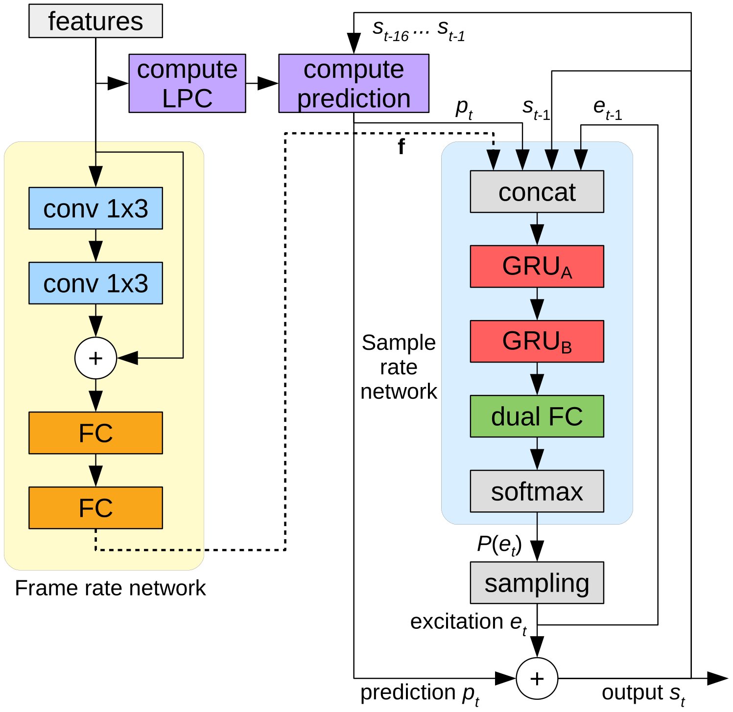
Figure 1: Overview of the LPCNet algorithm. The left part of the network (yellow) is computed once per frame and its result is held constant throughout the frame for the sample rate network on the right (blue). The compute prediction block predicts the sample at time $t$ based on previous samples and on the linear prediction coefficients. Conversions between $\mu$-law and linear are omitted for clarity. The de-emphasis filter is applied to the output $s_{t}$.

图 1：LPCNet 算法概览。网络左侧（黄）每帧计算一次，结果在整帧内对右侧采样率网络（蓝）保持恒定。compute prediction 块根据先前样本与线性预测系数预测时刻 $t$ 的样本。$\mu$-law 与线性之间的转换为清晰起见省略。去加重滤波作用于输出 $s_{t}$。

As part of the frame rate network, the 20 features first go through two convolutional layers with a filter size of 3 (conv 3x1), resulting in a receptive field of 5 frames (two frames ahead and two frames back). The output of the two convolutional layers is added to a residual connection and then goes through two fully-connected layers. The frame rate network outputs a 128-dimensional conditioning vector $\mathbf{f}$ that is then used by the sample rate network. The vector $\mathbf{f}$ is held constant for the duration of each frame.

在帧率网络中，20 维特征先经两层滤波器大小为 3 的卷积（conv 3×1），感受野为 5 帧（前两帧与后两帧）。两层卷积输出与残差相加，再经两层全连接。帧率网络输出 128 维条件向量 $\mathbf{f}$，供采样率网络使用；向量 $\mathbf{f}$ 在每帧持续时间内保持不变。

3.2 Pre-emphasis and Quantization

3.2 预加重与量化

Some synthesis models such as WaveNet [5] use 8-bit $\mu$-law quantization [15] to reduce the number of possible output sample values to just 256. Because the energy of speech signals tends to be mostly concentrated in the low frequencies, the $\mu$-law white quantization noise is often audible in the high frequencies, especially for 16 kHz signals that have a higher spectral tilt. To avoid this problem, some approaches extend the output to 16 bits [7]. Instead, we propose to simply apply a first-order pre-emphasis filter $E(z)=1-\alpha z^{-1}$ to the training data, with $\alpha=0.85$ providing good results. The synthesis output can then be filtered using the inverse (de-empahsis) filter

WaveNet [5] 等合成模型使用 8 比特 $\mu$-law 量化 [15]，把可能输出样本值减到 256 个。语音能量多集中在低频，$\mu$-law 白量化噪声在高频常可闻，对谱倾斜更大的 16 kHz 信号尤甚。有的方法把输出扩到 16 比特以规避 [7]。我们改为对训练数据施加一阶预加重滤波 $E(z)=1-\alpha z^{-1}$，$\alpha=0.85$ 效果良好。合成输出再用逆（去加重）滤波

$$D(z)=\frac{1}{1-\alpha z^{-1}}\ , \tag{2}$$

effectively shaping the noise such that its power at the Nyquist rate is reduced by 16 dB. This significantly reduces the perceived noise (see Section 4.3) and makes 8-bit $\mu$-law output viable for high-quality synthesis.

从而塑造噪声，使奈奎斯特频率处功率降低约 16 dB。这显著减弱可感知噪声（见第 4.3 节），使 8 比特 $\mu$-law 输出可用于高质量合成。

3.3 Linear Prediction

3.3 线性预测

The neural networks in many neural speech synthesis approaches [4, 5, 6, 7, 16] have to model the entire speech production process, including glottal pulses, noise excitation, as well as the response of the vocal tract. Although some of these are indeed very hard to model, we know that the vocal tract response can be represented reasonably well by a simple all-pole linear filter [17]. Let $s_{t}$ be the signal at time $t$, its linear prediction based on previous samples is

许多神经语音合成方法 [4, 5, 6, 7, 16] 中的网络须建模整条发声链路，包括声门脉冲、噪声激励以及声道响应。其中一些确实很难建模，但声道响应可用简单的全极点线性滤波器较好表示 [17]。令 $s_{t}$ 为时刻 $t$ 的信号，基于先前样本的线性预测为

$$p_{t}=\sum_{k=1}^{M}a_{k}s_{t-k}\ , \tag{3}$$

where $a_{k}$ are the $M^{th}$ order linear prediction coefficients (LPC) for the current frame.

其中 $a_{k}$ 为当前帧的 $M$ 阶线性预测系数（LPC）。

The prediction coefficients $a_{k}$ are computed by first converting the 18-band Bark-frequency cepstrum into a linear-frequency power spectral density (PSD). The PSD is then converted to an auto-correlation using an inverse FFT. From the auto-correlation, the Levinson-Durbin algorithm is used to compute the predictor. Computing the predictor from the cepstrum ensures that no additional information needs to be transmitted (in a speech coding context) or synthesized (in a text-to-speech context). Even though the LPC analysis computed in this way is not as accurate as one computed on the input signal (due to the low resolution of the cepstrum), the effect on the output is small because the network is able to learn to compensate. This is an advantage over open-loop filtering approaches [12].

预测系数 $a_{k}$ 的求法是：先把 18 带 Bark 频率倒谱转为线性频率功率谱密度（PSD）；PSD 经逆 FFT 转为自相关；再由 Levinson–Durbin 算法得到预测器。从倒谱算预测器，保证编码时无需额外传输、TTS 时无需额外合成信息。尽管这样得到的 LPC 分析不如在输入信号上直接计算精确（倒谱分辨率低），但对输出影响很小，因为网络能学会补偿。这相对开环滤波方法 [12] 是优势。

As an obvious extension of using a linear predictor to help the neural network, we can also have the network directly predict the excitation (prediction residual) rather than the sample values. This is not only a slightly easier task for the network, but it also slightly reduces the $\mu$-law quantization noise, since the excitation generally has a smaller amplitude than the pre-emphasized signal. The network takes as input the previously sampled excitation $e_{t-1}$, but also the past signal $s_{t-1}$, and the current prediction $p_{t}$. We still include $s_{t-1}$ and $p_{t}$ because we find that open-loop synthesis based only on $e_{t-1}$ produces bad quality speech (see Section 3.8).

用线性预测帮助神经网络的自然延伸，是让网络直接预测激励（预测残差）而非样本值。这对网络稍易，也因激励幅度通常小于预加重信号，可略降 $\mu$-law 量化噪声。网络输入包括先前采样的激励 $e_{t-1}$，以及过去信号 $s_{t-1}$ 与当前预测 $p_{t}$。仍保留 $s_{t-1}$ 与 $p_{t}$，因为我们发现仅基于 $e_{t-1}$ 的开环合成质量很差（见第 3.8 节）。

3.4 Output Layer

3.4 输出层

To make it easier to compute the output probabilities without significantly increasing the size of the preceding layer, we combine two fully-connected layers with an element-wise weighted sum. The layer, which we refer to as dual fully-connected (or DualFC) is defined as

为在不太增大前一层规模的前提下更易计算输出概率，我们把两层全连接与逐元素加权和结合起来。该层称为双重全连接（DualFC），定义为

$$\mathrm{dual\_fc}(\mathbf{x})=\mathbf{a}_{1}\circ\tanh\left(\mathbf{W}_{1}\mathbf{x}\right)+\mathbf{a}_{2}\circ\tanh\left(\mathbf{W}_{2}\mathbf{x}\right)\ , \tag{4}$$

where $\mathbf{W}_{1}$ and $\mathbf{W}_{2}$ are weight matrices, and $\mathbf{a}_{1}$ and $\mathbf{a}_{2}$ are weighting vectors. While not strictly necessary for the proposed approach to work, we have found that the DualFC layer slightly improves quality when comparing to a regular fully-connected layer at equivalent complexity. The intuition behind the DualFC later is that determining whether a value falls withing a certain range ($\mu$-law quantization interval in this case) requires two comparisons, with each fully-connected $\mathrm{tanh}$ layer implementing the equivalent of one comparison. Visualizing the weights on a trained network supports that intuition. The output of the DualFC layer is used with a softmax activation to compute the probability $P\left(e_{t}\right)$ of each possible excitation value for $e_{t}$.

其中 $\mathbf{W}_{1}$、$\mathbf{W}_{2}$ 为权重矩阵，$\mathbf{a}_{1}$、$\mathbf{a}_{2}$ 为加权向量。虽非方法成立所必需，但同等复杂度下 DualFC 相对普通全连接略提升质量。直觉是：判断某值是否落在给定区间（此处即 $\mu$-law 量化区间）需要两次比较，而每个全连接 $\mathrm{tanh}$ 层可实现一次比较的等价效果；可视化训练后网络的权重支持这一直觉。DualFC 输出再经 softmax，得到各可能激励值的概率 $P\left(e_{t}\right)$。

3.5 Sparse Matrices

3.5 稀疏矩阵

To keep the complexity low, we use sparse matrices for the largest GRU ($\mathrm{GRU_{A}}$ in Fig. 1). Rather than allowing general element-by-element sparseness – which prevents efficient vectorization – we use block-sparse matrices as proposed in [7]. Training starts with dense matrices and the blocks with the lowest magnitudes are progressively forced to zero until the desired sparseness is achieved. We find that 16x1 blocks provide good accuracy, while making it easy to vectorize the products.

为保持低复杂度，最大 GRU（图 1 中 $\mathrm{GRU_{A}}$）使用稀疏矩阵。我们不用妨碍高效向量化的逐元素任意稀疏，而采用 [7] 提出的块稀疏。训练从稠密矩阵开始，逐步把幅值最小的块置零，直至达到目标稀疏度。我们发现 16×1 块在精度与向量化便利之间平衡较好。

In addition to the non-zero blocks, we also include all the diagonal terms in the sparse matrix, since those are the most likely to be non-zero. Even though they are not aligned horizontally or vertically, the diagonal terms are nonetheless easy to vectorize since they result in an element-wise multiplication with the vector operand. Including the diagonal terms avoids forcing 16x1 non-zero blocks only for a single element on the diagonal.

除非零块外，稀疏矩阵还保留全部对角项——它们最可能非零。对角项虽不在水平或垂直方向对齐，仍易向量化，因其对应与向量操作数的逐元素乘。保留对角可避免仅为对角上单个元素而被迫留下整块 16×1 非零块。

3.6 Embedding and Algebraic Simplifications

3.6 嵌入与代数化简

Rather than scale the scalar sample values to a fixed range before feeding them to the network, we use the discrete nature of the $\mu$-law values to learn an embedding matrix $\mathbf{E}$. The embedding maps each $\mu$-law level to a vector, essentially learning a set of non-linear functions to be applied to the $\mu$-law value. Visualizing the embedding matrix of trained networks, we have been able to confirm that the embedding has learned – among other things – the function that converts the $\mu$-law scale to linear.

我们不把标量样本先缩放到固定范围再送入网络，而是利用 $\mu$-law 值的离散性学习嵌入矩阵 $\mathbf{E}$。嵌入把每个 $\mu$-law 电平映射为向量，实质是学一组作用于 $\mu$-law 值的非线性函数。可视化训练网络的嵌入矩阵后，可确认嵌入已学到——其中包括——把 $\mu$-law 标度转为线性的函数。

As long as the embedding is sent directly to the GRU, it is possible to avoid increasing the complexity by pre-computing the product of the embedding matrices with the corresponding submatrices of the GRU’s non-recurrent weights ($\mathbf{U}^{\left(\cdot\right)}$). Let $\mathbf{U}^{\left(u,s\right)}$ be the submatrix of $\mathbf{U}^{\left(u\right)}$ composed of the columns that apply to the embedding of the $s_{t-1}$ input sample, we can derive a new embedding matrix $\mathbf{V}^{\left(u,s\right)}=\mathbf{U}^{\left(u,s\right)}\mathbf{E}$ that directly maps the sample $s_{t-1}$ to the non-recurrent term of the update gate computation. The same transformation applies for all gates ($u$, $r$, $h$) and all embedded inputs ($s$, $p$, $e$), for a total of 9 pre-computed $\mathbf{V}^{\left(\cdot,\cdot\right)}$ matrices. In that way, the embedding contribution can be simplified to only one add operation per gate, per embedded input. Since only a single entry per embedding matrix is used for each sample, the large size of these matrices is not an issue, even if they do not fit in cache.

只要嵌入直接送入 GRU，就可通过预计算嵌入矩阵与 GRU 非循环权重相应子矩阵（$\mathbf{U}^{\left(\cdot\right)}$）的乘积，避免增加复杂度。令 $\mathbf{U}^{\left(u,s\right)}$ 为 $\mathbf{U}^{\left(u\right)}$ 中作用于 $s_{t-1}$ 嵌入的列组成的子矩阵，可导出新嵌入矩阵 $\mathbf{V}^{\left(u,s\right)}=\mathbf{U}^{\left(u,s\right)}\mathbf{E}$，直接把样本 $s_{t-1}$ 映射到更新门计算的非循环项。该变换对所有门（$u$、$r$、$h$）与所有嵌入输入（$s$、$p$、$e$）成立，共 9 个预计算 $\mathbf{V}^{\left(\cdot,\cdot\right)}$ 矩阵。于是嵌入贡献可简化为每个门、每个嵌入输入仅一次加法。由于每个样本只用嵌入矩阵中的单个条目，即使矩阵很大装不进缓存也无妨。

In a similar way to the embedding, the contributions of the frame conditioning vector $\mathbf{f}$ can also be simplified since it is constant over an entire frame. Once per frame, we can compute $\mathbf{g}^{\left(\cdot\right)}=\mathbf{U}^{\left(\cdot\right)}\mathbf{f}$, the contribution of $\mathbf{f}$ to each of the GRU gates.

与嵌入类似，帧条件向量 $\mathbf{f}$ 的贡献也可简化，因其在整帧内恒定。每帧一次即可计算 $\mathbf{g}^{\left(\cdot\right)}=\mathbf{U}^{\left(\cdot\right)}\mathbf{f}$，即 $\mathbf{f}$ 对各 GRU 门的贡献。

The simplifications above essentially make the computational cost of all the non-recurrent inputs to the main GRU negligible, so the calculations in (1) become

上述化简使主 GRU 所有非循环输入的计算代价几乎可忽略，于是 (1) 中的计算变为

$$\displaystyle\mathbf{u}_{t}= \\ \displaystyle\sigma\left(\mathbf{W}_{u}\mathbf{h}_{t}+\mathbf{v}_{s_{t-1}}^{\left(u,s\right)}+\mathbf{v}_{p_{t-1}}^{\left(u,p\right)}+\mathbf{v}_{e_{t-1}}^{\left(u,e\right)}+\mathbf{g}^{\left(u\right)}\right) \\ \displaystyle\mathbf{r}_{t}= \\ \displaystyle\sigma\left(\mathbf{W}_{r}\mathbf{h}_{t}+\mathbf{v}_{s_{t-1}}^{\left(r,s\right)}+\mathbf{v}_{p_{t-1}}^{\left(r,p\right)}+\mathbf{v}_{e_{t-1}}^{\left(r,e\right)}+\mathbf{g}^{\left(r\right)}\right) \\ \displaystyle\widetilde{\mathbf{h}}_{t}= \\ \displaystyle\tanh\left(\mathbf{r}_{t}\circ\left(\mathbf{W}_{h}\mathbf{h}_{t}\right)+\mathbf{v}_{s_{t-1}}^{\left(h,s\right)}+\mathbf{v}_{p_{t-1}}^{\left(h,p\right)}+\mathbf{v}_{e_{t-1}}^{\left(h,e\right)}+\mathbf{g}^{\left(h\right)}\right) \\ \displaystyle\mathbf{h}_{t}= \\ \displaystyle\mathbf{u}_{t}\circ\mathbf{h}_{t-1}+\left(1-\mathbf{u}_{t}\right)\circ\widetilde{\mathbf{h}}_{t} \\ \displaystyle P\left(e_{t}\right) \\ \displaystyle=\mathrm{softmax}\left(\mathrm{dual\_fc}\left(\mathrm{GRU_{B}}\left(\mathbf{h}_{t}\right)\right)\right)\ , \tag{5}$$

where the $\mathbf{v}_{i}^{\left(\cdot,\cdot\right)}$ vectors are lookups of column vector $i$ into the corresponding $\mathbf{V}^{\left(\cdot,\cdot\right)}$ matrix, and $\mathrm{GRU_{B}}\left(\cdot\right)$ is a regular, non-sparse GRU used in place of the fully-connected layer with ReLU activation in (1).

其中 $\mathbf{v}_{i}^{\left(\cdot,\cdot\right)}$ 是从对应 $\mathbf{V}^{\left(\cdot,\cdot\right)}$ 矩阵查找列向量 $i$ 得到的；$\mathrm{GRU_{B}}\left(\cdot\right)$ 是普通非稀疏 GRU，用来替代 (1) 中带 ReLU 的全连接层。

3.7 Sampling from Probability Distribution

3.7 从概率分布采样

Directly sampling from the output distribution can sometimes cause excessive noise. This is addressed in [6] by multiplying the logits by a constant $c=2$ for voice sounds, which is equivalent to lowering the “temperature” of the sampling process. Rather than making a binary voicing decision, we instead set

直接从输出分布采样有时噪声过大。[6] 通过对浊音把 logits 乘以常数 $c=2$ 处理，等价于降低采样「温度」。我们不做二元清浊判定，而设

$$c=1+\max\left(0,1.5g_{p}-0.5\right)\ , \tag{6}$$

where $g_{p}$ is the pitch correlation ($0<g_{p}<1$). As a second step, we subtract a constant from the distribution to ensure that any probability below that constant threshold $T$ becomes zero. This prevents impulse noise caused by low probabilities. The modified probability distribution becomes

其中 $g_{p}$ 为基音相关（$0<g_{p}<1$）。第二步从分布中减去常数，使低于阈值 $T$ 的概率变为零，以避免低概率引起的脉冲噪声。修改后的概率分布为

$$P^{\prime}\left(e_{t}\right)=\mathcal{R}\left(\max\left[\mathcal{R}\left(\left[P\left(e_{t}\right)\right]^{c}\right)-T,0\right]\right)\,, \tag{7}$$

where the $\mathcal{R}\left(\cdot\right)$ operator renormalizes the distribution to unity, both between the two steps and on the result. We find that $T=0.002$ provides a good trade-off between reducing impulse noise and preserving the naturalness of the speech.

其中 $\mathcal{R}\left(\cdot\right)$ 算子在两步之间及最终结果上把分布重新归一化为 1。我们发现 $T=0.002$ 在抑制脉冲噪声与保持语音自然度之间折中较好。

3.8 Training Noise Injection

3.8 训练时噪声注入

When synthesizing speech, the network operates in conditions that are different from those of the training because the generated samples are different (more imperfect) than those used during training. This mismatch can amplify and cause excessive distortion in the synthesis. To make the network more robust to the mismatch, we add noise to the input during training, as suggested in [6].

合成时网络所处条件与训练不同：生成样本比训练用样本更不完美。这种失配会被放大，造成合成失真过大。为增强对失配的鲁棒性，我们按 [6] 建议在训练时向输入加噪声。

The use of linear prediction makes the details of the noise injection particularly important. When injecting noise in the signal, but training the network on the clean excitation, we find that the system produces artifacts similar to those of the pre-analysis-by-synthesis vocoder era, where the noise has the same shape as the synthesis filter $\frac{1}{1-P\left(z\right)}$. Instead, we find that by adding the noise as shown in Fig. 2, the network effectively learns to minimize the error in the signal domain because even though its output is the prediction residual, one of its input is the same prediction that was used to compute that residual. This is similar to the effect of analysis-by-synthesis in CELP [18, 19] and greatly reduces the artifacts in the synthesized speech.

使用线性预测时，噪声注入细节尤为关键。若在信号上加噪却用干净激励训练网络，系统会出现分析–合成声码器时代常见的伪影，噪声形状与合成滤波器 $\frac{1}{1-P\left(z\right)}$ 相同。按图 2 方式加噪后，网络实际上学会在信号域最小化误差：尽管输出是预测残差，输入之一却是用于计算该残差的同一预测。这类似 CELP 中的分析–合成 [18, 19]，能大幅减少合成语音中的伪影。

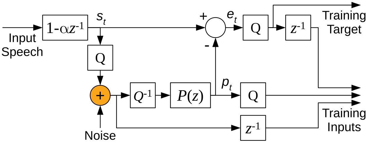
Figure 2: Noise injection during the training procedure, with $Q$ denoting $\mu$-law quantization and $Q^{-1}$ denoting conversion from $\mu$-law to linear. The prediction filter filter $P\left(z\right)=\sum_{k=1}^{M}a_{k}z^{-k}$ is applied to the noisy, quantized input. The excitation is computed as the difference between the clean, unquantized input and the prediction. Note that the noise is added in the $\mu$-law domain.

图 2：训练过程中的噪声注入。$Q$ 表示 $\mu$-law 量化，$Q^{-1}$ 表示从 $\mu$-law 转线性。预测滤波器 $P\left(z\right)=\sum_{k=1}^{M}a_{k}z^{-k}$ 作用于带噪、已量化的输入。激励取干净未量化输入与预测之差。注意噪声加在 $\mu$-law 域。

To make the noise proportional to the signal amplitude, we inject it directly in the $\mu$-law domain. We vary its distribution across the training data from no noise to a uniform distribution in the $\left[-3,3\right]$ range.

为使噪声与信号幅度成比例，我们直接在 $\mu$-law 域注入。噪声分布在训练数据上从无噪变到 $[-3,3]$ 上的均匀分布。

4 Evaluation

4 评估

The source code for this work is available under an open-source license at https://github.com/mozilla/LPCNet/. The evaluation in this section is based on commit 0ddcda0.

本工作的源代码以开源许可发布于 https://github.com/mozilla/LPCNet/。本节评估基于提交 0ddcda0。

4.1 Complexity

4.1 复杂度

The complexity of the proposed LPCNet model mostly comes from the two GRUs as well as the dual fully-connected layer. It corresponds to two operations (one add, one multiply) per weight, for each sample produced and is given by

所提 LPCNet 的复杂度主要来自两个 GRU 以及双重全连接层。对应每个权重对每个产出样本做两次运算（一次加、一次乘），公式为

$$C=\left(3dN_{A}^{2}+3N_{B}\left(N_{A}+N_{B}\right)+2N_{B}Q\right)\cdot 2F_{s}\ , \tag{8}$$

where $N_{A}$ and $N_{B}$ are the sizes of the two GRUs, $d$ is the density of the sparse GRU, $Q$ is the number of $\mu$-law levels and $F_{s}$ is the sampling rate. Using $N_{A}=384$, $N_{B}=16$ and $Q=256$ for wideband speech ($F_{s}=16000$), and considering around 0.5 GFLOPS complexity for the neglected terms (biases, conditioning network, activation functions, …), we obtain a total complexity around 2.8 GFLOPS. Real-time synthesis can be achieved on a single core of an Apple A8 (iPhone 6) or with 20% of a 2.4 GHz Intel Broadwell core.

其中 $N_{A}$、$N_{B}$ 为两个 GRU 的规模，$d$ 为稀疏 GRU 的密度，$Q$ 为 $\mu$-law 电平数，$F_{s}$ 为采样率。对宽带语音取 $N_{A}=384$、$N_{B}=16$、$Q=256$（$F_{s}=16000$），并计入约 0.5 GFLOPS 的忽略项（偏置、条件网络、激活函数等），总复杂度约 2.8 GFLOPS。在 Apple A8（iPhone 6）单核能实时合成，或占用 2.4 GHz Intel Broadwell 单核约 20%。

As a comparison, the speaker-dependent FFTNet model – which claims a lower complexity than the original WaveNet [5] algorithm – has a complexity around 16 GFLOPS [6]. The complexity of the original WaveRNN – evaluated as a speaker-dependent model – is not explicitly stated, but our interpretation of the data provided in the WaveRNN [7] paper suggests a complexity around 10 GFLOPS for the sparse, mobile version. The complexity of SampleRNN is not explicitly stated either, but from the paper, we estimate around 50 GFLOPS (mostly due to the 1024-unit MLP layers).

对比而言，说话人相关的 FFTNet——声称比原始 WaveNet [5] 更低复杂度——约 16 GFLOPS [6]。原始 WaveRNN（按说话人相关模型评估）未明确给出复杂度，但按 [7] 数据我们解读稀疏移动版约 10 GFLOPS。SampleRNN 同样未明示，据论文估计约 50 GFLOPS（主要因 1024 单元 MLP 层）。

4.2 Experimental Setup

4.2 实验设置

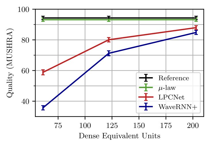
Figure 3: Subjective quality (MUSHRA) results as a function of the dense equivalent number of units in $\mathrm{GRU_{A}}$.

图 3：主观质量（MUSHRA）相对 $\mathrm{GRU_{A}}$ 稠密等价单元数的结果。

Although the proposed system can be either speaker-dependent or speaker-independent, we evaluate it in the more challenging speaker-independent context. To isolate the quality of the vocoder itself, we compute the features directly from recorded speech samples. The cepstrum uses the same band layout as [20] and the pitch estimator is based on an open-loop cross-correlation search.

所提系统既可说话人相关也可说话人无关；我们在更具挑战的说话人无关设定下评估。为单独考察声码器质量，特征直接从录音算出。倒谱带布局与 [20] 相同，基音估计基于开环互相关搜索。

The training data consists of only 4 hours of speech from the NTT Multi-Lingual Speech Database for Telephonometry (21 languages), from which we excluded all samples from the speakers used in testing. Each network was trained for 120 epochs (230k updates), with a batch size size of 64, each sequence consisting of 15 10-ms frames. Training was performed on an Nvidia GPU with Keras[^1]/Tensorflow[^2] using the CuDNN GRU implementation and the AMSGrad [21] optimization method (Adam variant) with a step size $\alpha=\frac{\alpha_{0}}{1+\delta\cdot b}$ where $\alpha_{0}=0.001$, $\delta=5\times 10^{-5},$ and $b$ is the batch number.

训练数据仅用 NTT 多语电话语音库（21 种语言）中约 4 小时语音，并排除全部测试说话人的样本。每个网络训练 120 个 epoch（约 23 万次更新），批大小 64，每条序列含 15 个 10 ms 帧。在 Nvidia GPU 上用 Keras[^1]/Tensorflow[^2] 训练，采用 CuDNN GRU 与 AMSGrad [21]（Adam 变体），步长 $\alpha=\frac{\alpha_{0}}{1+\delta\cdot b}$，其中 $\alpha_{0}=0.001$，$\delta=5\times 10^{-5}$，$b$ 为批序号。

We compare LPCNet to an improved version of WaveRNN (denoted WaveRNN+) that includes all of the improvements in Section 3 except for the LPC part, i.e. WaveRNN+ predicts sample $s_{t}$ only from $s_{t-1}$ and the conditioning parameters. Each model is evaluated with a main GRU of size $N_{A}$ equal to 192, 384, and 640 units, and with a non-zero density $d=0.1$. These have the same number of non-zero weights as equivalent dense GRUs of size 61, 122, and 203, respectively (those GRU sizes match the “equivalent” sizes in [7]). In all cases, the size of the second GRU is $N_{B}=16$. For each test sample, we compute the input features from the original audio (ground truth), and then synthesize new audio with each of the models under test. We also evaluate the effect of the $\mu$-law quantization with pre-emphasis, as an upper-bound for the achievable quality.

我们把 LPCNet 与改进版 WaveRNN（记 WaveRNN+）对比：后者包含第 3 节除 LPC 外的全部改进，即仅由 $s_{t-1}$ 与条件参数预测样本 $s_{t}$。各模型主 GRU 规模 $N_{A}$ 取 192、384、640，非零密度 $d=0.1$，非零权重数分别等价于规模 61、122、203 的稠密 GRU（与 [7] 中「等价」规模一致）。第二 GRU 一律 $N_{B}=16$。每个测试样本从原始音频（真值）算输入特征，再由各待测模型合成新音频。我们也评估带预加重的 $\mu$-law 量化效果，作为可达质量的上界。

4.3 Quality Evaluation

4.3 质量评估

As reported in [4], objective quality metrics such as PESQ and POLQA cannot adequately evaluate non-waveform, neural vocoders. We conducted a subjective listening test with a MUSHRA-derived methodology [22], where 8 utterances (2 male and 2 female speakers) were each evaluated by 100 participants. The results in Fig. 3 show that the quality of LPCNet significantly exceeds that of WaveRNN+ at equal complexity. Alternatively, it shows that the same quality is possible at a significantly reduced complexity. The results also validate our assumption that pre-emphasis makes the effect of $\mu$-law quantization noise negligible compared to the synthesis artifacts. Being able to compute only a single 256-value distribution also reduces complexity compared to the original 16-bit WaveRNN.

如 [4] 所述，PESQ、POLQA 等客观指标不足以评估非波形神经声码器。我们采用源自 MUSHRA 的主观听测方法 [22]：8 条语句（2 男 2 女说话人）各由 100 名受试者评分。图 3 显示，同等复杂度下 LPCNet 质量显著高于 WaveRNN+；或者说，达到相同质量时复杂度可明显降低。结果也验证了预加重使 $\mu$-law 量化噪声相对合成伪影可忽略。只需计算单个 256 值分布，也比原始 16 比特 WaveRNN 更省算力。

The main audible artifact in the generated samples – from both WaveRNN+ and LPCNet – is some roughness due to noise between pitch harmonics. One possible remedy – which we did not yet investigate – consists of using post-denoising techniques, as suggested in [6]. A subset of the samples used in the listening test is available at https://people.xiph.org/˜jm/demo/lpcnet/.

生成样本（WaveRNN+ 与 LPCNet 皆然）中主要可闻伪影是基音谐波之间噪声带来的粗糙感。一种可能补救——我们尚未研究——是采用 [6] 建议的后置去噪。听测所用样本子集见 https://people.xiph.org/~jm/demo/lpcnet/。

5 Conclusion

5 结论

This work demonstrates that the efficiency of speaker-independent speech synthesis can be improved by combining newer neural synthesis techniques with the much older technique of linear prediction. In addition to the main contribution of combining linear prediction with WaveRNN, we make other contributions, such as the embedding of the signal values, the improved sampling, as well as the pre-emphasis prior to $\mu$-law quantization. We believe that the proposed model is equally applicable to text-to-speech and to low-bitrate speech coding.

本工作表明：把较新的神经合成技术与更早的线性预测相结合，可提升说话人无关语音合成的效率。除将线性预测与 WaveRNN 结合这一主贡献外，我们还提出信号值嵌入、改进采样，以及 $\mu$-law 量化前的预加重。我们认为该模型同样适用于文本到语音与低比特率语音编码。

Future work on LPCNet includes investigating whether long-term (pitch) prediction can be incorporated as a way to further reduce the complexity.

LPCNet 的后续工作包括研究能否引入长时（基音）预测以进一步降低复杂度。

References

参考文献

[1] J. Shen, R. Pang, R. J. Weiss, M. Schuster, N. Jaitly, Z. Yang, Z. Chen, Y. Zhang, Y. Wang, R. Skerrv-Ryan, et al., “Natural TTS synthesis by conditioning WaveNet on mel spectrogram predictions,” in Proc. International Conference on Acoustics, Speech, and Signal Processing (ICASSP) , 2018, pp. 4779–4783.

[2] S. Arik, G. Diamos, A. Gibiansky, J. Miller, K. Peng, W. Ping, J. Raiman, and Y. Zhou, “Deep voice 2: Multi-speaker neural text-to-speech,” arXiv:1705.08947 , 2017.

[3] J. Sotelo, S. Mehri, K. Kumar, J. F. Santos, K. Kastner, A. Courville, and Y. Bengio, “Char2wav: End-to-end speech synthesis,” in Proc. ICLR Workshop , 2017.

[4] W. B. Kleijn, F. SC Lim, A. Luebs, J. Skoglund, F. Stimberg, Q. Wang, and T. C. Walters, “WaveNet based low rate speech coding,” in Proc. International Conference on Acoustics, Speech, and Signal Processing (ICASSP) , 2018, pp. 676–680.

[5] A. van den Oord, S. Dieleman, H. Zen, K. Simonyan, O. Vinyals, A. Graves, N. Kalchbrenner, A. Senior, and K. Kavukcuoglu, “WaveNet: A generative model for raw audio,” arXiv:1609.03499 , 2016.

[6] Z. Jin, A. Finkelstein, G. J. Mysore, and J. Lu, “FFTNet: A real-time speaker-dependent neural vocoder,” in Proc. International Conference on Acoustics, Speech, and Signal Processing (ICASSP) , 2018, pp. 2251–2255.

[7] N. Kalchbrenner, E. Elsen, K. Simonyan, S. Noury, N. Casagrande, E. Lockhart, F. Stimberg, A. van den Oord, S. Dieleman, and K. Kavukcuoglu, “Efficient neural audio synthesis,” arXiv:1802.08435 , 2018.

[8] B. S. Atal and S. L. Hanauer, “Speech analysis and synthesis by linear prediction of the speech wave,” The journal of the acoustical society of America , vol. 50, no. 2B, pp. 637–655, 1971.

[9] J. Markel and A. Gray, “A linear prediction vocoder simulation based upon the autocorrelation method,” IEEE Transactions on Acoustics, Speech, and Signal Processing , vol. 22, no. 2, pp. 124–134, 1974.

[10] D. Griffin and J. Lim, “A new model-based speech analysis/synthesis system,” in Proc. International Conference on Acoustics, Speech, and Signal Processing (ICASSP) , 1985, vol. 10, pp. 513–516.

[11] A. McCree, K. Truong, E. B. George, T. P. Barnwell, and V. Viswanathan, “A 2.4 kbit/s MELP coder candidate for the new us federal standard,” in Proc. International Conference on Acoustics, Speech, and Signal Processing (ICASSP) , 1996, vol. 1, pp. 200–203.

[12] L. Juvela, V. Tsiaras, B. Bollepalli, M. Airaksinen, J. Yamagishi, and P. Alku, “Speaker-independent raw waveform model for glottal excitation,” in Proc. Interspeech , 2018, pp. 2012–2016.

[13] K. Cho, B. Van Merriënboer, D. Bahdanau, and Y. Bengio, “On the properties of neural machine translation: Encoder-decoder approaches,” in Proc. Eighth Workshop on Syntax, Semantics and Structure in Statistical Translation (SSST-8) , 2014.

[14] B.C.J. Moore, An introduction to the psychology of hearing , Brill, fifth edition, 2012.

[15] ITU-T, Recommendation G.711: Pulse Code Modulation (PCM) of voice frequencies , International Telecommunications Union, 1988.

[16] S. Mehri, K. Kumar, I. Gulrajani, R. Kumar, S. Jain, J. Sotelo, A. Courville, and Y. Bengio, “SampleRNN: An unconditional end-to-end neural audio generation model,” arXiv:1612.07837 , 2016.

[17] J. Makhoul, “Linear prediction: A tutorial review,” Proc. IEEE , vol. 63, no. 4, pp. 561–580, 1975.

[18] B. S. Atal and J. Remde, “A new model of LPC excitation for producing natural-sounding speech at low bit rates,” in Proc. International Conference on Acoustics, Speech, and Signal Processing (ICASSP) , 1982, vol. 7, pp. 614–617.

[19] M. Schroeder and B.S. Atal, “Code-excited linear prediction (CELP): High-quality speech at very low bit rates,” in Proc. International Conference on Acoustics, Speech, and Signal Processing (ICASSP) , 1985, vol. 10, pp. 937–940.

[20] J.-M. Valin, “A hybrid DSP/deep learning approach to real-time full-band speech enhancement,” in Proc. Multimedia Signal Processing Workshop (MMSP) , 2018.

[21] S. J. Reddi, S. Kale, and S. Kumar, “On the convergence of adam and beyond,” in Proc. ICLR , 2018.

[22] ITU-R, Recommendation BS.1534-1: Method for the subjective assessment of intermediate quality level of coding systems , International Telecommunications Union, 2001.