The Lottery Ticket Hypothesis: Finding Sparse, Trainable Neural Networks

彩票假设：寻找稀疏且可训练的神经网络

Jonathan Frankle Affiliation:  MIT CSAIL Email:  jfrankle@csail.mit.edu    Michael Carbin Affiliation:  MIT CSAIL Email:  mcarbin@csail.mit.edu

Abstract

摘要

Neural network pruning techniques can reduce the parameter counts of trained networks by over 90%, decreasing storage requirements and improving computational performance of inference without compromising accuracy. However, contemporary experience is that the sparse architectures produced by pruning are difficult to train from the start, which would similarly improve training performance.

神经网络剪枝技术可以把已训练网络的参数量减少 90% 以上，从而降低存储需求、提高推理的计算性能，同时不牺牲精度。不过当代经验是：剪枝得到的稀疏结构很难从一开始就训练好，而若能做到，训练效率同样会提高。

We find that a standard pruning technique naturally uncovers subnetworks whose initializations made them capable of training effectively. Based on these results, we articulate the lottery ticket hypothesis: dense, randomly-initialized, feed-forward networks contain subnetworks (winning tickets) that—when trained in isolation—reach test accuracy comparable to the original network in a similar number of iterations. The winning tickets we find have won the initialization lottery: their connections have initial weights that make training particularly effective.

我们发现，一种标准剪枝技术会自然地揭示出一些子网络，它们的初始化使这些子网络能够有效地训练。基于这些结果，我们提出彩票假设：稠密、随机初始化的前馈网络中包含这样的子网络（中奖彩票）——当它们被单独训练时，能在相近的迭代次数内达到与原网络相当的测试精度。我们找到的中奖彩票赢在了初始化：它们的连接带有使训练特别有效的初始权重。

We present an algorithm to identify winning tickets and a series of experiments that support the lottery ticket hypothesis and the importance of these fortuitous initializations. We consistently find winning tickets that are less than 10-20% of the size of several fully-connected and convolutional feed-forward architectures for MNIST and CIFAR10. Above this size, the winning tickets that we find learn faster than the original network and reach higher test accuracy.

我们给出识别中奖彩票的算法，以及一系列支持彩票假设、并说明这些幸运初始化很重要的实验。在若干用于 MNIST 和 CIFAR10 的全连接与卷积前馈结构上，我们稳定地找到大小不到原网络 10–20% 的中奖彩票。大于这一规模时，我们找到的中奖彩票比原网络学得更快，测试精度也更高。

1 Introduction

1 引言

Techniques for eliminating unnecessary weights from neural networks (pruning) (LeCun et al., 1990; Hassibi & Stork, 1993; Han et al., 2015; Li et al., 2016) can reduce parameter-counts by more than 90% without harming accuracy. Doing so decreases the size (Han et al., 2015; Hinton et al., 2015) or energy consumption (Yang et al., 2017; Molchanov et al., 2016; Luo et al., 2017) of the trained networks, making inference more efficient. However, if a network can be reduced in size, why do we not train this smaller architecture instead in the interest of making training more efficient as well? Contemporary experience is that the architectures uncovered by pruning are harder to train from the start, reaching lower accuracy than the original networks.[^1]

从神经网络中剔除不必要权重的技术（剪枝）（LeCun et al., 1990; Hassibi & Stork, 1993; Han et al., 2015; Li et al., 2016）可以把参数量减少 90% 以上而不损害精度。这样做会减小已训练网络的体积（Han et al., 2015; Hinton et al., 2015）或能耗（Yang et al., 2017; Molchanov et al., 2016; Luo et al., 2017），使推理更高效。可是，如果网络可以被缩小，我们为什么不直接训练这个更小的结构，好让训练也更高效？当代经验是：剪枝揭示出的结构更难从一开始训练，达到的精度也低于原网络。[^1]

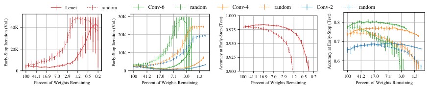
Figure 1: The iteration at which early-stopping would occur (left) and the test accuracy at that iteration (right) of the Lenet architecture for MNIST and the Conv-2, Conv-4, and Conv-6 architectures for CIFAR10 (see Figure 2) when trained starting at various sizes. Dashed lines are randomly sampled sparse networks (average of ten trials). Solid lines are winning tickets (average of five trials).

图 1：在多种起始规模下训练时，用于 MNIST 的 Lenet 以及用于 CIFAR10 的 Conv-2、Conv-4 和 Conv-6（见图 2）会触发早停的迭代（左）以及该迭代上的测试精度（右）。虚线是随机采样的稀疏网络（十次试验的平均）。实线是中奖彩票（五次试验的平均）。

Consider an example. In Figure 1, we randomly sample and train subnetworks from a fully-connected network for MNIST and convolutional networks for CIFAR10. Random sampling models the effect of the unstructured pruning used by LeCun et al. (1990) and Han et al. (2015). Across various levels of sparsity, dashed lines trace the iteration of minimum validation loss[^2] and the test accuracy at that iteration. The sparser the network, the slower the learning and the lower the eventual test accuracy.

看一个例子。在图 1 中，我们从用于 MNIST 的全连接网络和用于 CIFAR10 的卷积网络中随机采样子网络并训练。随机采样建模的是 LeCun 等人（1990）和 Han 等人（2015）所用的非结构化剪枝的效果。在不同稀疏程度上，虚线标出验证损失最低的迭代[^2]以及该迭代上的测试精度。网络越稀疏，学习就越慢，最终测试精度也越低。

In this paper, we show that there consistently exist smaller subnetworks that train from the start and learn at least as fast as their larger counterparts while reaching similar test accuracy. Solid lines in Figure 1 show networks that we find. Based on these results, we state the lottery ticket hypothesis.

本文中我们表明：始终存在更小的子网络，它们从一开始就能训练，学习速度至少不慢于更大的对应网络，并能达到相近的测试精度。图 1 中的实线就是我们找到的这类网络。基于这些结果，我们提出彩票假设。

The Lottery Ticket Hypothesis.

A randomly-initialized, dense neural network contains a subnetwork that is initialized such that—when trained in isolation—it can match the test accuracy of the original network after training for at most the same number of iterations.

彩票假设。

一个随机初始化的稠密神经网络中，包含这样一个被初始化好的子网络：当它被单独训练时，至多只需与原网络相同的迭代次数，就能匹配原网络训练后的测试精度。

More formally, consider a dense feed-forward neural network $f(x;\theta)$ with initial parameters $\theta=\theta_{0}\sim\mathcal{D}_{\theta}$. When optimizing with stochastic gradient descent (SGD) on a training set, $f$ reaches minimum validation loss $l$ at iteration $j$ with test accuracy $a$ . In addition, consider training $f(x;m\odot\theta)$ with a mask $m\in\{0,1\}^{|\theta|}$ on its parameters such that its initialization is $m\odot\theta_{0}$. When optimizing with SGD on the same training set (with $m$ fixed), $f$ reaches minimum validation loss $l^{\prime}$ at iteration $j^{\prime}$ with test accuracy $a^{\prime}$. The lottery ticket hypothesis predicts that $\exists~m$ for which $j^{\prime}\leq j$ (commensurate training time), $a^{\prime}\geq a$ (commensurate accuracy), and $\lVert m\rVert_{0}\ll|\theta|$ (fewer parameters).

更形式化地说，考虑一个稠密前馈神经网络 $f(x;\theta)$，初始参数为 $\theta=\theta_{0}\sim\mathcal{D}_{\theta}$。在训练集上用随机梯度下降（SGD）优化时，$f$ 在迭代 $j$ 达到最低验证损失 $l$，测试精度为 $a$。此外，考虑用参数掩码 $m\in\{0,1\}^{|\theta|}$ 来训练 $f(x;m\odot\theta)$，使其初始化为 $m\odot\theta_{0}$。在同一训练集上用 SGD 优化（$m$ 固定）时，$f$ 在迭代 $j^{\prime}$ 达到最低验证损失 $l^{\prime}$，测试精度为 $a^{\prime}$。彩票假设预言：存在掩码 $m$，使得 $j^{\prime}\leq j$（相当的训练时间）、$a^{\prime}\geq a$（相当的精度），并且 $\lVert m\rVert_{0}\ll|\theta|$（参数更少）。

We find that a standard pruning technique automatically uncovers such trainable subnetworks from fully-connected and convolutional feed-forward networks. We designate these trainable subnetworks, $f(x;m\odot\theta_{0})$, winning tickets, since those that we find have won the initialization lottery with a combination of weights and connections capable of learning. When their parameters are randomly reinitialized ($f(x;m\odot\theta^{\prime}_{0})$ where $\theta^{\prime}_{0}\sim\mathcal{D}_{\theta}$), our winning tickets no longer match the performance of the original network, offering evidence that these smaller networks do not train effectively unless they are appropriately initialized.

我们发现，一种标准剪枝技术会自动从全连接和卷积前馈网络中揭示出这类可训练子网络。我们把这些可训练子网络 $f(x;m\odot\theta_{0})$ 称为中奖彩票，因为我们找到的那些已经赢了初始化彩票：它们拥有一组能够学习的权重与连接组合。当它们的参数被随机重新初始化（$f(x;m\odot\theta^{\prime}_{0})$，其中 $\theta^{\prime}_{0}\sim\mathcal{D}_{\theta}$）时，我们的中奖彩票便不再匹配原网络的表现，这提供了证据：这些更小的网络除非被恰当地初始化，否则无法有效训练。

Identifying winning tickets. We identify a winning ticket by training a network and pruning its smallest-magnitude weights. The remaining, unpruned connections constitute the architecture of the winning ticket. Unique to our work, each unpruned connection’s value is then reset to its initialization from original network before it was trained. This forms our central experiment:

识别中奖彩票。 我们通过训练一个网络并剪去幅度最小的权重来识别中奖彩票。剩下未被剪掉的连接构成中奖彩票的结构。与以往工作不同的是，每个未被剪掉的连接随后会被重置为原网络训练之前的初始化取值。这就构成了我们的核心实验：

1. Randomly initialize a neural network $f(x;\theta_{0})$ (where $\theta_{0}\sim\mathcal{D}_{\theta}$).

1. 随机初始化一个神经网络 $f(x;\theta_{0})$（其中 $\theta_{0}\sim\mathcal{D}_{\theta}$）。

2. Train the network for $j$ iterations, arriving at parameters $\theta_{j}$.

2. 将网络训练 $j$ 次迭代，得到参数 $\theta_{j}$。

3. Prune $p\%$ of the parameters in $\theta_{j}$, creating a mask $m$.

3. 剪掉 $\theta_{j}$ 中 $p\%$ 的参数，得到掩码 $m$。

4. Reset the remaining parameters to their values in $\theta_{0}$, creating the winning ticket $f(x;m\odot\theta_{0})$.

4. 把剩下的参数重置为它们在 $\theta_{0}$ 中的取值，得到中奖彩票 $f(x;m\odot\theta_{0})$。

As described, this pruning approach is one-shot: the network is trained once, $p\%$ of weights are pruned, and the surviving weights are reset. However, in this paper, we focus on iterative pruning, which repeatedly trains, prunes, and resets the network over $n$ rounds; each round prunes $p^{\frac{1}{n}}\%$ of the weights that survive the previous round. Our results show that iterative pruning finds winning tickets that match the accuracy of the original network at smaller sizes than does one-shot pruning.

按上述方式，这种剪枝是一次性的：网络训练一次，剪掉 $p\%$ 的权重，再把存活的权重重置。不过本文关注的是迭代剪枝：在 $n$ 轮中反复训练、剪枝并重置网络；每一轮剪掉上一轮存活权重的 $p^{\frac{1}{n}}\%$。我们的结果表明，迭代剪枝能在比一次性剪枝更小的规模上，找到匹配原网络精度的中奖彩票。

Results. We identify winning tickets in a fully-connected architecture for MNIST and convolutional architectures for CIFAR10 across several optimization strategies (SGD, momentum, and Adam) with techniques like dropout, weight decay, batchnorm, and residual connections. We use an unstructured pruning technique, so these winning tickets are sparse. In deeper networks, our pruning-based strategy for finding winning tickets is sensitive to the learning rate: it requires warmup to find winning tickets at higher learning rates. The winning tickets we find are 10-20% (or less) of the size of the original network (smaller size). Down to that size, they meet or exceed the original network’s test accuracy (commensurate accuracy) in at most the same number of iterations (commensurate training time). When randomly reinitialized, winning tickets perform far worse, meaning structure alone cannot explain a winning ticket’s success.

结果。 我们在用于 MNIST 的全连接结构和用于 CIFAR10 的卷积结构中识别出中奖彩票，覆盖若干优化策略（SGD、动量和 Adam）以及 dropout、权重衰减、批归一化和残差连接等技术。我们使用非结构化剪枝，因此这些中奖彩票是稀疏的。在更深的网络中，我们这种基于剪枝寻找中奖彩票的策略对学习率敏感：在较高学习率下需要预热才能找到中奖彩票。我们找到的中奖彩票是原网络大小的 10–20%（或更小）（更小的规模）。在降到这一规模之前，它们能在至多相同的迭代次数内（相当的训练时间）达到或超过原网络的测试精度（相当的精度）。随机重新初始化后，中奖彩票的表现差得多，说明单靠结构无法解释一张中奖彩票为何成功。

The Lottery Ticket Conjecture. Returning to our motivating question, we extend our hypothesis into an untested conjecture that SGD seeks out and trains a subset of well-initialized weights. Dense, randomly-initialized networks are easier to train than the sparse networks that result from pruning because there are more possible subnetworks from which training might recover a winning ticket.

彩票猜想。 回到最初那个问题，我们把假设延伸成一个尚未检验的猜想：SGD 会寻找并训练一小部分集合初始化良好的权重。稠密、随机初始化的网络比剪枝得到的稀疏网络更容易训练，是因为可能从中恢复出中奖彩票的子网络组合更多。

Contributions.

贡献。

• • We demonstrate that pruning uncovers trainable subnetworks that reach test accuracy comparable to the original networks from which they derived in a comparable number of iterations.

• • 我们表明，剪枝能够揭示可训练的子网络，它们在相当的迭代次数内达到与其所源自的原网络相当的测试精度。

• • We show that pruning finds winning tickets that learn faster than the original network while reaching higher test accuracy and generalizing better.

• • 我们表明，剪枝找到的中奖彩票比原网络学得更快，测试精度更高，泛化也更好。

• • We propose the lottery ticket hypothesis as a new perspective on the composition of neural networks to explain these findings.

• • 我们提出彩票假设，作为一种理解神经网络构成的新视角，来解释这些发现。

Implications. In this paper, we empirically study the lottery ticket hypothesis. Now that we have demonstrated the existence of winning tickets, we hope to exploit this knowledge to:

含义。 本文从经验上研究彩票假设。既然我们已经表明中奖彩票存在，便希望利用这一认识来：

Improve training performance. Since winning tickets can be trained from the start in isolation, a hope is that we can design training schemes that search for winning tickets and prune as early as possible.

提高训练性能。 由于中奖彩票可以从一开始就被单独训练，一个希望是我们可以设计训练方案，去搜索中奖彩票并尽早剪枝。

Design better networks. Winning tickets reveal combinations of sparse architectures and initializations that are particularly adept at learning. We can take inspiration from winning tickets to design new architectures and initialization schemes with the same properties that are conducive to learning. We may even be able to transfer winning tickets discovered for one task to many others.

设计更好的网络。 中奖彩票揭示了特别擅长学习的稀疏结构与初始化组合。我们可以从中奖彩票获得启发，设计具有同样有利于学习之性质的新结构和初始化方案。我们甚至可能把为一项任务发现的中奖彩票迁移到许多其他任务上。

Improve our theoretical understanding of neural networks. We can study why randomly-initialized feed-forward networks seem to contain winning tickets and potential implications for theoretical study of optimization (Du et al., 2019) and generalization (Zhou et al., 2018; Arora et al., 2018).

增进我们对神经网络的理论理解。 我们可以研究随机初始化的前馈网络为何似乎包含中奖彩票，以及这对优化（Du et al., 2019）和泛化（Zhou et al., 2018; Arora et al., 2018）的理论研究可能意味着什么。

2 Winning Tickets in Fully-Connected Networks

2 全连接网络中的中奖彩票

Network	Lenet	Conv-2	Conv-4	Conv-6	Resnet-18	VGG-19
Convolutions		64, 64, pool	64, 64, pool 128, 128, pool	64, 64, pool 128, 128, pool 256, 256, pool	16, 3x[16, 16] 3x[32, 32] 3x[64, 64]	2x64 pool 2x128 pool, 4x256, pool 4x512, pool, 4x512
FC Layers	300, 100, 10	256, 256, 10	256, 256, 10	256, 256, 10	avg-pool, 10	avg-pool, 10
All/Conv Weights	266K	4.3M / 38K	2.4M / 260K	1.7M / 1.1M	274K / 270K	20.0M
Iterations/Batch	50K / 60	20K / 60	25K / 60	30K / 60	30K / 128	112K / 64
Optimizer	Adam 1.2e-3	Adam 2e-4	Adam 3e-4	Adam 3e-4	$\leftarrow$ SGD 0.1-0.01-0.001 Momentum 0.9 $\rightarrow$
Pruning Rate	fc20%	conv10% fc20%	conv10% fc20%	conv15% fc20%	conv20% fc0%	conv20% fc0%

Figure 2: Architectures tested in this paper. Convolutions are 3x3. Lenet is from LeCun et al. (1998). Conv-2/4/6 are variants of VGG (Simonyan & Zisserman, 2014). Resnet-18 is from He et al. (2016). VGG-19 for CIFAR10 is adapted from Liu et al. (2019). Initializations are Gaussian Glorot (Glorot & Bengio, 2010). Brackets denote residual connections around layers.

网络	Lenet	Conv-2	Conv-4	Conv-6	Resnet-18	VGG-19
卷积		64, 64, pool	64, 64, pool 128, 128, pool	64, 64, pool 128, 128, pool 256, 256, pool	16, 3x[16, 16] 3x[32, 32] 3x[64, 64]	2x64 pool 2x128 pool, 4x256, pool 4x512, pool, 4x512
全连接层	300, 100, 10	256, 256, 10	256, 256, 10	256, 256, 10	avg-pool, 10	avg-pool, 10
全部/卷积权重	266K	4.3M / 38K	2.4M / 260K	1.7M / 1.1M	274K / 270K	20.0M
迭代/批次	50K / 60	20K / 60	25K / 60	30K / 60	30K / 128	112K / 64
优化器	Adam 1.2e-3	Adam 2e-4	Adam 3e-4	Adam 3e-4	$\leftarrow$ SGD 0.1-0.01-0.001 Momentum 0.9 $\rightarrow$
剪枝率	fc20%	conv10% fc20%	conv10% fc20%	conv15% fc20%	conv20% fc0%	conv20% fc0%

图 2：本文测试的网络结构。卷积核为 3x3。Lenet 来自 LeCun 等人（1998）。Conv-2/4/6 是 VGG 的变体（Simonyan & Zisserman, 2014）。Resnet-18 来自 He 等人（2016）。用于 CIFAR10 的 VGG-19 改编自 Liu 等人（2019）。初始化为高斯 Glorot（Glorot & Bengio, 2010）。方括号表示层周围的残差连接。

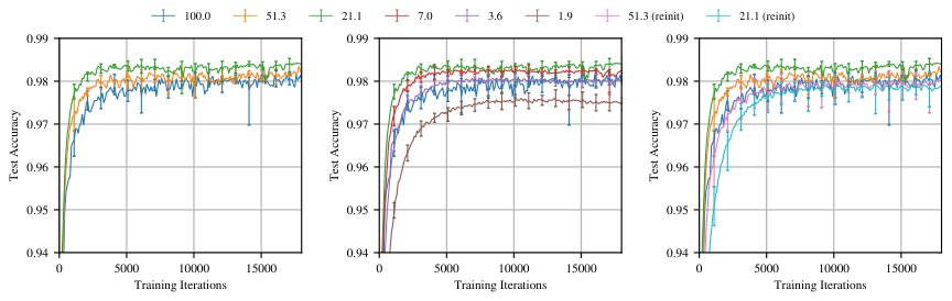
Figure 3: Test accuracy on Lenet (iterative pruning) as training proceeds. Each curve is the average of five trials. Labels are $P_{m}$—the fraction of weights remaining in the network after pruning. Error bars are the minimum and maximum of any trial.

图 3：Lenet 上（迭代剪枝）训练过程中的测试精度。每条曲线是五次试验的平均。标签为 $P_{m}$——剪枝后网络中剩余权重的比例。误差条是各次试验的最小与最大值。

In this Section, we assess the lottery ticket hypothesis as applied to fully-connected networks trained on MNIST. We use the Lenet-300-100 architecture (LeCun et al., 1998) as described in Figure 2. We follow the outline from Section 1: after randomly initializing and training a network, we prune the network and reset the remaining connections to their original initializations. We use a simple layer-wise pruning heuristic: remove a percentage of the weights with the lowest magnitudes within each layer (as in Han et al. (2015)). Connections to outputs are pruned at half of the rate of the rest of the network. We explore other hyperparameters in Appendix G, including learning rates, optimization strategies (SGD, momentum), initialization schemes, and network sizes.

本节评估彩票假设在 MNIST 上训练的全连接网络中的表现。我们使用图 2 中描述的 Lenet-300-100 结构（LeCun et al., 1998）。我们遵循第 1 节的提纲：在随机初始化并训练一个网络之后，对其剪枝，并把剩下的连接重置为原来的初始化。我们使用一种简单的逐层剪枝启发式：在每一层内去掉幅度最低的一部分权重（与 Han 等人（2015）类似）。连到输出的连接以网络其余部分一半的比率剪枝。我们在附录 G 中探讨了其他超参数，包括学习率、优化策略（SGD、动量）、初始化方案和网络规模。

Notation. $P_{m}=\frac{\lVert m\rVert_{0}}{|\theta|}$ is the sparsity of mask $m$, e.g., $P_{m}=25\%$ when 75% of weights are pruned.

记号。 $P_{m}=\frac{\lVert m\rVert_{0}}{|\theta|}$ 是掩码 $m$ 的稀疏度，例如当 75% 的权重被剪掉时，$P_{m}=25\%$。

Iterative pruning. The winning tickets we find learn faster than the original network. Figure 3 plots the average test accuracy when training winning tickets iteratively pruned to various extents. Error bars are the minimum and maximum of five runs. For the first pruning rounds, networks learn faster and reach higher test accuracy the more they are pruned (left graph in Figure 3). A winning ticket comprising 51.3% of the weights from the original network (i.e., $P_{m}=51.3\%$) reaches higher test accuracy faster than the original network but slower than when $P_{m}=21.1\%$. When $P_{m}<21.1\%$, learning slows (middle graph). When $P_{m}=3.6\%$, a winning ticket regresses to the performance of the original network. A similar pattern repeats throughout this paper.

迭代剪枝。 我们找到的中奖彩票比原网络学得更快。图 3 画出了迭代剪枝到不同程度时，训练中奖彩票的平均测试精度。误差条是五次运行的最小与最大值。在最初几轮剪枝中，网络被剪得越多，就学得越快、测试精度也越高（图 3 左图）。一张包含原网络 51.3% 权重的中奖彩票（即 $P_{m}=51.3\%$）比原网络更快达到更高测试精度，但比 $P_{m}=21.1\%$ 时更慢。当 $P_{m}<21.1\%$ 时，学习变慢（中图）。当 $P_{m}=3.6\%$ 时，中奖彩票回退到原网络的表现。类似的模式在本文中反复出现。

Figure 4a summarizes this behavior for all pruning levels when iteratively pruning by 20% per iteration (blue). On the left is the iteration at which each network reaches minimum validation loss (i.e., when the early-stopping criterion would halt training) in relation to the percent of weights remaining after pruning; in the middle is test accuracy at that iteration. We use the iteration at which the early-stopping criterion is met as a proxy for how quickly the network learns.

图 4a 在每一轮迭代剪枝 20% 时（蓝色），概括了所有剪枝水平上的这一行为。左边是每个网络达到最低验证损失的迭代（也就是早停准则会停止训练的时刻）与剪枝后剩余权重百分比的关系；中间是该迭代上的测试精度。我们把达到早停准则的迭代当作网络学习有多快的代理指标。

The winning tickets learn faster as $P_{m}$ decreases from 100% to 21%, at which point early-stopping occurs $38\%$ earlier than for the original network. Further pruning causes learning to slow, returning to the early-stopping performance of the original network when $P_{m}=3.6\%$. Test accuracy increases with pruning, improving by more than 0.3 percentage points when $P_{m}=13.5\%$; after this point, accuracy decreases, returning to the level of the original network when $P_{m}=3.6\%$.

随着 $P_{m}$ 从 100% 降到 21%，中奖彩票学得更快，此时早停比原网络早 $38\%$。继续剪枝会使学习变慢，当 $P_{m}=3.6\%$ 时回到原网络的早停表现。测试精度随剪枝上升，在 $P_{m}=13.5\%$ 时提高超过 0.3 个百分点；过了这一点精度下降，当 $P_{m}=3.6\%$ 时回到原网络的水平。

At early stopping, training accuracy (Figure 4a, right) increases with pruning in a similar pattern to test accuracy, seemingly implying that winning tickets optimize more effectively but do not generalize better. However, at iteration 50,000 (Figure 4b), iteratively-pruned winning tickets still see a test accuracy improvement of up to 0.35 percentage points in spite of the fact that training accuracy reaches 100% for nearly all networks (Appendix D, Figure 12). This means that the gap between training accuracy and test accuracy is smaller for winning tickets, pointing to improved generalization.

在早停时，训练精度（图 4a，右）随剪枝上升，模式与测试精度相似，这似乎意味着中奖彩票优化得更有效，但泛化并不更好。然而在第 50,000 次迭代（图 4b），迭代剪枝得到的中奖彩票仍有最高 0.35 个百分点的测试精度提升，尽管几乎所有网络的训练精度都达到了 100%（附录 D，图 12）。这意味着中奖彩票的训练精度与测试精度之间的差距更小，指向更好的泛化。

Random reinitialization. To measure the importance of a winning ticket’s initialization, we retain the structure of a winning ticket (i.e., the mask $m$) but randomly sample a new initialization $\theta^{\prime}_{0}\sim\mathcal{D}_{\theta}$. We randomly reinitialize each winning ticket three times, making 15 total per point in Figure 4. We find that initialization is crucial for the efficacy of a winning ticket. The right graph in Figure 3 shows this experiment for iterative pruning. In addition to the original network and winning tickets at $P_{m}=51\%$ and $21\%$ are the random reinitialization experiments. Where the winning tickets learn faster as they are pruned, they learn progressively slower when randomly reinitialized.

随机重新初始化。 为了衡量中奖彩票初始化的重要性，我们保留中奖彩票的结构（即掩码 $m$），但重新随机采样一个初始化 $\theta^{\prime}_{0}\sim\mathcal{D}_{\theta}$。我们对每张中奖彩票随机重新初始化三次，使图 4 中每个点共有 15 次试验。我们发现，初始化对中奖彩票是否有效至关重要。图 3 右图展示了迭代剪枝下的这一实验。除了原网络以及 $P_{m}=51\%$ 和 $21\%$ 的中奖彩票之外，还有随机重新初始化实验。中奖彩票随着被剪枝而学得更快，随机重新初始化后则越学越慢。

The broader results of this experiment are orange line in Figure 4a. Unlike winning tickets, the reinitialized networks learn increasingly slower than the original network and lose test accuracy after little pruning. The average reinitialized iterative winning ticket’s test accuracy drops off from the original accuracy when $P_{m}=21.1\%$, compared to 2.9% for the winning ticket. When $P_{m}=21\%$, the winning ticket reaches minimum validation loss 2.51x faster than when reinitialized and is half a percentage point more accurate. All networks reach 100% training accuracy for $P_{m}\geq 5\%$; Figure 4b therefore shows that the winning tickets generalize substantially better than when randomly reinitialized. This experiment supports the lottery ticket hypothesis’ emphasis on initialization: the original initialization withstands and benefits from pruning, while the random reinitialization’s performance immediately suffers and diminishes steadily.

这一实验更全面的结果是图 4a 中的橙色线。与中奖彩票不同，重新初始化的网络比原网络学得越来越慢，并且只需很少剪枝就会损失测试精度。平均而言，重新初始化的迭代中奖彩票在 $P_{m}=21.1\%$ 时测试精度就从原精度掉下去，而中奖彩票要到 2.9%。当 $P_{m}=21\%$ 时，中奖彩票达到最低验证损失的速度是重新初始化时的 2.51 倍，精度也高出半个百分点。所有网络在 $P_{m}\geq 5\%$ 时都达到 100% 训练精度；因此图 4b 表明，中奖彩票的泛化明显好于随机重新初始化。这一实验支持彩票假设对初始化的强调：原来的初始化经得起剪枝并从中受益，而随机重新初始化的表现立刻受损，并稳步下降。

One-shot pruning. Although iterative pruning extracts smaller winning tickets, repeated training means they are costly to find. One-shot pruning makes it possible to identify winning tickets without this repeated training. Figure 4c shows the results of one-shot pruning (green) and randomly reinitializing (red); one-shot pruning does indeed find winning tickets. When $67.5\%\geq P_{m}\geq 17.6\%$, the average winning tickets reach minimum validation accuracy earlier than the original network. When $95.0\%\geq P_{m}\geq 5.17\%$, test accuracy is higher than the original network. However, iteratively-pruned winning tickets learn faster and reach higher test accuracy at smaller network sizes. The green and red lines in Figure 4c are reproduced on the logarithmic axes of Figure 4a, making this performance gap clear. Since our goal is to identify the smallest possible winning tickets, we focus on iterative pruning throughout the rest of the paper.

一次性剪枝。 尽管迭代剪枝能抽出更小的中奖彩票，反复训练意味着寻找它们的代价很高。一次性剪枝使得不必反复训练就能识别中奖彩票。图 4c 展示了一次性剪枝（绿色）和随机重新初始化（红色）的结果；一次性剪枝确实能找到中奖彩票。当 $67.5\%\geq P_{m}\geq 17.6\%$ 时，平均中奖彩票比原网络更早达到最低验证精度。当 $95.0\%\geq P_{m}\geq 5.17\%$ 时，测试精度高于原网络。不过，迭代剪枝得到的中奖彩票在更小的网络规模上学得更快、测试精度也更高。图 4c 中的绿线和红线被复现到图 4a 的对数坐标上，使这一表现差距一目了然。由于我们的目标是识别尽可能小的中奖彩票，本文其余部分都聚焦于迭代剪枝。

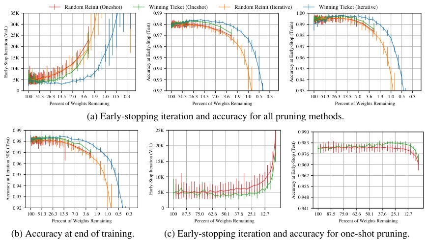
(a) Early-stopping iteration and accuracy for all pruning methods.

（a）所有剪枝方法下的早停迭代与精度。

3 Winning Tickets in Convolutional Networks

3 卷积网络中的中奖彩票

Here, we apply the lottery ticket hypothesis to convolutional networks on CIFAR10, increasing both the complexity of the learning problem and the size of the networks. We consider the Conv-2, Conv-4, and Conv-6 architectures in Figure 2, which are scaled-down variants of the VGG (Simonyan & Zisserman, 2014) family. The networks have two, four, or six convolutional layers followed by two fully-connected layers; max-pooling occurs after every two convolutional layers. The networks cover a range from near-fully-connected to traditional convolutional networks, with less than 1% of parameters in convolutional layers in Conv-2 to nearly two thirds in Conv-6.[^3]

这里，我们把彩票假设应用到 CIFAR10 上的卷积网络，同时提高学习问题的复杂度和网络规模。我们考虑图 2 中的 Conv-2、Conv-4 和 Conv-6 结构，它们是缩小版的 VGG 家族变体（Simonyan & Zisserman, 2014）。这些网络分别有两、四或六个卷积层，后接两个全连接层；每两个卷积层之后做一次最大池化。这些网络覆盖了从近乎全连接到传统卷积网络的范围：Conv-2 中不到 1% 的参数在卷积层，Conv-6 中则接近三分之二。[^3]

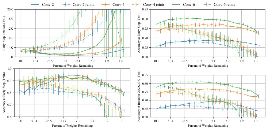
Figure 5: Early-stopping iteration and test and training accuracy of the Conv-2/4/6 architectures when iteratively pruned and when randomly reinitialized. Each solid line is the average of five trials; each dashed line is the average of fifteen reinitializations (three per trial). The bottom right graph plots test accuracy of winning tickets at iterations corresponding to the last iteration of training for the original network (20,000 for Conv-2, 25,000 for Conv-4, and 30,000 for Conv-6); at this iteration, training accuracy $\approx 100\%$ for $P_{m}\geq 2\%$ for winning tickets (see Appendix D).

图 5：Conv-2/4/6 结构在迭代剪枝和随机重新初始化时的早停迭代以及测试与训练精度。每条实线是五次试验的平均；每条虚线是十五次重新初始化的平均（每次试验三次）。右下图画出中奖彩票在对应原网络最后一次训练迭代（Conv-2 为 20,000，Conv-4 为 25,000，Conv-6 为 30,000）时的测试精度；在该迭代上，中奖彩票在 $P_{m}\geq 2\%$ 时训练精度 $\approx 100\%$（见附录 D）。

Finding winning tickets. The solid lines in Figure 5 (top) show the iterative lottery ticket experiment on Conv-2 (blue), Conv-4 (orange), and Conv-6 (green) at the per-layer pruning rates from Figure 2. The pattern from Lenet in Section 2 repeats: as the network is pruned, it learns faster and test accuracy rises as compared to the original network. In this case, the results are more pronounced. Winning tickets reach minimum validation loss at best 3.5x faster for Conv-2 ($P_{m}=8.8\%$), 3.5x for Conv-4 ($P_{m}=9.2\%$), and 2.5x for Conv-6 ($P_{m}=15.1\%$). Test accuracy improves at best 3.4 percentage points for Conv-2 ($P_{m}=4.6\%$), 3.5 for Conv-4 ($P_{m}=11.1\%$), and 3.3 for Conv-6 ($P_{m}=26.4\%$). All three networks remain above their original average test accuracy when $P_{m}>2\%$.

寻找中奖彩票。 图 5（上）中的实线展示了按图 2 中的逐层剪枝率，在 Conv-2（蓝）、Conv-4（橙）和 Conv-6（绿）上做的迭代彩票实验。第 2 节 Lenet 上的模式再次出现：随着网络被剪枝，它比原网络学得更快，测试精度也上升。这一次结果更明显。中奖彩票最快分别比原网络早 3.5 倍（Conv-2，$P_{m}=8.8\%$）、3.5 倍（Conv-4，$P_{m}=9.2\%$）和 2.5 倍（Conv-6，$P_{m}=15.1\%$）达到最低验证损失。测试精度最多分别提高 3.4 个百分点（Conv-2，$P_{m}=4.6\%$）、3.5（Conv-4，$P_{m}=11.1\%$）和 3.3（Conv-6，$P_{m}=26.4\%$）。当 $P_{m}>2\%$ 时，三个网络都保持在各自原来的平均测试精度之上。

As in Section 2, training accuracy at the early-stopping iteration rises with test accuracy. However, at iteration 20,000 for Conv-2, 25,000 for Conv-4, and 30,000 for Conv-6 (the iterations corresponding to the final training iteration for the original network), training accuracy reaches 100% for all networks when $P_{m}\geq 2\%$ (Appendix D, Figure 13) and winning tickets still maintain higher test accuracy (Figure 5 bottom right). This means that the gap between test and training accuracy is smaller for winning tickets, indicating they generalize better.

与第 2 节一样，早停迭代上的训练精度随测试精度一起上升。不过，在 Conv-2 的第 20,000 次、Conv-4 的第 25,000 次和 Conv-6 的第 30,000 次迭代（对应原网络最后一次训练迭代）时，所有网络在 $P_{m}\geq 2\%$ 时训练精度都达到 100%（附录 D，图 13），而中奖彩票仍然保持更高的测试精度（图 5 右下）。这意味着中奖彩票的测试与训练精度差距更小，表明它们泛化更好。

Random reinitialization. We repeat the random reinitialization experiment from Section 2, which appears as the dashed lines in Figure 5. These networks again take increasingly longer to learn upon continued pruning. Just as with Lenet on MNIST (Section 2), test accuracy drops off more quickly for the random reinitialization experiments. However, unlike Lenet, test accuracy at early-stopping time initially remains steady and even improves for Conv-2 and Conv-4, indicating that—at moderate levels of pruning—the structure of the winning tickets alone may lead to better accuracy.

随机重新初始化。 我们重复第 2 节的随机重新初始化实验，结果如图 5 中的虚线所示。这些网络在持续剪枝后又一次学得越来越慢。正如 MNIST 上的 Lenet（第 2 节），随机重新初始化实验的测试精度下降得更快。不过与 Lenet 不同，早停时的测试精度起初保持平稳，对 Conv-2 和 Conv-4 甚至有所提高，说明在中等程度的剪枝下，单靠中奖彩票的结构也可能带来更好的精度。

Dropout. Dropout (Srivastava et al., 2014; Hinton et al., 2012) improves accuracy by randomly disabling a fraction of the units (i.e., randomly sampling a subnetwork) on each training iteration. Baldi & Sadowski (2013) characterize dropout as simultaneously training the ensemble of all subnetworks. Since the lottery ticket hypothesis suggests that one of these subnetworks comprises a winning ticket, it is natural to ask whether dropout and our strategy for finding winning tickets interact.

Dropout。 Dropout（Srivastava et al., 2014; Hinton et al., 2012）通过在每次训练迭代中随机关闭一部分单元（也就是随机采样一个子网络）来提高精度。Baldi 与 Sadowski（2013）把 dropout 刻画为同时训练所有子网络组成的集成。既然彩票假设认为这些子网络中有一个构成中奖彩票，自然要问：dropout 与我们寻找中奖彩票的策略是否会相互作用。

Figure 6 shows the results of training Conv-2, Conv-4, and Conv-6 with a dropout rate of 0.5. Dashed lines are the network performance without dropout (the solid lines in Figure 5).[^4] We continue to find winning tickets when training with dropout. Dropout increases initial test accuracy (2.1, 3.0, and 2.4 percentage points on average for Conv-2, Conv-4, and Conv-6, respectively), and iterative pruning increases it further (up to an additional 2.3, 4.6, and 4.7 percentage points, respectively, on average). Learning becomes faster with iterative pruning as before, but less dramatically in the case of Conv-2.

图 6 展示了以 0.5 的 dropout 率训练 Conv-2、Conv-4 和 Conv-6 的结果。虚线是不使用 dropout 时的网络表现（图 5 中的实线）。[^4] 在使用 dropout 训练时，我们仍然能找到中奖彩票。Dropout 提高了初始测试精度（Conv-2、Conv-4 和 Conv-6 平均分别提高 2.1、3.0 和 2.4 个百分点），迭代剪枝则进一步提高（平均分别最多再提高 2.3、4.6 和 4.7 个百分点）。与之前一样，学习随迭代剪枝变快，但在 Conv-2 上不那么显著。

These improvements suggest that our iterative pruning strategy interacts with dropout in a complementary way. Srivastava et al. (2014) observe that dropout induces sparse activations in the final network; it is possible that dropout-induced sparsity primes a network to be pruned. If so, dropout techniques that target weights (Wan et al., 2013) or learn per-weight dropout probabilities (Molchanov et al., 2017; Louizos et al., 2018) could make winning tickets even easier to find.

这些改进表明，我们的迭代剪枝策略与 dropout 以互补的方式相互作用。Srivastava 等人（2014）观察到，dropout 会在最终网络中诱导稀疏激活；有可能由 dropout 诱导的稀疏性为网络被剪枝做好了准备。若果真如此，针对权重的 dropout 技术（Wan et al., 2013）或学习每个权重 dropout 概率的技术（Molchanov et al., 2017; Louizos et al., 2018）可能会让中奖彩票更容易找到。

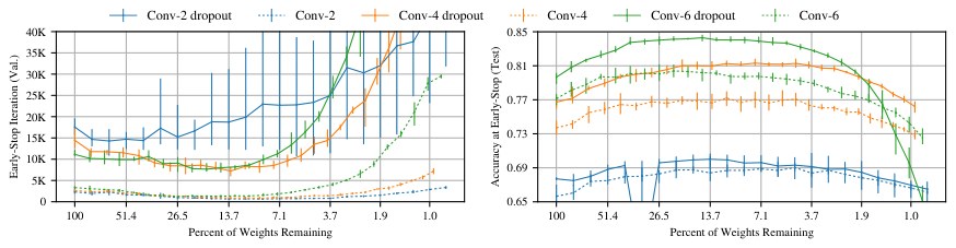
Figure 6: Early-stopping iteration and test accuracy at early-stopping of Conv-2/4/6 when iteratively pruned and trained with dropout. The dashed lines are the same networks trained without dropout (the solid lines in Figure 5). Learning rates are 0.0003 for Conv-2 and 0.0002 for Conv-4 and Conv-6.

图 6：Conv-2/4/6 在迭代剪枝并用 dropout 训练时的早停迭代以及早停时的测试精度。虚线是不使用 dropout 训练的同一批网络（图 5 中的实线）。学习率对 Conv-2 为 0.0003，对 Conv-4 和 Conv-6 为 0.0002。

4 VGG and Resnet for CIFAR10

4 用于 CIFAR10 的 VGG 与 Resnet

Here, we study the lottery ticket hypothesis on networks evocative of the architectures and techniques used in practice. Specifically, we consider VGG-style deep convolutional networks (VGG-19 on CIFAR10—Simonyan & Zisserman (2014)) and residual networks (Resnet-18 on CIFAR10—He et al. (2016)).[^5] These networks are trained with batchnorm, weight decay, decreasing learning rate schedules, and augmented training data. We continue to find winning tickets for all of these architectures; however, our method for finding them, iterative pruning, is sensitive to the particular learning rate used. In these experiments, rather than measure early-stopping time (which, for these larger networks, is entangled with learning rate schedules), we plot accuracy at several moments during training to illustrate the relative rates at which accuracy improves.

这里，我们在更接近实践中所用结构和技术的网络上研究彩票假设。具体来说，我们考虑 VGG 风格的深度卷积网络（CIFAR10 上的 VGG-19——Simonyan & Zisserman（2014））以及残差网络（CIFAR10 上的 Resnet-18——He 等人（2016））。[^5] 这些网络使用批归一化、权重衰减、递减的学习率调度以及增强后的训练数据来训练。我们仍然在所有这些结构中找到了中奖彩票；不过，我们寻找它们的方法——迭代剪枝——对所用的具体学习率敏感。在这些实验中，我们不再测量早停时间（对更大的网络而言，它与学习率调度缠在一起），而是画出训练过程中若干时刻的精度，以说明精度相对提升的速率。

Global pruning. On Lenet and Conv-2/4/6, we prune each layer separately at the same rate. For Resnet-18 and VGG-19, we modify this strategy slightly: we prune these deeper networks globally, removing the lowest-magnitude weights collectively across all convolutional layers. In Appendix I.1, we find that global pruning identifies smaller winning tickets for Resnet-18 and VGG-19. Our conjectured explanation for this behavior is as follows: For these deeper networks, some layers have far more parameters than others. For example, the first two convolutional layers of VGG-19 have 1728 and 36864 parameters, while the last has 2.35 million. When all layers are pruned at the same rate, these smaller layers become bottlenecks, preventing us from identifying the smallest possible winning tickets. Global pruning makes it possible to avoid this pitfall.

全局剪枝。 在 Lenet 和 Conv-2/4/6 上，我们以相同比率分别对每一层剪枝。对 Resnet-18 和 VGG-19，我们略微修改这一策略：对这些更深的网络做全局剪枝，在所有卷积层中集体去掉幅度最低的权重。在附录 I.1 中，我们发现全局剪枝能为 Resnet-18 和 VGG-19 识别出更小的中奖彩票。我们对这一行为的猜想解释如下：对这些更深的网络，有些层的参数远多于其他层。例如，VGG-19 的前两个卷积层分别有 1728 和 36864 个参数，而最后一层有 235 万。当所有层以相同比率剪枝时，这些更小的层会成为瓶颈，使我们无法识别尽可能小的中奖彩票。全局剪枝使得有可能避开这一陷阱。

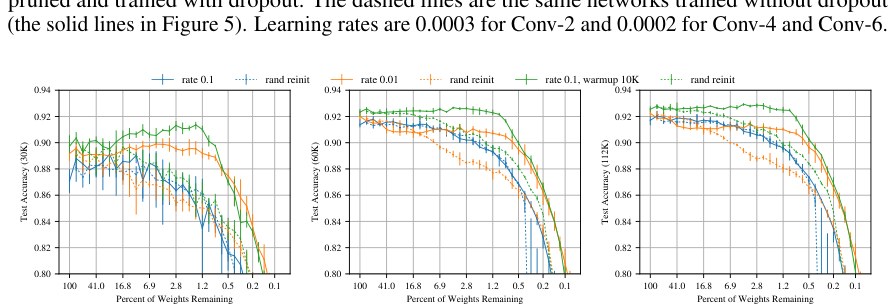
Figure 7: Test accuracy (at 30K, 60K, and 112K iterations) of VGG-19 when iteratively pruned.

图 7：VGG-19 在迭代剪枝时（于 30K、60K 和 112K 次迭代）的测试精度。

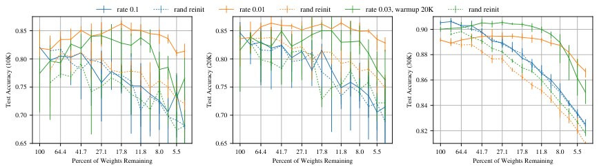
Figure 8: Test accuracy (at 10K, 20K, and 30K iterations) of Resnet-18 when iteratively pruned.

图 8：Resnet-18 在迭代剪枝时（于 10K、20K 和 30K 次迭代）的测试精度。

VGG-19. We study the variant VGG-19 adapted for CIFAR10 by Liu et al. (2019); we use the the same training regime and hyperparameters: 160 epochs (112,480 iterations) with SGD with momentum (0.9) and decreasing the learning rate by a factor of 10 at 80 and 120 epochs. This network has 20 million parameters. Figure 7 shows the results of iterative pruning and random reinitialization on VGG-19 at two initial learning rates: 0.1 (used in Liu et al. (2019)) and 0.01. At the higher learning rate, iterative pruning does not find winning tickets, and performance is no better than when the pruned networks are randomly reinitialized. However, at the lower learning rate, the usual pattern reemerges, with subnetworks that remain within 1 percentage point of the original accuracy while $P_{m}\geq 3.5\%$. (They are not winning tickets, since they do not match the original accuracy.) When randomly reinitialized, the subnetworks lose accuracy as they are pruned in the same manner as other experiments throughout this paper. Although these subnetworks learn faster than the unpruned network early in training (Figure 7 left), this accuracy advantage erodes later in training due to the lower initial learning rate. However, these subnetworks still learn faster than when reinitialized.

VGG-19。 我们研究 Liu 等人（2019）为 CIFAR10 改编的 VGG-19 变体；我们使用相同的训练制度与超参数：160 个周期（112,480 次迭代），用带动量（0.9）的 SGD，并在第 80 和 120 个周期把学习率降为原来的十分之一。该网络有 2000 万参数。图 7 展示了 VGG-19 在两种初始学习率下迭代剪枝和随机重新初始化的结果：0.1（Liu 等人（2019）所用）和 0.01。在较高学习率下，迭代剪枝找不到中奖彩票，表现并不好于把剪枝后的网络随机重新初始化。然而在较低学习率下，通常的模式再次出现：当 $P_{m}\geq 3.5\%$ 时，子网络保持在原精度的 1 个百分点以内。（它们还不算中奖彩票，因为没有匹配原精度。）随机重新初始化时，这些子网络随着被剪枝而损失精度，方式与本文其他实验相同。尽管这些子网络在训练早期比未剪枝网络学得更快（图 7 左），由于初始学习率较低，这一精度优势在训练后期会被侵蚀。不过，这些子网络仍然比重新初始化时学得更快。

To bridge the gap between the lottery ticket behavior of the lower learning rate and the accuracy advantage of the higher learning rate, we explore the effect of linear learning rate warmup from 0 to the initial learning rate over $k$ iterations. Training VGG-19 with warmup ($k=10000$, green line) at learning rate 0.1 improves the test accuracy of the unpruned network by about one percentage point. Warmup makes it possible to find winning tickets, exceeding this initial accuracy when $P_{m}\geq 1.5\%$.

为了弥合较低学习率下的彩票行为与较高学习率下的精度优势之间的差距，我们考察在 $k$ 次迭代内把学习率从 0 线性预热到初始学习率的效果。用预热（$k=10000$，绿线）以学习率 0.1 训练 VGG-19，使未剪枝网络的测试精度大约提高一个百分点。预热使得能够找到中奖彩票，当 $P_{m}\geq 1.5\%$ 时超过这一初始精度。

Resnet-18. Resnet-18 (He et al., 2016) is a 20 layer convolutional network with residual connections designed for CIFAR10. It has 271,000 parameters. We train the network for 30,000 iterations with SGD with momentum (0.9), decreasing the learning rate by a factor of 10 at 20,000 and 25,000 iterations. Figure 8 shows the results of iterative pruning and random reinitialization at learning rates 0.1 (used in He et al. (2016)) and 0.01. These results largely mirror those of VGG: iterative pruning finds winning tickets at the lower learning rate but not the higher learning rate. The accuracy of the best winning tickets at the lower learning rate (89.5% when $41.7\%\geq P_{m}\geq 21.9\%$) falls short of the original network’s accuracy at the higher learning rate (90.5%). At lower learning rate, the winning ticket again initially learns faster (left plots of Figure 8), but falls behind the unpruned network at the higher learning rate later in training (right plot). Winning tickets trained with warmup close the accuracy gap with the unpruned network at the higher learning rate, reaching 90.5% test accuracy with learning rate 0.03 (warmup, $k=20000$) at $P_{m}=27.1\%$. For these hyperparameters, we still find winning tickets when $P_{m}\geq 11.8\%$. Even with warmup, however, we could not find hyperparameters for which we could identify winning tickets at the original learning rate, 0.1.

Resnet-18。 Resnet-18（He et al., 2016）是一个为 CIFAR10 设计的 20 层卷积网络，带有残差连接。它有 271,000 个参数。我们用带动量（0.9）的 SGD 训练网络 30,000 次迭代，并在第 20,000 和 25,000 次迭代把学习率降为原来的十分之一。图 8 展示了学习率为 0.1（He 等人（2016）所用）和 0.01 时迭代剪枝与随机重新初始化的结果。这些结果大体上映射了 VGG 的情况：迭代剪枝在较低学习率下找到中奖彩票，在较高学习率下则找不到。较低学习率下最好的中奖彩票精度（当 $41.7\%\geq P_{m}\geq 21.9\%$ 时为 89.5%）达不到原网络在较高学习率下的精度（90.5%）。在较低学习率下，中奖彩票起初学得更快（图 8 左图），但在训练后期落后于较高学习率下的未剪枝网络（右图）。用预热训练的中奖彩票缩小了与较高学习率下未剪枝网络的精度差距：在学习率 0.03（预热，$k=20000$）、$P_{m}=27.1\%$ 时达到 90.5% 测试精度。对这些超参数，当 $P_{m}\geq 11.8\%$ 时我们仍然能找到中奖彩票。即便使用预热，我们也未能找到一组超参数，能在原来的学习率 0.1 下识别出中奖彩票。

5 Discussion

5 讨论

Existing work on neural network pruning (e.g., Han et al. (2015)) demonstrates that the function learned by a neural network can often be represented with fewer parameters. Pruning typically proceeds by training the original network, removing connections, and further fine-tuning. In effect, the initial training initializes the weights of the pruned network so that it can learn in isolation during fine-tuning. We seek to determine if similarly sparse networks can learn from the start. We find that the architectures studied in this paper reliably contain such trainable subnetworks, and the lottery ticket hypothesis proposes that this property applies in general. Our empirical study of the existence and nature of winning tickets invites a number of follow-up questions.

已有的神经网络剪枝工作（例如 Han 等人（2015））表明，神经网络学到的函数往往可以用更少的参数来表示。剪枝通常的流程是：训练原网络，去掉连接，再进一步微调。实际上，最初的训练为剪枝后的网络初始化了权重，使它能在微调期间单独学习。我们想确定，类似稀疏的网络是否从一开始就能学习。我们发现，本文研究的结构可靠地包含这类可训练子网络，而彩票假设提出这一性质普遍成立。我们对中奖彩票之存在与性质的经验研究，引出了若干后续问题。

The importance of winning ticket initialization. When randomly reinitialized, a winning ticket learns more slowly and achieves lower test accuracy, suggesting that initialization is important to its success. One possible explanation for this behavior is these initial weights are close to their final values after training—that in the most extreme case, they are already trained. However, experiments in Appendix F show the opposite—that the winning ticket weights move further than other weights. This suggests that the benefit of the initialization is connected to the optimization algorithm, dataset, and model. For example, the winning ticket initialization might land in a region of the loss landscape that is particularly amenable to optimization by the chosen optimization algorithm.

中奖彩票初始化的重要性。 随机重新初始化后，中奖彩票学得更慢、测试精度更低，说明初始化对其成功很重要。对这一行为的一种可能解释是：这些初始权重已经接近训练后的最终取值——在最极端的情形下，它们已经被训练好了。然而附录 F 中的实验表明情况恰恰相反——中奖彩票的权重要比其他权重移动得更远。这说明初始化的好处与优化算法、数据集和模型相关。例如，中奖彩票的初始化可能落在损失地形中特别便于所选优化算法进行优化的区域。

Liu et al. (2019) find that pruned networks are indeed trainable when randomly reinitialized, seemingly contradicting conventional wisdom and our random reinitialization experiments. For example, on VGG-19 (for which we share the same setup), they find that networks pruned by up to 80% and randomly reinitialized match the accuracy of the original network. Our experiments in Figure 7 confirm these findings at this level of sparsity (below which Liu et al. do not present data). However, after further pruning, initialization matters: we find winning tickets when VGG-19 is pruned by up to 98.5%; when reinitialized, these tickets reach much lower accuracy. We hypothesize that—up to a certain level of sparsity—highly overparameterized networks can be pruned, reinitialized, and retrained successfully; however, beyond this point, extremely pruned, less severely overparamterized networks only maintain accuracy with fortuitous initialization.

Liu 等人（2019）发现，剪枝后的网络在随机重新初始化后确实可训练，这似乎与传统看法以及我们的随机重新初始化实验相矛盾。例如，在 VGG-19 上（我们使用相同的设置），他们发现剪掉最多 80% 并随机重新初始化的网络能够匹配原网络的精度。我们在图 7 中的实验在这一稀疏程度上确认了这些发现（在此之下 Liu 等人没有给出数据）。然而在进一步剪枝之后，初始化就变得重要：当 VGG-19 被剪掉最多 98.5% 时，我们找到了中奖彩票；重新初始化后，这些彩票达到的精度低得多。我们猜想：在某种稀疏程度之内，高度过参数化的网络可以被剪枝、重新初始化并成功重新训练；超过这一点，被极度剪枝、过参数化不那么严重的网络只有带着幸运的初始化才能保持精度。

The importance of winning ticket structure. The initialization that gives rise to a winning ticket is arranged in a particular sparse architecture. Since we uncover winning tickets through heavy use of training data, we hypothesize that the structure of our winning tickets encodes an inductive bias customized to the learning task at hand. Cohen & Shashua (2016) show that the inductive bias embedded in the structure of a deep network determines the kinds of data that it can separate more parameter-efficiently than can a shallow network; although Cohen & Shashua (2016) focus on the pooling geometry of convolutional networks, a similar effect may be at play with the structure of winning tickets, allowing them to learn even when heavily pruned.

中奖彩票结构的重要性。 产生中奖彩票的初始化被安排在一种特定的稀疏结构中。由于我们通过大量使用训练数据来揭示中奖彩票，我们猜想中奖彩票的结构编码了一种针对手头学习任务定制的归纳偏置。Cohen 与 Shashua（2016）表明，深网络结构中嵌入的归纳偏置决定了它能以比浅网络更参数高效的方式分开哪类数据；尽管 Cohen 与 Shashua（2016）关注的是卷积网络的池化几何，类似的效应也可能出现在中奖彩票的结构中，使它们即使被重度剪枝仍然能够学习。

The improved generalization of winning tickets. We reliably find winning tickets that generalize better, exceeding the test accuracy of the original network while matching its training accuracy. Test accuracy increases and then decreases as we prune, forming an Occam’s Hill  (Rasmussen & Ghahramani, 2001) where the original, overparameterized model has too much complexity (perhaps overfitting) and the extremely pruned model has too little. The conventional view of the relationship between compression and generalization is that compact hypotheses can better generalize (Rissanen, 1986). Recent theoretical work shows a similar link for neural networks, proving tighter generalization bounds for networks that can be compressed further (Zhou et al. (2018) for pruning/quantization and Arora et al. (2018) for noise robustness). The lottery ticket hypothesis offers a complementary perspective on this relationship—that larger networks might explicitly contain simpler representations.

中奖彩票更好的泛化。 我们可靠地找到泛化更好的中奖彩票：它们在匹配原网络训练精度的同时超过其测试精度。随着我们剪枝，测试精度先升后降，形成一个奥卡姆之丘（Occam's Hill）（Rasmussen & Ghahramani, 2001）：原来过参数化的模型复杂度过高（或许过拟合），而被极度剪枝的模型复杂度又过低。关于压缩与泛化关系的传统看法是，紧凑的假设能更好地泛化（Rissanen, 1986）。近期理论工作为神经网络展示了类似的联系，证明能被进一步压缩的网络有更紧的泛化界（Zhou 等人（2018）针对剪枝/量化，Arora 等人（2018）针对噪声稳健性）。彩票假设为这一关系提供了一个互补视角——更大的网络可能显式地包含更简单的表示。

Implications for neural network optimization. Winning tickets can reach accuracy equivalent to that of the original, unpruned network, but with significantly fewer parameters. This observation connects to recent work on the role of overparameterization in neural network training. For example, Du et al. (2019) prove that sufficiently overparameterized two-layer relu networks (with fixed-size second layers) trained with SGD converge to global optima. A key question, then, is whether the presence of a winning ticket is necessary or sufficient for SGD to optimize a neural network to a particular test accuracy. We conjecture (but do not empirically show) that SGD seeks out and trains a well-initialized subnetwork. By this logic, overparameterized networks are easier to train because they have more combinations of subnetworks that are potential winning tickets.

对神经网络优化的含义。 中奖彩票能够达到与原来未剪枝网络相当的精度，但参数显著更少。这一观察与近期关于过参数化在神经网络训练中作用的工作相联系。例如，Du 等人（2019）证明，充分过参数化的两层 relu 网络（第二层大小固定）用 SGD 训练时会收敛到全局最优。于是一个关键问题是：中奖彩票的存在，对于 SGD 把神经网络优化到特定测试精度而言，究竟是必要的还是充分的。我们猜想（但并未从经验上表明）：SGD 会寻找并训练一个初始化良好的子网络。按此逻辑，过参数化网络更容易训练，是因为它们拥有更多可能成为中奖彩票的子网络组合。

6 Limitations and Future Work

6 局限与未来工作

We only consider vision-centric classification tasks on smaller datasets (MNIST, CIFAR10). We do not investigate larger datasets (namely Imagenet (Russakovsky et al., 2015)): iterative pruning is computationally intensive, requiring training a network 15 or more times consecutively for multiple trials. In future work, we intend to explore more efficient methods for finding winning tickets that will make it possible to study the lottery ticket hypothesis in more resource-intensive settings.

我们只考虑较小数据集（MNIST、CIFAR10）上以视觉为中心的分类任务。我们没有研究更大的数据集（主要是 Imagenet（Russakovsky et al., 2015））：迭代剪枝在计算上很密集，需要把一个网络连续训练 15 次或更多，并做多次试验。在未来工作中，我们打算探索更高效的寻找中奖彩票的方法，以便在更耗费资源的设置中研究彩票假设。

Sparse pruning is our only method for finding winning tickets. Although we reduce parameter-counts, the resulting architectures are not optimized for modern libraries or hardware. In future work, we intend to study other pruning methods from the extensive contemporary literature, such as structured pruning (which would produce networks optimized for contemporary hardware) and non-magnitude pruning methods (which could produce smaller winning tickets or find them earlier).

稀疏剪枝是我们寻找中奖彩票的唯一方法。尽管我们减少了参数量，得到的结构并未针对现代库或硬件做优化。在未来工作中，我们打算研究当代大量文献中的其他剪枝方法，例如结构化剪枝（会产生针对当代硬件优化的网络）以及非基于幅度的剪枝方法（可能产生更小的中奖彩票，或更早找到它们）。

The winning tickets we find have initializations that allow them to match the performance of the unpruned networks at sizes too small for randomly-initialized networks to do the same. In future work, we intend to study the properties of these initializations that, in concert with the inductive biases of the pruned network architectures, make these networks particularly adept at learning.

我们找到的中奖彩票拥有这样的初始化：它们能在随机初始化网络已无法做到的过小规模上，匹配未剪枝网络的表现。在未来工作中，我们打算研究这些初始化的性质：它们与被剪枝网络结构的归纳偏置一起，使这些网络特别擅长学习。

On deeper networks (Resnet-18 and VGG-19), iterative pruning is unable to find winning tickets unless we train the networks with learning rate warmup. In future work, we plan to explore why warmup is necessary and whether other improvements to our scheme for identifying winning tickets could obviate the need for these hyperparameter modifications.

在更深的网络（Resnet-18 和 VGG-19）上，除非我们用学习率预热来训练网络，否则迭代剪枝无法找到中奖彩票。在未来工作中，我们计划探索为何预热是必要的，以及对识别中奖彩票之方案的其他改进是否能省去这些超参数修改。

7 Related Work

7 相关工作

In practice, neural networks tend to be dramatically overparameterized. Distillation (Ba & Caruana, 2014; Hinton et al., 2015) and pruning (LeCun et al., 1990; Han et al., 2015) rely on the fact that parameters can be reduced while preserving accuracy. Even with sufficient capacity to memorize training data, networks naturally learn simpler functions (Zhang et al., 2016; Neyshabur et al., 2014; Arpit et al., 2017). Contemporary experience (Bengio et al., 2006; Hinton et al., 2015; Zhang et al., 2016) and Figure 1 suggest that overparameterized networks are easier to train. We show that dense networks contain sparse subnetworks capable of learning on their own starting from their original initializations. Several other research directions aim to train small or sparse networks.

实践中，神经网络往往被极大地过参数化。蒸馏（Ba & Caruana, 2014; Hinton et al., 2015）和剪枝（LeCun et al., 1990; Han et al., 2015）都依赖于这样一个事实：可以在保持精度的同时减少参数。即便有足够容量记住训练数据，网络也会自然地学习更简单的函数（Zhang et al., 2016; Neyshabur et al., 2014; Arpit et al., 2017）。当代经验（Bengio et al., 2006; Hinton et al., 2015; Zhang et al., 2016）以及图 1 表明，过参数化网络更容易训练。我们表明，稠密网络中包含稀疏子网络，它们从原来的初始化出发就能独自学习。另外几个研究方向旨在训练小型或稀疏网络。

Prior to training. Squeezenet (Iandola et al., 2016) and MobileNets (Howard et al., 2017) are specifically engineered image-recognition networks that are an order of magnitude smaller than standard architectures. Denil et al. (2013) represent weight matrices as products of lower-rank factors. Li et al. (2018) restrict optimization to a small, randomly-sampled subspace of the parameter space (meaning all parameters can still be updated); they successfully train networks under this restriction. We show that one need not even update all parameters to optimize a network, and we find winning tickets through a principled search process involving pruning. Our contribution to this class of approaches is to demonstrate that sparse, trainable networks exist within larger networks.

训练之前。 Squeezenet（Iandola et al., 2016）和 MobileNets（Howard et al., 2017）是专门设计的图像识别网络，比标准结构小一个数量级。Denil 等人（2013）把权重矩阵表示为更低秩因子的乘积。Li 等人（2018）把优化限制在参数空间中一个随机采样的小子空间内（这意味着所有参数仍可更新）；他们在这一限制下成功训练了网络。我们表明，甚至不必更新所有参数就能优化一个网络，并且我们通过一个涉及剪枝的有原则搜索过程来寻找中奖彩票。我们对这类方法的贡献是表明：更大的网络内部存在着稀疏、可训练的网络。

After training. Distillation (Ba & Caruana, 2014; Hinton et al., 2015) trains small networks to mimic the behavior of large networks; small networks are easier to train in this paradigm. Recent pruning work compresses large models to run with limited resources (e.g., on mobile devices). Although pruning is central to our experiments, we study why training needs the overparameterized networks that make pruning possible. LeCun et al. (1990) and Hassibi & Stork (1993) first explored pruning based on second derivatives. More recently, Han et al. (2015) showed per-weight magnitude-based pruning substantially reduces the size of image-recognition networks. Guo et al. (2016) restore pruned connections as they become relevant again. Han et al. (2017) and Jin et al. (2016) restore pruned connections to increase network capacity after small weights have been pruned and surviving weights fine-tuned. Other proposed pruning heuristics include pruning based on activations (Hu et al., 2016), redundancy (Mariet & Sra, 2016; Srinivas & Babu, 2015a), per-layer second derivatives (Dong et al., 2017), and energy/computation efficiency (Yang et al., 2017) (e.g., pruning convolutional filters (Li et al., 2016; Molchanov et al., 2016; Luo et al., 2017) or channels (He et al., 2017)). Cohen et al. (2016) observe that convolutional filters are sensitive to initialization (“The Filter Lottery”); throughout training, they randomly reinitialize unimportant filters.

训练之后。 蒸馏（Ba & Caruana, 2014; Hinton et al., 2015）训练小网络去模仿大网络的行为；在这一范式下小网络更容易训练。近期的剪枝工作压缩大模型，以便在资源有限的条件下运行（例如在移动设备上）。尽管剪枝是我们实验的核心，我们研究的是：训练为何需要那些使剪枝成为可能的过参数化网络。LeCun 等人（1990）和 Hassibi 与 Stork（1993）最先探索了基于二阶导的剪枝。更近一些，Han 等人（2015）表明逐权重、基于幅度的剪枝能显著减小图像识别网络的规模。Guo 等人（2016）在被剪掉的连接再次变得相关时把它们恢复。Han 等人（2017）和 Jin 等人（2016）在小权重被剪掉、存活权重经过微调之后，恢复被剪掉的连接以增加网络容量。其他已提出的剪枝启发式包括基于激活的剪枝（Hu et al., 2016）、基于冗余的剪枝（Mariet & Sra, 2016; Srinivas & Babu, 2015a）、基于逐层二阶导的剪枝（Dong et al., 2017），以及基于能量/计算效率的剪枝（Yang et al., 2017）（例如剪掉卷积滤波器（Li et al., 2016; Molchanov et al., 2016; Luo et al., 2017）或通道（He et al., 2017））。Cohen 等人（2016）观察到卷积滤波器对初始化敏感（“滤波器彩票”）；在整个训练过程中，他们随机重新初始化不重要的滤波器。

During training. Bellec et al. (2018) train with sparse networks and replace weights that reach zero with new random connections. Srinivas et al. (2017) and Louizos et al. (2018) learn gating variables that minimize the number of nonzero parameters. Narang et al. (2017) integrate magnitude-based pruning into training. Gal & Ghahramani (2016) show that dropout approximates Bayesian inference in Gaussian processes. Bayesian perspectives on dropout learn dropout probabilities during training (Gal et al., 2017; Kingma et al., 2015; Srinivas & Babu, 2016). Techniques that learn per-weight, per-unit (Srinivas & Babu, 2016), or structured dropout probabilities naturally (Molchanov et al., 2017; Neklyudov et al., 2017) or explicitly (Louizos et al., 2017; Srinivas & Babu, 2015b) prune and sparsify networks during training as dropout probabilities for some weights reach 1. In contrast, we train networks at least once to find winning tickets. These techniques might also find winning tickets, or, by inducing sparsity, might beneficially interact with our methods.

训练期间。 Bellec 等人（2018）用稀疏网络训练，并把达到零的权重替换成新的随机连接。Srinivas 等人（2017）和 Louizos 等人（2018）学习用于最小化非零参数数量的门控变量。Narang 等人（2017）把基于幅度的剪枝整合进训练。Gal 与 Ghahramani（2016）表明，dropout 近似高斯过程中的贝叶斯推断。关于 dropout 的贝叶斯视角在训练期间学习 dropout 概率（Gal et al., 2017; Kingma et al., 2015; Srinivas & Babu, 2016）。学习每个权重、每个单元（Srinivas & Babu, 2016）或结构化 dropout 概率的技术，会在某些权重的 dropout 概率达到 1 时，自然地（Molchanov et al., 2017; Neklyudov et al., 2017）或显式地（Louizos et al., 2017; Srinivas & Babu, 2015b）在训练期间对网络剪枝并使其稀疏。相比之下，我们至少把网络训练一次来寻找中奖彩票。这些技术也可能找到中奖彩票，或者通过诱导稀疏性，与我们的方法产生有益的相互作用。

References

参考文献

Arora et al. (2018) Sanjeev Arora, Rong Ge, Behnam Neyshabur, and Yi Zhang. Stronger generalization bounds for deep nets via a compression approach. ICML , 2018.

Arpit et al. (2017) Devansh Arpit, Stanisław Jastrzębski, Nicolas Ballas, David Krueger, Emmanuel Bengio, Maxinder S Kanwal, Tegan Maharaj, Asja Fischer, Aaron Courville, Yoshua Bengio, et al. A closer look at memorization in deep networks. In International Conference on Machine Learning , pp. 233–242, 2017.

Ba & Caruana (2014) Jimmy Ba and Rich Caruana. Do deep nets really need to be deep? In Advances in neural information processing systems , pp. 2654–2662, 2014.

Baldi & Sadowski (2013) Pierre Baldi and Peter J Sadowski. Understanding dropout. In Advances in neural information processing systems , pp. 2814–2822, 2013.

Bellec et al. (2018) Guillaume Bellec, David Kappel, Wolfgang Maass, and Robert Legenstein. Deep rewiring: Training very sparse deep networks. Proceedings of ICLR , 2018.

Bengio et al. (2006) Yoshua Bengio, Nicolas L Roux, Pascal Vincent, Olivier Delalleau, and Patrice Marcotte. Convex neural networks. In Advances in neural information processing systems , pp. 123–130, 2006.

Cohen et al. (2016) Joseph Paul Cohen, Henry Z Lo, and Wei Ding. Randomout: Using a convolutional gradient norm to win the filter lottery. ICLR Workshop , 2016.

Cohen & Shashua (2016) Nadav Cohen and Amnon Shashua. Inductive bias of deep convolutional networks through pooling geometry. arXiv preprint arXiv:1605.06743 , 2016.

Denil et al. (2013) Misha Denil, Babak Shakibi, Laurent Dinh, Nando De Freitas, et al. Predicting parameters in deep learning. In Advances in neural information processing systems , pp. 2148–2156, 2013.

Dong et al. (2017) Xin Dong, Shangyu Chen, and Sinno Pan. Learning to prune deep neural networks via layer-wise optimal brain surgeon. In Advances in Neural Information Processing Systems , pp. 4860–4874, 2017.

Du et al. (2019) Simon S. Du, Xiyu Zhai, Barnabas Poczos, and Aarti Singh. Gradient descent provably optimizes over-parameterized neural networks. In International Conference on Learning Representations , 2019. URL https://openreview.net/forum?id=S1eK3i09YQ .

Gal & Ghahramani (2016) Yarin Gal and Zoubin Ghahramani. Dropout as a bayesian approximation: Representing model uncertainty in deep learning. In international conference on machine learning , pp. 1050–1059, 2016.

Gal et al. (2017) Yarin Gal, Jiri Hron, and Alex Kendall. Concrete dropout. In Advances in Neural Information Processing Systems , pp. 3584–3593, 2017.

Glorot & Bengio (2010) Xavier Glorot and Yoshua Bengio. Understanding the difficulty of training deep feedforward neural networks. In Proceedings of the thirteenth international conference on artificial intelligence and statistics , pp. 249–256, 2010.

Guo et al. (2016) Yiwen Guo, Anbang Yao, and Yurong Chen. Dynamic network surgery for efficient dnns. In Advances In Neural Information Processing Systems , pp. 1379–1387, 2016.

Han et al. (2015) Song Han, Jeff Pool, John Tran, and William Dally. Learning both weights and connections for efficient neural network. In Advances in neural information processing systems , pp. 1135–1143, 2015.

Han et al. (2017) Song Han, Jeff Pool, Sharan Narang, Huizi Mao, Shijian Tang, Erich Elsen, Bryan Catanzaro, John Tran, and William J Dally. Dsd: Regularizing deep neural networks with dense-sparse-dense training flow. Proceedings of ICLR , 2017.

Hassibi & Stork (1993) Babak Hassibi and David G Stork. Second order derivatives for network pruning: Optimal brain surgeon. In Advances in neural information processing systems , pp. 164–171, 1993.

He et al. (2016) Kaiming He, Xiangyu Zhang, Shaoqing Ren, and Jian Sun. Deep residual learning for image recognition. In Proceedings of the IEEE conference on computer vision and pattern recognition , pp. 770–778, 2016.

He et al. (2017) Yihui He, Xiangyu Zhang, and Jian Sun. Channel pruning for accelerating very deep neural networks. In International Conference on Computer Vision (ICCV) , volume 2, pp.  6, 2017.

Hinton et al. (2015) Geoffrey Hinton, Oriol Vinyals, and Jeff Dean. Distilling the knowledge in a neural network. arXiv preprint arXiv:1503.02531 , 2015.

Hinton et al. (2012) Geoffrey E Hinton, Nitish Srivastava, Alex Krizhevsky, Ilya Sutskever, and Ruslan R Salakhutdinov. Improving neural networks by preventing co-adaptation of feature detectors. arXiv preprint arXiv:1207.0580 , 2012.

Howard et al. (2017) Andrew G Howard, Menglong Zhu, Bo Chen, Dmitry Kalenichenko, Weijun Wang, Tobias Weyand, Marco Andreetto, and Hartwig Adam. Mobilenets: Efficient convolutional neural networks for mobile vision applications. arXiv preprint arXiv:1704.04861 , 2017.

Hu et al. (2016) Hengyuan Hu, Rui Peng, Yu-Wing Tai, and Chi-Keung Tang. Network trimming: A data-driven neuron pruning approach towards efficient deep architectures. arXiv preprint arXiv:1607.03250 , 2016.

Iandola et al. (2016) Forrest N Iandola, Song Han, Matthew W Moskewicz, Khalid Ashraf, William J Dally, and Kurt Keutzer. Squeezenet: Alexnet-level accuracy with 50x fewer parameters and< 0.5 mb model size. arXiv preprint arXiv:1602.07360 , 2016.

Jin et al. (2016) Xiaojie Jin, Xiaotong Yuan, Jiashi Feng, and Shuicheng Yan. Training skinny deep neural networks with iterative hard thresholding methods. arXiv preprint arXiv:1607.05423 , 2016.

Kingma & Ba (2014) Diederik P Kingma and Jimmy Ba. Adam: A method for stochastic optimization. arXiv preprint arXiv:1412.6980 , 2014.

Kingma et al. (2015) Diederik P Kingma, Tim Salimans, and Max Welling. Variational dropout and the local reparameterization trick. In Advances in Neural Information Processing Systems , pp. 2575–2583, 2015.

Krizhevsky & Hinton (2009) Alex Krizhevsky and Geoffrey Hinton. Learning multiple layers of features from tiny images. 2009.

LeCun et al. (1990) Yann LeCun, John S Denker, and Sara A Solla. Optimal brain damage. In Advances in neural information processing systems , pp. 598–605, 1990.

LeCun et al. (1998) Yann LeCun, Léon Bottou, Yoshua Bengio, and Patrick Haffner. Gradient-based learning applied to document recognition. Proceedings of the IEEE , 86(11):2278–2324, 1998.

Li et al. (2018) Chunyuan Li, Heerad Farkhoor, Rosanne Liu, and Jason Yosinski. Measuring the intrinsic dimension of objective landscapes. Proceedings of ICLR , 2018.

Li et al. (2016) Hao Li, Asim Kadav, Igor Durdanovic, Hanan Samet, and Hans Peter Graf. Pruning filters for efficient convnets. arXiv preprint arXiv:1608.08710 , 2016.

Liu et al. (2019) Zhuang Liu, Mingjie Sun, Tinghui Zhou, Gao Huang, and Trevor Darrell. Rethinking the value of network pruning. In International Conference on Learning Representations , 2019. URL https://openreview.net/forum?id=rJlnB3C5Ym .

Louizos et al. (2017) Christos Louizos, Karen Ullrich, and Max Welling. Bayesian compression for deep learning. In Advances in Neural Information Processing Systems , pp. 3290–3300, 2017.

Louizos et al. (2018) Christos Louizos, Max Welling, and Diederik P Kingma. Learning sparse neural networks through l ​ _ ​ 0 l_0 regularization. Proceedings of ICLR , 2018.

Luo et al. (2017) Jian-Hao Luo, Jianxin Wu, and Weiyao Lin. Thinet: A filter level pruning method for deep neural network compression. arXiv preprint arXiv:1707.06342 , 2017.

Mariet & Sra (2016) Zelda Mariet and Suvrit Sra. Diversity networks. Proceedings of ICLR , 2016.

Molchanov et al. (2017) Dmitry Molchanov, Arsenii Ashukha, and Dmitry Vetrov. Variational dropout sparsifies deep neural networks. arXiv preprint arXiv:1701.05369 , 2017.

Molchanov et al. (2016) Pavlo Molchanov, Stephen Tyree, Tero Karras, Timo Aila, and Jan Kautz. Pruning convolutional neural networks for resource efficient transfer learning. arXiv preprint arXiv:1611.06440 , 2016.

Narang et al. (2017) Sharan Narang, Erich Elsen, Gregory Diamos, and Shubho Sengupta. Exploring sparsity in recurrent neural networks. Proceedings of ICLR , 2017.

Neklyudov et al. (2017) Kirill Neklyudov, Dmitry Molchanov, Arsenii Ashukha, and Dmitry P Vetrov. Structured bayesian pruning via log-normal multiplicative noise. In Advances in Neural Information Processing Systems , pp. 6778–6787, 2017.

Neyshabur et al. (2014) Behnam Neyshabur, Ryota Tomioka, and Nathan Srebro. In search of the real inductive bias: On the role of implicit regularization in deep learning. arXiv preprint arXiv:1412.6614 , 2014.

Rasmussen & Ghahramani (2001) Carl Edward Rasmussen and Zoubin Ghahramani. Occam’s razor. In T. K. Leen, T. G. Dietterich, and V. Tresp (eds.), Advances in Neural Information Processing Systems 13 , pp. 294–300. MIT Press, 2001. URL http://papers.nips.cc/paper/1925-occams-razor.pdf .

Rissanen (1986) Jorma Rissanen. Stochastic complexity and modeling. The annals of statistics , pp. 1080–1100, 1986.

Russakovsky et al. (2015) Olga Russakovsky, Jia Deng, Hao Su, Jonathan Krause, Sanjeev Satheesh, Sean Ma, Zhiheng Huang, Andrej Karpathy, Aditya Khosla, Michael Bernstein, et al. Imagenet large scale visual recognition challenge. International Journal of Computer Vision , 115(3):211–252, 2015.

Simonyan & Zisserman (2014) Karen Simonyan and Andrew Zisserman. Very deep convolutional networks for large-scale image recognition. arXiv preprint arXiv:1409.1556 , 2014.

Srinivas & Babu (2015a) Suraj Srinivas and R Venkatesh Babu. Data-free parameter pruning for deep neural networks. arXiv preprint arXiv:1507.06149 , 2015a.

Srinivas & Babu (2015b) Suraj Srinivas and R Venkatesh Babu. Learning neural network architectures using backpropagation. arXiv preprint arXiv:1511.05497 , 2015b.

Srinivas & Babu (2016) Suraj Srinivas and R Venkatesh Babu. Generalized dropout. arXiv preprint arXiv:1611.06791 , 2016.

Srinivas et al. (2017) Suraj Srinivas, Akshayvarun Subramanya, and R Venkatesh Babu. Training sparse neural networks. In Proceedings of the IEEE Conference on Computer Vision and Pattern Recognition Workshops , pp. 138–145, 2017.

Srivastava et al. (2014) Nitish Srivastava, Geoffrey Hinton, Alex Krizhevsky, Ilya Sutskever, and Ruslan Salakhutdinov. Dropout: A simple way to prevent neural networks from overfitting. The Journal of Machine Learning Research , 15(1):1929–1958, 2014.

Wan et al. (2013) Li Wan, Matthew Zeiler, Sixin Zhang, Yann Le Cun, and Rob Fergus. Regularization of neural networks using dropconnect. In International Conference on Machine Learning , pp. 1058–1066, 2013.

Yang et al. (2017) Tien-Ju Yang, Yu-Hsin Chen, and Vivienne Sze. Designing energy-efficient convolutional neural networks using energy-aware pruning. arXiv preprint , 2017.

Zhang et al. (2016) Chiyuan Zhang, Samy Bengio, Moritz Hardt, Benjamin Recht, and Oriol Vinyals. Understanding deep learning requires rethinking generalization. arXiv preprint arXiv:1611.03530 , 2016.

Zhou et al. (2018) Wenda Zhou, Victor Veitch, Morgane Austern, Ryan P Adams, and Peter Orbanz. Compressibility and generalization in large-scale deep learning. arXiv preprint arXiv:1804.05862 , 2018.

Appendix A Acknowledgments

附录 A 致谢

We gratefully acknowledge IBM, which—through the MIT-IBM Watson AI Lab—contributed the computational resources necessary to conduct the experiments in this paper. We particularly thank IBM researchers German Goldszmidt, David Cox, Ian Molloy, and Benjamin Edwards for their generous contributions of infrastructure, technical support, and feedback. We also wish to thank Aleksander Madry, Shafi Goldwasser, Ed Felten, David Bieber, Karolina Dziugaite, Daniel Weitzner, and R. David Edelman for support, feedback, and helpful discussions over the course of this project. This work was supported in part by the Office of Naval Research (ONR N00014-17-1-2699).

我们衷心感谢 IBM——通过 MIT-IBM Watson AI Lab——提供了完成本文实验所需的计算资源。我们特别感谢 IBM 研究者 German Goldszmidt、David Cox、Ian Molloy 和 Benjamin Edwards 在基础设施、技术支持和反馈方面的慷慨贡献。我们也希望感谢 Aleksander Madry、Shafi Goldwasser、Ed Felten、David Bieber、Karolina Dziugaite、Daniel Weitzner 和 R. David Edelman 在本项目过程中给予的支持、反馈和有益讨论。本工作部分得到海军研究办公室（ONR N00014-17-1-2699）的支持。

Appendix B Iterative Pruning Strategies

附录 B 迭代剪枝策略

In this Appendix, we examine two different ways of structuring the iterative pruning strategy that we use throughout the main body of the paper to find winning tickets.

在本附录中，我们考察组织迭代剪枝策略的两种不同方式；本文正文通篇用这一策略来寻找中奖彩票。

Strategy 1: Iterative pruning with resetting.

1. Randomly initialize a neural network $f(x;m\odot\theta)$ where $\theta=\theta_{0}$ and $m=1^{|\theta|}$ is a mask.

策略 1：带重置的迭代剪枝。

1. 随机初始化一个神经网络 $f(x;m\odot\theta)$，其中 $\theta=\theta_{0}$，$m=1^{|\theta|}$ 是一个掩码。

2. Train the network for $j$ iterations, reaching parameters $m\odot\theta_{j}$.

2. 将网络训练 $j$ 次迭代，达到参数 $m\odot\theta_{j}$。

3. Prune $s\%$ of the parameters, creating an updated mask $m^{\prime}$ where $P_{m^{\prime}}=(P_{m}-s)\%$.

3. 剪掉 $s\%$ 的参数，得到更新后的掩码 $m^{\prime}$，其中 $P_{m^{\prime}}=(P_{m}-s)\%$。

4. Reset the weights of the remaining portion of the network to their values in $\theta_{0}$. That is, let $\theta=\theta_{0}$.

4. 把网络剩余部分的权重重置为它们在 $\theta_{0}$ 中的取值。也就是说，令 $\theta=\theta_{0}$。

5. Let $m=m^{\prime}$ and repeat steps 2 through 4 until a sufficiently pruned network has been obtained.

5. 令 $m=m^{\prime}$，并重复步骤 2 到 4，直到得到充分剪枝的网络。

Strategy 2: Iterative pruning with continued training.

1. Randomly initialize a neural network $f(x;m\odot\theta)$ where $\theta=\theta_{0}$ and $m=1^{|\theta|}$ is a mask.

策略 2：带继续训练的迭代剪枝。

1. 随机初始化一个神经网络 $f(x;m\odot\theta)$，其中 $\theta=\theta_{0}$，$m=1^{|\theta|}$ 是一个掩码。

2. Train the network for $j$ iterations.

2. 将网络训练 $j$ 次迭代。

3. Prune $s\%$ of the parameters, creating an updated mask $m^{\prime}$ where $P_{m^{\prime}}=(P_{m}-s)\%$.

3. 剪掉 $s\%$ 的参数，得到更新后的掩码 $m^{\prime}$，其中 $P_{m^{\prime}}=(P_{m}-s)\%$。

4. Let $m=m^{\prime}$ and repeat steps 2 and 3 until a sufficiently pruned network has been obtained.

4. 令 $m=m^{\prime}$，并重复步骤 2 和 3，直到得到充分剪枝的网络。

5. Reset the weights of the remaining portion of the network to their values in $\theta_{0}$. That is, let $\theta=\theta_{0}$.

5. 把网络剩余部分的权重重置为它们在 $\theta_{0}$ 中的取值。也就是说，令 $\theta=\theta_{0}$。

The difference between these two strategies is that, after each round of pruning, Strategy 2 retrains using the already-trained weights, whereas Strategy 1 resets the network weights back to their initial values before retraining. In both cases, after the network has been sufficiently pruned, its weights are reset back to the original initializations.

这两种策略的区别在于：每一轮剪枝之后，策略 2 用已经训练过的权重继续再训练，而策略 1 在再训练之前把网络权重重置回初始值。在两种情形下，网络被充分剪枝之后，其权重都会被重置回原来的初始化。

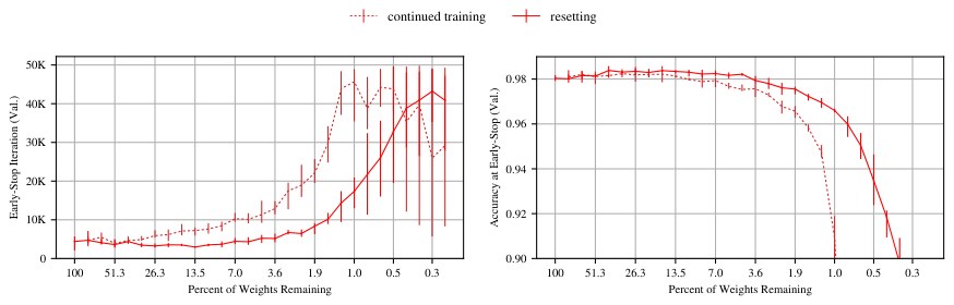
Figure 9: The early-stopping iteration and accuracy at early-stopping of the iterative lottery ticket experiment on the Lenet architecture when iteratively pruned using the resetting and continued training strategies.

图 9：在 Lenet 结构上，分别用重置策略和继续训练策略做迭代剪枝时，迭代彩票实验的早停迭代以及早停时的精度。

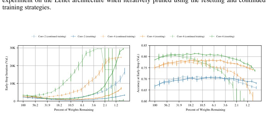
Figure 10: The early-stopping iteration and accuracy at early-stopping of the iterative lottery ticket experiment on the Conv-2, Conv-4, and Conv-6 architectures when iteratively pruned using the resetting and continued training strategies.

图 10：在 Conv-2、Conv-4 和 Conv-6 结构上，分别用重置策略和继续训练策略做迭代剪枝时，迭代彩票实验的早停迭代以及早停时的精度。

Figures 9 and 10 compare the two strategies on the Lenet and Conv-2/4/6 architectures on the hyperparameters we select in Appendices G and H. In all cases, the Strategy 1 maintains higher validation accuracy and faster early-stopping times to smaller network sizes.

图 9 和图 10 在附录 G 和 H 中所选的超参数上，比较了两种策略在 Lenet 和 Conv-2/4/6 结构上的表现。在所有情形中，策略 1 都能在更小的网络规模上保持更高的验证精度和更快的早停时间。

Appendix C Early Stopping Criterion

附录 C 早停准则

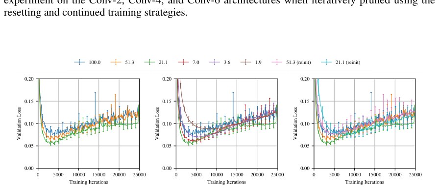
Figure 11: The validation loss data corresponding to Figure 3, i.e., the validation loss as training progresses for several different levels of pruning in the iterative pruning experiment. Each line is the average of five training runs at the same level of iterative pruning; the labels are the percentage of weights from the original network that remain after pruning. Each network was trained with Adam at a learning rate of 0.0012. The left graph shows winning tickets that learn increasingly faster than the original network and reach lower loss. The middle graph shows winning tickets that learn increasingly slower after the fastest early-stopping time has been reached. The right graph contrasts the loss of winning tickets to the loss of randomly reinitialized networks.

图 11：与图 3 对应的验证损失数据，也就是迭代剪枝实验中若干不同剪枝水平上、训练过程中的验证损失。每条线是同一迭代剪枝水平上五次训练运行的平均；标签是剪枝后保留的原网络权重百分比。每个网络都用学习率为 0.0012 的 Adam 训练。左图显示中奖彩票比原网络学得越来越快，并达到更低的损失。中图显示，在达到最快早停时间之后，中奖彩票学得越来越慢。右图把中奖彩票的损失与随机重新初始化网络的损失相对照。

Throughout this paper, we are interested in measuring the speed at which networks learn. As a proxy for this quantity, we measure the iteration at which an early-stopping criterion would end training. The specific criterion we employ is the iteration of minimum validation loss. In this Subsection, we further explain that criterion.

在本文通篇，我们关心的是度量网络学习的速度。作为这一量的代理，我们测量早停准则会结束训练的那一次迭代。我们采用的具体准则是验证损失最低的那一次迭代。在本小节中，我们进一步解释这一准则。

Validation and test loss follow a pattern where they decrease early in the training process, reach a minimum, and then begin to increase as the model overfits to the training data. Figure 11 shows an example of the validation loss as training progresses; these graphs use Lenet, iterative pruning, and Adam with a learning rate of 0.0012 (the learning rate we will select in the following subsection). This Figure shows the validation loss corresponding to the test accuracies in Figure 3.

验证损失和测试损失遵循这样一种模式：它们在训练过程早期下降，达到一个最低点，然后随着模型对训练数据过拟合而开始上升。图 11 给出了训练过程中验证损失的一个例子；这些图使用 Lenet、迭代剪枝，以及学习率为 0.0012 的 Adam（我们将在下一小节选择的学习率）。该图展示的是与图 3 中测试精度相对应的验证损失。

In all cases, validation loss initially drops, after which it forms a clear bottom and then begins increasing again. Our early-stopping criterion identifies this bottom. We consider networks that reach this moment sooner to have learned “faster.” In support of this notion, the ordering in which each experiment meets our early-stopping criterion in Figure 3 is the same order in which each experiment reaches a particular test accuracy threshold in Figure 3.

在所有情形中，验证损失起初下降，随后形成一个清晰的底部，然后再次开始上升。我们的早停准则识别的就是这个底部。我们认为更早到达这一时刻的网络学得“更快”。支持这一看法的是：各实验在图 3 中达到我们早停准则的先后顺序，与各实验在图 3 中达到某一测试精度阈值的顺序相同。

Throughout this paper, in order to contextualize this learning speed, we also present the test accuracy of the network at the iteration of minimum validation loss. In the main body of the paper, we find that winning tickets both arrive at early-stopping sooner and reach higher test accuracy at this point.

在本文通篇，为了给这一学习速度提供语境，我们还给出网络在验证损失最低那一次迭代上的测试精度。在论文正文中，我们发现中奖彩票既更早到达早停，又在这一点上达到更高的测试精度。

Appendix D Training Accuracy for Lottery Ticket Experiments

附录 D 彩票实验中的训练精度

This Appendix accompanies Figure 4 (the accuracy and early-stopping iterations of Lenet on MNIST from Section 2) and Figure 5 (the accuracy and early-stopping iterations of Conv-2, Conv-4, and Conv-6 in Section Section 3) in the main body of the paper. Those figures show the iteration of early-stopping, the test accuracy at early-stopping, the training accuracy at early-stopping, and the test accuracy at the end of the training process. However, we did not have space to include a graph of the training accuracy at the end of the training process, which we assert in the main body of the paper to be 100% for all but the most heavily pruned networks. In this Appendix, we include those additional graphs in Figure 12 (corresponding to Figure 4) and Figure 13 (corresponding to Figure 5). As we describe in the main body of the paper, training accuracy reaches 100% in all cases for all but the most heavily pruned networks. However, training accuracy remains at 100% longer for winning tickets than for randomly reinitialized networks.

本附录配合正文中的图 4（第 2 节 Lenet 在 MNIST 上的精度与早停迭代）和图 5（第 3 节 Conv-2、Conv-4 和 Conv-6 的精度与早停迭代）。那些图展示了早停迭代、早停时的测试精度、早停时的训练精度，以及训练过程结束时的测试精度。不过我们没有空间再放一张训练过程结束时的训练精度图，而我们在正文中断言：除了被剪得最狠的网络之外，这一精度对所有网络都是 100%。在本附录中，我们把这些额外的图放在图 12（对应图 4）和图 13（对应图 5）里。正如我们在正文中所描述的，除了被剪得最狠的网络之外，训练精度在所有情形下都达到 100%。不过，中奖彩票的训练精度保持在 100% 的时间比随机重新初始化的网络更长。

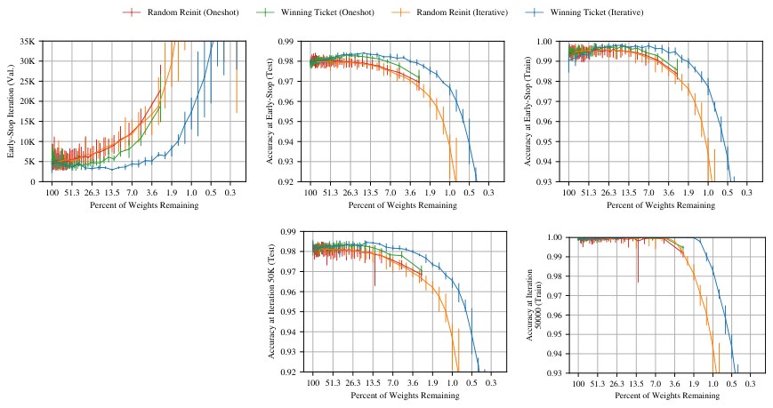
Figure 12: Figure 4 augmented with a graph of the training accuracy at the end of 50,000 iterations.

图 12：在图 4 的基础上增加一张 50,000 次迭代结束时的训练精度图。

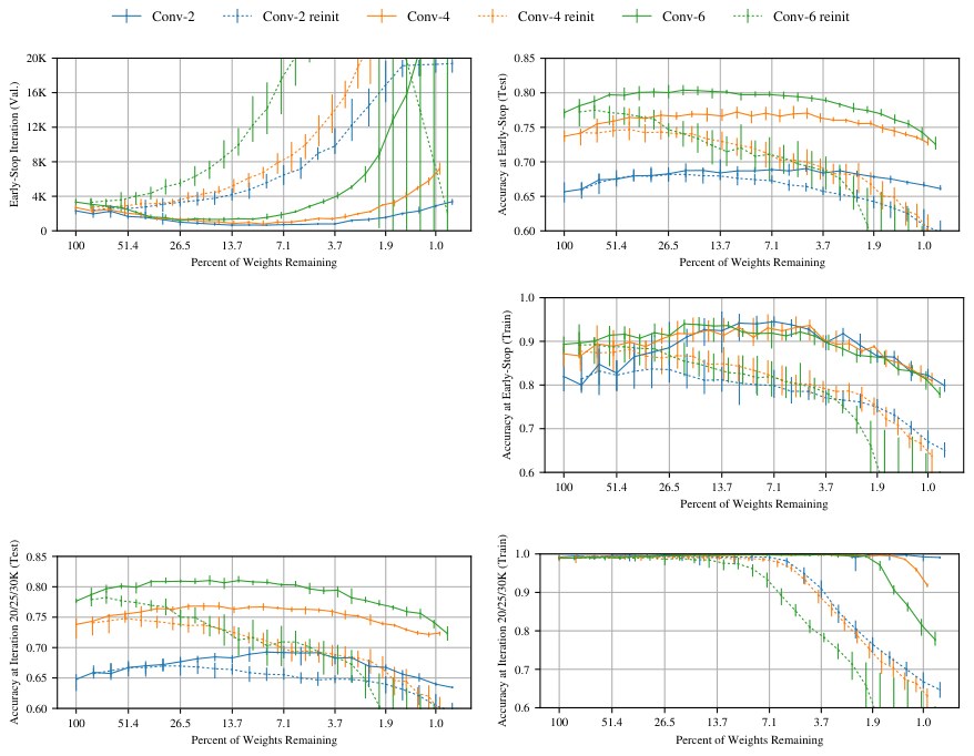
Figure 13: Figure 5 augmented with a graph of the training accuracy at the end of the training process.

图 13：在图 5 的基础上增加一张训练过程结束时的训练精度图。

Appendix E Comparing Random Reinitialization and Random Sparsity

附录 E 比较随机重新初始化与随机稀疏

In this Appendix, we aim to understand the relative performance of randomly reinitialized winning tickets and randomly sparse networks.

在本附录中，我们想理解随机重新初始化的中奖彩票与随机稀疏网络的相对表现。

1. Networks found via iterative pruning with the original initializations (blue in Figure 14).

1. 通过迭代剪枝找到、并保留原来初始化的网络（图 14 中为蓝色）。

2. Networks found via iterative pruning that are randomly reinitialized (orange in Figure 14).

2. 通过迭代剪枝找到、并被随机重新初始化的网络（图 14 中为橙色）。

3. Random sparse subnetworks with the same number of parameters as those found via iterative pruning (green in Figure 14).

3. 与通过迭代剪枝找到的网络具有相同参数量的随机稀疏子网络（图 14 中为绿色）。

Figure 14 shows this comparison for all of the major experiments in this paper. For the fully-connected Lenet architecture for MNIST, we find that the randomly reinitialized networks outperform random sparsity. However, for all of the other, convolutional networks studied in this paper, there is no significant difference in performance between the two. We hypothesize that the fully-connected network for MNIST sees these benefits because only certain parts of the MNIST images contain useful information for classification, meaning connections in some parts of the network will be more valuable than others. This is less true with convolutions, which are not constrained to any one part of the input image.

图 14 对本文所有主要实验展示了这一比较。对于用于 MNIST 的全连接 Lenet 结构，我们发现随机重新初始化的网络优于随机稀疏。不过，对本文研究的所有其他卷积网络，二者的表现没有显著差异。我们猜想，用于 MNIST 的全连接网络之所以看到这些好处，是因为只有 MNIST 图像的某些部分包含对分类有用的信息，意味着网络某些部分的连接会比其他部分更有价值。对卷积来说这一点不那么成立，因为卷积并不被约束在输入图像的某一部分。

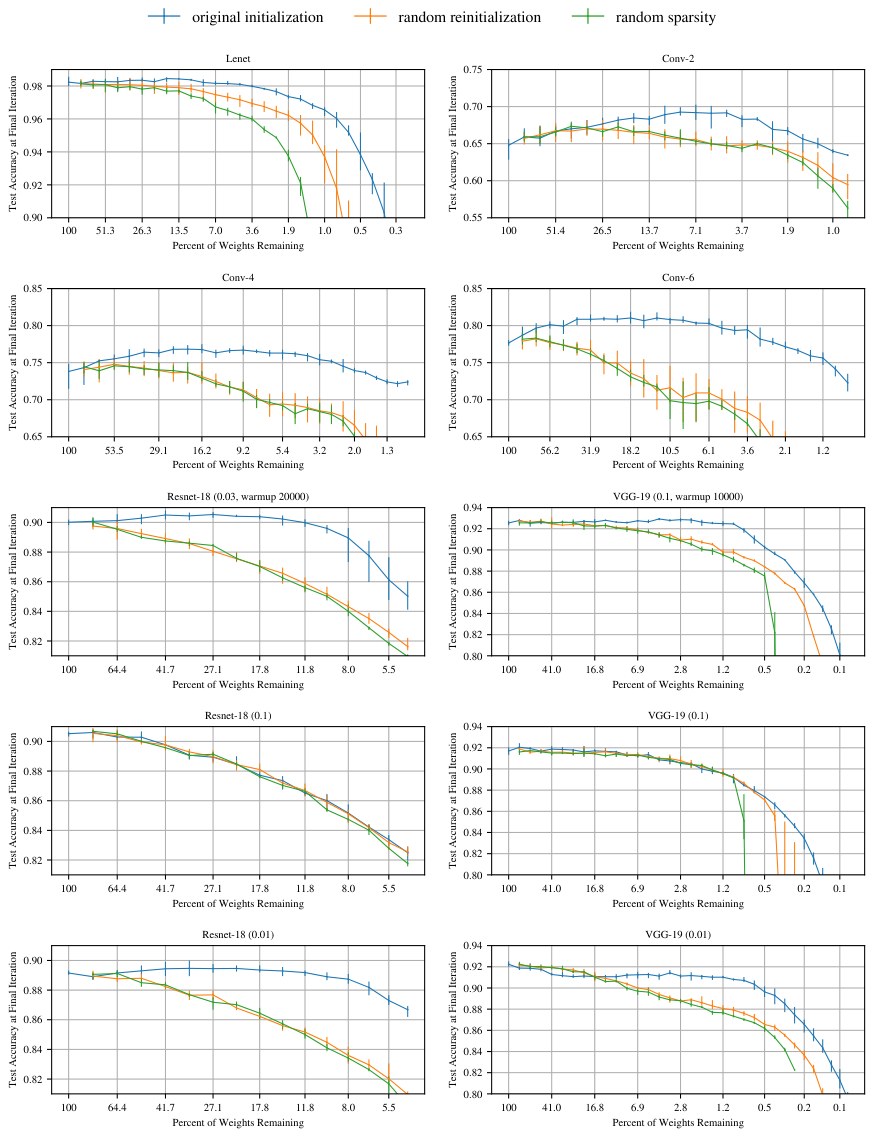
Figure 14: The test accuracy at the final iteration for each of the networks studied in this paper.

图 14：本文所研究的每个网络在最后一次迭代上的测试精度。

Appendix F Examining Winning Tickets

附录 F 审视中奖彩票

In this Appendix, we examine the structure of winning tickets to gain insight into why winning tickets are able to learn effectively even when so heavily pruned. Throughout this Appendix, we study the winning tickets from the Lenet architecture trained on MNIST. Unless otherwise stated, we use the same hyperparameters as in Section 2: glorot initialization and adam optimization.

在本附录中，我们审视中奖彩票的结构，以理解它们为何在被剪得如此厉害时仍能有效学习。本附录通篇研究在 MNIST 上训练的 Lenet 结构的中奖彩票。除非另有说明，我们使用与第 2 节相同的超参数：glorot 初始化和 adam 优化。

F.1 Winning Ticket Initialization (Adam)

F.1 中奖彩票的初始化（Adam）

Figure 15 shows the distributions of winning ticket initializations for four different levels of $P_{m}$. To clarify, these are the distributions of the initial weights of the connections that have survived the pruning process. The blue, orange, and green lines show the distribution of weights for the first hidden layer, second hidden layer, and output layer, respectively. The weights are collected from five different trials of the lottery ticket experiment, but the distributions for each individual trial closely mirror those aggregated from across all of the trials. The histograms have been normalized so that the area under each curve is 1.

图 15 展示了四个不同 $P_{m}$ 水平上中奖彩票初始化的分布。需要说明的是，这些是在剪枝过程中存活下来的连接的初始权重分布。蓝、橙、绿三条线分别表示第一隐层、第二隐层和输出层的权重分布。权重收集自彩票实验的五次不同试验，但每一次试验各自的分布都与把所有试验聚合起来的分布十分接近。直方图已经归一化，使每条曲线下方的面积为 1。

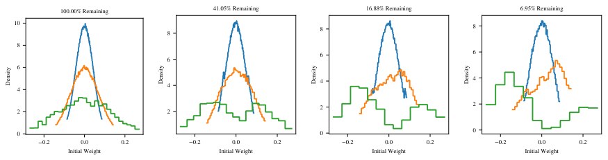
Figure 15: The distribution of initializations in winning tickets pruned to the levels specified in the titles of each plot. The blue, orange, and green lines show the distributions for the first hidden layer, second hidden layer, and output layer of the Lenet architecture for MNIST when trained with the adam optimizer and the hyperparameters used in 2. The distributions have been normalized so that the area under each curve is 1.

图 15：被剪到各分图标题所示水平的中奖彩票中，初始化的分布。蓝、橙、绿三条线分别表示用于 MNIST 的 Lenet 结构在用 adam 优化器以及第 2 节所用超参数训练时，第一隐层、第二隐层和输出层的分布。分布已经归一化，使每条曲线下方的面积为 1。

The left-most graph in Figure 15 shows the initialization distributions for the unpruned networks. We use glorot initialization, so each of the layers has a different standard deviation. As the network is pruned, the first hidden layer maintains its distribution. However, the second hidden layer and the output layer become increasingly bimodal, with peaks on either side of 0. Interestingly, the peaks are asymmetric: the second hidden layer has more positive initializations remaining than negative initializations, and the reverse is true for the output layer.

图 15 最左边的图展示了未剪枝网络的初始化分布。我们使用 glorot 初始化，因此每一层有不同的标准差。随着网络被剪枝，第一隐层保持其分布。然而，第二隐层和输出层变得越来越双峰，峰值分别落在 0 的两侧。有意思的是，这些峰值是不对称的：第二隐层留下的正初始化多于负初始化，输出层则相反。

The connections in the second hidden layer and output layer that survive the pruning process tend to have higher magnitude-initializations. Since we find winning tickets by pruning the connections with the lowest magnitudes in each layer at the end, the connections with the lowest-magnitude initializations must still have the lowest-magnitude weights at the end of training. A different trend holds for the input layer: it maintains its distribution, meaning a connection’s initialization has less relation to its final weight.

在剪枝过程中存活下来的第二隐层和输出层连接，往往具有更大的幅度初始化。由于我们是通过在训练结束时剪掉每一层中幅度最低的连接来寻找中奖彩票的，那些初始化幅度最低的连接在训练结束时必定仍然具有幅度最低的权重。输入层呈现出不同的趋势：它保持其分布，意味着一条连接的初始化与其最终权重的关系更弱。

F.2 Winning Ticket Initializations (SGD)

F.2 中奖彩票的初始化（SGD）

We also consider the winning tickets obtained when training the network with SGD learning rate 0.8 (selected as described in Appendix G). The bimodal distributions from Figure 15 are present across all layers (see Figure 16. The connections with the highest-magnitude initializations are more likely to survive the pruning process, meaning winning ticket initializations have a bimodal distribution with peaks on opposite sides of 0. Just as with the adam-optimized winning tickets, these peaks are of different sizes, with the first hidden layer favoring negative initializations and the second hidden layer and output layer favoring positive initializations. Just as with the adam results, we confirm that each individual trial evidences the same asymmetry as the aggregate graphs in Figure 16.

我们也考虑用学习率为 0.8 的 SGD 训练网络时得到的中奖彩票（按附录 G 所述选定）。图 15 中的双峰分布出现在所有层上（见图 16）。初始化幅度最高的连接更可能在剪枝过程中存活，因此中奖彩票的初始化呈双峰分布，峰值分别落在 0 的两侧。正如用 adam 优化的中奖彩票，这些峰值大小不同：第一隐层偏向负初始化，第二隐层和输出层偏向正初始化。与 adam 的结果一样，我们确认每一次试验都呈现出与图 16 中聚合图相同的不对称性。

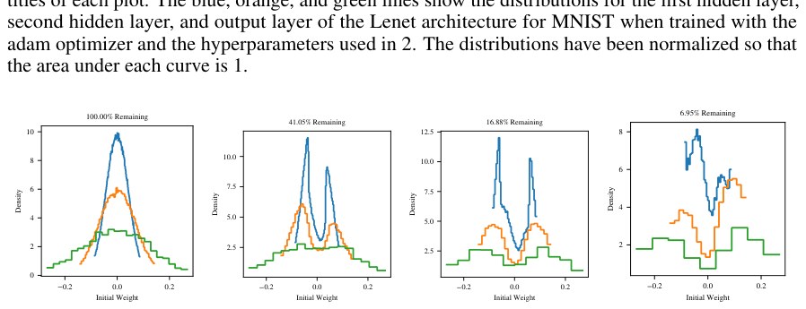
Figure 16: Same as Figure 15 where the network is trained with SGD at rate 0.8.

图 16：与图 15 相同，只是网络用学习率为 0.8 的 SGD 训练。

F.3 Reinitializing from Winning Ticket Initializations

F.3 从中奖彩票的初始化分布重新初始化

Considering that the initialization distributions of winning tickets $\mathcal{D}_{m}$ are so different from the Gaussian distribution $\mathcal{D}$ used to initialize the unpruned network, it is natural to ask whether randomly reinitializing winning tickets from $\mathcal{D}_{m}$ rather than $\mathcal{D}$ will improve winning ticket performance. We do not find this to be the case. Figure 17 shows the performance of winning tickets whose initializations are randomly sampled from the distribution of initializations contained in the winning tickets for adam. More concretely, let $\mathcal{D}_{m}=\{\theta_{0}^{(i)}|m^{(i)}=1\}$ be the set of initializations found in the winning ticket with mask $m$. We sample a new set of parameters $\theta^{\prime}_{0}\sim\mathcal{D}_{m}$ and train the network $f(x;m\odot\theta^{\prime}_{0})$. We perform this sampling on a per-layer basis. The results of this experiment are in Figure 17. Winning tickets reinitialized from $\mathcal{D}_{m}$ perform little better than when randomly reinitialized from $\mathcal{D}$. We attempted the same experiment with the SGD-trained winning tickets and found similar results.

考虑到中奖彩票的初始化分布 $\mathcal{D}_{m}$ 与用于初始化未剪枝网络的高斯分布 $\mathcal{D}$ 如此不同，自然要问：若从 $\mathcal{D}_{m}$ 而不是 $\mathcal{D}$ 中随机重新初始化中奖彩票，是否会改善中奖彩票的表现。我们没有发现情况如此。图 17 展示了其初始化从 adam 中奖彩票所含初始化的分布中随机采样的中奖彩票的表现。更具体地说，令 $\mathcal{D}_{m}=\{\theta_{0}^{(i)}|m^{(i)}=1\}$ 为掩码为 $m$ 的中奖彩票中找到的初始化集合。我们采样一组新参数 $\theta^{\prime}_{0}\sim\mathcal{D}_{m}$，并训练网络 $f(x;m\odot\theta^{\prime}_{0})$。我们按层进行这一采样。该实验的结果见图 17。从 $\mathcal{D}_{m}$ 重新初始化的中奖彩票，表现几乎不比从 $\mathcal{D}$ 随机重新初始化时更好。我们在用 SGD 训练的中奖彩票上做了同样的实验，结果类似。

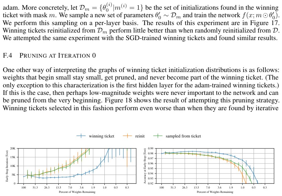
Figure 17: The performance of the winning tickets of the Lenet architecture for MNIST when the layers are randomly reinitialized from the distribution of initializations contained in the winning ticket of the corresponding size.

图 17：用于 MNIST 的 Lenet 结构的中奖彩票，在各层从对应规模中奖彩票所含初始化的分布中被随机重新初始化时的表现。

F.4 Pruning at Iteration 0

F.4 在第 0 次迭代剪枝

One other way of interpreting the graphs of winning ticket initialization distributions is as follows: weights that begin small stay small, get pruned, and never become part of the winning ticket. (The only exception to this characterization is the first hidden layer for the adam-trained winning tickets.) If this is the case, then perhaps low-magnitude weights were never important to the network and can be pruned from the very beginning. Figure 18 shows the result of attempting this pruning strategy. Winning tickets selected in this fashion perform even worse than when they are found by iterative pruning and randomly reinitialized. We attempted the same experiment with the SGD-trained winning tickets and found similar results.

解读中奖彩票初始化分布图的另一种方式如下：一开始就很小的权重一直很小，被剪掉，从未成为中奖彩票的一部分。（对这一刻画的唯一例外，是用 adam 训练的中奖彩票的第一隐层。）如果情况如此，那么低幅度权重也许对网络从未重要，可以从一开始就被剪掉。图 18 展示了尝试这一剪枝策略的结果。以这种方式选出的中奖彩票，表现甚至差于通过迭代剪枝找到后再随机重新初始化。我们在用 SGD 训练的中奖彩票上做了同样的实验，结果类似。

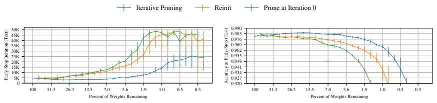
Figure 18: The performance of the winning tickets of the Lenet architecture for MNIST when magnitude pruning is performed before the network is ever trained. The network is subsequently trained with adam.

图 18：用于 MNIST 的 Lenet 结构的中奖彩票，在网络尚未训练时就进行幅度剪枝时的表现。网络随后用 adam 训练。

F.5 Comparing Initial and Final Weights in Winning Tickets

F.5 比较中奖彩票中的初始与最终权重

In this subsection, we consider winning tickets in the context of the larger optimization process. To do so, we examine the initial and final weights of the unpruned network from which a winning ticket derives to determine whether weights that will eventually comprise a winning ticket exhibit properties that distinguish them from the rest of the network.

在本小节中，我们在更大的优化过程语境下考虑中奖彩票。为此，我们考察中奖彩票所源自的未剪枝网络的初始与最终权重，以确定那些最终会构成中奖彩票的权重是否呈现出使它们有别于网络其余部分的性质。

We consider the magnitude of the difference between initial and final weights. One possible rationale for the success of winning tickets is that they already happen to be close to the optimum that gradient descent eventually finds, meaning that winning ticket weights should change by a smaller amount than the rest of the network. Another possible rationale is that winning tickets are well placed in the optimization landscape for gradient descent to optimize productively, meaning that winning ticket weights should change by a larger amount than the rest of the network. Figure 19 shows that winning ticket weights tend to change by a larger amount then weights in the rest of the network, evidence that does not support the rationale that winning tickets are already close to the optimum.

我们考虑初始权重与最终权重之差的幅度。对中奖彩票为何成功的一种可能理由是：它们碰巧已经接近梯度下降最终找到的最优点，这意味着中奖彩票的权重应当比网络其余部分变化更小。另一种可能理由是：中奖彩票在优化地形中处于便于梯度下降有效优化的位置，这意味着中奖彩票的权重应当比网络其余部分变化更大。图 19 表明，中奖彩票的权重往往比网络其余部分的权重变化更大，这一证据并不支持“中奖彩票已经接近最优点”的理由。

It is notable that such a distinction exists between the two distributions. One possible explanation for this distinction is that the notion of a winning ticket may indeed be a natural part of neural network optimization. Another is that magnitude-pruning biases the winning tickets we find toward those containing weights that change in the direction of higher magnitude. Regardless, it offers hope that winning tickets may be discernible earlier in the training process (or after a single training run), meaning that there may be more efficient methods for finding winning tickets than iterative pruning.

这两种分布之间存在这样的区分，这一点值得留意。对这一区分的一种可能解释是：中奖彩票这一概念或许确实是神经网络优化中自然的一部分。另一种解释是：基于幅度的剪枝使我们找到的中奖彩票偏向于包含那些朝更大幅度方向变化的权重。无论如何，它带来一个希望：中奖彩票或许能在训练过程更早的时候（或在单次训练运行之后）被辨别出来，这意味着可能存在比迭代剪枝更高效的寻找中奖彩票的方法。

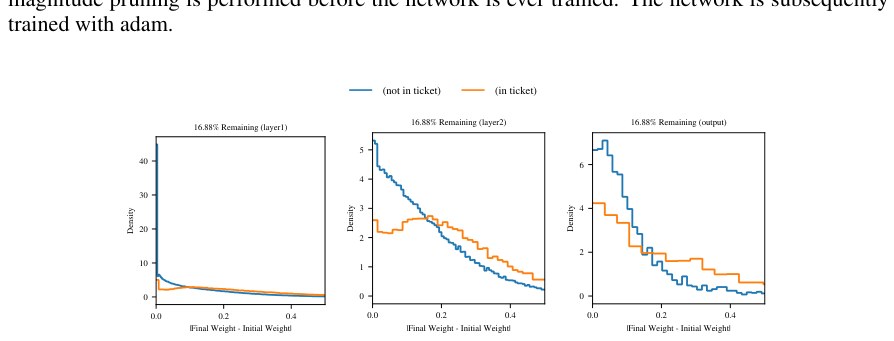
Figure 19: Between the first and last training iteration of the unpruned network, the magnitude by which weights in the network change. The blue line shows the distribution of magnitudes for weights that are not in the eventual winning ticket; the orange line shows the distribution of magnitudes for weights that are in the eventual winning ticket.

图 19：在未剪枝网络的第一次与最后一次训练迭代之间，网络中权重变化的幅度。蓝线展示最终不在中奖彩票中的权重的幅度分布；橙线展示最终在中奖彩票中的权重的幅度分布。

Figure 20 shows the directions of these changes. It plots the difference between the magnitude of the final weight and the magnitude of the initial weight, i.e., whether the weight moved toward or away from 0. In general, winning ticket weights are more likely to increase in magnitude (that is, move away from 0) than are weights that do not participate in the eventual winning ticket.

图 20 展示这些变化的方向。它画出最终权重幅度与初始权重幅度之差，也就是权重是朝向还是远离 0 移动。总体而言，中奖彩票的权重比那些不参与最终中奖彩票的权重更可能增大幅度（也就是远离 0）。

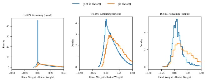
Figure 20: Between the first and last training iteration of the unpruned network, the magnitude by which weights move away from 0. The blue line shows the distribution of magnitudes for weights that are not in the eventual winning ticket; the orange line shows the distribution of magnitudes for weights that are in the eventual winning ticket.

图 20：在未剪枝网络的第一次与最后一次训练迭代之间，权重大幅度远离 0 的幅度。蓝线展示最终不在中奖彩票中的权重的幅度分布；橙线展示最终在中奖彩票中的权重的幅度分布。

F.6 Winning Ticket Connectivity

F.6 中奖彩票的连通性

In this Subsection, we study the connectivity of winning tickets. Do some hidden units retain a large number of incoming connections while others fade away, or does the network retain relatively even sparsity among all units as it is pruned? We find the latter to be the case when examining the incoming connectivity of network units: for both adam and SGD, each unit retains a number of incoming connections approximately in proportion to the amount by which the overall layer has been pruned. Figures 21 and 22 show the fraction of incoming connections that survive the pruning process for each node in each layer. Recall that we prune the output layer at half the rate as the rest of the network, which explains why it has more connectivity than the other layers of the network.

在本小节中，我们研究中奖彩票的连通性。是一些隐单元保留了大量传入连接而另一些逐渐消失，还是网络在被剪枝时在所有单元之间保持相对均匀的稀疏性？在考察网络单元的传入连通性时，我们发现情况是后者：无论是 adam 还是 SGD，每个单元保留的传入连接数大致与该层整体被剪掉的比例成正比。图 21 和图 22 展示每一层中每个节点在剪枝过程中存活下来的传入连接比例。请记住，我们以网络其余部分一半的比率对输出层剪枝，这解释了为何它比网络其他层有更多连通性。

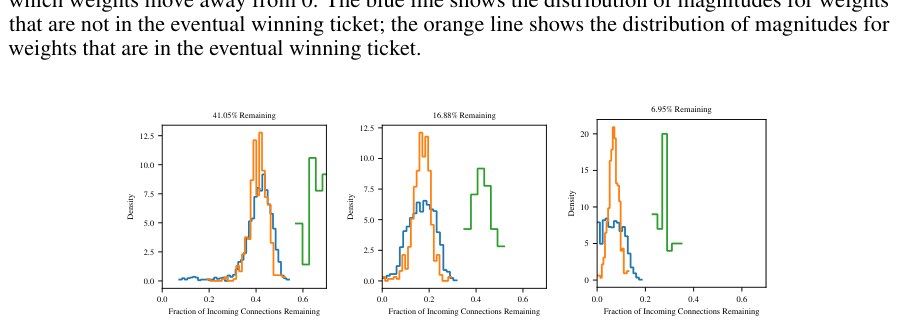
Figure 21: The fraction of incoming connections that survive the pruning process for each node in each layer of the Lenet architecture for MNIST as trained with adam.

图 21：用于 MNIST 的 Lenet 结构在用 adam 训练时，每一层中每个节点在剪枝过程中存活下来的传入连接比例。

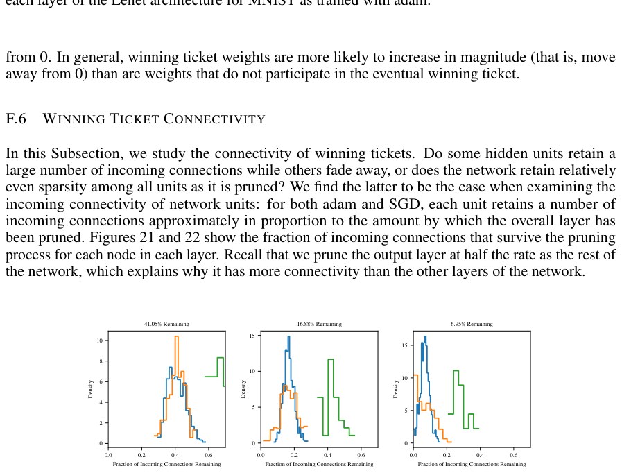
Figure 22: Same as Figure 21 where the network is trained with SGD at rate 0.8.

图 22：与图 21 相同，只是网络用学习率为 0.8 的 SGD 训练。

However, this is not the case for the outgoing connections. To the contrary, for the adam-trained networks, certain units retain far more outgoing connections than others (Figure 23). The distributions are far less smooth than those for the incoming connections, suggesting that certain features are far more useful to the network than others. This is not unexpected for a fully-connected network on a task like MNIST, particularly for the input layer: MNIST images contain centered digits, so the pixels around the edges are not likely to be informative for the network. Indeed, the input layer has two peaks, one larger peak for input units with a high number of outgoing connections and one smaller peak for input units with a low number of outgoing connections. Interestingly, the adam-trained winning tickets develop a much more uneven distribution of outgoing connectivity for the input layer than does the SGD-trained network (Figure 24).

不过，传出连接的情况并非如此。相反，对用 adam 训练的网络，某些单元保留的传出连接远多于其他单元（图 23）。这些分布远不如传入连接的分布平滑，表明某些特征对网络远比其他特征有用。对 MNIST 这类任务上的全连接网络来说，这一点并不意外，尤其是对输入层：MNIST 图像包含居中的数字，因此边缘附近的像素不太可能对网络有信息量。事实上，输入层有两个峰值，一个较大的峰值对应有大量传出连接的输入单元，一个较小的峰值对应传出连接很少的输入单元。有意思的是，用 adam 训练的中奖彩票在输入层发展出的传出连通性分布，比用 SGD 训练的网络（图 24）不均匀得多。

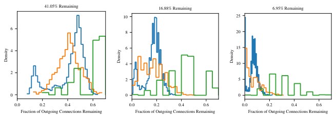
Figure 23: The fraction of outgoing connections that survive the pruning process for each node in each layer of the Lenet architecture for MNIST as trained with adam. The blue, orange, and green lines are the outgoing connections from the input layer, first hidden layer, and second hidden layer, respectively.

图 23：用于 MNIST 的 Lenet 结构在用 adam 训练时，每一层中每个节点在剪枝过程中存活下来的传出连接比例。蓝、橙、绿三条线分别是来自输入层、第一隐层和第二隐层的传出连接。

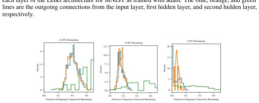
Figure 24: Same as Figure 23 where the network is trained with SGD at rate 0.8.

图 24：与图 23 相同，只是网络用学习率为 0.8 的 SGD 训练。

F.7 Adding Noise to Winning Tickets

F.7 向中奖彩票添加噪声

In this Subsection, we explore the extent to which winning tickets are robust to Gaussian noise added to their initializations. In the main body of the paper, we find that randomly reinitializing a winning ticket substantially slows its learning and reduces its eventual test accuracy. In this Subsection, we study a less extreme way of perturbing a winning ticket. Figure 25 shows the effect of adding Gaussian noise to the winning ticket initializations. The standard deviation of the noise distribution of each layer is a multiple of the standard deviation of the layer’s initialization Figure 25 shows noise distributions with standard deviation $0.5\sigma$, $\sigma$, $2\sigma$, and $3\sigma$. Adding Gaussian noise reduces the test accuracy of a winning ticket and slows its ability to learn, again demonstrating the importance of the original initialization. As more noise is added, accuracy decreases. However, winning tickets are surprisingly robust to noise. Adding noise of $0.5\sigma$ barely changes winning ticket accuracy. Even after adding noise of $3\sigma$, the winning tickets continue to outperform the random reinitialization experiment.

在本小节中，我们探索中奖彩票对其初始化上所加高斯噪声的稳健程度。在论文正文中，我们发现随机重新初始化一张中奖彩票会显著减慢其学习并降低其最终测试精度。在本小节中，我们研究一种不那么极端的扰动中奖彩票的方式。图 25 展示向中奖彩票的初始化添加高斯噪声的效果。每一层噪声分布的标准差是该层初始化标准差的一个倍数。图 25 展示标准差为 $0.5\sigma$、$\sigma$、$2\sigma$ 和 $3\sigma$ 的噪声分布。添加高斯噪声会降低中奖彩票的测试精度并减慢其学习能力，再次说明原来的初始化很重要。添加的噪声越多，精度下降越多。不过，中奖彩票对噪声出人意料地稳健。添加 $0.5\sigma$ 的噪声几乎不改变中奖彩票的精度。即便添加 $3\sigma$ 的噪声之后，中奖彩票仍然继续优于随机重新初始化实验。

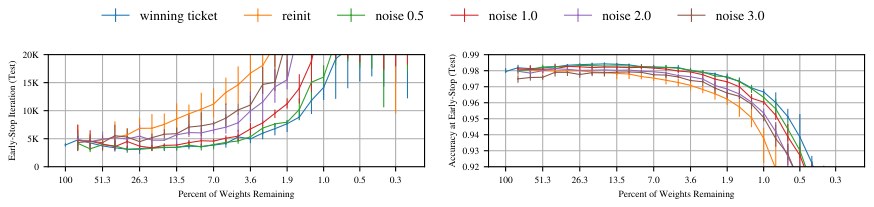
Figure 25: The performance of the winning tickets of the Lenet architecture for MNIST when Gaussian noise is added to the initializations. The standard deviations of the noise distributions for each layer are a multiple of the standard deviations of the initialization distributions; in this Figure, we consider multiples 0.5, 1, 2, and 3.

图 25：用于 MNIST 的 Lenet 结构的中奖彩票在初始化上添加高斯噪声时的表现。每一层噪声分布的标准差是初始化分布标准差的一个倍数；在本图中，我们考虑倍数 0.5、1、2 和 3。

Appendix G Hyperparameter Exploration for Fully-Connected Networks

附录 G 全连接网络的超参数探索

This Appendix accompanies Section 2 of the main paper. It explores the space of hyperparameters for the Lenet architecture evaluated in Section 2 with two purposes in mind:

本附录配合正文第 2 节。它探索第 2 节所评估的 Lenet 结构的超参数空间，目的有二：

1. To explain the hyperparameters selected in the main body of the paper.

1. 解释正文中所选的超参数。

2. To evaluate the extent to which the lottery ticket experiment patterns extend to other choices of hyperparameters.

2. 评估彩票实验的模式在多大程度上延伸到其他超参数选择。

G.1 Experimental Methodology

G.1 实验方法

This Section considers the fully-connected Lenet architecture (LeCun et al., 1998), which comprises two fully-connected hidden layers and a ten unit output layer, on the MNIST dataset. Unless otherwise stated, the hidden layers have 300 and 100 units each.

本节考虑全连接 Lenet 结构（LeCun et al., 1998）在 MNIST 数据集上的表现，该结构包含两个全连接隐层和一个十单元输出层。除非另有说明，隐层分别有 300 和 100 个单元。

The MNIST dataset consists of 60,000 training examples and 10,000 test examples. We randomly sampled a 5,000-example validation set from the training set and used the remaining 55,000 training examples as our training set for the rest of the paper (including Section 2). The hyperparameter selection experiments throughout this Appendix are evaluated using the validation set for determining both the iteration of early-stopping and the accuracy at early-stopping; the networks in the main body of this paper (which make use of these hyperparameters) have their accuracy evaluated on the test set. The training set is presented to the network in mini-batches of 60 examples; at each epoch, the entire training set is shuffled.

MNIST 数据集由 60,000 个训练样本和 10,000 个测试样本组成。我们从训练集中随机采样了一个 5,000 样本的验证集，并把剩下的 55,000 个训练样本作为本文其余部分（包括第 2 节）的训练集。本附录中的超参数选择实验用验证集来确定早停迭代以及早停时的精度；正文中的网络（使用这些超参数）在测试集上评估精度。训练集以每批 60 个样本的小批量呈现给网络；在每个周期，整个训练集都会被打乱。

Unless otherwise noted, each line in each graph comprises data from three separate experiments. The line itself traces the average performance of the experiments and the error bars indicate the minimum and maximum performance of any one experiment.

除非另有说明，每张图中的每条线都包含来自三次独立实验的数据。线本身描画这些实验的平均表现，误差条标出任何一次实验的最小与最大表现。

Throughout this Appendix, we perform the lottery ticket experiment iteratively with a pruning rate of 20% per iteration (10% for the output layer); we justify the choice of this pruning rate later in this Appendix. Each layer of the network is pruned independently. On each iteration of the lottery ticket experiment, the network is trained for 50,000 training iterations regardless of when early-stopping occurs; in other words, no validation or test data is taken into account during the training process, and early-stopping times are determined retroactively by examining validation performance. We evaluate validation and test performance every 100 iterations.

在本附录通篇，我们以每轮 20% 的剪枝率（输出层为 10%）迭代地进行彩票实验；我们稍后在本附录中为这一剪枝率给出理由。网络的每一层被独立剪枝。在彩票实验的每一轮中，无论早停何时发生，网络都被训练 50,000 次训练迭代；换句话说，训练过程中不考虑验证或测试数据，早停时间是事后通过考察验证表现确定的。我们每 100 次迭代评估一次验证和测试表现。

For the main body of the paper, we opt to use the Adam optimizer (Kingma & Ba, 2014) and Gaussian Glorot initialization (Glorot & Bengio, 2010). Although we can achieve more impressive results on the lottery ticket experiment with other hyperparameters, we intend these choices to be as generic as possible in an effort to minimize the extent to which our main results depend on hand-chosen hyperparameters. In this Appendix, we select the learning rate for Adam that we use in the main body of the paper.

对论文正文，我们选择使用 Adam 优化器（Kingma & Ba, 2014）和高斯 Glorot 初始化（Glorot & Bengio, 2010）。尽管用其他超参数可以在彩票实验上取得更出色的结果，我们希望这些选择尽可能通用，以尽量减少主要结果对手工选定超参数的依赖。在本附录中，我们为正文所用的 Adam 选择学习率。

In addition, we consider a wide range of other hyperparameters, including other optimization algorithms (SGD with and without momentum), initialization strategies (Gaussian distributions with various standard deviations), network sizes (larger and smaller hidden layers), and pruning strategies (faster and slower pruning rates). In each experiment, we vary the chosen hyperparameter while keeping all others at their default values (Adam with the chosen learning rate, Gaussian Glorot initialization, hidden layers with 300 and 100 units). The data presented in this appendix was collected by training variations of the Lenet architecture more than 3,000 times.

此外，我们考虑范围广泛的其他超参数，包括其他优化算法（带或不带动量的 SGD）、初始化策略（具有各种标准差的高斯分布）、网络规模（更大和更小的隐层）以及剪枝策略（更快和更慢的剪枝率）。在每个实验中，我们改变所选超参数，同时把所有其他超参数保持在默认值（具有所选学习率的 Adam、高斯 Glorot 初始化、分别有 300 和 100 个单元的隐层）。本附录中给出的数据，是通过把 Lenet 结构的各种变体训练 3,000 次以上收集到的。

G.2 Learning Rate

G.2 学习率

In this Subsection, we perform the lottery ticket experiment on the Lenet architecture as optimized with Adam, SGD, and SGD with momentum at various learning rates.

在本小节中，我们在用 Adam、SGD 以及带动量的 SGD、并以各种学习率优化的 Lenet 结构上做彩票实验。

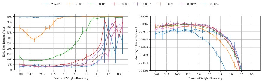
Figure 26: The early-stopping iteration and validation accuracy at that iteration of the iterative lottery ticket experiment on the Lenet architecture trained with MNIST using the Adam optimizer at various learning rates. Each line represents a different learning rate.

图 26：在用各种学习率的 Adam 优化器、于 MNIST 上训练的 Lenet 结构上，迭代彩票实验的早停迭代以及该迭代上的验证精度。每条线代表一种不同的学习率。

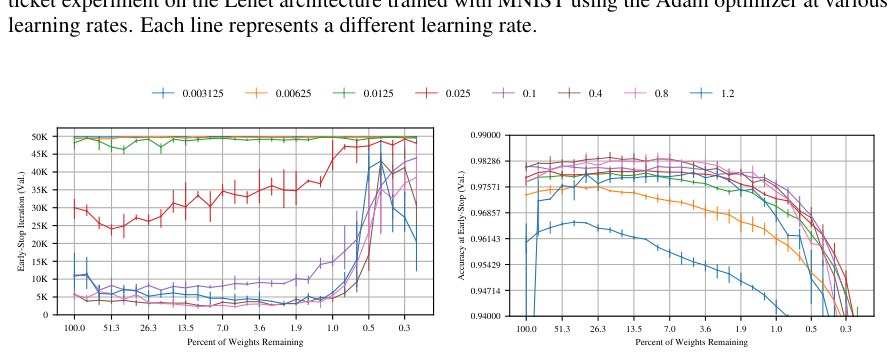
Figure 27: The early-stopping iteration and validation accuracy at that iteration of the iterative lottery ticket experiment on the Lenet architecture trained with MNIST using stochastic gradient descent at various learning rates.

图 27：在用各种学习率的随机梯度下降、于 MNIST 上训练的 Lenet 结构上，迭代彩票实验的早停迭代以及该迭代上的验证精度。

Here, we select the learning rate that we use for Adam in the main body of the paper. Our criteria for selecting the learning rate are as follows:

这里，我们选择正文中为 Adam 使用的学习率。我们选择学习率的准则如下：

1. On the unpruned network, it should minimize training iterations necessary to reach early-stopping and maximize validation accuracy at that iteration. That is, it should be a reasonable hyperparameter for optimizing the unpruned network even if we are not running the lottery ticket experiment.

1. 在未剪枝网络上，它应当最小化达到早停所需的训练迭代，并最大化该迭代上的验证精度。也就是说，即便我们不做彩票实验，它也应当是优化未剪枝网络的合理超参数。

2. When running the iterative lottery ticket experiment, it should make it possible to match the early-stopping iteration and accuracy of the original network with as few parameters as possible.

2. 在运行迭代彩票实验时，它应当使得能够以尽可能少的参数匹配原网络的早停迭代和精度。

3. Of those options that meet (1) and (2), it should be on the conservative (slow) side so that it is more likely to productively optimize heavily pruned networks under a variety of conditions with a variety of hyperparameters.

3. 在满足 (1) 和 (2) 的那些选项中，它应当偏保守（偏慢），以便更可能在各种条件和各种超参数下有效地优化被重度剪枝的网络。

Figure 26 shows the early-stopping iteration and validation accuracy at that iteration of performing the iterative lottery ticket experiment with the Lenet architecture optimized with Adam at various learning rates. According to the graph on the right of Figure 26, several learning rates between 0.0002 and 0.002 achieve similar levels of validation accuracy on the original network and maintain that performance to similar levels as the network is pruned. Of those learning rates, 0.0012 and 0.002 produce the fastest early-stopping times and maintain them to the smallest network sizes. We choose 0.0012 due to its higher validation accuracy on the unpruned network and in consideration of criterion (3) above.

图 26 展示用各种学习率的 Adam 优化 Lenet 结构、进行迭代彩票实验时的早停迭代以及该迭代上的验证精度。根据图 26 右图，介于 0.0002 和 0.002 之间的若干学习率在原网络上达到相近的验证精度水平，并在网络被剪枝时把这一表现保持到相近的程度。在这些学习率中，0.0012 和 0.002 产生最快的早停时间，并把它们保持到最小的网络规模。我们选择 0.0012，是因为它在未剪枝网络上有更高的验证精度，并考虑到上面的准则 (3)。

We note that, across all of these learning rates, the lottery ticket pattern (in which learning becomes faster and validation accuracy increases with iterative pruning) remains present. Even for those learning rates that did not satisfy the early-stopping criterion within 50,000 iterations (2.5e-05 and 0.0064) still showed accuracy improvements with pruning.

我们注意到，在所有这些学习率上，彩票模式（即学习随迭代剪枝变快、验证精度上升）都仍然存在。即便那些未能在 50,000 次迭代内满足早停准则的学习率（2.5e-05 和 0.0064）也仍然随剪枝显示出精度提升。

G.3 Other Optimization Algorithms

G.3 其他优化算法

G.3.1 SGD

Here, we explore the behavior of the lottery ticket experiment when the network is optimized with stochastic gradient descent (SGD) at various learning rates. The results of doing so appear in Figure 27. The lottery ticket pattern appears across all learning rates, including those that fail to satisfy the early-stopping criterion within 50,000 iterations. SGD learning rates 0.4 and 0.8 reach early-stopping in a similar number of iterations as the best Adam learning rates (0.0012 and 0.002) but maintain this performance when the network has been pruned further (to less than 1% of its original size for SGD vs. about 3.6% of the original size for Adam). Likewise, on pruned networks, these SGD learning rates achieve equivalent accuracy to the best Adam learning rates, and they maintain that high accuracy when the network is pruned as much as the Adam learning rates.

G.3.1 SGD

这里，我们探索网络用各种学习率的随机梯度下降（SGD）优化时彩票实验的行为。结果见图 27。彩票模式出现在所有学习率上，包括那些未能在 50,000 次迭代内满足早停准则的学习率。SGD 学习率 0.4 和 0.8 达到早停所需的迭代次数与最好的 Adam 学习率（0.0012 和 0.002）相近，但在网络被进一步剪枝时仍能保持这一表现（SGD 可到原规模的不到 1%，Adam 约为原规模的 3.6%）。同样，在被剪枝的网络上，这些 SGD 学习率达到与最好 Adam 学习率相当的精度，并在网络被剪到与 Adam 学习率同样多时保持这一高精度。

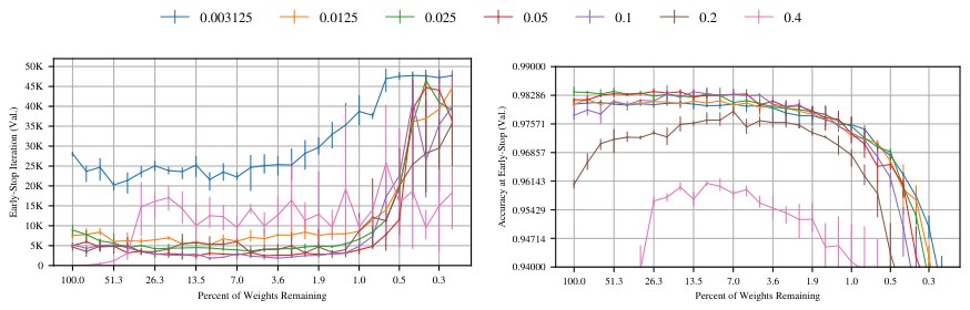
Figure 28: The early-stopping iteration and validation accuracy at that iteration of the iterative lottery ticket experiment on the Lenet architecture trained with MNIST using stochastic gradient descent with momentum (0.9) at various learning rates.

图 28：在用各种学习率的带动量（0.9）随机梯度下降、于 MNIST 上训练的 Lenet 结构上，迭代彩票实验的早停迭代以及该迭代上的验证精度。

G.3.2 Momentum

Here, we explore the behavior of the lottery ticket experiment when the network is optimized with SGD with momentum (0.9) at various learning rates. The results of doing so appear in Figure 28. Once again, the lottery ticket pattern appears across all learning rates, with learning rates between 0.025 and 0.1 maintaining high validation accuracy and faster learning for the longest number of pruning iterations. Learning rate 0.025 achieves the highest validation accuracy on the unpruned network; however, its validation accuracy never increases as it is pruned, instead decreasing gradually, and higher learning rates reach early-stopping faster.

G.3.2 动量

这里，我们探索网络用各种学习率的带动量（0.9）SGD 优化时彩票实验的行为。结果见图 28。彩票模式再次出现在所有学习率上，介于 0.025 和 0.1 之间的学习率在最长的剪枝轮数里保持高验证精度和更快的学习。学习率 0.025 在未剪枝网络上达到最高验证精度；不过，它的验证精度从未随剪枝上升，而是逐渐下降，而更高的学习率更早达到早停。

G.4 Iterative Pruning Rate

G.4 迭代剪枝率

When running the iterative lottery ticket experiment on Lenet, we prune each layer of the network separately at a particular rate. That is, after training the network, we prune $k\%$ of the weights in each layer ($\frac{k}{2}\%$ of the weights in the output layer) before resetting the weights to their original initializations and training again. In the main body of the paper, we find that iterative pruning finds smaller winning tickets than one-shot pruning, indicating that pruning too much of the network at once diminishes performance. Here, we explore different values of $k$.

在 Lenet 上运行迭代彩票实验时，我们以某一比率分别对网络的每一层剪枝。也就是说，在训练网络之后，我们剪掉每一层中 $k\%$ 的权重（输出层中 $\frac{k}{2}\%$ 的权重），再把权重重置为原来的初始化并再次训练。在论文正文中，我们发现迭代剪枝能比一次性剪枝找到更小的中奖彩票，说明一次剪掉网络太多会损害表现。这里，我们探索不同的 $k$ 值。

Figure 29 shows the effect of the amount of the network pruned on each pruning iteration on early-stopping time and validation accuracy. There is a tangible difference in learning speed and validation accuracy at early-stopping between the lowest pruning rates (0.1 and 0.2) and higher pruning rates (0.4 and above). The lowest pruning rates reach higher validation accuracy and maintain that validation accuracy to smaller network sizes; they also maintain fast early-stopping times to smaller network sizes. For the experiments throughout the main body of the paper and this Appendix, we use a pruning rate of 0.2, which maintains much of the accuracy and learning speed of 0.1 while reducing the number of training iterations necessary to get to smaller network sizes.

图 29 展示每一轮剪枝所剪掉的网络量对早停时间和验证精度的影响。最低剪枝率（0.1 和 0.2）与更高剪枝率（0.4 及以上）之间，在学习速度和早停时的验证精度上有切实的差别。最低剪枝率达到更高的验证精度，并把该验证精度保持到更小的网络规模；它们也把很快的早停时间保持到更小的网络规模。对正文和本附录中的实验，我们使用 0.2 的剪枝率，它保持了 0.1 的大部分精度和学习速度，同时减少了到达更小网络规模所需的训练迭代次数。

In all of the Lenet experiments, we prune the output layer at half the rate of the rest of the network. Since the output layer is so small (1,000 weights out of 266,000 for the overall Lenet architecture), we found that pruning it reaches a point of diminishing returns much earlier the other layers.

在所有 Lenet 实验中，我们以网络其余部分一半的比率对输出层剪枝。由于输出层很小（在整个 Lenet 结构的 266,000 个权重中只有 1,000 个），我们发现对它剪枝会比其他层更早到达收益递减的点。

G.5 Initialization Distribution

G.5 初始化分布

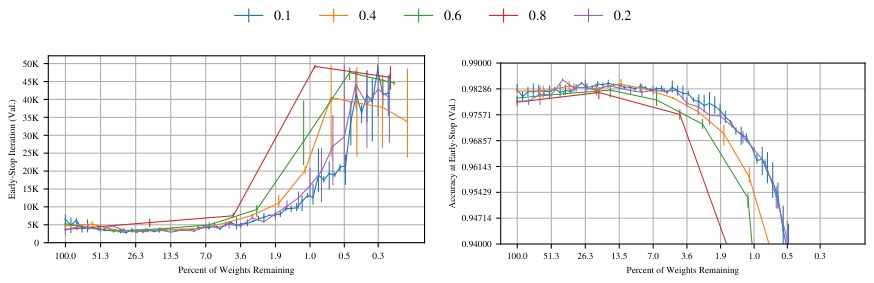
Figure 29: The early-stopping iteration and validation accuracy at that iteration of the iterative lottery ticket experiment when pruned at different rates. Each line represents a different pruning rate—the percentage of lowest-magnitude weights that are pruned from each layer after each training iteration.

图 29：以不同比率剪枝时，迭代彩票实验的早停迭代以及该迭代上的验证精度。每条线代表一种不同的剪枝率——每次训练迭代之后从每一层剪掉的最低幅度权重的百分比。

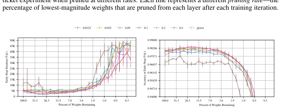
Figure 30: The early-stopping iteration and validation accuracy at that iteration of the iterative lottery ticket experiment initialized with Gaussian distributions with various standard deviations. Each line is a different standard deviation for a Gaussian distribution centered at 0.

图 30：用各种标准差的高斯分布初始化时，迭代彩票实验的早停迭代以及该迭代上的验证精度。每条线是一个中心在 0 的高斯分布的不同标准差。

To this point, we have considered only a Gaussian Glorot (Glorot & Bengio, 2010) initialization scheme for the network. Figure 30 performs the lottery ticket experiment while initializing the Lenet architecture from Gaussian distributions with a variety of standard deviations. The networks were optimized with Adam at the learning rate chosen earlier. The lottery ticket pattern continues to appear across all standard deviations. When initialized from a Gaussian distribution with standard deviation 0.1, the Lenet architecture maintained high validation accuracy and low early-stopping times for the longest, approximately matching the performance of the Glorot-initialized network.

到目前为止，我们只考虑了网络的高斯 Glorot（Glorot & Bengio, 2010）初始化方案。图 30 在用各种标准差的高斯分布初始化 Lenet 结构时进行彩票实验。网络用前面选定学习率的 Adam 优化。彩票模式继续出现在所有标准差上。当从标准差为 0.1 的高斯分布初始化时，Lenet 结构把高验证精度和低早停时间保持得最久，大致匹配 Glorot 初始化网络的表现。

G.6 Network Size

G.6 网络规模

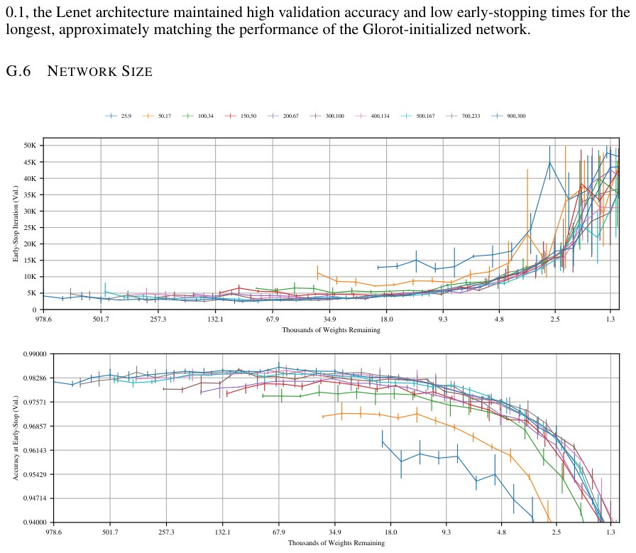
Figure 31: The early-stopping iteration and validation accuracy at at that iteration of the iterative lottery ticket experiment on the Lenet architecture with various layer sizes. The label for each line is the size of the first and second hidden layers of the network. All networks had Gaussian Glorot initialization and were optimized with Adam (learning rate 0.0012). Note that the x-axis of this plot charts the number of weights remaining, while all other graphs in this section have charted the percent of weights remaining.

图 31：在具有各种层规模的 Lenet 结构上，迭代彩票实验的早停迭代以及该迭代上的验证精度。每条线的标签是网络第一和第二隐层的规模。所有网络都使用高斯 Glorot 初始化，并用 Adam（学习率 0.0012）优化。需要注意，本图的 x 轴标出的是剩余权重的数量，而本节中所有其他图标出的都是剩余权重的百分比。

Throughout this section, we have considered the Lenet architecture with 300 units in the first hidden layer and 100 units in the second hidden layer. Figure 31 shows the early-stopping iterations and validation accuracy at that iteration of the Lenet architecture with several other layer sizes. All networks we tested maintain the 3:1 ratio between units in the first hidden layer and units in the second hidden layer.

在本节通篇，我们考虑第一隐层有 300 个单元、第二隐层有 100 个单元的 Lenet 结构。图 31 展示若干其他层规模下 Lenet 结构的早停迭代以及该迭代上的验证精度。我们测试的所有网络都保持第一隐层单元数与第二隐层单元数之间 3:1 的比率。

The lottery ticket hypothesis naturally invites a collection of questions related to network size. Generalizing, those questions tend to take the following form: according to the lottery ticket hypothesis, do larger networks, which contain more subnetworks, find “better” winning tickets? In line with the generality of this question, there are several different answers.

彩票假设自然引出一组与网络规模相关的问题。概括起来，这些问题往往采取如下形式：根据彩票假设，更大的网络包含更多子网络，它们是否会找到“更好”的中奖彩票？与这一问题的一般性相符，答案有好几种。

If we evaluate a winning ticket by the accuracy it achieves, then larger networks do find better winning tickets. The right graph in Figure 31 shows that, for any particular number of weights (that is, any particular point on the x-axis), winning tickets derived from initially larger networks reach higher accuracy. Put another way, in terms of accuracy, the lines are approximately arranged from bottom to top in increasing order of network size. It is possible that, since larger networks have more subnetworks, gradient descent found a better winning ticket. Alternatively, the initially larger networks have more units even when pruned to the same number of weights as smaller networks, meaning they are able to contain sparse subnetwork configurations that cannot be expressed by initially smaller networks.

如果我们用中奖彩票达到的精度来评估它，那么更大的网络确实找到更好的中奖彩票。图 31 右图表明，对任何特定的权重数量（也就是 x 轴上的任何特定点），源自最初更大网络的中奖彩票达到更高精度。换句话说，就精度而言，这些线大致按网络规模递增的顺序从下到上排列。有可能是因为更大的网络有更多子网络，梯度下降找到了更好的中奖彩票。或者，最初更大的网络即使被剪到与更小网络相同的权重数量，也仍有更多单元，因此它们能够包含最初更小的网络无法表达的稀疏子网络配置。

If we evaluate a winning ticket by the time necessary for it to reach early-stopping, then larger networks have less of an advantage. The left graph in Figure 31 shows that, in general, early-stopping iterations do not vary greatly between networks of different initial sizes that have been pruned to the same number of weights. Upon exceedingly close inspection, winning tickets derived from initially larger networks tend to learn marginally faster than winning tickets derived from initially smaller networks, but these differences are slight.

如果我们用达到早停所需的时间来评估中奖彩票，那么更大的网络优势较小。图 31 左图表明，总体而言，被剪到相同权重数量、但最初规模不同的网络之间，早停迭代差异不大。非常仔细地观察会发现，源自最初更大网络的中奖彩票往往比源自最初更小网络的中奖彩票学得略快，但这些差异很小。

If we evaluate a winning ticket by the size at which it returns to the same accuracy as the original network, the large networks do not have an advantage. Regardless of the initial network size, the right graph in Figure 31 shows that winning tickets return to the accuracy of the original network when they are pruned to between about 9,000 and 15,000 weights.

如果我们用中奖彩票回到与原网络相同精度时的规模来评估它，大网络并没有优势。无论最初网络规模如何，图 31 右图表明，中奖彩票在被剪到大约 9,000 到 15,000 个权重时回到原网络的精度。

Appendix H Hyperparameter Exploration for Convolutional Networks

附录 H 卷积网络的超参数探索

This Appendix accompanies Sections 3 of the main paper. It explores the space of optimization algorithms and hyperparameters for the Conv-2, Conv-4, and Conv-6 architectures evaluated in Section 3 with the same two purposes as Appendix G: explaining the hyperparameters used in the main body of the paper and evaluating the lottery ticket experiment on other choices of hyperparameters.

本附录配合正文第 3 节。它探索第 3 节所评估的 Conv-2、Conv-4 和 Conv-6 结构的优化算法与超参数空间，目的与附录 G 相同：解释正文所用的超参数，并在其他超参数选择上评估彩票实验。

H.1 Experimental Methodology

H.1 实验方法

The Conv-2, Conv-4, and Conv-6 architectures are variants of the VGG (Simonyan & Zisserman, 2014) network architecture scaled down for the CIFAR10 (Krizhevsky & Hinton, 2009) dataset. Like VGG, the networks consist of a series of modules. Each module has two layers of 3x3 convolutional filters followed by a maxpool layer with stride 2. After all of the modules are two fully-connected layers of size 256 followed by an output layer of size 10; in VGG, the fully-connected layers are of size 4096 and the output layer is of size 1000. Like VGG, the first module has 64 convolutions in each layer, the second has 128, the third has 256, etc. The Conv-2, Conv-4, and Conv-6 architectures have 1, 2, and 3 modules, respectively.

Conv-2、Conv-4 和 Conv-6 结构是为 CIFAR10（Krizhevsky & Hinton, 2009）数据集缩小的 VGG（Simonyan & Zisserman, 2014）网络结构变体。与 VGG 一样，这些网络由一系列模块组成。每个模块有两层 3x3 卷积滤波器，后接一个步幅为 2 的最大池化层。在所有模块之后是两个规模为 256 的全连接层，再接一个规模为 10 的输出层；在 VGG 中，全连接层规模为 4096，输出层规模为 1000。与 VGG 一样，第一个模块每层有 64 个卷积，第二个有 128 个，第三个有 256 个，依此类推。Conv-2、Conv-4 和 Conv-6 结构分别有 1、2 和 3 个模块。

The CIFAR10 dataset consists of 50,000 32x32 color (three-channel) training examples and 10,000 test examples. We randomly sampled a 5,000-example validation set from the training set and used the remaining 45,000 training examples as our training set for the rest of the paper. The hyperparameter selection experiments throughout this Appendix are evaluated on the validation set, and the examples in the main body of this paper (which make use of these hyperparameters) are evaluated on test set. The training set is presented to the network in mini-batches of 60 examples; at each epoch, the entire training set is shuffled.

CIFAR10 数据集由 50,000 个 32x32 彩色（三通道）训练样本和 10,000 个测试样本组成。我们从训练集中随机采样了一个 5,000 样本的验证集，并把剩下的 45,000 个训练样本作为本文其余部分的训练集。本附录中的超参数选择实验在验证集上评估，正文中的例子（使用这些超参数）在测试集上评估。训练集以每批 60 个样本的小批量呈现给网络；在每个周期，整个训练集都会被打乱。

The Conv-2, Conv-4, and Conv-6 networks are initialized with Gaussian Glorot initialization (Glorot & Bengio, 2010) and are trained for the number of iterations specified in Figure 2. The number of training iterations was selected such that heavily-pruned networks could still train in the time provided. On dropout experiments, the number of training iterations is tripled to provide enough time for the dropout-regularized networks to train. We optimize these networks with Adam, and select the learning rate for each network in this Appendix.

Conv-2、Conv-4 和 Conv-6 网络用高斯 Glorot 初始化（Glorot & Bengio, 2010），并按图 2 中指定的迭代次数训练。训练迭代次数的选择，是为了让被重度剪枝的网络仍然能在所给时间内完成训练。在 dropout 实验中，训练迭代次数增至三倍，以便给用 dropout 正则化的网络足够的训练时间。我们用 Adam 优化这些网络，并在本附录中为每个网络选择学习率。

As with the MNIST experiments, validation and test performance is only considered retroactively and has no effect on the progression of the lottery ticket experiments. We measure validation and test loss and accuracy every 100 training iterations.

与 MNIST 实验一样，验证和测试表现只在事后考虑，对彩票实验的进程没有影响。我们每 100 次训练迭代测量一次验证和测试损失与精度。

Each line in each graph of this section represents the average of three separate experiments, with error bars indicating the minimum and maximum value that any experiment took on at that point. (Experiments in the main body of the paper are conducted five times.)

本节每张图中的每条线代表三次独立实验的平均，误差条标出任何一次实验在该点上取到的最小与最大值。（正文中的实验进行五次。）

We allow convolutional layers and fully-connected layers to be pruned at different rates; we select those rates for each network in this Appendix. The output layer is pruned at half of the rate of the fully-connected layers for the reasons described in Appendix G.

我们允许卷积层和全连接层以不同比率剪枝；我们在本附录中为每个网络选择这些比率。出于附录 G 中描述的理由，输出层以全连接层一半的比率剪枝。

H.2 Learning Rate

H.2 学习率

In this Subsection, we perform the lottery ticket experiment on the the Conv-2, Conv-4, and Conv-6 architectures as optimized with Adam at various learning rates.

在本小节中，我们在用各种学习率的 Adam 优化的 Conv-2、Conv-4 和 Conv-6 结构上做彩票实验。

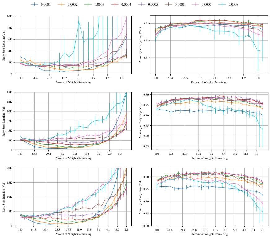
Figure 32: The early-stopping iteration and validation accuracy at that iteration of the iterative lottery ticket experiment on the Conv-2 (top), Conv-4 (middle), and Conv-6 (bottom) architectures trained using the Adam optimizer at various learning rates. Each line represents a different learning rate.

图 32：在用各种学习率的 Adam 优化器训练的 Conv-2（上）、Conv-4（中）和 Conv-6（下）结构上，迭代彩票实验的早停迭代以及该迭代上的验证精度。每条线代表一种不同的学习率。

Here, we select the learning rate that we use for Adam in the main body of the paper. Our criteria for selecting the learning rate are the same as in Appendix G: minimizing training iterations and maximizing accuracy at early-stopping, finding winning tickets containing as few parameters as possible, and remaining conservative enough to apply to a range of other experiments.

这里，我们选择正文中为 Adam 使用的学习率。我们选择学习率的准则与附录 G 相同：最小化训练迭代并最大化早停时的精度，找到包含尽可能少参数的中奖彩票，并保持足够保守以便适用于一系列其他实验。

Figure 32 shows the results of performing the iterative lottery ticket experiment on the Conv-2 (top), Conv-4 (middle), and Conv-6 (bottom) architectures. Since we have not yet selected the pruning rates for each network, we temporarily pruned fully-connected layers at 20% per iteration, convolutional layers at 10% per iteration, and the output layer at 10% per iteration; we explore this part of the hyperparameter space in a later subsection.

图 32 展示在 Conv-2（上）、Conv-4（中）和 Conv-6（下）结构上进行迭代彩票实验的结果。由于我们尚未为每个网络选择剪枝率，我们暂时以每轮 20% 对全连接层剪枝、以每轮 10% 对卷积层剪枝、以每轮 10% 对输出层剪枝；我们在后面的小节中探索超参数空间的这一部分。

For Conv-2, we select a learning rate of 0.0002, which has the highest initial validation accuracy, maintains both high validation accuracy and low early-stopping times for the among the longest, and reaches the fastest early-stopping times. This learning rate also leads to a 3.3 percentage point improvement in validation accuracy when the network is pruned to 3% of its original size. Other learning rates, such 0.0004, have lower initial validation accuracy (65.2% vs 67.6%) but eventually reach higher absolute levels of validation accuracy (71.7%, a 6.5 percentage point increase, vs. 70.9%, a 3.3 percentage point increase). However, learning rate 0.0002 shows the highest proportional decrease in early-stopping times: 4.8x (when pruned to 8.8% of the original network size).

对 Conv-2，我们选择学习率 0.0002，它具有最高的初始验证精度，把高验证精度和低早停时间保持得最久之列，并达到最快的早停时间。当网络被剪到原规模的 3% 时，这一学习率还带来 3.3 个百分点的验证精度提升。其他学习率，例如 0.0004，初始验证精度更低（65.2% 对 67.6%），但最终达到更高的绝对验证精度水平（71.7%，提高 6.5 个百分点，对 70.9%，提高 3.3 个百分点）。不过，学习率 0.0002 显示出最高比例的早停时间下降：4.8 倍（当剪到原网络规模的 8.8% 时）。

For Conv-4, we select learning rate 0.0003, which has among the highest initial validation accuracy, maintains high validation accuracy and fast early-stopping times when pruned by among the most, and balances improvements in validation accuracy (3.7 percentage point improvement to 78.6% when 5.4% of weights remain) and improvements in early-stopping time (4.27x when 11.1% of weights remain). Other learning rates reach higher validation accuracy (0.0004—3.6 percentage point improvement to 79.1% accuracy when 5.4% of weights remain) or show better improvements in early-stopping times (0.0002—5.1x faster when 9.2% of weights remain) but not both.

对 Conv-4，我们选择学习率 0.0003，它的初始验证精度属于最高之列，在被剪得最多时仍能保持高验证精度和很快的早停时间，并在验证精度提升（剩余 5.4% 权重时提高 3.7 个百分点至 78.6%）与早停时间提升（剩余 11.1% 权重时快 4.27 倍）之间取得平衡。其他学习率达到更高验证精度（0.0004——剩余 5.4% 权重时提高 3.6 个百分点至 79.1%）或在早停时间上有更好提升（0.0002——剩余 9.2% 权重时快 5.1 倍），但不能两者兼得。

For Conv-6, we also select learning rate 0.0003 for similar reasons to those provided for Conv-4. Validation accuracy improves by 2.4 percentage points to 81.5% when 9.31% of weights remain and early-stopping times improve by 2.61x when pruned to 11.9%. Learning rate 0.0004 reaches high final validation accuracy (81.9%, an increase of 2.7 percentage points, when 15.2% of weights remain) but with smaller improvements in early-stopping times, and learning rate 0.0002 shows greater improvements in early-stopping times (6.26x when 19.7% of weights remain) but reaches lower overall validation accuracy.

对 Conv-6，出于与 Conv-4 类似的理由，我们也选择学习率 0.0003。当剩余 9.31% 的权重时，验证精度提高 2.4 个百分点至 81.5%；当剪到 11.9% 时，早停时间改善 2.61 倍。学习率 0.0004 达到很高的最终验证精度（剩余 15.2% 权重时为 81.9%，提高 2.7 个百分点），但早停时间的改善较小；学习率 0.0002 在早停时间上有更大改善（剩余 19.7% 权重时快 6.26 倍），但达到的总体验证精度更低。

We note that, across nearly all combinations of learning rates, the lottery ticket pattern—where early-stopping times were maintain or decreased and validation accuracy was maintained or increased during the course of the lottery ticket experiment—continues to hold. This pattern fails to hold at the very highest learning rates: early-stopping times decreased only briefly (in the case of Conv-2 or Conv-4) or not at all (in the case of Conv-6), and accuracy increased only briefly (in the case of all three networks). This pattern is similar to that which we observe in Section 4: at the highest learning rates, our iterative pruning algorithm fails to find winning tickets.

我们注意到，在几乎所有学习率组合上，彩票模式——即在彩票实验过程中早停时间得以保持或下降、验证精度得以保持或上升——继续成立。这一模式在非常高的学习率下不再成立：早停时间只短暂下降（对 Conv-2 或 Conv-4）或完全不下降（对 Conv-6），精度也只短暂上升（对所有三个网络）。这一模式类似于我们在第 4 节中观察到的：在最高学习率下，我们的迭代剪枝算法找不到中奖彩票。

H.3 Other Optimization Algorithms

H.3 其他优化算法

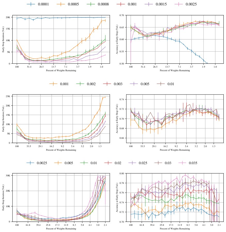
Figure 33: The early-stopping iteration and validation accuracy at that iteration of the iterative lottery ticket experiment on the Conv-2 (top), Conv-4 (middle), and Conv-6 (bottom) architectures trained using SGD at various learning rates. Each line represents a different learning rate. The legend for each pair of graphs is above the graphs.

图 33：在用各种学习率的 SGD 训练的 Conv-2（上）、Conv-4（中）和 Conv-6（下）结构上，迭代彩票实验的早停迭代以及该迭代上的验证精度。每条线代表一种不同的学习率。每对图的图例在图的上方。

H.3.1 SGD

Here, we explore the behavior of the lottery ticket experiment when the Conv-2, Conv-4, and Conv-6 networks are optimized with stochastic gradient descent (SGD) at various learning rates. The results of doing so appear in Figure 33. In general, these networks—particularly Conv-2 and Conv-4—proved challenging to train with SGD and Glorot initialization. As Figure 33 reflects, we could not find SGD learning rates for which the unpruned networks matched the validation accuracy of the same networks when trained with Adam; at best, the SGD-trained unpruned networks were typically 2-3 percentage points less accurate. At higher learning rates than those in Figure 32, gradients tended to explode when training the unpruned network; at lower learning rates, the networks often failed to learn at all.

H.3.1 SGD

这里，我们探索 Conv-2、Conv-4 和 Conv-6 网络用各种学习率的随机梯度下降（SGD）优化时彩票实验的行为。结果见图 33。总体而言，这些网络——尤其是 Conv-2 和 Conv-4——用 SGD 和 Glorot 初始化被证明很难训练。如图 33 所反映的，我们找不到这样的 SGD 学习率，能使未剪枝网络匹配同一网络用 Adam 训练时的验证精度；最好的情况下，用 SGD 训练的未剪枝网络通常精度低 2–3 个百分点。在高于图 32 中的学习率时，训练未剪枝网络时梯度往往会爆炸；在更低的学习率下，网络常常完全学不会。

At all of the learning rates depicted, we found winning tickets. In all cases, early-stopping times initially decreased with pruning before eventually increasing again, just as in other lottery ticket experiments. The Conv-6 network also exhibited the same accuracy patterns as other experiments, with validation accuracy initially increasing with pruning before eventually decreasing again.

在所展示的所有学习率上，我们都找到了中奖彩票。在所有情形中，早停时间起初随剪枝下降，随后再次上升，正如其他彩票实验一样。Conv-6 网络也表现出与其他实验相同的精度模式：验证精度起初随剪枝上升，随后再次下降。

However, the Conv-2 and Conv-4 architectures exhibited a different validation accuracy pattern from other experiments in this paper. Accuracy initially declined with pruning before rising as the network was further pruned; it eventually matched or surpassed the accuracy of the unpruned network. When they eventually did surpass the accuracy of the original network, the pruned networks reached early-stopping in about the same or fewer iterations than the original network, constituting a winning ticket by our definition. Interestingly, this pattern also appeared for Conv-6 networks at slower SGD learning rates, suggesting that faster learning rates for Conv-2 and Conv-4 than those in Figure 32 might cause the usual lottery ticket accuracy pattern to reemerge. Unfortunately, at these higher learning rates, gradients exploded on the unpruned networks, preventing us from running these experiments.

不过，Conv-2 和 Conv-4 结构表现出与本文其他实验不同的验证精度模式。精度起初随剪枝下降，然后随着网络被进一步剪枝而上升；它最终匹配或超过未剪枝网络的精度。当它们最终超过原网络精度时，被剪枝的网络大约在与原网络相同或更少的迭代内达到早停，按我们的定义构成一张中奖彩票。有意思的是，这一模式也出现在较慢 SGD 学习率下的 Conv-6 网络上，表明对 Conv-2 和 Conv-4 使用比图 32 更高的学习率，可能会使通常的彩票精度模式重新出现。可惜，在这些更高学习率下，未剪枝网络上的梯度会爆炸，使我们无法运行这些实验。

H.3.2 Momentum

Here, we explore the behavior of the lottery ticket experiment when the network is optimized with SGD with momentum (0.9) at various learning rates. The results of doing so appear in Figure 34. In general, the lottery ticket pattern continues to apply, with early-stopping times decreasing and accuracy increasing as the networks are pruned. However, there were two exceptions to this pattern:

H.3.2 动量

这里，我们探索网络用各种学习率的带动量（0.9）SGD 优化时彩票实验的行为。结果见图 34。总体而言，彩票模式继续适用：随着网络被剪枝，早停时间下降、精度上升。不过，这一模式有两个例外：

1. At the very lowest learning rates (e.g., learning rate 0.001 for Conv-4 and all but the highest learning rate for Conv-2), accuracy initially decreased before increasing to higher levels than reached by the unpruned network; this is the same pattern we observed when training these networks with SGD.

1. 在非常低的学习率下（例如 Conv-4 的学习率 0.001，以及 Conv-2 除最高学习率外的所有学习率），精度起初下降，随后上升到高于未剪枝网络所达到的水平；这与我们用 SGD 训练这些网络时观察到的模式相同。

2. At the very highest learning rates (e.g., learning rates 0.005 and 0.008 for Conv-2 and Conv-4), early-stopping times never decreased and instead remained stable before increasing; this is the same pattern we observed for the highest learning rates when training with Adam.

2. 在非常高的学习率下（例如 Conv-2 和 Conv-4 的学习率 0.005 和 0.008），早停时间从未下降，而是保持稳定随后上升；这与我们用 Adam 训练时在最高学习率下观察到的模式相同。

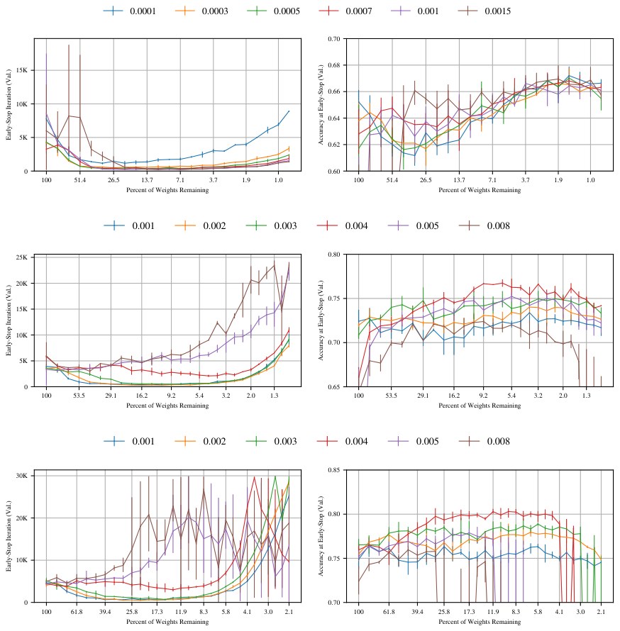
Figure 34: The early-stopping iteration and validation accuracy at that iteration of the iterative lottery ticket experiment on the Conv-2 (top), Conv-4 (middle), and Conv-6 (bottom) architectures trained using SGD with momentum (0.9) at various learning rates. Each line represents a different learning rate. The legend for each pair of graphs is above the graphs. Lines that are unstable and contain large error bars (large vertical lines) indicate that some experiments failed to learn effectively, leading to very low accuracy and very high early-stopping times; these experiments reduce the averages that the lines trace and lead to much wider error bars.

图 34：在用各种学习率的带动量（0.9）SGD 训练的 Conv-2（上）、Conv-4（中）和 Conv-6（下）结构上，迭代彩票实验的早停迭代以及该迭代上的验证精度。每条线代表一种不同的学习率。每对图的图例在图的上方。不稳定且包含很大误差条（很长的竖线）的线表明，有些实验未能有效学习，导致精度很低、早停时间很长；这些实验拉低了线所描画的平均值，并使误差条宽得多。

H.4 Iterative Pruning Rate

H.4 迭代剪枝率

For the convolutional network architectures, we select different pruning rates for convolutional and fully-connected layers. In the Conv-2 and Conv-4 architectures, convolutional parameters make up a relatively small portion of the overall number of parameters in the models. By pruning convolutions more slowly, we are likely to be able to prune the model further while maintaining performance. In other words, we hypothesize that, if all layers were pruned evenly, convolutional layers would become a bottleneck that would make it more difficult to find lower parameter-count models that are still able to learn. For Conv-6, the opposite may be true: since nearly two thirds of its parameters are in convolutional layers, pruning fully-connected layers could become the bottleneck.

对卷积网络结构，我们为卷积层和全连接层选择不同的剪枝率。在 Conv-2 和 Conv-4 结构中，卷积参数只占模型总参数量相对较小的一部分。通过更慢地剪卷积，我们更可能在保持表现的同时把模型剪得更远。换句话说，我们猜想：如果所有层被均匀剪枝，卷积层会成为瓶颈，使找到仍能学习的更低参数量模型变得更困难。对 Conv-6，相反的情况可能成立：由于近三分之二的参数在卷积层中，剪全连接层可能成为瓶颈。

Our criterion for selecting hyperparameters in this section is to find a combination of pruning rates that allows networks to reach the lowest possible parameter-counts while maintaining validation accuracy at or above the original accuracy and early-stopping times at or below that for the original network.

本节选择超参数的准则，是找到一种剪枝率组合，使网络能够达到尽可能低的参数量，同时把验证精度保持在原精度或之上，并把早停时间保持在原网络或之下。

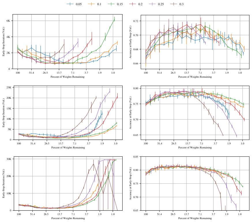
Figure 35: The early-stopping iteration and validation accuracy at that iteration of the iterative lottery ticket experiment on the Conv-2 (top), Conv-4 (middle), and Conv-6 (bottom) architectures with an iterative pruning rate of 20% for fully-connected layers. Each line represents a different iterative pruning rate for convolutional layers.

图 35：在全连接层迭代剪枝率为 20% 的 Conv-2（上）、Conv-4（中）和 Conv-6（下）结构上，迭代彩票实验的早停迭代以及该迭代上的验证精度。每条线代表卷积层的一种不同迭代剪枝率。

Figure 35 shows the results of performing the iterative lottery ticket experiment on Conv-2 (top), Conv-4 (middle), and Conv-6 (bottom) with different combinations of pruning rates.

图 35 展示在 Conv-2（上）、Conv-4（中）和 Conv-6（下）上、用不同剪枝率组合进行迭代彩票实验的结果。

According to our criteria, we select an iterative convolutional pruning rate of 10% for Conv-2, 10% for Conv-4, and 15% for Conv-6. For each network, any rate between 10% and 20% seemed reasonable. Across all convolutional pruning rates, the lottery ticket pattern continued to appear.

根据我们的准则，我们为 Conv-2 选择 10%、为 Conv-4 选择 10%、为 Conv-6 选择 15% 的迭代卷积剪枝率。对每个网络，介于 10% 和 20% 之间的任何比率看起来都合理。在所有卷积剪枝率上，彩票模式都继续出现。

H.5 Learning Rates (Dropout)

H.5 学习率（Dropout）

In order to train the Conv-2, Conv-4, and Conv-6 architectures with dropout, we repeated the exercise from Section H.2 to select appropriate learning rates. Figure 32 shows the results of performing the iterative lottery ticket experiment on Conv-2 (top), Conv-4 (middle), and Conv-6 (bottom) with dropout and Adam at various learning rates. A network trained with dropout takes longer to learn, so we trained each architecture for three times as many iterations as in the experiments without dropout: 60,000 iterations for Conv-2, 75,000 iterations for Conv-4, and 90,000 iterations for Conv-6. We iteratively pruned these networks at the rates determined in Section H.4.

为了用 dropout 训练 Conv-2、Conv-4 和 Conv-6 结构，我们重复了第 H.2 节的做法来选择合适的学习率。图 32 展示在 Conv-2（上）、Conv-4（中）和 Conv-6（下）上、用 dropout 和各种学习率的 Adam 进行迭代彩票实验的结果。用 dropout 训练的网络学得更慢，因此我们把每个结构的训练迭代增至不使用 dropout 时的三倍：Conv-2 为 60,000 次迭代，Conv-4 为 75,000 次，Conv-6 为 90,000 次。我们按第 H.4 节确定的比率对这些网络做迭代剪枝。

The Conv-2 network proved to be difficult to consistently train with dropout. The top right graph in Figure 36 contains wide error bars and low average accuracy for many learning rates, especially early in the lottery ticket experiments. This indicates that some or all of the training runs failed to learn; when they were averaged into the other results, they produced the aforementioned pattern in the graphs. At learning rate 0.0001, none of the three trials learned productively until pruned to more than 26.5%, at which point all three trials started learning. At learning rate 0.0002, some of the trials failed to learn productively until several rounds of iterative pruning had passed. At learning rate 0.0003, all three networks learned productively at every pruning level. At learning rate 0.0004, one network occasionally failed to learn. We selected learning rate 0.0003, which seemed to allow networks to learn productively most often while achieving among the highest initial accuracy.

Conv-2 网络被证明很难用 dropout 稳定地训练。图 36 右上图对许多学习率、尤其是在彩票实验早期，包含很宽的误差条和很低的平均精度。这表明部分或全部训练运行未能学会；当它们被平均进其他结果时，就在图中产生了上述模式。在学习率 0.0001 下，三次试验在被剪到超过 26.5% 之前都没有有效学习，过了这一点三次试验都开始学习。在学习率 0.0002 下，部分试验直到经过若干轮迭代剪枝才开始有效学习。在学习率 0.0003 下，三个网络在每个剪枝水平上都有效学习。在学习率 0.0004 下，有一个网络偶尔未能学会。我们选择学习率 0.0003，它似乎最经常让网络有效学习，同时达到属于最高之列的初始精度。

It is interesting to note that networks that were unable to learn at a particular learning rate (for example, 0.0001) eventually began learning after several rounds of the lottery ticket experiment (that is, training, pruning, and resetting repeatedly). It is worth investigating whether this phenomenon was entirely due to pruning (that is, removing any random collection of weights would put the network in a configuration more amenable to learning) or whether training the network provided useful information for pruning, even if the network did not show improved accuracy.

值得注意的是，那些在某一学习率（例如 0.0001）下无法学习的网络，在经过若干轮彩票实验（也就是反复训练、剪枝并重置）之后最终开始学习。值得研究的是：这一现象是否完全由剪枝造成（也就是去掉任何随机的权重组都会把网络置于更便于学习的配置），还是训练网络为剪枝提供了有用信息，即便网络并没有显示出精度提升。

For both the Conv-4 and Conv-6 architectures, a slightly slower learning rate (0.0002 as opposed to 0.0003) leads to the highest accuracy on the unpruned networks in addition to the highest sustained accuracy and fastest sustained learning as the networks are pruned during the lottery ticket experiment.

对 Conv-4 和 Conv-6 结构，略慢的学习率（0.0002 而不是 0.0003）在未剪枝网络上带来最高精度，并且随着网络在彩票实验中被剪枝，也带来最高的持续精度和最快的持续学习。

With dropout, the unpruned Conv-4 architecture reaches an average validation accuracy of 77.6%, a 2.7 percentage point improvement over the unpruned Conv-4 network trained without dropout and one percentage point lower than the highest average validation accuracy attained by a winning ticket. The dropout-trained winning tickets reach 82.6% average validation accuracy when pruned to 7.6%. Early-stopping times improve by up to 1.58x (when pruned to 7.6%), a smaller improvement than then 4.27x achieved by a winning ticket obtained without dropout.

使用 dropout 时，未剪枝的 Conv-4 结构达到平均验证精度 77.6%，比不使用 dropout 训练的未剪枝 Conv-4 网络高 2.7 个百分点，比一张中奖彩票达到的最高平均验证精度低一个百分点。用 dropout 训练的中奖彩票在被剪到 7.6% 时达到平均验证精度 82.6%。早停时间最多改善 1.58 倍（当剪到 7.6% 时），小于不使用 dropout 得到的中奖彩票所达到的 4.27 倍。

With dropout, the unpruned Conv-6 architecture reaches an average validation accuracy of 81.3%, an improvement of 2.2 percentage points over the accuracy without dropout; this nearly matches the 81.5% average accuracy obtained by Conv-6 trained without dropout and pruned to 9.31%. The dropout-trained winning tickets further improve upon these numbers, reaching 84.8% average validation accuracy when pruned to 10.5%. Improvements in early-stopping times are less dramatic than without dropout: a 1.5x average improvement when the network is pruned to 15.1%.

使用 dropout 时，未剪枝的 Conv-6 结构达到平均验证精度 81.3%，比不使用 dropout 时的精度高 2.2 个百分点；这几乎匹配不使用 dropout、被剪到 9.31% 的 Conv-6 所获得的 81.5% 平均精度。用 dropout 训练的中奖彩票进一步改进这些数字，在被剪到 10.5% 时达到平均验证精度 84.8%。早停时间的改善不如不使用 dropout 时显著：当网络被剪到 15.1% 时平均改善 1.5 倍。

At all learning rates we tested, the lottery ticket pattern generally holds for accuracy, with improvements as the networks are pruned. However, not all learning rates show the decreases in early-stopping times. To the contrary, none of the learning rates for Conv-2 show clear improvements in early-stopping times as seen in the other lottery ticket experiments. Likewise, the faster learning rates for Conv-4 and Conv-6 maintain the original early-stopping times until pruned to about 40%, at which point early-stopping times steadily increase.

在我们测试的所有学习率上，彩票模式对精度大体成立，随着网络被剪枝而有所改进。不过，并非所有学习率都显示出早停时间的下降。相反，Conv-2 的学习率没有一个像其他彩票实验那样清晰地改善早停时间。同样，Conv-4 和 Conv-6 更快的学习率把原来的早停时间保持到大约被剪到 40%，过了这一点早停时间稳步上升。

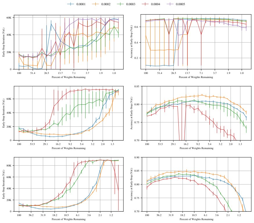
Figure 36: The early-stopping iteration and validation accuracy at that iteration of the iterative lottery ticket experiment on the Conv-2 (top), Conv-4 (middle), and Conv-6 (bottom) architectures trained using dropout and the Adam optimizer at various learning rates. Each line represents a different learning rate.

图 36：在用 dropout 和各种学习率的 Adam 优化器训练的 Conv-2（上）、Conv-4（中）和 Conv-6（下）结构上，迭代彩票实验的早停迭代以及该迭代上的验证精度。每条线代表一种不同的学习率。

H.6 Pruning Convolutions vs. Pruning Fully-Connected Layers

H.6 剪卷积与剪全连接层

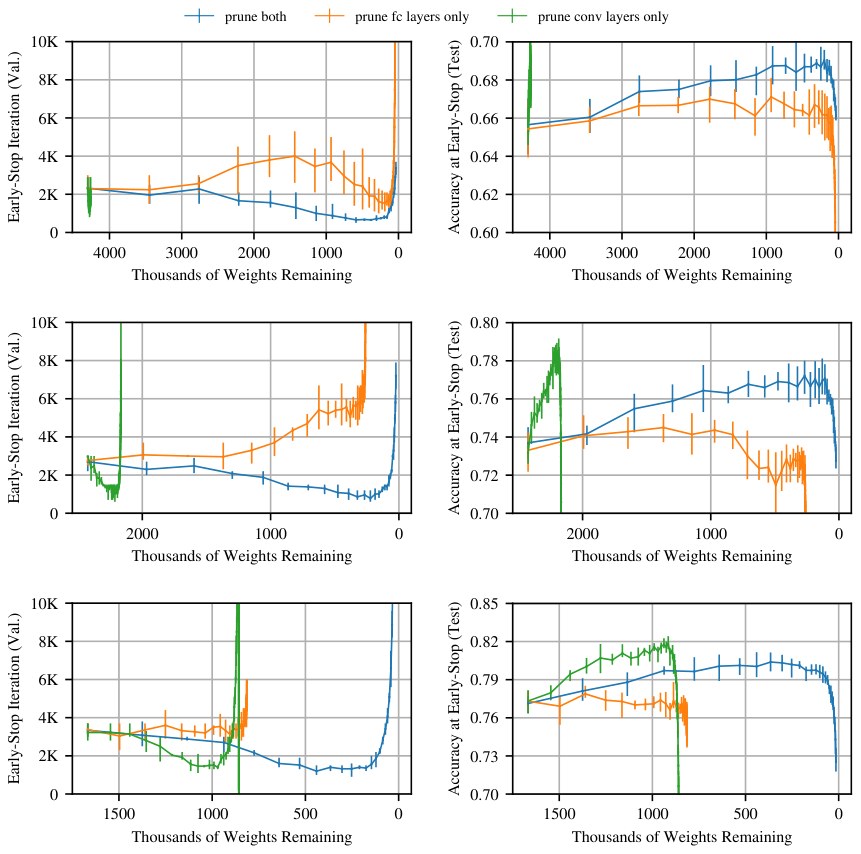
Figure 37: Early-stopping iteration and accuracy of the Conv-2 (top), Conv-4 (middle), and Conv-6 (bottom) networks when only convolutions are pruned, only fully-connected layers are pruned, and both are pruned. The x-axis measures the number of parameters remaining, making it possible to see the relative contributions to the overall network made by pruning FC layers and convolutions individually.

图 37：只剪卷积、只剪全连接层、以及两者都剪时，Conv-2（上）、Conv-4（中）和 Conv-6（下）网络的早停迭代与精度。x 轴度量剩余参数数量，从而可以看出分别剪全连接层和卷积对整个网络的相对贡献。

Figure 37 shows the effect of pruning convolutions alone (green), fully-connected layers alone (orange) and pruning both (blue). The x-axis measures the number of parameters remaining to emphasize the relative contributions made by pruning convolutions and fully-connected layers to the overall network. In all three cases, pruning convolutions alone leads to higher test accuracy and faster learning; pruning fully-connected layers alone generally causes test accuracy to worsen and learning to slow. However, pruning convolutions alone has limited ability to reduce the overall parameter-count of the network, since fully-connected layers comprise 99%, 89%, and 35% of the parameters in Conv-2, Conv-4, and Conv-6.

图 37 展示只剪卷积（绿）、只剪全连接层（橙）以及两者都剪（蓝）的效果。x 轴度量剩余参数数量，以强调剪卷积和剪全连接层对整个网络的相对贡献。在所有三种情形中，只剪卷积会带来更高的测试精度和更快的学习；只剪全连接层通常会使测试精度变差、学习变慢。不过，只剪卷积减少网络总参数量的能力有限，因为全连接层分别占 Conv-2、Conv-4 和 Conv-6 参数的 99%、89% 和 35%。

Appendix I Hyperparameter Exploration for VGG-19 and Resnet-18 on CIFAR10

附录 I CIFAR10 上 VGG-19 与 Resnet-18 的超参数探索

This Appendix accompanies the VGG-19 and Resnet-18 experiments in Section 4. It details the pruning scheme, training regimes, and hyperparameters that we use for these networks.

本附录配合第 4 节中的 VGG-19 和 Resnet-18 实验。它详细说明我们为这些网络使用的剪枝方案、训练制度与超参数。

I.1 Global Pruning

I.1 全局剪枝

In our experiments with the Lenet and Conv-2/4/6 architectures, we separately prune a fraction of the parameters in each layer (layer-wise pruning). In our experiments with VGG-19 and Resnet-18, we instead prune globally; that is, we prune all of the weights in convolutional layers collectively without regard for the specific layer from which any weight originated.

在 Lenet 和 Conv-2/4/6 结构的实验中，我们分别剪掉每一层中一部分参数（逐层剪枝）。在 VGG-19 和 Resnet-18 的实验中，我们改为全局剪枝；也就是说，我们把卷积层中的所有权重集体剪枝，而不考虑任何权重来自哪一层。

Figures 38 (VGG-19) and 39 (Resnet-18) compare the winning tickets found by global pruning (solid lines) and layer-wise pruning (dashed lines) for the hyperparameters from Section 4. When training VGG-19 with learning rate 0.1 and warmup to iteration 10,000, we find winning tickets when $P_{m}\geq 6.9\%$ for layer-wise pruning vs. $P_{m}\geq 1.5\%$ for global pruning. For other hyperparameters, accuracy similarly drops off when sooner for layer-wise pruning than for global pruning. Global pruning also finds smaller winning tickets than layer-wise pruning for Resnet-18, but the difference is less extreme than for VGG-19.

图 38（VGG-19）和图 39（Resnet-18）比较了用第 4 节超参数时，全局剪枝（实线）和逐层剪枝（虚线）找到的中奖彩票。当用学习率 0.1 并对 VGG-19 预热到第 10,000 次迭代时，逐层剪枝在 $P_{m}\geq 6.9\%$ 时找到中奖彩票，全局剪枝则在 $P_{m}\geq 1.5\%$ 时找到。对其它超参数，精度同样在逐层剪枝时比全局剪枝更早掉下去。全局剪枝也为 Resnet-18 找到比逐层剪枝更小的中奖彩票，但差别不像 VGG-19 那样极端。

In Section 4, we discuss the rationale for the efficacy of global pruning on deeper networks. In summary, the layers in these deep networks have vastly different numbers of parameters (particularly severely so for VGG-19); if we prune layer-wise, we conjecture that layers with fewer parameters become bottlenecks on our ability to find smaller winning tickets.

在第 4 节中，我们讨论了全局剪枝在更深网络上有效的理由。概括地说，这些深网络中各层的参数数量差异巨大（对 VGG-19 尤其严重）；如果我们逐层剪枝，我们猜想参数更少的层会成为找到更小中奖彩票的瓶颈。

Regardless of whether we use layer-wise or global pruning, the patterns from Section 4 hold: at learning rate 0.1, iterative pruning finds winning tickets for neither network; at learning rate 0.01, the lottery ticket pattern reemerges; and when training with warmup to a higher learning rate, iterative pruning finds winning tickets. Figures 40 (VGG-19) and 41 (Resnet-18) present the same data as Figures 7 (VGG-19) and 8 (Resnet-18) from Section 4 with layer-wise pruning rather than global pruning. The graphs follow the same trends as in Section 4, but the smallest winning tickets are larger than those found by global pruning.

无论我们使用逐层还是全局剪枝，第 4 节中的模式都成立：在学习率 0.1 下，迭代剪枝对两个网络都找不到中奖彩票；在学习率 0.01 下，彩票模式重新出现；当预热到更高学习率训练时，迭代剪枝能找到中奖彩票。图 40（VGG-19）和图 41（Resnet-18）给出与第 4 节图 7（VGG-19）和图 8（Resnet-18）相同的数据，只是用逐层剪枝而不是全局剪枝。这些图遵循与第 4 节相同的趋势，但找到的最小中奖彩票比全局剪枝找到的更大。

I.2 VGG-19 Details

I.2 VGG-19 细节

The VGG19 architecture was first designed by Simonyan & Zisserman (2014) for Imagenet. The version that we use here was adapted by Liu et al. (2019) for CIFAR10. The network is structured as described in Figure 2: it has five groups of 3x3 convolutional layers, the first four of which are followed by max-pooling (stride 2) and the last of which is followed by average pooling. The network has one final dense layer connecting the result of the average-pooling to the output.

VGG19 结构最初由 Simonyan 与 Zisserman（2014）为 Imagenet 设计。我们这里使用的版本由 Liu 等人（2019）为 CIFAR10 改编。网络结构如图 2 所述：它有五组 3x3 卷积层，前四组之后是最大池化（步幅 2），最后一组之后是平均池化。网络有一个最终的稠密层，把平均池化的结果连到输出。

We largely follow the training procedure for resnet18 described in Appendix I:

我们大体遵循附录 I 中描述的 resnet18 训练程序：

• • We use the same train/test/validation split.

• • 我们使用相同的训练/测试/验证划分。

• • We use the same data augmentation procedure.

• • 我们使用相同的数据增强程序。

• • We use a batch size of 64.

• • 我们使用批次大小 64。

• • We use batch normalization.

• • 我们使用批归一化。

• • We use a weight decay of 0.0001.

• • 我们使用 0.0001 的权重衰减。

• • We use three stages of training at decreasing learning rates. We train for 160 epochs (112,480 iterations), decreasing the learning rate by a factor of ten after 80 and 120 epochs.

• • 我们使用三个阶段、学习率递减的训练。我们训练 160 个周期（112,480 次迭代），并在第 80 和 120 个周期后把学习率降为原来的十分之一。

• • We use Gaussian Glorot initialization.

• • 我们使用高斯 Glorot 初始化。

We globally prune the convolutional layers of the network at a rate of 20% per iteration, and we do not prune the 5120 parameters in the output layer.

我们以每轮 20% 的比率全局剪枝网络的卷积层，并且不剪输出层中的 5120 个参数。

Liu et al. (2019) uses an initial pruning rate of 0.1. We train VGG19 with both this learning rate and a learning rate of 0.01.

Liu 等人（2019）使用 0.1 的初始剪枝率。我们同时用这一学习率和 0.01 的学习率训练 VGG19。

I.3 Resnet-18 Details

I.3 Resnet-18 细节

The Resnet-18 architecture was first introduced by He et al. (2016). The architecture comprises 20 total layers as described in Figure 2: a convolutional layer followed by nine pairs of convolutional layers (with residual connections around the pairs), average pooling, and a fully-connected output layer.

Resnet-18 结构最初由 He 等人（2016）提出。该结构如图 2 所述共有 20 层：一个卷积层，后接九对卷积层（对周围有残差连接），再接平均池化和一个全连接输出层。

We follow the experimental design of He et al. (2016):

我们遵循 He 等人（2016）的实验设计：

• • We divide the training set into 45,000 training examples and 5,000 validation examples. We use the validation set to select hyperparameters in this appendix and the test set to evaluate in Section 4.

• • 我们把训练集分成 45,000 个训练样本和 5,000 个验证样本。我们用验证集在本附录中选择超参数，用测试集在第 4 节中评估。

• • We augment training data using random flips and random four pixel pads and crops.

• • 我们用随机翻转以及随机四像素填充与裁剪来增强训练数据。

• • We use a batch size of 128.

• • 我们使用批次大小 128。

• • We use batch normalization.

• • 我们使用批归一化。

• • We use weight decay of 0.0001.

• • 我们使用 0.0001 的权重衰减。

• • We train using SGD with momentum (0.9).

• • 我们用带动量（0.9）的 SGD 训练。

• • We use three stages of training at decreasing learning rates. Our stages last for 20,000, 5,000, and 5,000 iterations each, shorter than the 32,000, 16,000, and 16,000 used in He et al. (2016). Since each of our iterative pruning experiments requires training the network 15-30 times consecutively, we select this abbreviated training schedule to make it possible to explore a wider range of hyperparameters.

• • 我们使用三个阶段、学习率递减的训练。我们的各阶段分别持续 20,000、5,000 和 5,000 次迭代，短于 He 等人（2016）所用的 32,000、16,000 和 16,000。由于每一次迭代剪枝实验都需要把网络连续训练 15–30 次，我们选择这一缩短的训练日程，以便能够探索更广的超参数范围。

• • We use Gaussian Glorot initialization.

• • 我们使用高斯 Glorot 初始化。

We globally prune convolutions at a rate of 20% per iteration. We do not prune the 2560 parameters used to downsample residual connections or the 640 parameters in the fully-connected output layer, as they comprise such a small portion of the overall network.

我们以每轮 20% 的比率全局剪枝卷积。我们不剪用于对残差连接下采样的 2560 个参数，也不剪全连接输出层中的 640 个参数，因为它们只占整个网络很小一部分。

I.4 Learning Rate

I.4 学习率

In Section 4, we observe that iterative pruning is unable to find winning tickets for VGG-19 and Resnet-18 at the typical, high learning rate used to train the network (0.1) but it is able to do so at a lower learning rate (0.01). Figures 42 and 43 explore several other learning rates. In general, iterative pruning cannot find winning tickets at any rate above 0.01 for either network; for higher learning rates, the pruned networks with the original initialization perform no better than when randomly reinitialized.

在第 4 节中，我们观察到：迭代剪枝无法在训练网络所用的典型高学习率（0.1）下为 VGG-19 和 Resnet-18 找到中奖彩票，但在更低学习率（0.01）下能够做到。图 42 和图 43 探索了若干其他学习率。总体而言，迭代剪枝在两个网络上、对任何高于 0.01 的学习率都找不到中奖彩票；对更高学习率，带原来初始化的被剪枝网络并不比随机重新初始化时表现更好。

I.5 Warmup Iteration

I.5 预热迭代

In Section 4, we describe how adding linear warmup to the initial learning rate makes it possible to find winning tickets for VGG-19 and Resnet-18 at higher learning rates (and, thereby, winning tickets that reach higher accuracy). In Figures 44 and 45, we explore the number of iterations $k$ over which warmup should occur.

在第 4 节中，我们描述了如何给初始学习率加上线性预热，使得能够在更高学习率下为 VGG-19 和 Resnet-18 找到中奖彩票（从而找到达到更高精度的中奖彩票）。在图 44 和图 45 中，我们探索预热应当发生的迭代次数 $k$。

For VGG-19, we were able to find values of $k$ for which iterative pruning could identify winning tickets when the network was trained at the original learning rate (0.1). For Resnet-18, warmup made it possible to increase the learning rate from 0.01 to 0.03, but no further. When exploring values of $k$, we therefore us learning rate 0.1 for VGG-19 and 0.03 for Resnet-18.

对 VGG-19，我们能够找到这样的 $k$ 值，使迭代剪枝能在网络以原来的学习率（0.1）训练时识别出中奖彩票。对 Resnet-18，预热使得能够把学习率从 0.01 提高到 0.03，但不能再高。因此在探索 $k$ 的取值时，我们对 VGG-19 使用学习率 0.1，对 Resnet-18 使用 0.03。

In general, the greater the value of $k$, the higher the accuracy of the eventual winning tickets.

总体而言，$k$ 越大，最终中奖彩票的精度越高。

Resnet-18.

For values of $k$ below 5000, accuracy improves rapidly as $k$ increases. This relationship reaches a point of diminishing returns above $k=5000$. For the experiments in Section 4, we select $k=20000$, which achieves the highest validation accuracy.

Resnet-18。

对低于 5000 的 $k$ 值，精度随着 $k$ 增大而迅速提高。这一关系在 $k=5000$ 以上到达收益递减的点。对第 4 节中的实验，我们选择 $k=20000$，它达到最高的验证精度。

VGG-19.

For values of $k$ below 5000, accuracy improves rapidly as $k$ increases. This relationship reaches a point of diminishing returns above $k=5000$. For the experiments in Section 4, we select $k=10000$, as there is little benefit to larger values of $k$.

VGG-19。

对低于 5000 的 $k$ 值，精度随着 $k$ 增大而迅速提高。这一关系在 $k=5000$ 以上到达收益递减的点。对第 4 节中的实验，我们选择 $k=10000$，因为更大的 $k$ 值收益很小。

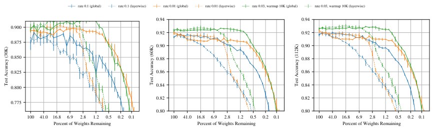
Figure 38: Validation accuracy (at 30K, 60K, and 112K iterations) of VGG-19 when iteratively pruned with global (solid) and layer-wise (dashed) pruning.

图 38：VGG-19 在用全局（实线）和逐层（虚线）剪枝做迭代剪枝时（于 30K、60K 和 112K 次迭代）的验证精度。

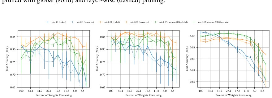
Figure 39: Validation accuracy (at 10K, 20K, and 30K iterations) of Resnet-18 when iteratively pruned with global (solid) and layer-wise (dashed) pruning.

图 39：Resnet-18 在用全局（实线）和逐层（虚线）剪枝做迭代剪枝时（于 10K、20K 和 30K 次迭代）的验证精度。

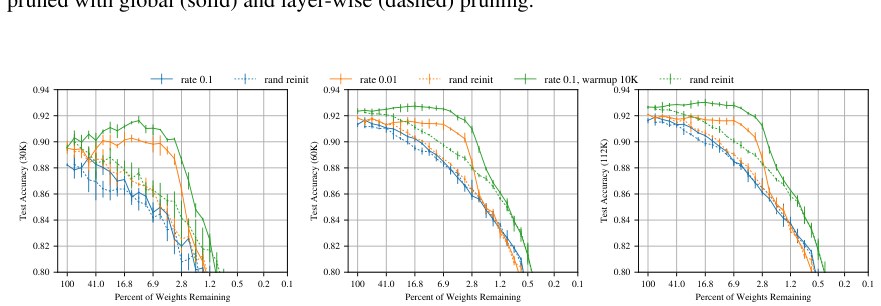
Figure 40: Test accuracy (at 30K, 60K, and 112K iterations) of VGG-19 when iteratively pruned with layer-wise pruning. This is the same as Figure 7, except with layer-wise pruning rather than global pruning.

图 40：VGG-19 在用逐层剪枝做迭代剪枝时（于 30K、60K 和 112K 次迭代）的测试精度。这与图 7 相同，只是用逐层剪枝而不是全局剪枝。

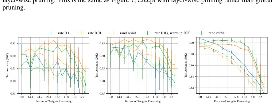
Figure 41: Test accuracy (at 10K, 20K, and 30K iterations) of Resnet-18 when iteratively pruned with layer-wise pruning. This is the same as Figure 8 except with layer-wise pruning rather than global pruning.

图 41：Resnet-18 在用逐层剪枝做迭代剪枝时（于 10K、20K 和 30K 次迭代）的测试精度。这与图 8 相同，只是用逐层剪枝而不是全局剪枝。

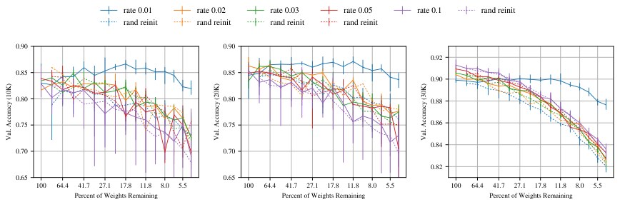
Figure 42: Validation accuracy (at 10K, 20K, and 30K iterations) of Resnet-18 when iteratively pruned and trained with various learning rates.

图 42：Resnet-18 在迭代剪枝并用各种学习率训练时（于 10K、20K 和 30K 次迭代）的验证精度。

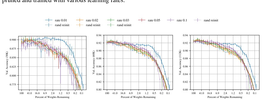
Figure 43: Validation accuracy (at 30K, 60K, and 112K iterations) of VGG-19 when iteratively pruned and trained with various learning rates.

图 43：VGG-19 在迭代剪枝并用各种学习率训练时（于 30K、60K 和 112K 次迭代）的验证精度。

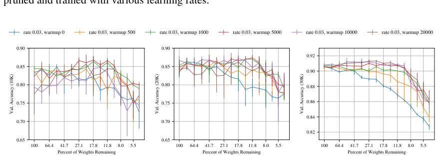
Figure 44: Validation accuracy (at 10K, 20K, and 30K iterations) of Resnet-18 when iteratively pruned and trained with varying amounts of warmup at learning rate 0.03.

图 44：Resnet-18 在迭代剪枝、并以学习率 0.03 用不同预热量训练时（于 10K、20K 和 30K 次迭代）的验证精度。

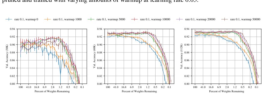
Figure 45: Validation accuracy (at 30K, 60K, and 112K iterations) of VGG-19 when iteratively pruned and trained with varying amounts of warmup at learning rate 0.1.

图 45：VGG-19 在迭代剪枝、并以学习率 0.1 用不同预热量训练时（于 30K、60K 和 112K 次迭代）的验证精度。