Look, Listen and Learn
Look, Listen and Learn
Look, Listen and Learn:看、听与学
Abstract
摘要
We consider the question: what can be learnt by looking at and listening to a large number of unlabelled videos? There is a valuable, but so far untapped, source of information contained in the video itself – the correspondence between the visual and the audio streams, and we introduce a novel “Audio-Visual Correspondence” learning task that makes use of this. Training visual and audio networks from scratch, without any additional supervision other than the raw unconstrained videos themselves, is shown to successfully solve this task, and, more interestingly, result in good visual and audio representations. These features set the new state-of-the-art on two sound classification benchmarks, and perform on par with the state-of-the-art self-supervised approaches on ImageNet classification. We also demonstrate that the network is able to localize objects in both modalities, as well as perform fine-grained recognition tasks.
我们考虑这样一个问题:只看、只听大量未标注视频,能够学到什么?视频本身含有一种很有价值、却尚未被充分利用的信息——视觉流与音频流之间的对应,我们据此提出一种新的“音视对应”(Audio-Visual Correspondence)学习任务。结果表明,除原始的、不受约束的视频本身外不再使用任何额外监督,从零训练视觉和音频网络,不仅能成功完成这一任务,更有意思的是还能得到很好的视觉和音频表征。这些特征在两项声音分类基准上刷新了最好成绩,并在 ImageNet 分类上与当时最先进的自监督方法相当。我们还展示,网络能够在两个模态中定位物体,并能完成细粒度识别任务。
1. Introduction
1. 引言
Visual and audio events tend to occur together; not always but often: the movement of fingers and sound of the instrument when a piano, guitar or drum is played; lips moving and speech when talking; cars moving and engine noise when observing a street. The visual and audio events are concurrent in these cases because there is a common cause. In this paper we investigate whether we can use this simple observation to learn about the world both visually and aurally by simply watching and listening to videos.
视觉事件和音频事件往往一起出现,虽非总是如此,却很常见:弹钢琴、吉他或打鼓时,手指的动作与乐器的声音;说话时,嘴唇的动作与语音;看街道时,车辆的移动与引擎声。这些情形里视听事件同时发生,是因为有共同的原因。本文考察能否利用这一简单观察,仅仅通过观看和聆听视频,同时从视觉和听觉上认识世界。
We ask the question: what can be learnt by training visual and audio networks simultaneously to predict whether visual information (a video frame) corresponds or not to audio information (a sound snippet)? This is a looser requirement than that the visual and audio events occur in sync. It only requires that there is something in the image that correlates with something in the audio clip – a car present in the video frame, for instance, correlating with engine noise; or an exterior shot with the sound of wind.
我们提出的问题是:同时训练视觉和音频网络,去判断视觉信息(一帧视频)与音频信息(一小段声音)是否对应,能够学到什么?这比要求视听事件精确同步更松:只需图像中有某样东西与音频片段中的某样东西相关——例如视频帧里出现汽车,与引擎声相关;或室外镜头与风声相关。
Our motivation for this work is three fold: first, as in many recent self-supervision tasks [1, 7, 9, 21, 22, 25, 35, 36], it is interesting to learn from a virtually infinite source of free supervision (video with visual and audio modes in this case) rather than requiring strong supervision; second, this is a possible source of supervision that an infant could use as their visual and audio capabilities develop; third, we want to know what can be learnt, and how well the networks are trained, for example in the performance of the visual and audio networks for other tasks.
我们做这项工作有三重动机:第一,与许多近期的自监督任务 [1, 7, 9, 21, 22, 25, 35, 36] 一样,从几乎无穷的免费监督(这里是同时带有视觉和音频模态的视频)中学习,而不依赖强监督,本身就很有意思;第二,这可能是婴儿在视觉和听觉能力发展过程中可以利用的一种监督;第三,我们想知道能学到什么、网络训得有多好,例如视觉和音频网络在其他任务上的表现。
Of course, we are not the first to make the observation that visual and audio events co-occur, and to use their concurrence or correlation as supervision for training a network. In a series of recent and inspiring papers [3, 12, 23, 24], the group at MIT has investigated precisely this. However, their goal is always to train a single network for one of the modes, for example, train a visual network to generate sounds in [23, 24]; or train an audio network to correlate with visual outputs in [3, 12], where the visual networks are pre-trained and fixed and act as a teacher. In earlier, pre deep-learning, approaches the observation was used to beautiful effect in [15] showing “pixels that sound” (e.g. for a guitar) learnt using CCA. In contrast, we train both visual and audio networks and, somewhat surprisingly, show that this is beneficial – in that our performance improves substantially over that of [3] when trained on the same data.
当然,我们并不是最早注意到视听事件会共现、并把这种同时出现或相关性当作监督来训练网络的人。MIT 的一组近期且很有启发的论文 [3, 12, 23, 24] 正是在研究这一点。不过,他们的目标始终是为其中一个模态训练单个网络:例如在 [23, 24] 中训练视觉网络来生成声音;或在 [3, 12] 中训练音频网络去与视觉输出相关,其中视觉网络是预训练并固定的,充当老师。在更早的、深度学习之前的工作里,[15] 用 CCA 学到了“会发声的像素”(例如吉他),效果非常漂亮。与之不同,我们同时训练视觉和音频网络,并且——有些出人意料地——表明这样做是有益的:在相同数据上训练时,我们的性能比 [3] 有大幅提升。
In summary: our goal is to design a system that is able to learn both visual and audio semantic information in a completely unsupervised manner by simply looking at and listening to a large number of unlabelled videos. To achieve this we introduce a novel Audio-Visual Correspondence (AVC) learning task that is used to train the two (visual and audio) networks from scratch. This task is described in section 2, together with the network architecture and training procedure. In section 3 we describe what semantic information has been learnt, and assess the performance of the audio and visual networks. We find, which we had not anticipated, that this task leads to quite fine grained visual and audio discrimination, e.g. into different instruments. In terms of quantitative performance, the audio network exceed those recently trained for audio recognition using visual supervision, and the visual network has similar performance to those trained for other, purely visual, self-supervision tasks. Furthermore, we show, as an added benefit, that we are able to localize the source of the audio event in the video frame (and also localize the corresponding regions of the sound source) using activation visualization.
总之:我们的目标是设计一个系统,只需观看和聆听大量未标注视频,就能以完全无监督的方式同时学到视觉和音频语义信息。为此我们提出一种新的音视对应(AVC)学习任务,用来从零训练这两个(视觉和音频)网络。第 2 节描述该任务以及网络结构和训练流程。第 3 节说明学到了哪些语义信息,并评测音频和视觉网络的表现。我们并未预先料到,这一任务会带来相当细粒度的视听分辨,例如区分不同乐器。在定量性能上,音频网络超过了近期借助视觉监督训练的音频识别网络,视觉网络则与为其他纯视觉自监督任务训练的网络表现相近。此外,作为额外收益,我们展示可以用激活可视化,在视频帧中定位音频事件的来源(也能定位声源所对应的区域)。
In terms of prior work, the most closely related deep learning approach that we know of is ‘SyncNet’ in [6]. However, [6] is aimed at learning to synchronize lip-regions and speech for lip-reading, rather than the more general video and audio material considered here for learning semantic representations. More generally, the AVC task is a form of co-training [5], where there are two ‘views’ of the data, and each view provides complementary information. In our case the two views are visual and audio (and each can determine semantic information independently). A similar scenario arises when the two views are visual and language (text) as in [10, 19, 32] where a common embedding is learnt. However, usually one (or both) of the networks (for images and text) are pre-trained, in contrast to the approach taken here where no supervision is required and both networks are trained from scratch.
就先前工作而言,据我们所知最接近的深度学习方法是 [6] 中的 SyncNet。不过 [6] 的目标是为唇读学习唇部区域与语音的同步,而不是本文这种更一般的视频和音频材料,用以学习语义表征。更一般地说,AVC 任务是一种协同训练(co-training)[5]:数据有两个“视图”,每个视图提供互补信息。在我们这里,两个视图是视觉和音频(并且各自都能独立判定语义信息)。类似情形也出现在两个视图分别是视觉和语言(文本)时,如 [10, 19, 32] 学习共同嵌入。不过那些工作通常会预训练图像或文本网络中的一个(或两个),与本文无需监督、两个网络都从零训练的做法不同。
2. Audio-visual correspondence learning
2. 音视对应学习
The core idea is to use a valuable but so far untapped source of information contained in the video itself – the correspondence between visual and audio streams available by virtue of them appearing together at the same time in the same video. By seeing and hearing many examples of a person playing a violin and examples of a dog barking, and never, or at least very infrequently, seeing a violin being played while hearing a dog bark and vice versa, it should be possible to conclude what a violin and a dog look and sound like, without ever being explicitly taught what is a violin or a dog.
核心想法是利用视频本身所含、迄今尚未被充分开发的信息:视觉流和音频流因同时出现在同一视频中而形成的对应。看过、听过许多有人拉小提琴的例子和狗叫的例子,又几乎从未(至少极少)在听到狗叫时看到有人拉小提琴,反过来也一样,就应当能够推断小提琴和狗看起来、听起来是什么样,而无需被人明确教过什么是小提琴或什么是狗。
We leverage this for learning by an audio-visual correspondence (AVC) task, illustrated in Figure 1. The AVC task is a simple binary classification task: given an example video frame and a short audio clip – decide whether they correspond to each other or not. The corresponding (positive) pairs are the ones that are taken at the same time from the same video, while mismatched (negative) pairs are extracted from different videos. The only way for a system to solve this task is if it learns to detect various semantic concepts in both the visual and the audio domain. Indeed, we demonstrate in Section 3.5 that our network automatically learns relevant semantic concepts in both modalities.
我们把这一点落实为图 1 所示的音视对应(AVC)任务。AVC 是一个简单的二分类任务:给定一张视频帧和一段短音频,判断二者是否对应。对应(正)样本对取自同一视频的同一时刻,不匹配(负)样本对则取自不同视频。系统要解决这一任务,唯一的办法是学会在视觉和音频两个域里检测各种语义概念。我们在第 3.5 节确实表明,网络会自动在两个模态中学到相关的语义概念。
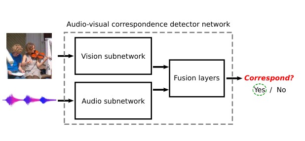
Figure 1. Audio-visual correspondence task (AVC). A network should learn to determine whether a pair of (video frame, short audio clip) correspond to each other or not. Positives are (frame, audio) extracted from the same time of one video, while negatives are a frame and audio extracted from different videos.
图 1. 音视对应任务(AVC)。网络应学会判断一对(视频帧,短音频片段)是否彼此对应。正样本是从同一视频同一时刻取出的(帧,音频),负样本则是从不同视频取出的一帧和一段音频。
It should be noted that the task is very difficult. The network is made to learn visual and audio features and concepts from scratch without ever seeing a single label. Furthermore, the AVC task itself is quite hard when done on completely unconstrained videos – videos can be very noisy, the audio source is not necessarily visible in the video (e.g. camera operator speaking, person narrating the video, sound source out of view or occluded, etc.), and the audio and visual content can be completely unrelated (e.g. edited videos with added music, very low volume sound, ambient sound such as wind dominating the audio track despite other audio events being present, etc.). Nevertheless, the results in Section 3 show that our network is able to fairly successfully solve the AVC task, and in the process learn very good visual and audio representations.
需要指出,这项任务非常困难。网络必须在从未见过任何标签的情况下,从零学习视觉和音频特征与概念。而且,在完全不受约束的视频上做 AVC 本身就很难——视频可能非常吵杂,声源不一定出现在画面里(例如摄影师在说话、有人在旁白、声源在视野外或被遮挡等),音频和视觉内容还可能完全无关(例如后期加上配乐的剪辑视频、音量极低、尽管还有其他声音事件但风声等环境声占满音轨等)。尽管如此,第 3 节的结果表明,我们的网络能够相当成功地完成 AVC 任务,并在这一过程中学到很好的视觉和音频表征。
2.1. Network architecture
2.1. 网络结构
To tackle the AVC task, we propose the network structure shown in Figure 2. It has three distinct parts: the vision and the audio subnetworks which extract visual and audio features, respectively, and the fusion network which takes these features into account to produce the final decision on whether the visual and audio signals correspond. Here we describe the three parts in more detail.
为解决 AVC 任务,我们提出图 2 所示的网络结构。它有三个不同部分:分别提取视觉和音频特征的视觉子网络与音频子网络,以及综合这些特征、最终判断视听信号是否对应的融合网络。下面更细致地描述这三部分。
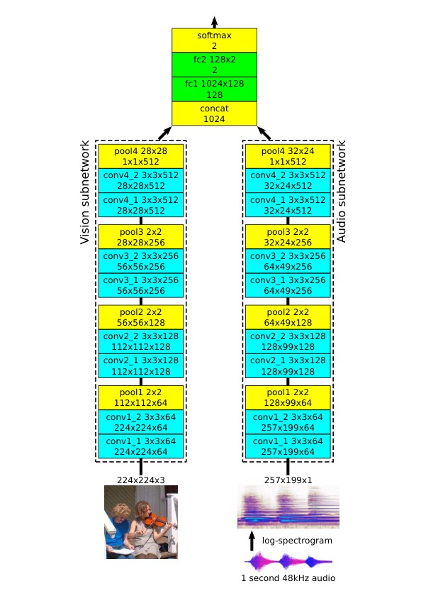
Figure 2. -Net architecture. Each blocks represents a single layer with text providing more information – first row: layer name and parameters, second row: output feature map size. Layers with a name prefix conv, pool, fc, concat, softmax are convolutional, max-pooling, fully connected, concatenation and softmax layers, respectively. The listed parameters are: conv – kernel size and number of channels, pooling – kernel size, fc – size of the weight matrix. The stride of pool layers is equal to the kernel size and there is no padding. Each convolutional layer is followed by batch normalization [13] and a ReLU nonlinearity, and the first fully connected layer (fc1) is followed by ReLU.
图 2. -Net 结构。每个块表示一层,文字给出更多信息——第一行:层名和参数,第二行:输出特征图尺寸。名称前缀为 conv、pool、fc、concat、softmax 的层,分别是卷积、最大池化、全连接、拼接和 softmax 层。所列参数为:conv——核大小与通道数,pooling——核大小,fc——权重矩阵大小。池化层的步长等于核大小,并且没有填充。每个卷积层之后接批归一化 [13] 和 ReLU 非线性,第一个全连接层(fc1)之后接 ReLU。
Vision subnetwork. The input to the vision subnetwork is a colour image. We follow the VGG-network [31] design style, with convolutional filters, and max-pooling layers with stride 2 and no padding. The network can be segmented into four blocks of conv+conv+pool layers such that inside each block the two conv layers have the same number of filters, while consecutive blocks have doubling filter numbers: 64, 128, 256 and 512. At the very end, max-pooling is performed across all spatial locations to produce a single 512-D feature vector. Each conv layer is followed by batch normalization [13] and a ReLU nonlinearity.
视觉子网络。 视觉子网络的输入是 的彩色图像。我们沿用 VGG 网络 [31] 的设计风格:使用 卷积滤波器,以及步长为 2、无填充的 最大池化层。网络可以分成四个 conv+conv+pool 块,每个块内两层卷积的滤波器数量相同,相邻块的滤波器数量加倍:64、128、256 和 512。最后在所有空间位置上做最大池化,得到一个 512 维特征向量。每个卷积层之后接批归一化 [13] 和 ReLU 非线性。
Audio subnetwork. The input to the audio subnetwork is a 1 second sound clip converted into a log-spectrogram (more details are provided later in this section), which is thereafter treated as a greyscale image. The architecture of the audio subnetwork is identical to the vision one with the exception that input pixels are 1-D intensities instead of 3-D colours and therefore the conv1_1 filter sizes are smaller compared to the vision subnetwork. The final audio feature is also 512-D.
音频子网络。 音频子网络的输入是转换成对数谱图的 1 秒声音片段(细节见本节后文),随后被当作 的灰度图处理。音频子网络的结构与视觉子网络相同,唯一例外是输入像素是一维强度而不是三维颜色,因此 conv1_1 的滤波器尺寸比视觉子网络小 。最终的音频特征也是 512 维。
Fusion network. The two 512-D visual and audio features are concatenated into a 1024-D vector which is passed through the fusion network to produce a 2-way classification output, namely, whether the vision and audio correspond or not. It consists of two fully connected layers, with ReLU in between them, and the intermediate feature size of 128-D.
融合网络。 两个 512 维的视觉和音频特征被拼成 1024 维向量,再送入融合网络,得到二分类输出,即视觉和音频是否对应。它由两层全连接组成,中间加 ReLU,中间特征为 128 维。
2.2. Implementation details
2.2. 实现细节
Training data sampling. A non-corresponding frame-audio pair is compiled by randomly sampling two different videos and picking a random frame from one and a random 1 second audio clip from the other. A corresponding frame-audio pair is created by sampling a random video, picking a random frame in that video, and then picking a random 1 second audio clip that overlaps in time with the sampled frame. This provides additional training samples compared to simply sampling the 1 second audio with the frame at its mid-point. We use standard data augmentation techniques for images: each training image is uniformly scaled such that the smallest dimension is equal to 256, followed by random cropping into , random horizontal flipping, and brightness and saturation jittering. Audio is only augmented by changing the volume up to 10% randomly but consistently across the sample.
训练数据抽样。 不对应的帧–音频对,是通过随机抽两段不同视频,从一段里随机取一帧、从另一段里随机取 1 秒音频组成的。对应的帧–音频对,则是随机抽一段视频,从中随机取一帧,再取与该帧在时间上重叠的随机 1 秒音频。与简单地取以该帧为中点的 1 秒音频相比,这样可以提供更多训练样本。图像使用标准数据增广:每张训练图像按最小边缩放到 256,再随机裁成 ,随机水平翻转,并做亮度和饱和度抖动。音频只做音量增广:随机增减至多 10%,但在整个样本上保持一致。
Log-spectrogram computation. The 1 second audio is resampled to 48 kHz, and a spectrogram is computed with window length of 0.01 seconds and a half-window overlap; this produces 199 windows with 257 frequency bands. The response map is passed through a logarithm before feeding it into the audio subnetwork.
对数谱图计算。 这 1 秒音频被重采样到 48 kHz,再用窗长 0.01 秒、半窗重叠计算谱图,得到 199 个窗、257 个频率带。响应图先取对数,再送入音频子网络。
Training procedure. We use the Adam optimizer [16], weight decay , and perform a grid search on the learning rate, although usually works well. The network was trained on 16 GPUs in parallel with synchronous training implemented in TensorFlow, where each worker processed a 16-element batch, thus making the effective batch size of 256. For a training set of 400k 10 second videos, the network is trained for two days, during which it has seen 60M frame-audio pairs.
训练流程。 我们使用 Adam 优化器 [16],权重衰减为 ,并对学习率做网格搜索,不过 通常就很好用。网络在 16 块 GPU 上用 TensorFlow 实现的同步训练并行训练,每个 worker 处理 16 个样本的批量,因此有效批量大小为 256。对于包含 40 万段 10 秒视频的训练集,网络训练两天,其间见过 6000 万对帧–音频。
3. Results and discussion
3. 结果与讨论
Our “look, listen and learn” network (-Net) approach is evaluated and examined in multiple ways. First, the performance of the network on the audio-visual correspondence task itself is investigated, and compared to supervised baselines. Second, the quality of the learnt visual and audio features is tested in a transfer learning setting, on visual and audio classification tasks. Finally, we perform a qualitative analysis of what the network has learnt. We start by introducing the datasets used for training.
我们对“看、听与学”网络(-Net)从多个方面进行评测和考察。首先,考察网络在音视对应任务本身上的表现,并与监督基线比较。其次,在迁移学习设定下,用视觉和音频分类任务检验所学视觉和音频特征的质量。最后,我们对网络学到了什么做定性分析。先介绍用于训练的数据集。
3.1. Datasets
3.1. 数据集
Two video datasets are used for training the networks: Flickr-SoundNet and Kinetics-Sounds.
训练网络使用了两个视频数据集:Flickr-SoundNet 和 Kinetics-Sounds。
Flickr-SoundNet [3]. This is a large unlabelled dataset of completely unconstrained videos from Flickr, compiled by searching for popular tags, but no tags or any sort of additional information apart from the videos themselves are used. It contains over 2 million videos but for practical reasons we use a random subset of 500k videos (400k training, 50k validation and 50k test) and only use the first 10 seconds of each video. This is the dataset that is used for training the -Net for the transfer learning experiments in Sections 3.3 and 3.4.
Flickr-SoundNet [3]。 这是一个来自 Flickr 的大型未标注、完全不受约束的视频数据集,通过搜索流行标签收集,但除视频本身外不使用标签或任何其他附加信息。它包含超过 200 万段视频,出于实际考虑我们使用 50 万段的随机子集(40 万训练、5 万验证、5 万测试),并且每段只用前 10 秒。第 3.3 和 3.4 节的迁移学习实验,就是用这一数据集训练 -Net。
Kinetics-Sounds. While our goal is to learn from completely unconstrained videos, having a labelled dataset is useful for quantitative evaluation. For this purpose we took a subset (much smaller than Flickr-SoundNet) of the Kinetics dataset [14], which contains YouTube videos manually annotated for human actions using Mechanical Turk, and cropped to 10 seconds around the action. The subset contains 19k 10 second video clips (15k training, 1.9k validation, 1.9k test) formed by filtering the Kinetics dataset for 34 human action classes, which have been chosen to be potentially manifested visually and aurally, such as playing various instruments (guitar, violin, xylophone, etc.), using tools (lawn mowing, shovelling snow, etc.), as well as performing miscellaneous actions (tap dancing, bowling, laughing, singing, blowing nose, etc.). Although this dataset is fairly clean by construction, it still contains considerable noise, e.g. the bowling action is often accompanied by loud music at the bowling alley, human voices (camera operators or video narrations) often masks the sound of interest, and many videos contain sound tracks that are completely unrelated to the visual content (e.g. music montage for a snow shovelling video).
Kinetics-Sounds。 尽管我们的目标是从完全不受约束的视频中学习,但有标签的数据集对定量评测很有用。为此,我们从 Kinetics 数据集 [14] 中取了一个比 Flickr-SoundNet 小得多的子集。Kinetics 包含经 Mechanical Turk 人工标注人类动作的 YouTube 视频,并裁成动作前后各约的 10 秒。该子集包含 1.9 万段 10 秒视频(1.5 万训练、1.9 千验证、1.9 千测试),是从 Kinetics 中筛出 34 个人类动作类别得到的;这些类别被选为有可能同时在视觉和听觉上表现出来,例如演奏各种乐器(吉他、小提琴、木琴等)、使用工具(除草、铲雪等),以及杂项动作(踢踏舞、打保龄、笑、唱歌、擤鼻涕等)。尽管该数据集在构造上相当干净,仍含有不少噪声,例如打保龄常常伴随着球馆里的大声音乐,人声(摄影师或视频旁白)往往盖过感兴趣的声音,许多视频还带有与画面完全无关的音轨(例如铲雪视频配上的音乐蒙太奇)。
3.2. Audio-visual correspondence
3.2. 音视对应
First we evaluate the performance of our method on the task it was trained to solve – deciding whether a frame and a 1 second audio clip correspond (Section 2). For the Kinetics-Sounds dataset which contains labelled videos, we also evaluate two supervised baselines in order to gauge how well the AVC training compares to supervised training.
我们首先在网络被训练去解决的任务上评测表现——判断一帧和 1 秒音频是否对应(第 2 节)。对于含有标签视频的 Kinetics-Sounds 数据集,我们还评测了两条监督基线,以衡量 AVC 训练与监督训练相比如何。
Supervised baselines. For both baselines we first train vision and audio networks independently on the action classification task, and then combine them in two different ways. The vision network has an identical feature extraction trunk as our vision subnetwork (Section 2.1), on top of which two fully connected layers are attached (sizes: and ) to perform classification into the 34 classes. The audio network is analogous. The supervised direct combination baseline computes the correspondence score as the similarity of class score distributions of the two networks, computed as the scalar product between the 34-D network softmax outputs, and decides that audio and video are in correspondence if the score is larger than a threshold. The motivation behind this baseline is that if the vision network believes the frame contains a dog while the audio network is confident it hears a violin, then the (frame, audio) pair is unlikely to be in correspondence. The supervised pretraining baseline takes the feature extraction trunks from the two trained networks, assembles them into our network architecture by concatenating the features and adding two fully connected layers (Section 2.1). The weights of the feature extractors are frozen and the fully connected layers are trained on the AVC task in the same manner as our network. This is the strongest baseline as it directly corresponds to our method, but with features learnt in a fully supervised manner.
监督基线。 对两条基线,我们都先在动作分类任务上分别训练视觉和音频网络,再用两种方式组合。视觉网络的特征提取主干与我们的视觉子网络相同(第 2.1 节),其上再接两层全连接(大小为 和 ),用于分到 34 类。音频网络与之类似。监督直接组合 基线把对应分数算成两个网络类别分数分布的相似度,即 34 维 softmax 输出的点积,若分数超过阈值则判定音频和视频对应。这一基线的动机是:如果视觉网络认为帧里是狗,而音频网络很有把握听到的是小提琴,那么这一(帧,音频)对不太可能对应。监督预训练 基线取两个已训网络的特征提取主干,按我们的结构把特征拼接后再加两层全连接(第 2.1 节)。特征提取器的权重被冻结,全连接层按与我们网络相同的方式在 AVC 任务上训练。这是最强的基线,因为它直接对应我们的方法,只是特征完全由监督学习得到。
| Method | Flickr-SoundNet | Kinetics-Sounds |
|---|---|---|
| Supervised direct | – | 65% |
| Supervised pretraining | – | 74% |
| -Net | 78% | 74% |
Table 1. Audio-visual correspondence (AVC) results. Test set accuracy on the AVC task for the -Net, and the two supervised baselines on the labelled Kinetics-Sounds dataset. The number of positives and negatives is the same, so chance gets 50%. All methods are trained on the training set of the respective datasets.
| Method | Flickr-SoundNet | Kinetics-Sounds |
|---|---|---|
| Supervised direct | – | 65% |
| Supervised pretraining | – | 74% |
| -Net | 78% | 74% |
表 1. 音视对应(AVC)结果。-Net 在 AVC 任务上的测试集准确率,以及两条监督基线在有标签的 Kinetics-Sounds 数据集上的结果。正负样本数量相同,因此随机水平为 50%。所有方法都在相应数据集的训练集上训练。
Results and discussion. Table 1 shows the results on the AVC task. The -Net achieves 74% and 78% on the two datasets, where chance is 50%. It should be noted that the task itself is quite hard due to the unconstrained nature of the videos (Section 2), as well as due to the very local input data which lacks context – even humans find it hard to judge whether an isolated frame and an isolated single second of audio correspond; informal human tests indicated that humans are only a few percent better than the -Net. Furthermore, the supervised baselines do not beat the -Net as “supervised pretraining” performs on par with it, while “supervised direct combination” works significantly worse as, unlike “supervised pretraining”, it has not been trained for the AVC task.
结果与讨论。 表 1 给出 AVC 任务上的结果。-Net 在两个数据集上分别达到 74% 和 78%,而随机水平为 50%。需要指出,由于视频不受约束(第 2 节),再加上输入非常局部、缺少上下文,这项任务本身就相当难——即便是人,也很难判断孤立的一帧和孤立的一秒音频是否对应;非正式的人工测试表明,人只比 -Net 高几个百分点。此外,监督基线并未超过 -Net:“监督预训练”与它持平,而“监督直接组合”明显更差,因为它与“监督预训练”不同,并未针对 AVC 任务训练。
3.3. Audio features
3.3. 音频特征
In this section we evaluate the power of the audio representation that emerges from the -Net approach. Namely, the audio subnetwork trained on Flickr-SoundNet is used to extract features from 1 second audio clips, and the effectiveness of these features is evaluated on two standard sound classification benchmarks: ESC-50 and DCASE.
本节评测从 -Net 方法中产生的音频表征的能力。具体做法是:用在 Flickr-SoundNet 上训练的音频子网络,从 1 秒音频片段中提取特征,并在两项标准声音分类基准 ESC-50 和 DCASE 上检验这些特征的效果。
Environmental sound classification (ESC-50) [27]. This is a collection of 2000 5 second environmental recordings equally split into 50 classes from 5 broad categories: animals, natural soundscapes and water sounds, human non-speech sounds, interior/domestic sounds, and exterior/urban noises. The data is split into 5 predefined folds and performance is measured in terms of mean accuracy over 5 leave-one-fold-out evaluations.
环境声音分类(ESC-50)[27]。 这是 2000 段 5 秒环境录音的集合,均匀分成来自 5 大类的 50 个类别:动物、自然声景与水声、人类非语音声音、室内/家居声音,以及室外/城市噪声。数据分成 5 个预定义折,性能按 5 次留一折评测的平均准确率衡量。
Detection and classification of acoustic scenes and events (DCASE) [33]. We consider the scene classification task of the challenge which contains 10 classes (bus, busy street, office, open air market, park, quiet street, restaurant, supermarket, tube, tube station), with 10 training and 100 test clips per class, where each clip is 30 seconds long.
声学场景与事件的检测和分类(DCASE)[33]。 我们考虑该挑战中的场景分类任务,包含 10 类(公交车、繁忙街道、办公室、露天市场、公园、安静街道、餐厅、超市、地铁、地铁站),每类有 10 段训练和 100 段测试录音,每段长 30 秒。
Experimental procedure. To enable a fair direct comparison with the current state-of-the-art, Aytar et al. [3], we follow the same experimental setup. Multiple overlapping subclips are extracted from each recording and described using our features. For 5 second recordings from ESC-50 we extract 10 equally spaced 1 second subclips, while for the 6 times longer DCASE recordings, 60 subclips are extracted per clip. The audio features are obtained by max-pooling the last convolutional layer of the audio subnetwork (conv4_2), before the ReLU, into a dimensional representation (the conv4_2 outputs are originally ). The features are preprocessed using z-score normalization, i.e. shifted and scaled to have a zero mean and unit variance. A multi-class one-vs-all linear SVM is trained, and at test time the class scores for a recording are computed as the mean over the class scores for its subclips.
实验流程。 为与当时最好方法 Aytar 等人 [3] 做公平的直接比较,我们采用相同的实验设置。从每段录音中提取多个重叠子片段,并用我们的特征加以描述。对 ESC-50 的 5 秒录音,我们提取 10 段等间隔的 1 秒子片段;对长 6 倍的 DCASE 录音,每段提取 60 个子片段。音频特征通过对音频子网络最后一层卷积(conv4_2)在 ReLU 之前做最大池化得到,成为 维表征(conv4_2 的原始输出是 )。特征用 z-score 归一化预处理,即平移并缩放到零均值、单位方差。再训练一个多类一对多线性 SVM;测试时,一段录音的类别分数取为其各子片段类别分数的均值。
| Method (ESC-50) | Accuracy | Method (DCASE) | Accuracy |
|---|---|---|---|
| SVM-MFCC [27] | 39.6% | RG [28] | 69% |
| Autoencoder [3] | 39.9% | LTT [20] | 72% |
| Random Forest [27] | 44.3% | RNH [29] | 77% |
| Piczak ConvNet [26] | 64.5% | Ensemble [33] | 78% |
| SoundNet [3] | 74.2% | SoundNet [3] | 88% |
| Ours random | 62.5% | Ours random | 85% |
| Ours | 79.3% | Ours | 93% |
| Human perf. [27] | 81.3% |
Table 2. Sound classification. “Ours random” is an additional baseline which shows the performance of our network without -training. Our -training sets the new state-of-the-art by a large margin on both benchmarks.
| Method (ESC-50) | Accuracy | Method (DCASE) | Accuracy |
|---|---|---|---|
| SVM-MFCC [27] | 39.6% | RG [28] | 69% |
| Autoencoder [3] | 39.9% | LTT [20] | 72% |
| Random Forest [27] | 44.3% | RNH [29] | 77% |
| Piczak ConvNet [26] | 64.5% | Ensemble [33] | 78% |
| SoundNet [3] | 74.2% | SoundNet [3] | 88% |
| Ours random | 62.5% | Ours random | 85% |
| Ours | 79.3% | Ours | 93% |
| Human perf. [27] | 81.3% |
表 2. 声音分类。“Ours random”是额外的基线,展示不做 训练时本网络的表现。我们的 训练在两项基准上都大幅刷新了最好成绩。
Results and discussion. Table 2 shows the results on ESC-50 and DCASE. On both benchmarks we convincingly beat the previous state-of-the-art, SoundNet [3], by 5.1% and 5% absolute. For ESC-50 we reduce the gap between the previous best result and the human performance by 72% while for DCASE we reduce the error by 42%. The results are especially impressive as SoundNet uses two vision networks trained in a fully supervised manner on ImageNet and Places2 as teachers for the audio network, while we learn both the vision and the audio networks without any supervision whatsoever. Note that we train our networks with a random subset of the SoundNet videos for efficiency purposes, so it is possible that further gains can be achieved by using all the available training data.
结果与讨论。 表 2 给出 ESC-50 和 DCASE 上的结果。在两项基准上,我们都明显超过了此前最好的 SoundNet [3],绝对提升分别为 5.1% 和 5%。在 ESC-50 上,我们把此前最好结果与人类表现之间的差距缩小了 72%;在 DCASE 上,误差降低了 42%。这些结果尤其令人印象深刻,因为 SoundNet 用在 ImageNet 和 Places2 上完全监督训练的两个视觉网络当作音频网络的老师,而我们则在没有任何监督的情况下同时学习视觉和音频网络。需要说明,出于效率考虑,我们只用了 SoundNet 视频的一个随机子集来训练,因此若使用全部可用训练数据,还有可能取得进一步提升。
3.4. Visual features
3.4. 视觉特征
In this section we evaluate the power of the visual representation that emerges from the -Net approach. Namely, the -Net vision subnetwork trained on Flickr-SoundNet is used to extract features from images, and the effectiveness of these features is evaluated on the ImageNet large scale visual recognition challenge 2012 [30].
本节评测从 -Net 方法中产生的视觉表征的能力。具体做法是:用在 Flickr-SoundNet 上训练的 -Net 视觉子网络从图像中提取特征,并在 ImageNet 大规模视觉识别挑战 2012 [30] 上检验这些特征的效果。
Experimental procedure. We follow the experimental setup of Zhang et al. [36] where features are extracted from images and used to perform linear classification on ImageNet. As in [36], we take conv4_2 features after ReLU and perform max-pooling with equal kernel and stride sizes until feature dimensionality is below 10k; in our case this results in -D features. A single fully connected layer is added to perform linear classification into the 1000 ImageNet classes. All the weights are frozen to their -Net-trained values, apart from the final classification layer which is trained with cross-entropy loss on the ImageNet training set. The training procedure (data augmentation, learning rate schedule, label smoothing) is identical to [34], the only differences being that we use the Adam optimizer instead of RMSprop, and a input image instead of as it fits our architecture better and to be consistent with [36].
实验流程。 我们遵循 Zhang 等人 [36] 的实验设置:从 图像中提取特征,用于在 ImageNet 上做线性分类。与 [36] 一样,我们取 ReLU 之后的 conv4_2 特征,并用核与步长相等的最大池化,直到特征维数低于 10k;在我们这里,这得到 维特征。再加一层全连接,对 1000 个 ImageNet 类别做线性分类。除最后的分类层外,所有权重都冻结为 -Net 训练得到的值;分类层用交叉熵损失在 ImageNet 训练集上训练。训练流程(数据增广、学习率日程、标签平滑)与 [34] 相同,唯一差别是我们用 Adam 优化器而不是 RMSprop,并用 的输入图像而不是 ,因为它更适合我们的结构,也是为了与 [36] 保持一致。
| Method | Top 1 accuracy |
|---|---|
| Random | 18.3% |
| Pathak et al. [25] | 22.3% |
| Krähenbühl et al. [17] | 24.5% |
| Donahue et al. [8] | 31.0% |
| Doersch et al. [7] | 31.7% |
| Zhang et al. [36] (init: [17]) | 32.6% |
| Noroozi and Favaro [22] | 34.7% |
| Ours random | 12.9% |
| Ours | 32.3% |
Table 3. Visual classification on ImageNet. Following [36], our features are evaluated by training a linear classifier on the ImageNet training set and measuring the classification accuracy on the validation set. For more details and discussions see Section 3.4. All performance numbers apart from ours are provided by authors of [36], showing only the best performance for each method over all parameter choices (e.g. Donahue et al. [8] achieve 27.1% instead of 31.0% when taking features from pool5 instead of conv3).
| Method | Top 1 accuracy |
|---|---|
| Random | 18.3% |
| Pathak et al. [25] | 22.3% |
| Krähenbühl et al. [17] | 24.5% |
| Donahue et al. [8] | 31.0% |
| Doersch et al. [7] | 31.7% |
| Zhang et al. [36] (init: [17]) | 32.6% |
| Noroozi and Favaro [22] | 34.7% |
| Ours random | 12.9% |
| Ours | 32.3% |
表 3. ImageNet 上的视觉分类。按照 [36],我们的特征通过在 ImageNet 训练集上训练线性分类器、并在验证集上测量分类准确率来评测。更多细节和讨论见第 3.4 节。除我们的数字外,所有性能数字均由 [36] 的作者提供,并且只展示各方法在全部参数选择中的最好结果(例如 Donahue 等人 [8] 在取 pool5 而不是 conv3 特征时,得到的是 27.1% 而不是 31.0%)。
Results and discussion. Classification accuracy on the ImageNet validation set is shown in Table 3 and contrasted with other unsupervised and self-supervised methods. We also test the performance of random features, i.e. our -Net architecture without AVC training but with a trained classification layer.
结果与讨论。 ImageNet 验证集上的分类准确率见表 3,并与其他无监督和自监督方法对照。我们也测试了随机特征的表现,即我们的 -Net 结构不做 AVC 训练,但训练了分类层。
Our -Net-trained features achieve 32.3% accuracy which is on par with other state-of-the-art self-supervised methods of [7, 8, 22, 36], while convincingly beating random initialization, data-dependent initialization [17], and Context Encoders [25]. It should be noted that these methods use the AlexNet [18] architecture which is different to ours, so the results are not fully comparable. On the one hand, our architecture when trained from scratch in its entirety achieves a higher performance (59.2% vs AlexNet’s 51.0%). On the other hand, it is deeper which makes it harder to train as can be seen from the fact that our random features perform worse than theirs (12.9% vs AlexNet’s 18.3%), and that all competing methods hit peak performance when they use earlier layers (e.g. [8] drops from 31.0% to 27.1% when going from conv3 to pool5). In fact, when measuring the improvement achieved due to AVC or self-supervised training versus the performance of the network with random initialization, our AVC training beats all competitors.
我们经 -Net 训练的特征达到 32.3% 准确率,与 [7, 8, 22, 36] 等其他当时最先进的自监督方法相当,同时明显超过随机初始化、数据依赖初始化 [17] 以及 Context Encoders [25]。需要指出,这些方法使用的是与我们不同的 AlexNet [18] 结构,因此结果并不能完全比较。一方面,我们的结构若整体从零训练,能达到更高的性能(59.2%,而 AlexNet 为 51.0%)。另一方面,它更深,因而更难训练,这可以从我们的随机特征比他们的更差看出来(12.9%,而 AlexNet 为 18.3%),也可以从所有竞争方法都在更早的层上达到峰值看出来(例如 [8] 从 conv3 转到 pool5 时,从 31.0% 降到 27.1%)。实际上,若衡量 AVC 或自监督训练相对于随机初始化网络带来的提升,我们的 AVC 训练超过了所有竞争者。
Another important fact to consider is that all competing methods actually use ImageNet images when training. Although they do not make use of the labels, the underlying image statistics are the same: objects are fairly central in the image, and the networks have seen, for example, abundant images of 120 breads of dogs and thus potentially learnt their distinguishing features. In contrast, we use a completely separate source of training data in the form of frames from Flickr videos – here the objects are in general not centred, it is likely that the network has never seen a “Tibetan terrier” nor the majority of other fine-grained categories. Furthermore, video frames have vastly different low-level statistics to still images, with strong artefacts such as motion blur. With these factors hampering our network, it is impressive that our visual features -Net-trained on Flickr videos perform on par with self-supervised state-of-the-art trained on ImageNet.
另一个需要考虑的重要事实是,所有竞争方法在训练时实际上都使用了 ImageNet 图像。尽管它们没有使用标签,底层图像统计是相同的:物体在图像中相当居中,而且网络例如已经见过 120 个犬种的大量图像,因而有可能学到它们的区分性特征。相反,我们使用的是完全不同的训练数据来源,即 Flickr 视频中的帧——这里物体一般并不居中,网络很可能从未见过“西藏梗”,也未见过大多数其他细粒度类别。此外,视频帧与静态图像的底层统计差异很大,还有运动模糊等强烈伪影。在这些因素妨碍我们网络的情况下,在 Flickr 视频上经 -Net 训练的视觉特征仍能与在 ImageNet 上训练的自监督最好结果持平,这是相当出色的。
3.5. Qualitative analysis
3.5. 定性分析
In this section we analyse what is it that the network has learnt. We visualize the results on the test set of the Kinetics-Sounds dataset, so the network has not seen the videos during training. Further examples on the Flickr-SoundNet are provided in [2].
本节分析网络到底学到了什么。我们在 Kinetics-Sounds 数据集的测试集上可视化结果,因此网络在训练时并未见过这些视频。Flickr-SoundNet 上的更多例子见 [2]。
Vision features. To probe what the vision subnetwork has learnt, we pick a particular ‘unit’ in pool4 (i.e. a component of the 512 dimensional pool4 vector) and rank the test images by its magnitude. Figure 3 shows the images that activate particular units in pool4 the most (i.e. are ranked highest by its magnitude). As can be seen, the vision subnetwork has automatically learnt, without any explicit supervision, to recognize semantic entities such as guitars, accordions, keyboards, clarinets, bowling alleys, lawns or lawnmowers, etc. Furthermore, it has learnt finer-grained categories as well as it is able to distinguish between acoustic and bass guitars (“fingerpicking” is mostly associated with acoustic guitars).
视觉特征。 为探查视觉子网络学到了什么,我们选取 pool4 中的某个“单元”(即 512 维 pool4 向量中的一个分量),并按该分量的大小对测试图像排序。图 3 给出最能激活 pool4 中特定单元的图像(即按该分量大小排在最前面的图像)。可以看到,视觉子网络在没有任何显式监督的情况下,自动学会了识别吉他、手风琴、键盘、单簧管、保龄球馆、草坪或割草机等语义实体。此外,它还学到了更细的类别,能够区分原声吉他和贝斯(“fingerpicking”大多与原声吉他相关)。
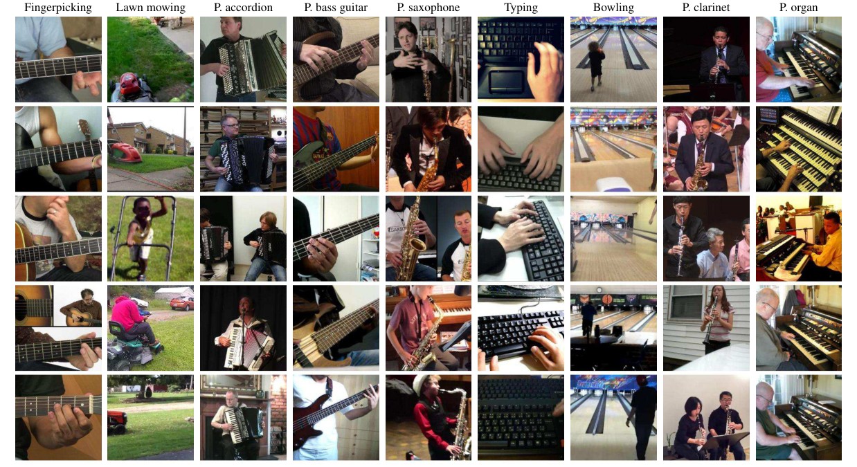
Figure 3. Learnt visual concepts. Each column shows five images that most activate a particular unit of the 512 in pool4 for the vision subnetwork. Note that these features do not take sound as input. Videos come from the Kinetics-Sounds test set and the network was trained on the Kinetics-Sounds train set. The top row shows the dominant action label for the unit (“P.” stands for “playing”).
图 3. 学到的视觉概念。每一列给出最能激活视觉子网络 pool4 中 512 个单元里某一个单元的五张图像。注意这些特征不以声音为输入。视频来自 Kinetics-Sounds 测试集,网络在 Kinetics-Sounds 训练集上训练。顶行给出该单元的主导动作标签(“P.”表示“演奏”)。
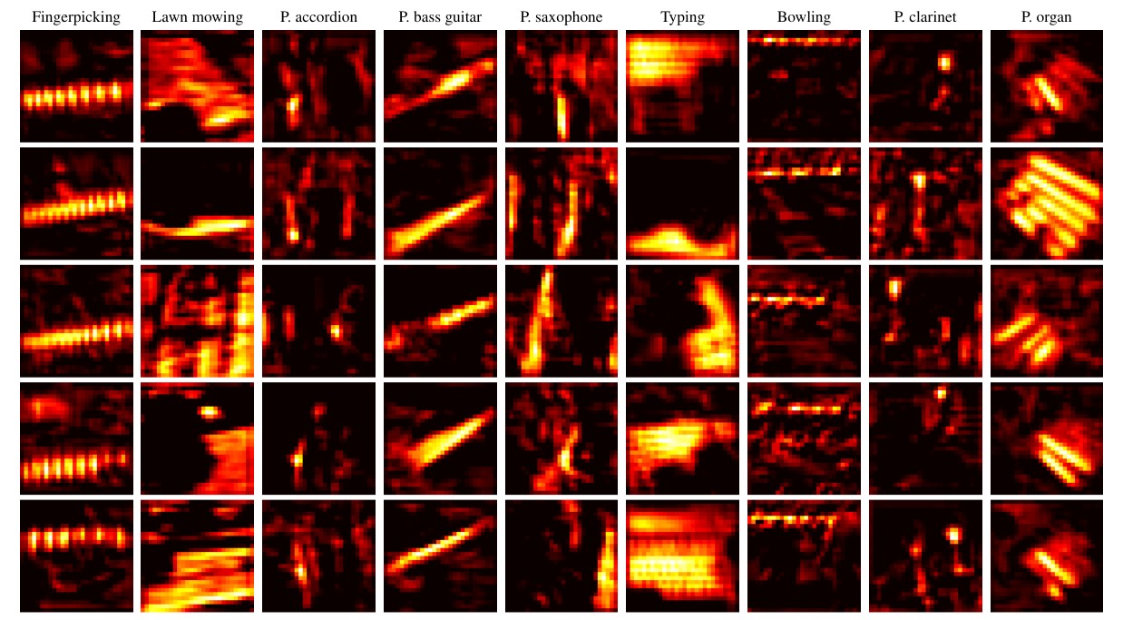
Figure 4. Visual semantic heatmap. Examples correspond to the ones in Figure 3. A semantic heatmap is obtained as a slice of activations from conv4_2 of the vision subnetwork that corresponds to the same unit from pool4 as in Figure 3, i.e. the unit that responds highly to the class in question.
图 4. 视觉语义热图。示例与图 3 中的相对应。语义热图取自视觉子网络 conv4_2 中与图 3 所用 pool4 单元相对应的那一切片激活,也就是对该类别响应很高的那个单元。
Figure 4 shows heatmaps for the images in Figure 3, obtained by simply displaying the spatial activations of the corresponding vision unit (i.e. if the component of pool4 is chosen, then the channel of conv4_2 is displayed – since the component is just the spatial max over this channel (after ReLU)). Objects are successfully detected despite significant clutter and occlusions. It is interesting to observe the type of cues that the network decides to use, e.g. the “playing clarinet” unit, instead of trying to detect the entire clarinet, seems to mostly activate on the interface between the player’s face and the clarinet.
图 4 给出图 3 中那些图像的热图,做法只是显示相应视觉单元的空间激活(也就是说,若选取 pool4 的第 个分量,就显示 conv4_2 的第 个通道——因为该分量不过是这一通道在空间上的最大值(在 ReLU 之后))。尽管有明显的杂乱和遮挡,物体仍被成功检测出来。观察网络选择使用的线索类型也很有意思,例如“演奏单簧管”单元似乎并不试图检测整支单簧管,而主要激活在演奏者面部与单簧管的交接处。
Further examples included in the extended version of this paper [2] illustrate that scene level semantic categories (as opposed to the object level categories shown here) are also learnt by the network.
本工作扩展版 [2] 中的更多例子表明,网络也学到了场景级语义类别(而不仅仅是这里展示的物体级类别)。
Audio features. Figure 5 shows what particular audio units are sensitive to. For visualization purposes, instead of showing the sound form, we display the video frame that corresponds to the sound. It can be seen that the audio subnetwork, again without any supervision, manages to learn various semantic entities, as well as perform fine-grained classification (“fingerpicking” vs “playing bass guitar”). Note that some units are naturally confused – the “tap dancing” unit also responds to “pen tapping”, while the “saxophone” unit is sometimes confused with a “trombone”. These are reasonable mistakes, especially when taking into account that the sound input is only one second in length.
音频特征。 图 5 展示特定音频单元对什么敏感。出于可视化考虑,我们不展示声波本身,而显示与该声音对应的视频帧。可以看到,音频子网络同样在没有任何监督的情况下,学会了各种语义实体,并能做细粒度分类(“fingerpicking”与“playing bass guitar”)。需要注意,有些单元会出现很自然的混淆——“踢踏舞”单元也会对“敲笔”有响应,而“萨克斯”单元有时会与“长号”混淆。这些都是合理的错误,尤其是考虑到声音输入只有一秒长。
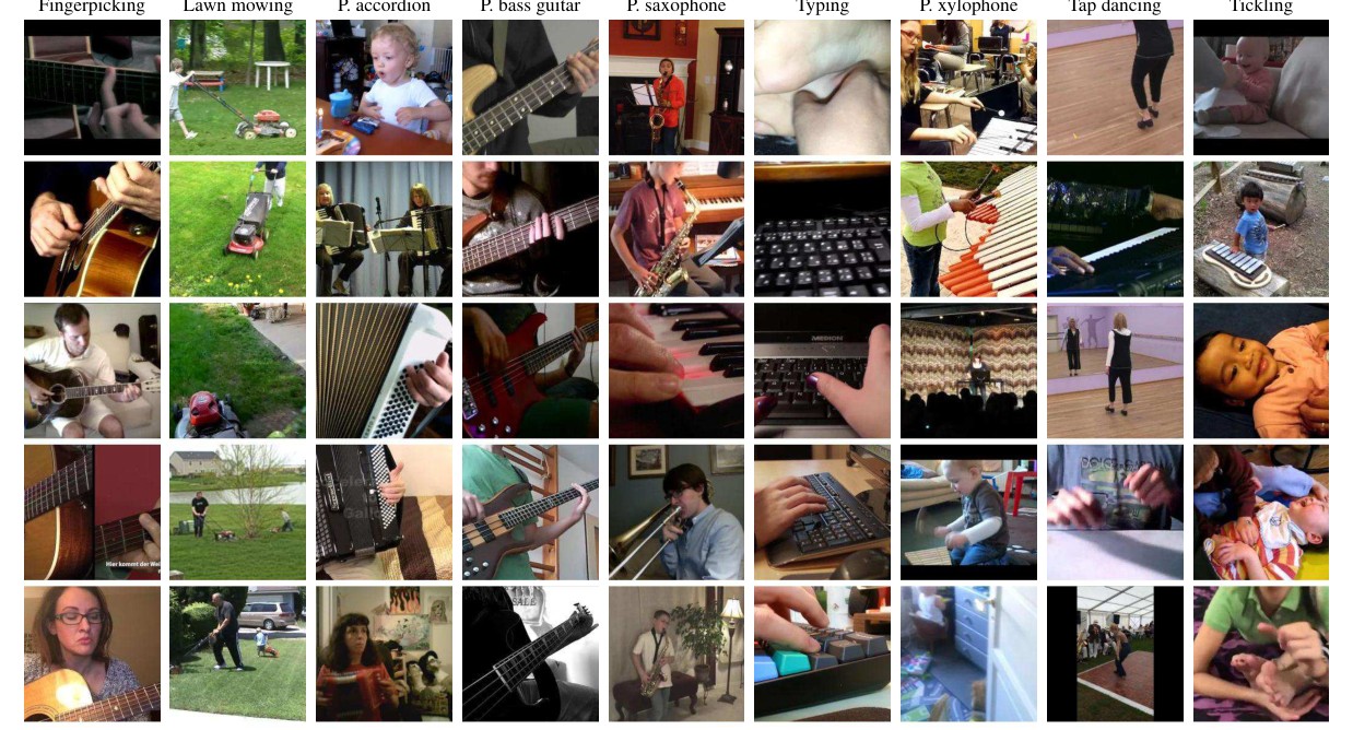
Figure 5. Learnt audio concepts. Each column shows five sounds that most activate a particular unit in pool4 of the audio subnetwork. Purely for visualization purposes, as it is hard to display sound, the frame of the video that is aligned with the sound is shown instead of the actual sound form, but we stress that no vision is used in this experiment. Videos come from the Kinetics-Sounds test set and the network was trained on the Kinetics-Sounds train set. The top row shows the dominant action label for the unit (“P.” stands for “playing”).
图 5. 学到的音频概念。每一列给出最能激活音频子网络 pool4 中某一个单元的五段声音。纯粹为了可视化——因为声音很难展示——我们显示的是与该声音对齐的视频帧,而不是实际波形,但需要强调,本实验并不使用视觉。视频来自 Kinetics-Sounds 测试集,网络在 Kinetics-Sounds 训练集上训练。顶行给出该单元的主导动作标签(“P.”表示“演奏”)。
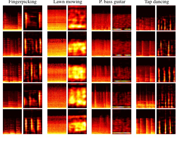
Figure 6. Audio semantic heatmaps. Each pair of columns shows a single action class (top, “P.” stands for “playing”), five log-spectrograms (left) and spectrogram semantic heatmaps (right) for the class. Horizontal and vertical axes correspond to the time and frequency dimensions, respectively. A semantic heatmap is obtained as a slice of activations of the unit from conv4_2 of the audio subnetwork which shows preference for the considered class.
图 6. 音频语义热图。每一对列给出一个动作类别(顶部,“P.”表示“演奏”),以及该类别的五张对数谱图(左)和谱图语义热图(右)。横轴和纵轴分别对应时间和频率。语义热图取自音频子网络 conv4_2 中对该类别表现出偏好的那个单元的激活切片。
Figure 6 shows spectrograms and their semantic heatmaps, illustrating that our -Net learns to detect audio events. For example, it shows clear preference for low frequencies when detecting bass guitars, attention to wide frequency range when detecting lawnmowers, and temporal ‘steps’ when detecting fingerpicking and tap dancing.
图 6 给出谱图及其语义热图,说明我们的 -Net 学会了检测音频事件。例如,检测贝斯时对低频有明显偏好,检测割草机时关注较宽的频率范围,检测指弹吉他和踢踏舞时则出现时间上的“步伐”。
Versus random features. Could the results in Figures 3 and 5 simply be obtained by chance due to examining a large number of units, as colourfully illustrated by the dead salmon experiment [4]? It is unlikely as there are only 512 units in pool4 to choose from, and many of those were found to be highly correlated with a semantic concept. Nevertheless, we repeated the same experiment with a random network (i.e. a network that has not been trained), and have failed to find such correlation. In more detail, we examined how many out of the action classes in Kinetics-Sounds have a unit in pool4 which shows high preference for the class. For the vision subnetwork the preference is determined by ranking all images by their unit activation, and retaining the top 5; if 4 out of these 5 images correspond to one class, then that class is deemed to have a high-preference for the unit (a similar procedure is carried out for the audio subnetwork using spectrograms). Our trained vision and audio networks have high-preference units for 10 and 11 out of a possible 34 action classes, respectively, compared to 1 and 1 for the random vision and audio networks. Furthermore, if the threshold for deeming a unit to be high-preference is reduced to 3, our trained vision and audio subnetworks cover 23 and 20 classes, respectively, compared to the 4 and 3 of a random network, respectively. These results confirm that our network has indeed learnt semantic features.
与随机特征对照。 图 3 和图 5 中的结果,会不会只是因为检查了大量单元而偶然得到的,就像死鲑鱼实验 [4] 所生动展示的那样?这不太可能,因为 pool4 里可供选择的单元只有 512 个,而其中许多被发现与某个语义概念高度相关。尽管如此,我们还是用一个随机网络(即未经训练的网络)重复了同一实验,并未能发现这种相关。更具体地说,我们考察 Kinetics-Sounds 中有多少动作类别在 pool4 里拥有对该类表现出高偏好的单元。对视觉子网络,偏好的判定方式是按单元激活对所有图像排序并保留前 5 张;若这 5 张里有 4 张对应同一类,则认为该类对该单元有高偏好(对音频子网络用谱图做类似手续)。我们训练后的视觉和音频网络,分别对可能的 34 个动作类别中的 10 个和 11 个拥有高偏好单元,而随机的视觉和音频网络分别只有 1 个和 1 个。此外,若把判定高偏好的阈值降到 3,训练后的视觉和音频子网络分别覆盖 23 和 20 类,而随机网络分别只有 4 和 3 类。这些结果证实,我们的网络确实学到了语义特征。
4. Discussion
4. 讨论
We have shown that the network trained for the AVC task achieves superior results on sound classification to recent methods that pre-train and fix the visual networks (one each for ImageNet and Scenes), and we conjecture that the reason for this is that the additional freedom of the visual network allows the learning to better take advantage of the opportunities offered by the variety of visual information in the video (rather than be restricted to seeing only through the eyes of the pre-trained network). Also, the visual features that emerge from the -Net are on par with the state-of-the-art among self-supervised approaches. Furthermore, it has been demonstrated that the network automatically learns, in both modalities, fine-grained distinctions such as bass versus acoustic guitar or saxophone versus clarinet.
我们已经表明,为 AVC 任务训练的网络在声音分类上优于近期那些预训练并固定视觉网络的方法(分别对应 ImageNet 和场景各一个),我们猜想原因在于视觉网络额外的自由度,使学习能更好地利用视频中多样视觉信息所提供的机会(而不是只能透过预训练网络的“眼睛”去看)。同时,-Net 产生的视觉特征也与自监督方法中的最好水平相当。此外,已经表明网络会在两个模态中自动学会细粒度区分,例如贝斯与原声吉他,或萨克斯与单簧管。
The localization visualization results are reminiscent of the classic highlighted pixels in [15], except in our case we do not just learn the few pixels that move (concurrent with the sound) but instead are able to learn extended regions corresponding to the instrument.
定位可视化的结果让人想起 [15] 中那些经典的高亮像素,只不过在我们这里,学到的不只是随声音一起移动的那几个像素,而是能够学到与乐器相对应的扩展区域。
We motivated this work by considering correlation of video and audio events. However, we believe there is additional information in concurrency of the two streams, as concurrency is stronger than correlation because the events need to be synchronised (of course, if events are concurrent then they will correlate, but not vice versa). Training for concurrency will require video (multiple frames) as input, rather than a single video frame, but it would be interesting to explore what more is gained from this stronger condition.
我们以视频和音频事件的相关性来引出这项工作。不过,我们认为两路信号的并发性中还有额外信息,因为并发比相关更强——事件需要同步(当然,若事件是并发的,它们就会相关,但反过来不一定成立)。为并发性而训练将需要以视频(多帧)而不是单帧作为输入,但探索这一更强条件还能带来什么,会很有意思。
In the future, it would be interesting to learn from the recently released large dataset of videos curated according to audio, rather than visual, events [11] and see what subtle visual semantic categories are discovered.
未来,从最近发布的、按音频而非视觉事件整理的大规模视频数据集 [11] 中学习,并看看能发现哪些细微的视觉语义类别,会很有意思。
References
参考文献
[1] P. Agrawal, J. Carreira, and J. Malik. Learning to see by moving. In Proc. ICCV, 2015.
[2] R. Arandjelović and A. Zisserman. Look, listen and learn. CoRR, abs/1705.08168, 2017.
[3] Y. Aytar, C. Vondrick, and A. Torralba. SoundNet: Learning sound representations from unlabeled video. In NIPS, 2016.
[4] C. M. Bennett, M. B. Miller, and G. L. Wolford. Neural correlates of interspecies perspective taking in the post-mortem Atlantic salmon: An argument for multiple comparisons correction. NeuroImage, 2009.
[5] A. Blum and T. Mitchell. Combining labeled and unlabeled data with co-training. In Computational learning theory, 1998.
[6] J. S. Chung and A. Zisserman. Out of time: Automated lip sync in the wild. In Workshop on Multi-view Lip-reading, ACCV, 2016.
[7] C. Doersch, A. Gupta, and A. A. Efros. Unsupervised visual representation learning by context prediction. In Proc. CVPR, 2015.
[8] J. Donahue, P. Krähenbühl, and T. Darrell. Adversarial feature learning. In Proc. ICLR, 2017.
[9] A. Dosovitskiy, J. T. Springenberg, M. Riedmiller, and T. Brox. Discriminative unsupervised feature learning with convolutional neural networks. In NIPS, 2014.
[10] A. Frome, G. S. Corrado, J. Shlens, S. Bengio, J. Dean, M. A. Ranzato, and T. Mikolov. Devise: A deep visual-semantic embedding model. In NIPS, 2013.
[11] J. F. Gemmeke, D. P. W. Ellis, D. Freedman, A. Jansen, W. Lawrence, R. C. Moore, M. Plakal, and M. Ritter. Audio Set: An ontology and human-labeled dataset for audio events. In ICASSP, 2017.
[12] D. Harwath, A. Torralba, and J. R. Glass. Unsupervised learning of spoken language with visual context. In NIPS, 2016.
[13] S. Ioffe and C. Szegedy. Batch normalization: Accelerating deep network training by reducing internal covariate shift. In Proc. ICML, 2015.
[14] W. Kay, J. Carreira, K. Simonyan, B. Zhang, C. Hillier, S. Vijayanarasimhan, F. Viola, T. Green, T. Back, P. Natsev, M. Suleyman, and A. Zisserman. The Kinetics human action video dataset. CoRR, abs/1705.06950, 2017.
[15] E. Kidron, Y. Y. Schechner, and M. Elad. Pixels that sound. In Proc. CVPR, 2005.
[16] D. P. Kingma and J. Ba. Adam: A method for stochastic optimization. In Proc. ICLR, 2015.
[17] P. Krähenbühl, C. Doersch, J. Donahue, and T. Darrell. Data-dependent initializations of convolutional neural networks. In Proc. ICLR, 2015.
[18] A. Krizhevsky, I. Sutskever, and G. E. Hinton. ImageNet classification with deep convolutional neural networks. In NIPS, pages 1106–1114, 2012.
[19] J. Lei Ba, K. Swersky, S. Fidler, and R. Salakhutdinov. Predicting deep zero-shot convolutional neural networks using textual descriptions. In Proc. ICCV, 2015.
[20] D. Li, J. Tam, and D. Toub. Auditory scene classification using machine learning techniques. IEEE AASP Challenge on Detection and Classification of Acoustic Scenes and Events, 2013.
[21] I. Misra, C. L. Zitnick, and M. Herbert. Shuffle and learn: Unsupervised learning using temporal order verification. In Proc. ECCV, 2016.
[22] M. Noroozi and P. Favaro. Unsupervised learning of visual representations by solving jigsaw puzzles. In Proc. ECCV, 2016.
[23] A. Owens, P. Isola, J. McDermott, A. Torralba, E. Adelson, and W. Freeman. Visually indicated sounds. In Proc. CVPR, 2016.
[24] A. Owens, W. Jiajun, J. McDermott, W. Freeman, and A. Torralba. Ambient sound provides supervision for visual learning. In Proc. ECCV, 2016.
[25] D. Pathak, P. Krähenbühl, J. Donahue, T. Darrell, and A. A. Efros. Context encoders: Feature learning by inpainting. In Proc. CVPR, 2016.
[26] K. J. Piczak. Environmental sound classification with convolutional neural networks. In IEEE Workshop on Machine Learning for Signal processing, 2015.
[27] K. J. Piczak. ESC: Dataset for environmental sound classification. In Proc. ACMM, 2015.
[28] A. Rakotomamonjy and G. Gasso. Histogram of gradients of time-frequency representations for audio scene classification. IEEE/ACM Transactions on Audio, Speech, and Language Processing, 2015.
[29] G. Roma, W. Nogueira, and P. Herrera. Recurrence quantification analysis features for environmental sound recognition. In IEEE Workshop on Applications of Signal Processing to Audio and Acoustics (WASPAA), 2013.
[30] O. Russakovsky, J. Deng, H. Su, J. Krause, S. Satheesh, S. Ma, S. Huang, A. Karpathy, A. Khosla, M. Bernstein, A. Berg, and F. Li. Imagenet large scale visual recognition challenge. IJCV, 2015.
[31] K. Simonyan and A. Zisserman. Very deep convolutional networks for large-scale image recognition. In Proc. ICLR, 2015.
[32] R. Socher, M. Ganjoo, C. D. Manning, and A. Ng. Zero-shot learning through cross-modal transfer. In NIPS, 2013.
[33] D. Stowell, D. Giannoulis, E. Benetos, M. Lagrange, and M. D. Plumbley. Detection and classification of acoustic scenes and events. In IEEE Transactions on Multimedia, 2015.
[34] C. Szegedy, V. Vanhoucke, S. Ioffe, J. Shlens, and Z. Wojna. Rethinking the Inception architecture for computer vision. In Proc. CVPR, 2016.
[35] X. Wang and A. Gupta. Unsupervised learning of visual representations using videos. In Proc. ICCV, 2015.
[36] R. Zhang, P. Isola, and A. A. Efros. Colorful image colorization. In Proc. ECCV, 2016.