Characterizing the Expressivity of Local Attention in Transformers
Characterizing the Expressivity of Local Attention in Transformers
Jiaoda Li Ryan Cotterell Affiliation: { jiaoda.li , ryan.cotterell }@inf.ethz.ch Affiliation:
Abstract
摘要
The transformer is the most popular neural architecture for language modeling. The cornerstone of the transformer is its global attention mechanism, which lets the model aggregate information from all preceding tokens before generating the next token. One common variant of attention is called local attention, which restricts each token to aggregating information from a bounded window of predecessors, reducing the quadratic cost of global attention to linear. Although this restriction is usually motivated by efficiency, it has also been found to improve model quality, a phenomenon that has so far lacked a satisfactory explanation. We provide a formal account of this phenomenon in terms of recognizer expressivity. It has been shown that fixed-precision transformers with global attention correspond to a fragment of linear temporal logic containing a single past operator. We additionally prove that adding local attention introduces a second temporal operator, strictly enlarging the class of recognizable regular languages. Moreover, global and local attention are expressively complementary: neither subsumes the other, and combining them yields the richest fragment. Experiments on formal language recognition and natural language modeling corroborate the theory, showing that hybrid global–local transformers outperform their global-only counterparts.
Transformer 是目前最常用的语言建模神经结构。它的核心是全局注意力机制:在生成下一个词元之前,模型可以从此前全部词元中聚合信息。注意力的一种常见变体叫做局部注意力,它把每个词元的聚合范围限制在前面一个有界窗口里,从而把全局注意力的平方代价降为线性。这一限制通常是出于效率考虑,却也常被发现能够提高模型质量,而这一现象迄今缺少令人满意的解释。我们从识别器表达力的角度给出形式说明。已有结果表明,带全局注意力的固定精度 Transformer 对应线性时序逻辑中只含一个过去算子的片段。我们进一步证明,加入局部注意力会引入第二个时序算子,从而严格扩大可识别的正则语言类。此外,全局注意力与局部注意力在表达力上是互补的:二者互不包含,合在一起得到最丰富的片段。形式语言识别与自然语言建模上的实验与理论相符,表明全局–局部混合的 Transformer 优于只使用全局注意力的对照模型。
1 Introduction
1 引言
The transformer (Vaswani et al., 2017) is the dominant neural architecture in modern language modeling (Radford et al., 2018; Radford et al., 2019; Brown et al., 2020; OpenAI, 2023). At its core lies the attention mechanism (Schmidhuber, 1992; Bahdanau et al., 2015), which allows the model to aggregate information from all previously generated tokens before generating the next one. Local attention (Luong et al., 2015; Child et al., 2019; Beltagy et al., 2020; Zaheer et al., 2020) is a popular attention variant that restricts the model to aggregating over a fixed-size window of preceding tokens.
Transformer(Vaswani et al., 2017)是现代语言建模中的主流神经结构(Radford et al., 2018; Radford et al., 2019; Brown et al., 2020; OpenAI, 2023)。其核心是注意力机制(Schmidhuber, 1992; Bahdanau et al., 2015),使模型在生成下一个词元之前,能够从已经生成的全部词元中聚合信息。局部注意力(Luong et al., 2015; Child et al., 2019; Beltagy et al., 2020; Zaheer et al., 2020)是一种常用变体,它把聚合范围限制在前面一个固定大小的窗口里。
Local attention is typically motivated by efficiency. Standard global attention aggregates over all previous positions, incurring quadratic cost in sequence length; local attention reduces this to linear. At first glance, restricting the range of tokens that a transformer can attend to appears to be a strict weakening—a trade-off of expressivity for speed. Surprisingly, however, local attention has been repeatedly observed to yield empirical improvements, both in machine translation (Luong et al., 2015) and in language modeling (Child et al., 2019; Beltagy et al., 2020; Zaheer et al., 2020)—even when computational budgets are held constant.
局部注意力通常是出于效率提出的。标准的全局注意力要对所有先前位置做聚合,代价随序列长度呈平方增长;局部注意力把它降为线性。乍看之下,限制 Transformer 能够关注的词元范围,似乎是表达力上的严格削弱——用表达力换速度。然而出人意料的是,局部注意力一再被观察到带来经验上的改进,无论是在机器翻译(Luong et al., 2015)还是语言建模(Child et al., 2019; Beltagy et al., 2020; Zaheer et al., 2020)中——即便在算力预算保持不变的情况下也是如此。
We resolve this puzzle by analyzing which formal languages different attention patterns can recognize, a standard lens in the formal study of neural models (Delétang et al., 2023; Butoi et al., 2025). This lens also has practical relevance: modern language models (OpenAI, 2023; DeepSeek-AI, 2025; Team et al., 2025) are routinely used to perform computation via prompting (Wei et al., 2022; Li et al., 2024; Merrill and Sabharwal, 2024). In this vein, Li and Cotterell (2025) show that fixed-precision transformer language models with global attention correspond exactly to the fragment of linear temporal logic with a single past operator. Expanding their work, we prove that adding local attention introduces a new temporal operator, enabling the recognition of a strictly larger class of regular languages. These include the locally testable languages, a family closely connected to -gram models and extensively studied in formal language theory (McNaughton and Papert, 1971, Ch. 2). Crucially, local attention is complementary rather than a drop-in replacement for global attention: with purely local attention, the computation depends only on a fixed-length suffix of the input, collapsing expressivity to the smaller class of definite languages (Kleene, 1956, §5).
我们通过分析不同注意力模式能够识别哪些形式语言来解开这一困惑,这是形式地研究神经模型时的标准视角(Delétang et al., 2023; Butoi et al., 2025)。这一视角也有直接的应用意义:现代语言模型(OpenAI, 2023; DeepSeek-AI, 2025; Team et al., 2025)常常被通过提示来执行计算(Wei et al., 2022; Li et al., 2024; Merrill and Sabharwal, 2024)。沿这一方向,Li and Cotterell (2025) 证明,带全局注意力的固定精度 Transformer 语言模型恰好对应线性时序逻辑中只含一个过去算子的片段。在他们工作的基础上,我们证明加入局部注意力会引入一个新的时序算子,从而能够识别严格更大的一类正则语言。其中包括局部可检验语言,这一族与 -gram 模型关系密切,并在形式语言理论中得到过充分研究(McNaughton and Papert, 1971, Ch. 2)。关键在于,局部注意力是对全局注意力的补充,而不是可以随手替换的替代品:若只使用纯局部注意力,计算只依赖于输入一个固定长度的后缀,表达力便塌缩到更小的定语言类(Kleene, 1956, §5)。
Empirically, we test these predictions on formal language recognition with length generalization. We compare transformers with (i) global attention, (ii) local attention, and (iii) a hybrid that mixes global and local attention. The results align with the theory: hybrid models recognize strictly more languages than either extreme and generalize more reliably to longer sequences. Varying local attention’s window size further shows that a window of size one is consistently the strongest choice in the local-attention family, both for purely local models and for hybrid models. Finally, we evaluate models equipped with two popular positional encodings—sinusoidal (SiPE) and rotary (RoPE)—and find that neither compensates for the absence of local attention. We further show that these findings extend to natural language: on WikiText-2, hybrid attention with a window of size one consistently achieves the lowest perplexity across positional encodings.
在经验上,我们用带长度泛化的形式语言识别来检验这些预测。我们比较三类 Transformer:(i)全局注意力,(ii)局部注意力,以及(iii)把全局与局部混合起来的模型。结果与理论一致:混合模型能识别的语言严格多于任一极端,并且能更可靠地泛化到更长的串。进一步改变局部注意力的窗口大小后可以看到,窗口取一在局部注意力这一族里始终是最强的选择,无论是纯局部模型还是混合模型都是如此。最后,我们评估配备两种常用位置编码——正弦(SiPE)与旋转(RoPE)——的模型,发现二者都补不上缺少局部注意力所留下的缺口。我们还表明这些发现可以延伸到自然语言:在 WikiText-2 上,窗口取一的混合注意力在各种位置编码下都取得最低的困惑度。
2 Linear Temporal Logic
2 线性时序逻辑
In this section, we introduce linear temporal logic, the main tool we use to characterize the expressive power of transformers under different types of attention. We examine the fragments relevant to our analysis, prove the separations between them, and connect them to classical characterizations from algebraic formal language theory.
本节介绍线性时序逻辑,这是我们刻画不同注意力类型下 Transformer 表达力的主要工具。我们考察与分析相关的片段,证明它们之间的分离,并把它们与代数形式语言理论中的经典刻画联系起来。
2.1 Preliminaries
2.1 预备知识
We now introduce linear temporal logic (Kamp, 1968; Pnueli, 1977, LTL;), which has become a popular tool in the analysis of transformers (Yang et al., 2024; Yang et al., 2026; Li and Cotterell, 2025).
下面介绍线性时序逻辑(Kamp, 1968; Pnueli, 1977, LTL;),它已成为分析 Transformer 的常用工具(Yang et al., 2024; Yang et al., 2026; Li and Cotterell, 2025)。
Tokens, Strings and Languages.
An alphabet is a finite, non-empty set of tokens. Fix an alphabet {{\color[rgb]{0.0781,0.2148,0.5313}\Sigma}}. A string over {{\color[rgb]{0.0781,0.2148,0.5313}\Sigma}} is a finite sequence of tokens drawn from {{\color[rgb]{0.0781,0.2148,0.5313}\Sigma}}. The length of a string {{\color[rgb]{0.0781,0.2148,0.5313}\textbf{{w}}}}={\color[rgb]{0.0781,0.2148,0.5313}\texttt{w}}_{1}\cdots{\color[rgb]{0.0781,0.2148,0.5313}\texttt{w}}_{N}, denoted |{{\color[rgb]{0.0781,0.2148,0.5313}\textbf{{w}}}}|=N, is the number of tokens it contains. We write {{{{\color[rgb]{0.0781,0.2148,0.5313}\Sigma}}^{*}}} for the set of all strings over {{\color[rgb]{0.0781,0.2148,0.5313}\Sigma}}, and call any subset {{\color[rgb]{0.0781,0.2148,0.5313}L}}\subseteq{{{{\color[rgb]{0.0781,0.2148,0.5313}\Sigma}}^{*}}} a language.
词元、字符串与语言。
字母表是一个有限且非空的词元集合。固定一个字母表 {{\color[rgb]{0.0781,0.2148,0.5313}\Sigma}}。其上的字符串是由 {{\color[rgb]{0.0781,0.2148,0.5313}\Sigma}} 中词元构成的有限序列。字符串 {{\color[rgb]{0.0781,0.2148,0.5313}\textbf{{w}}}}={\color[rgb]{0.0781,0.2148,0.5313}\texttt{w}}_{1}\cdots{\color[rgb]{0.0781,0.2148,0.5313}\texttt{w}}_{N} 的长度记作 |{{\color[rgb]{0.0781,0.2148,0.5313}\textbf{{w}}}}|=N,即它所含词元的个数。我们用 {{{{\color[rgb]{0.0781,0.2148,0.5313}\Sigma}}^{*}}} 表示 {{\color[rgb]{0.0781,0.2148,0.5313}\Sigma}} 上全部字符串的集合,并把任意子集 {{\color[rgb]{0.0781,0.2148,0.5313}L}}\subseteq{{{{\color[rgb]{0.0781,0.2148,0.5313}\Sigma}}^{*}}} 称为一个语言。
Linear Temporal Logic.
The syntax and semantics of linear temporal logic ({\color[rgb]{0.4297,0.1172,0.2148}\textup{{LTL}}}[{\color[rgb]{0,0.4297,0.2539}\mathrel{\textup{{P}}}},{\color[rgb]{0,0.4297,0.2539}\mathrel{\textup{{Y}}}},{\color[rgb]{0,0.4297,0.2539}\mathrel{\textup{{S}}}},{\color[rgb]{0,0.4297,0.2539}\mathrel{\textup{{U}}}}]) as well as the definition of operator depth are recalled in Appendix A. We also give a definition of what it means for a formula in LTL to define a language; see § A.3. Given a formula {\color[rgb]{0.6875,0.2734,0.1172}\psi}, we write {{\color[rgb]{0.0781,0.2148,0.5313}\mathbb{L}}}({\color[rgb]{0.6875,0.2734,0.1172}\psi}) for the set of all strings satisfying {\color[rgb]{0.6875,0.2734,0.1172}\psi}.
线性时序逻辑。
线性时序逻辑({\color[rgb]{0.4297,0.1172,0.2148}\textup{{LTL}}}[{\color[rgb]{0,0.4297,0.2539}\mathrel{\textup{{P}}}},{\color[rgb]{0,0.4297,0.2539}\mathrel{\textup{{Y}}}},{\color[rgb]{0,0.4297,0.2539}\mathrel{\textup{{S}}}},{\color[rgb]{0,0.4297,0.2539}\mathrel{\textup{{U}}}}])的语法与语义,以及算子深度的定义,回顾于附录 A。我们也给出 LTL 公式定义一个语言是什么意思;见 § A.3。给定公式 {\color[rgb]{0.6875,0.2734,0.1172}\psi},我们把满足 {\color[rgb]{0.6875,0.2734,0.1172}\psi} 的全部字符串之集记作 {{\color[rgb]{0.0781,0.2148,0.5313}\mathbb{L}}}({\color[rgb]{0.6875,0.2734,0.1172}\psi})。
Fragments of {\color[rgb]{0.4297,0.1172,0.2148}\textup{{LTL}}}[{\color[rgb]{0,0.4297,0.2539}\mathrel{\textup{{P}}}},{\color[rgb]{0,0.4297,0.2539}\mathrel{\textup{{Y}}}},{\color[rgb]{0,0.4297,0.2539}\mathrel{\textup{{S}}}},{\color[rgb]{0,0.4297,0.2539}\mathrel{\textup{{U}}}}].
For a set of temporal operators {\color[rgb]{0,0.4297,0.2539}\mathcal{O}}\subseteq\{{\color[rgb]{0,0.4297,0.2539}\mathrel{\textup{{P}}}},{\color[rgb]{0,0.4297,0.2539}\mathrel{\textup{{Y}}}},{\color[rgb]{0,0.4297,0.2539}\mathrel{\textup{{S}}}},{\color[rgb]{0,0.4297,0.2539}\mathrel{\textup{{U}}}}\}, we write {\color[rgb]{0.4297,0.1172,0.2148}\textup{{LTL}}}[{\color[rgb]{0,0.4297,0.2539}\mathcal{O}}] for the corresponding fragment in which only operators from {\color[rgb]{0,0.4297,0.2539}\mathcal{O}} are allowed.
{\color[rgb]{0.4297,0.1172,0.2148}\textup{{LTL}}}[{\color[rgb]{0,0.4297,0.2539}\mathrel{\textup{{P}}}},{\color[rgb]{0,0.4297,0.2539}\mathrel{\textup{{Y}}}},{\color[rgb]{0,0.4297,0.2539}\mathrel{\textup{{S}}}},{\color[rgb]{0,0.4297,0.2539}\mathrel{\textup{{U}}}}] 的片段。
对时序算子集合 {\color[rgb]{0,0.4297,0.2539}\mathcal{O}}\subseteq\{{\color[rgb]{0,0.4297,0.2539}\mathrel{\textup{{P}}}},{\color[rgb]{0,0.4297,0.2539}\mathrel{\textup{{Y}}}},{\color[rgb]{0,0.4297,0.2539}\mathrel{\textup{{S}}}},{\color[rgb]{0,0.4297,0.2539}\mathrel{\textup{{U}}}}\},我们把只允许使用 {\color[rgb]{0,0.4297,0.2539}\mathcal{O}} 中算子的相应片段记作 {\color[rgb]{0.4297,0.1172,0.2148}\textup{{LTL}}}[{\color[rgb]{0,0.4297,0.2539}\mathcal{O}}]。
Definition 2.1.
Let {\color[rgb]{0,0.4297,0.2539}\mathcal{O}}\subseteq\{{\color[rgb]{0,0.4297,0.2539}\mathrel{\textup{{P}}}},{\color[rgb]{0,0.4297,0.2539}\mathrel{\textup{{Y}}}},{\color[rgb]{0,0.4297,0.2539}\mathrel{\textup{{S}}}},{\color[rgb]{0,0.4297,0.2539}\mathrel{\textup{{U}}}}\} be a set of temporal operators. A language {{\color[rgb]{0.0781,0.2148,0.5313}L}} is definable by {\color[rgb]{0.4297,0.1172,0.2148}\textup{{LTL}}}[{\color[rgb]{0,0.4297,0.2539}\mathcal{O}}] if there exists a formula {\color[rgb]{0.6875,0.2734,0.1172}\psi} in {\color[rgb]{0.4297,0.1172,0.2148}\textup{{LTL}}}[{\color[rgb]{0,0.4297,0.2539}\mathcal{O}}] such that {{\color[rgb]{0.0781,0.2148,0.5313}\mathbb{L}}}({\color[rgb]{0.6875,0.2734,0.1172}\psi})={{\color[rgb]{0.0781,0.2148,0.5313}L}}.
定义 2.1。
设 {\color[rgb]{0,0.4297,0.2539}\mathcal{O}}\subseteq\{{\color[rgb]{0,0.4297,0.2539}\mathrel{\textup{{P}}}},{\color[rgb]{0,0.4297,0.2539}\mathrel{\textup{{Y}}}},{\color[rgb]{0,0.4297,0.2539}\mathrel{\textup{{S}}}},{\color[rgb]{0,0.4297,0.2539}\mathrel{\textup{{U}}}}\} 为时序算子的集合。若存在 {\color[rgb]{0.4297,0.1172,0.2148}\textup{{LTL}}}[{\color[rgb]{0,0.4297,0.2539}\mathcal{O}}] 中的公式 {\color[rgb]{0.6875,0.2734,0.1172}\psi},使得 {{\color[rgb]{0.0781,0.2148,0.5313}\mathbb{L}}}({\color[rgb]{0.6875,0.2734,0.1172}\psi})={{\color[rgb]{0.0781,0.2148,0.5313}L}},则称语言 {{\color[rgb]{0.0781,0.2148,0.5313}L}} 可被 {\color[rgb]{0.4297,0.1172,0.2148}\textup{{LTL}}}[{\color[rgb]{0,0.4297,0.2539}\mathcal{O}}] 定义。
Gabbay et al. (1980) show that every language definable by {\color[rgb]{0.4297,0.1172,0.2148}\textup{{LTL}}}[{\color[rgb]{0,0.4297,0.2539}\mathrel{\textup{{P}}}},{\color[rgb]{0,0.4297,0.2539}\mathrel{\textup{{Y}}}},{\color[rgb]{0,0.4297,0.2539}\mathrel{\textup{{S}}}},{\color[rgb]{0,0.4297,0.2539}\mathrel{\textup{{U}}}}] is also definable by both {\color[rgb]{0.4297,0.1172,0.2148}\textup{{LTL}}}[{\color[rgb]{0,0.4297,0.2539}\mathrel{\textup{{S}}}}] and {\color[rgb]{0.4297,0.1172,0.2148}\textup{{LTL}}}[{\color[rgb]{0,0.4297,0.2539}\mathrel{\textup{{U}}}}]; in the paper, we write {\color[rgb]{0.4297,0.1172,0.2148}\textup{{LTL}}}[{\color[rgb]{0,0.4297,0.2539}\mathrel{\textup{{S}}}}] for full linear temporal logic. The fragments {\color[rgb]{0.4297,0.1172,0.2148}\textup{{LTL}}}\left[{\color[rgb]{0,0.4297,0.2539}\mathrel{\textup{{P}}}}\right] and {\color[rgb]{0.4297,0.1172,0.2148}\textup{{LTL}}}\left[{\color[rgb]{0,0.4297,0.2539}\mathrel{\textup{{Y}}}}\right] are strictly less expressive, i.e., there exist languages definable by {\color[rgb]{0.4297,0.1172,0.2148}\textup{{LTL}}}[{\color[rgb]{0,0.4297,0.2539}\mathrel{\textup{{S}}}}] that are not definable by either {\color[rgb]{0.4297,0.1172,0.2148}\textup{{LTL}}}\left[{\color[rgb]{0,0.4297,0.2539}\mathrel{\textup{{P}}}}\right] or {\color[rgb]{0.4297,0.1172,0.2148}\textup{{LTL}}}\left[{\color[rgb]{0,0.4297,0.2539}\mathrel{\textup{{Y}}}}\right].
Gabbay et al. (1980) 表明,凡是能被 {\color[rgb]{0.4297,0.1172,0.2148}\textup{{LTL}}}[{\color[rgb]{0,0.4297,0.2539}\mathrel{\textup{{P}}}},{\color[rgb]{0,0.4297,0.2539}\mathrel{\textup{{Y}}}},{\color[rgb]{0,0.4297,0.2539}\mathrel{\textup{{S}}}},{\color[rgb]{0,0.4297,0.2539}\mathrel{\textup{{U}}}}] 定义的语言,也都能被 {\color[rgb]{0.4297,0.1172,0.2148}\textup{{LTL}}}[{\color[rgb]{0,0.4297,0.2539}\mathrel{\textup{{S}}}}] 和 {\color[rgb]{0.4297,0.1172,0.2148}\textup{{LTL}}}[{\color[rgb]{0,0.4297,0.2539}\mathrel{\textup{{U}}}}] 定义;文中我们用 {\color[rgb]{0.4297,0.1172,0.2148}\textup{{LTL}}}[{\color[rgb]{0,0.4297,0.2539}\mathrel{\textup{{S}}}}] 指称完整的线性时序逻辑。片段 {\color[rgb]{0.4297,0.1172,0.2148}\textup{{LTL}}}\left[{\color[rgb]{0,0.4297,0.2539}\mathrel{\textup{{P}}}}\right] 与 {\color[rgb]{0.4297,0.1172,0.2148}\textup{{LTL}}}\left[{\color[rgb]{0,0.4297,0.2539}\mathrel{\textup{{Y}}}}\right] 的表达力严格较弱,也就是说,存在能被 {\color[rgb]{0.4297,0.1172,0.2148}\textup{{LTL}}}[{\color[rgb]{0,0.4297,0.2539}\mathrel{\textup{{S}}}}] 定义、却不能被 {\color[rgb]{0.4297,0.1172,0.2148}\textup{{LTL}}}\left[{\color[rgb]{0,0.4297,0.2539}\mathrel{\textup{{P}}}}\right] 或 {\color[rgb]{0.4297,0.1172,0.2148}\textup{{LTL}}}\left[{\color[rgb]{0,0.4297,0.2539}\mathrel{\textup{{Y}}}}\right] 定义的语言。
2.2 Characterizing {\color[rgb]{0.4297,0.1172,0.2148}\textup{{LTL}}}\left[{\color[rgb]{0,0.4297,0.2539}\mathrel{\textup{{Y}}}}\right]
2.2 刻画 {\color[rgb]{0.4297,0.1172,0.2148}\textup{{LTL}}}\left[{\color[rgb]{0,0.4297,0.2539}\mathrel{\textup{{Y}}}}\right]
We first characterize the expressive power of {\color[rgb]{0.4297,0.1172,0.2148}\textup{{LTL}}}\left[{\color[rgb]{0,0.4297,0.2539}\mathrel{\textup{{Y}}}}\right] by relating it to a classical class of regular languages. Because formulas in {\color[rgb]{0.4297,0.1172,0.2148}\textup{{LTL}}}\left[{\color[rgb]{0,0.4297,0.2539}\mathrel{\textup{{Y}}}}\right] can only look back a bounded number of steps, we show they naturally correspond to languages determined by a bounded suffix—the definite languages.
我们首先把 {\color[rgb]{0.4297,0.1172,0.2148}\textup{{LTL}}}\left[{\color[rgb]{0,0.4297,0.2539}\mathrel{\textup{{Y}}}}\right] 的表达力与一类经典的正则语言联系起来。由于 {\color[rgb]{0.4297,0.1172,0.2148}\textup{{LTL}}}\left[{\color[rgb]{0,0.4297,0.2539}\mathrel{\textup{{Y}}}}\right] 中的公式只能回看有界步数,我们证明它们自然对应由有界后缀所决定的语言——即定语言。
For a string w of length and an integer , an -factor of w is any contiguous substring of w of length . The -prefix of w is its initial substring of length , and the -suffix of w is its final substring of length . We write {\mathbb{I}}_{m}({{\color[rgb]{0.0781,0.2148,0.5313}\textbf{{w}}}}) for the set of all -factors of w, and {P}_{m}({{\color[rgb]{0.0781,0.2148,0.5313}\textbf{{w}}}}) and {S}_{m}({{\color[rgb]{0.0781,0.2148,0.5313}\textbf{{w}}}}) for the -prefix and -suffix of w, respectively. If m>|{{\color[rgb]{0.0781,0.2148,0.5313}\textbf{{w}}}}|, we set {P}_{m}({{\color[rgb]{0.0781,0.2148,0.5313}\textbf{{w}}}})={S}_{m}({{\color[rgb]{0.0781,0.2148,0.5313}\textbf{{w}}}})={{\color[rgb]{0.0781,0.2148,0.5313}\textbf{{w}}}}. Formally, a language {{\color[rgb]{0.0781,0.2148,0.5313}L}}\subseteq{{{{\color[rgb]{0.0781,0.2148,0.5313}\Sigma}}^{*}}} is -definite, for some , if {{\color[rgb]{0.0781,0.2148,0.5313}L}} is a Boolean combination of languages of the form \left\{{{\color[rgb]{0.0781,0.2148,0.5313}\textbf{{w}}}}\in{{{{\color[rgb]{0.0781,0.2148,0.5313}\Sigma}}^{*}}}\mid{S}_{m}({{\color[rgb]{0.0781,0.2148,0.5313}\textbf{{w}}}})={{\color[rgb]{0.0781,0.2148,0.5313}\textbf{{u}}}}\right\}. A language is definite if it is -definite for some .
对长度为 的字符串 w 以及整数 ,w 的一个 -因子是 w 中任意长度为 的连续子串。w 的 -前缀是其长度为 的起始子串,-后缀则是其长度为 的末尾子串。我们把 w 的全部 -因子之集记作 {\mathbb{I}}_{m}({{\color[rgb]{0.0781,0.2148,0.5313}\textbf{{w}}}}),并把 -前缀与 -后缀分别记作 {P}_{m}({{\color[rgb]{0.0781,0.2148,0.5313}\textbf{{w}}}}) 和 {S}_{m}({{\color[rgb]{0.0781,0.2148,0.5313}\textbf{{w}}}})。若 m>|{{\color[rgb]{0.0781,0.2148,0.5313}\textbf{{w}}}}|,则令 {P}_{m}({{\color[rgb]{0.0781,0.2148,0.5313}\textbf{{w}}}})={S}_{m}({{\color[rgb]{0.0781,0.2148,0.5313}\textbf{{w}}}})={{\color[rgb]{0.0781,0.2148,0.5313}\textbf{{w}}}}。形式地说,对某个 ,语言 {{\color[rgb]{0.0781,0.2148,0.5313}L}}\subseteq{{{{\color[rgb]{0.0781,0.2148,0.5313}\Sigma}}^{*}}} 是 -定的,若 {{\color[rgb]{0.0781,0.2148,0.5313}L}} 是形如 \left\{{{\color[rgb]{0.0781,0.2148,0.5313}\textbf{{w}}}}\in{{{{\color[rgb]{0.0781,0.2148,0.5313}\Sigma}}^{*}}}\mid{S}_{m}({{\color[rgb]{0.0781,0.2148,0.5313}\textbf{{w}}}})={{\color[rgb]{0.0781,0.2148,0.5313}\textbf{{u}}}}\right\} 的语言的布尔组合。若存在某个 使语言为 -定的,则称它是定语言。
We next relate {\color[rgb]{0.4297,0.1172,0.2148}\textup{{LTL}}}\left[{\color[rgb]{0,0.4297,0.2539}\mathrel{\textup{{Y}}}}\right] to definite languages, for which we also provide algebraic and automata-theoretic characterizations. The relevant background, including definitions of the syntactic semigroups and deterministic finite automata (DFAs), are recalled in Appendix B.
接下来我们把 {\color[rgb]{0.4297,0.1172,0.2148}\textup{{LTL}}}\left[{\color[rgb]{0,0.4297,0.2539}\mathrel{\textup{{Y}}}}\right] 与定语言联系起来,并为后者给出代数与自动机理论方面的刻画。相关背景,包括句法半群与确定有限自动机(DFA)的定义,回顾于附录 B。
Theorem 2.2.
Let ${{\color[rgb]{0.0781,0.2148,0.5313}L}}\subseteq{{{{\color[rgb]{0.0781,0.2148,0.5313}\Sigma}}^{}}}{\color[rgb]{0.5586,0.4023,0.0742}\mathbb{S}}{{\color[rgb]{0.5586,0.4023,0.0742}\mathcal{A}}}{{\color[rgb]{0.0781,0.2148,0.5313}L}}$. The following are equivalent:*
定理 2.2。
设 ${{\color[rgb]{0.0781,0.2148,0.5313}L}}\subseteq{{{{\color[rgb]{0.0781,0.2148,0.5313}\Sigma}}^{}}}{\color[rgb]{0.5586,0.4023,0.0742}\mathbb{S}}{{\color[rgb]{0.5586,0.4023,0.0742}\mathcal{A}}}{{\color[rgb]{0.0781,0.2148,0.5313}L}}$ 的最小 DFA。下列诸款等价:*
- {{\color[rgb]{0.0781,0.2148,0.5313}L}}is definable in{\color[rgb]{0.4297,0.1172,0.2148}\textup{{LTL}}}\left[{\color[rgb]{0,0.4297,0.2539}\mathrel{\textup{{Y}}}}\right];
- {{\color[rgb]{0.0781,0.2148,0.5313}L}} 可在 {\color[rgb]{0.4297,0.1172,0.2148}\textup{{LTL}}}\left[{\color[rgb]{0,0.4297,0.2539}\mathrel{\textup{{Y}}}}\right] 中定义;
- {{\color[rgb]{0.0781,0.2148,0.5313}L}}is definite;
- {{\color[rgb]{0.0781,0.2148,0.5313}L}} 是定语言;
- every idempotent{e}\in{\color[rgb]{0.5586,0.4023,0.0742}\mathbb{S}}is a right zero, i.e., for alls\in{\color[rgb]{0.5586,0.4023,0.0742}\mathbb{S}},;
- 每个幂等元 {e}\in{\color[rgb]{0.5586,0.4023,0.0742}\mathbb{S}} 都是右零元,即对所有 s\in{\color[rgb]{0.5586,0.4023,0.0742}\mathbb{S}},有 ;
- every transformation induced by a non-empty string is non-permutational.
- 每个由非空字符串诱导的变换都是非置换的。
Proof.
See § C.1. ∎
证明。
见 § C.1。∎
2.3 {\color[rgb]{0.4297,0.1172,0.2148}\textup{{LTL}}}\left[{\color[rgb]{0,0.4297,0.2539}\mathrel{\textup{{P}}}}\right] and {\color[rgb]{0.4297,0.1172,0.2148}\textup{{LTL}}}\left[{\color[rgb]{0,0.4297,0.2539}\mathrel{\textup{{Y}}}}\right] are Incomparable
2.3 {\color[rgb]{0.4297,0.1172,0.2148}\textup{{LTL}}}\left[{\color[rgb]{0,0.4297,0.2539}\mathrel{\textup{{P}}}}\right] 与 {\color[rgb]{0.4297,0.1172,0.2148}\textup{{LTL}}}\left[{\color[rgb]{0,0.4297,0.2539}\mathrel{\textup{{Y}}}}\right] 不可比
Li and Cotterell (2025) give a rich characterization of {\color[rgb]{0.4297,0.1172,0.2148}\textup{{LTL}}}\left[{\color[rgb]{0,0.4297,0.2539}\mathrel{\textup{{P}}}}\right]. Building on this and Section 2.2, we now relate {\color[rgb]{0.4297,0.1172,0.2148}\textup{{LTL}}}\left[{\color[rgb]{0,0.4297,0.2539}\mathrel{\textup{{P}}}}\right] and {\color[rgb]{0.4297,0.1172,0.2148}\textup{{LTL}}}\left[{\color[rgb]{0,0.4297,0.2539}\mathrel{\textup{{Y}}}}\right]. However, we first discuss what it means to compare two sets of operators for linear temporal logic. Fix {\color[rgb]{0,0.4297,0.2539}\mathcal{O}}_{1},{\color[rgb]{0,0.4297,0.2539}\mathcal{O}}_{2}\subseteq\{{\color[rgb]{0,0.4297,0.2539}\mathrel{\textup{{P}}}},{\color[rgb]{0,0.4297,0.2539}\mathrel{\textup{{Y}}}},{\color[rgb]{0,0.4297,0.2539}\mathrel{\textup{{S}}}},{\color[rgb]{0,0.4297,0.2539}\mathrel{\textup{{U}}}}\}. We say {\color[rgb]{0.4297,0.1172,0.2148}\textup{{LTL}}}[{\color[rgb]{0,0.4297,0.2539}\mathcal{O}}_{1}] is more expressive than {\color[rgb]{0.4297,0.1172,0.2148}\textup{{LTL}}}[{\color[rgb]{0,0.4297,0.2539}\mathcal{O}}_{2}], written in symbols {\color[rgb]{0.4297,0.1172,0.2148}\textup{{LTL}}}[{\color[rgb]{0,0.4297,0.2539}\mathcal{O}}_{2}]\subseteq{\color[rgb]{0.4297,0.1172,0.2148}\textup{{LTL}}}[{\color[rgb]{0,0.4297,0.2539}\mathcal{O}}_{1}], if every language definable in {\color[rgb]{0.4297,0.1172,0.2148}\textup{{LTL}}}[{\color[rgb]{0,0.4297,0.2539}\mathcal{O}}_{2}] is also definable in {\color[rgb]{0.4297,0.1172,0.2148}\textup{{LTL}}}[{\color[rgb]{0,0.4297,0.2539}\mathcal{O}}_{1}]. We say {\color[rgb]{0.4297,0.1172,0.2148}\textup{{LTL}}}[{\color[rgb]{0,0.4297,0.2539}\mathcal{O}}_{1}] is strictly more expressive than {\color[rgb]{0.4297,0.1172,0.2148}\textup{{LTL}}}[{\color[rgb]{0,0.4297,0.2539}\mathcal{O}}_{2}], written in symbols as {\color[rgb]{0.4297,0.1172,0.2148}\textup{{LTL}}}[{\color[rgb]{0,0.4297,0.2539}\mathcal{O}}_{2}]\subset{\color[rgb]{0.4297,0.1172,0.2148}\textup{{LTL}}}[{\color[rgb]{0,0.4297,0.2539}\mathcal{O}}_{1}], if {\color[rgb]{0.4297,0.1172,0.2148}\textup{{LTL}}}[{\color[rgb]{0,0.4297,0.2539}\mathcal{O}}_{2}]\subseteq{\color[rgb]{0.4297,0.1172,0.2148}\textup{{LTL}}}[{\color[rgb]{0,0.4297,0.2539}\mathcal{O}}_{1}] and there exists a language definable in {\color[rgb]{0.4297,0.1172,0.2148}\textup{{LTL}}}[{\color[rgb]{0,0.4297,0.2539}\mathcal{O}}_{1}] but not in {\color[rgb]{0.4297,0.1172,0.2148}\textup{{LTL}}}[{\color[rgb]{0,0.4297,0.2539}\mathcal{O}}_{2}]. We call {\color[rgb]{0.4297,0.1172,0.2148}\textup{{LTL}}}[{\color[rgb]{0,0.4297,0.2539}\mathcal{O}}_{1}] and {\color[rgb]{0.4297,0.1172,0.2148}\textup{{LTL}}}[{\color[rgb]{0,0.4297,0.2539}\mathcal{O}}_{2}] incomparable if neither is more expressive than the other.
Li and Cotterell (2025) 对 {\color[rgb]{0.4297,0.1172,0.2148}\textup{{LTL}}}\left[{\color[rgb]{0,0.4297,0.2539}\mathrel{\textup{{P}}}}\right] 给出了丰富的刻画。在此以及第 2.2 节的基础上,我们现在把 {\color[rgb]{0.4297,0.1172,0.2148}\textup{{LTL}}}\left[{\color[rgb]{0,0.4297,0.2539}\mathrel{\textup{{P}}}}\right] 与 {\color[rgb]{0.4297,0.1172,0.2148}\textup{{LTL}}}\left[{\color[rgb]{0,0.4297,0.2539}\mathrel{\textup{{Y}}}}\right] 联系起来。不过,首先需要说明比较线性时序逻辑的两套算子是什么意思。固定 {\color[rgb]{0,0.4297,0.2539}\mathcal{O}}_{1},{\color[rgb]{0,0.4297,0.2539}\mathcal{O}}_{2}\subseteq\{{\color[rgb]{0,0.4297,0.2539}\mathrel{\textup{{P}}}},{\color[rgb]{0,0.4297,0.2539}\mathrel{\textup{{Y}}}},{\color[rgb]{0,0.4297,0.2539}\mathrel{\textup{{S}}}},{\color[rgb]{0,0.4297,0.2539}\mathrel{\textup{{U}}}}\}。若凡是能在 {\color[rgb]{0.4297,0.1172,0.2148}\textup{{LTL}}}[{\color[rgb]{0,0.4297,0.2539}\mathcal{O}}_{2}] 中定义的语言,也能在 {\color[rgb]{0.4297,0.1172,0.2148}\textup{{LTL}}}[{\color[rgb]{0,0.4297,0.2539}\mathcal{O}}_{1}] 中定义,则称 {\color[rgb]{0.4297,0.1172,0.2148}\textup{{LTL}}}[{\color[rgb]{0,0.4297,0.2539}\mathcal{O}}_{1}] 比 {\color[rgb]{0.4297,0.1172,0.2148}\textup{{LTL}}}[{\color[rgb]{0,0.4297,0.2539}\mathcal{O}}_{2}] 更有表达力,记作 {\color[rgb]{0.4297,0.1172,0.2148}\textup{{LTL}}}[{\color[rgb]{0,0.4297,0.2539}\mathcal{O}}_{2}]\subseteq{\color[rgb]{0.4297,0.1172,0.2148}\textup{{LTL}}}[{\color[rgb]{0,0.4297,0.2539}\mathcal{O}}_{1}]。若此外还存在能在 {\color[rgb]{0.4297,0.1172,0.2148}\textup{{LTL}}}[{\color[rgb]{0,0.4297,0.2539}\mathcal{O}}_{1}] 中定义、却不能在 {\color[rgb]{0.4297,0.1172,0.2148}\textup{{LTL}}}[{\color[rgb]{0,0.4297,0.2539}\mathcal{O}}_{2}] 中定义的语言,则称前者严格更有表达力,记作 {\color[rgb]{0.4297,0.1172,0.2148}\textup{{LTL}}}[{\color[rgb]{0,0.4297,0.2539}\mathcal{O}}_{2}]\subset{\color[rgb]{0.4297,0.1172,0.2148}\textup{{LTL}}}[{\color[rgb]{0,0.4297,0.2539}\mathcal{O}}_{1}]。若二者谁也不比谁更有表达力,则称 {\color[rgb]{0.4297,0.1172,0.2148}\textup{{LTL}}}[{\color[rgb]{0,0.4297,0.2539}\mathcal{O}}_{1}] 与 {\color[rgb]{0.4297,0.1172,0.2148}\textup{{LTL}}}[{\color[rgb]{0,0.4297,0.2539}\mathcal{O}}_{2}] 不可比。
Proposition 2.3.
There exists a language definable in {\color[rgb]{0.4297,0.1172,0.2148}\textup{{LTL}}}\left[{\color[rgb]{0,0.4297,0.2539}\mathrel{\textup{{P}}}}\right] that is not definable in {\color[rgb]{0.4297,0.1172,0.2148}\textup{{LTL}}}\left[{\color[rgb]{0,0.4297,0.2539}\mathrel{\textup{{Y}}}}\right].
命题 2.3。
存在能在 {\color[rgb]{0.4297,0.1172,0.2148}\textup{{LTL}}}\left[{\color[rgb]{0,0.4297,0.2539}\mathrel{\textup{{P}}}}\right] 中定义、却不能在 {\color[rgb]{0.4297,0.1172,0.2148}\textup{{LTL}}}\left[{\color[rgb]{0,0.4297,0.2539}\mathrel{\textup{{Y}}}}\right] 中定义的语言。
Proof.
Consider the language {\color[rgb]{0.0781,0.2148,0.5313}\texttt{a}}{{{{\color[rgb]{0.0781,0.2148,0.5313}\Sigma}}^{*}}}, i.e., the set of strings whose first token is a. It is definable in {\color[rgb]{0.4297,0.1172,0.2148}\textup{{LTL}}}\left[{\color[rgb]{0,0.4297,0.2539}\mathrel{\textup{{P}}}}\right] by {\color[rgb]{0,0.4297,0.2539}\mathrel{\textup{{P}}}}({\color[rgb]{0.6875,0.2734,0.1172}\pi}_{\color[rgb]{0.0781,0.2148,0.5313}\texttt{a}}\land\lnot{\color[rgb]{0,0.4297,0.2539}\mathrel{\textup{{P}}}}{\top}), i.e., {{\color[rgb]{0.0781,0.2148,0.5313}\mathbb{L}}}({\color[rgb]{0,0.4297,0.2539}\mathrel{\textup{{P}}}}({\color[rgb]{0.6875,0.2734,0.1172}\pi}_{\color[rgb]{0.0781,0.2148,0.5313}\texttt{a}}\land\lnot{\color[rgb]{0,0.4297,0.2539}\mathrel{\textup{{P}}}}{\top}))={\color[rgb]{0.0781,0.2148,0.5313}\texttt{a}}{{{{\color[rgb]{0.0781,0.2148,0.5313}\Sigma}}^{*}}}. However, it is not definite, and therefore not definable in {\color[rgb]{0.4297,0.1172,0.2148}\textup{{LTL}}}\left[{\color[rgb]{0,0.4297,0.2539}\mathrel{\textup{{Y}}}}\right] by Theorem 2.2. ∎
证明。
考虑语言 {\color[rgb]{0.0781,0.2148,0.5313}\texttt{a}}{{{{\color[rgb]{0.0781,0.2148,0.5313}\Sigma}}^{*}}},即首个词元为 a 的字符串之集。它可在 {\color[rgb]{0.4297,0.1172,0.2148}\textup{{LTL}}}\left[{\color[rgb]{0,0.4297,0.2539}\mathrel{\textup{{P}}}}\right] 中由 {\color[rgb]{0,0.4297,0.2539}\mathrel{\textup{{P}}}}({\color[rgb]{0.6875,0.2734,0.1172}\pi}_{\color[rgb]{0.0781,0.2148,0.5313}\texttt{a}}\land\lnot{\color[rgb]{0,0.4297,0.2539}\mathrel{\textup{{P}}}}{\top}) 定义,即 {{\color[rgb]{0.0781,0.2148,0.5313}\mathbb{L}}}({\color[rgb]{0,0.4297,0.2539}\mathrel{\textup{{P}}}}({\color[rgb]{0.6875,0.2734,0.1172}\pi}_{\color[rgb]{0.0781,0.2148,0.5313}\texttt{a}}\land\lnot{\color[rgb]{0,0.4297,0.2539}\mathrel{\textup{{P}}}}{\top}))={\color[rgb]{0.0781,0.2148,0.5313}\texttt{a}}{{{{\color[rgb]{0.0781,0.2148,0.5313}\Sigma}}^{*}}}。然而它不是定语言,因而由定理 2.2,不能在 {\color[rgb]{0.4297,0.1172,0.2148}\textup{{LTL}}}\left[{\color[rgb]{0,0.4297,0.2539}\mathrel{\textup{{Y}}}}\right] 中定义。∎
Proposition 2.4.
There exists a language definable in {\color[rgb]{0.4297,0.1172,0.2148}\textup{{LTL}}}\left[{\color[rgb]{0,0.4297,0.2539}\mathrel{\textup{{Y}}}}\right] that is not definable in {\color[rgb]{0.4297,0.1172,0.2148}\textup{{LTL}}}\left[{\color[rgb]{0,0.4297,0.2539}\mathrel{\textup{{P}}}}\right].
命题 2.4。
存在能在 {\color[rgb]{0.4297,0.1172,0.2148}\textup{{LTL}}}\left[{\color[rgb]{0,0.4297,0.2539}\mathrel{\textup{{Y}}}}\right] 中定义、却不能在 {\color[rgb]{0.4297,0.1172,0.2148}\textup{{LTL}}}\left[{\color[rgb]{0,0.4297,0.2539}\mathrel{\textup{{P}}}}\right] 中定义的语言。
Proof.
Consider the language {{{{\color[rgb]{0.0781,0.2148,0.5313}\Sigma}}^{*}}}{\color[rgb]{0.0781,0.2148,0.5313}\texttt{a}}, i.e., the set of strings whose last token is a. It is definable in {\color[rgb]{0.4297,0.1172,0.2148}\textup{{LTL}}}\left[{\color[rgb]{0,0.4297,0.2539}\mathrel{\textup{{Y}}}}\right] by {\color[rgb]{0,0.4297,0.2539}\mathrel{\textup{{Y}}}}{\color[rgb]{0.6875,0.2734,0.1172}\pi}_{\color[rgb]{0.0781,0.2148,0.5313}\texttt{a}}, i.e., {{\color[rgb]{0.0781,0.2148,0.5313}\mathbb{L}}}({\color[rgb]{0,0.4297,0.2539}\mathrel{\textup{{Y}}}}{\color[rgb]{0.6875,0.2734,0.1172}\pi}_{\color[rgb]{0.0781,0.2148,0.5313}\texttt{a}})={{{{\color[rgb]{0.0781,0.2148,0.5313}\Sigma}}^{*}}}{\color[rgb]{0.0781,0.2148,0.5313}\texttt{a}}. However, it is not definable in {\color[rgb]{0.4297,0.1172,0.2148}\textup{{LTL}}}\left[{\color[rgb]{0,0.4297,0.2539}\mathrel{\textup{{P}}}}\right]: Li and Cotterell (2025) show that {\color[rgb]{0.4297,0.1172,0.2148}\textup{{LTL}}}\left[{\color[rgb]{0,0.4297,0.2539}\mathrel{\textup{{P}}}}\right] defines exactly the class of left-deterministic polynomials, and {{{{\color[rgb]{0.0781,0.2148,0.5313}\Sigma}}^{*}}}{\color[rgb]{0.0781,0.2148,0.5313}\texttt{a}} is not a left-deterministic polynomial. See Appendix B for an exposition of the relevant technical definitions. ∎
证明。
考虑语言 {{{{\color[rgb]{0.0781,0.2148,0.5313}\Sigma}}^{*}}}{\color[rgb]{0.0781,0.2148,0.5313}\texttt{a}},即末个词元为 a 的字符串之集。它可在 {\color[rgb]{0.4297,0.1172,0.2148}\textup{{LTL}}}\left[{\color[rgb]{0,0.4297,0.2539}\mathrel{\textup{{Y}}}}\right] 中由 {\color[rgb]{0,0.4297,0.2539}\mathrel{\textup{{Y}}}}{\color[rgb]{0.6875,0.2734,0.1172}\pi}_{\color[rgb]{0.0781,0.2148,0.5313}\texttt{a}} 定义,即 {{\color[rgb]{0.0781,0.2148,0.5313}\mathbb{L}}}({\color[rgb]{0,0.4297,0.2539}\mathrel{\textup{{Y}}}}{\color[rgb]{0.6875,0.2734,0.1172}\pi}_{\color[rgb]{0.0781,0.2148,0.5313}\texttt{a}})={{{{\color[rgb]{0.0781,0.2148,0.5313}\Sigma}}^{*}}}{\color[rgb]{0.0781,0.2148,0.5313}\texttt{a}}。然而它不能在 {\color[rgb]{0.4297,0.1172,0.2148}\textup{{LTL}}}\left[{\color[rgb]{0,0.4297,0.2539}\mathrel{\textup{{P}}}}\right] 中定义:Li and Cotterell (2025) 证明 {\color[rgb]{0.4297,0.1172,0.2148}\textup{{LTL}}}\left[{\color[rgb]{0,0.4297,0.2539}\mathrel{\textup{{P}}}}\right] 恰好定义左确定多项式类,而 {{{{\color[rgb]{0.0781,0.2148,0.5313}\Sigma}}^{*}}}{\color[rgb]{0.0781,0.2148,0.5313}\texttt{a}} 不是左确定多项式。相关技术定义见附录 B。∎
Corollary 2.5.
The fragments {\color[rgb]{0.4297,0.1172,0.2148}\textup{{LTL}}}\left[{\color[rgb]{0,0.4297,0.2539}\mathrel{\textup{{P}}}}\right] and {\color[rgb]{0.4297,0.1172,0.2148}\textup{{LTL}}}\left[{\color[rgb]{0,0.4297,0.2539}\mathrel{\textup{{Y}}}}\right] are incomparable.
推论 2.5。
片段 {\color[rgb]{0.4297,0.1172,0.2148}\textup{{LTL}}}\left[{\color[rgb]{0,0.4297,0.2539}\mathrel{\textup{{P}}}}\right] 与 {\color[rgb]{0.4297,0.1172,0.2148}\textup{{LTL}}}\left[{\color[rgb]{0,0.4297,0.2539}\mathrel{\textup{{Y}}}}\right] 不可比。
Proof.
This is a direct implication of both Propositions 2.3 and 2.4. ∎
证明。
这是命题 2.3 与命题 2.4 的直接推论。∎
2.4 Characterizing {\color[rgb]{0.4297,0.1172,0.2148}\textup{{LTL}}}\left[{\color[rgb]{0,0.4297,0.2539}\mathrel{\textup{{P}}}},{\color[rgb]{0,0.4297,0.2539}\mathrel{\textup{{Y}}}}\right]
2.4 刻画 {\color[rgb]{0.4297,0.1172,0.2148}\textup{{LTL}}}\left[{\color[rgb]{0,0.4297,0.2539}\mathrel{\textup{{P}}}},{\color[rgb]{0,0.4297,0.2539}\mathrel{\textup{{Y}}}}\right]
We give another implication of Corollary 2.5 below.
下面再给出推论 2.5 的另一层含义。
Corollary 2.6.
{\color[rgb]{0.4297,0.1172,0.2148}\textup{{LTL}}}\left[{\color[rgb]{0,0.4297,0.2539}\mathrel{\textup{{Y}}}}\right],{\color[rgb]{0.4297,0.1172,0.2148}\textup{{LTL}}}\left[{\color[rgb]{0,0.4297,0.2539}\mathrel{\textup{{P}}}}\right]\subset{\color[rgb]{0.4297,0.1172,0.2148}\textup{{LTL}}}\left[{\color[rgb]{0,0.4297,0.2539}\mathrel{\textup{{P}}}},{\color[rgb]{0,0.4297,0.2539}\mathrel{\textup{{Y}}}}\right].
推论 2.6。
{\color[rgb]{0.4297,0.1172,0.2148}\textup{{LTL}}}\left[{\color[rgb]{0,0.4297,0.2539}\mathrel{\textup{{Y}}}}\right],{\color[rgb]{0.4297,0.1172,0.2148}\textup{{LTL}}}\left[{\color[rgb]{0,0.4297,0.2539}\mathrel{\textup{{P}}}}\right]\subset{\color[rgb]{0.4297,0.1172,0.2148}\textup{{LTL}}}\left[{\color[rgb]{0,0.4297,0.2539}\mathrel{\textup{{P}}}},{\color[rgb]{0,0.4297,0.2539}\mathrel{\textup{{Y}}}}\right]。
Proof.
Note that {\color[rgb]{0.4297,0.1172,0.2148}\textup{{LTL}}}\left[{\color[rgb]{0,0.4297,0.2539}\mathrel{\textup{{P}}}},{\color[rgb]{0,0.4297,0.2539}\mathrel{\textup{{Y}}}}\right] trivially contains both {\color[rgb]{0,0.4297,0.2539}\mathrel{\textup{{P}}}} and {\color[rgb]{0,0.4297,0.2539}\mathrel{\textup{{Y}}}}; it subsumes both fragments. However, because {\color[rgb]{0.4297,0.1172,0.2148}\textup{{LTL}}}\left[{\color[rgb]{0,0.4297,0.2539}\mathrel{\textup{{P}}}}\right] and {\color[rgb]{0.4297,0.1172,0.2148}\textup{{LTL}}}\left[{\color[rgb]{0,0.4297,0.2539}\mathrel{\textup{{Y}}}}\right] are incomparable by Corollary 2.5, there exists a language definable in {\color[rgb]{0.4297,0.1172,0.2148}\textup{{LTL}}}\left[{\color[rgb]{0,0.4297,0.2539}\mathrel{\textup{{P}}}},{\color[rgb]{0,0.4297,0.2539}\mathrel{\textup{{Y}}}}\right] that is not definable in {\color[rgb]{0.4297,0.1172,0.2148}\textup{{LTL}}}\left[{\color[rgb]{0,0.4297,0.2539}\mathrel{\textup{{P}}}}\right] as well as a language definable in {\color[rgb]{0.4297,0.1172,0.2148}\textup{{LTL}}}\left[{\color[rgb]{0,0.4297,0.2539}\mathrel{\textup{{P}}}},{\color[rgb]{0,0.4297,0.2539}\mathrel{\textup{{Y}}}}\right] that is not definable in {\color[rgb]{0.4297,0.1172,0.2148}\textup{{LTL}}}\left[{\color[rgb]{0,0.4297,0.2539}\mathrel{\textup{{Y}}}}\right]. This renders both subsumptions strict, as we sought to show. ∎
证明。
注意到 {\color[rgb]{0.4297,0.1172,0.2148}\textup{{LTL}}}\left[{\color[rgb]{0,0.4297,0.2539}\mathrel{\textup{{P}}}},{\color[rgb]{0,0.4297,0.2539}\mathrel{\textup{{Y}}}}\right] 平凡地同时含有 {\color[rgb]{0,0.4297,0.2539}\mathrel{\textup{{P}}}} 与 {\color[rgb]{0,0.4297,0.2539}\mathrel{\textup{{Y}}}},因而包含这两个片段。然而,由推论 2.5,{\color[rgb]{0.4297,0.1172,0.2148}\textup{{LTL}}}\left[{\color[rgb]{0,0.4297,0.2539}\mathrel{\textup{{P}}}}\right] 与 {\color[rgb]{0.4297,0.1172,0.2148}\textup{{LTL}}}\left[{\color[rgb]{0,0.4297,0.2539}\mathrel{\textup{{Y}}}}\right] 不可比,故存在能在 {\color[rgb]{0.4297,0.1172,0.2148}\textup{{LTL}}}\left[{\color[rgb]{0,0.4297,0.2539}\mathrel{\textup{{P}}}},{\color[rgb]{0,0.4297,0.2539}\mathrel{\textup{{Y}}}}\right] 中定义、却不能在 {\color[rgb]{0.4297,0.1172,0.2148}\textup{{LTL}}}\left[{\color[rgb]{0,0.4297,0.2539}\mathrel{\textup{{P}}}}\right] 中定义的语言,也存在能在前者中定义、却不能在 {\color[rgb]{0.4297,0.1172,0.2148}\textup{{LTL}}}\left[{\color[rgb]{0,0.4297,0.2539}\mathrel{\textup{{Y}}}}\right] 中定义的语言。这就使两次包含都是严格的,正是我们要证明的。∎
To further characterize the expressive power of {\color[rgb]{0.4297,0.1172,0.2148}\textup{{LTL}}}\left[{\color[rgb]{0,0.4297,0.2539}\mathrel{\textup{{P}}}},{\color[rgb]{0,0.4297,0.2539}\mathrel{\textup{{Y}}}}\right], we relate it to standard algebraic and automata-theoretic notions. The relevant definitions, including locally -trivial semigroups and configurations of DFAs, are recalled in Appendix B.
为进一步刻画 {\color[rgb]{0.4297,0.1172,0.2148}\textup{{LTL}}}\left[{\color[rgb]{0,0.4297,0.2539}\mathrel{\textup{{P}}}},{\color[rgb]{0,0.4297,0.2539}\mathrel{\textup{{Y}}}}\right] 的表达力,我们把它与标准的代数与自动机概念联系起来。相关定义,包括局部 -平凡半群以及 DFA 的构型,回顾于附录 B。
Theorem 2.7.
Let ${{\color[rgb]{0.0781,0.2148,0.5313}L}}\subseteq{{{{\color[rgb]{0.0781,0.2148,0.5313}\Sigma}}^{}}}{\color[rgb]{0.5586,0.4023,0.0742}\mathbb{S}}{{\color[rgb]{0.5586,0.4023,0.0742}\mathcal{A}}}{{\color[rgb]{0.0781,0.2148,0.5313}L}}$. The following are equivalent:*
定理 2.7。
设 ${{\color[rgb]{0.0781,0.2148,0.5313}L}}\subseteq{{{{\color[rgb]{0.0781,0.2148,0.5313}\Sigma}}^{}}}{\color[rgb]{0.5586,0.4023,0.0742}\mathbb{S}}{{\color[rgb]{0.5586,0.4023,0.0742}\mathcal{A}}}{{\color[rgb]{0.0781,0.2148,0.5313}L}}$ 的最小 DFA。下列诸款等价:*
- {{\color[rgb]{0.0781,0.2148,0.5313}L}}is definable in{\color[rgb]{0.4297,0.1172,0.2148}\textup{{LTL}}}\left[{\color[rgb]{0,0.4297,0.2539}\mathrel{\textup{{P}}}},{\color[rgb]{0,0.4297,0.2539}\mathrel{\textup{{Y}}}}\right];
- {{\color[rgb]{0.0781,0.2148,0.5313}L}} 可在 {\color[rgb]{0.4297,0.1172,0.2148}\textup{{LTL}}}\left[{\color[rgb]{0,0.4297,0.2539}\mathrel{\textup{{P}}}},{\color[rgb]{0,0.4297,0.2539}\mathrel{\textup{{Y}}}}\right] 中定义;
- {\color[rgb]{0.5586,0.4023,0.0742}\mathbb{S}}is locally-trivial;
- {\color[rgb]{0.5586,0.4023,0.0742}\mathbb{S}} 是局部 -平凡的;
- {{\color[rgb]{0.5586,0.4023,0.0742}\mathcal{A}}}contains no configuration of the form shown in*Fig. 1.*
- {{\color[rgb]{0.5586,0.4023,0.0742}\mathcal{A}}} 不含图 1 所示形式的构型。
Proof.
See § C.2. ∎
证明。
见 § C.2。∎
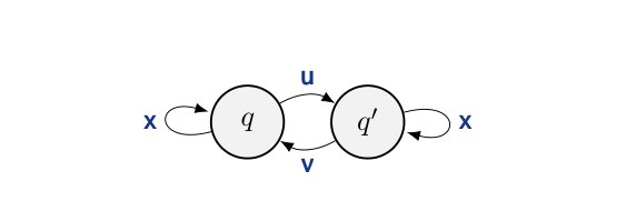
Figure 1: Forbidden configuration in the minimal DFAs of {\color[rgb]{0.4297,0.1172,0.2148}\textup{{LTL}}}\left[{\color[rgb]{0,0.4297,0.2539}\mathrel{\textup{{P}}}},{\color[rgb]{0,0.4297,0.2539}\mathrel{\textup{{Y}}}}\right]-definable languages.
图 1:{\color[rgb]{0.4297,0.1172,0.2148}\textup{{LTL}}}\left[{\color[rgb]{0,0.4297,0.2539}\mathrel{\textup{{P}}}},{\color[rgb]{0,0.4297,0.2539}\mathrel{\textup{{Y}}}}\right] 可定义语言的最小 DFA 中的禁止构型。
Next, we give two examples that respectively illustrate a language definable in {\color[rgb]{0.4297,0.1172,0.2148}\textup{{LTL}}}\left[{\color[rgb]{0,0.4297,0.2539}\mathrel{\textup{{P}}}},{\color[rgb]{0,0.4297,0.2539}\mathrel{\textup{{Y}}}}\right] and a language beyond its expressive power.
接下来我们给出两个例子,分别说明一个能在 {\color[rgb]{0.4297,0.1172,0.2148}\textup{{LTL}}}\left[{\color[rgb]{0,0.4297,0.2539}\mathrel{\textup{{P}}}},{\color[rgb]{0,0.4297,0.2539}\mathrel{\textup{{Y}}}}\right] 中定义的语言,以及一个超出其表达力的语言。
2.4.1 The Locally Testable Languages
The addition of {\color[rgb]{0,0.4297,0.2539}\mathrel{\textup{{Y}}}} enables the definition of classes of languages that are linguistically relevant yet lie beyond the expressive power of {\color[rgb]{0.4297,0.1172,0.2148}\textup{{LTL}}}\left[{\color[rgb]{0,0.4297,0.2539}\mathrel{\textup{{P}}}}\right] alone. As a representative example, we consider the locally testable languages.
2.4.1 局部可检验语言
加入 {\color[rgb]{0,0.4297,0.2539}\mathrel{\textup{{Y}}}} 之后,便能定义一些在语言学上有意义、却超出单独使用 {\color[rgb]{0.4297,0.1172,0.2148}\textup{{LTL}}}\left[{\color[rgb]{0,0.4297,0.2539}\mathrel{\textup{{P}}}}\right] 之表达力的语言类。作为一个有代表性的例子,我们考察局部可检验语言。
A language {{\color[rgb]{0.0781,0.2148,0.5313}L}}\subseteq{{{{\color[rgb]{0.0781,0.2148,0.5313}\Sigma}}^{*}}} is locally -testable, for some , if it is a Boolean combination of languages of the following three forms:
对某个 ,语言 {{\color[rgb]{0.0781,0.2148,0.5313}L}}\subseteq{{{{\color[rgb]{0.0781,0.2148,0.5313}\Sigma}}^{*}}} 是局部 -可检验的,若它是下列三种形式的语言的布尔组合:
\displaystyle\{{{\color[rgb]{0.0781,0.2148,0.5313}\textbf{{w}}}}\in{{{{\color[rgb]{0.0781,0.2148,0.5313}\Sigma}}^{*}}}\mid{{\color[rgb]{0.0781,0.2148,0.5313}\textbf{{u}}}}\in{\mathbb{I}}_{m}({{\color[rgb]{0.0781,0.2148,0.5313}\textbf{{w}}}})\}, \\ \displaystyle{{\color[rgb]{0.0781,0.2148,0.5313}\textbf{{u}}}}\in{{\color[rgb]{0.0781,0.2148,0.5313}\Sigma}}^{m}, \\ \displaystyle\{{{\color[rgb]{0.0781,0.2148,0.5313}\textbf{{w}}}}\in{{{{\color[rgb]{0.0781,0.2148,0.5313}\Sigma}}^{*}}}\mid{P}_{m-1}({{\color[rgb]{0.0781,0.2148,0.5313}\textbf{{w}}}})={{\color[rgb]{0.0781,0.2148,0.5313}\textbf{{u}}}}\}, \\ \displaystyle{{\color[rgb]{0.0781,0.2148,0.5313}\textbf{{u}}}}\in{{\color[rgb]{0.0781,0.2148,0.5313}\Sigma}}^{m-1}, \\ \displaystyle\{{{\color[rgb]{0.0781,0.2148,0.5313}\textbf{{w}}}}\in{{{{\color[rgb]{0.0781,0.2148,0.5313}\Sigma}}^{*}}}\mid{S}_{m-1}({{\color[rgb]{0.0781,0.2148,0.5313}\textbf{{w}}}})={{\color[rgb]{0.0781,0.2148,0.5313}\textbf{{u}}}}\}, \\ \displaystyle{{\color[rgb]{0.0781,0.2148,0.5313}\textbf{{u}}}}\in{{\color[rgb]{0.0781,0.2148,0.5313}\Sigma}}^{m-1}. \tag{1a}
A language is locally testable if it is locally -testable for some . Li and Cotterell (2025) show that {\color[rgb]{0.4297,0.1172,0.2148}\textup{{LTL}}}\left[{\color[rgb]{0,0.4297,0.2539}\mathrel{\textup{{P}}}}\right] cannot define many simple locally testable languages, e.g., {{{{\color[rgb]{0.0781,0.2148,0.5313}\Sigma}}^{*}}}{\color[rgb]{0.0781,0.2148,0.5313}\texttt{a}} and {{{{\color[rgb]{0.0781,0.2148,0.5313}\Sigma}}^{*}}}{\color[rgb]{0.0781,0.2148,0.5313}\texttt{a}}{\color[rgb]{0.0781,0.2148,0.5313}\texttt{b}}{{{{\color[rgb]{0.0781,0.2148,0.5313}\Sigma}}^{*}}}, because they are not right-deterministic. In contrast, as we show in the subsequent theorem, all locally testable languages are definable in {\color[rgb]{0.4297,0.1172,0.2148}\textup{{LTL}}}\left[{\color[rgb]{0,0.4297,0.2539}\mathrel{\textup{{P}}}},{\color[rgb]{0,0.4297,0.2539}\mathrel{\textup{{Y}}}}\right], yielding a witness to the separation in expressive power between {\color[rgb]{0.4297,0.1172,0.2148}\textup{{LTL}}}\left[{\color[rgb]{0,0.4297,0.2539}\mathrel{\textup{{P}}}}\right] and {\color[rgb]{0.4297,0.1172,0.2148}\textup{{LTL}}}\left[{\color[rgb]{0,0.4297,0.2539}\mathrel{\textup{{P}}}},{\color[rgb]{0,0.4297,0.2539}\mathrel{\textup{{Y}}}}\right].
若存在某个 使语言为局部 -可检验的,则称它是局部可检验的。Li and Cotterell (2025) 证明,{\color[rgb]{0.4297,0.1172,0.2148}\textup{{LTL}}}\left[{\color[rgb]{0,0.4297,0.2539}\mathrel{\textup{{P}}}}\right] 无法定义许多简单的局部可检验语言,例如 {{{{\color[rgb]{0.0781,0.2148,0.5313}\Sigma}}^{*}}}{\color[rgb]{0.0781,0.2148,0.5313}\texttt{a}} 与 {{{{\color[rgb]{0.0781,0.2148,0.5313}\Sigma}}^{*}}}{\color[rgb]{0.0781,0.2148,0.5313}\texttt{a}}{\color[rgb]{0.0781,0.2148,0.5313}\texttt{b}}{{{{\color[rgb]{0.0781,0.2148,0.5313}\Sigma}}^{*}}},因为它们不是右确定的。与此相对,如下一定理所示,所有局部可检验语言都能在 {\color[rgb]{0.4297,0.1172,0.2148}\textup{{LTL}}}\left[{\color[rgb]{0,0.4297,0.2539}\mathrel{\textup{{P}}}},{\color[rgb]{0,0.4297,0.2539}\mathrel{\textup{{Y}}}}\right] 中定义,从而为 {\color[rgb]{0.4297,0.1172,0.2148}\textup{{LTL}}}\left[{\color[rgb]{0,0.4297,0.2539}\mathrel{\textup{{P}}}}\right] 与 {\color[rgb]{0.4297,0.1172,0.2148}\textup{{LTL}}}\left[{\color[rgb]{0,0.4297,0.2539}\mathrel{\textup{{P}}}},{\color[rgb]{0,0.4297,0.2539}\mathrel{\textup{{Y}}}}\right] 之间的表达力分离提供了见证。
Theorem 2.8.
Any locally testable language is definable in {\color[rgb]{0.4297,0.1172,0.2148}\textup{{LTL}}}\left[{\color[rgb]{0,0.4297,0.2539}\mathrel{\textup{{P}}}},{\color[rgb]{0,0.4297,0.2539}\mathrel{\textup{{Y}}}}\right].
定理 2.8。
任何局部可检验语言都可以在 {\color[rgb]{0.4297,0.1172,0.2148}\textup{{LTL}}}\left[{\color[rgb]{0,0.4297,0.2539}\mathrel{\textup{{P}}}},{\color[rgb]{0,0.4297,0.2539}\mathrel{\textup{{Y}}}}\right] 中定义。
Proof.
See § C.3. ∎
证明。
见 § C.3。∎
2.4.2 A Bounded Dyck Language
Despite this gain in expressivity, {\color[rgb]{0.4297,0.1172,0.2148}\textup{{LTL}}}\left[{\color[rgb]{0,0.4297,0.2539}\mathrel{\textup{{P}}}},{\color[rgb]{0,0.4297,0.2539}\mathrel{\textup{{Y}}}}\right] still defines a limited class of languages. For instance, it does not define all star-free languages, which are exactly the languages definable in {\color[rgb]{0.4297,0.1172,0.2148}\textup{{LTL}}}[{\color[rgb]{0,0.4297,0.2539}\mathrel{\textup{{S}}}}]. One illustrative family is the bounded Dyck languages, consisting of well-balanced parentheses with a fixed upper bound on nesting depth.[^1] The bounded Dyck language of depth consists of all well-balanced strings whose maximum nesting depth is at most .[^2] For example, over \{{\color[rgb]{0.0781,0.2148,0.5313}\texttt{a}},{\color[rgb]{0.0781,0.2148,0.5313}\texttt{b}}\}, where a is an opening parenthesis and b is a closing parenthesis, the languages
2.4.2 有界 Dyck 语言
尽管表达力有所增强,{\color[rgb]{0.4297,0.1172,0.2148}\textup{{LTL}}}\left[{\color[rgb]{0,0.4297,0.2539}\mathrel{\textup{{P}}}},{\color[rgb]{0,0.4297,0.2539}\mathrel{\textup{{Y}}}}\right] 所能定义的语言类仍然有限。例如,它并不能定义全部无星语言,而无星语言恰好是能在 {\color[rgb]{0.4297,0.1172,0.2148}\textup{{LTL}}}[{\color[rgb]{0,0.4297,0.2539}\mathrel{\textup{{S}}}}] 中定义的那些语言。一个有说明性的家族是有界 Dyck 语言,即嵌套深度有固定上界的良匹配括号。[^1] 深度为 的有界 Dyck 语言,由最大嵌套深度至多为 的全部良匹配字符串组成。[^2] 例如,在 \{{\color[rgb]{0.0781,0.2148,0.5313}\texttt{a}},{\color[rgb]{0.0781,0.2148,0.5313}\texttt{b}}\} 上,其中 a 为开括号、b 为闭括号,语言
{{({\color[rgb]{0.0781,0.2148,0.5313}\texttt{a}}{\color[rgb]{0.0781,0.2148,0.5313}\texttt{b}})^{*}}}\qquad\text{and}\qquad{{({\color[rgb]{0.0781,0.2148,0.5313}\texttt{a}}{{({\color[rgb]{0.0781,0.2148,0.5313}\texttt{a}}{\color[rgb]{0.0781,0.2148,0.5313}\texttt{b}})^{*}}}{\color[rgb]{0.0781,0.2148,0.5313}\texttt{b}})^{*}}} \tag{2}
correspond to maximum nesting depth and .
分别对应最大嵌套深度 与 。
The minimal DFAs for these languages are shown in Fig. 2. The depth- language {{({\color[rgb]{0.0781,0.2148,0.5313}\texttt{a}}{\color[rgb]{0.0781,0.2148,0.5313}\texttt{b}})^{*}}} is recognizable by {\color[rgb]{0.4297,0.1172,0.2148}\textup{{LTL}}}\left[{\color[rgb]{0,0.4297,0.2539}\mathrel{\textup{{P}}}},{\color[rgb]{0,0.4297,0.2539}\mathrel{\textup{{Y}}}}\right], because its minimal DFA avoids the forbidden configuration in Fig. 1. In contrast, the depth- language {{({\color[rgb]{0.0781,0.2148,0.5313}\texttt{a}}{{({\color[rgb]{0.0781,0.2148,0.5313}\texttt{a}}{\color[rgb]{0.0781,0.2148,0.5313}\texttt{b}})^{*}}}{\color[rgb]{0.0781,0.2148,0.5313}\texttt{b}})^{*}}} is not {\color[rgb]{0.4297,0.1172,0.2148}\textup{{LTL}}}\left[{\color[rgb]{0,0.4297,0.2539}\mathrel{\textup{{P}}}},{\color[rgb]{0,0.4297,0.2539}\mathrel{\textup{{Y}}}}\right]-definable: its minimal DFA contains the configuration from Fig. 1, witnessed by , , {{\color[rgb]{0.0781,0.2148,0.5313}\textbf{{u}}}}={\color[rgb]{0.0781,0.2148,0.5313}\texttt{a}}, {{\color[rgb]{0.0781,0.2148,0.5313}\textbf{{v}}}}={\color[rgb]{0.0781,0.2148,0.5313}\texttt{b}}, and {{\color[rgb]{0.0781,0.2148,0.5313}\textbf{{x}}}}={\color[rgb]{0.0781,0.2148,0.5313}\texttt{a}}{\color[rgb]{0.0781,0.2148,0.5313}\texttt{b}}.
这些语言的最小 DFA 见图 2。深度为 1 的语言 {{({\color[rgb]{0.0781,0.2148,0.5313}\texttt{a}}{\color[rgb]{0.0781,0.2148,0.5313}\texttt{b}})^{*}}} 可以被 {\color[rgb]{0.4297,0.1172,0.2148}\textup{{LTL}}}\left[{\color[rgb]{0,0.4297,0.2539}\mathrel{\textup{{P}}}},{\color[rgb]{0,0.4297,0.2539}\mathrel{\textup{{Y}}}}\right] 识别,因为它的最小 DFA 避开了图 1 中的禁止构型。与此相对,深度为 2 的语言 {{({\color[rgb]{0.0781,0.2148,0.5313}\texttt{a}}{{({\color[rgb]{0.0781,0.2148,0.5313}\texttt{a}}{\color[rgb]{0.0781,0.2148,0.5313}\texttt{b}})^{*}}}{\color[rgb]{0.0781,0.2148,0.5313}\texttt{b}})^{*}}} 不能在 {\color[rgb]{0.4297,0.1172,0.2148}\textup{{LTL}}}\left[{\color[rgb]{0,0.4297,0.2539}\mathrel{\textup{{P}}}},{\color[rgb]{0,0.4297,0.2539}\mathrel{\textup{{Y}}}}\right] 中定义:它的最小 DFA 含有图 1 的构型,见证为 ,,{{\color[rgb]{0.0781,0.2148,0.5313}\textbf{{u}}}}={\color[rgb]{0.0781,0.2148,0.5313}\texttt{a}},{{\color[rgb]{0.0781,0.2148,0.5313}\textbf{{v}}}}={\color[rgb]{0.0781,0.2148,0.5313}\texttt{b}},以及 {{\color[rgb]{0.0781,0.2148,0.5313}\textbf{{x}}}}={\color[rgb]{0.0781,0.2148,0.5313}\texttt{a}}{\color[rgb]{0.0781,0.2148,0.5313}\texttt{b}}。
(a) {{({\color[rgb]{0.0781,0.2148,0.5313}\texttt{a}}{\color[rgb]{0.0781,0.2148,0.5313}\texttt{b}})^{*}}}
(b) {{({\color[rgb]{0.0781,0.2148,0.5313}\texttt{a}}{{({\color[rgb]{0.0781,0.2148,0.5313}\texttt{a}}{\color[rgb]{0.0781,0.2148,0.5313}\texttt{b}})^{*}}}{\color[rgb]{0.0781,0.2148,0.5313}\texttt{b}})^{*}}}
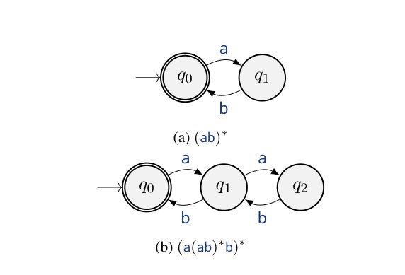
Figure 2: Minimal DFAs. Nodes represent states and arrows represent transitions. The initial state is indicated by an incoming arrow with no source node, and accepting states are shown with double circles.
(a) {{({\color[rgb]{0.0781,0.2148,0.5313}\texttt{a}}{\color[rgb]{0.0781,0.2148,0.5313}\texttt{b}})^{*}}}
(b) {{({\color[rgb]{0.0781,0.2148,0.5313}\texttt{a}}{{({\color[rgb]{0.0781,0.2148,0.5313}\texttt{a}}{\color[rgb]{0.0781,0.2148,0.5313}\texttt{b}})^{*}}}{\color[rgb]{0.0781,0.2148,0.5313}\texttt{b}})^{*}}}
图 2:最小 DFA。节点表示状态,箭头表示转移。初始状态用一条没有源节点的入边标出,接受状态用双圈表示。
2.5 Characterizing {\color[rgb]{0.4297,0.1172,0.2148}\textup{{LTL}}}\left[{\color[rgb]{0,0.4297,0.2539}\mathrel{\textup{{P}}}},{\color[rgb]{0,0.4297,0.2539}\mathrel{\textup{{Y}}}}^{\leq k}\right]
2.5 刻画 {\color[rgb]{0.4297,0.1172,0.2148}\textup{{LTL}}}\left[{\color[rgb]{0,0.4297,0.2539}\mathrel{\textup{{P}}}},{\color[rgb]{0,0.4297,0.2539}\mathrel{\textup{{Y}}}}^{\leq k}\right]
We now introduce two additional temporal operators derived from {\color[rgb]{0,0.4297,0.2539}\mathrel{\textup{{Y}}}}. The bounded operator {\color[rgb]{0,0.4297,0.2539}\mathrel{\textup{{Y}}}}^{\leq k} asks whether {\color[rgb]{0.6875,0.2734,0.1172}\psi} holds at some position among the previous steps, while the unbounded operator {\color[rgb]{0,0.4297,0.2539}\mathrel{\textup{{Y}}}}^{*} asks whether {\color[rgb]{0.6875,0.2734,0.1172}\psi} holds at any earlier position. Formally, these two operators are defined as follows
我们现在引入由 {\color[rgb]{0,0.4297,0.2539}\mathrel{\textup{{Y}}}} 派生的两个额外时序算子。有界算子 {\color[rgb]{0,0.4297,0.2539}\mathrel{\textup{{Y}}}}^{\leq k} 询问 {\color[rgb]{0.6875,0.2734,0.1172}\psi} 是否在此前 步中的某个位置成立,而无界算子 {\color[rgb]{0,0.4297,0.2539}\mathrel{\textup{{Y}}}}^{*} 询问 {\color[rgb]{0.6875,0.2734,0.1172}\psi} 是否在任意更早的位置成立。形式定义如下
\displaystyle{\color[rgb]{0,0.4297,0.2539}\mathrel{\textup{{Y}}}}^{\leq k}{\color[rgb]{0.6875,0.2734,0.1172}\psi} \\ \displaystyle\mathrel{\stackrel{{\scriptstyle\textnormal{def}}}{{=}}}\bigvee_{i=1}^{k}{\color[rgb]{0,0.4297,0.2539}\mathrel{\textup{{Y}}}}^{\,i}{\color[rgb]{0.6875,0.2734,0.1172}\psi}=\bigvee_{i=1}^{k}\underbrace{{\color[rgb]{0,0.4297,0.2539}\mathrel{\textup{{Y}}}}{\color[rgb]{0,0.4297,0.2539}\mathrel{\textup{{Y}}}}\cdots{\color[rgb]{0,0.4297,0.2539}\mathrel{\textup{{Y}}}}}_{i\text{ times}}{\color[rgb]{0.6875,0.2734,0.1172}\psi} \\ \displaystyle{\color[rgb]{0,0.4297,0.2539}\mathrel{\textup{{Y}}}}^{*}{\color[rgb]{0.6875,0.2734,0.1172}\psi} \\ \displaystyle\mathrel{\stackrel{{\scriptstyle\textnormal{def}}}{{=}}}\bigvee_{i=1}^{\infty}{\color[rgb]{0,0.4297,0.2539}\mathrel{\textup{{Y}}}}^{\,i}{\color[rgb]{0.6875,0.2734,0.1172}\psi}=\bigvee_{i=1}^{\infty}\underbrace{{\color[rgb]{0,0.4297,0.2539}\mathrel{\textup{{Y}}}}{\color[rgb]{0,0.4297,0.2539}\mathrel{\textup{{Y}}}}\cdots{\color[rgb]{0,0.4297,0.2539}\mathrel{\textup{{Y}}}}}_{i\text{ times}}{\color[rgb]{0.6875,0.2734,0.1172}\psi} \tag{3a}
Note that {\color[rgb]{0,0.4297,0.2539}\mathrel{\textup{{Y}}}} is the special case {\color[rgb]{0,0.4297,0.2539}\mathrel{\textup{{Y}}}}^{\leq 1}, and {\color[rgb]{0,0.4297,0.2539}\mathrel{\textup{{Y}}}}^{*} coincides with {\color[rgb]{0,0.4297,0.2539}\mathrel{\textup{{P}}}}. This last fact implies that {\color[rgb]{0.4297,0.1172,0.2148}\textup{{LTL}}}[{\color[rgb]{0,0.4297,0.2539}\mathrel{\textup{{P}}}},{\color[rgb]{0,0.4297,0.2539}\mathrel{\textup{{Y}}}}^{*}]={\color[rgb]{0.4297,0.1172,0.2148}\textup{{LTL}}}\left[{\color[rgb]{0,0.4297,0.2539}\mathrel{\textup{{P}}}}\right], i.e., the fragments are not only comparable, they are equivalent. However, for any , the fragment {\color[rgb]{0.4297,0.1172,0.2148}\textup{{LTL}}}\left[{\color[rgb]{0,0.4297,0.2539}\mathrel{\textup{{Y}}}}^{\leq k}\right], as is the case with {\color[rgb]{0.4297,0.1172,0.2148}\textup{{LTL}}}\left[{\color[rgb]{0,0.4297,0.2539}\mathrel{\textup{{Y}}}}\right], is incomparable with {\color[rgb]{0.4297,0.1172,0.2148}\textup{{LTL}}}\left[{\color[rgb]{0,0.4297,0.2539}\mathrel{\textup{{P}}}}\right]. We make this claim precise in the following theorem.
注意 {\color[rgb]{0,0.4297,0.2539}\mathrel{\textup{{Y}}}} 是 {\color[rgb]{0,0.4297,0.2539}\mathrel{\textup{{Y}}}}^{\leq 1} 这一特例,而 {\color[rgb]{0,0.4297,0.2539}\mathrel{\textup{{Y}}}}^{*} 与 {\color[rgb]{0,0.4297,0.2539}\mathrel{\textup{{P}}}} 重合。最后这一事实意味着 {\color[rgb]{0.4297,0.1172,0.2148}\textup{{LTL}}}[{\color[rgb]{0,0.4297,0.2539}\mathrel{\textup{{P}}}},{\color[rgb]{0,0.4297,0.2539}\mathrel{\textup{{Y}}}}^{*}]={\color[rgb]{0.4297,0.1172,0.2148}\textup{{LTL}}}\left[{\color[rgb]{0,0.4297,0.2539}\mathrel{\textup{{P}}}}\right],也就是说这两个片段不仅可比较,而且等价。然而,对任意 ,片段 {\color[rgb]{0.4297,0.1172,0.2148}\textup{{LTL}}}\left[{\color[rgb]{0,0.4297,0.2539}\mathrel{\textup{{Y}}}}^{\leq k}\right] 与 {\color[rgb]{0.4297,0.1172,0.2148}\textup{{LTL}}}\left[{\color[rgb]{0,0.4297,0.2539}\mathrel{\textup{{Y}}}}\right] 一样,与 {\color[rgb]{0.4297,0.1172,0.2148}\textup{{LTL}}}\left[{\color[rgb]{0,0.4297,0.2539}\mathrel{\textup{{P}}}}\right] 不可比。我们把这一论断在下述定理中写精确。
Theorem 2.9.
For any , the fragments {\color[rgb]{0.4297,0.1172,0.2148}\textup{{LTL}}}\left[{\color[rgb]{0,0.4297,0.2539}\mathrel{\textup{{P}}}}\right] and {\color[rgb]{0.4297,0.1172,0.2148}\textup{{LTL}}}\left[{\color[rgb]{0,0.4297,0.2539}\mathrel{\textup{{Y}}}}^{\leq k}\right] are incomparable.
定理 2.9。
对任意 ,片段 {\color[rgb]{0.4297,0.1172,0.2148}\textup{{LTL}}}\left[{\color[rgb]{0,0.4297,0.2539}\mathrel{\textup{{P}}}}\right] 与 {\color[rgb]{0.4297,0.1172,0.2148}\textup{{LTL}}}\left[{\color[rgb]{0,0.4297,0.2539}\mathrel{\textup{{Y}}}}^{\leq k}\right] 不可比。
Proof.
See § C.4. ∎
证明。
见 § C.4。∎
Thus, we arrive at the following corollary.
于是我们得到如下推论。
Corollary 2.10.
The fragment {\color[rgb]{0.4297,0.1172,0.2148}\textup{{LTL}}}\left[{\color[rgb]{0,0.4297,0.2539}\mathrel{\textup{{P}}}},{\color[rgb]{0,0.4297,0.2539}\mathrel{\textup{{Y}}}}^{\leq k}\right] is strictly more expressive than each of the fragments {\color[rgb]{0.4297,0.1172,0.2148}\textup{{LTL}}}\left[{\color[rgb]{0,0.4297,0.2539}\mathrel{\textup{{P}}}}\right] and {\color[rgb]{0.4297,0.1172,0.2148}\textup{{LTL}}}\left[{\color[rgb]{0,0.4297,0.2539}\mathrel{\textup{{Y}}}}^{\leq k}\right].
推论 2.10。
片段 {\color[rgb]{0.4297,0.1172,0.2148}\textup{{LTL}}}\left[{\color[rgb]{0,0.4297,0.2539}\mathrel{\textup{{P}}}},{\color[rgb]{0,0.4297,0.2539}\mathrel{\textup{{Y}}}}^{\leq k}\right] 比 {\color[rgb]{0.4297,0.1172,0.2148}\textup{{LTL}}}\left[{\color[rgb]{0,0.4297,0.2539}\mathrel{\textup{{P}}}}\right] 以及 {\color[rgb]{0.4297,0.1172,0.2148}\textup{{LTL}}}\left[{\color[rgb]{0,0.4297,0.2539}\mathrel{\textup{{Y}}}}^{\leq k}\right] 这两个片段都严格更有表达力。
Proof.
See § C.5. ∎
证明。
见 § C.5。∎
We next analyze expressivity for various ; we find {\color[rgb]{0,0.4297,0.2539}\mathrel{\textup{{Y}}}}^{\leq k} is maximally expressive at .
接下来我们分析各种 下的表达力;我们发现 {\color[rgb]{0,0.4297,0.2539}\mathrel{\textup{{Y}}}}^{\leq k} 在 时表达力最大。
Proposition 2.11.
The fragment {\color[rgb]{0.4297,0.1172,0.2148}\textup{{LTL}}}\left[{\color[rgb]{0,0.4297,0.2539}\mathrel{\textup{{Y}}}}^{\leq k}\right] is strictly less expressive than {\color[rgb]{0.4297,0.1172,0.2148}\textup{{LTL}}}\left[{\color[rgb]{0,0.4297,0.2539}\mathrel{\textup{{Y}}}}\right] for .
命题 2.11。
当 时,片段 {\color[rgb]{0.4297,0.1172,0.2148}\textup{{LTL}}}\left[{\color[rgb]{0,0.4297,0.2539}\mathrel{\textup{{Y}}}}^{\leq k}\right] 比 {\color[rgb]{0.4297,0.1172,0.2148}\textup{{LTL}}}\left[{\color[rgb]{0,0.4297,0.2539}\mathrel{\textup{{Y}}}}\right] 严格更弱。
Proof.
See § C.6. ∎
证明。
见 § C.6。∎
We now show adding {\color[rgb]{0,0.4297,0.2539}\mathrel{\textup{{P}}}} preserves this strictness.
我们现在说明,加入 {\color[rgb]{0,0.4297,0.2539}\mathrel{\textup{{P}}}} 之后,这种严格性仍然保持。
Proposition 2.12.
The fragment {\color[rgb]{0.4297,0.1172,0.2148}\textup{{LTL}}}\left[{\color[rgb]{0,0.4297,0.2539}\mathrel{\textup{{P}}}},{\color[rgb]{0,0.4297,0.2539}\mathrel{\textup{{Y}}}}^{\leq k}\right] is strictly less expressive than {\color[rgb]{0.4297,0.1172,0.2148}\textup{{LTL}}}\left[{\color[rgb]{0,0.4297,0.2539}\mathrel{\textup{{P}}}},{\color[rgb]{0,0.4297,0.2539}\mathrel{\textup{{Y}}}}\right] for .
命题 2.12。
当 时,片段 {\color[rgb]{0.4297,0.1172,0.2148}\textup{{LTL}}}\left[{\color[rgb]{0,0.4297,0.2539}\mathrel{\textup{{P}}}},{\color[rgb]{0,0.4297,0.2539}\mathrel{\textup{{Y}}}}^{\leq k}\right] 比 {\color[rgb]{0.4297,0.1172,0.2148}\textup{{LTL}}}\left[{\color[rgb]{0,0.4297,0.2539}\mathrel{\textup{{P}}}},{\color[rgb]{0,0.4297,0.2539}\mathrel{\textup{{Y}}}}\right] 严格更弱。
Proof.
See § C.7. ∎
证明。
见 § C.7。∎
The gap in expressivity between {\color[rgb]{0.4297,0.1172,0.2148}\textup{{LTL}}}\left[{\color[rgb]{0,0.4297,0.2539}\mathrel{\textup{{P}}}},{\color[rgb]{0,0.4297,0.2539}\mathrel{\textup{{Y}}}}^{\leq k}\right] and {\color[rgb]{0.4297,0.1172,0.2148}\textup{{LTL}}}\left[{\color[rgb]{0,0.4297,0.2539}\mathrel{\textup{{P}}}},{\color[rgb]{0,0.4297,0.2539}\mathrel{\textup{{Y}}}}\right] can, however, be closed in the presence of suitable numerical predicates. Numerical predicates depend only on positions, and not on the tokens occurring at those positions (Straubing, 1994, II.2). A particularly important family is modular predicates , with and :
不过,{\color[rgb]{0.4297,0.1172,0.2148}\textup{{LTL}}}\left[{\color[rgb]{0,0.4297,0.2539}\mathrel{\textup{{P}}}},{\color[rgb]{0,0.4297,0.2539}\mathrel{\textup{{Y}}}}^{\leq k}\right] 与 {\color[rgb]{0.4297,0.1172,0.2148}\textup{{LTL}}}\left[{\color[rgb]{0,0.4297,0.2539}\mathrel{\textup{{P}}}},{\color[rgb]{0,0.4297,0.2539}\mathrel{\textup{{Y}}}}\right] 之间的表达力差距,在具备合适的数值谓词时可以被弥合。数值谓词只依赖于位置,而不依赖于这些位置上出现的词元(Straubing, 1994, II.2)。一类特别重要的是模谓词 ,其中 、:
{{\color[rgb]{0.0781,0.2148,0.5313}\textbf{{w}}}},n\models{\mathrm{MOD}_{m}^{r}}\quad\text{iff}\quad n\equiv r\pmod{m}. \tag{4}
Proposition 2.13.
For every , if modular predicates are available for some , then {\color[rgb]{0.4297,0.1172,0.2148}\textup{{LTL}}}\left[{\color[rgb]{0,0.4297,0.2539}\mathrel{\textup{{Y}}}}^{\leq k}\right] has the same expressive power as {\color[rgb]{0.4297,0.1172,0.2148}\textup{{LTL}}}\left[{\color[rgb]{0,0.4297,0.2539}\mathrel{\textup{{Y}}}}\right], and {\color[rgb]{0.4297,0.1172,0.2148}\textup{{LTL}}}\left[{\color[rgb]{0,0.4297,0.2539}\mathrel{\textup{{P}}}},{\color[rgb]{0,0.4297,0.2539}\mathrel{\textup{{Y}}}}^{\leq k}\right] has the same expressive power as {\color[rgb]{0.4297,0.1172,0.2148}\textup{{LTL}}}\left[{\color[rgb]{0,0.4297,0.2539}\mathrel{\textup{{P}}}},{\color[rgb]{0,0.4297,0.2539}\mathrel{\textup{{Y}}}}\right].
命题 2.13。
对每个 ,若对某个 可以使用模谓词 ,则 {\color[rgb]{0.4297,0.1172,0.2148}\textup{{LTL}}}\left[{\color[rgb]{0,0.4297,0.2539}\mathrel{\textup{{Y}}}}^{\leq k}\right] 与 {\color[rgb]{0.4297,0.1172,0.2148}\textup{{LTL}}}\left[{\color[rgb]{0,0.4297,0.2539}\mathrel{\textup{{Y}}}}\right] 有相同的表达力,且 {\color[rgb]{0.4297,0.1172,0.2148}\textup{{LTL}}}\left[{\color[rgb]{0,0.4297,0.2539}\mathrel{\textup{{P}}}},{\color[rgb]{0,0.4297,0.2539}\mathrel{\textup{{Y}}}}^{\leq k}\right] 与 {\color[rgb]{0.4297,0.1172,0.2148}\textup{{LTL}}}\left[{\color[rgb]{0,0.4297,0.2539}\mathrel{\textup{{P}}}},{\color[rgb]{0,0.4297,0.2539}\mathrel{\textup{{Y}}}}\right] 有相同的表达力。
Proof.
See § C.8. ∎
证明。
见 § C.8。∎
3 The Transformer
3 Transformer
In this section, we formally define the transformer architecture we consider. Note that we analyze the transformer as a language recognizer.
本节我们形式地定义所考虑的 Transformer 结构。需要注意,我们是把 Transformer 作为语言识别器来分析的。
3.1 Preliminaries
3.1 预备知识
All arithmetic in this section is carried out over a set of representable numbers ; we defer the precise formalization to § 3.4. For now, the reader may assume that all relevant operations (addition, multiplication, , etc.) are well-defined over .
本节中的全部算术都在可表示数的集合 上进行;精确的形式化推迟到 § 3.4。眼下,读者可以假定所有相关运算(加法、乘法、 等)在 上都是良定义的。
Definition 3.1(Recognition).
Fix an alphabet {{\color[rgb]{0.0781,0.2148,0.5313}\Sigma}}. A language recognizer is a function ${o}\colon{{{{\color[rgb]{0.0781,0.2148,0.5313}\Sigma}}^{}}}\to{0,1}{{\color[rgb]{0.0781,0.2148,0.5313}L}}\subseteq{{{{\color[rgb]{0.0781,0.2148,0.5313}\Sigma}}^{}}}{o}{o}({{\color[rgb]{0.0781,0.2148,0.5313}\textbf{{w}}}})=1{{\color[rgb]{0.0781,0.2148,0.5313}\textbf{{w}}}}\in{{\color[rgb]{0.0781,0.2148,0.5313}L}}{o}({{\color[rgb]{0.0781,0.2148,0.5313}\textbf{{w}}}})=0{{\color[rgb]{0.0781,0.2148,0.5313}\textbf{{w}}}}\notin{{\color[rgb]{0.0781,0.2148,0.5313}L}}$.
定义 3.1(识别)。
固定字母表 {{\color[rgb]{0.0781,0.2148,0.5313}\Sigma}}。语言识别器是一个函数 {o}\colon{{{{\color[rgb]{0.0781,0.2148,0.5313}\Sigma}}^{*}}}\to\{0,1\}。若对所有 {{\color[rgb]{0.0781,0.2148,0.5313}\textbf{{w}}}}\in{{\color[rgb]{0.0781,0.2148,0.5313}L}} 有 {o}({{\color[rgb]{0.0781,0.2148,0.5313}\textbf{{w}}}})=1,且对所有 {{\color[rgb]{0.0781,0.2148,0.5313}\textbf{{w}}}}\notin{{\color[rgb]{0.0781,0.2148,0.5313}L}} 有 {o}({{\color[rgb]{0.0781,0.2148,0.5313}\textbf{{w}}}})=0,则称语言 {{\color[rgb]{0.0781,0.2148,0.5313}L}}\subseteq{{{{\color[rgb]{0.0781,0.2148,0.5313}\Sigma}}^{*}}} 被 识别。
We can also define string recognition over an eos-extended alphabet {{\overline{{{\color[rgb]{0.0781,0.2148,0.5313}\Sigma}}}}}\mathrel{\stackrel{{\scriptstyle\textnormal{def}}}{{=}}}{{\color[rgb]{0.0781,0.2148,0.5313}\Sigma}}\cup\{{{\textsc{eos}}}\}, where {{\textsc{eos}}}\notin{{\color[rgb]{0.0781,0.2148,0.5313}\Sigma}} is an e****nd-of-sequence token.
我们也可以在 eos 扩充字母表 {{\overline{{{\color[rgb]{0.0781,0.2148,0.5313}\Sigma}}}}}\mathrel{\stackrel{{\scriptstyle\textnormal{def}}}{{=}}}{{\color[rgb]{0.0781,0.2148,0.5313}\Sigma}}\cup\{{{\textsc{eos}}}\} 上定义字符串识别,其中 {{\textsc{eos}}}\notin{{\color[rgb]{0.0781,0.2148,0.5313}\Sigma}} 是一个序列结束词元。
Definition 3.2(eos-Recognition).
Fix an alphabet {{\color[rgb]{0.0781,0.2148,0.5313}\Sigma}}. Let ${o}\colon{{{{\overline{{{\color[rgb]{0.0781,0.2148,0.5313}\Sigma}}}}}^{}}}\to{0,1}{o}{{\color[rgb]{0.0781,0.2148,0.5313}L}}\subseteq{{{{\color[rgb]{0.0781,0.2148,0.5313}\Sigma}}^{}}}{o}{{\color[rgb]{0.0781,0.2148,0.5313}L}}{{\textsc{eos}}}\mathrel{\stackrel{{\scriptstyle\textnormal{def}}}{{=}}}{{{\color[rgb]{0.0781,0.2148,0.5313}\textbf{{w}}}}{{\textsc{eos}}}\mid{{\color[rgb]{0.0781,0.2148,0.5313}\textbf{{w}}}}\in{{\color[rgb]{0.0781,0.2148,0.5313}L}}}\subseteq{{{{\overline{{{\color[rgb]{0.0781,0.2148,0.5313}\Sigma}}}}}^{}}}$.*
定义 3.2(eos 识别)。
固定字母表 {{\color[rgb]{0.0781,0.2148,0.5313}\Sigma}}。设 ${o}\colon{{{{\overline{{{\color[rgb]{0.0781,0.2148,0.5313}\Sigma}}}}}^{}}}\to{0,1}{o}{{\color[rgb]{0.0781,0.2148,0.5313}L}}{{\textsc{eos}}}\mathrel{\stackrel{{\scriptstyle\textnormal{def}}}{{=}}}{{{\color[rgb]{0.0781,0.2148,0.5313}\textbf{{w}}}}{{\textsc{eos}}}\mid{{\color[rgb]{0.0781,0.2148,0.5313}\textbf{{w}}}}\in{{\color[rgb]{0.0781,0.2148,0.5313}L}}}\subseteq{{{{\overline{{{\color[rgb]{0.0781,0.2148,0.5313}\Sigma}}}}}^{*}}}{o}{{\color[rgb]{0.0781,0.2148,0.5313}L}}\subseteq{{{{\color[rgb]{0.0781,0.2148,0.5313}\Sigma}}^{}}}$。
In other words, Definition 3.2 says that, given an input {{\color[rgb]{0.0781,0.2148,0.5313}\textbf{{w}}}}={\color[rgb]{0.0781,0.2148,0.5313}\texttt{w}}_{1}\cdots{\color[rgb]{0.0781,0.2148,0.5313}\texttt{w}}_{N}\in{{{{\color[rgb]{0.0781,0.2148,0.5313}\Sigma}}^{*}}}, the recognizer processes the eos-padded string {{\overline{{{\color[rgb]{0.0781,0.2148,0.5313}\textbf{{w}}}}}}}\mathrel{\stackrel{{\scriptstyle\textnormal{def}}}{{=}}}{\color[rgb]{0.0781,0.2148,0.5313}\texttt{w}}_{1}\cdots{\color[rgb]{0.0781,0.2148,0.5313}\texttt{w}}_{N}{{\textsc{eos}}}. This convention mirrors the semantics of LTL (see § A.3): a formula {\color[rgb]{0.6875,0.2734,0.1172}\psi} is evaluated at position , just beyond the last token of w. In the transformer, position corresponds to eos.
换言之,定义 3.2 是说:给定输入 {{\color[rgb]{0.0781,0.2148,0.5313}\textbf{{w}}}}={\color[rgb]{0.0781,0.2148,0.5313}\texttt{w}}_{1}\cdots{\color[rgb]{0.0781,0.2148,0.5313}\texttt{w}}_{N}\in{{{{\color[rgb]{0.0781,0.2148,0.5313}\Sigma}}^{*}}},识别器处理的是加了 eos 填充的字符串 {{\overline{{{\color[rgb]{0.0781,0.2148,0.5313}\textbf{{w}}}}}}}\mathrel{\stackrel{{\scriptstyle\textnormal{def}}}{{=}}}{\color[rgb]{0.0781,0.2148,0.5313}\texttt{w}}_{1}\cdots{\color[rgb]{0.0781,0.2148,0.5313}\texttt{w}}_{N}{{\textsc{eos}}}。这一约定与 LTL 的语义相呼应(见 § A.3):公式 {\color[rgb]{0.6875,0.2734,0.1172}\psi} 是在位置 处求值的,恰好在 w 最后一个词元之后。在 Transformer 里,位置 就对应 eos。
3.2 Attention
3.2 注意力
The Basic Definition.
Attention can be viewed as a matrix-to-matrix function. Let {{{\color[rgb]{0.3828,0.4492,0.0742}\mathbf{H}}}}\in{\mathbb{F}}^{{D}\times(N+1)} be a matrix. We map {{{\color[rgb]{0.3828,0.4492,0.0742}\mathbf{H}}}} to another matrix as follows. We first define the linear transformations
基本定义。
注意力可以看成一个从矩阵到矩阵的函数。设 {{{\color[rgb]{0.3828,0.4492,0.0742}\mathbf{H}}}}\in{\mathbb{F}}^{{D}\times(N+1)} 为一个矩阵。我们按如下方式把它映到另一个矩阵。首先定义线性变换
\displaystyle{{{\mathbf{Q}}}}({{{\color[rgb]{0.3828,0.4492,0.0742}\mathbf{H}}}}) \\ \displaystyle\mathrel{\stackrel{{\scriptstyle\textnormal{def}}}{{=}}}{\bm{\Theta}^{\text{Q}}}{{{\color[rgb]{0.3828,0.4492,0.0742}\mathbf{H}}}}, \\ \displaystyle{{{\mathbf{K}}}}({{{\color[rgb]{0.3828,0.4492,0.0742}\mathbf{H}}}}) \\ \displaystyle\mathrel{\stackrel{{\scriptstyle\textnormal{def}}}{{=}}}{\bm{\Theta}^{\text{K}}}{{{\color[rgb]{0.3828,0.4492,0.0742}\mathbf{H}}}}, \\ \displaystyle{{{\mathbf{V}}}}({{{\color[rgb]{0.3828,0.4492,0.0742}\mathbf{H}}}}) \\ \displaystyle\mathrel{\stackrel{{\scriptstyle\textnormal{def}}}{{=}}}{\bm{\Theta}^{\text{V}}}{{{\color[rgb]{0.3828,0.4492,0.0742}\mathbf{H}}}}, \tag{5a}
where , , and are parameter matrices. These are often called the q****uery, k****eys and v****alues, respectively. For integers , we then define the s****core as follows
其中 、 和 是参数矩阵。它们通常分别称为查询、键和值。对整数 ,再如下定义分数
{\mathbf{S}}_{n,m}({{{\color[rgb]{0.3828,0.4492,0.0742}\mathbf{H}}}})\mathrel{\stackrel{{\scriptstyle\textnormal{def}}}{{=}}}\frac{{{{\mathbf{Q}}}}_{:,n}({{{\color[rgb]{0.3828,0.4492,0.0742}\mathbf{H}}}})\mathbin{\mathchoice{\hbox to5.74991pt{\hfil\raise 0.0pt\hbox{\scalebox{.5}{\lower 0.0pt\hbox{$\displaystyle\bullet$}}}\hfil}}{\hbox to5.74991pt{\hfil\raise 0.0pt\hbox{\scalebox{.5}{\lower 0.0pt\hbox{$\textstyle\bullet$}}}\hfil}}{\hbox to5.28671pt{\hfil\raise 0.0pt\hbox{\scalebox{.5}{\lower 0.0pt\hbox{$\scriptstyle\bullet$}}}\hfil}}{\hbox to5.1909pt{\hfil\raise 0.0pt\hbox{\scalebox{.5}{\lower 0.0pt\hbox{$\scriptscriptstyle\bullet$}}}\hfil}}}{{{\mathbf{K}}}}_{:,m}({{{\color[rgb]{0.3828,0.4492,0.0742}\mathbf{H}}}})}{\sqrt{{D}_{\text{K}}}}\in{\mathbb{F}}. \\ \textstyle\bullet \tag{6}
Next, we define the ****ttention weights as
接下来,把注意力权重定义为
{\bm{\alpha}}_{n,m}({{{\color[rgb]{0.3828,0.4492,0.0742}\mathbf{H}}}})\mathrel{\stackrel{{\scriptstyle\textnormal{def}}}{{=}}}\frac{\exp({\mathbf{S}}_{n,m}({{{\color[rgb]{0.3828,0.4492,0.0742}\mathbf{H}}}})){\mathbf{M}}_{n,m}}{\sum_{i=1}^{N+1}\exp({\mathbf{S}}_{n,i}({{{\color[rgb]{0.3828,0.4492,0.0742}\mathbf{H}}}})){\mathbf{M}}_{n,i}}, \tag{7}
where is a binary matrix called the m****ask. Note that for all if for all , i.e., if all preceding positions are masked. Finally, we define the resulting matrix
其中 是称为掩码的二元矩阵。注意,若对所有 都有 ,也就是此前位置全部被掩掉,则对所有 有 。最后,定义所得矩阵
{{{\mathbf{O}}}}_{:,n}({{{\color[rgb]{0.3828,0.4492,0.0742}\mathbf{H}}}})\mathrel{\stackrel{{\scriptstyle\textnormal{def}}}{{=}}}\sum_{m=1}^{N+1}{\bm{\alpha}}_{n,m}({{{\color[rgb]{0.3828,0.4492,0.0742}\mathbf{H}}}}){{{\mathbf{V}}}}_{:,m}({{{\color[rgb]{0.3828,0.4492,0.0742}\mathbf{H}}}}), \tag{8}
which is the o****utput of the function. In summary, we define the a****ttention mechanism as follows
它就是该函数的输出。概括起来,我们把注意力机制定义如下
\displaystyle{\mathbf{A}}\colon{\mathbb{F}}^{{D}\times(N+1)} \\ \displaystyle\to{\mathbb{F}}^{{D}\times(N+1)} \\ \displaystyle{{{\color[rgb]{0.3828,0.4492,0.0742}\mathbf{H}}}} \\ \displaystyle\mapsto{{{\mathbf{O}}}}({{{\color[rgb]{0.3828,0.4492,0.0742}\mathbf{H}}}}). \tag{9}
Masking Patterns.
We now give an exposition of several different choices of masks . First, we define the global mask
掩码模式。
下面介绍掩码 的几种不同选择。首先定义全局掩码
$${{{\mathbf{M}}}}^{*}_{n,m}\mathrel{\stackrel{{\scriptstyle\textnormal{def}}}{{=}}}\begin{cases}1&\text{if }m<n,\
0&\text{otherwise.}\end{cases} \tag{10}$$
which corresponds to global attention in the attention mechanism. Next, we define the -local mask:
它在注意力机制中对应全局注意力。接下来定义 -局部掩码:
$$!!{{{\mathbf{M}}}}^{\leq k}_{n,m}\mathrel{\stackrel{{\scriptstyle\textnormal{def}}}{{=}}}\begin{cases}1&\text{if }\max(1,n-k)\leq m<n,\
0&\text{otherwise,}\end{cases} \tag{11}$$
which corresponds to -local attention.
它对应 -局部注意力。
Multi-Head Attention.
It is also commonplace to combine attention heads. A multi-head attention with heads is defined below
多头注意力。
把若干注意力头组合起来也很常见。具有 个头 的多头注意力定义如下
{\mathbf{A}}({{{\color[rgb]{0.3828,0.4492,0.0742}\mathbf{H}}}})\mathrel{\stackrel{{\scriptstyle\textnormal{def}}}{{=}}}\sum_{h=1}^{{H}}{\bm{\Theta}}^{h}{{{\mathbf{O}}}}^{h}({{{\color[rgb]{0.3828,0.4492,0.0742}\mathbf{H}}}}), \tag{12}
where the heads are combined by a linear projection, and each is a parameter. Different heads may use different masks: for instance, some heads may use while others use , giving rise to hybrid global–local attention.
其中各头通过线性投影组合,每个 是一个参数。不同的头可以使用不同的掩码:例如,有的头用 ,有的头用 ,由此得到全局–局部混合注意力。
3.3 Transformer Architecture
3.3 Transformer 结构
We now define a transformer recognizer.
我们现在定义 Transformer 识别器。
Definition 3.3(Transformer).
Fix an alphabet {{\color[rgb]{0.0781,0.2148,0.5313}\Sigma}}. A -transformer is a 4-tuple composed of
定义 3.3(Transformer)。
固定字母表 {{\color[rgb]{0.0781,0.2148,0.5313}\Sigma}}。一个 -Transformer 是由以下部分组成的四元组
- • a token encoder{{{\mathbf{e}}}}\colon{{\overline{{{\color[rgb]{0.0781,0.2148,0.5313}\Sigma}}}}}\to{\mathbb{F}}^{{D}},
- • 词元编码器 {{{\mathbf{e}}}}\colon{{\overline{{{\color[rgb]{0.0781,0.2148,0.5313}\Sigma}}}}}\to{\mathbb{F}}^{{D}},
- • a family of attention mechanisms,
- • 一族注意力机制 ,
- • a family of non-linear functionswhere each, and
- • 一族非线性函数 ,其中每个 ,以及
- • a classification function.
- • 一个分类函数 。
A transformer eos-recognizes a language as follows. Given {{\overline{{{\color[rgb]{0.0781,0.2148,0.5313}\textbf{{w}}}}}}}={\color[rgb]{0.0781,0.2148,0.5313}\texttt{w}}_{1}\cdots{\color[rgb]{0.0781,0.2148,0.5313}\texttt{w}}_{N}{{\textsc{eos}}} where {\color[rgb]{0.0781,0.2148,0.5313}\texttt{w}}_{1},\ldots,{\color[rgb]{0.0781,0.2148,0.5313}\texttt{w}}_{N}\in{{\color[rgb]{0.0781,0.2148,0.5313}\Sigma}}, define the base case
Transformer 按如下方式 eos 识别一个语言。给定 {{\overline{{{\color[rgb]{0.0781,0.2148,0.5313}\textbf{{w}}}}}}}={{\color[rgb]{0.0781,0.2148,0.5313}\texttt{w}}_{1}\cdots{\color[rgb]{0.0781,0.2148,0.5313}\texttt{w}}_{N}{{\textsc{eos}}},其中 {\color[rgb]{0.0781,0.2148,0.5313}\texttt{w}}_{1},\ldots,{\color[rgb]{0.0781,0.2148,0.5313}\texttt{w}}_{N}\in{{\color[rgb]{0.0781,0.2148,0.5313}\Sigma}},定义基础情形
{{{{\color[rgb]{0.3828,0.4492,0.0742}\mathbf{H}}}}^{0}({{\overline{{{\color[rgb]{0.0781,0.2148,0.5313}\textbf{{w}}}}}}})_{:,n}}\mathrel{\stackrel{{\scriptstyle\textnormal{def}}}{{=}}}{{{\mathbf{e}}}}({\color[rgb]{0.0781,0.2148,0.5313}\texttt{w}}_{n}),\quad\forall n\in\{1,\ldots,N+1\}. \tag{13}
Then, for each layer , compute
然后,对每一层 ,计算
\displaystyle{{{{\mathbf{G}}}}^{\ell}({{\overline{{{\color[rgb]{0.0781,0.2148,0.5313}\textbf{{w}}}}}}})} \\ \displaystyle\mathrel{\stackrel{{\scriptstyle\textnormal{def}}}{{=}}}{\text{LN}}\left({{{{\color[rgb]{0.3828,0.4492,0.0742}\mathbf{H}}}}^{\ell-1}({{\overline{{{\color[rgb]{0.0781,0.2148,0.5313}\textbf{{w}}}}}}})}+{\mathbf{A}^{\ell}}({{{{\color[rgb]{0.3828,0.4492,0.0742}\mathbf{H}}}}^{\ell-1}({{\overline{{{\color[rgb]{0.0781,0.2148,0.5313}\textbf{{w}}}}}}})})\right), \\ \displaystyle{{{{\color[rgb]{0.3828,0.4492,0.0742}\mathbf{H}}}}^{\ell}({{\overline{{{\color[rgb]{0.0781,0.2148,0.5313}\textbf{{w}}}}}}})} \\ \displaystyle\mathrel{\stackrel{{\scriptstyle\textnormal{def}}}{{=}}}{\text{LN}}\left({{{{\mathbf{G}}}}^{\ell}({{\overline{{{\color[rgb]{0.0781,0.2148,0.5313}\textbf{{w}}}}}}})}+{\mathbf{F}^{\ell}}({{{{\mathbf{G}}}}^{\ell}({{\overline{{{\color[rgb]{0.0781,0.2148,0.5313}\textbf{{w}}}}}}})})\right), \tag{14a}
where is applied column-wise, and LN is layer normalization (Ba et al., 2016). The transformer’s output is then {o}({{\color[rgb]{0.0781,0.2148,0.5313}\textbf{{w}}}})\mathrel{\stackrel{{\scriptstyle\textnormal{def}}}{{=}}}{c}({{{{\color[rgb]{0.3828,0.4492,0.0742}\mathbf{H}}}}^{{L}}({{\overline{{{\color[rgb]{0.0781,0.2148,0.5313}\textbf{{w}}}}}}})_{:,N+1}}).
其中 按列作用,LN 是层归一化(Ba et al., 2016)。Transformer 的输出则为 {o}({{\color[rgb]{0.0781,0.2148,0.5313}\textbf{{w}}}})\mathrel{\stackrel{{\scriptstyle\textnormal{def}}}{{=}}}{c}({{{{\color[rgb]{0.3828,0.4492,0.0742}\mathbf{H}}}}^{{L}}({{\overline{{{\color[rgb]{0.0781,0.2148,0.5313}\textbf{{w}}}}}}})_{:,N+1}})。
3.4 Fixed Precision
3.4 固定精度
In the exposition above, we assumed that transformers operate at fixed precision, i.e., there exists a finite set of numbers—analogous to the floating-point formats used in practice (IEEE, 2019)—such that all parameters and intermediate values lie in . Every primitive operation, including and the division in softmax, is performed in and rounded back into . We note that fixed-precision arithmetic differs from exact arithmetic in subtle ways: for instance, addition is not generally associative over , so the order of summation in softmax can affect the result. Nevertheless, the fixed-precision assumption is standard in the analysis of transformers and is part of what makes the connection to finite automata and temporal logic possible.
在上面的叙述中,我们假定 Transformer 在固定精度下运算,也就是说,存在一个有限的数集 ——类似于实践中使用的浮点格式(IEEE, 2019)——使得全部参数与中间值都落在 中。每一个原语运算,包括 以及 softmax 中的除法,都在 中执行,并再舍入回 。需要指出,固定精度算术与精确算术有一些细微差别:例如,加法在 上一般不满足结合律,因而 softmax 中求和的次序可能影响结果。尽管如此,固定精度假定在 Transformer 分析中是标准做法,也正是它使与有限自动机和时序逻辑的联系成为可能。
4 Characterizing Transformers
4 刻画 Transformer
We now show that global, local, and hybrid attention correspond exactly to the fragments introduced in § 2. We first restate an existing result, relating transformers with global attention to {\color[rgb]{0.4297,0.1172,0.2148}\textup{{LTL}}}\left[{\color[rgb]{0,0.4297,0.2539}\mathrel{\textup{{P}}}}\right].
我们现在说明,全局、局部与混合注意力恰好对应第 2 节引入的那些片段。先重述一个已有结果,它把带全局注意力的 Transformer 与 {\color[rgb]{0.4297,0.1172,0.2148}\textup{{LTL}}}\left[{\color[rgb]{0,0.4297,0.2539}\mathrel{\textup{{P}}}}\right] 联系起来。
Theorem 4.1(Li and Cotterell, 2025).
A language {{\color[rgb]{0.0781,0.2148,0.5313}L}} is eos-recognizable by a -transformer in which every attention head uses the global mask ${{{\mathbf{M}}}}^{}{\color[rgb]{0.4297,0.1172,0.2148}\textup{{LTL}}}\left[{\color[rgb]{0,0.4297,0.2539}\mathrel{\textup{{P}}}}\right]$.*
定理 4.1(Li and Cotterell, 2025)。
语言 {{\color[rgb]{0.0781,0.2148,0.5313}L}} 可被一个每个注意力头都使用全局掩码 ${{{\mathbf{M}}}}^{}({D},{L})\bigl({{{\mathbf{e}}}},{{\mathbf{A}^{\ell}}}{\ell=1}^{{L}},{{\mathbf{F}^{\ell}}}{\ell=1}^{{L}},{c}\bigr){\color[rgb]{0.4297,0.1172,0.2148}\textup{{LTL}}}\left[{\color[rgb]{0,0.4297,0.2539}\mathrel{\textup{{P}}}}\right]$ 中定义。*
We now consider -local attention.
我们现在考虑 -局部注意力。
Theorem 4.2.
A language {{\color[rgb]{0.0781,0.2148,0.5313}L}} is eos-recognizable by a -transformer in which every attention head uses the -local mask if and only if it is definable in {\color[rgb]{0.4297,0.1172,0.2148}\textup{{LTL}}}\left[{\color[rgb]{0,0.4297,0.2539}\mathrel{\textup{{Y}}}}^{\leq k}\right].
定理 4.2。
语言 {{\color[rgb]{0.0781,0.2148,0.5313}L}} 可被一个每个注意力头都使用 -局部掩码 的 -Transformer eos 识别,当且仅当它可在 {\color[rgb]{0.4297,0.1172,0.2148}\textup{{LTL}}}\left[{\color[rgb]{0,0.4297,0.2539}\mathrel{\textup{{Y}}}}^{\leq k}\right] 中定义。
Proof sketch.
The argument follows the same structure as Li and Cotterell (2025) for Theorem 4.1. Because each query attends to at most predecessors, all summations in the masked softmax and value aggregation reduce to bounded counting, which is expressible in {\color[rgb]{0.4297,0.1172,0.2148}\textup{{LTL}}}\left[{\color[rgb]{0,0.4297,0.2539}\mathrel{\textup{{Y}}}}^{\leq k}\right] using bounded nesting of {\color[rgb]{0,0.4297,0.2539}\mathrel{\textup{{Y}}}}^{\leq k}. Conversely, by induction on {\color[rgb]{0.4297,0.1172,0.2148}\textup{{LTL}}}\left[{\color[rgb]{0,0.4297,0.2539}\mathrel{\textup{{Y}}}}^{\leq k}\right] formulas, Boolean connectives are implemented positionwise, and {\color[rgb]{0,0.4297,0.2539}\mathrel{\textup{{Y}}}}^{\leq k}{\color[rgb]{0.6875,0.2734,0.1172}\psi} is realized by a -local attention head that aggregates information from the last positions satisfying {\color[rgb]{0.6875,0.2734,0.1172}\psi}. The same refinement step as in Li and Cotterell (2025, Lemma B.12) can be applied. ∎
证明梗概。
论证的结构与 Li and Cotterell (2025) 对定理 4.1 的处理相同。由于每个查询至多关注 个前驱,带掩码的 softmax 与值聚合中的全部求和都化为有界计数,而这可以用 {\color[rgb]{0,0.4297,0.2539}\mathrel{\textup{{Y}}}}^{\leq k} 的有界嵌套在 {\color[rgb]{0.4297,0.1172,0.2148}\textup{{LTL}}}\left[{\color[rgb]{0,0.4297,0.2539}\mathrel{\textup{{Y}}}}^{\leq k}\right] 中表达。反过来,对 {\color[rgb]{0.4297,0.1172,0.2148}\textup{{LTL}}}\left[{\color[rgb]{0,0.4297,0.2539}\mathrel{\textup{{Y}}}}^{\leq k}\right] 公式做归纳:布尔联结词按位置实现,而 {\color[rgb]{0,0.4297,0.2539}\mathrel{\textup{{Y}}}}^{\leq k}{\color[rgb]{0.6875,0.2734,0.1172}\psi} 由一个 -局部注意力头实现,该头从满足 {\color[rgb]{0.6875,0.2734,0.1172}\psi} 的最近 个位置聚合信息。Li and Cotterell (2025, Lemma B.12) 中的同样精细化步骤也可以使用。∎
Finally, we consider hybrid transformers that mix global and -local heads.
最后,我们考虑把全局头与 -局部头混合起来的混合 Transformer。
Theorem 4.3.
A language {{\color[rgb]{0.0781,0.2148,0.5313}L}} is eos-recognizable by a -transformer in which some heads use ${{{\mathbf{M}}}}^{}{{{\mathbf{M}}}}^{\leq k}{\color[rgb]{0.4297,0.1172,0.2148}\textup{{LTL}}}\left[{\color[rgb]{0,0.4297,0.2539}\mathrel{\textup{{P}}}},{\color[rgb]{0,0.4297,0.2539}\mathrel{\textup{{Y}}}}^{\leq k}\right]$.*
定理 4.3。
语言 {{\color[rgb]{0.0781,0.2148,0.5313}L}} 可被一个部分头使用 ${{{\mathbf{M}}}}^{}{{{\mathbf{M}}}}^{\leq k}({D},{L})\bigl({{{\mathbf{e}}}},{{\mathbf{A}^{\ell}}}{\ell=1}^{{L}},{{\mathbf{F}^{\ell}}}{\ell=1}^{{L}},{c}\bigr){\color[rgb]{0.4297,0.1172,0.2148}\textup{{LTL}}}\left[{\color[rgb]{0,0.4297,0.2539}\mathrel{\textup{{P}}}},{\color[rgb]{0,0.4297,0.2539}\mathrel{\textup{{Y}}}}^{\leq k}\right]$ 中定义。*
Proof.
The theorem is a direct corollary of Theorems 4.1 and 4.2. ∎
证明。
本定理是定理 4.1 与定理 4.2 的直接推论。∎
4.1 Outlook
4.1 展望
We now translate the logical characterizations into concrete consequences for transformers under different attention patterns. An immediate consequence of Theorems 4.1, 4.2 and 4.3 together with Corollary 2.10 is that transformers with hybrid global-local attention are strictly more expressive than either global-only or -local-only transformers. Thus, mixing local and global attention is not only computationally attractive (Luong et al., 2015; Child et al., 2019; Beltagy et al., 2020; Zaheer et al., 2020), but can also yield a strict expressive gain. Moreover, -local attention is the strongest choice within the local-attention family: by Propositions 2.11, 2.12, 4.2 and 4.3, for every , transformers with -local attention are strictly more expressive than those with -local attention, and the same holds when global heads are added. This suggests that 1-local attention is a particularly promising choice in practice. We note, however, two important caveats.
我们现在把逻辑上的刻画转成对不同注意力模式的 Transformer 的具体推论。定理 4.1、4.2 与 4.3 再加上推论 2.10,立刻得到:带全局–局部混合注意力的 Transformer,比只使用全局或只使用 -局部的 Transformer 都严格更有表达力。因此,把局部与全局注意力混合起来,不仅在计算上有吸引力(Luong et al., 2015; Child et al., 2019; Beltagy et al., 2020; Zaheer et al., 2020),还可以带来严格的表达力增益。此外,在局部注意力这一族里,-局部注意力是最强的选择:由命题 2.11、2.12 以及定理 4.2 与 4.3,对每个 ,带 -局部注意力的 Transformer 都比带 -局部注意力的严格更有表达力,在再加入全局头时也是如此。这提示 -局部注意力在实践中是一个特别值得考虑的选择。不过,有两点重要的保留需要说明。
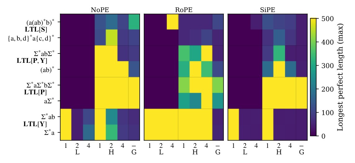
Figure 3: Heatmap of longest perfect lengths (maximum over runs) across formal languages, attention patterns, and positional encodings. Columns denote local (L), hybrid (H), and global (G) attention patterns; for L and H, the labels above columns indicate the local window size .
图 3:在各形式语言、注意力模式与位置编码上,最长完美长度(各次运行取最大)的热图。各列表示局部(L)、混合(H)与全局(G)注意力模式;对 L 与 H,列上方的标签给出局部窗口大小 。
Depth Overhead.
Although -local attention maximizes expressivity, replacing a single -local head by -local heads may incur a depth overhead. At the logical level, expressing {\color[rgb]{0,0.4297,0.2539}\mathrel{\textup{{Y}}}}^{\leq k}{\color[rgb]{0.6875,0.2734,0.1172}\psi} via Eq. 3a requires a disjunction of formulas of the form {\color[rgb]{0,0.4297,0.2539}\mathrel{\textup{{Y}}}}^{i}{\color[rgb]{0.6875,0.2734,0.1172}\psi} for . Thus, using only {\color[rgb]{0,0.4297,0.2539}\mathrel{\textup{{Y}}}} increases the operator depth (§ A.2) from {\text{od}}({\color[rgb]{0.6875,0.2734,0.1172}\psi})+1 to as much as {\text{od}}({\color[rgb]{0.6875,0.2734,0.1172}\psi})+k. In other words, eliminating {\color[rgb]{0,0.4297,0.2539}\mathrel{\textup{{Y}}}}^{\leq k} in favor of {\color[rgb]{0,0.4297,0.2539}\mathrel{\textup{{Y}}}} preserves expressivity, but may increase the required depth by an overhead of up to . Specifically, in the proof of Theorem 4.2, each temporal operator requires at least one layer to simulate, so this translation may require up to stacked layers in place of a single layer. Thus, under a fixed depth, transformers with -local attention need not be strictly more expressive than transformers with -local attention. In practice, modern language models are deep (OpenAI, 2023), making this limitation less of a practical detriment and rendering architectures with -local heads a plausible way to increase expressivity.
深度开销。
尽管 -局部注意力使表达力达到最大,用若干 -局部头替换单个 -局部头可能会带来深度开销。在逻辑层面,经由式 3a 来表达 {\color[rgb]{0,0.4297,0.2539}\mathrel{\textup{{Y}}}}^{\leq k}{\color[rgb]{0.6875,0.2734,0.1172}\psi},需要一组形如 {\color[rgb]{0,0.4297,0.2539}\mathrel{\textup{{Y}}}}^{i}{\color[rgb]{0.6875,0.2734,0.1172}\psi}()的公式的析取。因此,只使用 {\color[rgb]{0,0.4297,0.2539}\mathrel{\textup{{Y}}}} 会把算子深度(§ A.2)从 {\text{od}}({\color[rgb]{0.6875,0.2734,0.1172}\psi})+1 提高到至多 {\text{od}}({\color[rgb]{0.6875,0.2734,0.1172}\psi})+k。换言之,用 {\color[rgb]{0,0.4297,0.2539}\mathrel{\textup{{Y}}}} 消去 {\color[rgb]{0,0.4297,0.2539}\mathrel{\textup{{Y}}}}^{\leq k} 可以保持表达力,却可能把所需深度提高至多 。具体来说,在定理 4.2 的证明中,每个时序算子至少需要一层来模拟,因而这一改写可能要用多达 层叠起来的层,去替换原来的单层。因此,在深度固定时,带 -局部注意力的 Transformer 不必比带 -局部注意力的严格更有表达力。实践中,现代语言模型通常很深(OpenAI, 2023),这一限制的实际损害较小,带 -局部头的结构仍是提高表达力的一条可行路径。
Positional Encodings.
The strict separation above holds in the absence of positional encodings. With sufficiently rich positional information, however, the gap can disappear. Intuitively, if the model can always identify the immediate predecessor within a -window, then -local attention can simulate -local attention. Positional encodings are often viewed as numerical predicates added to the logic (Yang et al., 2024; Li and Cotterell, 2025). By Proposition 2.13, suitable modular predicates suffice to erase the gap. Therefore, if positional encodings that simulate such predicates are available, then a -local head can recover the immediate predecessor by selecting, at each position, the unique position in the previous steps. Interestingly, sinusoidal encodings (SiPE; Vaswani et al. 2017) and rotary encodings (RoPE; Su et al. 2024) can be related to modular predicates (Yang et al., 2025). However, realizing modular predicates in this way requires a rational variant (Chiang et al., 2023), which is not the form typically used in practice.
位置编码。
上述严格分离是在没有位置编码的条件下成立的。不过,若位置信息足够丰富,这一差距可以消失。直观上,只要模型总能在一个 -窗口内认出紧邻的前驱,则 -局部注意力就可以模拟 -局部注意力。位置编码常常被看成加入逻辑中的数值谓词(Yang et al., 2024; Li and Cotterell, 2025)。由命题 2.13,合适的模谓词就足以抹平这一差距。因此,若可以使用能够模拟这类谓词的位置编码,则一个 -局部头可以通过在每个位置选出此前 步中那个唯一的位置,来恢复紧邻前驱。有意思的是,正弦编码(SiPE; Vaswani et al. 2017)与旋转编码(RoPE; Su et al. 2024)都可以与模谓词联系起来(Yang et al., 2025)。不过,以这种方式实现模谓词需要一种有理数变体(Chiang et al., 2023),而这并不是实践中通常采用的形式。
5 Empirically Verifying the Theory
5 从经验上核验理论
In this section, we test the expressivity predictions of our theory on formal language recognition tasks.
本节我们在形式语言识别任务上检验理论关于表达力的预测。
5.1 Languages
5.1 语言
We evaluate a suite of formal languages grouped by definability in temporal-logic fragments, selecting two representative languages from each class:
我们评估一套按在时序逻辑片段中可否定义来分组的形式语言,并从每一类中选取两个有代表性的语言:
- • {\color[rgb]{0.4297,0.1172,0.2148}\textup{{LTL}}}\left[{\color[rgb]{0,0.4297,0.2539}\mathrel{\textup{{Y}}}}\right]-definable: {{{{\color[rgb]{0.0781,0.2148,0.5313}\Sigma}}^{*}}}{\color[rgb]{0.0781,0.2148,0.5313}\texttt{a}} (strings ending with a) and {{{{\color[rgb]{0.0781,0.2148,0.5313}\Sigma}}^{*}}}{\color[rgb]{0.0781,0.2148,0.5313}\texttt{a}}{\color[rgb]{0.0781,0.2148,0.5313}\texttt{b}} (strings ending with ab).
- • 可在 {\color[rgb]{0.4297,0.1172,0.2148}\textup{{LTL}}}\left[{\color[rgb]{0,0.4297,0.2539}\mathrel{\textup{{Y}}}}\right] 中定义:{{{{\color[rgb]{0.0781,0.2148,0.5313}\Sigma}}^{*}}}{\color[rgb]{0.0781,0.2148,0.5313}\texttt{a}}(以 a 结尾的字符串)以及 {{{{\color[rgb]{0.0781,0.2148,0.5313}\Sigma}}^{*}}}{\color[rgb]{0.0781,0.2148,0.5313}\texttt{a}}{\color[rgb]{0.0781,0.2148,0.5313}\texttt{b}}(以 ab 结尾的字符串)。
- • {\color[rgb]{0.4297,0.1172,0.2148}\textup{{LTL}}}\left[{\color[rgb]{0,0.4297,0.2539}\mathrel{\textup{{P}}}}\right]-definable: {\color[rgb]{0.0781,0.2148,0.5313}\texttt{a}}{{{{\color[rgb]{0.0781,0.2148,0.5313}\Sigma}}^{*}}} (strings starting with a) and {{{{\color[rgb]{0.0781,0.2148,0.5313}\Sigma}}^{*}}}{\color[rgb]{0.0781,0.2148,0.5313}\texttt{a}}{{{{\color[rgb]{0.0781,0.2148,0.5313}\Sigma}}^{*}}}{\color[rgb]{0.0781,0.2148,0.5313}\texttt{b}}{{{{\color[rgb]{0.0781,0.2148,0.5313}\Sigma}}^{*}}} (strings containing ab as a not-necessarily-contiguous subsequence).
- • 可在 {\color[rgb]{0.4297,0.1172,0.2148}\textup{{LTL}}}\left[{\color[rgb]{0,0.4297,0.2539}\mathrel{\textup{{P}}}}\right] 中定义:{\color[rgb]{0.0781,0.2148,0.5313}\texttt{a}}{{{{\color[rgb]{0.0781,0.2148,0.5313}\Sigma}}^{*}}}(以 a 开头的字符串)以及 {{{{\color[rgb]{0.0781,0.2148,0.5313}\Sigma}}^{*}}}{\color[rgb]{0.0781,0.2148,0.5313}\texttt{a}}{{{{\color[rgb]{0.0781,0.2148,0.5313}\Sigma}}^{*}}}{\color[rgb]{0.0781,0.2148,0.5313}\texttt{b}}{{{{\color[rgb]{0.0781,0.2148,0.5313}\Sigma}}^{*}}}(把 ab 作为不必连续的子序列含在其中的字符串)。
- • {\color[rgb]{0.4297,0.1172,0.2148}\textup{{LTL}}}\left[{\color[rgb]{0,0.4297,0.2539}\mathrel{\textup{{P}}}},{\color[rgb]{0,0.4297,0.2539}\mathrel{\textup{{Y}}}}\right]-definable but not in {\color[rgb]{0.4297,0.1172,0.2148}\textup{{LTL}}}\left[{\color[rgb]{0,0.4297,0.2539}\mathrel{\textup{{P}}}}\right] or {\color[rgb]{0.4297,0.1172,0.2148}\textup{{LTL}}}\left[{\color[rgb]{0,0.4297,0.2539}\mathrel{\textup{{Y}}}}\right]: {{({\color[rgb]{0.0781,0.2148,0.5313}\texttt{a}}{\color[rgb]{0.0781,0.2148,0.5313}\texttt{b}})^{*}}} (strings of repeated ab) and {{{{\color[rgb]{0.0781,0.2148,0.5313}\Sigma}}^{*}}}{\color[rgb]{0.0781,0.2148,0.5313}\texttt{a}}{\color[rgb]{0.0781,0.2148,0.5313}\texttt{b}}{{{{\color[rgb]{0.0781,0.2148,0.5313}\Sigma}}^{*}}} (strings containing ab as a contiguous substring).
- • 可在 {\color[rgb]{0.4297,0.1172,0.2148}\textup{{LTL}}}\left[{\color[rgb]{0,0.4297,0.2539}\mathrel{\textup{{P}}}},{\color[rgb]{0,0.4297,0.2539}\mathrel{\textup{{Y}}}}\right] 中定义,但不能在 {\color[rgb]{0.4297,0.1172,0.2148}\textup{{LTL}}}\left[{\color[rgb]{0,0.4297,0.2539}\mathrel{\textup{{P}}}}\right] 或 {\color[rgb]{0.4297,0.1172,0.2148}\textup{{LTL}}}\left[{\color[rgb]{0,0.4297,0.2539}\mathrel{\textup{{Y}}}}\right] 中定义:{{({\color[rgb]{0.0781,0.2148,0.5313}\texttt{a}}{\color[rgb]{0.0781,0.2148,0.5313}\texttt{b}})^{*}}}(由重复的 ab 构成的字符串)以及 {{{{\color[rgb]{0.0781,0.2148,0.5313}\Sigma}}^{*}}}{\color[rgb]{0.0781,0.2148,0.5313}\texttt{a}}{\color[rgb]{0.0781,0.2148,0.5313}\texttt{b}}{{{{\color[rgb]{0.0781,0.2148,0.5313}\Sigma}}^{*}}}(把 ab 作为连续子串含在其中的字符串)。
- • {\color[rgb]{0.4297,0.1172,0.2148}\textup{{LTL}}}[{\color[rgb]{0,0.4297,0.2539}\mathrel{\textup{{S}}}}]-definable but not in {\color[rgb]{0.4297,0.1172,0.2148}\textup{{LTL}}}\left[{\color[rgb]{0,0.4297,0.2539}\mathrel{\textup{{P}}}},{\color[rgb]{0,0.4297,0.2539}\mathrel{\textup{{Y}}}}\right]: {{\{{\color[rgb]{0.0781,0.2148,0.5313}\texttt{a}},{\color[rgb]{0.0781,0.2148,0.5313}\texttt{b}},{\color[rgb]{0.0781,0.2148,0.5313}\texttt{d}}\}^{*}}}{\color[rgb]{0.0781,0.2148,0.5313}\texttt{a}}{{\{{\color[rgb]{0.0781,0.2148,0.5313}\texttt{c}},{\color[rgb]{0.0781,0.2148,0.5313}\texttt{d}}\}^{*}}} (a right-deterministic polynomial) and {{({\color[rgb]{0.0781,0.2148,0.5313}\texttt{a}}{{({\color[rgb]{0.0781,0.2148,0.5313}\texttt{a}}{\color[rgb]{0.0781,0.2148,0.5313}\texttt{b}})^{*}}}{\color[rgb]{0.0781,0.2148,0.5313}\texttt{b}})^{*}}} (bounded Dyck with maximum nesting depth ).
- • 可在 {\color[rgb]{0.4297,0.1172,0.2148}\textup{{LTL}}}[{\color[rgb]{0,0.4297,0.2539}\mathrel{\textup{{S}}}}] 中定义,但不能在 {\color[rgb]{0.4297,0.1172,0.2148}\textup{{LTL}}}\left[{\color[rgb]{0,0.4297,0.2539}\mathrel{\textup{{P}}}},{\color[rgb]{0,0.4297,0.2539}\mathrel{\textup{{Y}}}}\right] 中定义:{{\{{\color[rgb]{0.0781,0.2148,0.5313}\texttt{a}},{\color[rgb]{0.0781,0.2148,0.5313}\texttt{b}},{\color[rgb]{0.0781,0.2148,0.5313}\texttt{d}}\}^{*}}}{\color[rgb]{0.0781,0.2148,0.5313}\texttt{a}}{{\{{\color[rgb]{0.0781,0.2148,0.5313}\texttt{c}},{\color[rgb]{0.0781,0.2148,0.5313}\texttt{d}}\}^{*}}}(一个右确定多项式)以及 {{({\color[rgb]{0.0781,0.2148,0.5313}\texttt{a}}{{({\color[rgb]{0.0781,0.2148,0.5313}\texttt{a}}{\color[rgb]{0.0781,0.2148,0.5313}\texttt{b}})^{*}}}{\color[rgb]{0.0781,0.2148,0.5313}\texttt{b}})^{*}}}(最大嵌套深度为 的有界 Dyck)。
5.2 Experimental Setup
5.2 实验设置
We consider three attention settings, corresponding to the masking patterns defined in § 3: local-only (all heads use ), hybrid (half the heads use , the rest use ), and global-only (all heads use ). For local-only and hybrid models, we vary the window size . We also evaluate transformers with two positional encodings: sinusoidal encodings (SiPE; Vaswani et al. 2017) and rotary encodings (RoPE; Su et al. 2024). The models are trained on strings of length up to and evaluated on lengths –. Each experiment is run with random seeds and learning rates; additional details are given in § D.2. In addition to accuracy, we report the longest perfect length, defined as the largest length up to which the model achieves accuracy.
我们考虑三种注意力设定,对应第 3 节定义的掩码模式:仅局部(所有头使用 )、混合(一半头使用 ,其余使用 )以及仅全局(所有头使用 )。对仅局部与混合模型,我们改变窗口大小 。我们也评估配备两种位置编码的 Transformer:正弦编码(SiPE; Vaswani et al. 2017)与旋转编码(RoPE; Su et al. 2024)。模型在长度至多为 的字符串上训练,并在长度 – 上评估。每项实验使用 个随机种子与 个学习率;更多细节见 § D.2。除准确率外,我们还报告最长完美长度,即模型准确率达到 的最大长度。
5.3 Results
5.3 结果
We summarize performance using a heatmap of the longest perfect length in Fig. 3. Full numerical results, including accuracies and longest perfect lengths, are provided in § D.3.
我们用图 3 中最长完美长度的热图来概括表现。完整数值结果,包括准确率与最长完美长度,见 § D.3。
5.3.1 Results on NoPE
We begin with a discussion of the NoPE setting, whose results are shown on the left panel of Fig. 3.
5.3.1 无位置编码(NoPE)上的结果
我们先讨论 NoPE 设定,其结果见图 3 左侧面板。
Local-only models match {\color[rgb]{0.4297,0.1172,0.2148}\textup{{LTL}}}\left[{\color[rgb]{0,0.4297,0.2539}\mathrel{\textup{{Y}}}}\right].
As predicted, local-only transformers succeed precisely on the {\color[rgb]{0.4297,0.1172,0.2148}\textup{{LTL}}}\left[{\color[rgb]{0,0.4297,0.2539}\mathrel{\textup{{Y}}}}\right]-definable languages: they achieve perfect generalization up to length on the two {\color[rgb]{0.4297,0.1172,0.2148}\textup{{LTL}}}\left[{\color[rgb]{0,0.4297,0.2539}\mathrel{\textup{{Y}}}}\right] tasks in Fig. 3, while failing to generalize on the remaining languages.
仅局部模型与 {\color[rgb]{0.4297,0.1172,0.2148}\textup{{LTL}}}\left[{\color[rgb]{0,0.4297,0.2539}\mathrel{\textup{{Y}}}}\right] 相符。
正如所预测的,仅局部的 Transformer 恰好在可于 {\color[rgb]{0.4297,0.1172,0.2148}\textup{{LTL}}}\left[{\color[rgb]{0,0.4297,0.2539}\mathrel{\textup{{Y}}}}\right] 中定义的语言上取得成功:它们在图 3 的两项 {\color[rgb]{0.4297,0.1172,0.2148}\textup{{LTL}}}\left[{\color[rgb]{0,0.4297,0.2539}\mathrel{\textup{{Y}}}}\right] 任务上完美泛化到长度 ,而在其余语言上不能泛化。
Global-only models match {\color[rgb]{0.4297,0.1172,0.2148}\textup{{LTL}}}\left[{\color[rgb]{0,0.4297,0.2539}\mathrel{\textup{{P}}}}\right].
Conversely, global-only models succeed only on the {\color[rgb]{0.4297,0.1172,0.2148}\textup{{LTL}}}\left[{\color[rgb]{0,0.4297,0.2539}\mathrel{\textup{{P}}}}\right]-definable languages and do not exhibit perfect length generalization beyond this class.
仅全局模型与 {\color[rgb]{0.4297,0.1172,0.2148}\textup{{LTL}}}\left[{\color[rgb]{0,0.4297,0.2539}\mathrel{\textup{{P}}}}\right] 相符。
反过来,仅全局模型只在可于 {\color[rgb]{0.4297,0.1172,0.2148}\textup{{LTL}}}\left[{\color[rgb]{0,0.4297,0.2539}\mathrel{\textup{{P}}}}\right] 中定义的语言上取得成功,并且不能在这一类之外表现出完美的长度泛化。
Hybrid models match {\color[rgb]{0.4297,0.1172,0.2148}\textup{{LTL}}}\left[{\color[rgb]{0,0.4297,0.2539}\mathrel{\textup{{P}}}},{\color[rgb]{0,0.4297,0.2539}\mathrel{\textup{{Y}}}}\right].
Hybrid models, especially with , succeed on all languages definable in {\color[rgb]{0.4297,0.1172,0.2148}\textup{{LTL}}}\left[{\color[rgb]{0,0.4297,0.2539}\mathrel{\textup{{P}}}},{\color[rgb]{0,0.4297,0.2539}\mathrel{\textup{{Y}}}}\right], which subsumes both {\color[rgb]{0.4297,0.1172,0.2148}\textup{{LTL}}}\left[{\color[rgb]{0,0.4297,0.2539}\mathrel{\textup{{P}}}}\right] and {\color[rgb]{0.4297,0.1172,0.2148}\textup{{LTL}}}\left[{\color[rgb]{0,0.4297,0.2539}\mathrel{\textup{{Y}}}}\right]. As visualized in Fig. 3, they generalize perfectly up to length on the bottom six languages.
混合模型与 {\color[rgb]{0.4297,0.1172,0.2148}\textup{{LTL}}}\left[{\color[rgb]{0,0.4297,0.2539}\mathrel{\textup{{P}}}},{\color[rgb]{0,0.4297,0.2539}\mathrel{\textup{{Y}}}}\right] 相符。
混合模型,尤其是 时,在所有可于 {\color[rgb]{0.4297,0.1172,0.2148}\textup{{LTL}}}\left[{\color[rgb]{0,0.4297,0.2539}\mathrel{\textup{{P}}}},{\color[rgb]{0,0.4297,0.2539}\mathrel{\textup{{Y}}}}\right] 中定义的语言上都取得成功,而这一片段同时包含 {\color[rgb]{0.4297,0.1172,0.2148}\textup{{LTL}}}\left[{\color[rgb]{0,0.4297,0.2539}\mathrel{\textup{{P}}}}\right] 与 {\color[rgb]{0.4297,0.1172,0.2148}\textup{{LTL}}}\left[{\color[rgb]{0,0.4297,0.2539}\mathrel{\textup{{Y}}}}\right]。如图 3 所示,它们在底下六种语言上完美泛化到长度 。
-local attention.
Among the tested window sizes, is consistently the strongest performer. Both and fail even on definite languages, and increasing the window can hurt: for example, hybrid models with learn {{{{\color[rgb]{0.0781,0.2148,0.5313}\Sigma}}^{*}}}{\color[rgb]{0.0781,0.2148,0.5313}\texttt{a}}{\color[rgb]{0.0781,0.2148,0.5313}\texttt{b}}{{{{\color[rgb]{0.0781,0.2148,0.5313}\Sigma}}^{*}}}, whereas those with do not.
-局部注意力。
在所试过的窗口大小中, 始终表现最强。 与 甚至在定语言上也会失败,而且把窗口开大反而可能有害:例如,混合模型在 时能够学会 {{{{\color[rgb]{0.0781,0.2148,0.5313}\Sigma}}^{*}}}{\color[rgb]{0.0781,0.2148,0.5313}\texttt{a}}{\color[rgb]{0.0781,0.2148,0.5313}\texttt{b}}{{{{\color[rgb]{0.0781,0.2148,0.5313}\Sigma}}^{*}}},而 时则不能。
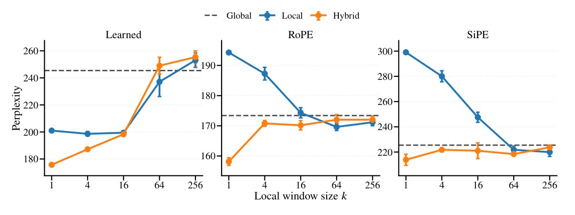
Figure 4: Perplexity on WikiText-2 for local, hybrid, and global attention patterns under different positional encodings. Curves show mean perplexity across runs for local and hybrid models as a function of the local window size , and error bars indicate standard deviations. The dashed horizontal line shows the corresponding global baseline.
图 4:不同位置编码下,局部、混合与全局注意力模式在 WikiText-2 上的困惑度。曲线给出局部与混合模型随局部窗口大小 变化的各次运行平均困惑度,误差条表示标准差。虚水平线给出相应的全局基线。
Beyond {\color[rgb]{0.4297,0.1172,0.2148}\textup{{LTL}}}\left[{\color[rgb]{0,0.4297,0.2539}\mathrel{\textup{{P}}}},{\color[rgb]{0,0.4297,0.2539}\mathrel{\textup{{Y}}}}\right].
As expected, none of the models perfectly generalizes on the two languages in {\color[rgb]{0.4297,0.1172,0.2148}\textup{{LTL}}}[{\color[rgb]{0,0.4297,0.2539}\mathrel{\textup{{S}}}}]\setminus{\color[rgb]{0.4297,0.1172,0.2148}\textup{{LTL}}}\left[{\color[rgb]{0,0.4297,0.2539}\mathrel{\textup{{P}}}},{\color[rgb]{0,0.4297,0.2539}\mathrel{\textup{{Y}}}}\right], namely the right-deterministic polynomial and bounded Dyck. Nevertheless, hybrid attention yields the strongest partial generalization on these tasks.
超出 {\color[rgb]{0.4297,0.1172,0.2148}\textup{{LTL}}}\left[{\color[rgb]{0,0.4297,0.2539}\mathrel{\textup{{P}}}},{\color[rgb]{0,0.4297,0.2539}\mathrel{\textup{{Y}}}}\right]。
正如所料,没有任何模型能够在 {\color[rgb]{0.4297,0.1172,0.2148}\textup{{LTL}}}[{\color[rgb]{0,0.4297,0.2539}\mathrel{\textup{{S}}}}]\setminus{\color[rgb]{0.4297,0.1172,0.2148}\textup{{LTL}}}\left[{\color[rgb]{0,0.4297,0.2539}\mathrel{\textup{{P}}}},{\color[rgb]{0,0.4297,0.2539}\mathrel{\textup{{Y}}}}\right] 中的两种语言上完美泛化,即右确定多项式与有界 Dyck。尽管如此,混合注意力在这些任务上给出了最强的部分泛化。
5.3.2 Positional Encodings
We now turn to the settings with positional encodings (middle and right panels of Fig. 3).
5.3.2 位置编码
我们现在转向带位置编码的设定(图 3 的中间与右侧面板)。
Global-only models.
One might hope that positional encodings would allow global attention to approximate locality. In our experiments, however, neither SiPE nor RoPE compensates for the absence of local attention: Positional encodings do not erase the qualitative separation between global-only and hybrid models; on the contrary, they often reduce performance on the tested languages.
仅全局模型。
人们或许会希望,位置编码能使全局注意力近似局部性。然而在我们的实验中,无论 SiPE 还是 RoPE,都补不上缺少局部注意力所留下的缺口:位置编码并不能抹去仅全局模型与混合模型之间的质性分离;相反,它们往往还会降低在所测语言上的表现。
Local-only and hybrid models.
With RoPE, the gap between -local and larger-window local attention becomes smaller. In particular, local-only models with or can now recognize {{{{\color[rgb]{0.0781,0.2148,0.5313}\Sigma}}^{*}}}{\color[rgb]{0.0781,0.2148,0.5313}\texttt{a}} and {{{{\color[rgb]{0.0781,0.2148,0.5313}\Sigma}}^{*}}}{\color[rgb]{0.0781,0.2148,0.5313}\texttt{a}}{\color[rgb]{0.0781,0.2148,0.5313}\texttt{b}}. In hybrid models, RoPE also enables to recognize {{{{\color[rgb]{0.0781,0.2148,0.5313}\Sigma}}^{*}}}{\color[rgb]{0.0781,0.2148,0.5313}\texttt{a}}{\color[rgb]{0.0781,0.2148,0.5313}\texttt{b}}{{{{\color[rgb]{0.0781,0.2148,0.5313}\Sigma}}^{*}}}. However, these gains come with tradeoffs, as RoPE degrades performance in several other settings. By comparison, SiPE does not narrow the gap and instead tends to reduce performance across the board.
仅局部与混合模型。
在使用 RoPE 时,-局部与更大窗口的局部注意力之间的差距会变小。特别是,仅局部模型在 或 时现在能够识别 {{{{\color[rgb]{0.0781,0.2148,0.5313}\Sigma}}^{*}}}{\color[rgb]{0.0781,0.2148,0.5313}\texttt{a}} 与 {{{{\color[rgb]{0.0781,0.2148,0.5313}\Sigma}}^{*}}}{\color[rgb]{0.0781,0.2148,0.5313}\texttt{a}}{\color[rgb]{0.0781,0.2148,0.5313}\texttt{b}}。在混合模型中,RoPE 也使 能够识别 {{{{\color[rgb]{0.0781,0.2148,0.5313}\Sigma}}^{*}}}{\color[rgb]{0.0781,0.2148,0.5313}\texttt{a}}{\color[rgb]{0.0781,0.2148,0.5313}\texttt{b}}{{{{\color[rgb]{0.0781,0.2148,0.5313}\Sigma}}^{*}}}。不过这些收益是有代价的,因为 RoPE 在若干其他设定中会损害表现。相比之下,SiPE 并没有缩小差距,反而往往全面降低表现。
Summary.
Overall, on one hand, the results under NoPE align exactly with our theory. On the other hand, the role of positional encodings is less clear-cut and merits further investigation.
小结。
总的来说,一方面,NoPE 下的结果与我们的理论完全一致。另一方面,位置编码所起的作用并不那么斩钉截铁,值得进一步考察。
6 An Experiment on Natural Language
6 一项自然语言上的实验
We also experiment with whether our theory has something to say about natural language. Thus, we run a lightweight next-token language modeling experiment on WikiText-2.
我们也实验理论是否对自然语言有所说明。因此,我们在 WikiText-2 上做了一项轻量的下一词语言建模实验。
6.1 Experimental Setup
6.1 实验设置
We train a GPT-2-small-style decoder-only Transformer from scratch, using the standard GPT-2 small architecture (12 layers, hidden size 768, 12 attention heads, and feed-forward size 3072). We keep the architecture and optimization setup fixed across all runs, varying only the attention pattern. Concretely, we compare global-only, local-only, and hybrid attention, where in the hybrid setting half of the heads are replaced by local heads. To remain consistent with the formal setup in § 3, we use strict causal masking throughout. We consider local window sizes and three positional encoding schemes: learned absolute positional embeddings, RoPE, and SiPE. For optimization, we use AdamW (Loshchilov and Hutter, 2019) with learning rate , weight decay , 2000 warmup steps, cosine learning-rate decay, per-device batch size 2, gradient accumulation of 32 steps, and early stopping based on validation loss.
我们从零训练一个 GPT-2 small 风格的仅解码器 Transformer,采用标准的 GPT-2 small 结构(12 层,隐藏维 768,12 个注意力头,前馈维 3072)。在所有运行中保持结构与优化设定不变,只改变注意力模式。具体来说,我们比较仅全局、仅局部与混合注意力,在混合设定中有一半头被换成局部头。为与第 3 节的形式设定保持一致,我们始终使用严格的因果掩码。我们考虑局部窗口大小 ,以及三种位置编码方案:学到的绝对位置嵌入、RoPE 与 SiPE。优化上使用 AdamW(Loshchilov and Hutter, 2019),学习率为 ,权重衰减为 ,预热 2000 步,余弦学习率衰减,单设备批大小为 2,梯度累积 32 步,并根据验证损失做早停。
6.2 Results
6.2 结果
The results show a clear and consistent pattern. Across all positional encoding choices, the hybrid model is always the strongest, and within the hybrid family, is always the best setting. Hybrid attention with reduces perplexity by , , relative to the global-only baseline under various positional encodings. Increasing the local window generally degrades performance, and with sufficiently large windows the hybrid model can match or underperform the global-only baseline.
结果呈现出清晰而一贯的模式。在所有位置编码选择下,混合模型始终最强,而在混合这一族里, 始终是最好的设定。窗口取 的混合注意力,相对仅全局基线,在各种位置编码下分别把困惑度降低了 、、。把局部窗口开大,一般会损害表现;窗口足够大时,混合模型可能只是打平、甚至不如仅全局基线。
We also find that local-only attention can outperform global-only attention, which is surprising but compatible with our theory, since local-only and global-only attention are incomparable in expressive power. One possible explanation is that WikiText-2 relies more heavily on short-range patterns than on the longer-range dependencies. The effect of window size, however, depends on the positional encoding. Under learned positional embeddings, smaller local windows perform better. Under RoPE and SiPE, local-only models instead tend to prefer larger windows. This is consistent with the theory: although -local attention is maximally expressive in the unbounded setting, its advantage may disappear under a fixed depth bound, especially when suitable positional encodings narrow the gap between different local window sizes.
我们还发现,仅局部注意力可以超过仅全局注意力,这虽然出人意料,却与理论相容,因为仅局部与仅全局在表达力上不可比。一种可能的解释是,WikiText-2 更依赖短程模式,而不是更长程的依赖。不过,窗口大小的影响取决于位置编码。在学到的位置嵌入下,更小的局部窗口表现更好。在 RoPE 与 SiPE 下,仅局部模型反而更偏向更大的窗口。这与理论一致:尽管 -局部注意力在无界设定下表达力最大,其优势在深度有固定上界时可能消失,尤其当合适的位置编码缩小了不同局部窗口之间的差距时。
Overall, our results support the main claim of the paper: local attention is complementary to global attention, and the hybrid setting combines the strengths of both. In particular, pairing global attention with -local attention yields the largest additional benefit.
总的来说,我们的结果支持本文的主要论断:局部注意力是对全局注意力的补充,而混合设定把二者的长处合在一起。特别是,把全局注意力与 -局部注意力配在一起,额外收益最大。
7 Conclusion
7 结论
We have given a formal account of why local attention helps in transformer language models. By connecting attention patterns to fragments of linear temporal logic, we showed that local and global attention are complementary rather than interchangeable, and that adding local attention to a globally attentive transformer strictly increases expressive power. In particular, global attention alone corresponds to the logic {\color[rgb]{0.4297,0.1172,0.2148}\textup{{LTL}}}\left[{\color[rgb]{0,0.4297,0.2539}\mathrel{\textup{{P}}}}\right], purely -local attention corresponds to {\color[rgb]{0.4297,0.1172,0.2148}\textup{{LTL}}}\left[{\color[rgb]{0,0.4297,0.2539}\mathrel{\textup{{Y}}}}^{\leq k}\right], and hybrid global–local attention corresponds to the richer logic {\color[rgb]{0.4297,0.1172,0.2148}\textup{{LTL}}}\left[{\color[rgb]{0,0.4297,0.2539}\mathrel{\textup{{P}}}},{\color[rgb]{0,0.4297,0.2539}\mathrel{\textup{{Y}}}}^{\leq k}\right]. The largest gain arises from -local attention, which induces the {\color[rgb]{0,0.4297,0.2539}\mathrel{\textup{{Y}}}} operator and captures, among other classes, the locally testable languages—a classical family beyond the reach of global-only models. Our formal-language experiments empirically confirm these separations, and a preliminary language-modeling experiment on WikiText-2 shows that hybrid attention with consistently achieves the best performance.
我们给局部注意力为何有助于 Transformer 语言模型提供了一套形式说明。通过把注意力模式与线性时序逻辑的片段联系起来,我们表明局部与全局注意力是互补的,而不是可以互换的,并且在原本使用全局注意力的 Transformer 上加入局部注意力会严格提高表达力。具体而言,单独的全局注意力对应逻辑 {\color[rgb]{0.4297,0.1172,0.2148}\textup{{LTL}}}\left[{\color[rgb]{0,0.4297,0.2539}\mathrel{\textup{{P}}}}\right],纯 -局部注意力对应 {\color[rgb]{0.4297,0.1172,0.2148}\textup{{LTL}}}\left[{\color[rgb]{0,0.4297,0.2539}\mathrel{\textup{{Y}}}}^{\leq k}\right],而全局–局部混合注意力对应更丰富的逻辑 {\color[rgb]{0.4297,0.1172,0.2148}\textup{{LTL}}}\left[{\color[rgb]{0,0.4297,0.2539}\mathrel{\textup{{P}}}},{\color[rgb]{0,0.4297,0.2539}\mathrel{\textup{{Y}}}}^{\leq k}\right]。最大的增益来自 -局部注意力,它引入 {\color[rgb]{0,0.4297,0.2539}\mathrel{\textup{{Y}}}} 算子,并且能够把握包括局部可检验语言在内的若干语言类——这是仅全局模型触及不到的一个经典家族。我们的形式语言实验从经验上确认了这些分离,而在 WikiText-2 上的初步语言建模实验表明,带 的混合注意力始终取得最好的表现。
Limitations
局限
Due to limited computational resources, we are unable to run large-scale language modeling experiments. Instead, we use a lightweight setup that is intended as a sanity check while remaining manageable in terms of model size, dataset, and training budget. Accordingly, our natural-language results should be interpreted with caution. It is possible that the qualitative picture changes with larger models, longer training, or broader datasets.
由于计算资源有限,我们无法开展大规模的语言建模实验。取而代之,我们采用一套轻量设定,意在作为合理性检查,同时在模型规模、数据与训练预算上保持可控。因此,自然语言上的结果应当谨慎解读。更大的模型、更长的训练或更广的数据,都有可能改变质性图景。
Ethical Considerations
伦理考量
We do not foresee any ethical issues.
我们预见不到伦理方面的问题。
References
参考文献
Ba et al. (2016) Jimmy Lei Ba, Jamie Ryan Kiros, and Geoffrey E. Hinton. 2016. Layer normalization . In NIPS Deep Learning Symposium .
Bahdanau et al. (2015) Dzmitry Bahdanau, Kyunghyun Cho, and Yoshua Bengio. 2015. Neural machine translation by jointly learning to align and translate . In The Third International Conference on Learning Representations .
Beltagy et al. (2020) Iz Beltagy, Matthew E. Peters, and Arman Cohan. 2020. Longformer: The long-document transformer . Computing Research Repository , arXiv:2004.05150. Version 2.
Brown et al. (2020) Tom Brown, Benjamin Mann, Nick Ryder, Melanie Subbiah, Jared D Kaplan, Prafulla Dhariwal, Arvind Neelakantan, Pranav Shyam, Girish Sastry, Amanda Askell, Sandhini Agarwal, Ariel Herbert-Voss, Gretchen Krueger, Tom Henighan, Rewon Child, Aditya Ramesh, Daniel Ziegler, Jeffrey Wu, Clemens Winter, and 12 others. 2020. Language models are few-shot learners . In Advances in Neural Information Processing Systems , volume 33, pages 1877–1901. Curran Associates, Inc.
Brzozowski et al. (2012) Janusz Brzozowski, Baiyu Li, and David Liu. 2012. Syntactic complexities of six classes of star-free languages . Journal of Automata, Languages and Combinatorics , 17(2):83–105.
Butoi et al. (2025) Alexandra Butoi, Ghazal Khalighinejad, Anej Svete, Josef Valvoda, Ryan Cotterell, and Brian DuSell. 2025. Training neural networks as recognizers of formal languages . In The Thirteenth International Conference on Learning Representations .
Chiang et al. (2023) David Chiang, Peter Cholak, and Anand Pillay. 2023. Tighter bounds on the expressivity of transformer encoders . In Proceedings of the 40th International Conference on Machine Learning , volume 202 of Proceedings of Machine Learning Research , pages 5544–5562. PMLR.
Child et al. (2019) Rewon Child, Scott Gray, Alec Radford, and Ilya Sutskever. 2019. Generating long sequences with sparse transformers . Computing Research Repository , arXiv:1904.10509.
Cohen et al. (1993) Joëlle Cohen, Dominique Perrin, and Jean-Eric Pin. 1993. On the expressive power of temporal logic . Journal of Computer and System Sciences , 46(3):271–294.
DeepSeek-AI (2025) DeepSeek-AI. 2025. DeepSeek-R1: Incentivizing reasoning capability in LLMs via reinforcement learning . Computing Research Repository , arXiv:2501.12948.
Delétang et al. (2023) Grégoire Delétang, Anian Ruoss, Jordi Grau-Moya, Tim Genewein, Li Kevin Wenliang, Elliot Catt, Chris Cundy, Marcus Hutter, Shane Legg, Joel Veness, and Pedro A Ortega. 2023. Neural networks and the chomsky hierarchy . In The Eleventh International Conference on Learning Representations .
Eilenberg (1974) Samuel Eilenberg. 1974. Automata, Languages, and Machines . Number pt. 2 in 59/B. Academic Press.
Gabbay et al. (1980) Dov Gabbay, Amir Pnueli, Saharon Shelah, and Jonathan Stavi. 1980. On the temporal analysis of fairness . POPL ’80, page 163–173, New York, NY, USA. Association for Computing Machinery.
Green (1951) James A. Green. 1951. On the structure of semigroups . Annals of Mathematics , 54(1):163–172.
Hewitt et al. (2020) John Hewitt, Michael Hahn, Surya Ganguli, Percy Liang, and Christopher D. Manning. 2020. RNNs can generate bounded hierarchical languages with optimal memory . In Proceedings of the 2020 Conference on Empirical Methods in Natural Language Processing (EMNLP) , pages 1978–2010, Online. Association for Computational Linguistics.
IEEE (2019) IEEE. 2019. IEEE standard for floating-point arithmetic . IEEE Std 754-2019.
Kamp (1968) Johan Anthony Wilem Kamp. 1968. Tense Logic and the Theory of Linear Order . Ph.D. thesis, University of California, Los Angeles.
Kingma and Ba (2014) Diederik P. Kingma and Jimmy Ba. 2014. Adam: A method for stochastic optimization . Computing Research Repository , arXiv:1412.6980. Version 9.
Kleene (1956) Stephen C. Kleene. 1956. Representation of Events in Nerve Nets and Finite Automata , pages 3–42. Princeton University Press, Princeton.
Li and Cotterell (2025) Jiaoda Li and Ryan Cotterell. 2025. Characterizing the expressivity of fixed-precision transformer language models . In The Thirty-ninth Annual Conference on Neural Information Processing Systems .
Li et al. (2024) Zhiyuan Li, Hong Liu, Denny Zhou, and Tengyu Ma. 2024. Chain of thought empowers transformers to solve inherently serial problems . In The Twelfth International Conference on Learning Representations .
Loshchilov and Hutter (2019) Ilya Loshchilov and Frank Hutter. 2019. Decoupled weight decay regularization . In The Seventh International Conference on Learning Representations .
Luong et al. (2015) Thang Luong, Hieu Pham, and Christopher D. Manning. 2015. Effective approaches to attention-based neural machine translation . In Proceedings of the 2015 Conference on Empirical Methods in Natural Language Processing , pages 1412–1421, Lisbon, Portugal. Association for Computational Linguistics.
McNaughton and Papert (1971) Robert McNaughton and Seymour Papert. 1971. Counter-free Automata . M.I.T. Press research monographs. M.I.T. Press.
Merrill and Sabharwal (2024) William Merrill and Ashish Sabharwal. 2024. The expressive power of transformers with chain of thought . In The Twelfth International Conference on Learning Representations .
OpenAI (2023) OpenAI. 2023. GPT-4 technical report . Computing Research Repository , arXiv:2303.08774.
Perles et al. (1963) Micha A. Perles, Michael O. Rabin, and Eli Shamir. 1963. The theory of definite automata . IEEE Transactions on Electronic Computers , 12:233–243.
Pnueli (1977) Amir Pnueli. 1977. The temporal logic of programs . In 18th Annual Symposium on Foundations of Computer Science (sfcs 1977) , pages 46–57.
Radford et al. (2018) Alec Radford, Karthik Narasimhan, Tim Salimans, and Ilya Sutskever. 2018. Improving language understanding by generative pre-training . OpenAI technical report.
Radford et al. (2019) Alec Radford, Jeff Wu, Rewon Child, David Luan, Dario Amodei, and Ilya Sutskever. 2019. Language models are unsupervised multitask learners . OpenAI technical report.
Schmidhuber (1992) Jürgen Schmidhuber. 1992. Learning to control fast-weight memories: An alternative to dynamic recurrent networks . In Neural Computation , volume 4, pages 131–139. MIT Press.
Straubing (1994) Howard Straubing. 1994. Finite Automata, Formal Logic, and Circuit Complexity . Progress in Theoretical Computer Science. Birkhäuser Boston, Boston, MA.
Su et al. (2024) Jianlin Su, Murtadha Ahmed, Yu Lu, Shengfeng Pan, Wen Bo, and Yunfeng Liu. 2024. Roformer: Enhanced transformer with rotary position embedding . Neurocomputing , 568:127063.
Team et al. (2025) OLMo Team, Pete Walsh, Luca Soldaini, Dirk Groeneveld, Kyle Lo, Shane Chang, Khyathi Chandu, Akshita Bhagia, Oyvind Tafjord, and 1 others. 2025. OLMo 2: The best fully open language model to date . Computing Research Repository , arXiv:2501.00656.
Vaswani et al. (2017) Ashish Vaswani, Noam Shazeer, Niki Parmar, Jakob Uszkoreit, Llion Jones, Aidan N Gomez, Łukasz Kaiser, and Illia Polosukhin. 2017. Attention is all you need . In Advances in Neural Information Processing Systems , volume 30. Curran Associates, Inc.
Wei et al. (2022) Jason Wei, Xuezhi Wang, Dale Schuurmans, Maarten Bosma, Brian Ichter, Fei Xia, Ed H Chi, Quoc V Le, and Denny Zhou. 2022. Chain-of-thought prompting elicits reasoning in large language models . In Advances in Neural Information Processing Systems , volume 35.
Wolf et al. (2020) Thomas Wolf, Lysandre Debut, Victor Sanh, Julien Chaumond, Clement Delangue, Anthony Moi, Pierric Cistac, Tim Rault, Rémi Louf, Morgan Funtowicz, Joe Davison, Sam Shleifer, Patrick von Platen, Clara Ma, Yacine Jernite, Julien Plu, Canwen Xu, Teven Le Scao, Sylvain Gugger, and 3 others. 2020. Transformers: State-of-the-art natural language processing . In Proceedings of the 2020 Conference on Empirical Methods in Natural Language Processing: System Demonstrations , pages 38–45.
Yang et al. (2025) Andy Yang, Michaël Cadilhac, and David Chiang. 2025. Knee-deep in c-RASP: A transformer depth hierarchy . In The Thirty-ninth Annual Conference on Neural Information Processing Systems .
Yang et al. (2024) Andy Yang, David Chiang, and Dana Angluin. 2024. Masked hard-attention transformers recognize exactly the star-free languages . In The Thirty-eighth Annual Conference on Neural Information Processing Systems .
Yang et al. (2026) Andy Yang, Lena Strobl, David Chiang, and Dana Angluin. 2026. Simulating hard attention using soft attention . Transactions of the Association for Computational Linguistics , 14.
Zaheer et al. (2020) Manzil Zaheer, Guru Guruganesh, Kumar Avinava Dubey, Joshua Ainslie, Chris Alberti, Santiago Ontanon, Philip Pham, Anirudh Ravula, Qifan Wang, Li Yang, and Amr Ahmed. 2020. Big bird: Transformers for longer sequences . In Advances in Neural Information Processing Systems , volume 33, pages 17283–17297. Curran Associates, Inc.
Table of Contents
目录
Appendix A Linear Temporal Logic
附录 A 线性时序逻辑
We now give the basic definitions of linear temporal logic.
下面给出线性时序逻辑的基本定义。
A.1 Syntax
A.1 语法
We define the syntax of full linear temporal logic, {\color[rgb]{0.4297,0.1172,0.2148}\textup{{LTL}}}[{\color[rgb]{0,0.4297,0.2539}\mathrel{\textup{{P}}}},{\color[rgb]{0,0.4297,0.2539}\mathrel{\textup{{Y}}}},{\color[rgb]{0,0.4297,0.2539}\mathrel{\textup{{S}}}},{\color[rgb]{0,0.4297,0.2539}\mathrel{\textup{{U}}}}], over an alphabet {{\color[rgb]{0.0781,0.2148,0.5313}\Sigma}}. The set of formulas over {{\color[rgb]{0.0781,0.2148,0.5313}\Sigma}} is defined inductively:
我们在字母表 {{\color[rgb]{0.0781,0.2148,0.5313}\Sigma}} 上定义完整线性时序逻辑 {\color[rgb]{0.4297,0.1172,0.2148}\textup{{LTL}}}[{\color[rgb]{0,0.4297,0.2539}\mathrel{\textup{{P}}}},{\color[rgb]{0,0.4297,0.2539}\mathrel{\textup{{Y}}}},{\color[rgb]{0,0.4297,0.2539}\mathrel{\textup{{S}}}},{\color[rgb]{0,0.4297,0.2539}\mathrel{\textup{{U}}}}] 的语法。{{\color[rgb]{0.0781,0.2148,0.5313}\Sigma}} 上的公式集合按归纳定义如下:
- • Constants: and are formulas.
- • 常数: 与 是公式。
- • Atomic predicates: {\color[rgb]{0.6875,0.2734,0.1172}\pi}_{\color[rgb]{0.0781,0.2148,0.5313}\texttt{a}} is a formula for {\color[rgb]{0.0781,0.2148,0.5313}\texttt{a}}\in{{\color[rgb]{0.0781,0.2148,0.5313}\Sigma}}.
- • 原子谓词: 对 {\color[rgb]{0.0781,0.2148,0.5313}\texttt{a}}\in{{\color[rgb]{0.0781,0.2148,0.5313}\Sigma}},{\color[rgb]{0.6875,0.2734,0.1172}\pi}_{\color[rgb]{0.0781,0.2148,0.5313}\texttt{a}} 是公式。
- • Boolean connectives: if {\color[rgb]{0.6875,0.2734,0.1172}\psi}_{1} and {\color[rgb]{0.6875,0.2734,0.1172}\psi}_{2} are formulas, then so are \lnot{\color[rgb]{0.6875,0.2734,0.1172}\psi}_{1}, {\color[rgb]{0.6875,0.2734,0.1172}\psi}_{1}\land{\color[rgb]{0.6875,0.2734,0.1172}\psi}_{2}, and {\color[rgb]{0.6875,0.2734,0.1172}\psi}_{1}\lor{\color[rgb]{0.6875,0.2734,0.1172}\psi}_{2}.
- • 布尔联结词: 若 {\color[rgb]{0.6875,0.2734,0.1172}\psi}_{1} 与 {\color[rgb]{0.6875,0.2734,0.1172}\psi}_{2} 是公式,则 \lnot{\color[rgb]{0.6875,0.2734,0.1172}\psi}_{1}、{\color[rgb]{0.6875,0.2734,0.1172}\psi}_{1}\land{\color[rgb]{0.6875,0.2734,0.1172}\psi}_{2} 与 {\color[rgb]{0.6875,0.2734,0.1172}\psi}_{1}\lor{\color[rgb]{0.6875,0.2734,0.1172}\psi}_{2} 也是公式。
- • Temporal operators: if {\color[rgb]{0.6875,0.2734,0.1172}\psi} and {\color[rgb]{0.6875,0.2734,0.1172}\psi}^{\prime} are formulas, then so are {\color[rgb]{0,0.4297,0.2539}\mathrel{\textup{{Y}}}}{\color[rgb]{0.6875,0.2734,0.1172}\psi} (“yesterday”), {\color[rgb]{0,0.4297,0.2539}\mathrel{\textup{{P}}}}{\color[rgb]{0.6875,0.2734,0.1172}\psi} (“past”), {\color[rgb]{0.6875,0.2734,0.1172}\psi}{\color[rgb]{0,0.4297,0.2539}\mathrel{\textup{{S}}}}{\color[rgb]{0.6875,0.2734,0.1172}\psi}^{\prime} (“since”), and {\color[rgb]{0.6875,0.2734,0.1172}\psi}{\color[rgb]{0,0.4297,0.2539}\mathrel{\textup{{U}}}}{\color[rgb]{0.6875,0.2734,0.1172}\psi}^{\prime} (“until”).
- • 时序算子: 若 {\color[rgb]{0.6875,0.2734,0.1172}\psi} 与 {\color[rgb]{0.6875,0.2734,0.1172}\psi}^{\prime} 是公式,则 {\color[rgb]{0,0.4297,0.2539}\mathrel{\textup{{Y}}}}{\color[rgb]{0.6875,0.2734,0.1172}\psi}(“昨天”)、{\color[rgb]{0,0.4297,0.2539}\mathrel{\textup{{P}}}}{\color[rgb]{0.6875,0.2734,0.1172}\psi}(“过去”)、{\color[rgb]{0.6875,0.2734,0.1172}\psi}{\color[rgb]{0,0.4297,0.2539}\mathrel{\textup{{S}}}}{\color[rgb]{0.6875,0.2734,0.1172}\psi}^{\prime}(“自从”)以及 {\color[rgb]{0.6875,0.2734,0.1172}\psi}{\color[rgb]{0,0.4297,0.2539}\mathrel{\textup{{U}}}}{\color[rgb]{0.6875,0.2734,0.1172}\psi}^{\prime}(“直到”)也是公式。
A.2 Operator Depth
A.2 算子深度
The operator depth of a formula {\color[rgb]{0.6875,0.2734,0.1172}\phi}, denoted {\text{od}}({\color[rgb]{0.6875,0.2734,0.1172}\phi}), is defined inductively:
公式 {\color[rgb]{0.6875,0.2734,0.1172}\phi} 的算子深度记作 {\text{od}}({\color[rgb]{0.6875,0.2734,0.1172}\phi}),按归纳定义如下:
$${\text{od}}({\color[rgb]{0.6875,0.2734,0.1172}\phi})\mathrel{\stackrel{{\scriptstyle\textnormal{def}}}{{=}}}\begin{cases}0&\text{if }{\color[rgb]{0.6875,0.2734,0.1172}\phi}\in{{\top},,{\bot},,{\color[rgb]{0.6875,0.2734,0.1172}\pi}{\color[rgb]{0.0781,0.2148,0.5313}\texttt{a}}}\[3.0pt]
{\text{od}}({\color[rgb]{0.6875,0.2734,0.1172}\psi})&\text{if }{\color[rgb]{0.6875,0.2734,0.1172}\phi}=\lnot{\color[rgb]{0.6875,0.2734,0.1172}\psi}\[3.0pt]
\max\big({\text{od}}({\color[rgb]{0.6875,0.2734,0.1172}\psi}{1}),,{\text{od}}({\color[rgb]{0.6875,0.2734,0.1172}\psi}{2})\big)&\text{if }{\color[rgb]{0.6875,0.2734,0.1172}\phi}={\color[rgb]{0.6875,0.2734,0.1172}\psi}{1}\circ{\color[rgb]{0.6875,0.2734,0.1172}\psi}{2},;\circ\in{\land,\lor}\[3.0pt]
1+{\text{od}}({\color[rgb]{0.6875,0.2734,0.1172}\psi})&\text{if }{\color[rgb]{0.6875,0.2734,0.1172}\phi}=\circ,{\color[rgb]{0.6875,0.2734,0.1172}\psi},;\circ\in{{\color[rgb]{0,0.4297,0.2539}\mathrel{\textup{{Y}}}},{\color[rgb]{0,0.4297,0.2539}\mathrel{\textup{{P}}}}}\[3.0pt]
1+\max\big({\text{od}}({\color[rgb]{0.6875,0.2734,0.1172}\psi}{1}),,{\text{od}}({\color[rgb]{0.6875,0.2734,0.1172}\psi}{2})\big)&\text{if }{\color[rgb]{0.6875,0.2734,0.1172}\phi}={\color[rgb]{0.6875,0.2734,0.1172}\psi}{1}\circ{\color[rgb]{0.6875,0.2734,0.1172}\psi}_{2},;\circ\in{{\color[rgb]{0,0.4297,0.2539}\mathrel{\textup{{S}}}},{\color[rgb]{0,0.4297,0.2539}\mathrel{\textup{{U}}}}}\end{cases} \tag{15}$$
A.3 Semantics
A.3 语义
Given a string w and a position , the semantics for the satisfaction relation {{\color[rgb]{0.0781,0.2148,0.5313}\textbf{{w}}}},n\models{\color[rgb]{0.6875,0.2734,0.1172}\psi} is defined as:
给定字符串 w 与位置 ,满足关系 {{\color[rgb]{0.0781,0.2148,0.5313}\textbf{{w}}}},n\models{\color[rgb]{0.6875,0.2734,0.1172}\psi} 的语义定义如下:
- • {{\color[rgb]{0.0781,0.2148,0.5313}\textbf{{w}}}},n\models{\color[rgb]{0.6875,0.2734,0.1172}\pi}_{\color[rgb]{0.0781,0.2148,0.5313}\texttt{a}} iff 1\leq n\leq|{{\color[rgb]{0.0781,0.2148,0.5313}\textbf{{w}}}}| and the token of w is a;
- • {{\color[rgb]{0.0781,0.2148,0.5313}\textbf{{w}}}},n\models{\color[rgb]{0.6875,0.2734,0.1172}\pi}_{\color[rgb]{0.0781,0.2148,0.5313}\texttt{a}} 当且仅当 1\leq n\leq|{{\color[rgb]{0.0781,0.2148,0.5313}\textbf{{w}}}}| 且 w 的第 个词元是 a;
- • {{\color[rgb]{0.0781,0.2148,0.5313}\textbf{{w}}}},n\models{\color[rgb]{0.6875,0.2734,0.1172}\psi}_{1}\lor{\color[rgb]{0.6875,0.2734,0.1172}\psi}_{2} iff {{\color[rgb]{0.0781,0.2148,0.5313}\textbf{{w}}}},n\models{\color[rgb]{0.6875,0.2734,0.1172}\psi}_{1} or {{\color[rgb]{0.0781,0.2148,0.5313}\textbf{{w}}}},n\models{\color[rgb]{0.6875,0.2734,0.1172}\psi}_{2};
- • {{\color[rgb]{0.0781,0.2148,0.5313}\textbf{{w}}}},n\models{\color[rgb]{0.6875,0.2734,0.1172}\psi}_{1}\lor{\color[rgb]{0.6875,0.2734,0.1172}\psi}_{2} 当且仅当 {{\color[rgb]{0.0781,0.2148,0.5313}\textbf{{w}}}},n\models{\color[rgb]{0.6875,0.2734,0.1172}\psi}_{1} 或 {{\color[rgb]{0.0781,0.2148,0.5313}\textbf{{w}}}},n\models{\color[rgb]{0.6875,0.2734,0.1172}\psi}_{2};
- • {{\color[rgb]{0.0781,0.2148,0.5313}\textbf{{w}}}},n\models{\color[rgb]{0.6875,0.2734,0.1172}\psi}_{1}\land{\color[rgb]{0.6875,0.2734,0.1172}\psi}_{2} iff {{\color[rgb]{0.0781,0.2148,0.5313}\textbf{{w}}}},n\models{\color[rgb]{0.6875,0.2734,0.1172}\psi}_{1} and {{\color[rgb]{0.0781,0.2148,0.5313}\textbf{{w}}}},n\models{\color[rgb]{0.6875,0.2734,0.1172}\psi}_{2};
- • {{\color[rgb]{0.0781,0.2148,0.5313}\textbf{{w}}}},n\models{\color[rgb]{0.6875,0.2734,0.1172}\psi}_{1}\land{\color[rgb]{0.6875,0.2734,0.1172}\psi}_{2} 当且仅当 {{\color[rgb]{0.0781,0.2148,0.5313}\textbf{{w}}}},n\models{\color[rgb]{0.6875,0.2734,0.1172}\psi}_{1} 且 {{\color[rgb]{0.0781,0.2148,0.5313}\textbf{{w}}}},n\models{\color[rgb]{0.6875,0.2734,0.1172}\psi}_{2};
- • {{\color[rgb]{0.0781,0.2148,0.5313}\textbf{{w}}}},n\models\lnot{\color[rgb]{0.6875,0.2734,0.1172}\psi} iff {{\color[rgb]{0.0781,0.2148,0.5313}\textbf{{w}}}},n\not\models{\color[rgb]{0.6875,0.2734,0.1172}\psi};
- • {{\color[rgb]{0.0781,0.2148,0.5313}\textbf{{w}}}},n\models\lnot{\color[rgb]{0.6875,0.2734,0.1172}\psi} 当且仅当 {{\color[rgb]{0.0781,0.2148,0.5313}\textbf{{w}}}},n\not\models{\color[rgb]{0.6875,0.2734,0.1172}\psi};
- • {{\color[rgb]{0.0781,0.2148,0.5313}\textbf{{w}}}},n\models{\color[rgb]{0,0.4297,0.2539}\mathrel{\textup{{Y}}}}{\color[rgb]{0.6875,0.2734,0.1172}\psi} iff {{\color[rgb]{0.0781,0.2148,0.5313}\textbf{{w}}}},n-1\models{\color[rgb]{0.6875,0.2734,0.1172}\psi};
- • {{\color[rgb]{0.0781,0.2148,0.5313}\textbf{{w}}}},n\models{\color[rgb]{0,0.4297,0.2539}\mathrel{\textup{{Y}}}}{\color[rgb]{0.6875,0.2734,0.1172}\psi} 当且仅当 {{\color[rgb]{0.0781,0.2148,0.5313}\textbf{{w}}}},n-1\models{\color[rgb]{0.6875,0.2734,0.1172}\psi};
- • {{\color[rgb]{0.0781,0.2148,0.5313}\textbf{{w}}}},n\models{\color[rgb]{0,0.4297,0.2539}\mathrel{\textup{{P}}}}{\color[rgb]{0.6875,0.2734,0.1172}\psi} iff there exists such that and {{\color[rgb]{0.0781,0.2148,0.5313}\textbf{{w}}}},m\models{\color[rgb]{0.6875,0.2734,0.1172}\psi};
- • {{\color[rgb]{0.0781,0.2148,0.5313}\textbf{{w}}}},n\models{\color[rgb]{0,0.4297,0.2539}\mathrel{\textup{{P}}}}{\color[rgb]{0.6875,0.2734,0.1172}\psi} 当且仅当存在 使得 且 {{\color[rgb]{0.0781,0.2148,0.5313}\textbf{{w}}}},m\models{\color[rgb]{0.6875,0.2734,0.1172}\psi};
- • {{\color[rgb]{0.0781,0.2148,0.5313}\textbf{{w}}}},n\models{\color[rgb]{0.6875,0.2734,0.1172}\psi}_{1}{\color[rgb]{0,0.4297,0.2539}\mathrel{\textup{{S}}}}{\color[rgb]{0.6875,0.2734,0.1172}\psi}_{2} iff there exists such that , {{\color[rgb]{0.0781,0.2148,0.5313}\textbf{{w}}}},m\models{\color[rgb]{0.6875,0.2734,0.1172}\psi}_{2}, and for all such that , {{\color[rgb]{0.0781,0.2148,0.5313}\textbf{{w}}}},i\models{\color[rgb]{0.6875,0.2734,0.1172}\psi}_{1};
- • {{\color[rgb]{0.0781,0.2148,0.5313}\textbf{{w}}}},n\models{\color[rgb]{0.6875,0.2734,0.1172}\psi}_{1}{\color[rgb]{0,0.4297,0.2539}\mathrel{\textup{{S}}}}{\color[rgb]{0.6875,0.2734,0.1172}\psi}_{2} 当且仅当存在 使得 ,{{\color[rgb]{0.0781,0.2148,0.5313}\textbf{{w}}}},m\models{\color[rgb]{0.6875,0.2734,0.1172}\psi}_{2},并且对所有满足 的 ,有 {{\color[rgb]{0.0781,0.2148,0.5313}\textbf{{w}}}},i\models{\color[rgb]{0.6875,0.2734,0.1172}\psi}_{1};
- • {{\color[rgb]{0.0781,0.2148,0.5313}\textbf{{w}}}},n\models{\color[rgb]{0.6875,0.2734,0.1172}\psi}_{1}{\color[rgb]{0,0.4297,0.2539}\mathrel{\textup{{U}}}}{\color[rgb]{0.6875,0.2734,0.1172}\psi}_{2} iff there exists such that , {{\color[rgb]{0.0781,0.2148,0.5313}\textbf{{w}}}},m\models{\color[rgb]{0.6875,0.2734,0.1172}\psi}_{2}, and for all such that , {{\color[rgb]{0.0781,0.2148,0.5313}\textbf{{w}}}},i\models{\color[rgb]{0.6875,0.2734,0.1172}\psi}_{1}.
- • {{\color[rgb]{0.0781,0.2148,0.5313}\textbf{{w}}}},n\models{\color[rgb]{0.6875,0.2734,0.1172}\psi}_{1}{\color[rgb]{0,0.4297,0.2539}\mathrel{\textup{{U}}}}{\color[rgb]{0.6875,0.2734,0.1172}\psi}_{2} 当且仅当存在 使得 ,{{\color[rgb]{0.0781,0.2148,0.5313}\textbf{{w}}}},m\models{\color[rgb]{0.6875,0.2734,0.1172}\psi}_{2},并且对所有满足 的 ,有 {{\color[rgb]{0.0781,0.2148,0.5313}\textbf{{w}}}},i\models{\color[rgb]{0.6875,0.2734,0.1172}\psi}_{1}。
A string w of length satisfies a formula {\color[rgb]{0.6875,0.2734,0.1172}\psi}, written {{\color[rgb]{0.0781,0.2148,0.5313}\textbf{{w}}}}\models{\color[rgb]{0.6875,0.2734,0.1172}\psi}, if {\color[rgb]{0.6875,0.2734,0.1172}\psi} holds at a position outside the string, such as position or . In this work, we evaluate formulas at position , just beyond the end of the string, since we consider only past-time operators such as {\color[rgb]{0,0.4297,0.2539}\mathrel{\textup{{Y}}}} and {\color[rgb]{0,0.4297,0.2539}\mathrel{\textup{{P}}}}, i.e.,
长度为 的字符串 w 满足公式 {\color[rgb]{0.6875,0.2734,0.1172}\psi},记作 {{\color[rgb]{0.0781,0.2148,0.5313}\textbf{{w}}}}\models{\color[rgb]{0.6875,0.2734,0.1172}\psi},若 {\color[rgb]{0.6875,0.2734,0.1172}\psi} 在字符串之外的某个位置成立,例如位置 或 。本工作中,我们在位置 处、也就是字符串末尾刚刚之后求值公式,因为我们只考虑 {\color[rgb]{0,0.4297,0.2539}\mathrel{\textup{{Y}}}} 与 {\color[rgb]{0,0.4297,0.2539}\mathrel{\textup{{P}}}} 这类过去时算子,即
{{\color[rgb]{0.0781,0.2148,0.5313}\textbf{{w}}}}\models{\color[rgb]{0.6875,0.2734,0.1172}\psi}\quad\text{iff}\quad{{\color[rgb]{0.0781,0.2148,0.5313}\textbf{{w}}}},N+1\models{\color[rgb]{0.6875,0.2734,0.1172}\psi}. \tag{16}
The language defined by a formula {\color[rgb]{0.6875,0.2734,0.1172}\psi} is the set of all strings that satisfy it, i.e., the set
由公式 {\color[rgb]{0.6875,0.2734,0.1172}\psi} 定义的语言,是满足它的全部字符串之集,也就是集合
{{\color[rgb]{0.0781,0.2148,0.5313}\mathbb{L}}}({\color[rgb]{0.6875,0.2734,0.1172}\psi})\mathrel{\stackrel{{\scriptstyle\textnormal{def}}}{{=}}}\{{{\color[rgb]{0.0781,0.2148,0.5313}\textbf{{w}}}}\in{{{{\color[rgb]{0.0781,0.2148,0.5313}\Sigma}}^{*}}}\mid{{\color[rgb]{0.0781,0.2148,0.5313}\textbf{{w}}}}\models{\color[rgb]{0.6875,0.2734,0.1172}\psi}\}. \tag{17}
Appendix B Additional Background
附录 B 补充背景
We collect background on formal language classes, syntactic semigroups, and deterministic finite automata, which we use to characterize transformers under different attention patterns.
我们汇集关于形式语言类、句法半群以及确定有限自动机的背景,用以刻画不同注意力模式之下的 Transformer。
B.1 Formal Languages
B.1 形式语言
Regular Languages.
A regular expression is a declarative description of a language over {{\color[rgb]{0.0781,0.2148,0.5313}\Sigma}}. It is defined inductively as follows:
正则语言。
正则表达式是对 {{\color[rgb]{0.0781,0.2148,0.5313}\Sigma}} 上某个语言的陈述性描述。它按归纳定义如下:
- • and each {\color[rgb]{0.0781,0.2148,0.5313}\texttt{a}}\in{{\color[rgb]{0.0781,0.2148,0.5313}\Sigma}} are regular expressions;
- • 以及每个 {\color[rgb]{0.0781,0.2148,0.5313}\texttt{a}}\in{{\color[rgb]{0.0781,0.2148,0.5313}\Sigma}} 都是正则表达式;
- • if and are regular expressions, then so are the union , the concatenation , the Kleene star , and the complement .
- • 若 与 是正则表达式,则并 、连接 、Kleene 星 以及补 也是正则表达式。
A language is regular if and only if it can be described by a regular expression (Kleene, 1956). A regular language is star-free if it can be described by a regular expression that does not use the Kleene star (McNaughton and Papert, 1971). For example, {{{{\color[rgb]{0.0781,0.2148,0.5313}\Sigma}}^{*}}} is star-free, since it can be described by the regular expression .
一个语言是正则的,当且仅当它可以被某个正则表达式描述(Kleene, 1956)。一个正则语言是无星的,若它可以被不含 Kleene 星的正则表达式描述(McNaughton and Papert, 1971)。例如 {{{{\color[rgb]{0.0781,0.2148,0.5313}\Sigma}}^{*}}} 是无星的,因为它可以被正则表达式 描述。
Monomials.
A monomial over {{\color[rgb]{0.0781,0.2148,0.5313}\Sigma}} is a language of the form {{\color[rgb]{0.0781,0.2148,0.5313}\Sigma}}_{0}^{*}{\color[rgb]{0.0781,0.2148,0.5313}\texttt{a}}_{1}{{\color[rgb]{0.0781,0.2148,0.5313}\Sigma}}_{1}^{*}\cdots{\color[rgb]{0.0781,0.2148,0.5313}\texttt{a}}_{n}{{\color[rgb]{0.0781,0.2148,0.5313}\Sigma}}_{n}^{*}, where {\color[rgb]{0.0781,0.2148,0.5313}\texttt{a}}_{1},\ldots,{\color[rgb]{0.0781,0.2148,0.5313}\texttt{a}}_{n}\in{{\color[rgb]{0.0781,0.2148,0.5313}\Sigma}} and {{\color[rgb]{0.0781,0.2148,0.5313}\Sigma}}_{0},{{\color[rgb]{0.0781,0.2148,0.5313}\Sigma}}_{1},\ldots,{{\color[rgb]{0.0781,0.2148,0.5313}\Sigma}}_{n}\subseteq{{\color[rgb]{0.0781,0.2148,0.5313}\Sigma}}. A monomial is called
单项式。
{{\color[rgb]{0.0781,0.2148,0.5313}\Sigma}} 上的单项式是形如 {{\color[rgb]{0.0781,0.2148,0.5313}\Sigma}}_{0}^{*}{\color[rgb]{0.0781,0.2148,0.5313}\texttt{a}}_{1}{{\color[rgb]{0.0781,0.2148,0.5313}\Sigma}}_{1}^{*}\cdots{\color[rgb]{0.0781,0.2148,0.5313}\texttt{a}}_{n}{{\color[rgb]{0.0781,0.2148,0.5313}\Sigma}}_{n}^{*} 的语言,其中 {\color[rgb]{0.0781,0.2148,0.5313}\texttt{a}}_{1},\ldots,{\color[rgb]{0.0781,0.2148,0.5313}\texttt{a}}_{n}\in{{\color[rgb]{0.0781,0.2148,0.5313}\Sigma}} 且 {{\color[rgb]{0.0781,0.2148,0.5313}\Sigma}}_{0},{{\color[rgb]{0.0781,0.2148,0.5313}\Sigma}}_{1},\ldots,{{\color[rgb]{0.0781,0.2148,0.5313}\Sigma}}_{n}\subseteq{{\color[rgb]{0.0781,0.2148,0.5313}\Sigma}}。一个单项式称为
- • left-deterministic if for every , {\color[rgb]{0.0781,0.2148,0.5313}\texttt{a}}_{k}\notin{{\color[rgb]{0.0781,0.2148,0.5313}\Sigma}}_{k-1};
- • 左确定的,若对每个 ,有 {\color[rgb]{0.0781,0.2148,0.5313}\texttt{a}}_{k}\notin{{\color[rgb]{0.0781,0.2148,0.5313}\Sigma}}_{k-1};
- • right-deterministic if for every , {\color[rgb]{0.0781,0.2148,0.5313}\texttt{a}}_{k}\notin{{\color[rgb]{0.0781,0.2148,0.5313}\Sigma}}_{k};
- • 右确定的,若对每个 ,有 {\color[rgb]{0.0781,0.2148,0.5313}\texttt{a}}_{k}\notin{{\color[rgb]{0.0781,0.2148,0.5313}\Sigma}}_{k};
- • unambiguous if every string w in the monomial admits at most one factorization {{\color[rgb]{0.0781,0.2148,0.5313}\textbf{{w}}}}={{\color[rgb]{0.0781,0.2148,0.5313}\textbf{{w}}}}_{0}{\color[rgb]{0.0781,0.2148,0.5313}\texttt{a}}_{1}{{\color[rgb]{0.0781,0.2148,0.5313}\textbf{{w}}}}_{1}\cdots{\color[rgb]{0.0781,0.2148,0.5313}\texttt{a}}_{n}{{\color[rgb]{0.0781,0.2148,0.5313}\textbf{{w}}}}_{n} with {{\color[rgb]{0.0781,0.2148,0.5313}\textbf{{w}}}}_{k}\in{{{{\color[rgb]{0.0781,0.2148,0.5313}\Sigma}}_{k}^{*}}} for all .
- • 无歧义的,若该单项式中的每个字符串 w 至多允许一种分解 {{\color[rgb]{0.0781,0.2148,0.5313}\textbf{{w}}}}={{\color[rgb]{0.0781,0.2148,0.5313}\textbf{{w}}}}_{0}{\color[rgb]{0.0781,0.2148,0.5313}\texttt{a}}_{1}{{\color[rgb]{0.0781,0.2148,0.5313}\textbf{{w}}}}_{1}\cdots{\color[rgb]{0.0781,0.2148,0.5313}\texttt{a}}_{n}{{\color[rgb]{0.0781,0.2148,0.5313}\textbf{{w}}}}_{n},使得对所有 有 {{\color[rgb]{0.0781,0.2148,0.5313}\textbf{{w}}}}_{k}\in{{{{\color[rgb]{0.0781,0.2148,0.5313}\Sigma}}_{k}^{*}}}。
Polynomials.
A polynomial is a finite union of monomials. It is called left-deterministic (resp. right-deterministic or unambiguous) if it is a finite disjoint union of left-deterministic (resp. right-deterministic or unambiguous) monomials.
多项式。
多项式是有限多个单项式的并。若它是有限多个互不相交的左确定(分别地,右确定或无歧义)单项式的并,则称它是左确定的(分别地,右确定的或无歧义的)。
B.2 Syntactic Monoids and Semigroups
B.2 句法幺半群与半群
Semigroups and Monoids.
A semigroup is a set endowed with an associative binary operation. A monoid is a semigroup with an identity element.
半群与幺半群。
半群是配备了结合的二元运算的集合。幺半群是带单位元的半群。
-trivial Monoids.
Recall Green’s relation on a monoid {\color[rgb]{0.5586,0.4023,0.0742}\mathbb{M}} (Green, 1951). For s,t\in{\color[rgb]{0.5586,0.4023,0.0742}\mathbb{M}}, we write if they generate the same principal right ideal:
-平凡幺半群。
回顾幺半群 {\color[rgb]{0.5586,0.4023,0.0742}\mathbb{M}} 上 Green 的 关系(Green, 1951)。对 s,t\in{\color[rgb]{0.5586,0.4023,0.0742}\mathbb{M}},若它们生成同一个主右理想,则记 :
s{\color[rgb]{0.5586,0.4023,0.0742}\mathbb{M}}=t{\color[rgb]{0.5586,0.4023,0.0742}\mathbb{M}}. \tag{18}
A monoid {\color[rgb]{0.5586,0.4023,0.0742}\mathbb{M}} is -trivial if is equality; equivalently, for all s,t\in{\color[rgb]{0.5586,0.4023,0.0742}\mathbb{M}},
幺半群 {\color[rgb]{0.5586,0.4023,0.0742}\mathbb{M}} 是 -平凡的,若 就是相等关系;等价地,对所有 s,t\in{\color[rgb]{0.5586,0.4023,0.0742}\mathbb{M}},
Locally -trivial Semigroups.
An element {e}\in{\color[rgb]{0.5586,0.4023,0.0742}\mathbb{S}} is idempotent if . A semigroup {\color[rgb]{0.5586,0.4023,0.0742}\mathbb{S}} is locally -trivial if, for every idempotent {e}\in{\color[rgb]{0.5586,0.4023,0.0742}\mathbb{S}}, the submonoid
局部 -平凡半群。
元素 {e}\in{\color[rgb]{0.5586,0.4023,0.0742}\mathbb{S}} 是幂等元,若 。半群 {\color[rgb]{0.5586,0.4023,0.0742}\mathbb{S}} 是局部 -平凡的,若对每个幂等元 {e}\in{\color[rgb]{0.5586,0.4023,0.0742}\mathbb{S}},子幺半群
{e}{\color[rgb]{0.5586,0.4023,0.0742}\mathbb{S}}{e}\mathrel{\stackrel{{\scriptstyle\textnormal{def}}}{{=}}}\{{e}s{e}\mid s\in{\color[rgb]{0.5586,0.4023,0.0742}\mathbb{S}}\} \tag{20}
with identity element is -trivial.
以 为单位元,是 -平凡的。
Syntactic Congruence.
Let {{\color[rgb]{0.0781,0.2148,0.5313}L}}\subseteq{{{{\color[rgb]{0.0781,0.2148,0.5313}\Sigma}}^{*}}} be a language. Two strings {{\color[rgb]{0.0781,0.2148,0.5313}\textbf{{s}}}},{{\color[rgb]{0.0781,0.2148,0.5313}\textbf{{t}}}}\in{{{{\color[rgb]{0.0781,0.2148,0.5313}\Sigma}}^{*}}} are syntactically equivalent, denoted {{\color[rgb]{0.0781,0.2148,0.5313}\textbf{{s}}}}{\equiv_{{\color[rgb]{0.0781,0.2148,0.5313}L}}}{{\color[rgb]{0.0781,0.2148,0.5313}\textbf{{t}}}}, if
句法同余。
设 {{\color[rgb]{0.0781,0.2148,0.5313}L}}\subseteq{{{{\color[rgb]{0.0781,0.2148,0.5313}\Sigma}}^{*}}} 为一个语言。两个字符串 {{\color[rgb]{0.0781,0.2148,0.5313}\textbf{{s}}}},{{\color[rgb]{0.0781,0.2148,0.5313}\textbf{{t}}}}\in{{{{\color[rgb]{0.0781,0.2148,0.5313}\Sigma}}^{*}}} 是句法等价的,记作 {{\color[rgb]{0.0781,0.2148,0.5313}\textbf{{s}}}}{\equiv_{{\color[rgb]{0.0781,0.2148,0.5313}L}}}{{\color[rgb]{0.0781,0.2148,0.5313}\textbf{{t}}}},若
\forall\,{{\color[rgb]{0.0781,0.2148,0.5313}\textbf{{u}}}},{{\color[rgb]{0.0781,0.2148,0.5313}\textbf{{v}}}}\in{{{{\color[rgb]{0.0781,0.2148,0.5313}\Sigma}}^{*}}}\colon\qquad{{\color[rgb]{0.0781,0.2148,0.5313}\textbf{{u}}}}{{\color[rgb]{0.0781,0.2148,0.5313}\textbf{{s}}}}{{\color[rgb]{0.0781,0.2148,0.5313}\textbf{{v}}}}\in{{\color[rgb]{0.0781,0.2148,0.5313}L}}\ \Leftrightarrow\ {{\color[rgb]{0.0781,0.2148,0.5313}\textbf{{u}}}}{{\color[rgb]{0.0781,0.2148,0.5313}\textbf{{t}}}}{{\color[rgb]{0.0781,0.2148,0.5313}\textbf{{v}}}}\in{{\color[rgb]{0.0781,0.2148,0.5313}L}}. \tag{21}
We write {{\left[{{\color[rgb]{0.0781,0.2148,0.5313}\textbf{{w}}}}\right]}} for the equivalence class of w.
我们把 w 的等价类记作 {{\left[{{\color[rgb]{0.0781,0.2148,0.5313}\textbf{{w}}}}\right]}}。
Syntactic Monoid.
The quotient monoid
句法幺半群。
商幺半群
{{{{\color[rgb]{0.0781,0.2148,0.5313}\Sigma}}^{*}}}/{\equiv_{{\color[rgb]{0.0781,0.2148,0.5313}L}}}, \tag{22}
whose elements are equivalence classes and whose operation is induced by concatenation, is called the syntactic monoid of {{\color[rgb]{0.0781,0.2148,0.5313}L}}.
其元素为等价类、运算由连接诱导,称为 {{\color[rgb]{0.0781,0.2148,0.5313}L}} 的句法幺半群。
Syntactic Semigroup.
Let {{\color[rgb]{0.0781,0.2148,0.5313}\Sigma}}^{+} denote the set of nonempty strings over {{\color[rgb]{0.0781,0.2148,0.5313}\Sigma}}. Restricting the syntactic congruence to {{\color[rgb]{0.0781,0.2148,0.5313}\Sigma}}^{+} yields the quotient semigroup
句法半群。
设 {{\color[rgb]{0.0781,0.2148,0.5313}\Sigma}}^{+} 表示 {{\color[rgb]{0.0781,0.2148,0.5313}\Sigma}} 上非空字符串之集。把句法同余限制到 {{\color[rgb]{0.0781,0.2148,0.5313}\Sigma}}^{+} 上,得到商半群
{{\color[rgb]{0.0781,0.2148,0.5313}\Sigma}}^{+}/{\equiv_{{\color[rgb]{0.0781,0.2148,0.5313}L}}}. \tag{23}
This quotient is called the syntactic semigroup of {{\color[rgb]{0.0781,0.2148,0.5313}L}}.
这一商称为 {{\color[rgb]{0.0781,0.2148,0.5313}L}} 的句法半群。
B.3 Deterministic Finite Automata
B.3 确定有限自动机
Definition.
A deterministic finite automaton (DFA) is a -tuple {{\color[rgb]{0.5586,0.4023,0.0742}\mathcal{A}}}={{\left({{\color[rgb]{0.0781,0.2148,0.5313}\Sigma}},{{Q}},{{q_{{{I}}}}},{{F}},{{\delta}}\right)}}, where
定义。
确定有限自动机(DFA)是一个五元组 {{\color[rgb]{0.5586,0.4023,0.0742}\mathcal{A}}}={{\left({{\color[rgb]{0.0781,0.2148,0.5313}\Sigma}},{{Q}},{{q_{{{I}}}}},{{F}},{{\delta}}\right)}},其中
- • {{\color[rgb]{0.0781,0.2148,0.5313}\Sigma}} is an alphabet;
- • {{\color[rgb]{0.0781,0.2148,0.5313}\Sigma}} 是一个字母表;
- • is a finite set of states;
- • 是有限的状态集;
- • is the initial state;
- • 是初始状态;
- • is the set of accepting states;
- • 是接受状态之集;
- • {{\delta}}\colon{{Q}}\times{{\color[rgb]{0.0781,0.2148,0.5313}\Sigma}}\to{{Q}} is the transition function.
- • {{\delta}}\colon{{Q}}\times{{\color[rgb]{0.0781,0.2148,0.5313}\Sigma}}\to{{Q}} 是转移函数。
We extend to {{Q}}\times{{{{\color[rgb]{0.0781,0.2148,0.5313}\Sigma}}^{*}}} recursively by
我们把 递归地扩充到 {{Q}}\times{{{{\color[rgb]{0.0781,0.2148,0.5313}\Sigma}}^{*}}} 上,令
for every , and
对每个 ,以及
{{\delta}}({{q}},{{\color[rgb]{0.0781,0.2148,0.5313}\textbf{{w}}}}{\color[rgb]{0.0781,0.2148,0.5313}\texttt{a}})={{\delta}}({{\delta}}({{q}},{{\color[rgb]{0.0781,0.2148,0.5313}\textbf{{w}}}}),{\color[rgb]{0.0781,0.2148,0.5313}\texttt{a}}) \tag{25}
for every , {{\color[rgb]{0.0781,0.2148,0.5313}\textbf{{w}}}}\in{{{{\color[rgb]{0.0781,0.2148,0.5313}\Sigma}}^{*}}}, and {\color[rgb]{0.0781,0.2148,0.5313}\texttt{a}}\in{{\color[rgb]{0.0781,0.2148,0.5313}\Sigma}}.
对每个 、{{\color[rgb]{0.0781,0.2148,0.5313}\textbf{{w}}}}\in{{{{\color[rgb]{0.0781,0.2148,0.5313}\Sigma}}^{*}}} 和 {\color[rgb]{0.0781,0.2148,0.5313}\texttt{a}}\in{{\color[rgb]{0.0781,0.2148,0.5313}\Sigma}}。
Acceptance.
A DFA {{\color[rgb]{0.5586,0.4023,0.0742}\mathcal{A}}} accepts a string {{\color[rgb]{0.0781,0.2148,0.5313}\textbf{{w}}}}={\color[rgb]{0.0781,0.2148,0.5313}\texttt{w}}_{1}\cdots{\color[rgb]{0.0781,0.2148,0.5313}\texttt{w}}_{N}\in{{{{\color[rgb]{0.0781,0.2148,0.5313}\Sigma}}^{*}}} if the unique run defined by and {{q}}_{n+1}={{\delta}}({{q}}_{n},{\color[rgb]{0.0781,0.2148,0.5313}\texttt{w}}_{n+1}) for ends in an accepting state, i.e., .
接受。
DFA {{\color[rgb]{0.5586,0.4023,0.0742}\mathcal{A}}} 接受字符串 {{\color[rgb]{0.0781,0.2148,0.5313}\textbf{{w}}}}={\color[rgb]{0.0781,0.2148,0.5313}\texttt{w}}_{1}\cdots{\color[rgb]{0.0781,0.2148,0.5313}\texttt{w}}_{N}\in{{{{\color[rgb]{0.0781,0.2148,0.5313}\Sigma}}^{*}}},若由 以及 {{q}}_{n+1}={{\delta}}({{q}}_{n},{\color[rgb]{0.0781,0.2148,0.5313}\texttt{w}}_{n+1})()定义的唯一运行 终止于一个接受状态,即 。
Minimal DFA.
A DFA {{\color[rgb]{0.5586,0.4023,0.0742}\mathcal{A}}} recognizes a language {{\color[rgb]{0.0781,0.2148,0.5313}L}}\subseteq{{{{\color[rgb]{0.0781,0.2148,0.5313}\Sigma}}^{*}}} if it accepts exactly the strings in {{\color[rgb]{0.0781,0.2148,0.5313}L}}. A DFA recognizing {{\color[rgb]{0.0781,0.2148,0.5313}L}} is minimal if it has the smallest number of states among all DFAs recognizing {{\color[rgb]{0.0781,0.2148,0.5313}L}}.
最小 DFA。
若 DFA {{\color[rgb]{0.5586,0.4023,0.0742}\mathcal{A}}} 恰好接受 {{\color[rgb]{0.0781,0.2148,0.5313}L}} 中的那些字符串,则称它识别语言 {{\color[rgb]{0.0781,0.2148,0.5313}L}}\subseteq{{{{\color[rgb]{0.0781,0.2148,0.5313}\Sigma}}^{*}}}。识别 {{\color[rgb]{0.0781,0.2148,0.5313}L}} 的 DFA 是最小的,若它在所有识别 {{\color[rgb]{0.0781,0.2148,0.5313}L}} 的 DFA 中状态数最少。
Partially Ordered DFAs.
A DFA is partially ordered if there exists a partial order on such that for every and {\color[rgb]{0.0781,0.2148,0.5313}\texttt{a}}\in{{\color[rgb]{0.0781,0.2148,0.5313}\Sigma}}, we have {{q}}\preceq{{\delta}}({{q}},{\color[rgb]{0.0781,0.2148,0.5313}\texttt{a}}). Equivalently, the state-transition graph has no cycles other than self-loops.
偏序 DFA。
一个 DFA 是偏序的,若存在 上的偏序 ,使得对每个 和 {\color[rgb]{0.0781,0.2148,0.5313}\texttt{a}}\in{{\color[rgb]{0.0781,0.2148,0.5313}\Sigma}},有 {{q}}\preceq{{\delta}}({{q}},{\color[rgb]{0.0781,0.2148,0.5313}\texttt{a}})。等价地,状态转移图除自环外不含圈。
Transformation.
For each non-empty string {{\color[rgb]{0.0781,0.2148,0.5313}\textbf{{w}}}}\in{{\color[rgb]{0.0781,0.2148,0.5313}\Sigma}}^{+}, the extended transition function induces a transformation t_{{\color[rgb]{0.0781,0.2148,0.5313}\textbf{{w}}}}\colon{{Q}}\to{{Q}} defined by
变换。
对每个非空字符串 {{\color[rgb]{0.0781,0.2148,0.5313}\textbf{{w}}}}\in{{\color[rgb]{0.0781,0.2148,0.5313}\Sigma}}^{+},扩充后的转移函数诱导一个变换 t_{{\color[rgb]{0.0781,0.2148,0.5313}\textbf{{w}}}}\colon{{Q}}\to{{Q}},定义为
{{q}}t_{{\color[rgb]{0.0781,0.2148,0.5313}\textbf{{w}}}}\mathrel{\stackrel{{\scriptstyle\textnormal{def}}}{{=}}}{{\delta}}({{q}},{{\color[rgb]{0.0781,0.2148,0.5313}\textbf{{w}}}}). \tag{26}
A permutation of is a bijection from to itself. A transformation is permutational if there exists a subset with such that the restriction
的一个置换是从 到自身的双射。变换 是置换性的,若存在子集 满足 ,使得限制
is a permutation of .
是 的一个置换。
Configuration Containment.
Let {{\color[rgb]{0.5586,0.4023,0.0742}\mathcal{A}}}=({{\color[rgb]{0.0781,0.2148,0.5313}\Sigma}},{{Q}},{{q_{{{I}}}}},{{F}},{{\delta}}) be a DFA. Define G({{\color[rgb]{0.5586,0.4023,0.0742}\mathcal{A}}}) to be the directed labeled graph whose vertex set is and whose edge set consists of all triples ({{q}},{{\color[rgb]{0.0781,0.2148,0.5313}\textbf{{w}}}},{{q}}^{\prime}), such that , {{\color[rgb]{0.0781,0.2148,0.5313}\textbf{{w}}}}\in{{\color[rgb]{0.0781,0.2148,0.5313}\Sigma}}^{+}, and {{\delta}}({{q}},{{\color[rgb]{0.0781,0.2148,0.5313}\textbf{{w}}}})={{q}}^{\prime}. Because is finite but {{\color[rgb]{0.0781,0.2148,0.5313}\Sigma}}^{+} is infinite, the graph G({{\color[rgb]{0.5586,0.4023,0.0742}\mathcal{A}}}) has finitely many vertices and, in general, infinitely many labeled edges. If a directed graph whose edges are labeled by non-empty strings is a labeled subgraph of G({{\color[rgb]{0.5586,0.4023,0.0742}\mathcal{A}}}), then we say that {{\color[rgb]{0.5586,0.4023,0.0742}\mathcal{A}}} contains it as a configuration.
构型包含。
设 {{\color[rgb]{0.5586,0.4023,0.0742}\mathcal{A}}}=({{\color[rgb]{0.0781,0.2148,0.5313}\Sigma}},{{Q}},{{q_{{{I}}}}},{{F}},{{\delta}}) 为一个 DFA。把 G({{\color[rgb]{0.5586,0.4023,0.0742}\mathcal{A}}}) 定义为有向带标号图,其顶点集为 ,边集由所有三元组 ({{q}},{{\color[rgb]{0.0781,0.2148,0.5313}\textbf{{w}}}},{{q}}^{\prime}) 组成,其中 ,{{\color[rgb]{0.0781,0.2148,0.5313}\textbf{{w}}}}\in{{\color[rgb]{0.0781,0.2148,0.5313}\Sigma}}^{+},且 {{\delta}}({{q}},{{\color[rgb]{0.0781,0.2148,0.5313}\textbf{{w}}}})={{q}}^{\prime}。由于 有限而 {{\color[rgb]{0.0781,0.2148,0.5313}\Sigma}}^{+} 无限,图 G({{\color[rgb]{0.5586,0.4023,0.0742}\mathcal{A}}}) 只有有限多个顶点,一般却有无限多条带标号的边。若一个边由非空字符串标号的有向图是 G({{\color[rgb]{0.5586,0.4023,0.0742}\mathcal{A}}}) 的带标号子图,则称 {{\color[rgb]{0.5586,0.4023,0.0742}\mathcal{A}}} 把它作为一个构型包含进来。
Appendix C Proofs
附录 C 证明
C.1 Proof of Theorem 2.2
C.1 定理 2.2 的证明
See 2.2
见 2.2
Proof.
(12) Let {\color[rgb]{0.6875,0.2734,0.1172}\psi} be a {\color[rgb]{0.4297,0.1172,0.2148}\textup{{LTL}}}\left[{\color[rgb]{0,0.4297,0.2539}\mathrel{\textup{{Y}}}}\right] formula, and let r={\text{od}}({\color[rgb]{0.6875,0.2734,0.1172}\psi}). We prove, by structural induction on {\color[rgb]{0.6875,0.2734,0.1172}\psi}, the following stronger claim:
证明。
(12)设 {\color[rgb]{0.6875,0.2734,0.1172}\psi} 为 {\color[rgb]{0.4297,0.1172,0.2148}\textup{{LTL}}}\left[{\color[rgb]{0,0.4297,0.2539}\mathrel{\textup{{Y}}}}\right] 公式,并令 r={\text{od}}({\color[rgb]{0.6875,0.2734,0.1172}\psi})。我们通过对 {\color[rgb]{0.6875,0.2734,0.1172}\psi} 做结构归纳,证明如下更强的论断:
For every string {{\color[rgb]{0.0781,0.2148,0.5313}\textbf{{w}}}}={\color[rgb]{0.0781,0.2148,0.5313}\texttt{w}}_{1}\cdots{\color[rgb]{0.0781,0.2148,0.5313}\texttt{w}}_{N} and every position , the truth of {{\color[rgb]{0.0781,0.2148,0.5313}\textbf{{w}}}},n\models{\color[rgb]{0.6875,0.2734,0.1172}\psi} depends only on the factor
对每个字符串 {{\color[rgb]{0.0781,0.2148,0.5313}\textbf{{w}}}}={\color[rgb]{0.0781,0.2148,0.5313}\texttt{w}}_{1}\cdots{\color[rgb]{0.0781,0.2148,0.5313}\texttt{w}}_{N} 以及每个位置 ,{{\color[rgb]{0.0781,0.2148,0.5313}\textbf{{w}}}},n\models{\color[rgb]{0.6875,0.2734,0.1172}\psi} 的真假只依赖于因子
{\color[rgb]{0.0781,0.2148,0.5313}\texttt{w}}_{\max(1,n-r)}\cdots{\color[rgb]{0.0781,0.2148,0.5313}\texttt{w}}_{\min(n,N)}. \tag{28}
Base case: {\text{od}}({\color[rgb]{0.6875,0.2734,0.1172}\psi})=0.
Then {\color[rgb]{0.6875,0.2734,0.1172}\psi} is a Boolean combination of constants and atomic formulas. Each atomic formula {\color[rgb]{0.6875,0.2734,0.1172}\pi}_{{\color[rgb]{0.0781,0.2148,0.5313}\texttt{a}}} depends only on the token at position (if ), and is false otherwise. Hence the truth of {{\color[rgb]{0.0781,0.2148,0.5313}\textbf{{w}}}},n\models{\color[rgb]{0.6875,0.2734,0.1172}\psi} depends only on the token at position .
基础情形:{\text{od}}({\color[rgb]{0.6875,0.2734,0.1172}\psi})=0。
此时 {\color[rgb]{0.6875,0.2734,0.1172}\psi} 是常数与原子公式的布尔组合。每个原子公式 {\color[rgb]{0.6875,0.2734,0.1172}\pi}_{{\color[rgb]{0.0781,0.2148,0.5313}\texttt{a}}} 只依赖于位置 处的词元(若 ),否则为假。因此 {{\color[rgb]{0.0781,0.2148,0.5313}\textbf{{w}}}},n\models{\color[rgb]{0.6875,0.2734,0.1172}\psi} 的真假只依赖于位置 处的词元。
Induction step.
Suppose {\color[rgb]{0.6875,0.2734,0.1172}\psi}={\color[rgb]{0,0.4297,0.2539}\mathrel{\textup{{Y}}}}{\color[rgb]{0.6875,0.2734,0.1172}\phi} and {\text{od}}({\color[rgb]{0.6875,0.2734,0.1172}\phi})=r-1. Then
归纳步骤。
设 {\color[rgb]{0.6875,0.2734,0.1172}\psi}={\color[rgb]{0,0.4297,0.2539}\mathrel{\textup{{Y}}}}{\color[rgb]{0.6875,0.2734,0.1172}\phi} 且 {\text{od}}({\color[rgb]{0.6875,0.2734,0.1172}\phi})=r-1。则
{{\color[rgb]{0.0781,0.2148,0.5313}\textbf{{w}}}},n\models{\color[rgb]{0,0.4297,0.2539}\mathrel{\textup{{Y}}}}{\color[rgb]{0.6875,0.2734,0.1172}\phi}\quad\Longleftrightarrow\quad{{\color[rgb]{0.0781,0.2148,0.5313}\textbf{{w}}}},n-1\models{\color[rgb]{0.6875,0.2734,0.1172}\phi}. \tag{29}
By the induction hypothesis, the truth of {{\color[rgb]{0.0781,0.2148,0.5313}\textbf{{w}}}},n-1\models{\color[rgb]{0.6875,0.2734,0.1172}\phi} depends only on
由归纳假设,{{\color[rgb]{0.0781,0.2148,0.5313}\textbf{{w}}}},n-1\models{\color[rgb]{0.6875,0.2734,0.1172}\phi} 的真假只依赖于
{\color[rgb]{0.0781,0.2148,0.5313}\texttt{w}}_{\max(1,n-r)}\cdots{\color[rgb]{0.0781,0.2148,0.5313}\texttt{w}}_{\min(n-1,N)}. \tag{30}
Therefore {{\color[rgb]{0.0781,0.2148,0.5313}\textbf{{w}}}},n\models{\color[rgb]{0,0.4297,0.2539}\mathrel{\textup{{Y}}}}{\color[rgb]{0.6875,0.2734,0.1172}\phi} depends only on
因此 {{\color[rgb]{0.0781,0.2148,0.5313}\textbf{{w}}}},n\models{\color[rgb]{0,0.4297,0.2539}\mathrel{\textup{{Y}}}}{\color[rgb]{0.6875,0.2734,0.1172}\phi} 只依赖于
{\color[rgb]{0.0781,0.2148,0.5313}\texttt{w}}_{\max(1,n-r)}\cdots{\color[rgb]{0.0781,0.2148,0.5313}\texttt{w}}_{\min(n,N)}. \tag{31}
Boolean connectives preserve the claim, so follows for all {\color[rgb]{0.4297,0.1172,0.2148}\textup{{LTL}}}\left[{\color[rgb]{0,0.4297,0.2539}\mathrel{\textup{{Y}}}}\right] formulas.
布尔联结词保持这一论断,因而 对所有 {\color[rgb]{0.4297,0.1172,0.2148}\textup{{LTL}}}\left[{\color[rgb]{0,0.4297,0.2539}\mathrel{\textup{{Y}}}}\right] 公式成立。
Now let . Since , the truth of {{\color[rgb]{0.0781,0.2148,0.5313}\textbf{{w}}}},N+1\models{\color[rgb]{0.6875,0.2734,0.1172}\psi} depends only on
现在令 。由于 ,{{\color[rgb]{0.0781,0.2148,0.5313}\textbf{{w}}}},N+1\models{\color[rgb]{0.6875,0.2734,0.1172}\psi} 的真假只依赖于
{\color[rgb]{0.0781,0.2148,0.5313}\texttt{w}}_{\max(1,N-r+1)}\cdots{\color[rgb]{0.0781,0.2148,0.5313}\texttt{w}}_{N}, \tag{32}
that is, only on the suffix of w of length at most . Therefore {{\color[rgb]{0.0781,0.2148,0.5313}\mathbb{L}}}({\color[rgb]{0.6875,0.2734,0.1172}\psi}) is definite.
也就是只依赖于 w 长度至多为 的后缀。因此 {{\color[rgb]{0.0781,0.2148,0.5313}\mathbb{L}}}({\color[rgb]{0.6875,0.2734,0.1172}\psi}) 是定语言。
(21) Suppose that {{\color[rgb]{0.0781,0.2148,0.5313}L}} is definite. Then {{\color[rgb]{0.0781,0.2148,0.5313}L}} is -definite for some . By definition, {{\color[rgb]{0.0781,0.2148,0.5313}L}} is a Boolean combination of languages of the form
(21)设 {{\color[rgb]{0.0781,0.2148,0.5313}L}} 是定语言。则对某个 ,{{\color[rgb]{0.0781,0.2148,0.5313}L}} 是 -定的。按定义,{{\color[rgb]{0.0781,0.2148,0.5313}L}} 是形如下列语言的布尔组合
\{{{\color[rgb]{0.0781,0.2148,0.5313}\textbf{{w}}}}\in{{{{\color[rgb]{0.0781,0.2148,0.5313}\Sigma}}^{*}}}\mid{S}_{m}({{\color[rgb]{0.0781,0.2148,0.5313}\textbf{{w}}}})={{\color[rgb]{0.0781,0.2148,0.5313}\textbf{{u}}}}\}, \tag{33}
where {{\color[rgb]{0.0781,0.2148,0.5313}\textbf{{u}}}}\in{{\color[rgb]{0.0781,0.2148,0.5313}\Sigma}}^{m}.
其中 {{\color[rgb]{0.0781,0.2148,0.5313}\textbf{{u}}}}\in{{\color[rgb]{0.0781,0.2148,0.5313}\Sigma}}^{m}。
We show that each such basic language is definable in {\color[rgb]{0.4297,0.1172,0.2148}\textup{{LTL}}}\left[{\color[rgb]{0,0.4297,0.2539}\mathrel{\textup{{Y}}}}\right]. For each string {{\color[rgb]{0.0781,0.2148,0.5313}\textbf{{u}}}}\in{{{{\color[rgb]{0.0781,0.2148,0.5313}\Sigma}}^{*}}}, define a formula {\color[rgb]{0.6875,0.2734,0.1172}\psi}_{{{\color[rgb]{0.0781,0.2148,0.5313}\textbf{{u}}}}} inductively by
我们证明每一个这样的基本语言都可以在 {\color[rgb]{0.4297,0.1172,0.2148}\textup{{LTL}}}\left[{\color[rgb]{0,0.4297,0.2539}\mathrel{\textup{{Y}}}}\right] 中定义。对每个字符串 {{\color[rgb]{0.0781,0.2148,0.5313}\textbf{{u}}}}\in{{{{\color[rgb]{0.0781,0.2148,0.5313}\Sigma}}^{*}}},按归纳定义公式 {\color[rgb]{0.6875,0.2734,0.1172}\psi}_{{{\color[rgb]{0.0781,0.2148,0.5313}\textbf{{u}}}}} 如下
{\color[rgb]{0.6875,0.2734,0.1172}\psi}_{\varepsilon}\mathrel{\stackrel{{\scriptstyle\textnormal{def}}}{{=}}}{\top}, \tag{34}
and, for {{\color[rgb]{0.0781,0.2148,0.5313}\textbf{{v}}}}\in{{{{\color[rgb]{0.0781,0.2148,0.5313}\Sigma}}^{*}}} and {\color[rgb]{0.0781,0.2148,0.5313}\texttt{a}}\in{{\color[rgb]{0.0781,0.2148,0.5313}\Sigma}},
并且,对 {{\color[rgb]{0.0781,0.2148,0.5313}\textbf{{v}}}}\in{{{{\color[rgb]{0.0781,0.2148,0.5313}\Sigma}}^{*}}} 和 {\color[rgb]{0.0781,0.2148,0.5313}\texttt{a}}\in{{\color[rgb]{0.0781,0.2148,0.5313}\Sigma}},
{\color[rgb]{0.6875,0.2734,0.1172}\psi}_{{{\color[rgb]{0.0781,0.2148,0.5313}\textbf{{v}}}}{\color[rgb]{0.0781,0.2148,0.5313}\texttt{a}}}\mathrel{\stackrel{{\scriptstyle\textnormal{def}}}{{=}}}{\color[rgb]{0,0.4297,0.2539}\mathrel{\textup{{Y}}}}({\color[rgb]{0.6875,0.2734,0.1172}\pi}_{{\color[rgb]{0.0781,0.2148,0.5313}\texttt{a}}}\land{\color[rgb]{0.6875,0.2734,0.1172}\psi}_{{{\color[rgb]{0.0781,0.2148,0.5313}\textbf{{v}}}}}). \tag{35}
We prove by induction on |{{\color[rgb]{0.0781,0.2148,0.5313}\textbf{{u}}}}| that, for every string {{\color[rgb]{0.0781,0.2148,0.5313}\textbf{{w}}}}={\color[rgb]{0.0781,0.2148,0.5313}\texttt{w}}_{1}\cdots{\color[rgb]{0.0781,0.2148,0.5313}\texttt{w}}_{N} and every position n\geq|{{\color[rgb]{0.0781,0.2148,0.5313}\textbf{{u}}}}|+1,
我们对 |{{\color[rgb]{0.0781,0.2148,0.5313}\textbf{{u}}}}| 做归纳,证明:对每个字符串 {{\color[rgb]{0.0781,0.2148,0.5313}\textbf{{w}}}}={\color[rgb]{0.0781,0.2148,0.5313}\texttt{w}}_{1}\cdots{\color[rgb]{0.0781,0.2148,0.5313}\texttt{w}}_{N} 以及每个位置 n\geq|{{\color[rgb]{0.0781,0.2148,0.5313}\textbf{{u}}}}|+1,
{{\color[rgb]{0.0781,0.2148,0.5313}\textbf{{w}}}},n\models{\color[rgb]{0.6875,0.2734,0.1172}\psi}_{{{\color[rgb]{0.0781,0.2148,0.5313}\textbf{{u}}}}}\quad\Longleftrightarrow\quad{\color[rgb]{0.0781,0.2148,0.5313}\texttt{w}}_{n-|{{\color[rgb]{0.0781,0.2148,0.5313}\textbf{{u}}}}|}\cdots{\color[rgb]{0.0781,0.2148,0.5313}\texttt{w}}_{n-1}={{\color[rgb]{0.0781,0.2148,0.5313}\textbf{{u}}}}. \tag{36}
Base case: |{{\color[rgb]{0.0781,0.2148,0.5313}\textbf{{u}}}}|=0.
Then {{\color[rgb]{0.0781,0.2148,0.5313}\textbf{{u}}}}=\varepsilon, and by definition {\color[rgb]{0.6875,0.2734,0.1172}\psi}_{\varepsilon}\mathrel{\stackrel{{\scriptstyle\textnormal{def}}}{{=}}}{\top}. Hence {{\color[rgb]{0.0781,0.2148,0.5313}\textbf{{w}}}},n\models{\color[rgb]{0.6875,0.2734,0.1172}\psi}_{\varepsilon} for every w and every . Since the empty factor is , the claim follows.
基础情形:|{{\color[rgb]{0.0781,0.2148,0.5313}\textbf{{u}}}}|=0。
此时 {{\color[rgb]{0.0781,0.2148,0.5313}\textbf{{u}}}}=\varepsilon,按定义 {\color[rgb]{0.6875,0.2734,0.1172}\psi}_{\varepsilon}\mathrel{\stackrel{{\scriptstyle\textnormal{def}}}{{=}}}{\top}。因而对每个 w 和每个 都有 {{\color[rgb]{0.0781,0.2148,0.5313}\textbf{{w}}}},n\models{\color[rgb]{0.6875,0.2734,0.1172}\psi}_{\varepsilon}。由于空因子就是 ,论断成立。
Induction step.
Suppose {{\color[rgb]{0.0781,0.2148,0.5313}\textbf{{u}}}}={{\color[rgb]{0.0781,0.2148,0.5313}\textbf{{v}}}}{\color[rgb]{0.0781,0.2148,0.5313}\texttt{a}} with {{\color[rgb]{0.0781,0.2148,0.5313}\textbf{{v}}}}\in{{{{\color[rgb]{0.0781,0.2148,0.5313}\Sigma}}^{*}}} and {\color[rgb]{0.0781,0.2148,0.5313}\texttt{a}}\in{{\color[rgb]{0.0781,0.2148,0.5313}\Sigma}}. By definition,
归纳步骤。
设 {{\color[rgb]{0.0781,0.2148,0.5313}\textbf{{u}}}}={{\color[rgb]{0.0781,0.2148,0.5313}\textbf{{v}}}}{\color[rgb]{0.0781,0.2148,0.5313}\texttt{a}},其中 {{\color[rgb]{0.0781,0.2148,0.5313}\textbf{{v}}}}\in{{{{\color[rgb]{0.0781,0.2148,0.5313}\Sigma}}^{*}}},{\color[rgb]{0.0781,0.2148,0.5313}\texttt{a}}\in{{\color[rgb]{0.0781,0.2148,0.5313}\Sigma}}。按定义,
{\color[rgb]{0.6875,0.2734,0.1172}\psi}_{{{\color[rgb]{0.0781,0.2148,0.5313}\textbf{{v}}}}{\color[rgb]{0.0781,0.2148,0.5313}\texttt{a}}}\mathrel{\stackrel{{\scriptstyle\textnormal{def}}}{{=}}}{\color[rgb]{0,0.4297,0.2539}\mathrel{\textup{{Y}}}}({\color[rgb]{0.6875,0.2734,0.1172}\pi}_{{\color[rgb]{0.0781,0.2148,0.5313}\texttt{a}}}\land{\color[rgb]{0.6875,0.2734,0.1172}\psi}_{{{\color[rgb]{0.0781,0.2148,0.5313}\textbf{{v}}}}}). \tag{37}
Let n\geq|{{\color[rgb]{0.0781,0.2148,0.5313}\textbf{{u}}}}|+1. Then
设 n\geq|{{\color[rgb]{0.0781,0.2148,0.5313}\textbf{{u}}}}|+1。则
{{\color[rgb]{0.0781,0.2148,0.5313}\textbf{{w}}}},n\models{\color[rgb]{0.6875,0.2734,0.1172}\psi}_{{{\color[rgb]{0.0781,0.2148,0.5313}\textbf{{v}}}}{\color[rgb]{0.0781,0.2148,0.5313}\texttt{a}}}\Longleftrightarrow{{\color[rgb]{0.0781,0.2148,0.5313}\textbf{{w}}}},n-1\models{\color[rgb]{0.6875,0.2734,0.1172}\pi}_{{\color[rgb]{0.0781,0.2148,0.5313}\texttt{a}}}\land{\color[rgb]{0.6875,0.2734,0.1172}\psi}_{{{\color[rgb]{0.0781,0.2148,0.5313}\textbf{{v}}}}} \tag{38}
The first conjunct says that the token at position is a. Since |{{\color[rgb]{0.0781,0.2148,0.5313}\textbf{{v}}}}|=|{{\color[rgb]{0.0781,0.2148,0.5313}\textbf{{u}}}}|-1, we have n-1\geq|{{\color[rgb]{0.0781,0.2148,0.5313}\textbf{{v}}}}|+1, so by the induction hypothesis applied at position ,
第一个合取支说的是位置 处的词元是 a。由于 |{{\color[rgb]{0.0781,0.2148,0.5313}\textbf{{v}}}}|=|{{\color[rgb]{0.0781,0.2148,0.5313}\textbf{{u}}}}|-1,我们有 n-1\geq|{{\color[rgb]{0.0781,0.2148,0.5313}\textbf{{v}}}}|+1,因而把归纳假设用在位置 上,得到
{{\color[rgb]{0.0781,0.2148,0.5313}\textbf{{w}}}},n-1\models{\color[rgb]{0.6875,0.2734,0.1172}\psi}_{{{\color[rgb]{0.0781,0.2148,0.5313}\textbf{{v}}}}}\quad\Longleftrightarrow\quad{\color[rgb]{0.0781,0.2148,0.5313}\texttt{w}}_{n-|{{\color[rgb]{0.0781,0.2148,0.5313}\textbf{{u}}}}|}\cdots{\color[rgb]{0.0781,0.2148,0.5313}\texttt{w}}_{n-2}={{\color[rgb]{0.0781,0.2148,0.5313}\textbf{{v}}}}. \tag{39}
Therefore,
因此,
{{\color[rgb]{0.0781,0.2148,0.5313}\textbf{{w}}}},n\models{\color[rgb]{0.6875,0.2734,0.1172}\psi}_{{{\color[rgb]{0.0781,0.2148,0.5313}\textbf{{u}}}}}\quad\Longleftrightarrow\quad{\color[rgb]{0.0781,0.2148,0.5313}\texttt{w}}_{n-|{{\color[rgb]{0.0781,0.2148,0.5313}\textbf{{u}}}}|}\cdots{\color[rgb]{0.0781,0.2148,0.5313}\texttt{w}}_{n-1}={{\color[rgb]{0.0781,0.2148,0.5313}\textbf{{v}}}}{\color[rgb]{0.0781,0.2148,0.5313}\texttt{a}}={{\color[rgb]{0.0781,0.2148,0.5313}\textbf{{u}}}}. \tag{40}
This completes the induction.
这就完成了归纳。
Applying the claim at position , we obtain
把论断用在位置 上,得到
\displaystyle{{\color[rgb]{0.0781,0.2148,0.5313}\textbf{{w}}}}\models{\color[rgb]{0.6875,0.2734,0.1172}\psi}_{{{\color[rgb]{0.0781,0.2148,0.5313}\textbf{{u}}}}}\quad \\ \displaystyle\Longleftrightarrow\quad{{\color[rgb]{0.0781,0.2148,0.5313}\textbf{{w}}}},N+1\models{\color[rgb]{0.6875,0.2734,0.1172}\psi}_{{{\color[rgb]{0.0781,0.2148,0.5313}\textbf{{u}}}}} \\ \displaystyle\Longleftrightarrow\quad{\color[rgb]{0.0781,0.2148,0.5313}\texttt{w}}_{N-m+1}\cdots{\color[rgb]{0.0781,0.2148,0.5313}\texttt{w}}_{N}={{\color[rgb]{0.0781,0.2148,0.5313}\textbf{{u}}}} \\ \displaystyle\Longleftrightarrow\quad{S}_{m}({{\color[rgb]{0.0781,0.2148,0.5313}\textbf{{w}}}})={{\color[rgb]{0.0781,0.2148,0.5313}\textbf{{u}}}}. \tag{41}
Because {\color[rgb]{0.4297,0.1172,0.2148}\textup{{LTL}}}\left[{\color[rgb]{0,0.4297,0.2539}\mathrel{\textup{{Y}}}}\right] is closed under Boolean connectives, every Boolean combination of such languages is also definable in {\color[rgb]{0.4297,0.1172,0.2148}\textup{{LTL}}}\left[{\color[rgb]{0,0.4297,0.2539}\mathrel{\textup{{Y}}}}\right]. Therefore {{\color[rgb]{0.0781,0.2148,0.5313}L}} is definable in {\color[rgb]{0.4297,0.1172,0.2148}\textup{{LTL}}}\left[{\color[rgb]{0,0.4297,0.2539}\mathrel{\textup{{Y}}}}\right].
由于 {\color[rgb]{0.4297,0.1172,0.2148}\textup{{LTL}}}\left[{\color[rgb]{0,0.4297,0.2539}\mathrel{\textup{{Y}}}}\right] 对布尔联结词封闭,这类语言的任意布尔组合也都可以在 {\color[rgb]{0.4297,0.1172,0.2148}\textup{{LTL}}}\left[{\color[rgb]{0,0.4297,0.2539}\mathrel{\textup{{Y}}}}\right] 中定义。因此 {{\color[rgb]{0.0781,0.2148,0.5313}L}} 可在 {\color[rgb]{0.4297,0.1172,0.2148}\textup{{LTL}}}\left[{\color[rgb]{0,0.4297,0.2539}\mathrel{\textup{{Y}}}}\right] 中定义。
The equivalence 23 can be found in Eilenberg (1974) and Brzozowski et al. (2012), and the equivalence 24 can be found in Perles et al. (1963) and Brzozowski et al. (2012). ∎
等价 23 可见于 Eilenberg (1974) 与 Brzozowski et al. (2012),等价 24 可见于 Perles et al. (1963) 与 Brzozowski et al. (2012)。∎
C.2 Proof of Theorem 2.7
C.2 定理 2.7 的证明
See 2.7
见 2.7
Proof.
Cohen et al. (1993) introduce a restricted temporal logic {\color[rgb]{0.4297,0.1172,0.2148}\textup{{LTL}}}\left[{\color[rgb]{0,0.4297,0.2539}{\color[rgb]{0,0.4297,0.2539}\mathrel{\textup{{P}}}}}^{=},{\color[rgb]{0,0.4297,0.2539}\mathrel{\textup{{Y}}}}\right] with operators {\color[rgb]{0,0.4297,0.2539}{\color[rgb]{0,0.4297,0.2539}\mathrel{\textup{{P}}}}}^{=} and {\color[rgb]{0,0.4297,0.2539}\mathrel{\textup{{Y}}}}, where
证明。
Cohen et al. (1993) 引入了一种受限时序逻辑 {\color[rgb]{0.4297,0.1172,0.2148}\textup{{LTL}}}\left[{\color[rgb]{0,0.4297,0.2539}{\color[rgb]{0,0.4297,0.2539}\mathrel{\textup{{P}}}}}^{=},{\color[rgb]{0,0.4297,0.2539}\mathrel{\textup{{Y}}}}\right],其算子为 {\color[rgb]{0,0.4297,0.2539}{\color[rgb]{0,0.4297,0.2539}\mathrel{\textup{{P}}}}}^{=} 与 {\color[rgb]{0,0.4297,0.2539}\mathrel{\textup{{Y}}}},其中
{{\color[rgb]{0.0781,0.2148,0.5313}\textbf{{w}}}},n\models{\color[rgb]{0,0.4297,0.2539}{\color[rgb]{0,0.4297,0.2539}\mathrel{\textup{{P}}}}}^{=}{\color[rgb]{0.6875,0.2734,0.1172}\psi}\quad\text{iff}\quad\exists\,m\leq n\ \text{such that}\ {{\color[rgb]{0.0781,0.2148,0.5313}\textbf{{w}}}},m\models{\color[rgb]{0.6875,0.2734,0.1172}\psi}. \tag{44}
They show (Cohen et al., 1993, Proposition 4.1) that a regular language is definable in {\color[rgb]{0.4297,0.1172,0.2148}\textup{{LTL}}}\left[{\color[rgb]{0,0.4297,0.2539}{\color[rgb]{0,0.4297,0.2539}\mathrel{\textup{{P}}}}}^{=},{\color[rgb]{0,0.4297,0.2539}\mathrel{\textup{{Y}}}}\right] if and only if its syntactic semigroup is locally -trivial; equivalently, its minimal DFA avoids the configuration in Fig. 1. It therefore remains to relate {\color[rgb]{0.4297,0.1172,0.2148}\textup{{LTL}}}\left[{\color[rgb]{0,0.4297,0.2539}{\color[rgb]{0,0.4297,0.2539}\mathrel{\textup{{P}}}}}^{=},{\color[rgb]{0,0.4297,0.2539}\mathrel{\textup{{Y}}}}\right] and {\color[rgb]{0.4297,0.1172,0.2148}\textup{{LTL}}}\left[{\color[rgb]{0,0.4297,0.2539}\mathrel{\textup{{P}}}},{\color[rgb]{0,0.4297,0.2539}\mathrel{\textup{{Y}}}}\right]. In the presence of {\color[rgb]{0,0.4297,0.2539}\mathrel{\textup{{Y}}}}, the operators {\color[rgb]{0,0.4297,0.2539}\mathrel{\textup{{P}}}} and {\color[rgb]{0,0.4297,0.2539}{\color[rgb]{0,0.4297,0.2539}\mathrel{\textup{{P}}}}}^{=} are mutually definable:
他们证明(Cohen et al., 1993, Proposition 4.1),一个正则语言可在 {\color[rgb]{0.4297,0.1172,0.2148}\textup{{LTL}}}\left[{\color[rgb]{0,0.4297,0.2539}{\color[rgb]{0,0.4297,0.2539}\mathrel{\textup{{P}}}}}^{=},{\color[rgb]{0,0.4297,0.2539}\mathrel{\textup{{Y}}}}\right] 中定义,当且仅当其句法半群是局部 -平凡的;等价地,其最小 DFA 避开图 1 中的构型。因此只需再把 {\color[rgb]{0.4297,0.1172,0.2148}\textup{{LTL}}}\left[{\color[rgb]{0,0.4297,0.2539}{\color[rgb]{0,0.4297,0.2539}\mathrel{\textup{{P}}}}}^{=},{\color[rgb]{0,0.4297,0.2539}\mathrel{\textup{{Y}}}}\right] 与 {\color[rgb]{0.4297,0.1172,0.2148}\textup{{LTL}}}\left[{\color[rgb]{0,0.4297,0.2539}\mathrel{\textup{{P}}}},{\color[rgb]{0,0.4297,0.2539}\mathrel{\textup{{Y}}}}\right] 联系起来。在具备 {\color[rgb]{0,0.4297,0.2539}\mathrel{\textup{{Y}}}} 时,算子 {\color[rgb]{0,0.4297,0.2539}\mathrel{\textup{{P}}}} 与 {\color[rgb]{0,0.4297,0.2539}{\color[rgb]{0,0.4297,0.2539}\mathrel{\textup{{P}}}}}^{=} 可互相定义:
\displaystyle{\color[rgb]{0,0.4297,0.2539}\mathrel{\textup{{P}}}}{\color[rgb]{0.6875,0.2734,0.1172}\psi} \\ \displaystyle\equiv{\color[rgb]{0,0.4297,0.2539}\mathrel{\textup{{Y}}}}\,{\color[rgb]{0,0.4297,0.2539}{\color[rgb]{0,0.4297,0.2539}\mathrel{\textup{{P}}}}}^{=}{\color[rgb]{0.6875,0.2734,0.1172}\psi}, \\ \displaystyle{\color[rgb]{0,0.4297,0.2539}{\color[rgb]{0,0.4297,0.2539}\mathrel{\textup{{P}}}}}^{=}{\color[rgb]{0.6875,0.2734,0.1172}\psi} \\ \displaystyle\equiv{\color[rgb]{0,0.4297,0.2539}\mathrel{\textup{{P}}}}{\color[rgb]{0.6875,0.2734,0.1172}\psi}\lor{\color[rgb]{0.6875,0.2734,0.1172}\psi}. \tag{45a}
Thus, {\color[rgb]{0.4297,0.1172,0.2148}\textup{{LTL}}}\left[{\color[rgb]{0,0.4297,0.2539}{\color[rgb]{0,0.4297,0.2539}\mathrel{\textup{{P}}}}}^{=},{\color[rgb]{0,0.4297,0.2539}\mathrel{\textup{{Y}}}}\right] and {\color[rgb]{0.4297,0.1172,0.2148}\textup{{LTL}}}\left[{\color[rgb]{0,0.4297,0.2539}\mathrel{\textup{{P}}}},{\color[rgb]{0,0.4297,0.2539}\mathrel{\textup{{Y}}}}\right] define the same class of languages, and the equivalences follow. ∎
因此,{\color[rgb]{0.4297,0.1172,0.2148}\textup{{LTL}}}\left[{\color[rgb]{0,0.4297,0.2539}{\color[rgb]{0,0.4297,0.2539}\mathrel{\textup{{P}}}}}^{=},{\color[rgb]{0,0.4297,0.2539}\mathrel{\textup{{Y}}}}\right] 与 {\color[rgb]{0.4297,0.1172,0.2148}\textup{{LTL}}}\left[{\color[rgb]{0,0.4297,0.2539}\mathrel{\textup{{P}}}},{\color[rgb]{0,0.4297,0.2539}\mathrel{\textup{{Y}}}}\right] 定义同一类语言,上述等价随之成立。∎
C.3 Proof of Theorem 2.8
C.3 定理 2.8 的证明
See 2.8
见 2.8
Proof.
Fix . It suffices to show that each of the following basic languages is definable in {\color[rgb]{0.4297,0.1172,0.2148}\textup{{LTL}}}\left[{\color[rgb]{0,0.4297,0.2539}\mathrel{\textup{{P}}}},{\color[rgb]{0,0.4297,0.2539}\mathrel{\textup{{Y}}}}\right]:
证明。
固定 。只需证明下列每一种基本语言都可以在 {\color[rgb]{0.4297,0.1172,0.2148}\textup{{LTL}}}\left[{\color[rgb]{0,0.4297,0.2539}\mathrel{\textup{{P}}}},{\color[rgb]{0,0.4297,0.2539}\mathrel{\textup{{Y}}}}\right] 中定义:
\displaystyle\{{{\color[rgb]{0.0781,0.2148,0.5313}\textbf{{w}}}}\in{{{{\color[rgb]{0.0781,0.2148,0.5313}\Sigma}}^{*}}}\mid{{\color[rgb]{0.0781,0.2148,0.5313}\textbf{{u}}}}\in{\mathbb{I}}_{m}({{\color[rgb]{0.0781,0.2148,0.5313}\textbf{{w}}}})\}, \\ \displaystyle{{\color[rgb]{0.0781,0.2148,0.5313}\textbf{{u}}}}\in{{\color[rgb]{0.0781,0.2148,0.5313}\Sigma}}^{m}, \\ \displaystyle\{{{\color[rgb]{0.0781,0.2148,0.5313}\textbf{{w}}}}\in{{{{\color[rgb]{0.0781,0.2148,0.5313}\Sigma}}^{*}}}\mid{P}_{m-1}({{\color[rgb]{0.0781,0.2148,0.5313}\textbf{{w}}}})={{\color[rgb]{0.0781,0.2148,0.5313}\textbf{{u}}}}\}, \\ \displaystyle{{\color[rgb]{0.0781,0.2148,0.5313}\textbf{{u}}}}\in{{\color[rgb]{0.0781,0.2148,0.5313}\Sigma}}^{m-1}, \\ \displaystyle\{{{\color[rgb]{0.0781,0.2148,0.5313}\textbf{{w}}}}\in{{{{\color[rgb]{0.0781,0.2148,0.5313}\Sigma}}^{*}}}\mid{S}_{m-1}({{\color[rgb]{0.0781,0.2148,0.5313}\textbf{{w}}}})={{\color[rgb]{0.0781,0.2148,0.5313}\textbf{{u}}}}\}, \\ \displaystyle{{\color[rgb]{0.0781,0.2148,0.5313}\textbf{{u}}}}\in{{\color[rgb]{0.0781,0.2148,0.5313}\Sigma}}^{m-1}. \tag{46a}
Case 1: -factors.
Let {{\color[rgb]{0.0781,0.2148,0.5313}\textbf{{u}}}}={\color[rgb]{0.0781,0.2148,0.5313}\texttt{w}}_{1}\cdots{\color[rgb]{0.0781,0.2148,0.5313}\texttt{w}}_{m}\in{{\color[rgb]{0.0781,0.2148,0.5313}\Sigma}}^{m}. Then
情形 1:-因子。
设 {{\color[rgb]{0.0781,0.2148,0.5313}\textbf{{u}}}}={\color[rgb]{0.0781,0.2148,0.5313}\texttt{w}}_{1}\cdots{\color[rgb]{0.0781,0.2148,0.5313}\texttt{w}}_{m}\in{{\color[rgb]{0.0781,0.2148,0.5313}\Sigma}}^{m}。则
{\color[rgb]{0,0.4297,0.2539}\mathrel{\textup{{P}}}}\bigl({\color[rgb]{0.6875,0.2734,0.1172}\pi}_{{\color[rgb]{0.0781,0.2148,0.5313}\texttt{w}}_{m}}\land{\color[rgb]{0,0.4297,0.2539}\mathrel{\textup{{Y}}}}({\color[rgb]{0.6875,0.2734,0.1172}\pi}_{{\color[rgb]{0.0781,0.2148,0.5313}\texttt{w}}_{m-1}}\land\cdots\land{\color[rgb]{0,0.4297,0.2539}\mathrel{\textup{{Y}}}}({\color[rgb]{0.6875,0.2734,0.1172}\pi}_{{\color[rgb]{0.0781,0.2148,0.5313}\texttt{w}}_{1}}))\bigr) \tag{47}
defines the language \{{{\color[rgb]{0.0781,0.2148,0.5313}\textbf{{w}}}}\in{{{{\color[rgb]{0.0781,0.2148,0.5313}\Sigma}}^{*}}}\mid{{\color[rgb]{0.0781,0.2148,0.5313}\textbf{{u}}}}\in{\mathbb{I}}_{m}({{\color[rgb]{0.0781,0.2148,0.5313}\textbf{{w}}}})\}.
定义了语言 \{{{\color[rgb]{0.0781,0.2148,0.5313}\textbf{{w}}}}\in{{{{\color[rgb]{0.0781,0.2148,0.5313}\Sigma}}^{*}}}\mid{{\color[rgb]{0.0781,0.2148,0.5313}\textbf{{u}}}}\in{\mathbb{I}}_{m}({{\color[rgb]{0.0781,0.2148,0.5313}\textbf{{w}}}})\}。
Case 2: -prefixes.
Let {{\color[rgb]{0.0781,0.2148,0.5313}\textbf{{u}}}}={\color[rgb]{0.0781,0.2148,0.5313}\texttt{w}}_{1}\cdots{\color[rgb]{0.0781,0.2148,0.5313}\texttt{w}}_{m-1}\in{{\color[rgb]{0.0781,0.2148,0.5313}\Sigma}}^{m-1}. If , then this language is all of {{{{\color[rgb]{0.0781,0.2148,0.5313}\Sigma}}^{*}}}, and is defined by . If , then
情形 2:-前缀。
设 {{\color[rgb]{0.0781,0.2148,0.5313}\textbf{{u}}}}={\color[rgb]{0.0781,0.2148,0.5313}\texttt{w}}_{1}\cdots{\color[rgb]{0.0781,0.2148,0.5313}\texttt{w}}_{m-1}\in{{\color[rgb]{0.0781,0.2148,0.5313}\Sigma}}^{m-1}。若 ,则该语言就是全部 {{{{\color[rgb]{0.0781,0.2148,0.5313}\Sigma}}^{*}}},并由 定义。若 ,则
{\color[rgb]{0,0.4297,0.2539}\mathrel{\textup{{P}}}}\bigl({\color[rgb]{0.6875,0.2734,0.1172}\pi}_{{\color[rgb]{0.0781,0.2148,0.5313}\texttt{w}}_{m-1}}\land{\color[rgb]{0,0.4297,0.2539}\mathrel{\textup{{Y}}}}({\color[rgb]{0.6875,0.2734,0.1172}\pi}_{{\color[rgb]{0.0781,0.2148,0.5313}\texttt{w}}_{m-2}}\land\cdots\land{\color[rgb]{0,0.4297,0.2539}\mathrel{\textup{{Y}}}}({\color[rgb]{0.6875,0.2734,0.1172}\pi}_{{\color[rgb]{0.0781,0.2148,0.5313}\texttt{w}}_{1}}\land\lnot{\color[rgb]{0,0.4297,0.2539}\mathrel{\textup{{P}}}}{\top}))\bigr) \tag{48}
defines the language \{{{\color[rgb]{0.0781,0.2148,0.5313}\textbf{{w}}}}\in{{{{\color[rgb]{0.0781,0.2148,0.5313}\Sigma}}^{*}}}\mid{P}_{m-1}({{\color[rgb]{0.0781,0.2148,0.5313}\textbf{{w}}}})={{\color[rgb]{0.0781,0.2148,0.5313}\textbf{{u}}}}\}.
定义了语言 \{{{\color[rgb]{0.0781,0.2148,0.5313}\textbf{{w}}}}\in{{{{\color[rgb]{0.0781,0.2148,0.5313}\Sigma}}^{*}}}\mid{P}_{m-1}({{\color[rgb]{0.0781,0.2148,0.5313}\textbf{{w}}}})={{\color[rgb]{0.0781,0.2148,0.5313}\textbf{{u}}}}\}。
Case 3: -suffixes.
Let {{\color[rgb]{0.0781,0.2148,0.5313}\textbf{{u}}}}={\color[rgb]{0.0781,0.2148,0.5313}\texttt{w}}_{1}\cdots{\color[rgb]{0.0781,0.2148,0.5313}\texttt{w}}_{m-1}\in{{\color[rgb]{0.0781,0.2148,0.5313}\Sigma}}^{m-1}. If , then this language is all of {{{{\color[rgb]{0.0781,0.2148,0.5313}\Sigma}}^{*}}}, and is defined by . If , then
情形 3:-后缀。
设 {{\color[rgb]{0.0781,0.2148,0.5313}\textbf{{u}}}}={\color[rgb]{0.0781,0.2148,0.5313}\texttt{w}}_{1}\cdots{\color[rgb]{0.0781,0.2148,0.5313}\texttt{w}}_{m-1}\in{{\color[rgb]{0.0781,0.2148,0.5313}\Sigma}}^{m-1}。若 ,则该语言就是全部 {{{{\color[rgb]{0.0781,0.2148,0.5313}\Sigma}}^{*}}},并由 定义。若 ,则
{\color[rgb]{0,0.4297,0.2539}\mathrel{\textup{{Y}}}}\bigl({\color[rgb]{0.6875,0.2734,0.1172}\pi}_{{\color[rgb]{0.0781,0.2148,0.5313}\texttt{w}}_{m-1}}\land{\color[rgb]{0,0.4297,0.2539}\mathrel{\textup{{Y}}}}({\color[rgb]{0.6875,0.2734,0.1172}\pi}_{{\color[rgb]{0.0781,0.2148,0.5313}\texttt{w}}_{m-2}}\land\cdots\land{\color[rgb]{0,0.4297,0.2539}\mathrel{\textup{{Y}}}}({\color[rgb]{0.6875,0.2734,0.1172}\pi}_{{\color[rgb]{0.0781,0.2148,0.5313}\texttt{w}}_{1}}))\bigr) \tag{49}
defines the language \{{{\color[rgb]{0.0781,0.2148,0.5313}\textbf{{w}}}}\in{{{{\color[rgb]{0.0781,0.2148,0.5313}\Sigma}}^{*}}}\mid{S}_{m-1}({{\color[rgb]{0.0781,0.2148,0.5313}\textbf{{w}}}})={{\color[rgb]{0.0781,0.2148,0.5313}\textbf{{u}}}}\}.
定义了语言 \{{{\color[rgb]{0.0781,0.2148,0.5313}\textbf{{w}}}}\in{{{{\color[rgb]{0.0781,0.2148,0.5313}\Sigma}}^{*}}}\mid{S}_{m-1}({{\color[rgb]{0.0781,0.2148,0.5313}\textbf{{w}}}})={{\color[rgb]{0.0781,0.2148,0.5313}\textbf{{u}}}}\}。
Because {\color[rgb]{0.4297,0.1172,0.2148}\textup{{LTL}}}\left[{\color[rgb]{0,0.4297,0.2539}\mathrel{\textup{{P}}}},{\color[rgb]{0,0.4297,0.2539}\mathrel{\textup{{Y}}}}\right] is closed under Boolean connectives, every locally testable language is definable in {\color[rgb]{0.4297,0.1172,0.2148}\textup{{LTL}}}\left[{\color[rgb]{0,0.4297,0.2539}\mathrel{\textup{{P}}}},{\color[rgb]{0,0.4297,0.2539}\mathrel{\textup{{Y}}}}\right]. ∎
由于 {\color[rgb]{0.4297,0.1172,0.2148}\textup{{LTL}}}\left[{\color[rgb]{0,0.4297,0.2539}\mathrel{\textup{{P}}}},{\color[rgb]{0,0.4297,0.2539}\mathrel{\textup{{Y}}}}\right] 对布尔联结词封闭,每个局部可检验语言都可以在 {\color[rgb]{0.4297,0.1172,0.2148}\textup{{LTL}}}\left[{\color[rgb]{0,0.4297,0.2539}\mathrel{\textup{{P}}}},{\color[rgb]{0,0.4297,0.2539}\mathrel{\textup{{Y}}}}\right] 中定义。∎
C.4 Proof of Theorem 2.9
C.4 定理 2.9 的证明
See 2.9
见 2.9
Proof.
() The language {\color[rgb]{0.0781,0.2148,0.5313}\texttt{a}}{{{{\color[rgb]{0.0781,0.2148,0.5313}\Sigma}}^{*}}} is definable in {\color[rgb]{0.4297,0.1172,0.2148}\textup{{LTL}}}\left[{\color[rgb]{0,0.4297,0.2539}\mathrel{\textup{{P}}}}\right] but not in {\color[rgb]{0.4297,0.1172,0.2148}\textup{{LTL}}}\left[{\color[rgb]{0,0.4297,0.2539}\mathrel{\textup{{Y}}}}^{\leq k}\right], by the same argument as in Proposition 2.3.
证明。
()语言 {\color[rgb]{0.0781,0.2148,0.5313}\texttt{a}}{{{{\color[rgb]{0.0781,0.2148,0.5313}\Sigma}}^{*}}} 可在 {\color[rgb]{0.4297,0.1172,0.2148}\textup{{LTL}}}\left[{\color[rgb]{0,0.4297,0.2539}\mathrel{\textup{{P}}}}\right] 中定义,但不能在 {\color[rgb]{0.4297,0.1172,0.2148}\textup{{LTL}}}\left[{\color[rgb]{0,0.4297,0.2539}\mathrel{\textup{{Y}}}}^{\leq k}\right] 中定义,论证与命题 2.3 相同。
() Consider the language {{\color[rgb]{0.0781,0.2148,0.5313}L}}_{k}\mathrel{\stackrel{{\scriptstyle\textnormal{def}}}{{=}}}\bigcup_{i=0}^{k-1}{{{{\color[rgb]{0.0781,0.2148,0.5313}\Sigma}}^{*}}}{\color[rgb]{0.0781,0.2148,0.5313}\texttt{a}}{{\color[rgb]{0.0781,0.2148,0.5313}\Sigma}}^{i}, the set of strings that contain an a among the last positions. This language is definable in {\color[rgb]{0.4297,0.1172,0.2148}\textup{{LTL}}}\left[{\color[rgb]{0,0.4297,0.2539}\mathrel{\textup{{Y}}}}^{\leq k}\right] by {\color[rgb]{0,0.4297,0.2539}\mathrel{\textup{{Y}}}}^{\leq k}{\color[rgb]{0.6875,0.2734,0.1172}\pi}_{\color[rgb]{0.0781,0.2148,0.5313}\texttt{a}}. However, {{\color[rgb]{0.0781,0.2148,0.5313}L}}_{k} is not a left-deterministic polynomial, and therefore is not definable in {\color[rgb]{0.4297,0.1172,0.2148}\textup{{LTL}}}\left[{\color[rgb]{0,0.4297,0.2539}\mathrel{\textup{{P}}}}\right]. See Appendix B for the necessary definitions. ∎
()考虑语言 {{\color[rgb]{0.0781,0.2148,0.5313}L}}_{k}\mathrel{\stackrel{{\scriptstyle\textnormal{def}}}{{=}}}\bigcup_{i=0}^{k-1}{{{{\color[rgb]{0.0781,0.2148,0.5313}\Sigma}}^{*}}}{\color[rgb]{0.0781,0.2148,0.5313}\texttt{a}}{{\color[rgb]{0.0781,0.2148,0.5313}\Sigma}}^{i},即在最后 个位置中含有一个 a 的字符串之集。这一语言可在 {\color[rgb]{0.4297,0.1172,0.2148}\textup{{LTL}}}\left[{\color[rgb]{0,0.4297,0.2539}\mathrel{\textup{{Y}}}}^{\leq k}\right] 中由 {\color[rgb]{0,0.4297,0.2539}\mathrel{\textup{{Y}}}}^{\leq k}{\color[rgb]{0.6875,0.2734,0.1172}\pi}_{\color[rgb]{0.0781,0.2148,0.5313}\texttt{a}} 定义。然而 {{\color[rgb]{0.0781,0.2148,0.5313}L}}_{k} 不是左确定多项式,因而不能在 {\color[rgb]{0.4297,0.1172,0.2148}\textup{{LTL}}}\left[{\color[rgb]{0,0.4297,0.2539}\mathrel{\textup{{P}}}}\right] 中定义。必要定义见附录 B。∎
C.5 Proof of Corollary 2.10
C.5 推论 2.10 的证明
See 2.10
见 2.10
Proof.
The inclusions {\color[rgb]{0.4297,0.1172,0.2148}\textup{{LTL}}}\left[{\color[rgb]{0,0.4297,0.2539}\mathrel{\textup{{P}}}}\right]\subseteq{\color[rgb]{0.4297,0.1172,0.2148}\textup{{LTL}}}\left[{\color[rgb]{0,0.4297,0.2539}\mathrel{\textup{{P}}}},{\color[rgb]{0,0.4297,0.2539}\mathrel{\textup{{Y}}}}^{\leq k}\right] and {\color[rgb]{0.4297,0.1172,0.2148}\textup{{LTL}}}\left[{\color[rgb]{0,0.4297,0.2539}\mathrel{\textup{{Y}}}}^{\leq k}\right]\subseteq{\color[rgb]{0.4297,0.1172,0.2148}\textup{{LTL}}}\left[{\color[rgb]{0,0.4297,0.2539}\mathrel{\textup{{P}}}},{\color[rgb]{0,0.4297,0.2539}\mathrel{\textup{{Y}}}}^{\leq k}\right] hold because {\color[rgb]{0.4297,0.1172,0.2148}\textup{{LTL}}}\left[{\color[rgb]{0,0.4297,0.2539}\mathrel{\textup{{P}}}},{\color[rgb]{0,0.4297,0.2539}\mathrel{\textup{{Y}}}}^{\leq k}\right] has access to both operators {\color[rgb]{0,0.4297,0.2539}\mathrel{\textup{{P}}}} and {\color[rgb]{0,0.4297,0.2539}\mathrel{\textup{{Y}}}}^{\leq k}. Strictness follows from Theorem 2.9—the language {{\color[rgb]{0.0781,0.2148,0.5313}L}}_{k} is definable in {\color[rgb]{0.4297,0.1172,0.2148}\textup{{LTL}}}\left[{\color[rgb]{0,0.4297,0.2539}\mathrel{\textup{{Y}}}}^{\leq k}\right] but not in {\color[rgb]{0.4297,0.1172,0.2148}\textup{{LTL}}}\left[{\color[rgb]{0,0.4297,0.2539}\mathrel{\textup{{P}}}}\right], so {\color[rgb]{0.4297,0.1172,0.2148}\textup{{LTL}}}\left[{\color[rgb]{0,0.4297,0.2539}\mathrel{\textup{{P}}}}\right]\neq{\color[rgb]{0.4297,0.1172,0.2148}\textup{{LTL}}}\left[{\color[rgb]{0,0.4297,0.2539}\mathrel{\textup{{P}}}},{\color[rgb]{0,0.4297,0.2539}\mathrel{\textup{{Y}}}}^{\leq k}\right]. Moreover, {\color[rgb]{0.0781,0.2148,0.5313}\texttt{a}}{{{{\color[rgb]{0.0781,0.2148,0.5313}\Sigma}}^{*}}} is definable in {\color[rgb]{0.4297,0.1172,0.2148}\textup{{LTL}}}\left[{\color[rgb]{0,0.4297,0.2539}\mathrel{\textup{{P}}}}\right] but not in {\color[rgb]{0.4297,0.1172,0.2148}\textup{{LTL}}}\left[{\color[rgb]{0,0.4297,0.2539}\mathrel{\textup{{Y}}}}^{\leq k}\right], so {\color[rgb]{0.4297,0.1172,0.2148}\textup{{LTL}}}\left[{\color[rgb]{0,0.4297,0.2539}\mathrel{\textup{{Y}}}}^{\leq k}\right]\neq{\color[rgb]{0.4297,0.1172,0.2148}\textup{{LTL}}}\left[{\color[rgb]{0,0.4297,0.2539}\mathrel{\textup{{P}}}},{\color[rgb]{0,0.4297,0.2539}\mathrel{\textup{{Y}}}}^{\leq k}\right]. ∎
证明。
包含关系 {\color[rgb]{0.4297,0.1172,0.2148}\textup{{LTL}}}\left[{\color[rgb]{0,0.4297,0.2539}\mathrel{\textup{{P}}}}\right]\subseteq{\color[rgb]{0.4297,0.1172,0.2148}\textup{{LTL}}}\left[{\color[rgb]{0,0.4297,0.2539}\mathrel{\textup{{P}}}},{\color[rgb]{0,0.4297,0.2539}\mathrel{\textup{{Y}}}}^{\leq k}\right] 与 {\color[rgb]{0.4297,0.1172,0.2148}\textup{{LTL}}}\left[{\color[rgb]{0,0.4297,0.2539}\mathrel{\textup{{Y}}}}^{\leq k}\right]\subseteq{\color[rgb]{0.4297,0.1172,0.2148}\textup{{LTL}}}\left[{\color[rgb]{0,0.4297,0.2539}\mathrel{\textup{{P}}}},{\color[rgb]{0,0.4297,0.2539}\mathrel{\textup{{Y}}}}^{\leq k}\right] 成立,是因为 {\color[rgb]{0.4297,0.1172,0.2148}\textup{{LTL}}}\left[{\color[rgb]{0,0.4297,0.2539}\mathrel{\textup{{P}}}},{\color[rgb]{0,0.4297,0.2539}\mathrel{\textup{{Y}}}}^{\leq k}\right] 同时可以使用算子 {\color[rgb]{0,0.4297,0.2539}\mathrel{\textup{{P}}}} 与 {\color[rgb]{0,0.4297,0.2539}\mathrel{\textup{{Y}}}}^{\leq k}。严格性由定理 2.9 得出——语言 {{\color[rgb]{0.0781,0.2148,0.5313}L}}_{k} 可在 {\color[rgb]{0.4297,0.1172,0.2148}\textup{{LTL}}}\left[{\color[rgb]{0,0.4297,0.2539}\mathrel{\textup{{Y}}}}^{\leq k}\right] 中定义,但不能在 {\color[rgb]{0.4297,0.1172,0.2148}\textup{{LTL}}}\left[{\color[rgb]{0,0.4297,0.2539}\mathrel{\textup{{P}}}}\right] 中定义,因而 {\color[rgb]{0.4297,0.1172,0.2148}\textup{{LTL}}}\left[{\color[rgb]{0,0.4297,0.2539}\mathrel{\textup{{P}}}}\right]\neq{\color[rgb]{0.4297,0.1172,0.2148}\textup{{LTL}}}\left[{\color[rgb]{0,0.4297,0.2539}\mathrel{\textup{{P}}}},{\color[rgb]{0,0.4297,0.2539}\mathrel{\textup{{Y}}}}^{\leq k}\right]。此外,{\color[rgb]{0.0781,0.2148,0.5313}\texttt{a}}{{{{\color[rgb]{0.0781,0.2148,0.5313}\Sigma}}^{*}}} 可在 {\color[rgb]{0.4297,0.1172,0.2148}\textup{{LTL}}}\left[{\color[rgb]{0,0.4297,0.2539}\mathrel{\textup{{P}}}}\right] 中定义,但不能在 {\color[rgb]{0.4297,0.1172,0.2148}\textup{{LTL}}}\left[{\color[rgb]{0,0.4297,0.2539}\mathrel{\textup{{Y}}}}^{\leq k}\right] 中定义,因而 {\color[rgb]{0.4297,0.1172,0.2148}\textup{{LTL}}}\left[{\color[rgb]{0,0.4297,0.2539}\mathrel{\textup{{Y}}}}^{\leq k}\right]\neq{\color[rgb]{0.4297,0.1172,0.2148}\textup{{LTL}}}\left[{\color[rgb]{0,0.4297,0.2539}\mathrel{\textup{{P}}}},{\color[rgb]{0,0.4297,0.2539}\mathrel{\textup{{Y}}}}^{\leq k}\right]。∎
C.6 Proof of Proposition 2.11
C.6 命题 2.11 的证明
As a preparation, we prove the following lemma.
作为准备,我们先证明下述引理。
Lemma C.1.
Assume {{\color[rgb]{0.0781,0.2148,0.5313}\Sigma}} contains distinct tokens {\color[rgb]{0.0781,0.2148,0.5313}\texttt{a}},{\color[rgb]{0.0781,0.2148,0.5313}\texttt{b}}. Then ${{{{\color[rgb]{0.0781,0.2148,0.5313}\Sigma}}^{}}}{\color[rgb]{0.0781,0.2148,0.5313}\texttt{a}}{\color[rgb]{0.4297,0.1172,0.2148}\textup{{LTL}}}\left[{\color[rgb]{0,0.4297,0.2539}\mathrel{\textup{{Y}}}}^{\leq k}\right]{\color[rgb]{0.4297,0.1172,0.2148}\textup{{LTL}}}\left[{\color[rgb]{0,0.4297,0.2539}\mathrel{\textup{{P}}}},{\color[rgb]{0,0.4297,0.2539}\mathrel{\textup{{Y}}}}^{\leq k}\right]k>1$.*
引理 C.1。
假定 {{\color[rgb]{0.0781,0.2148,0.5313}\Sigma}} 含有互异词元 {\color[rgb]{0.0781,0.2148,0.5313}\texttt{a}},{\color[rgb]{0.0781,0.2148,0.5313}\texttt{b}}。则对任意 ,${{{{\color[rgb]{0.0781,0.2148,0.5313}\Sigma}}^{}}}{\color[rgb]{0.0781,0.2148,0.5313}\texttt{a}}{\color[rgb]{0.4297,0.1172,0.2148}\textup{{LTL}}}\left[{\color[rgb]{0,0.4297,0.2539}\mathrel{\textup{{Y}}}}^{\leq k}\right]{\color[rgb]{0.4297,0.1172,0.2148}\textup{{LTL}}}\left[{\color[rgb]{0,0.4297,0.2539}\mathrel{\textup{{P}}}},{\color[rgb]{0,0.4297,0.2539}\mathrel{\textup{{Y}}}}^{\leq k}\right]$ 中定义。*
Proof.
Since {\color[rgb]{0.4297,0.1172,0.2148}\textup{{LTL}}}\left[{\color[rgb]{0,0.4297,0.2539}\mathrel{\textup{{Y}}}}^{\leq k}\right] is a subfragment of {\color[rgb]{0.4297,0.1172,0.2148}\textup{{LTL}}}\left[{\color[rgb]{0,0.4297,0.2539}\mathrel{\textup{{P}}}},{\color[rgb]{0,0.4297,0.2539}\mathrel{\textup{{Y}}}}^{\leq k}\right], it suffices to show that {{{{\color[rgb]{0.0781,0.2148,0.5313}\Sigma}}^{*}}}{\color[rgb]{0.0781,0.2148,0.5313}\texttt{a}} is not definable in {\color[rgb]{0.4297,0.1172,0.2148}\textup{{LTL}}}\left[{\color[rgb]{0,0.4297,0.2539}\mathrel{\textup{{P}}}},{\color[rgb]{0,0.4297,0.2539}\mathrel{\textup{{Y}}}}^{\leq k}\right]. Let {\color[rgb]{0.6875,0.2734,0.1172}\psi} be a formula in {\color[rgb]{0.4297,0.1172,0.2148}\textup{{LTL}}}\left[{\color[rgb]{0,0.4297,0.2539}\mathrel{\textup{{P}}}},{\color[rgb]{0,0.4297,0.2539}\mathrel{\textup{{Y}}}}^{\leq k}\right] of operator depth . If , then {\color[rgb]{0.6875,0.2734,0.1172}\psi} is a Boolean combination of constants and atomic formulas. Since atomic formulas are always false at the end position, such a formula has the same truth value on every string, and therefore does not define {{{{\color[rgb]{0.0781,0.2148,0.5313}\Sigma}}^{*}}}{\color[rgb]{0.0781,0.2148,0.5313}\texttt{a}}. So assume . Define
证明。
由于 {\color[rgb]{0.4297,0.1172,0.2148}\textup{{LTL}}}\left[{\color[rgb]{0,0.4297,0.2539}\mathrel{\textup{{Y}}}}^{\leq k}\right] 是 {\color[rgb]{0.4297,0.1172,0.2148}\textup{{LTL}}}\left[{\color[rgb]{0,0.4297,0.2539}\mathrel{\textup{{P}}}},{\color[rgb]{0,0.4297,0.2539}\mathrel{\textup{{Y}}}}^{\leq k}\right] 的子片段,只需证明 {{{{\color[rgb]{0.0781,0.2148,0.5313}\Sigma}}^{*}}}{\color[rgb]{0.0781,0.2148,0.5313}\texttt{a}} 不能在 {\color[rgb]{0.4297,0.1172,0.2148}\textup{{LTL}}}\left[{\color[rgb]{0,0.4297,0.2539}\mathrel{\textup{{P}}}},{\color[rgb]{0,0.4297,0.2539}\mathrel{\textup{{Y}}}}^{\leq k}\right] 中定义。设 {\color[rgb]{0.6875,0.2734,0.1172}\psi} 为 {\color[rgb]{0.4297,0.1172,0.2148}\textup{{LTL}}}\left[{\color[rgb]{0,0.4297,0.2539}\mathrel{\textup{{P}}}},{\color[rgb]{0,0.4297,0.2539}\mathrel{\textup{{Y}}}}^{\leq k}\right] 中算子深度为 的公式。若 ,则 {\color[rgb]{0.6875,0.2734,0.1172}\psi} 是常数与原子公式的布尔组合。由于原子公式在末端位置上恒为假,这样的公式在每个字符串上取值相同,因而并不能定义 {{{{\color[rgb]{0.0781,0.2148,0.5313}\Sigma}}^{*}}}{\color[rgb]{0.0781,0.2148,0.5313}\texttt{a}}。于是假定 。定义
{{\color[rgb]{0.0781,0.2148,0.5313}\textbf{{w}}}}\mathrel{\stackrel{{\scriptstyle\textnormal{def}}}{{=}}}({\color[rgb]{0.0781,0.2148,0.5313}\texttt{a}}{\color[rgb]{0.0781,0.2148,0.5313}\texttt{b}}^{k-1})^{r}{\color[rgb]{0.0781,0.2148,0.5313}\texttt{a}},\qquad{{\color[rgb]{0.0781,0.2148,0.5313}\textbf{{w}}}}^{\prime}\mathrel{\stackrel{{\scriptstyle\textnormal{def}}}{{=}}}({\color[rgb]{0.0781,0.2148,0.5313}\texttt{a}}{\color[rgb]{0.0781,0.2148,0.5313}\texttt{b}}^{k-1})^{r}. \tag{50}
Then
则
{{\color[rgb]{0.0781,0.2148,0.5313}\textbf{{w}}}}\in{{{{\color[rgb]{0.0781,0.2148,0.5313}\Sigma}}^{*}}}{\color[rgb]{0.0781,0.2148,0.5313}\texttt{a}},\qquad{{\color[rgb]{0.0781,0.2148,0.5313}\textbf{{w}}}}^{\prime}\notin{{{{\color[rgb]{0.0781,0.2148,0.5313}\Sigma}}^{*}}}{\color[rgb]{0.0781,0.2148,0.5313}\texttt{a}}. \tag{51}
Let N\mathrel{\stackrel{{\scriptstyle\textnormal{def}}}{{=}}}|{{\color[rgb]{0.0781,0.2148,0.5313}\textbf{{w}}}}|=kr+1. Now, for each with , and positions and , we say that is -close if one of the following holds:
令 N\mathrel{\stackrel{{\scriptstyle\textnormal{def}}}{{=}}}|{{\color[rgb]{0.0781,0.2148,0.5313}\textbf{{w}}}}|=kr+1。现在,对每个满足 的 ,以及位置 与 ,若下列情形之一成立,则称 是 -接近的:
- ;
- ;
- , , and ;
- ,,且 ;
- and .
- 且 。
We claim that for every , every formula {\color[rgb]{0.6875,0.2734,0.1172}\phi} in {\color[rgb]{0.4297,0.1172,0.2148}\textup{{LTL}}}\left[{\color[rgb]{0,0.4297,0.2539}\mathrel{\textup{{P}}}},{\color[rgb]{0,0.4297,0.2539}\mathrel{\textup{{Y}}}}^{\leq k}\right] of operator depth at most , and every -close pair , we have
我们断言:对每个 ,每个算子深度至多为 的 {\color[rgb]{0.4297,0.1172,0.2148}\textup{{LTL}}}\left[{\color[rgb]{0,0.4297,0.2539}\mathrel{\textup{{P}}}},{\color[rgb]{0,0.4297,0.2539}\mathrel{\textup{{Y}}}}^{\leq k}\right] 公式 {\color[rgb]{0.6875,0.2734,0.1172}\phi},以及每个 -接近对 ,都有
{{\color[rgb]{0.0781,0.2148,0.5313}\textbf{{w}}}},n\models{\color[rgb]{0.6875,0.2734,0.1172}\phi}\quad\Longleftrightarrow\quad{{\color[rgb]{0.0781,0.2148,0.5313}\textbf{{w}}}}^{\prime},n^{\prime}\models{\color[rgb]{0.6875,0.2734,0.1172}\phi}. \tag{52}
We prove this claim by induction on .
我们通过对 做归纳来证明这一论断。
Base case: .
Then {\color[rgb]{0.6875,0.2734,0.1172}\phi} is a Boolean combination of constants and atomic formulas. If , the claim is immediate. If , then the token at position of w is the same as the token at position of {{\color[rgb]{0.0781,0.2148,0.5313}\textbf{{w}}}}^{\prime}, because both strings consist of repetitions of the block {\color[rgb]{0.0781,0.2148,0.5313}\texttt{a}}{\color[rgb]{0.0781,0.2148,0.5313}\texttt{b}}^{k-1}, except that w has one extra final a, which matches the a at position in {{\color[rgb]{0.0781,0.2148,0.5313}\textbf{{w}}}}^{\prime}. Hence {{\color[rgb]{0.0781,0.2148,0.5313}\textbf{{w}}}},n and {{\color[rgb]{0.0781,0.2148,0.5313}\textbf{{w}}}}^{\prime},n^{\prime} satisfy the same atomic formulas, and therefore the same Boolean combinations of atomic formulas.
基础情形:。
此时 {\color[rgb]{0.6875,0.2734,0.1172}\phi} 是常数与原子公式的布尔组合。若 ,论断是直接的。若 ,则 w 在位置 处的词元与 {{\color[rgb]{0.0781,0.2148,0.5313}\textbf{{w}}}}^{\prime} 在位置 处的词元相同,因为这两个字符串都由块 {\color[rgb]{0.0781,0.2148,0.5313}\texttt{a}}{\color[rgb]{0.0781,0.2148,0.5313}\texttt{b}}^{k-1} 重复构成,只是 w 末尾多出一个 a,而它与 {{\color[rgb]{0.0781,0.2148,0.5313}\textbf{{w}}}}^{\prime} 在位置 处的 a 相匹配。因此 {{\color[rgb]{0.0781,0.2148,0.5313}\textbf{{w}}}},n 与 {{\color[rgb]{0.0781,0.2148,0.5313}\textbf{{w}}}}^{\prime},n^{\prime} 满足同样的原子公式,从而也满足同样的原子公式布尔组合。
Induction step.
Assume the claim holds for , and let {\color[rgb]{0.6875,0.2734,0.1172}\phi} have operator depth at most .
归纳步骤。
假定论断对 成立,并设 {\color[rgb]{0.6875,0.2734,0.1172}\phi} 的算子深度至多为 。
The Boolean cases are immediate, so it remains to consider the temporal operators.
布尔情形是直接的,因而只需再考虑时序算子。
Case 1: {\color[rgb]{0.6875,0.2734,0.1172}\phi}={\color[rgb]{0,0.4297,0.2539}\mathrel{\textup{{P}}}}\psi, where has operator depth at most .
情形 1: {\color[rgb]{0.6875,0.2734,0.1172}\phi}={\color[rgb]{0,0.4297,0.2539}\mathrel{\textup{{P}}}}\psi,其中 的算子深度至多为 。
Suppose {{\color[rgb]{0.0781,0.2148,0.5313}\textbf{{w}}}},n\models{\color[rgb]{0,0.4297,0.2539}\mathrel{\textup{{P}}}}\psi. Then there exists such that {{\color[rgb]{0.0781,0.2148,0.5313}\textbf{{w}}}},t\models\psi. We choose as follows:
设 {{\color[rgb]{0.0781,0.2148,0.5313}\textbf{{w}}}},n\models{\color[rgb]{0,0.4297,0.2539}\mathrel{\textup{{P}}}}\psi。则存在 使得 {{\color[rgb]{0.0781,0.2148,0.5313}\textbf{{w}}}},t\models\psi。我们按如下方式选取 :
- If , let .
- 若 ,令 。
- If and , then: • if , let ; • if , let .
- 若 且 ,则:• 若 ,令 ;• 若 ,令 。
- If and , then: • if , let ; • if , let .
- 若 且 ,则:• 若 ,令 ;• 若 ,令 。
In each case, and is -close. By the induction hypothesis,
在每种情形下,都有 且 是 -接近的。由归纳假设,
{{\color[rgb]{0.0781,0.2148,0.5313}\textbf{{w}}}},t\models\psi\quad\Longleftrightarrow\quad{{\color[rgb]{0.0781,0.2148,0.5313}\textbf{{w}}}}^{\prime},t^{\prime}\models\psi, \tag{53}
so {{\color[rgb]{0.0781,0.2148,0.5313}\textbf{{w}}}}^{\prime},n^{\prime}\models{\color[rgb]{0,0.4297,0.2539}\mathrel{\textup{{P}}}}\psi. The converse implication is analogous.
因而 {{\color[rgb]{0.0781,0.2148,0.5313}\textbf{{w}}}}^{\prime},n^{\prime}\models{\color[rgb]{0,0.4297,0.2539}\mathrel{\textup{{P}}}}\psi。反过来的蕴含是类似的。
Case 2: {\color[rgb]{0.6875,0.2734,0.1172}\phi}={\color[rgb]{0,0.4297,0.2539}\mathrel{\textup{{Y}}}}^{\leq k}\psi, where has operator depth at most .
情形 2: {\color[rgb]{0.6875,0.2734,0.1172}\phi}={\color[rgb]{0,0.4297,0.2539}\mathrel{\textup{{Y}}}}^{\leq k}\psi,其中 的算子深度至多为 。
Suppose {{\color[rgb]{0.0781,0.2148,0.5313}\textbf{{w}}}},n\models{\color[rgb]{0,0.4297,0.2539}\mathrel{\textup{{Y}}}}^{\leq k}\psi. Then there exists such that and {{\color[rgb]{0.0781,0.2148,0.5313}\textbf{{w}}}},t\models\psi. We choose as follows:
设 {{\color[rgb]{0.0781,0.2148,0.5313}\textbf{{w}}}},n\models{\color[rgb]{0,0.4297,0.2539}\mathrel{\textup{{Y}}}}^{\leq k}\psi。则存在 使得 且 {{\color[rgb]{0.0781,0.2148,0.5313}\textbf{{w}}}},t\models\psi。我们按如下方式选取 :
- If , let .
- 若 ,令 。
- If and , then: • if , let ; • if , let .
- 若 且 ,则:• 若 ,令 ;• 若 ,令 。
- If and , let .
- 若 且 ,令 。
In each case,
在每种情形下,
and is -close. By the induction hypothesis,
并且 是 -接近的。由归纳假设,
{{\color[rgb]{0.0781,0.2148,0.5313}\textbf{{w}}}},t\models\psi\quad\Longleftrightarrow\quad{{\color[rgb]{0.0781,0.2148,0.5313}\textbf{{w}}}}^{\prime},t^{\prime}\models\psi, \tag{55}
so {{\color[rgb]{0.0781,0.2148,0.5313}\textbf{{w}}}}^{\prime},n^{\prime}\models{\color[rgb]{0,0.4297,0.2539}\mathrel{\textup{{Y}}}}^{\leq k}\psi. Again, the converse implication is analogous.
因而 {{\color[rgb]{0.0781,0.2148,0.5313}\textbf{{w}}}}^{\prime},n^{\prime}\models{\color[rgb]{0,0.4297,0.2539}\mathrel{\textup{{Y}}}}^{\leq k}\psi。反过来的蕴含同样是类似的。
This completes the induction.
这就完成了归纳。
Finally, the pair is -close. Hence
最后,对 是 -接近的。因此
{{\color[rgb]{0.0781,0.2148,0.5313}\textbf{{w}}}}\models{\color[rgb]{0.6875,0.2734,0.1172}\psi}\quad\Longleftrightarrow\quad{{\color[rgb]{0.0781,0.2148,0.5313}\textbf{{w}}}},N+1\models{\color[rgb]{0.6875,0.2734,0.1172}\psi}\quad\Longleftrightarrow\quad{{\color[rgb]{0.0781,0.2148,0.5313}\textbf{{w}}}}^{\prime},N\models{\color[rgb]{0.6875,0.2734,0.1172}\psi}\quad\Longleftrightarrow\quad{{\color[rgb]{0.0781,0.2148,0.5313}\textbf{{w}}}}^{\prime}\models{\color[rgb]{0.6875,0.2734,0.1172}\psi}. \tag{56}
Thus no formula in {\color[rgb]{0.4297,0.1172,0.2148}\textup{{LTL}}}\left[{\color[rgb]{0,0.4297,0.2539}\mathrel{\textup{{P}}}},{\color[rgb]{0,0.4297,0.2539}\mathrel{\textup{{Y}}}}^{\leq k}\right] can distinguish w from {{\color[rgb]{0.0781,0.2148,0.5313}\textbf{{w}}}}^{\prime}. Since {{\color[rgb]{0.0781,0.2148,0.5313}\textbf{{w}}}}\in{{{{\color[rgb]{0.0781,0.2148,0.5313}\Sigma}}^{*}}}{\color[rgb]{0.0781,0.2148,0.5313}\texttt{a}} and {{\color[rgb]{0.0781,0.2148,0.5313}\textbf{{w}}}}^{\prime}\notin{{{{\color[rgb]{0.0781,0.2148,0.5313}\Sigma}}^{*}}}{\color[rgb]{0.0781,0.2148,0.5313}\texttt{a}}, the language {{{{\color[rgb]{0.0781,0.2148,0.5313}\Sigma}}^{*}}}{\color[rgb]{0.0781,0.2148,0.5313}\texttt{a}} is not definable in {\color[rgb]{0.4297,0.1172,0.2148}\textup{{LTL}}}\left[{\color[rgb]{0,0.4297,0.2539}\mathrel{\textup{{P}}}},{\color[rgb]{0,0.4297,0.2539}\mathrel{\textup{{Y}}}}^{\leq k}\right]. Therefore it is not definable in {\color[rgb]{0.4297,0.1172,0.2148}\textup{{LTL}}}\left[{\color[rgb]{0,0.4297,0.2539}\mathrel{\textup{{Y}}}}^{\leq k}\right] either. ∎
因而 {\color[rgb]{0.4297,0.1172,0.2148}\textup{{LTL}}}\left[{\color[rgb]{0,0.4297,0.2539}\mathrel{\textup{{P}}}},{\color[rgb]{0,0.4297,0.2539}\mathrel{\textup{{Y}}}}^{\leq k}\right] 中没有任何公式能够把 w 与 {{\color[rgb]{0.0781,0.2148,0.5313}\textbf{{w}}}}^{\prime} 区分开。由于 {{\color[rgb]{0.0781,0.2148,0.5313}\textbf{{w}}}}\in{{{{\color[rgb]{0.0781,0.2148,0.5313}\Sigma}}^{*}}}{\color[rgb]{0.0781,0.2148,0.5313}\texttt{a}} 而 {{\color[rgb]{0.0781,0.2148,0.5313}\textbf{{w}}}}^{\prime}\notin{{{{\color[rgb]{0.0781,0.2148,0.5313}\Sigma}}^{*}}}{\color[rgb]{0.0781,0.2148,0.5313}\texttt{a}},语言 {{{{\color[rgb]{0.0781,0.2148,0.5313}\Sigma}}^{*}}}{\color[rgb]{0.0781,0.2148,0.5313}\texttt{a}} 不能在 {\color[rgb]{0.4297,0.1172,0.2148}\textup{{LTL}}}\left[{\color[rgb]{0,0.4297,0.2539}\mathrel{\textup{{P}}}},{\color[rgb]{0,0.4297,0.2539}\mathrel{\textup{{Y}}}}^{\leq k}\right] 中定义。因此它也不能在 {\color[rgb]{0.4297,0.1172,0.2148}\textup{{LTL}}}\left[{\color[rgb]{0,0.4297,0.2539}\mathrel{\textup{{Y}}}}^{\leq k}\right] 中定义。∎
See 2.11
见 2.11
Proof.
(Inclusion.) Any formula of the form {\color[rgb]{0,0.4297,0.2539}\mathrel{\textup{{Y}}}}^{\leq k}{\color[rgb]{0.6875,0.2734,0.1172}\psi} can be expanded into a finite disjunction of {\color[rgb]{0,0.4297,0.2539}\mathrel{\textup{{Y}}}}-steps by Eq. 3a. Thus, every {\color[rgb]{0.4297,0.1172,0.2148}\textup{{LTL}}}\left[{\color[rgb]{0,0.4297,0.2539}\mathrel{\textup{{Y}}}}^{\leq k}\right] formula translates into an equivalent {\color[rgb]{0.4297,0.1172,0.2148}\textup{{LTL}}}\left[{\color[rgb]{0,0.4297,0.2539}\mathrel{\textup{{Y}}}}\right] formula. Hence {\color[rgb]{0.4297,0.1172,0.2148}\textup{{LTL}}}\left[{\color[rgb]{0,0.4297,0.2539}\mathrel{\textup{{Y}}}}^{\leq k}\right]\subseteq{\color[rgb]{0.4297,0.1172,0.2148}\textup{{LTL}}}\left[{\color[rgb]{0,0.4297,0.2539}\mathrel{\textup{{Y}}}}\right].
证明。
(包含。)任何形如 {\color[rgb]{0,0.4297,0.2539}\mathrel{\textup{{Y}}}}^{\leq k}{\color[rgb]{0.6875,0.2734,0.1172}\psi} 的公式,都可以按式 3a 展开成有限多个 {\color[rgb]{0,0.4297,0.2539}\mathrel{\textup{{Y}}}} 步进的析取。因此,每个 {\color[rgb]{0.4297,0.1172,0.2148}\textup{{LTL}}}\left[{\color[rgb]{0,0.4297,0.2539}\mathrel{\textup{{Y}}}}^{\leq k}\right] 公式都可以改写成一个等价的 {\color[rgb]{0.4297,0.1172,0.2148}\textup{{LTL}}}\left[{\color[rgb]{0,0.4297,0.2539}\mathrel{\textup{{Y}}}}\right] 公式。故 {\color[rgb]{0.4297,0.1172,0.2148}\textup{{LTL}}}\left[{\color[rgb]{0,0.4297,0.2539}\mathrel{\textup{{Y}}}}^{\leq k}\right]\subseteq{\color[rgb]{0.4297,0.1172,0.2148}\textup{{LTL}}}\left[{\color[rgb]{0,0.4297,0.2539}\mathrel{\textup{{Y}}}}\right]。
(Strictness.) Consider the language {{{{\color[rgb]{0.0781,0.2148,0.5313}\Sigma}}^{*}}}{\color[rgb]{0.0781,0.2148,0.5313}\texttt{a}}, the set of strings whose last token is a. This language is definable in {\color[rgb]{0.4297,0.1172,0.2148}\textup{{LTL}}}\left[{\color[rgb]{0,0.4297,0.2539}\mathrel{\textup{{Y}}}}\right] by {\color[rgb]{0,0.4297,0.2539}\mathrel{\textup{{Y}}}}{\color[rgb]{0.6875,0.2734,0.1172}\pi}_{\color[rgb]{0.0781,0.2148,0.5313}\texttt{a}}, but is not definable in {\color[rgb]{0.4297,0.1172,0.2148}\textup{{LTL}}}\left[{\color[rgb]{0,0.4297,0.2539}\mathrel{\textup{{Y}}}}^{\leq k}\right] for any by Lemma C.1. Therefore {\color[rgb]{0.4297,0.1172,0.2148}\textup{{LTL}}}\left[{\color[rgb]{0,0.4297,0.2539}\mathrel{\textup{{Y}}}}^{\leq k}\right]\subsetneq{\color[rgb]{0.4297,0.1172,0.2148}\textup{{LTL}}}\left[{\color[rgb]{0,0.4297,0.2539}\mathrel{\textup{{Y}}}}\right] for . ∎
(严格性。)考虑语言 {{{{\color[rgb]{0.0781,0.2148,0.5313}\Sigma}}^{*}}}{\color[rgb]{0.0781,0.2148,0.5313}\texttt{a}},即末个词元为 a 的字符串之集。这一语言可在 {\color[rgb]{0.4297,0.1172,0.2148}\textup{{LTL}}}\left[{\color[rgb]{0,0.4297,0.2539}\mathrel{\textup{{Y}}}}\right] 中由 {\color[rgb]{0,0.4297,0.2539}\mathrel{\textup{{Y}}}}{\color[rgb]{0.6875,0.2734,0.1172}\pi}_{\color[rgb]{0.0781,0.2148,0.5313}\texttt{a}} 定义,但对任意 ,由引理 C.1,它不能在 {\color[rgb]{0.4297,0.1172,0.2148}\textup{{LTL}}}\left[{\color[rgb]{0,0.4297,0.2539}\mathrel{\textup{{Y}}}}^{\leq k}\right] 中定义。因此当 时,{\color[rgb]{0.4297,0.1172,0.2148}\textup{{LTL}}}\left[{\color[rgb]{0,0.4297,0.2539}\mathrel{\textup{{Y}}}}^{\leq k}\right]\subsetneq{\color[rgb]{0.4297,0.1172,0.2148}\textup{{LTL}}}\left[{\color[rgb]{0,0.4297,0.2539}\mathrel{\textup{{Y}}}}\right]。∎
C.7 Proof of Proposition 2.12
C.7 命题 2.12 的证明
See 2.12
见 2.12
Proof.
The inclusion {\color[rgb]{0.4297,0.1172,0.2148}\textup{{LTL}}}\left[{\color[rgb]{0,0.4297,0.2539}\mathrel{\textup{{P}}}},{\color[rgb]{0,0.4297,0.2539}\mathrel{\textup{{Y}}}}^{\leq k}\right]\subseteq{\color[rgb]{0.4297,0.1172,0.2148}\textup{{LTL}}}\left[{\color[rgb]{0,0.4297,0.2539}\mathrel{\textup{{P}}}},{\color[rgb]{0,0.4297,0.2539}\mathrel{\textup{{Y}}}}\right] follows from Eq. 3a: every occurrence of {\color[rgb]{0,0.4297,0.2539}\mathrel{\textup{{Y}}}}^{\leq k} can be rewritten using {\color[rgb]{0,0.4297,0.2539}\mathrel{\textup{{Y}}}}, which is available in {\color[rgb]{0.4297,0.1172,0.2148}\textup{{LTL}}}\left[{\color[rgb]{0,0.4297,0.2539}\mathrel{\textup{{P}}}},{\color[rgb]{0,0.4297,0.2539}\mathrel{\textup{{Y}}}}\right]. For strictness, consider again the language {{{{\color[rgb]{0.0781,0.2148,0.5313}\Sigma}}^{*}}}{\color[rgb]{0.0781,0.2148,0.5313}\texttt{a}}. This language is definable in {\color[rgb]{0.4297,0.1172,0.2148}\textup{{LTL}}}\left[{\color[rgb]{0,0.4297,0.2539}\mathrel{\textup{{P}}}},{\color[rgb]{0,0.4297,0.2539}\mathrel{\textup{{Y}}}}\right] but not definable in {\color[rgb]{0.4297,0.1172,0.2148}\textup{{LTL}}}\left[{\color[rgb]{0,0.4297,0.2539}\mathrel{\textup{{P}}}},{\color[rgb]{0,0.4297,0.2539}\mathrel{\textup{{Y}}}}^{\leq k}\right] for any by Lemma C.1. Therefore {\color[rgb]{0.4297,0.1172,0.2148}\textup{{LTL}}}\left[{\color[rgb]{0,0.4297,0.2539}\mathrel{\textup{{P}}}},{\color[rgb]{0,0.4297,0.2539}\mathrel{\textup{{Y}}}}^{\leq k}\right]\subsetneq{\color[rgb]{0.4297,0.1172,0.2148}\textup{{LTL}}}\left[{\color[rgb]{0,0.4297,0.2539}\mathrel{\textup{{P}}}},{\color[rgb]{0,0.4297,0.2539}\mathrel{\textup{{Y}}}}\right] for . ∎
证明。
包含关系 {\color[rgb]{0.4297,0.1172,0.2148}\textup{{LTL}}}\left[{\color[rgb]{0,0.4297,0.2539}\mathrel{\textup{{P}}}},{\color[rgb]{0,0.4297,0.2539}\mathrel{\textup{{Y}}}}^{\leq k}\right]\subseteq{\color[rgb]{0.4297,0.1172,0.2148}\textup{{LTL}}}\left[{\color[rgb]{0,0.4297,0.2539}\mathrel{\textup{{P}}}},{\color[rgb]{0,0.4297,0.2539}\mathrel{\textup{{Y}}}}\right] 由式 3a 得出:每一次出现的 {\color[rgb]{0,0.4297,0.2539}\mathrel{\textup{{Y}}}}^{\leq k} 都可以用 {\color[rgb]{0,0.4297,0.2539}\mathrel{\textup{{Y}}}} 改写,而后者在 {\color[rgb]{0.4297,0.1172,0.2148}\textup{{LTL}}}\left[{\color[rgb]{0,0.4297,0.2539}\mathrel{\textup{{P}}}},{\color[rgb]{0,0.4297,0.2539}\mathrel{\textup{{Y}}}}\right] 中是可用的。至于严格性,再次考虑语言 {{{{\color[rgb]{0.0781,0.2148,0.5313}\Sigma}}^{*}}}{\color[rgb]{0.0781,0.2148,0.5313}\texttt{a}}。这一语言可在 {\color[rgb]{0.4297,0.1172,0.2148}\textup{{LTL}}}\left[{\color[rgb]{0,0.4297,0.2539}\mathrel{\textup{{P}}}},{\color[rgb]{0,0.4297,0.2539}\mathrel{\textup{{Y}}}}\right] 中定义,但对任意 ,由引理 C.1,它不能在 {\color[rgb]{0.4297,0.1172,0.2148}\textup{{LTL}}}\left[{\color[rgb]{0,0.4297,0.2539}\mathrel{\textup{{P}}}},{\color[rgb]{0,0.4297,0.2539}\mathrel{\textup{{Y}}}}^{\leq k}\right] 中定义。因此当 时,{\color[rgb]{0.4297,0.1172,0.2148}\textup{{LTL}}}\left[{\color[rgb]{0,0.4297,0.2539}\mathrel{\textup{{P}}}},{\color[rgb]{0,0.4297,0.2539}\mathrel{\textup{{Y}}}}^{\leq k}\right]\subsetneq{\color[rgb]{0.4297,0.1172,0.2148}\textup{{LTL}}}\left[{\color[rgb]{0,0.4297,0.2539}\mathrel{\textup{{P}}}},{\color[rgb]{0,0.4297,0.2539}\mathrel{\textup{{Y}}}}\right]。∎
C.8 Proof of Proposition 2.13
C.8 命题 2.13 的证明
See 2.13
见 2.13
Proof.
It suffices to show that {\color[rgb]{0,0.4297,0.2539}\mathrel{\textup{{Y}}}} can be expressed using {\color[rgb]{0,0.4297,0.2539}\mathrel{\textup{{Y}}}}^{\leq k} together with modular predicates. Indeed, for any , we can write
证明。
只需证明 {\color[rgb]{0,0.4297,0.2539}\mathrel{\textup{{Y}}}} 可以用 {\color[rgb]{0,0.4297,0.2539}\mathrel{\textup{{Y}}}}^{\leq k} 连同模谓词来表达。的确,对任意 ,我们可以写
{\color[rgb]{0,0.4297,0.2539}\mathrel{\textup{{Y}}}}{\color[rgb]{0.6875,0.2734,0.1172}\psi}=\bigvee_{i=1}^{m}\Bigl({\mathrm{MOD}_{m}^{i}}\land{\color[rgb]{0,0.4297,0.2539}\mathrel{\textup{{Y}}}}^{\leq k}({\mathrm{MOD}_{m}^{i-1}}\land{\color[rgb]{0.6875,0.2734,0.1172}\psi})\Bigr), \tag{57}
where is understood modulo . To see this, fix a position . Exactly one disjunct applies, namely the one with . The formula
其中 按模 来理解。要看出这一点,固定一个位置 。恰好有一个析取支适用,即满足 的那一支。公式
{\color[rgb]{0,0.4297,0.2539}\mathrel{\textup{{Y}}}}^{\leq k}({\mathrm{MOD}_{m}^{i-1}}\land{\color[rgb]{0.6875,0.2734,0.1172}\psi}) \tag{58}
then asks whether {\color[rgb]{0.6875,0.2734,0.1172}\psi} holds at some position among the previous positions whose residue modulo is . Now is such a position. Moreover, it is the only such position among the previous positions: if for some , then . Since , this implies . Hence the unique position in the previous positions with residue class is the immediate predecessor . ∎
于是询问:在此前 个位置中,是否有某个位置满足模 的剩余为 ,并且 {\color[rgb]{0.6875,0.2734,0.1172}\psi} 在该处成立。而 正是这样一个位置。并且,在此前 个位置中它还是唯一一个:若对某个 有 ,则 。由于 ,这蕴涵 。因此,此前 个位置中剩余类为 的唯一位置,就是紧邻前驱 。∎
Appendix D Additional Experimental Results
附录 D 补充实验结果
This section provides additional details of the experimental setup and supplementary results for the formal language recognition experiments in § 5.
本节给出第 5 节形式语言识别实验的更多设定细节与补充结果。
D.1 Datasets and Artifacts
D.1 数据集与产物
For the formal language recognition experiments, we generate synthetic datasets. These data consist entirely of artificial sequences over small finite alphabets. For natural language experiments, we use the public WikiText-2 benchmark. We do not collect or annotate new natural language data. Any risks related to personally identifying information or offensive content are therefore inherited from the source dataset rather than introduced by our work. Our implementation is based in part on the Hugging Face codebase (Wolf et al., 2020), but all models in our experiments are trained from scratch and no pre-trained weights are used.
形式语言识别实验使用我们生成的合成数据。这些数据全部是小规模有限字母表上的人造序列。自然语言实验则使用公开的 WikiText-2 基准。我们没有采集或标注新的自然语言数据。因此,与可识别个人身份的信息或冒犯性内容有关的风险,都来自源数据集,而不是由本工作引入的。实现部分基于 Hugging Face 代码库(Wolf et al., 2020),但实验中的全部模型都是从零训练的,没有使用预训练权重。
D.2 Experimental Setup
D.2 实验设置
Our setup for formal language recognition follows Li and Cotterell (2025) and Delétang et al. (2023). We use a -layer transformer with model dimension and attention heads. Training strings are sampled at lengths up to , while test strings range from length to . Models are trained for steps using Adam (Kingma and Ba, 2014) with default parameters and a batch size of . At evaluation time, we sample test strings at each length. Each configuration is run with five random seeds and three learning rates: , , and . All experiments are conducted on a single GPU with GB of memory, and each run takes roughly one hour. Our codebase is adapted from Delétang et al. (2023) and Li and Cotterell (2025).
形式语言识别的设定沿用 Li and Cotterell (2025) 与 Delétang et al. (2023)。我们使用 5 层 Transformer,模型维数为 ,注意力头数为 。训练字符串的抽样长度至多为 ,测试字符串长度从 到 。模型用 Adam(Kingma and Ba, 2014)按默认参数训练 步,批大小为 。评估时,每个长度抽样 条测试字符串。每种配置使用五个随机种子和三个学习率:、 与 。全部实验在一块显存为 GB 的 GPU 上完成,每次运行大约需要一小时。代码库改编自 Delétang et al. (2023) 与 Li and Cotterell (2025)。
D.3 Full Numerical Results
D.3 完整数值结果
We report the full numerical results of the formal language recognition experiments in Tabs. 1, 2, 3, 4, 5 and 6.
我们在表 1、2、3、4、5 和 6 中报告形式语言识别实验的完整数值结果。
| Local | Hybrid | Global | |||||||
|---|---|---|---|---|---|---|---|---|---|
| {\color[rgb]{0.4297,0.1172,0.2148}\textup{{LTL}}}[{\color[rgb]{0,0.4297,0.2539}\mathrel{\textup{{S}}}}] | {{({\color[rgb]{0.0781,0.2148,0.5313}\texttt{a}}\allowbreak{{({\color[rgb]{0.0781,0.2148,0.5313}\texttt{a}}{\color[rgb]{0.0781,0.2148,0.5313}\texttt{b}})^{*}}}\allowbreak{\color[rgb]{0.0781,0.2148,0.5313}\texttt{b}})^{*}}} | meanstd | 75.2 0.0 | 94.7 0.1 | 98.4 4.1 | 89.7 8.9 | 87.4 12.6 | 83.5 10.7 | 66.7 10.3 |
| max | 75.2 | 94.7 | 99.6 | 99.5 | 98.7 | 92.0 | 99.8 | ||
| {{\{{\color[rgb]{0.0781,0.2148,0.5313}\texttt{a}},{\color[rgb]{0.0781,0.2148,0.5313}\texttt{b}},{\color[rgb]{0.0781,0.2148,0.5313}\texttt{d}}\}^{*}}}\allowbreak{\color[rgb]{0.0781,0.2148,0.5313}\texttt{a}}\allowbreak{{\{{\color[rgb]{0.0781,0.2148,0.5313}\texttt{c}},{\color[rgb]{0.0781,0.2148,0.5313}\texttt{d}}\}^{*}}} | meanstd | 78.4 0.0 | 91.8 0.0 | 99.1 0.0 | 98.6 2.8 | 99.9 0.1 | 90.4 4.9 | 76.1 11.9 | |
| max | 78.4 | 91.8 | 99.2 | 100.0 | 100.0 | 96.3 | 91.2 | ||
| {\color[rgb]{0.4297,0.1172,0.2148}\textup{{LTL}}}\left[{\color[rgb]{0,0.4297,0.2539}\mathrel{\textup{{P}}}},{\color[rgb]{0,0.4297,0.2539}\mathrel{\textup{{Y}}}}\right] | {{{{\color[rgb]{0.0781,0.2148,0.5313}\Sigma}}^{*}}}\allowbreak{\color[rgb]{0.0781,0.2148,0.5313}\texttt{a}}\allowbreak{\color[rgb]{0.0781,0.2148,0.5313}\texttt{b}}\allowbreak{{{{\color[rgb]{0.0781,0.2148,0.5313}\Sigma}}^{*}}} | meanstd | 71.2 1.0 | 85.1 0.0 | 96.2 0.0 | 99.7 0.8 | 100.0 0.0 | 71.9 11.9 | 56.9 2.2 |
| max | 72.5 | 85.2 | 96.2 | 100.0 | 100.0 | 91.3 | 61.9 | ||
| {{({\color[rgb]{0.0781,0.2148,0.5313}\texttt{a}}{\color[rgb]{0.0781,0.2148,0.5313}\texttt{b}})^{*}}} | meanstd | 52.0 0.0 | 54.1 0.1 | 57.3 2.5 | 99.8 0.4 | 95.1 8.9 | 94.6 12.2 | 75.2 13.1 | |
| max | 52.0 | 54.1 | 58.5 | 100.0 | 100.0 | 100.0 | 97.2 | ||
| {\color[rgb]{0.4297,0.1172,0.2148}\textup{{LTL}}}\left[{\color[rgb]{0,0.4297,0.2539}\mathrel{\textup{{P}}}}\right] | {{{{\color[rgb]{0.0781,0.2148,0.5313}\Sigma}}^{*}}}\allowbreak{\color[rgb]{0.0781,0.2148,0.5313}\texttt{a}}\allowbreak{{{{\color[rgb]{0.0781,0.2148,0.5313}\Sigma}}^{*}}}\allowbreak{\color[rgb]{0.0781,0.2148,0.5313}\texttt{b}}\allowbreak{{{{\color[rgb]{0.0781,0.2148,0.5313}\Sigma}}^{*}}} | meanstd | 71.6 0.1 | 74.3 0.2 | 74.9 0.0 | 100.0 0.1 | 99.9 0.2 | 100.0 0.1 | 99.0 2.1 |
| max | 71.7 | 74.4 | 74.9 | 100.0 | 100.0 | 100.0 | 100.0 | ||
| {\color[rgb]{0.0781,0.2148,0.5313}\texttt{a}}{{{{\color[rgb]{0.0781,0.2148,0.5313}\Sigma}}^{*}}} | meanstd | 50.1 0.0 | 49.9 0.0 | 50.0 0.1 | 100.0 0.0 | 100.0 0.0 | 99.2 1.7 | 99.4 1.4 | |
| max | 50.1 | 50.1 | 50.0 | 100.0 | 100.0 | 100.0 | 100.0 | ||
| {\color[rgb]{0.4297,0.1172,0.2148}\textup{{LTL}}}\left[{\color[rgb]{0,0.4297,0.2539}\mathrel{\textup{{Y}}}}\right] | {{{{\color[rgb]{0.0781,0.2148,0.5313}\Sigma}}^{*}}}{\color[rgb]{0.0781,0.2148,0.5313}\texttt{a}}{\color[rgb]{0.0781,0.2148,0.5313}\texttt{b}} | meanstd | 100.0 0.0 | 99.8 0.1 | 100.0 0.0 | 100.0 0.0 | 99.8 0.1 | 80.7 12.3 | 53.5 0.8 |
| max | 100.0 | 99.8 | 100.0 | 100.0 | 100.0 | 96.9 | 54.9 | ||
| {{{{\color[rgb]{0.0781,0.2148,0.5313}\Sigma}}^{*}}}{\color[rgb]{0.0781,0.2148,0.5313}\texttt{a}} | meanstd | 100.0 0.0 | 99.7 0.0 | 100.0 0.0 | 100.0 0.0 | 99.7 0.7 | 92.7 8.0 | 58.4 4.1 | |
| max | 100.0 | 99.7 | 100.0 | 100.0 | 100.0 | 99.1 | 67.1 |
Table 1: Accuracy (%) on the formal-language tasks with NoPE.
| 局部 | 混合 | 全局 | |||||||
|---|---|---|---|---|---|---|---|---|---|
| {\color[rgb]{0.4297,0.1172,0.2148}\textup{{LTL}}}[{\color[rgb]{0,0.4297,0.2539}\mathrel{\textup{{S}}}}] | {{({\color[rgb]{0.0781,0.2148,0.5313}\texttt{a}}\allowbreak{{({\color[rgb]{0.0781,0.2148,0.5313}\texttt{a}}{\color[rgb]{0.0781,0.2148,0.5313}\texttt{b}})^{*}}}\allowbreak{\color[rgb]{0.0781,0.2148,0.5313}\texttt{b}})^{*}}} | 均值标准差 | 75.2 0.0 | 94.7 0.1 | 98.4 4.1 | 89.7 8.9 | 87.4 12.6 | 83.5 10.7 | 66.7 10.3 |
| 最大 | 75.2 | 94.7 | 99.6 | 99.5 | 98.7 | 92.0 | 99.8 | ||
| {{\{{\color[rgb]{0.0781,0.2148,0.5313}\texttt{a}},{\color[rgb]{0.0781,0.2148,0.5313}\texttt{b}},{\color[rgb]{0.0781,0.2148,0.5313}\texttt{d}}\}^{*}}}\allowbreak{\color[rgb]{0.0781,0.2148,0.5313}\texttt{a}}\allowbreak{{\{{\color[rgb]{0.0781,0.2148,0.5313}\texttt{c}},{\color[rgb]{0.0781,0.2148,0.5313}\texttt{d}}\}^{*}}} | 均值标准差 | 78.4 0.0 | 91.8 0.0 | 99.1 0.0 | 98.6 2.8 | 99.9 0.1 | 90.4 4.9 | 76.1 11.9 | |
| 最大 | 78.4 | 91.8 | 99.2 | 100.0 | 100.0 | 96.3 | 91.2 | ||
| {\color[rgb]{0.4297,0.1172,0.2148}\textup{{LTL}}}\left[{\color[rgb]{0,0.4297,0.2539}\mathrel{\textup{{P}}}},{\color[rgb]{0,0.4297,0.2539}\mathrel{\textup{{Y}}}}\right] | {{{{\color[rgb]{0.0781,0.2148,0.5313}\Sigma}}^{*}}}\allowbreak{\color[rgb]{0.0781,0.2148,0.5313}\texttt{a}}\allowbreak{\color[rgb]{0.0781,0.2148,0.5313}\texttt{b}}\allowbreak{{{{\color[rgb]{0.0781,0.2148,0.5313}\Sigma}}^{*}}} | 均值标准差 | 71.2 1.0 | 85.1 0.0 | 96.2 0.0 | 99.7 0.8 | 100.0 0.0 | 71.9 11.9 | 56.9 2.2 |
| 最大 | 72.5 | 85.2 | 96.2 | 100.0 | 100.0 | 91.3 | 61.9 | ||
| {{({\color[rgb]{0.0781,0.2148,0.5313}\texttt{a}}{\color[rgb]{0.0781,0.2148,0.5313}\texttt{b}})^{*}}} | 均值标准差 | 52.0 0.0 | 54.1 0.1 | 57.3 2.5 | 99.8 0.4 | 95.1 8.9 | 94.6 12.2 | 75.2 13.1 | |
| 最大 | 52.0 | 54.1 | 58.5 | 100.0 | 100.0 | 100.0 | 97.2 | ||
| {\color[rgb]{0.4297,0.1172,0.2148}\textup{{LTL}}}\left[{\color[rgb]{0,0.4297,0.2539}\mathrel{\textup{{P}}}}\right] | {{{{\color[rgb]{0.0781,0.2148,0.5313}\Sigma}}^{*}}}\allowbreak{\color[rgb]{0.0781,0.2148,0.5313}\texttt{a}}\allowbreak{{{{\color[rgb]{0.0781,0.2148,0.5313}\Sigma}}^{*}}}\allowbreak{\color[rgb]{0.0781,0.2148,0.5313}\texttt{b}}\allowbreak{{{{\color[rgb]{0.0781,0.2148,0.5313}\Sigma}}^{*}}} | 均值标准差 | 71.6 0.1 | 74.3 0.2 | 74.9 0.0 | 100.0 0.1 | 99.9 0.2 | 100.0 0.1 | 99.0 2.1 |
| 最大 | 71.7 | 74.4 | 74.9 | 100.0 | 100.0 | 100.0 | 100.0 | ||
| {\color[rgb]{0.0781,0.2148,0.5313}\texttt{a}}{{{{\color[rgb]{0.0781,0.2148,0.5313}\Sigma}}^{*}}} | 均值标准差 | 50.1 0.0 | 49.9 0.0 | 50.0 0.1 | 100.0 0.0 | 100.0 0.0 | 99.2 1.7 | 99.4 1.4 | |
| 最大 | 50.1 | 50.1 | 50.0 | 100.0 | 100.0 | 100.0 | 100.0 | ||
| {\color[rgb]{0.4297,0.1172,0.2148}\textup{{LTL}}}\left[{\color[rgb]{0,0.4297,0.2539}\mathrel{\textup{{Y}}}}\right] | {{{{\color[rgb]{0.0781,0.2148,0.5313}\Sigma}}^{*}}}{\color[rgb]{0.0781,0.2148,0.5313}\texttt{a}}{\color[rgb]{0.0781,0.2148,0.5313}\texttt{b}} | 均值标准差 | 100.0 0.0 | 99.8 0.1 | 100.0 0.0 | 100.0 0.0 | 99.8 0.1 | 80.7 12.3 | 53.5 0.8 |
| 最大 | 100.0 | 99.8 | 100.0 | 100.0 | 100.0 | 96.9 | 54.9 | ||
| {{{{\color[rgb]{0.0781,0.2148,0.5313}\Sigma}}^{*}}}{\color[rgb]{0.0781,0.2148,0.5313}\texttt{a}} | 均值标准差 | 100.0 0.0 | 99.7 0.0 | 100.0 0.0 | 100.0 0.0 | 99.7 0.7 | 92.7 8.0 | 58.4 4.1 | |
| 最大 | 100.0 | 99.7 | 100.0 | 100.0 | 100.0 | 99.1 | 67.1 |
表 1:无位置编码(NoPE)下形式语言任务上的准确率(%)。
| Local | Hybrid | Global | |||||||
|---|---|---|---|---|---|---|---|---|---|
| {\color[rgb]{0.4297,0.1172,0.2148}\textup{{LTL}}}[{\color[rgb]{0,0.4297,0.2539}\mathrel{\textup{{S}}}}] | {{({\color[rgb]{0.0781,0.2148,0.5313}\texttt{a}}\allowbreak{{({\color[rgb]{0.0781,0.2148,0.5313}\texttt{a}}{\color[rgb]{0.0781,0.2148,0.5313}\texttt{b}})^{*}}}\allowbreak{\color[rgb]{0.0781,0.2148,0.5313}\texttt{b}})^{*}}} | meanstd | 75.2 0.0 | 62.6 16.3 | 100.0 0.0 | 82.5 12.3 | 76.5 12.5 | 74.9 14.6 | 56.1 4.6 |
| max | 75.2 | 95.3 | 100.0 | 95.4 | 95.5 | 96.8 | 63.6 | ||
| {{\{{\color[rgb]{0.0781,0.2148,0.5313}\texttt{a}},{\color[rgb]{0.0781,0.2148,0.5313}\texttt{b}},{\color[rgb]{0.0781,0.2148,0.5313}\texttt{d}}\}^{*}}}\allowbreak{\color[rgb]{0.0781,0.2148,0.5313}\texttt{a}}\allowbreak{{\{{\color[rgb]{0.0781,0.2148,0.5313}\texttt{c}},{\color[rgb]{0.0781,0.2148,0.5313}\texttt{d}}\}^{*}}} | meanstd | 78.4 0.0 | 91.8 0.1 | 99.2 0.0 | 91.0 6.7 | 95.9 4.7 | 97.3 5.6 | 58.4 11.1 | |
| max | 78.4 | 91.8 | 99.2 | 99.5 | 100.0 | 100.0 | 87.6 | ||
| {\color[rgb]{0.4297,0.1172,0.2148}\textup{{LTL}}}\left[{\color[rgb]{0,0.4297,0.2539}\mathrel{\textup{{P}}}},{\color[rgb]{0,0.4297,0.2539}\mathrel{\textup{{Y}}}}\right] | {{{{\color[rgb]{0.0781,0.2148,0.5313}\Sigma}}^{*}}}\allowbreak{\color[rgb]{0.0781,0.2148,0.5313}\texttt{a}}\allowbreak{\color[rgb]{0.0781,0.2148,0.5313}\texttt{b}}\allowbreak{{{{\color[rgb]{0.0781,0.2148,0.5313}\Sigma}}^{*}}} | meanstd | 71.3 0.9 | 85.1 0.0 | 96.1 0.1 | 88.3 10.9 | 86.4 6.1 | 89.3 9.2 | 51.9 0.5 |
| max | 72.5 | 85.3 | 96.2 | 100.0 | 99.6 | 100.0 | 52.6 | ||
| {{({\color[rgb]{0.0781,0.2148,0.5313}\texttt{a}}{\color[rgb]{0.0781,0.2148,0.5313}\texttt{b}})^{*}}} | meanstd | 52.0 0.0 | 54.2 0.0 | 57.8 1.0 | 74.0 10.1 | 76.5 12.4 | 77.2 13.2 | 53.3 3.0 | |
| max | 52.0 | 54.2 | 58.6 | 92.4 | 100.0 | 99.7 | 61.3 | ||
| {\color[rgb]{0.4297,0.1172,0.2148}\textup{{LTL}}}\left[{\color[rgb]{0,0.4297,0.2539}\mathrel{\textup{{P}}}}\right] | {{{{\color[rgb]{0.0781,0.2148,0.5313}\Sigma}}^{*}}}\allowbreak{\color[rgb]{0.0781,0.2148,0.5313}\texttt{a}}\allowbreak{{{{\color[rgb]{0.0781,0.2148,0.5313}\Sigma}}^{*}}}\allowbreak{\color[rgb]{0.0781,0.2148,0.5313}\texttt{b}}\allowbreak{{{{\color[rgb]{0.0781,0.2148,0.5313}\Sigma}}^{*}}} | meanstd | 71.7 0.1 | 74.3 0.1 | 74.9 0.0 | 92.1 7.8 | 97.6 3.2 | 95.0 7.0 | 88.0 7.8 |
| max | 71.7 | 74.4 | 75.0 | 100.0 | 100.0 | 100.0 | 100.0 | ||
| {\color[rgb]{0.0781,0.2148,0.5313}\texttt{a}}{{{{\color[rgb]{0.0781,0.2148,0.5313}\Sigma}}^{*}}} | meanstd | 50.1 0.0 | 49.9 0.0 | 49.9 0.0 | 70.1 10.1 | 70.3 11.9 | 77.7 14.2 | 93.1 8.8 | |
| max | 50.1 | 50.0 | 50.0 | 96.3 | 99.7 | 100.0 | 99.9 | ||
| {\color[rgb]{0.4297,0.1172,0.2148}\textup{{LTL}}}\left[{\color[rgb]{0,0.4297,0.2539}\mathrel{\textup{{Y}}}}\right] | {{{{\color[rgb]{0.0781,0.2148,0.5313}\Sigma}}^{*}}}{\color[rgb]{0.0781,0.2148,0.5313}\texttt{a}}{\color[rgb]{0.0781,0.2148,0.5313}\texttt{b}} | meanstd | 100.0 0.0 | 100.0 0.0 | 100.0 0.0 | 100.0 0.0 | 100.0 0.0 | 100.0 0.0 | 52.0 1.1 |
| max | 100.0 | 100.0 | 100.0 | 100.0 | 100.0 | 100.0 | 54.6 | ||
| {{{{\color[rgb]{0.0781,0.2148,0.5313}\Sigma}}^{*}}}{\color[rgb]{0.0781,0.2148,0.5313}\texttt{a}} | meanstd | 100.0 0.0 | 100.0 0.0 | 100.0 0.0 | 100.0 0.0 | 100.0 0.0 | 100.0 0.0 | 53.0 1.9 | |
| max | 100.0 | 100.0 | 100.0 | 100.0 | 100.0 | 100.0 | 57.0 |
Table 2: Accuracy (%) on the formal-language tasks with RoPE.
| 局部 | 混合 | 全局 | |||||||
|---|---|---|---|---|---|---|---|---|---|
| {\color[rgb]{0.4297,0.1172,0.2148}\textup{{LTL}}}[{\color[rgb]{0,0.4297,0.2539}\mathrel{\textup{{S}}}}] | {{({\color[rgb]{0.0781,0.2148,0.5313}\texttt{a}}\allowbreak{{({\color[rgb]{0.0781,0.2148,0.5313}\texttt{a}}{\color[rgb]{0.0781,0.2148,0.5313}\texttt{b}})^{*}}}\allowbreak{\color[rgb]{0.0781,0.2148,0.5313}\texttt{b}})^{*}}} | 均值标准差 | 75.2 0.0 | 62.6 16.3 | 100.0 0.0 | 82.5 12.3 | 76.5 12.5 | 74.9 14.6 | 56.1 4.6 |
| 最大 | 75.2 | 95.3 | 100.0 | 95.4 | 95.5 | 96.8 | 63.6 | ||
| {{\{{\color[rgb]{0.0781,0.2148,0.5313}\texttt{a}},{\color[rgb]{0.0781,0.2148,0.5313}\texttt{b}},{\color[rgb]{0.0781,0.2148,0.5313}\texttt{d}}\}^{*}}}\allowbreak{\color[rgb]{0.0781,0.2148,0.5313}\texttt{a}}\allowbreak{{\{{\color[rgb]{0.0781,0.2148,0.5313}\texttt{c}},{\color[rgb]{0.0781,0.2148,0.5313}\texttt{d}}\}^{*}}} | 均值标准差 | 78.4 0.0 | 91.8 0.1 | 99.2 0.0 | 91.0 6.7 | 95.9 4.7 | 97.3 5.6 | 58.4 11.1 | |
| 最大 | 78.4 | 91.8 | 99.2 | 99.5 | 100.0 | 100.0 | 87.6 | ||
| {\color[rgb]{0.4297,0.1172,0.2148}\textup{{LTL}}}\left[{\color[rgb]{0,0.4297,0.2539}\mathrel{\textup{{P}}}},{\color[rgb]{0,0.4297,0.2539}\mathrel{\textup{{Y}}}}\right] | {{{{\color[rgb]{0.0781,0.2148,0.5313}\Sigma}}^{*}}}\allowbreak{\color[rgb]{0.0781,0.2148,0.5313}\texttt{a}}\allowbreak{\color[rgb]{0.0781,0.2148,0.5313}\texttt{b}}\allowbreak{{{{\color[rgb]{0.0781,0.2148,0.5313}\Sigma}}^{*}}} | 均值标准差 | 71.3 0.9 | 85.1 0.0 | 96.1 0.1 | 88.3 10.9 | 86.4 6.1 | 89.3 9.2 | 51.9 0.5 |
| 最大 | 72.5 | 85.3 | 96.2 | 100.0 | 99.6 | 100.0 | 52.6 | ||
| {{({\color[rgb]{0.0781,0.2148,0.5313}\texttt{a}}{\color[rgb]{0.0781,0.2148,0.5313}\texttt{b}})^{*}}} | 均值标准差 | 52.0 0.0 | 54.2 0.0 | 57.8 1.0 | 74.0 10.1 | 76.5 12.4 | 77.2 13.2 | 53.3 3.0 | |
| 最大 | 52.0 | 54.2 | 58.6 | 92.4 | 100.0 | 99.7 | 61.3 | ||
| {\color[rgb]{0.4297,0.1172,0.2148}\textup{{LTL}}}\left[{\color[rgb]{0,0.4297,0.2539}\mathrel{\textup{{P}}}}\right] | {{{{\color[rgb]{0.0781,0.2148,0.5313}\Sigma}}^{*}}}\allowbreak{\color[rgb]{0.0781,0.2148,0.5313}\texttt{a}}\allowbreak{{{{\color[rgb]{0.0781,0.2148,0.5313}\Sigma}}^{*}}}\allowbreak{\color[rgb]{0.0781,0.2148,0.5313}\texttt{b}}\allowbreak{{{{\color[rgb]{0.0781,0.2148,0.5313}\Sigma}}^{*}}} | 均值标准差 | 71.7 0.1 | 74.3 0.1 | 74.9 0.0 | 92.1 7.8 | 97.6 3.2 | 95.0 7.0 | 88.0 7.8 |
| 最大 | 71.7 | 74.4 | 75.0 | 100.0 | 100.0 | 100.0 | 100.0 | ||
| {\color[rgb]{0.0781,0.2148,0.5313}\texttt{a}}{{{{\color[rgb]{0.0781,0.2148,0.5313}\Sigma}}^{*}}} | 均值标准差 | 50.1 0.0 | 49.9 0.0 | 49.9 0.0 | 70.1 10.1 | 70.3 11.9 | 77.7 14.2 | 93.1 8.8 | |
| 最大 | 50.1 | 50.0 | 50.0 | 96.3 | 99.7 | 100.0 | 99.9 | ||
| {\color[rgb]{0.4297,0.1172,0.2148}\textup{{LTL}}}\left[{\color[rgb]{0,0.4297,0.2539}\mathrel{\textup{{Y}}}}\right] | {{{{\color[rgb]{0.0781,0.2148,0.5313}\Sigma}}^{*}}}{\color[rgb]{0.0781,0.2148,0.5313}\texttt{a}}{\color[rgb]{0.0781,0.2148,0.5313}\texttt{b}} | 均值标准差 | 100.0 0.0 | 100.0 0.0 | 100.0 0.0 | 100.0 0.0 | 100.0 0.0 | 100.0 0.0 | 52.0 1.1 |
| 最大 | 100.0 | 100.0 | 100.0 | 100.0 | 100.0 | 100.0 | 54.6 | ||
| {{{{\color[rgb]{0.0781,0.2148,0.5313}\Sigma}}^{*}}}{\color[rgb]{0.0781,0.2148,0.5313}\texttt{a}} | 均值标准差 | 100.0 0.0 | 100.0 0.0 | 100.0 0.0 | 100.0 0.0 | 100.0 0.0 | 100.0 0.0 | 53.0 1.9 | |
| 最大 | 100.0 | 100.0 | 100.0 | 100.0 | 100.0 | 100.0 | 57.0 |
表 2:RoPE 下形式语言任务上的准确率(%)。
| Local | Hybrid | Global | |||||||
|---|---|---|---|---|---|---|---|---|---|
| {\color[rgb]{0.4297,0.1172,0.2148}\textup{{LTL}}}[{\color[rgb]{0,0.4297,0.2539}\mathrel{\textup{{S}}}}] | {{({\color[rgb]{0.0781,0.2148,0.5313}\texttt{a}}\allowbreak{{({\color[rgb]{0.0781,0.2148,0.5313}\texttt{a}}{\color[rgb]{0.0781,0.2148,0.5313}\texttt{b}})^{*}}}\allowbreak{\color[rgb]{0.0781,0.2148,0.5313}\texttt{b}})^{*}}} | meanstd | 73.9 1.9 | 74.0 16.2 | 57.4 5.9 | 84.5 13.7 | 74.6 16.2 | 59.0 15.8 | 50.1 0.4 |
| max | 75.2 | 94.3 | 71.2 | 99.1 | 98.8 | 97.2 | 50.7 | ||
| {{\{{\color[rgb]{0.0781,0.2148,0.5313}\texttt{a}},{\color[rgb]{0.0781,0.2148,0.5313}\texttt{b}},{\color[rgb]{0.0781,0.2148,0.5313}\texttt{d}}\}^{*}}}\allowbreak{\color[rgb]{0.0781,0.2148,0.5313}\texttt{a}}\allowbreak{{\{{\color[rgb]{0.0781,0.2148,0.5313}\texttt{c}},{\color[rgb]{0.0781,0.2148,0.5313}\texttt{d}}\}^{*}}} | meanstd | 76.9 2.7 | 86.3 5.0 | 90.0 5.8 | 92.8 8.6 | 90.8 10.8 | 90.9 9.7 | 64.5 12.2 | |
| max | 78.4 | 91.6 | 98.2 | 99.8 | 100.0 | 99.9 | 87.3 | ||
| {\color[rgb]{0.4297,0.1172,0.2148}\textup{{LTL}}}\left[{\color[rgb]{0,0.4297,0.2539}\mathrel{\textup{{P}}}},{\color[rgb]{0,0.4297,0.2539}\mathrel{\textup{{Y}}}}\right] | {{{{\color[rgb]{0.0781,0.2148,0.5313}\Sigma}}^{*}}}\allowbreak{\color[rgb]{0.0781,0.2148,0.5313}\texttt{a}}\allowbreak{\color[rgb]{0.0781,0.2148,0.5313}\texttt{b}}\allowbreak{{{{\color[rgb]{0.0781,0.2148,0.5313}\Sigma}}^{*}}} | meanstd | 70.6 2.9 | 71.5 9.0 | 76.8 8.7 | 71.4 12.4 | 75.0 16.6 | 58.0 3.4 | 51.2 0.2 |
| max | 72.3 | 85.2 | 93.0 | 96.7 | 100.0 | 63.8 | 51.5 | ||
| {{({\color[rgb]{0.0781,0.2148,0.5313}\texttt{a}}{\color[rgb]{0.0781,0.2148,0.5313}\texttt{b}})^{*}}} | meanstd | 51.8 0.3 | 52.1 1.4 | 50.9 1.1 | 86.0 13.6 | 62.3 13.6 | 54.1 6.6 | 50.3 0.2 | |
| max | 52.0 | 54.1 | 54.2 | 99.8 | 100.0 | 76.1 | 51.1 | ||
| {\color[rgb]{0.4297,0.1172,0.2148}\textup{{LTL}}}\left[{\color[rgb]{0,0.4297,0.2539}\mathrel{\textup{{P}}}}\right] | {{{{\color[rgb]{0.0781,0.2148,0.5313}\Sigma}}^{*}}}\allowbreak{\color[rgb]{0.0781,0.2148,0.5313}\texttt{a}}\allowbreak{{{{\color[rgb]{0.0781,0.2148,0.5313}\Sigma}}^{*}}}\allowbreak{\color[rgb]{0.0781,0.2148,0.5313}\texttt{b}}\allowbreak{{{{\color[rgb]{0.0781,0.2148,0.5313}\Sigma}}^{*}}} | meanstd | 71.0 0.5 | 73.0 1.6 | 73.6 2.5 | 87.4 11.2 | 92.5 10.5 | 96.1 5.8 | 92.3 9.5 |
| max | 71.7 | 74.5 | 74.9 | 100.0 | 100.0 | 100.0 | 100.0 | ||
| {\color[rgb]{0.0781,0.2148,0.5313}\texttt{a}}{{{{\color[rgb]{0.0781,0.2148,0.5313}\Sigma}}^{*}}} | meanstd | 50.0 0.0 | 50.0 0.0 | 50.0 0.1 | 98.8 2.3 | 97.8 4.4 | 95.8 6.7 | 98.6 4.7 | |
| max | 50.1 | 50.1 | 50.1 | 100.0 | 100.0 | 100.0 | 100.0 | ||
| {\color[rgb]{0.4297,0.1172,0.2148}\textup{{LTL}}}\left[{\color[rgb]{0,0.4297,0.2539}\mathrel{\textup{{Y}}}}\right] | {{{{\color[rgb]{0.0781,0.2148,0.5313}\Sigma}}^{*}}}{\color[rgb]{0.0781,0.2148,0.5313}\texttt{a}}{\color[rgb]{0.0781,0.2148,0.5313}\texttt{b}} | meanstd | 99.5 1.0 | 69.6 11.6 | 60.2 5.9 | 99.1 1.4 | 69.9 10.4 | 64.3 10.7 | 50.1 0.1 |
| max | 100.0 | 91.4 | 68.7 | 100.0 | 93.9 | 86.1 | 50.3 | ||
| {{{{\color[rgb]{0.0781,0.2148,0.5313}\Sigma}}^{*}}}{\color[rgb]{0.0781,0.2148,0.5313}\texttt{a}} | meanstd | 95.7 3.5 | 89.6 3.4 | 83.1 3.0 | 98.3 2.4 | 88.8 2.3 | 83.3 3.7 | 51.6 0.3 | |
| max | 100.0 | 97.7 | 87.3 | 100.0 | 92.2 | 94.2 | 52.0 |
Table 3: Accuracy (%) on the formal-language tasks with SiPE.
| 局部 | 混合 | 全局 | |||||||
|---|---|---|---|---|---|---|---|---|---|
| {\color[rgb]{0.4297,0.1172,0.2148}\textup{{LTL}}}[{\color[rgb]{0,0.4297,0.2539}\mathrel{\textup{{S}}}}] | {{({\color[rgb]{0.0781,0.2148,0.5313}\texttt{a}}\allowbreak{{({\color[rgb]{0.0781,0.2148,0.5313}\texttt{a}}{\color[rgb]{0.0781,0.2148,0.5313}\texttt{b}})^{*}}}\allowbreak{\color[rgb]{0.0781,0.2148,0.5313}\texttt{b}})^{*}}} | 均值标准差 | 73.9 1.9 | 74.0 16.2 | 57.4 5.9 | 84.5 13.7 | 74.6 16.2 | 59.0 15.8 | 50.1 0.4 |
| 最大 | 75.2 | 94.3 | 71.2 | 99.1 | 98.8 | 97.2 | 50.7 | ||
| {{\{{\color[rgb]{0.0781,0.2148,0.5313}\texttt{a}},{\color[rgb]{0.0781,0.2148,0.5313}\texttt{b}},{\color[rgb]{0.0781,0.2148,0.5313}\texttt{d}}\}^{*}}}\allowbreak{\color[rgb]{0.0781,0.2148,0.5313}\texttt{a}}\allowbreak{{\{{\color[rgb]{0.0781,0.2148,0.5313}\texttt{c}},{\color[rgb]{0.0781,0.2148,0.5313}\texttt{d}}\}^{*}}} | 均值标准差 | 76.9 2.7 | 86.3 5.0 | 90.0 5.8 | 92.8 8.6 | 90.8 10.8 | 90.9 9.7 | 64.5 12.2 | |
| 最大 | 78.4 | 91.6 | 98.2 | 99.8 | 100.0 | 99.9 | 87.3 | ||
| {\color[rgb]{0.4297,0.1172,0.2148}\textup{{LTL}}}\left[{\color[rgb]{0,0.4297,0.2539}\mathrel{\textup{{P}}}},{\color[rgb]{0,0.4297,0.2539}\mathrel{\textup{{Y}}}}\right] | {{{{\color[rgb]{0.0781,0.2148,0.5313}\Sigma}}^{*}}}\allowbreak{\color[rgb]{0.0781,0.2148,0.5313}\texttt{a}}\allowbreak{\color[rgb]{0.0781,0.2148,0.5313}\texttt{b}}\allowbreak{{{{\color[rgb]{0.0781,0.2148,0.5313}\Sigma}}^{*}}} | 均值标准差 | 70.6 2.9 | 71.5 9.0 | 76.8 8.7 | 71.4 12.4 | 75.0 16.6 | 58.0 3.4 | 51.2 0.2 |
| 最大 | 72.3 | 85.2 | 93.0 | 96.7 | 100.0 | 63.8 | 51.5 | ||
| {{({\color[rgb]{0.0781,0.2148,0.5313}\texttt{a}}{\color[rgb]{0.0781,0.2148,0.5313}\texttt{b}})^{*}}} | 均值标准差 | 51.8 0.3 | 52.1 1.4 | 50.9 1.1 | 86.0 13.6 | 62.3 13.6 | 54.1 6.6 | 50.3 0.2 | |
| 最大 | 52.0 | 54.1 | 54.2 | 99.8 | 100.0 | 76.1 | 51.1 | ||
| {\color[rgb]{0.4297,0.1172,0.2148}\textup{{LTL}}}\left[{\color[rgb]{0,0.4297,0.2539}\mathrel{\textup{{P}}}}\right] | {{{{\color[rgb]{0.0781,0.2148,0.5313}\Sigma}}^{*}}}\allowbreak{\color[rgb]{0.0781,0.2148,0.5313}\texttt{a}}\allowbreak{{{{\color[rgb]{0.0781,0.2148,0.5313}\Sigma}}^{*}}}\allowbreak{\color[rgb]{0.0781,0.2148,0.5313}\texttt{b}}\allowbreak{{{{\color[rgb]{0.0781,0.2148,0.5313}\Sigma}}^{*}}} | 均值标准差 | 71.0 0.5 | 73.0 1.6 | 73.6 2.5 | 87.4 11.2 | 92.5 10.5 | 96.1 5.8 | 92.3 9.5 |
| 最大 | 71.7 | 74.5 | 74.9 | 100.0 | 100.0 | 100.0 | 100.0 | ||
| {\color[rgb]{0.0781,0.2148,0.5313}\texttt{a}}{{{{\color[rgb]{0.0781,0.2148,0.5313}\Sigma}}^{*}}} | 均值标准差 | 50.0 0.0 | 50.0 0.0 | 50.0 0.1 | 98.8 2.3 | 97.8 4.4 | 95.8 6.7 | 98.6 4.7 | |
| 最大 | 50.1 | 50.1 | 50.1 | 100.0 | 100.0 | 100.0 | 100.0 | ||
| {\color[rgb]{0.4297,0.1172,0.2148}\textup{{LTL}}}\left[{\color[rgb]{0,0.4297,0.2539}\mathrel{\textup{{Y}}}}\right] | {{{{\color[rgb]{0.0781,0.2148,0.5313}\Sigma}}^{*}}}{\color[rgb]{0.0781,0.2148,0.5313}\texttt{a}}{\color[rgb]{0.0781,0.2148,0.5313}\texttt{b}} | 均值标准差 | 99.5 1.0 | 69.6 11.6 | 60.2 5.9 | 99.1 1.4 | 69.9 10.4 | 64.3 10.7 | 50.1 0.1 |
| 最大 | 100.0 | 91.4 | 68.7 | 100.0 | 93.9 | 86.1 | 50.3 | ||
| {{{{\color[rgb]{0.0781,0.2148,0.5313}\Sigma}}^{*}}}{\color[rgb]{0.0781,0.2148,0.5313}\texttt{a}} | 均值标准差 | 95.7 3.5 | 89.6 3.4 | 83.1 3.0 | 98.3 2.4 | 88.8 2.3 | 83.3 3.7 | 51.6 0.3 | |
| 最大 | 100.0 | 97.7 | 87.3 | 100.0 | 92.2 | 94.2 | 52.0 |
表 3:SiPE 下形式语言任务上的准确率(%)。
| Local | Hybrid | Global | |||||||
|---|---|---|---|---|---|---|---|---|---|
| {\color[rgb]{0.4297,0.1172,0.2148}\textup{{LTL}}}[{\color[rgb]{0,0.4297,0.2539}\mathrel{\textup{{S}}}}] | {{({\color[rgb]{0.0781,0.2148,0.5313}\texttt{a}}\allowbreak{{({\color[rgb]{0.0781,0.2148,0.5313}\texttt{a}}{\color[rgb]{0.0781,0.2148,0.5313}\texttt{b}})^{*}}}\allowbreak{\color[rgb]{0.0781,0.2148,0.5313}\texttt{b}})^{*}}} | meanstd | 0.0 0.0 | 0.0 0.0 | 0.0 0.0 | 82.4 16.6 | 81.9 26.2 | 75.1 11.0 | 136.5 57.0 |
| max | 0.0 | 0.0 | 0.0 | 126.0 | 174.0 | 104.0 | 320.0 | ||
| {{\{{\color[rgb]{0.0781,0.2148,0.5313}\texttt{a}},{\color[rgb]{0.0781,0.2148,0.5313}\texttt{b}},{\color[rgb]{0.0781,0.2148,0.5313}\texttt{d}}\}^{*}}}\allowbreak{\color[rgb]{0.0781,0.2148,0.5313}\texttt{a}}\allowbreak{{\{{\color[rgb]{0.0781,0.2148,0.5313}\texttt{c}},{\color[rgb]{0.0781,0.2148,0.5313}\texttt{d}}\}^{*}}} | meanstd | 0.0 0.0 | 0.0 0.0 | 0.0 0.0 | 73.2 16.6 | 203.1 102.1 | 72.3 7.9 | 65.1 12.2 | |
| max | 0.0 | 0.0 | 0.0 | 114.0 | 455.0 | 84.0 | 100.0 | ||
| {\color[rgb]{0.4297,0.1172,0.2148}\textup{{LTL}}}\left[{\color[rgb]{0,0.4297,0.2539}\mathrel{\textup{{P}}}},{\color[rgb]{0,0.4297,0.2539}\mathrel{\textup{{Y}}}}\right] | {{{{\color[rgb]{0.0781,0.2148,0.5313}\Sigma}}^{*}}}\allowbreak{\color[rgb]{0.0781,0.2148,0.5313}\texttt{a}}\allowbreak{\color[rgb]{0.0781,0.2148,0.5313}\texttt{b}}\allowbreak{{{{\color[rgb]{0.0781,0.2148,0.5313}\Sigma}}^{*}}} | meanstd | 0.0 0.0 | 0.0 0.0 | 0.0 0.0 | 451.7 86.4 | 476.4 61.7 | 61.1 7.7 | 61.4 10.4 |
| max | 0.0 | 0.0 | 0.0 | 500.0 | 500.0 | 73.0 | 85.0 | ||
| {{({\color[rgb]{0.0781,0.2148,0.5313}\texttt{a}}{\color[rgb]{0.0781,0.2148,0.5313}\texttt{b}})^{*}}} | meanstd | 0.0 0.0 | 0.0 0.0 | 0.0 0.0 | 436.3 92.2 | 437.3 105.5 | 358.4 157.8 | 80.9 25.4 | |
| max | 0.0 | 0.0 | 0.0 | 500.0 | 500.0 | 500.0 | 132.0 | ||
| {\color[rgb]{0.4297,0.1172,0.2148}\textup{{LTL}}}\left[{\color[rgb]{0,0.4297,0.2539}\mathrel{\textup{{P}}}}\right] | {{{{\color[rgb]{0.0781,0.2148,0.5313}\Sigma}}^{*}}}\allowbreak{\color[rgb]{0.0781,0.2148,0.5313}\texttt{a}}\allowbreak{{{{\color[rgb]{0.0781,0.2148,0.5313}\Sigma}}^{*}}}\allowbreak{\color[rgb]{0.0781,0.2148,0.5313}\texttt{b}}\allowbreak{{{{\color[rgb]{0.0781,0.2148,0.5313}\Sigma}}^{*}}} | meanstd | 0.0 0.0 | 0.0 0.0 | 0.0 0.0 | 483.9 40.4 | 451.5 84.2 | 452.7 87.1 | 458.9 75.2 |
| max | 0.0 | 0.0 | 0.0 | 500.0 | 500.0 | 500.0 | 500.0 | ||
| {\color[rgb]{0.0781,0.2148,0.5313}\texttt{a}}{{{{\color[rgb]{0.0781,0.2148,0.5313}\Sigma}}^{*}}} | meanstd | 0.0 0.0 | 0.0 0.0 | 0.0 0.0 | 494.0 15.4 | 475.0 60.1 | 432.1 104.5 | 359.2 127.6 | |
| max | 0.0 | 0.0 | 0.0 | 500.0 | 500.0 | 500.0 | 500.0 | ||
| {\color[rgb]{0.4297,0.1172,0.2148}\textup{{LTL}}}\left[{\color[rgb]{0,0.4297,0.2539}\mathrel{\textup{{Y}}}}\right] | {{{{\color[rgb]{0.0781,0.2148,0.5313}\Sigma}}^{*}}}{\color[rgb]{0.0781,0.2148,0.5313}\texttt{a}}{\color[rgb]{0.0781,0.2148,0.5313}\texttt{b}} | meanstd | 500.0 0.0 | 41.9 0.3 | 68.3 18.1 | 500.0 0.0 | 152.4 52.5 | 62.2 4.9 | 50.8 5.0 |
| max | 500.0 | 42.0 | 107.0 | 500.0 | 236.0 | 75.0 | 64.0 | ||
| {{{{\color[rgb]{0.0781,0.2148,0.5313}\Sigma}}^{*}}}{\color[rgb]{0.0781,0.2148,0.5313}\texttt{a}} | meanstd | 500.0 0.0 | 42.0 0.0 | 77.7 31.5 | 500.0 0.0 | 157.3 70.5 | 67.0 10.3 | 52.8 7.0 | |
| max | 500.0 | 42.0 | 172.0 | 500.0 | 334.0 | 85.0 | 74.0 |
Table 4: Longest perfect length on the formal-language tasks with NoPE.
| 局部 | 混合 | 全局 | |||||||
|---|---|---|---|---|---|---|---|---|---|
| {\color[rgb]{0.4297,0.1172,0.2148}\textup{{LTL}}}[{\color[rgb]{0,0.4297,0.2539}\mathrel{\textup{{S}}}}] | {{({\color[rgb]{0.0781,0.2148,0.5313}\texttt{a}}\allowbreak{{({\color[rgb]{0.0781,0.2148,0.5313}\texttt{a}}{\color[rgb]{0.0781,0.2148,0.5313}\texttt{b}})^{*}}}\allowbreak{\color[rgb]{0.0781,0.2148,0.5313}\texttt{b}})^{*}}} | 均值标准差 | 0.0 0.0 | 0.0 0.0 | 0.0 0.0 | 82.4 16.6 | 81.9 26.2 | 75.1 11.0 | 136.5 57.0 |
| 最大 | 0.0 | 0.0 | 0.0 | 126.0 | 174.0 | 104.0 | 320.0 | ||
| {{\{{\color[rgb]{0.0781,0.2148,0.5313}\texttt{a}},{\color[rgb]{0.0781,0.2148,0.5313}\texttt{b}},{\color[rgb]{0.0781,0.2148,0.5313}\texttt{d}}\}^{*}}}\allowbreak{\color[rgb]{0.0781,0.2148,0.5313}\texttt{a}}\allowbreak{{\{{\color[rgb]{0.0781,0.2148,0.5313}\texttt{c}},{\color[rgb]{0.0781,0.2148,0.5313}\texttt{d}}\}^{*}}} | 均值标准差 | 0.0 0.0 | 0.0 0.0 | 0.0 0.0 | 73.2 16.6 | 203.1 102.1 | 72.3 7.9 | 65.1 12.2 | |
| 最大 | 0.0 | 0.0 | 0.0 | 114.0 | 455.0 | 84.0 | 100.0 | ||
| {\color[rgb]{0.4297,0.1172,0.2148}\textup{{LTL}}}\left[{\color[rgb]{0,0.4297,0.2539}\mathrel{\textup{{P}}}},{\color[rgb]{0,0.4297,0.2539}\mathrel{\textup{{Y}}}}\right] | {{{{\color[rgb]{0.0781,0.2148,0.5313}\Sigma}}^{*}}}\allowbreak{\color[rgb]{0.0781,0.2148,0.5313}\texttt{a}}\allowbreak{\color[rgb]{0.0781,0.2148,0.5313}\texttt{b}}\allowbreak{{{{\color[rgb]{0.0781,0.2148,0.5313}\Sigma}}^{*}}} | 均值标准差 | 0.0 0.0 | 0.0 0.0 | 0.0 0.0 | 451.7 86.4 | 476.4 61.7 | 61.1 7.7 | 61.4 10.4 |
| 最大 | 0.0 | 0.0 | 0.0 | 500.0 | 500.0 | 73.0 | 85.0 | ||
| {{({\color[rgb]{0.0781,0.2148,0.5313}\texttt{a}}{\color[rgb]{0.0781,0.2148,0.5313}\texttt{b}})^{*}}} | 均值标准差 | 0.0 0.0 | 0.0 0.0 | 0.0 0.0 | 436.3 92.2 | 437.3 105.5 | 358.4 157.8 | 80.9 25.4 | |
| 最大 | 0.0 | 0.0 | 0.0 | 500.0 | 500.0 | 500.0 | 132.0 | ||
| {\color[rgb]{0.4297,0.1172,0.2148}\textup{{LTL}}}\left[{\color[rgb]{0,0.4297,0.2539}\mathrel{\textup{{P}}}}\right] | {{{{\color[rgb]{0.0781,0.2148,0.5313}\Sigma}}^{*}}}\allowbreak{\color[rgb]{0.0781,0.2148,0.5313}\texttt{a}}\allowbreak{{{{\color[rgb]{0.0781,0.2148,0.5313}\Sigma}}^{*}}}\allowbreak{\color[rgb]{0.0781,0.2148,0.5313}\texttt{b}}\allowbreak{{{{\color[rgb]{0.0781,0.2148,0.5313}\Sigma}}^{*}}} | 均值标准差 | 0.0 0.0 | 0.0 0.0 | 0.0 0.0 | 483.9 40.4 | 451.5 84.2 | 452.7 87.1 | 458.9 75.2 |
| 最大 | 0.0 | 0.0 | 0.0 | 500.0 | 500.0 | 500.0 | 500.0 | ||
| {\color[rgb]{0.0781,0.2148,0.5313}\texttt{a}}{{{{\color[rgb]{0.0781,0.2148,0.5313}\Sigma}}^{*}}} | 均值标准差 | 0.0 0.0 | 0.0 0.0 | 0.0 0.0 | 494.0 15.4 | 475.0 60.1 | 432.1 104.5 | 359.2 127.6 | |
| 最大 | 0.0 | 0.0 | 0.0 | 500.0 | 500.0 | 500.0 | 500.0 | ||
| {\color[rgb]{0.4297,0.1172,0.2148}\textup{{LTL}}}\left[{\color[rgb]{0,0.4297,0.2539}\mathrel{\textup{{Y}}}}\right] | {{{{\color[rgb]{0.0781,0.2148,0.5313}\Sigma}}^{*}}}{\color[rgb]{0.0781,0.2148,0.5313}\texttt{a}}{\color[rgb]{0.0781,0.2148,0.5313}\texttt{b}} | 均值标准差 | 500.0 0.0 | 41.9 0.3 | 68.3 18.1 | 500.0 0.0 | 152.4 52.5 | 62.2 4.9 | 50.8 5.0 |
| 最大 | 500.0 | 42.0 | 107.0 | 500.0 | 236.0 | 75.0 | 64.0 | ||
| {{{{\color[rgb]{0.0781,0.2148,0.5313}\Sigma}}^{*}}}{\color[rgb]{0.0781,0.2148,0.5313}\texttt{a}} | 均值标准差 | 500.0 0.0 | 42.0 0.0 | 77.7 31.5 | 500.0 0.0 | 157.3 70.5 | 67.0 10.3 | 52.8 7.0 | |
| 最大 | 500.0 | 42.0 | 172.0 | 500.0 | 334.0 | 85.0 | 74.0 |
表 4:无位置编码(NoPE)下形式语言任务上的最长完美长度。
| Local | Hybrid | Global | |||||||
|---|---|---|---|---|---|---|---|---|---|
| {\color[rgb]{0.4297,0.1172,0.2148}\textup{{LTL}}}[{\color[rgb]{0,0.4297,0.2539}\mathrel{\textup{{S}}}}] | {{({\color[rgb]{0.0781,0.2148,0.5313}\texttt{a}}\allowbreak{{({\color[rgb]{0.0781,0.2148,0.5313}\texttt{a}}{\color[rgb]{0.0781,0.2148,0.5313}\texttt{b}})^{*}}}\allowbreak{\color[rgb]{0.0781,0.2148,0.5313}\texttt{b}})^{*}}} | meanstd | 0.0 0.0 | 0.0 0.0 | 500.0 0.0 | 50.4 2.9 | 51.2 3.8 | 51.1 4.2 | 68.1 18.8 |
| max | 0.0 | 0.0 | 500.0 | 56.0 | 58.0 | 58.0 | 106.0 | ||
| {{\{{\color[rgb]{0.0781,0.2148,0.5313}\texttt{a}},{\color[rgb]{0.0781,0.2148,0.5313}\texttt{b}},{\color[rgb]{0.0781,0.2148,0.5313}\texttt{d}}\}^{*}}}\allowbreak{\color[rgb]{0.0781,0.2148,0.5313}\texttt{a}}\allowbreak{{\{{\color[rgb]{0.0781,0.2148,0.5313}\texttt{c}},{\color[rgb]{0.0781,0.2148,0.5313}\texttt{d}}\}^{*}}} | meanstd | 0.0 0.0 | 0.0 0.0 | 0.0 0.0 | 47.6 4.1 | 53.1 6.2 | 63.9 14.2 | 45.9 2.5 | |
| max | 0.0 | 0.0 | 0.0 | 58.0 | 67.0 | 103.0 | 51.0 | ||
| {\color[rgb]{0.4297,0.1172,0.2148}\textup{{LTL}}}\left[{\color[rgb]{0,0.4297,0.2539}\mathrel{\textup{{P}}}},{\color[rgb]{0,0.4297,0.2539}\mathrel{\textup{{Y}}}}\right] | {{{{\color[rgb]{0.0781,0.2148,0.5313}\Sigma}}^{*}}}\allowbreak{\color[rgb]{0.0781,0.2148,0.5313}\texttt{a}}\allowbreak{\color[rgb]{0.0781,0.2148,0.5313}\texttt{b}}\allowbreak{{{{\color[rgb]{0.0781,0.2148,0.5313}\Sigma}}^{*}}} | meanstd | 0.0 0.0 | 0.0 0.0 | 0.0 0.0 | 189.6 62.2 | 190.9 70.1 | 258.7 140.0 | 45.7 1.9 |
| max | 0.0 | 0.0 | 0.0 | 355.0 | 294.0 | 500.0 | 50.0 | ||
| {{({\color[rgb]{0.0781,0.2148,0.5313}\texttt{a}}{\color[rgb]{0.0781,0.2148,0.5313}\texttt{b}})^{*}}} | meanstd | 0.0 0.0 | 0.0 0.0 | 0.0 0.0 | 186.4 67.1 | 183.5 96.2 | 145.9 79.6 | 59.9 17.0 | |
| max | 0.0 | 0.0 | 0.0 | 314.0 | 500.0 | 344.0 | 110.0 | ||
| {\color[rgb]{0.4297,0.1172,0.2148}\textup{{LTL}}}\left[{\color[rgb]{0,0.4297,0.2539}\mathrel{\textup{{P}}}}\right] | {{{{\color[rgb]{0.0781,0.2148,0.5313}\Sigma}}^{*}}}\allowbreak{\color[rgb]{0.0781,0.2148,0.5313}\texttt{a}}\allowbreak{{{{\color[rgb]{0.0781,0.2148,0.5313}\Sigma}}^{*}}}\allowbreak{\color[rgb]{0.0781,0.2148,0.5313}\texttt{b}}\allowbreak{{{{\color[rgb]{0.0781,0.2148,0.5313}\Sigma}}^{*}}} | meanstd | 0.0 0.0 | 0.0 0.0 | 0.0 0.0 | 260.0 71.0 | 356.5 101.9 | 285.7 119.9 | 279.3 54.1 |
| max | 0.0 | 0.0 | 0.0 | 410.0 | 500.0 | 500.0 | 406.0 | ||
| {\color[rgb]{0.0781,0.2148,0.5313}\texttt{a}}{{{{\color[rgb]{0.0781,0.2148,0.5313}\Sigma}}^{*}}} | meanstd | 0.0 0.0 | 0.0 0.0 | 0.0 0.0 | 134.8 53.9 | 129.4 50.0 | 162.1 100.2 | 156.1 46.9 | |
| max | 0.0 | 0.0 | 0.0 | 282.0 | 234.0 | 500.0 | 260.0 | ||
| {\color[rgb]{0.4297,0.1172,0.2148}\textup{{LTL}}}\left[{\color[rgb]{0,0.4297,0.2539}\mathrel{\textup{{Y}}}}\right] | {{{{\color[rgb]{0.0781,0.2148,0.5313}\Sigma}}^{*}}}{\color[rgb]{0.0781,0.2148,0.5313}\texttt{a}}{\color[rgb]{0.0781,0.2148,0.5313}\texttt{b}} | meanstd | 500.0 0.0 | 500.0 0.0 | 500.0 0.0 | 490.9 33.9 | 500.0 0.0 | 500.0 0.0 | 45.1 0.8 |
| max | 500.0 | 500.0 | 500.0 | 500.0 | 500.0 | 500.0 | 46.0 | ||
| {{{{\color[rgb]{0.0781,0.2148,0.5313}\Sigma}}^{*}}}{\color[rgb]{0.0781,0.2148,0.5313}\texttt{a}} | meanstd | 500.0 0.0 | 500.0 0.0 | 500.0 0.0 | 500.0 0.0 | 500.0 0.0 | 500.0 0.0 | 45.6 2.2 | |
| max | 500.0 | 500.0 | 500.0 | 500.0 | 500.0 | 500.0 | 51.0 |
Table 5: Longest perfect length on the formal-language tasks with RoPE.
| 局部 | 混合 | 全局 | |||||||
|---|---|---|---|---|---|---|---|---|---|
| {\color[rgb]{0.4297,0.1172,0.2148}\textup{{LTL}}}[{\color[rgb]{0,0.4297,0.2539}\mathrel{\textup{{S}}}}] | {{({\color[rgb]{0.0781,0.2148,0.5313}\texttt{a}}\allowbreak{{({\color[rgb]{0.0781,0.2148,0.5313}\texttt{a}}{\color[rgb]{0.0781,0.2148,0.5313}\texttt{b}})^{*}}}\allowbreak{\color[rgb]{0.0781,0.2148,0.5313}\texttt{b}})^{*}}} | 均值标准差 | 0.0 0.0 | 0.0 0.0 | 500.0 0.0 | 50.4 2.9 | 51.2 3.8 | 51.1 4.2 | 68.1 18.8 |
| 最大 | 0.0 | 0.0 | 500.0 | 56.0 | 58.0 | 58.0 | 106.0 | ||
| {{\{{\color[rgb]{0.0781,0.2148,0.5313}\texttt{a}},{\color[rgb]{0.0781,0.2148,0.5313}\texttt{b}},{\color[rgb]{0.0781,0.2148,0.5313}\texttt{d}}\}^{*}}}\allowbreak{\color[rgb]{0.0781,0.2148,0.5313}\texttt{a}}\allowbreak{{\{{\color[rgb]{0.0781,0.2148,0.5313}\texttt{c}},{\color[rgb]{0.0781,0.2148,0.5313}\texttt{d}}\}^{*}}} | 均值标准差 | 0.0 0.0 | 0.0 0.0 | 0.0 0.0 | 47.6 4.1 | 53.1 6.2 | 63.9 14.2 | 45.9 2.5 | |
| 最大 | 0.0 | 0.0 | 0.0 | 58.0 | 67.0 | 103.0 | 51.0 | ||
| {\color[rgb]{0.4297,0.1172,0.2148}\textup{{LTL}}}\left[{\color[rgb]{0,0.4297,0.2539}\mathrel{\textup{{P}}}},{\color[rgb]{0,0.4297,0.2539}\mathrel{\textup{{Y}}}}\right] | {{{{\color[rgb]{0.0781,0.2148,0.5313}\Sigma}}^{*}}}\allowbreak{\color[rgb]{0.0781,0.2148,0.5313}\texttt{a}}\allowbreak{\color[rgb]{0.0781,0.2148,0.5313}\texttt{b}}\allowbreak{{{{\color[rgb]{0.0781,0.2148,0.5313}\Sigma}}^{*}}} | 均值标准差 | 0.0 0.0 | 0.0 0.0 | 0.0 0.0 | 189.6 62.2 | 190.9 70.1 | 258.7 140.0 | 45.7 1.9 |
| 最大 | 0.0 | 0.0 | 0.0 | 355.0 | 294.0 | 500.0 | 50.0 | ||
| {{({\color[rgb]{0.0781,0.2148,0.5313}\texttt{a}}{\color[rgb]{0.0781,0.2148,0.5313}\texttt{b}})^{*}}} | 均值标准差 | 0.0 0.0 | 0.0 0.0 | 0.0 0.0 | 186.4 67.1 | 183.5 96.2 | 145.9 79.6 | 59.9 17.0 | |
| 最大 | 0.0 | 0.0 | 0.0 | 314.0 | 500.0 | 344.0 | 110.0 | ||
| {\color[rgb]{0.4297,0.1172,0.2148}\textup{{LTL}}}\left[{\color[rgb]{0,0.4297,0.2539}\mathrel{\textup{{P}}}}\right] | {{{{\color[rgb]{0.0781,0.2148,0.5313}\Sigma}}^{*}}}\allowbreak{\color[rgb]{0.0781,0.2148,0.5313}\texttt{a}}\allowbreak{{{{\color[rgb]{0.0781,0.2148,0.5313}\Sigma}}^{*}}}\allowbreak{\color[rgb]{0.0781,0.2148,0.5313}\texttt{b}}\allowbreak{{{{\color[rgb]{0.0781,0.2148,0.5313}\Sigma}}^{*}}} | 均值标准差 | 0.0 0.0 | 0.0 0.0 | 0.0 0.0 | 260.0 71.0 | 356.5 101.9 | 285.7 119.9 | 279.3 54.1 |
| 最大 | 0.0 | 0.0 | 0.0 | 410.0 | 500.0 | 500.0 | 406.0 | ||
| {\color[rgb]{0.0781,0.2148,0.5313}\texttt{a}}{{{{\color[rgb]{0.0781,0.2148,0.5313}\Sigma}}^{*}}} | 均值标准差 | 0.0 0.0 | 0.0 0.0 | 0.0 0.0 | 134.8 53.9 | 129.4 50.0 | 162.1 100.2 | 156.1 46.9 | |
| 最大 | 0.0 | 0.0 | 0.0 | 282.0 | 234.0 | 500.0 | 260.0 | ||
| {\color[rgb]{0.4297,0.1172,0.2148}\textup{{LTL}}}\left[{\color[rgb]{0,0.4297,0.2539}\mathrel{\textup{{Y}}}}\right] | {{{{\color[rgb]{0.0781,0.2148,0.5313}\Sigma}}^{*}}}{\color[rgb]{0.0781,0.2148,0.5313}\texttt{a}}{\color[rgb]{0.0781,0.2148,0.5313}\texttt{b}} | 均值标准差 | 500.0 0.0 | 500.0 0.0 | 500.0 0.0 | 490.9 33.9 | 500.0 0.0 | 500.0 0.0 | 45.1 0.8 |
| 最大 | 500.0 | 500.0 | 500.0 | 500.0 | 500.0 | 500.0 | 46.0 | ||
| {{{{\color[rgb]{0.0781,0.2148,0.5313}\Sigma}}^{*}}}{\color[rgb]{0.0781,0.2148,0.5313}\texttt{a}} | 均值标准差 | 500.0 0.0 | 500.0 0.0 | 500.0 0.0 | 500.0 0.0 | 500.0 0.0 | 500.0 0.0 | 45.6 2.2 | |
| 最大 | 500.0 | 500.0 | 500.0 | 500.0 | 500.0 | 500.0 | 51.0 |
表 5:RoPE 下形式语言任务上的最长完美长度。
| Local | Hybrid | Global | |||||||
|---|---|---|---|---|---|---|---|---|---|
| {\color[rgb]{0.4297,0.1172,0.2148}\textup{{LTL}}}[{\color[rgb]{0,0.4297,0.2539}\mathrel{\textup{{S}}}}] | {{({\color[rgb]{0.0781,0.2148,0.5313}\texttt{a}}\allowbreak{{({\color[rgb]{0.0781,0.2148,0.5313}\texttt{a}}{\color[rgb]{0.0781,0.2148,0.5313}\texttt{b}})^{*}}}\allowbreak{\color[rgb]{0.0781,0.2148,0.5313}\texttt{b}})^{*}}} | meanstd | 0.0 0.0 | 0.0 0.0 | 42.0 0.0 | 64.9 23.5 | 63.9 21.4 | 56.0 20.1 | 42.0 0.0 |
| max | 0.0 | 0.0 | 42.0 | 122.0 | 102.0 | 90.0 | 42.0 | ||
| {{\{{\color[rgb]{0.0781,0.2148,0.5313}\texttt{a}},{\color[rgb]{0.0781,0.2148,0.5313}\texttt{b}},{\color[rgb]{0.0781,0.2148,0.5313}\texttt{d}}\}^{*}}}\allowbreak{\color[rgb]{0.0781,0.2148,0.5313}\texttt{a}}\allowbreak{{\{{\color[rgb]{0.0781,0.2148,0.5313}\texttt{c}},{\color[rgb]{0.0781,0.2148,0.5313}\texttt{d}}\}^{*}}} | meanstd | 0.0 0.0 | 0.0 0.0 | 0.0 0.0 | 56.0 7.7 | 65.9 34.3 | 51.5 14.4 | 41.1 0.3 | |
| max | 0.0 | 0.0 | 0.0 | 71.0 | 150.0 | 77.0 | 42.0 | ||
| {\color[rgb]{0.4297,0.1172,0.2148}\textup{{LTL}}}\left[{\color[rgb]{0,0.4297,0.2539}\mathrel{\textup{{P}}}},{\color[rgb]{0,0.4297,0.2539}\mathrel{\textup{{Y}}}}\right] | {{{{\color[rgb]{0.0781,0.2148,0.5313}\Sigma}}^{*}}}\allowbreak{\color[rgb]{0.0781,0.2148,0.5313}\texttt{a}}\allowbreak{\color[rgb]{0.0781,0.2148,0.5313}\texttt{b}}\allowbreak{{{{\color[rgb]{0.0781,0.2148,0.5313}\Sigma}}^{*}}} | meanstd | 0.0 0.0 | 0.0 0.0 | 0.0 0.0 | 50.9 12.4 | 95.8 86.2 | 41.6 0.5 | 41.0 0.0 |
| max | 0.0 | 0.0 | 0.0 | 84.0 | 330.0 | 42.0 | 41.0 | ||
| {{({\color[rgb]{0.0781,0.2148,0.5313}\texttt{a}}{\color[rgb]{0.0781,0.2148,0.5313}\texttt{b}})^{*}}} | meanstd | 0.0 0.0 | 0.0 0.0 | 0.0 0.0 | 101.5 41.8 | 121.5 111.7 | 65.3 38.4 | 42.4 0.8 | |
| max | 0.0 | 0.0 | 0.0 | 176.0 | 500.0 | 176.0 | 44.0 | ||
| {\color[rgb]{0.4297,0.1172,0.2148}\textup{{LTL}}}\left[{\color[rgb]{0,0.4297,0.2539}\mathrel{\textup{{P}}}}\right] | {{{{\color[rgb]{0.0781,0.2148,0.5313}\Sigma}}^{*}}}\allowbreak{\color[rgb]{0.0781,0.2148,0.5313}\texttt{a}}\allowbreak{{{{\color[rgb]{0.0781,0.2148,0.5313}\Sigma}}^{*}}}\allowbreak{\color[rgb]{0.0781,0.2148,0.5313}\texttt{b}}\allowbreak{{{{\color[rgb]{0.0781,0.2148,0.5313}\Sigma}}^{*}}} | meanstd | 0.0 0.0 | 0.0 0.0 | 0.0 0.0 | 154.3 143.2 | 183.0 175.8 | 151.4 154.6 | 218.1 191.9 |
| max | 0.0 | 0.0 | 0.0 | 500.0 | 500.0 | 500.0 | 500.0 | ||
| {\color[rgb]{0.0781,0.2148,0.5313}\texttt{a}}{{{{\color[rgb]{0.0781,0.2148,0.5313}\Sigma}}^{*}}} | meanstd | 0.0 0.0 | 0.0 0.0 | 0.0 0.0 | 420.9 99.8 | 420.3 96.0 | 336.5 132.3 | 446.9 107.3 | |
| max | 0.0 | 0.0 | 0.0 | 500.0 | 500.0 | 500.0 | 500.0 | ||
| {\color[rgb]{0.4297,0.1172,0.2148}\textup{{LTL}}}\left[{\color[rgb]{0,0.4297,0.2539}\mathrel{\textup{{Y}}}}\right] | {{{{\color[rgb]{0.0781,0.2148,0.5313}\Sigma}}^{*}}}{\color[rgb]{0.0781,0.2148,0.5313}\texttt{a}}{\color[rgb]{0.0781,0.2148,0.5313}\texttt{b}} | meanstd | 323.2 174.5 | 41.0 0.0 | 41.2 0.4 | 281.0 179.9 | 41.0 0.0 | 41.2 0.4 | 41.0 0.0 |
| max | 500.0 | 41.0 | 42.0 | 500.0 | 41.0 | 42.0 | 41.0 | ||
| {{{{\color[rgb]{0.0781,0.2148,0.5313}\Sigma}}^{*}}}{\color[rgb]{0.0781,0.2148,0.5313}\texttt{a}} | meanstd | 198.3 154.9 | 41.3 0.5 | 41.0 0.0 | 218.9 148.8 | 41.1 0.3 | 41.0 0.0 | 41.0 0.0 | |
| max | 500.0 | 42.0 | 41.0 | 500.0 | 42.0 | 41.0 | 41.0 |
Table 6: Longest perfect length on the formal-language tasks with SiPE.
| 局部 | 混合 | 全局 | |||||||
|---|---|---|---|---|---|---|---|---|---|
| {\color[rgb]{0.4297,0.1172,0.2148}\textup{{LTL}}}[{\color[rgb]{0,0.4297,0.2539}\mathrel{\textup{{S}}}}] | {{({\color[rgb]{0.0781,0.2148,0.5313}\texttt{a}}\allowbreak{{({\color[rgb]{0.0781,0.2148,0.5313}\texttt{a}}{\color[rgb]{0.0781,0.2148,0.5313}\texttt{b}})^{*}}}\allowbreak{\color[rgb]{0.0781,0.2148,0.5313}\texttt{b}})^{*}}} | 均值标准差 | 0.0 0.0 | 0.0 0.0 | 42.0 0.0 | 64.9 23.5 | 63.9 21.4 | 56.0 20.1 | 42.0 0.0 |
| 最大 | 0.0 | 0.0 | 42.0 | 122.0 | 102.0 | 90.0 | 42.0 | ||
| {{\{{\color[rgb]{0.0781,0.2148,0.5313}\texttt{a}},{\color[rgb]{0.0781,0.2148,0.5313}\texttt{b}},{\color[rgb]{0.0781,0.2148,0.5313}\texttt{d}}\}^{*}}}\allowbreak{\color[rgb]{0.0781,0.2148,0.5313}\texttt{a}}\allowbreak{{\{{\color[rgb]{0.0781,0.2148,0.5313}\texttt{c}},{\color[rgb]{0.0781,0.2148,0.5313}\texttt{d}}\}^{*}}} | 均值标准差 | 0.0 0.0 | 0.0 0.0 | 0.0 0.0 | 56.0 7.7 | 65.9 34.3 | 51.5 14.4 | 41.1 0.3 | |
| 最大 | 0.0 | 0.0 | 0.0 | 71.0 | 150.0 | 77.0 | 42.0 | ||
| {\color[rgb]{0.4297,0.1172,0.2148}\textup{{LTL}}}\left[{\color[rgb]{0,0.4297,0.2539}\mathrel{\textup{{P}}}},{\color[rgb]{0,0.4297,0.2539}\mathrel{\textup{{Y}}}}\right] | {{{{\color[rgb]{0.0781,0.2148,0.5313}\Sigma}}^{*}}}\allowbreak{\color[rgb]{0.0781,0.2148,0.5313}\texttt{a}}\allowbreak{\color[rgb]{0.0781,0.2148,0.5313}\texttt{b}}\allowbreak{{{{\color[rgb]{0.0781,0.2148,0.5313}\Sigma}}^{*}}} | 均值标准差 | 0.0 0.0 | 0.0 0.0 | 0.0 0.0 | 50.9 12.4 | 95.8 86.2 | 41.6 0.5 | 41.0 0.0 |
| 最大 | 0.0 | 0.0 | 0.0 | 84.0 | 330.0 | 42.0 | 41.0 | ||
| {{({\color[rgb]{0.0781,0.2148,0.5313}\texttt{a}}{\color[rgb]{0.0781,0.2148,0.5313}\texttt{b}})^{*}}} | 均值标准差 | 0.0 0.0 | 0.0 0.0 | 0.0 0.0 | 101.5 41.8 | 121.5 111.7 | 65.3 38.4 | 42.4 0.8 | |
| 最大 | 0.0 | 0.0 | 0.0 | 176.0 | 500.0 | 176.0 | 44.0 | ||
| {\color[rgb]{0.4297,0.1172,0.2148}\textup{{LTL}}}\left[{\color[rgb]{0,0.4297,0.2539}\mathrel{\textup{{P}}}}\right] | {{{{\color[rgb]{0.0781,0.2148,0.5313}\Sigma}}^{*}}}\allowbreak{\color[rgb]{0.0781,0.2148,0.5313}\texttt{a}}\allowbreak{{{{\color[rgb]{0.0781,0.2148,0.5313}\Sigma}}^{*}}}\allowbreak{\color[rgb]{0.0781,0.2148,0.5313}\texttt{b}}\allowbreak{{{{\color[rgb]{0.0781,0.2148,0.5313}\Sigma}}^{*}}} | 均值标准差 | 0.0 0.0 | 0.0 0.0 | 0.0 0.0 | 154.3 143.2 | 183.0 175.8 | 151.4 154.6 | 218.1 191.9 |
| 最大 | 0.0 | 0.0 | 0.0 | 500.0 | 500.0 | 500.0 | 500.0 | ||
| {\color[rgb]{0.0781,0.2148,0.5313}\texttt{a}}{{{{\color[rgb]{0.0781,0.2148,0.5313}\Sigma}}^{*}}} | 均值标准差 | 0.0 0.0 | 0.0 0.0 | 0.0 0.0 | 420.9 99.8 | 420.3 96.0 | 336.5 132.3 | 446.9 107.3 | |
| 最大 | 0.0 | 0.0 | 0.0 | 500.0 | 500.0 | 500.0 | 500.0 | ||
| {\color[rgb]{0.4297,0.1172,0.2148}\textup{{LTL}}}\left[{\color[rgb]{0,0.4297,0.2539}\mathrel{\textup{{Y}}}}\right] | {{{{\color[rgb]{0.0781,0.2148,0.5313}\Sigma}}^{*}}}{\color[rgb]{0.0781,0.2148,0.5313}\texttt{a}}{\color[rgb]{0.0781,0.2148,0.5313}\texttt{b}} | 均值标准差 | 323.2 174.5 | 41.0 0.0 | 41.2 0.4 | 281.0 179.9 | 41.0 0.0 | 41.2 0.4 | 41.0 0.0 |
| 最大 | 500.0 | 41.0 | 42.0 | 500.0 | 41.0 | 42.0 | 41.0 | ||
| {{{{\color[rgb]{0.0781,0.2148,0.5313}\Sigma}}^{*}}}{\color[rgb]{0.0781,0.2148,0.5313}\texttt{a}} | 均值标准差 | 198.3 154.9 | 41.3 0.5 | 41.0 0.0 | 218.9 148.8 | 41.1 0.3 | 41.0 0.0 | 41.0 0.0 | |
| 最大 | 500.0 | 42.0 | 41.0 | 500.0 | 42.0 | 41.0 | 41.0 |
表 6:SiPE 下形式语言任务上的最长完美长度。