LOAM: Lidar Odometry and Mapping in Real-time
LOAM: Lidar Odometry and Mapping in Real-time
LOAM:实时激光雷达里程计与建图
Ji Zhang and Sanjiv Singh
J. Zhang and S. Singh are with the Robotics Institute at Carnegie Mellon University. Emails: zhangji@cmu.edu and ssingh@cmu.edu.
The paper is based upon work supported by the National Science Foundation under Grant No. IIS-1328930.
Abstract
摘要
We propose a real-time method for odometry and mapping using range measurements from a 2-axis lidar moving in 6-DOF. The problem is hard because the range measurements are received at different times, and errors in motion estimation can cause mis-registration of the resulting point cloud. To date, coherent 3D maps can be built by off-line batch methods, often using loop closure to correct for drift over time. Our method achieves both low-drift and low-computational complexity without the need for high accuracy ranging or inertial measurements. The key idea in obtaining this level of performance is the division of the complex problem of simultaneous localization and mapping, which seeks to optimize a large number of variables simultaneously, by two algorithms. One algorithm performs odometry at a high frequency but low fidelity to estimate velocity of the lidar. Another algorithm runs at a frequency of an order of magnitude lower for fine matching and registration of the point cloud. Combination of the two algorithms allows the method to map in real-time. The method has been evaluated by a large set of experiments as well as on the KITTI odometry benchmark. The results indicate that the method can achieve accuracy at the level of state of the art offline batch methods.
我们提出一种实时方法,用一台在六自由度中运动的两轴激光雷达的测距数据来做里程计与建图。这一问题之所以困难,是因为测距点在不同时刻到达,运动估计的误差会使点云对不齐。迄今为止,连贯的三维地图多由离线批处理方法建成,并常常借助闭环来修正随时间累积的漂移。我们的方法在不必依赖高精度测距或惯性测量的情况下,同时获得了低漂移和低计算复杂度。达到这一性能的关键,是把同时定位与建图这一需要同时优化大量变量的复杂问题,拆成两条算法。一条算法以高频但较低保真度做里程计,用来估计雷达速度;另一条算法的频率低一个数量级,用于点云的精细匹配与配准。二者结合,使该方法能够实时建图。方法已在大量实验以及 KITTI 里程计基准上评测。结果表明,其精度可以达到当时最先进的离线批处理方法的水平。
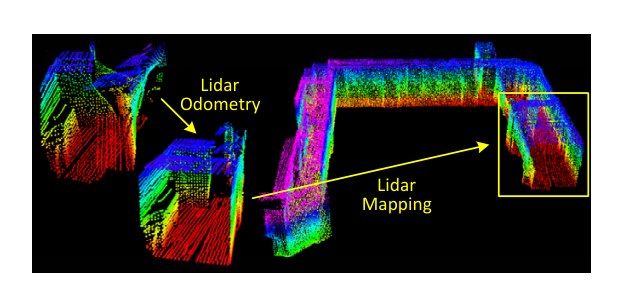
Fig. 1. The method aims at motion estimation and mapping using a moving 2-axis lidar. Since the laser points are received at different times, distortion is present in the point cloud due to motion of the lidar (shown in the left lidar cloud). Our proposed method decomposes the problem by two algorithms running in parallel. An odometry algorithm estimates velocity of the lidar and corrects distortion in the point cloud, then, a mapping algorithm matches and registers the point cloud to create a map. Combination of the two algorithms ensures feasibility of the problem to be solved in real-time.
图 1. 该方法旨在用一台运动中的两轴激光雷达做运动估计与建图。由于激光点在不同时刻到达,雷达运动会使点云出现扭曲(见左侧雷达点云)。我们提出的方法把问题分解为两条并行运行的算法。一条里程计算法估计雷达速度并纠正点云中的扭曲,随后一条建图算法匹配并配准点云以生成地图。二者结合,保证了这一问题可以实时求解。
I. INTRODUCTION
I. 引言
3D mapping remains a popular technology [1]–[3]. Mapping with lidars is common as lidars can provide high frequency range measurements where errors are relatively constant irrespective of the distances measured. In the case that the only motion of the lidar is to rotate a laser beam, registration of the point cloud is simple. However, if the lidar itself is moving as in many applications of interest, accurate mapping requires knowledge of the lidar pose during continuous laser ranging. One common way to solve the problem is using independent position estimation (e.g. by a GPS/INS) to register the laser points into a fixed coordinate system. Another set of methods use odometry measurements such as from wheel encoders or visual odometry systems [4], [5] to register the laser points. Since odometry integrates small incremental motions over time, it is bound to drift and much attention is devoted to reduction of the drift (e.g. using loop closure).
三维建图仍然是一项热门技术 [1]–[3]。用激光雷达建图很常见,因为雷达能提供高频测距,且误差相对稳定,并不随测距距离明显变化。若雷达的唯一运动只是旋转光束,点云配准很简单。然而,在许多我们关心的应用里,雷达自身也在运动,这时要准确建图,就必须知道连续测距过程中雷达的位姿。一种常见做法是用独立的位置估计(例如 GPS/INS)把激光点登记到固定坐标系中。另一类方法则用轮式编码器或视觉里程计等里程计测量 [4], [5] 来配准激光点。由于里程计是在时间上积分许多小的增量运动,必然会产生漂移,因此大量工作都花在减小漂移上(例如利用闭环)。
Here we consider the case of creating maps with low-drift odometry using a 2-axis lidar moving in 6-DOF. A key advantage of using a lidar is its insensitivity to ambient lighting and optical texture in the scene. Recent developments in lidars have reduced their size and weight. The lidars can be held by a person who traverses an environment [6], or even attached to a micro aerial vehicle [7]. Since our method is intended to push issues related to minimizing drift in odometry estimation, it currently does not involve loop closure.
这里我们考虑的情形是:用一台在六自由度中运动的两轴激光雷达,依靠低漂移里程计来建图。使用激光雷达的一个关键优点,是它对环境光照和场景中的光学纹理不敏感。近年来激光雷达的体积和重量都已减小,可以由人持着穿越环境 [6],甚至安装在微型飞行器上 [7]。由于我们的方法意在推进与减小里程计估计漂移相关的问题,目前并不包含闭环。
The method achieves both low-drift and low-computational complexity without the need for high accuracy ranging or inertial measurements. The key idea in obtaining this level of performance is the division of the typically complex problem of simultaneous localization and mapping (SLAM) [8], which seeks to optimize a large number of variables simultaneously, by two algorithms. One algorithm performs odometry at a high frequency but low fidelity to estimate velocity of the lidar. Another algorithm runs at a frequency of an order of magnitude lower for fine matching and registration of the point cloud. Although unnecessary, if an IMU is available, a motion prior can be provided to help account for high frequency motion. Specifically, both algorithms extract feature points located on sharp edges and planar surfaces, and match the feature points to edge line segments and planar surface patches, respectively. In the odometry algorithm, correspondences of the feature points are found by ensuring fast computation. In the mapping algorithm, the correspondences are determined by examining geometric distributions of local point clusters, through the associated eigenvalues and eigenvectors.
该方法在不必依赖高精度测距或惯性测量的情况下,同时获得了低漂移和低计算复杂度。达到这一性能的关键,是把通常很复杂的同时定位与建图(SLAM)问题 [8]——也就是要同时优化大量变量——拆成两条算法。一条算法以高频但较低保真度做里程计,用来估计雷达速度;另一条算法的频率低一个数量级,用于点云的精细匹配与配准。虽然并非必要,但如果有 IMU,也可以提供运动先验,以帮助应对高频运动。具体而言,两条算法都提取位于尖锐边沿和平面上的特征点,并分别把它们匹配到边线线段和平面小面片上。在里程计算法中,特征点的对应关系以保证计算快速的方式寻找;在建图算法中,对应关系则通过考察局部点簇的几何分布,以及与之相关的特征值和特征向量来确定。
By decomposing the original problem, an easier problem is solved first as online motion estimation. After which, mapping is conducted as batch optimization (similar to iterative closest point (ICP) methods [9]) to produce high-precision motion estimates and maps. The parallel algorithm structure ensures feasibility of the problem to be solved in real-time. Further, since the motion estimation is conducted at a higher frequency, the mapping is given plenty of time to enforce accuracy. When running at a lower frequency, the mapping algorithm is able to incorporate a large number of feature points and use sufficiently many iterations for convergence.
通过分解原问题,首先把一个更容易的问题作为在线运动估计来求解。随后,建图作为批优化来进行(类似于迭代最近点(ICP)方法 [9]),以产生高精度的运动估计和地图。并行的算法结构保证了这一问题可以实时求解。此外,由于运动估计在更高频率上进行,建图就有充足的时间来保证精度。当以较低频率运行时,建图算法能够纳入大量特征点,并使用足够多的迭代以达到收敛。
II. RELATED WORK
II. 相关工作
Lidar has become a useful range sensor in robot navigation [10]. For localization and mapping, most applications use 2D lidars [11]. When the lidar scan rate is high compared to its extrinsic motion, motion distortion within the scans can often be neglected. In this case, standard ICP methods [12] can be used to match laser returns between different scans. Additionally, a two-step method is proposed to remove the distortion [13]: an ICP based velocity estimation step is followed by a distortion compensation step, using the computed velocity. A similar technique is also used to compensate for the distortion introduced by a single-axis 3D lidar [14]. However, if the scanning motion is relatively slow, motion distortion can be severe. This is especially the case when a 2-axis lidar is used since one axis is typically much slower than the other. Often, other sensors are used to provide velocity measurements, with which, the distortion can be removed. For example, the lidar cloud can be registered by state estimation from visual odometry integrated with an IMU [15]. When multiple sensors such as a GPS/INS and wheel encoders are available concurrently, the problem is usually solved through an extended Kalman filer [16] or a particle filter [1]. These methods can create maps in real-time to assist path planning and collision avoidance in robot navigation.
激光雷达已成为机器人导航中有用的测距传感器 [10]。在定位与建图中,大多数应用使用二维激光雷达 [11]。当雷达扫描频率相对其外部运动足够高时,扫描内部的运动扭曲往往可以忽略。这时可以用标准 ICP 方法 [12] 在不同扫描之间匹配激光回波。此外,也有人提出两步法来去除扭曲 [13]:先用基于 ICP 的速度估计,再用算得的速度做扭曲补偿。类似技术也被用来补偿单轴三维激光雷达引入的扭曲 [14]。然而,若扫描运动相对较慢,运动扭曲会很严重。两轴激光雷达尤其如此,因为通常有一根轴比另一根慢得多。人们常常用其他传感器提供速度测量,并据此去除扭曲。例如,可以用与 IMU 结合的视觉里程计的状态估计来配准雷达点云 [15]。当 GPS/INS 和轮式编码器等多种传感器同时可用时,问题通常通过扩展卡尔曼滤波 [16] 或粒子滤波 [1] 来求解。这些方法可以实时建图,以辅助机器人导航中的路径规划与避障。
If a 2-axis lidar is used without aiding from other sensors, motion estimation and distortion correction become one problem. A method used by Barfoot et al. is to create visual images from laser intensity returns, and match visually distinct features [17] between images to recover motion of a ground vehicle [18]–[21]. The vehicle motion is modeled as constant velocity in [18], [19] and with Gaussian processes in [20], [21]. Our method uses a similar linear motion model as [18], [19] in the odometry algorithm, but with different types of features. The methods [18]–[21] involve visual features from intensity images and require dense point cloud. Our method extracts and matches geometric features in Cartesian space and has a lower requirement on the cloud density.
如果两轴激光雷达不借助其他传感器,运动估计与扭曲校正就变成同一个问题。Barfoot 等人使用的一种方法,是由激光强度回波生成视觉图像,再在图像间匹配视觉上显著的特征 [17],以恢复地面车辆的运动 [18]–[21]。车辆运动在 [18], [19] 中被建模为匀速,在 [20], [21] 中则用高斯过程建模。我们的方法在里程计算法中采用与 [18], [19] 类似的线性运动模型,但特征类型不同。[18]–[21] 使用来自强度图像的视觉特征,并需要稠密点云。我们的方法在笛卡尔空间中提取并匹配几何特征,对点云密度的要求更低。
The approach closest to ours is that of Bosse and Zlot [3], [6], [22]. They use a 2-axis lidar to obtain point cloud which is registered by matching geometric structures of local point clusters [22]. Further, they use multiple 2-axis lidars to map an underground mine [3]. This method incorporates an IMU and uses loop closure to create large maps. Proposed by the same authors, Zebedee is a mapping device composed of a 2D lidar and an IMU attached to a hand-bar through a spring [6]. Mapping is conducted by hand nodding the device. The trajectory is recovered by a batch optimization method that processes segmented datasets with boundary constraints added between the segments. In this method, the measurements of the IMU are used to register the laser points and the optimization is used to correct the IMU biases. In essence, Bosse and Zlot’s methods require batch processing to develop accurate maps and therefore are unsuitable for applications where maps are needed in real-time. In comparison, the proposed method in real-time produces maps that are qualitatively similar to those by Bosse and Zlot. The distinction is that our method can provide motion estimates for guidance of an autonomous vehicle. Further, the method takes advantage of the lidar scan pattern and point cloud distribution. Feature matching is realized ensuring computation speed and accuracy in the odometry and mapping algorithms, respectively.
与我们最接近的方法是 Bosse 与 Zlot 的工作 [3], [6], [22]。他们用两轴激光雷达获取点云,并通过匹配局部点簇的几何结构来配准 [22]。他们还用多台两轴激光雷达为地下矿井建图 [3]。该方法结合了 IMU,并利用闭环来生成大地图。同一作者提出的 Zebedee 是一种建图装置,由二维激光雷达和 IMU 经弹簧连接到手柄上构成 [6]。建图时用手点头式地摆动装置。轨迹由批优化方法恢复,该方法处理分段数据,并在各段之间加入边界约束。在这种方法中,IMU 测量用来配准激光点,优化则用来校正 IMU 偏差。本质上,Bosse 与 Zlot 的方法需要批处理才能做出准确地图,因此不适合需要实时地图的应用。相比之下,本文方法能够实时产生在外观上与 Bosse 和 Zlot 的结果定性相似的地图。区别在于,我们的方法还能提供用于自主车辆导引的运动估计。此外,该方法利用了激光雷达的扫描模式和点云分布。特征匹配分别在里程计算法中保证计算速度,在建图算法中保证精度。
III. NOTATIONS AND TASK DESCRIPTION
III. 符号与任务描述
The problem addressed in this paper is to perform ego-motion estimation with point cloud perceived by a 3D lidar, and build a map for the traversed environment. We assume that the lidar is pre-calibrated. We also assume that the angular and linear velocities of the lidar are smooth and continuous over time, without abrupt changes. The second assumption will be released by usage of an IMU, in Section VII-B.
本文要解决的问题是:利用三维激光雷达感知到的点云做自运动估计,并为所经过的环境建立地图。我们假定雷达已经预先标定。我们还假定雷达的角速度和线速度在时间上光滑连续,没有突变。第二个假定将在第 VII-B 节中通过使用 IMU 加以放松。
As a convention in this paper, we use right uppercase superscription to indicate the coordinate systems. We define a sweep as the lidar completes one time of scan coverage. We use right subscription , to indicate the sweeps, and to indicate the point cloud perceived during sweep . Let us define two coordinate systems as follows.
按本文的约定,我们用右上标表示坐标系。我们把雷达完成一次扫描覆盖称为一个扫描周期(sweep)。用右下标 , 表示各个扫描周期,并用 表示在扫描周期 中感知到的点云。两个坐标系定义如下。
• Lidar coordinate system is a 3D coordinate system with its origin at the geometric center of the lidar. The -axis is pointing to the left, the -axis is pointing upward, and the -axis is pointing forward. The coordinates of a point , , in are denoted as .
• 雷达坐标系 是一个三维坐标系,原点位于雷达的几何中心。 轴指向左, 轴指向上, 轴指向前。点 ,,在 中的坐标记为 。
• World coordinate system is a 3D coordinate system coinciding with at the initial position. The coordinates of a point , , in are .
• 世界坐标系 是一个三维坐标系,在初始位置与 重合。点 ,,在 中的坐标为 。
With assumptions and notations made, our lidar odometry and mapping problem can be defined as
在给出假定和符号之后,我们的激光雷达里程计与建图问题可以定义为
Problem: Given a sequence of lidar cloud , , compute the ego-motion of the lidar during each sweep , and build a map with for the traversed environment.
问题: 给定雷达点云序列 ,,计算雷达在每个扫描周期 中的自运动,并用 为所经过的环境建立地图。
IV. SYSTEM OVERVIEW
IV. 系统概述
A. Lidar Hardware
A. 激光雷达硬件
The study of this paper is validated on, but not limited to a custom built 3D lidar based on a Hokuyo UTM-30LX laser scanner. Through the paper, we will use data collected from the lidar to illustrate the method. The laser scanner has a field of view of with resolution and 40 lines/sec scan rate. The laser scanner is connected to a motor, which is controlled to rotate at an angular speed of between and with the horizontal orientation of the laser scanner as zero. With this particular unit, a sweep is a rotation from to or in the inverse direction (lasting for 1s). Here, note that for a continuous spinning lidar, a sweep is simply a semi-spherical rotation. An onboard encoder measures the motor rotation angle with a resolution of , with which, the laser points are projected into the lidar coordinates, .
本文的研究在一台基于 Hokuyo UTM-30LX 激光扫描器的自制三维激光雷达上验证,但不限于这一硬件。全文将用该雷达采集的数据来说明方法。该扫描器视场为 ,分辨率为 ,扫描速率为 40 线/秒。扫描器连接到一台电机,电机被控制以 的角速度在 与 之间旋转,并以扫描器的水平方位为零点。对这一特定装置,一个扫描周期是从 转到 ,或沿相反方向旋转(持续 1 秒)。这里需要说明的是,对连续旋转的激光雷达,一个扫描周期就是一次半球扫描。机载编码器以 的分辨率测量电机转角,并据此把激光点投影到雷达坐标系 中。
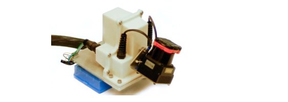
Fig. 2. The 3D lidar used in this study consists of a Hokuyo laser scanner driven by a motor for rotational motion, and an encoder that measures the rotation angle. The laser scanner has a field of view of with a resolution of . The scan rate is 40 lines/sec. The motor is controlled to rotate from to with the horizontal orientation of the laser scanner as zero.
图 2. 本研究使用的三维激光雷达由一台由电机带动旋转的 Hokuyo 激光扫描器和一台测量转角的编码器组成。扫描器视场为 ,分辨率为 。扫描速率为 40 线/秒。电机被控制从 转到 ,并以扫描器的水平方位为零点。
B. Software System Overview
B. 软件系统概述

Fig. 3. Block diagram of the lidar odometry and mapping software system.
图 3. 激光雷达里程计与建图软件系统的框图。
Fig. 3 shows a diagram of the software system. Let be the points received in a laser scan. During each sweep, is registered in . The combined point cloud during sweep forms . Then, is processed in two algorithms. The lidar odometry takes the point cloud and computes the motion of the lidar between two consecutive sweeps. The estimated motion is used to correct distortion in . The algorithm runs at a frequency around 10Hz. The outputs are further processed by lidar mapping, which matches and registers the undistorted cloud onto a map at a frequency of 1Hz. Finally, the pose transforms published by the two algorithms are integrated to generate a transform output around 10Hz, regarding the lidar pose with respect to the map. Section V and VI present the blocks in the software diagram in detail.
图 3 给出了软件系统的框图。设 为一次激光扫描中收到的点。在每个扫描周期内, 被登记到 中。扫描周期 内合并得到的点云记为 。随后, 由两条算法处理。激光雷达里程计接收该点云,并计算相邻两个扫描周期之间雷达的运动。估计得到的运动用来纠正 中的扭曲。该算法的运行频率约为 10Hz。其输出再交给激光雷达建图:建图算法以 1Hz 的频率,把去扭曲后的点云匹配并配准到地图上。最后,把两条算法发布的位姿变换加以组合,以约 10Hz 给出雷达相对地图的位姿。第 V 节和第 VI 节将详细介绍软件框图中的各个模块。
V. LIDAR ODOMETRY
V. 激光雷达里程计
A. Feature Point Extraction
A. 特征点提取
We start with extraction of feature points from the lidar cloud, . The lidar presented in Fig. 2 naturally generates unevenly distributed points in . The returns from the laser scanner has a resolution of within a scan. These points are located on a scan plane. However, as the laser scanner rotates at an angular speed of and generates scans at 40Hz, the resolution in the perpendicular direction to the scan planes is . Considering this fact, the feature points are extracted from using only information from individual scans, with co-planar geometric relationship.
我们首先从雷达点云 中提取特征点。图 2 所示的激光雷达会在 中自然产生分布不均匀的点。激光扫描器在一次扫描内的回波分辨率为 。这些点位于同一个扫描平面上。然而,扫描器以 的角速度旋转,并以 40Hz 产生扫描,因此垂直于扫描平面方向上的分辨率是 。考虑到这一点,特征点只利用各条扫描内部的信息,依据共面的几何关系,从 中提取。
We select feature points that are on sharp edges and planar surface patches. Let be a point in , , and let be the set of consecutive points of returned by the laser scanner in the same scan. Since the laser scanner generates point returns in CW or CCW order, contains half of its points on each side of and intervals between two points. Define a term to evaluate the smoothness of the local surface,
我们选择位于尖锐边沿和平面小面片上的特征点。设 为 中的一个点,,并设 为激光扫描器在同一条扫描中返回的、与 相邻的连续点集。由于扫描器按顺时针或逆时针顺序产生回波, 在 的两侧各包含一半的点,点与点之间间隔 。定义一个量来评价局部表面的光滑度,
The points in a scan are sorted based on the values, then feature points are selected with the maximum 's, namely, edge points, and the minimum 's, namely planar points. To evenly distribute the feature points within the environment, we separate a scan into four identical subregions. Each subregion can provide maximally 2 edge points and 4 planar points. A point can be selected as an edge or a planar point only if its value is larger or smaller than a threshold, and the number of selected points does not exceed the maximum.
一条扫描中的点按 值排序,然后选取 最大的点作为特征点,即边沿点,以及 最小的点,即平面点。为了使特征点在环境中分布均匀,我们把一条扫描分成四个相同的子区。每个子区最多提供 2 个边沿点和 4 个平面点。点 只有在其 值大于或小于某一阈值、且已选点数尚未超过上限时,才能被选为边沿点或平面点。
While selecting feature points, we want to avoid points whose surrounded points are selected, or points on local planar surfaces that are roughly parallel to the laser beams (point in Fig. 4(a)). These points are usually considered as unreliable. Also, we want to avoid points that are on boundary of occluded regions [23]. An example is shown in Fig. 4(b). Point is an edge point in the lidar cloud because its connected surface (the dotted line segment) is blocked by another object. However, if the lidar moves to another point of view, the occluded region can change and become observable. To avoid the aforementioned points to be selected, we find again the set of points . A point can be selected only if does not form a surface patch that is roughly parallel to the laser beam, and there is no point in that is disconnected from by a gap in the direction of the laser beam and is at the same time closer to the lidar then point (e.g. point in Fig. 4(b)).
在选取特征点时,我们希望避开周围点已被选中的点,以及位于与激光束近乎平行的局部平面上的点(图 4(a) 中的点 )。这类点通常被认为不可靠。我们还希望避开位于遮挡区域边界上的点 [23]。图 4(b) 给出了一个例子。点 在雷达点云中是一个边沿点,因为它所连接的表面(虚线段)被另一物体挡住。然而,如果雷达换到另一个视角,被遮挡的区域可能发生变化并变得可见。为避免选中上述这些点,我们再次找出点集 。点 只有在以下条件同时满足时才能被选中: 不会构成一块与激光束近乎平行的小面片,并且 中不存在这样的点——它与 在激光束方向上被间隙断开,同时又比点 更靠近雷达(例如图 4(b) 中的点 )。
In summary, the feature points are selected as edge points starting from the maximum value, and planar points starting from the minimum value, and if a point is selected,
综上所述,特征点按如下方式选取:边沿点从最大的 值开始取,平面点从最小的 值开始取;若某一点被选中,则须满足
• The number of selected edge points or planar points cannot exceed the maximum of the subregion, and
• 该子区中已选的边沿点或平面点数不能超过上限,并且
• None of its surrounding point is already selected, and
• 其周围点中没有已经被选中的点,并且
• It cannot be on a surface patch that is roughly parallel to the laser beam, or on boundary of an occluded region.
• 它不能位于与激光束近乎平行的小面片上,也不能位于遮挡区域的边界上。
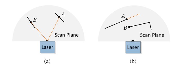
Fig. 4. (a) The solid line segments represent local surface patches. Point is on a surface patch that has an angle to the laser beam (the dotted orange line segments). Point is on a surface patch that is roughly parallel to the laser beam. We treat as a unreliable laser return and do not select it as a feature point. (b) The solid line segments are observable objects to the laser. Point is on the boundary of an occluded region (the dotted orange line segment), and can be detected as an edge point. However, if viewed from a different angle, the occluded region can change and become observable. We do not treat as a salient edge point or select it as a feature point.
图 4. (a) 实线段表示局部小面片。点 所在的小面片与激光束(橙色虚线段)成一定夹角。点 所在的小面片与激光束近乎平行。我们把 视为不可靠的激光回波,不把它选为特征点。(b) 实线段是激光能够观测到的物体。点 位于遮挡区域的边界上(橙色虚线段),因而可能被检测为边沿点。然而,若从另一个角度观察,被遮挡的区域可能发生变化并变得可见。我们不把 当作显著的边沿点,也不把它选为特征点。
An example of extracted feature points from a corridor scene is shown in Fig. 5. The edge points and planar points are labeled in yellow and red colors, respectively.
图 5 给出了从一个走廊场景中提取出的特征点示例。边沿点和平面点分别用黄色和红色标出。
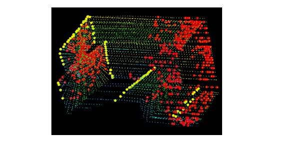
Fig. 5. An example of extracted edge points (yellow) and planar points (red) from lidar cloud taken in a corridor. Meanwhile, the lidar moves toward the wall on the left side of the figure at a speed of 0.5m/s, this results in motion distortion on the wall.
图 5. 从走廊中采集的雷达点云里提取出的边沿点(黄)和平面点(红)示例。与此同时,雷达以 0.5m/s 的速度朝图中左侧的墙面运动,因而墙面上出现了运动扭曲。
B. Finding Feature Point Correspondence
B. 寻找特征点对应
The odometry algorithm estimates motion of the lidar within a sweep. Let be the starting time of a sweep . At the end of each sweep, the point cloud perceived during the sweep, , is reprojected to time stamp , illustrated in Fig. 6. We denote the reprojected point cloud as . During the next sweep , is used together with the newly received point cloud, , to estimate the motion of the lidar.
里程计算法估计雷达在一个扫描周期内的运动。设 为扫描周期 的起始时刻。在每个扫描周期结束时,该周期内感知到的点云 被重新投影到时间戳 ,如图 6 所示。我们把重投影后的点云记为 。在下一个扫描周期 中, 与新收到的点云 一起用来估计雷达运动。

Fig. 6. Reprojecting point cloud to the end of a sweep. The blue colored line segment represents the point cloud perceived during sweep , . At the end of sweep , is reprojected to time stamp to obtain (the green colored line segment). Then, during sweep , and the newly perceived point cloud (the orange colored line segment) are used together to estimate the lidar motion.
图 6. 把点云重投影到一个扫描周期的结束时刻。蓝色线段表示扫描周期 中感知到的点云 。在扫描周期 结束时,把 重投影到时间戳 ,得到 (绿色线段)。随后,在扫描周期 中, 与新感知到的点云 (橙色线段)一起用来估计雷达运动。
Let us assume that both and are available for now, and start with finding correspondences between the two lidar clouds. With , we find edge points and planar points from the lidar cloud using the methodology discussed in the last section. Let and be the sets of edge points and planar points, respectively. We will find edge lines from as the correspondences for the points in , and planar patches as the correspondences for those in .
我们先假定 和 目前都已齐备,并从寻找两片雷达点云之间的对应关系开始。对 ,我们用上一节的方法从点云中找出边沿点和平面点。设 和 分别为边沿点集和平面点集。我们将在 中为 里的点寻找边线作为对应,为 里的点寻找平面小面片作为对应。
Note that at the beginning of sweep , is an empty set, which grows during the course of the sweep as more points are received. The lidar odometry recursively estimates the 6-DOF motion during the sweep, and gradually includes more points as increases. At each iteration, and are reprojected to the beginning of the sweep using the currently estimated transform. Let and be the reprojected point sets. For each point in and , we are going to find the closest neighbor point in . Here, is stored in a 3D KD-tree [24] for fast index.
需要注意的是,在扫描周期 开始时, 是空集,随着更多点的到达,它在该周期过程中逐渐增大。激光雷达里程计递归地估计该周期内的六自由度运动,并随着 的增大逐步纳入更多的点。在每次迭代中,用当前估计的变换把 和 重新投影到该扫描周期的起始时刻。设 和 为重投影后的点集。对 和 中的每个点,我们要在 中寻找最近邻点。这里把 存入三维 KD 树 [24],以便快速检索。
Fig. 7(a) represents the procedure of finding an edge line as the correspondence of an edge point. Let be a point in , . The edge line is represented by two points. Let be the closest neighbor of in , , and let be the closest neighbor of in the two consecutive scans to the scan of . forms the correspondence of . Then, to verify both and are edge points, we check the smoothness of the local surface based on (1). Here, we particularly require that and are from different scans considering that a single scan cannot contain more than one points from the same edge line. There is only one exception where the edge line is on the scan plane. If so, however, the edge line is degenerated and appears as a straight line on the scan plane, and feature points on the edge line should not be extracted in the first place.
图 7(a) 表示寻找边线作为某个边沿点之对应的过程。设 为 中的一个点,。边线由两点表示。设 为 在 中的最近邻,,再设 为 在与 所在扫描相邻的两条扫描中的最近邻。 构成 的对应。随后,为验证 和 都是边沿点,我们根据 (1) 式检查局部表面的光滑度。这里我们特别要求 和 来自不同扫描,因为同一条扫描不可能包含来自同一条边线的多于一个点。唯一的例外是边线就落在扫描平面上。若是这种情况,边线已经退化,在扫描平面上表现为一条直线,这条边线上的特征点本来就不应当被提取出来。
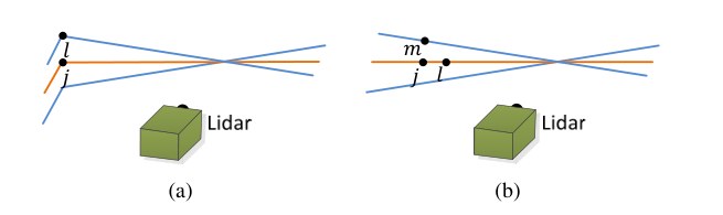
Fig. 7. Finding an edge line as the correspondence for an edge point in (a), and a planar patch as the correspondence for a planar point in (b). In both (a) and (b), is the closest point to the feature point, found in . The orange colored lines represent the same scan of , and the blue colored lines are the two consecutive scans. To find the edge line correspondence in (a), we find another point, , on the blue colored lines, and the correspondence is represented as . To find the planar patch correspondence in (b), we find another two points, and , on the orange and blue colored lines, respectively. The correspondence is .
图 7. 为 中的边沿点寻找边线作为对应 (a),以及为 中的平面点寻找平面小面片作为对应 (b)。在 (a) 和 (b) 中, 都是在 里找到的、距该特征点最近的点。橙色线表示 所在的同一条扫描,蓝色线是相邻的两条扫描。在 (a) 中寻找边线对应时,我们在蓝色线上再找一个点 ,对应表示为 。在 (b) 中寻找平面小面片对应时,我们再找两个点 和 ,分别位于橙色线和蓝色线上。对应为 。
Fig. 7(b) shows the procedure of finding a planar patch as the correspondence of a planar point. Let be a point in , . The planar patch is represented by three points. Similar to the last paragraph, we find the closest neighbor of in , denoted as . Then, we find another two points, and , as the closest neighbors of , one in the same scan of , and the other in the two consecutive scans to the scan of . This guarantees that the three points are non-collinear. To verify that , , and are all planar points, we check again the smoothness of the local surface based on (1).
图 7(b) 给出了寻找平面小面片作为某个平面点之对应的过程。设 为 中的一个点,。平面小面片由三个点表示。与上一段类似,我们在 中找出 的最近邻,记为 。然后另外找两个点 和 ,作为 的最近邻:一个在 所在的同一条扫描上,另一个在与 所在扫描相邻的两条扫描上。这样就保证了三点不共线。为验证 、 和 都是平面点,我们再次根据 (1) 式检查局部表面的光滑度。
With the correspondences of the feature points found, now we derive expressions to compute the distance from a feature point to its correspondence. We will recover the lidar motion by minimizing the overall distances of the feature points in the next section. We start with edge points. For a point , if is the corresponding edge line, , the point to line distance can be computed as
在找到特征点的对应关系之后,我们接下来推导特征点到其对应的距离表达式。下一节将通过最小化特征点的总体距离来恢复雷达运动。先看边沿点。对点 ,若 是对应的边线,,则点到直线的距离可写为
where , , and are the coordinates of points , , and in , respectively. Then, for a point , if is the corresponding planar patch, , the point to plane distance is
其中 、 和 分别是点 、 和 在 中的坐标。然后,对点 ,若 是对应的平面小面片,,则点到平面的距离为
where is the coordinates of point in \{L}.
其中 是点 在 中的坐标。
C. Motion Estimation
C. 运动估计
The lidar motion is modeled with constant angular and linear velocities during a sweep. This allows us to linear interpolate the pose transform within a sweep for the points that are received at different times. Let be the current time stamp, and recall that is the starting time of sweep . Let be the lidar pose transform between . contains rigid motion of the lidar in 6-DOF, , where , , and are translations along the -, -, and - axes of , respectively, and , , and are rotation angles, following the right-hand rule. Given a point , , let be its time stamp, and let be the pose transform between . can be computed by linear interpolation of ,
雷达运动被建模为在一个扫描周期内角速度和线速度保持恒定。这样就可以对在不同时刻到达的点,在扫描周期内对位姿变换做线性插值。设 为当前时间戳,并回顾 是扫描周期 的起始时刻。设 为区间 上的雷达位姿变换。 包含雷达的六自由度刚体运动,,其中 、 和 分别是沿 的 、 和 轴的平移,、 和 是按右手定则的转角。给定点 ,,设 为其时间戳,并设 为区间 上的位姿变换。 可由 线性插值得到,
Recall that and are the sets of edge points and planar points extracted from , and and are the sets of points reprojected to the beginning of the sweep, . To solved the lidar motion, we need to establish a geometric relationship between and , or and . Using the transform in (4), we can derive,
回顾 和 是从 中提取的边沿点集和平面点集, 和 则是被重投影到该扫描周期起始时刻 的点集。为了求解雷达运动,我们需要在 与 之间,或 与 之间建立几何关系。利用 (4) 式中的变换,可以推出
where is the coordinates of a point in or , is the corresponding point in or , is the -th to -th entries of , and is a rotation matrix defined by the Rodrigues formula [25],
其中 是 或 中点 的坐标, 是 或 中的对应点, 是 的第 至第 个分量, 则是由罗德里格斯公式 [25] 定义的旋转矩阵,
In the above equation, is the magnitude of the rotation,
在上式中, 是转角的大小,
is a unit vector representing the rotation direction,
是表示旋转方向的单位向量,
and is the skew symmetric matrix of [25].
而 是 的反对称矩阵 [25]。
Recall that (2) and (3) compute the distances between points in and and their correspondences. Combining (2) and (4)-(8), we can derive a geometric relationship between an edge point in and the corresponding edge line,
回顾 (2) 式和 (3) 式计算的是 和 中的点到其对应的距离。把 (2) 式与 (4)–(8) 式结合起来,可以推出 中一个边沿点与对应边线之间的几何关系,
Similarly, combining (3) and (4)-(8), we can establish another geometric relationship between a planar point in and the corresponding planar patch,
类似地,把 (3) 式与 (4)–(8) 式结合起来,可以建立 中一个平面点与对应平面小面片之间的几何关系,
Finally, we solve the lidar motion with the Levenberg-Marquardt method [26]. Stacking (9) and (10) for each feature point in and , we obtain a nonlinear function,
最后,我们用 Levenberg-Marquardt 方法 [26] 求解雷达运动。把 和 中每个特征点的 (9) 式和 (10) 式堆叠起来,得到一个非线性函数,
where each row of corresponds to a feature point, and contains the corresponding distances. We compute the Jacobian matrix of with respect to , denoted as , where . Then, (11) can be solved through nonlinear iterations by minimizing toward zero,
其中 的每一行对应一个特征点, 则包含相应的距离。我们计算 关于 的雅可比矩阵,记为 ,其中 。然后,通过非线性迭代把 向零最小化,即可求解 (11) 式,
is a factor determined by the Levenberg-Marquardt method.
是由 Levenberg-Marquardt 方法确定的因子。
Algorithm 1: Lidar Odometry
1 input : , , from the last recursion
2 output : , newly computed
3 begin
4 if at the beginning of a sweep then
5 ;
6 end
7 Detect edge points and planar points in , put the points in and , respectively;
8 for a number of iterations do
9 for each edge point in do
10 Find an edge line as the correspondence, then compute point to line distance based on (9) and stack the equation to (11);
11 end
12 for each planar point in do
13 Find a planar patch as the correspondence, then compute point to plane distance based on (10) and stack the equation to (11);
14 end
15 Compute a bisquare weight for each row of (11);
16 Update for a nonlinear iteration based on (12);
17 if the nonlinear optimization converges then
18 Break;
19 end
20 end
21 if at the end of a sweep then
22 Reproject each point in to and form ;
23 Return and ;
24 end
25 else
26 Return ;
27 end
28 end
算法 1: 激光雷达里程计
1 输入:上一轮递归得到的 ,,
2 输出:,新计算的
3 begin
4 if 处于一个扫描周期的起始时刻 then
5 ;
6 end
7 在 中检测边沿点和平面点,分别放入 和 ;
8 for 若干次迭代 do
9 for 中的每个边沿点 do
10 寻找一条边线作为对应,再根据 (9) 式计算点到直线的距离,并把该方程堆叠到 (11) 式;
11 end
12 for 中的每个平面点 do
13 寻找一块平面小面片作为对应,再根据 (10) 式计算点到平面的距离,并把该方程堆叠到 (11) 式;
14 end
15 为 (11) 式的每一行计算一个双平方权;
16 根据 (12) 式更新 ,完成一次非线性迭代;
17 if 非线性优化已经收敛 then
18 Break;
19 end
20 end
21 if 到达一个扫描周期的结束时刻 then
22 把 中的每个点重投影到 ,形成 ;
23 返回 和 ;
24 end
25 else
26 返回 ;
27 end
28 end
D. Lidar Odometry Algorithm
D. 激光雷达里程计算法
The lidar odometry algorithm is shown in Algorithm 1. The algorithm takes as inputs the point cloud from the last sweep, , the growing point cloud of the current sweep, , and the pose transform from the last recursion, . If a new sweep is started, is set to zero (line 4-6). Then, the algorithm extracts feature points from to construct and in line 7. For each feature point, we find its correspondence in (line 9-19). The motion estimation is adapted to a robust fitting [27]. In line 15, the algorithm assigns a bisquare weight for each feature point. The feature points that have larger distances to their correspondences are assigned with smaller weights, and the feature points with distances larger than a threshold are considered as outliers and assigned with zero weights. Then, in line 16, the pose transform is updated for one iteration. The nonlinear optimization terminates if convergence is found, or the maximum iteration number is met. If the algorithm reaches the end of a sweep, is reprojected to time stamp using the estimated motion during the sweep. Otherwise, only the transform is returned for the next round of recursion.
激光雷达里程计算法如算法 1 所示。算法的输入是上一扫描周期的点云 、当前扫描周期中正在增长的点云 ,以及上一轮递归得到的位姿变换 。若新的扫描周期刚开始,则把 置为零(第 4–6 行)。随后,算法在第 7 行从 中提取特征点,构造 和 。对每个特征点,我们在 中寻找其对应(第 9–19 行)。运动估计采用稳健拟合 [27]。在第 15 行,算法为每个特征点赋予一个双平方权:到其对应距离较大的特征点获得较小的权,距离超过阈值的特征点被视为离群点并赋零权。然后,在第 16 行对位姿变换做一次迭代更新。非线性优化在发现收敛、或达到最大迭代次数时终止。若算法到达一个扫描周期的结束时刻,则用该周期内估计得到的运动,把 重投影到时间戳 。否则,只返回变换 ,供下一轮递归使用。
VI. LIDAR MAPPING
VI. 激光雷达建图
The mapping algorithm runs at a lower frequency then the odometry algorithm, and is called only once per sweep. At the end of sweep , the lidar odometry generates a undistorted point cloud, , and simultaneously a pose transform, , containing the lidar motion during the sweep, between . The mapping algorithm matches and registers in the world coordinates, , illustrated in Fig. 8. To explain the procedure, let us define as the point cloud on the map, accumulated until sweep , and let be the pose of the lidar on the map at the end of sweep , . With the outputs from the lidar odometry, the mapping algorithm extents for one sweep from to , to obtain , and projects into the world coordinates, , denoted as . Next, the algorithm matches with by optimizing the lidar pose .
建图算法的运行频率比里程计算法低一个档次,每个扫描周期只调用一次。在扫描周期 结束时,激光雷达里程计生成一份去扭曲的点云 ,同时给出位姿变换 ,其中包含该周期内、区间 上的雷达运动。建图算法把 匹配并配准到世界坐标系 中,如图 8 所示。为说明这一过程,我们把截至扫描周期 累积在地图上的点云记为 ,并把扫描周期 结束时刻 雷达在地图上的位姿记为 。利用里程计的输出,建图算法把 从 延伸一个扫描周期到 ,得到 ,再把 投影到世界坐标系 中,记为 。随后,算法通过优化雷达位姿 ,把 与 匹配。
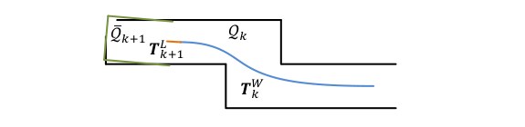
Fig. 8. Illustration of mapping process. The blue colored curve represents the lidar pose on the map, , generated by the mapping algorithm at sweep . The orange color curve indicates the lidar motion during sweep , , computed by the odometry algorithm. With and , the undistorted point cloud published by the odometry algorithm is projected onto the map, denoted as (the green colored line segments), and matched with the existing cloud on the map, (the black colored line segments).
图 8. 建图过程示意。蓝色曲线表示建图算法在扫描周期 生成的、雷达在地图上的位姿 。橙色曲线表示里程计算法算出的、扫描周期 内的雷达运动 。利用 和 ,把里程计算法发布的去扭曲点云投影到地图上,记为 (绿色线段),并与地图上已有的点云 (黑色线段)相匹配。
The feature points are extracted in the same way as in Section V-A, but 10 times of feature points are used. To find correspondences for the feature points, we store the point cloud on the map, , in 10m cubic areas. The points in the cubes that intersect with are extracted and stored in a 3D KD-tree [24]. We find the points in within a certain region around the feature points. Let be a set of surrounding points. For an edge point, we only keep points on edge lines in , and for a planar point, we only keep points on planar patches. Then, we compute the covariance matrix of , denoted as , and the eigenvalues and eigenvectors of , denoted as and , respectively. If is distributed on an edge line, contains one eigenvalue significantly larger than the other two, and the eigenvector in associated with the largest eigenvalue represents the orientation of the edge line. On the other hand, if is distributed on a planar patch, contains two large eigenvalues with the third one significantly smaller, and the eigenvector in associated with the smallest eigenvalue denotes the orientation of the planar patch. The position of the edge line or the planar patch is determined by passing through the geometric center of .
特征点的提取方式与第 V-A 节相同,但使用的特征点数量约为原来的 10 倍。为了给这些特征点寻找对应,我们把地图上的点云 按 10m 边长的立方区域存放。与 相交的立方体中的点被取出,并存入一棵三维 KD 树 [24]。我们在 中寻找特征点周围一定区域内的点。设 为周围点的集合。对边沿点,我们只在 中保留位于边线上的点;对平面点,则只保留位于平面小面片上的点。随后,计算 的协方差矩阵,记为 ,以及 的特征值和特征向量,分别记为 和 。若 分布在一条边线上, 中有一个特征值明显大于另外两个,与最大特征值相对应的、 中的特征向量表示这条边线的方向。另一方面,若 分布在一块平面小面片上, 中有两个较大的特征值,第三个则明显更小,与最小特征值相对应的特征向量给出该小面片的法向。边线或小面片的位置由通过 几何中心来确定。
To compute the distance from a feature point to its correspondence, we select two points on an edge line, and three points on a planar patch. This allows the distances to be computed using the same formulations as (2) and (3). Then, an equation is derived for each feature point as (9) or (10), but different in that all points in share the same time stamp, . The nonlinear optimization is solved again by a robust fitting [27] through the Levenberg-Marquardt method [26], and is registered on the map. To evenly distribute the points, the map cloud is downsized by a voxel grid filter [28] with the voxel size of 5cm cubes.
为计算特征点到其对应的距离,我们在边线上取两个点,在平面小面片上取三个点。这样就可以用与 (2) 式和 (3) 式相同的公式来计算距离。随后,为每个特征点写出形如 (9) 式或 (10) 式的方程,不同之处在于 中的所有点共享同一个时间戳 。非线性优化同样采用稳健拟合 [27],通过 Levenberg-Marquardt 方法 [26] 求解,并把 配准到地图上。为使点的分布更均匀,用边长为 5cm 的体素栅格滤波器 [28] 对地图点云降采样。

Fig. 9. Integration of pose transforms. The blue colored region illustrates the lidar pose from the mapping algorithm, , generated once per sweep. The orange colored region is the lidar motion within the current sweep, , computed by the odometry algorithm. The motion estimation of the lidar is the combination of the two transforms, at the same frequency as .
图 9. 位姿变换的组合。蓝色区域表示建图算法给出的雷达位姿 ,每个扫描周期生成一次。橙色区域是里程计算法算出的、当前扫描周期内的雷达运动 。雷达的运动估计由这两个变换组合而成,输出频率与 相同。
Integration of the pose transforms is illustrated in Fig. 9. The blue colored region represents the pose output from the lidar mapping, , generated once per sweep. The orange colored region represents the transform output from the lidar odometry, , at a frequency round 10Hz. The lidar pose with respect to the map is the combination of the two transforms, at the same frequency as the lidar odometry.
位姿变换的组合如图 9 所示。蓝色区域表示激光雷达建图给出的位姿输出 ,每个扫描周期生成一次。橙色区域表示激光雷达里程计给出的变换输出 ,频率约为 10Hz。雷达相对地图的位姿是这两个变换的组合,输出频率与里程计相同。
VII. EXPERIMENTS
VII. 实验
During experiments, the algorithms processing the lidar data run on a laptop computer with 2.5GHz quad cores and 6Gib memory, on robot operating system (ROS) [29] in Linux. The method consumes a total of two cores, the odometry and mapping programs run on two separate cores. Our software code and datasets are publicly available.
实验中,处理雷达数据的算法运行在一台 2.5GHz 四核、6Gib 内存的笔记本电脑上,操作系统为 Linux 上的机器人操作系统(ROS)[29]。该方法一共占用两个核,里程计程序和建图程序分别在两个核上运行。我们的软件代码和数据集已公开。
1 wiki.ros.org/loam_back_and_forth
2 wiki.ros.org/loam_continuous
A. Indoor & Outdoor Tests
A. 室内与室外试验
The method has been tested in indoor and outdoor environments. During indoor tests, the lidar is placed on a cart together with a battery and a laptop computer. One person pushes the cart and walks. Fig. 10(a) and Fig. 10(c) show maps built in two representative indoor environments, a narrow and long corridor and a large lobby. Fig. 10(b) and Fig. 10(d) show two photos taken from the same scenes. In outdoor tests, the lidar is mounted to the front of a ground vehicle. Fig. 10(e) and Fig. 10(g) show maps generated from a vegetated road and an orchard between two rows of trees, and photos are presented in Fig. 10(f) and Fig. 10(h), respectively. During all tests, the lidar moves at a speed of 0.5m/s.
该方法已在室内和室外环境中测试。室内试验时,雷达与电池、笔记本电脑一起放在手推车上,由一人推着车行走。图 10(a) 和图 10(c) 给出了两个有代表性的室内环境中建成的地图:一条又窄又长的走廊,以及一个较大的大厅。图 10(b) 和图 10(d) 是同一场景拍下的照片。室外试验时,雷达安装在地面车辆的前方。图 10(e) 和图 10(g) 给出了植被道路以及两排树之间的果园中生成的地图,对应照片分别见图 10(f) 和图 10(h)。所有试验中,雷达的运动速度都是 0.5m/s。
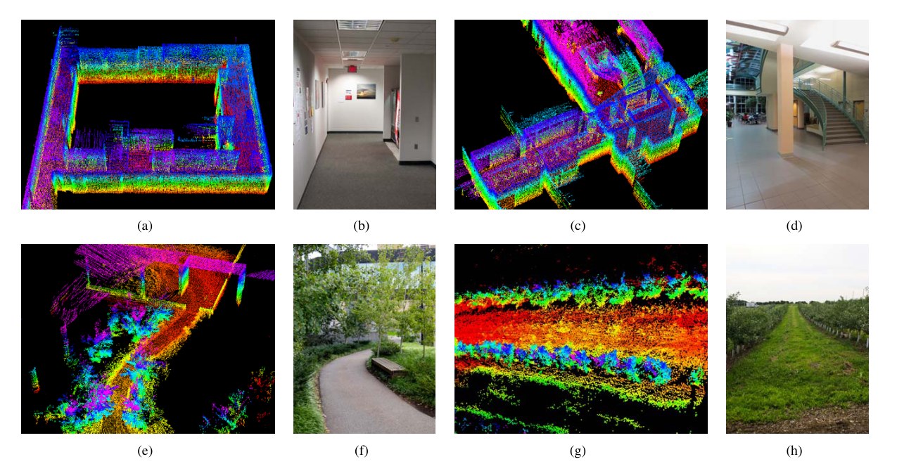
Fig. 10. Maps generated in (a)-(b) a narrow and long corridor, (c)-(d) a large lobby, (e)-(f) a vegetated road, and (g)-(h) an orchard between two rows of trees. The lidar is placed on a cart in indoor tests, and mounted on a ground vehicle in outdoor tests. All tests use a speed of 0.5m/s.
图 10. 在 (a)-(b) 一条又窄又长的走廊、(c)-(d) 一个较大的大厅、(e)-(f) 一条植被道路,以及 (g)-(h) 两排树之间的果园中生成的地图。室内试验时雷达放在手推车上,室外试验时安装在地面车辆上。所有试验的速度都是 0.5m/s。
To evaluate local accuracy of the maps, we collect a second set of lidar clouds from the same environments. The lidar is kept stationary and placed at a few different places in each environment during data selection. The two point clouds are matched and compared using the point to plane ICP method [9]. After matching is complete, the distances between one point cloud and the corresponding planer patches in the second point cloud are considered as matching errors. Fig. 11 shows the density of error distributions. It indicates smaller matching errors in indoor environments than in outdoor. The result is reasonable because feature matching in natural environments is less exact than in manufactured environments.
为评估地图的局部精度,我们在同样的环境中另外采集了一组雷达点云。采集时雷达保持静止,并在每个环境中放置于若干不同位置。两片点云用点到平面的 ICP 方法 [9] 进行匹配和比较。匹配完成后,一片点云到第二片点云中相应平面小面片的距离被当作匹配误差。图 11 给出了误差分布的密度。结果表明,室内环境中的匹配误差小于室外。这一结果是合理的,因为自然场景里的特征匹配没有人造环境那么确切。
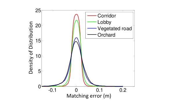
Fig. 11. Matching errors for corridor (red), lobby (green), vegetated road (blue) and orchard (black), corresponding to the four scenes in Fig. 10.
图 11. 走廊(红)、大厅(绿)、植被道路(蓝)和果园(黑)的匹配误差,分别对应图 10 中的四个场景。
Additionally, we conduct tests to measure accumulated drift of the motion estimate. We choose corridor for indoor experiments that contains a closed loop. This allows us to start and finish at the same place. The motion estimation generates a gap between the starting and finishing positions, which indicates the amount of drift. For outdoor experiments, we choose orchard environment. The ground vehicle that carries the lidar is equipped with a high accuracy GPS/INS for ground truth acquisition. The measured drifts are compared to the distance traveled as the relative accuracy, and listed in Table I. Specifically, Test 1 uses the same datasets with Fig. 10(a) and Fig. 10(g). In general, the indoor tests have a relative accuracy around 1% and the outdoor tests are around 2.5%.
此外,我们还做了试验来测量运动估计的累积漂移。室内试验选择含有闭合回路的走廊,这样就可以在同一地点出发并返回。运动估计会在起点和终点之间留下一段空隙,这段空隙就反映了漂移的大小。室外试验选择果园环境。搭载雷达的地面车辆配有高精度 GPS/INS,用来获取真值。测得的漂移与行驶距离相比,作为相对精度列于表 I。具体而言,试验 1 使用的是与图 10(a) 和图 10(g) 相同的数据集。总体来看,室内试验的相对精度约为 1%,室外试验约为 2.5%。
| Environment | Test 1 | Test 2 | ||
|---|---|---|---|---|
| Distance | Error | Distance | Error | |
| Corridor | 58m | 0.9% | 46m | 1.1% |
| Orchard | 52m | 2.3% | 67m | 2.8% |
TABLE I
RELATIVE ERRORS FOR MOTION ESTIMATION DRIFT.
| 环境 | 试验 1 | 试验 2 | ||
|---|---|---|---|---|
| 距离 | 误差 | 距离 | 误差 | |
| 走廊 | 58m | 0.9% | 46m | 1.1% |
| 果园 | 52m | 2.3% | 67m | 2.8% |
表 I
运动估计漂移的相对误差。
B. Assistance from an IMU
B. 来自 IMU 的辅助
We attach an Xsens MTi-10 IMU to the lidar to deal with fast velocity changes. The point cloud is preprocessed in two ways before sending to the proposed method, 1) with orientation from the IMU, the point cloud received in one sweep is rotated to align with the initial orientation of the lidar in that sweep, 2) with acceleration measurement, the motion distortion is partially removed as if the lidar moves at a const velocity during the sweep. The point cloud is then processed by the lidar odometry and mapping programs.
我们在雷达上安装一台 Xsens MTi-10 IMU,以应对速度的快速变化。点云在送入本文方法之前先做两方面预处理:1)利用 IMU 给出的姿态,把一个扫描周期内收到的点云旋转到与该周期开始时雷达的初始姿态对齐;2)利用加速度测量,部分去除运动扭曲,使点云看起来如同雷达在该周期内以恒定速度运动。随后,点云再由激光雷达里程计和建图程序处理。
The IMU orientation is obtained by integrating angular rates from a gyro and readings from an accelerometer in a Kalman filter [1]. Fig. 12(a) shows a sample result. A person holds the lidar and walks on a staircase. When computing the red curve, we use orientation provided by the IMU, and our method only estimates translation. The orientation drifts over during 5 mins of data collection. The green curve relies only on the optimization in our method, assuming no IMU is available. The blue curve uses the IMU data for preprocessing followed by the proposed method. We observe small difference between the green and blue curves. Fig. 12(b) presents the map corresponding to the blue curve. In Fig. 12(c), we compare two closed views of the maps in the yellow rectangular in Fig. 12(b). The upper and lower figures correspond to the blue and green curves, respectively. Careful comparison finds that the edges in the upper figure are sharper.
IMU 的姿态由陀螺仪角速度与加速度计读数在卡尔曼滤波器 [1] 中积分得到。图 12(a) 给出了一个示例结果。一人手持雷达在楼梯上行走。计算红色曲线时,我们使用 IMU 提供的姿态,本文方法只估计平移。在 5 分钟的数据采集中,姿态漂移超过了 。绿色曲线只依赖本文方法中的优化,假定没有 IMU 可用。蓝色曲线先用 IMU 数据做预处理,再使用本文方法。我们观察到绿色曲线与蓝色曲线差别不大。图 12(b) 给出了与蓝色曲线相对应的地图。在图 12(c) 中,我们比较了图 12(b) 黄色矩形框内地图的两处局部放大。上图和下图分别对应蓝色曲线和绿色曲线。仔细比较可以发现,上图中的边沿更为锐利。
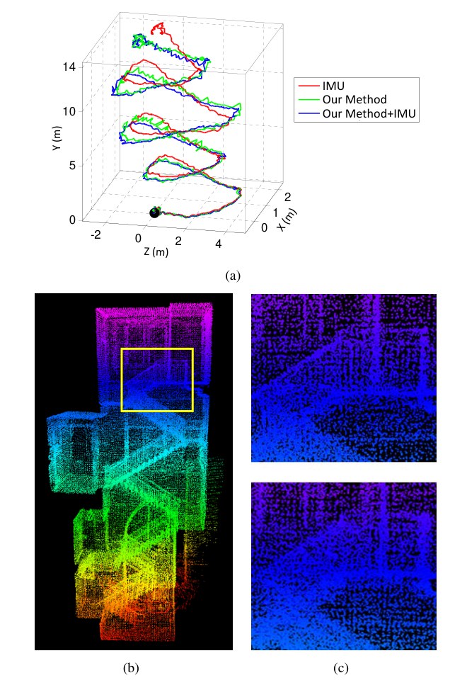
Fig. 12. Comparison of results with/without aiding from an IMU. A person holds the lidar and walks on a staircase. The black dot is the starting point. In (a), the red curve is computed using orientation from the IMU and translation estimated by our method, the green curve relies on the optimization in our method only, and the blue curve uses the IMU data for preprocessing followed by the method. (b) is the map corresponding to the blue curve. In (c), the upper and lower figures correspond to the blue and green curves, respectively, using the region labeled by the yellow rectangular in (b). The edges in the upper figure are sharper, indicating more accuracy on the map.
图 12. 有无 IMU 辅助时的结果比较。一人手持雷达在楼梯上行走。黑点为起点。在 (a) 中,红色曲线用 IMU 的姿态和本文方法估计的平移算出,绿色曲线只依赖本文方法中的优化,蓝色曲线则先用 IMU 数据做预处理再使用本文方法。(b) 是与蓝色曲线相对应的地图。在 (c) 中,上图和下图分别对应蓝色曲线和绿色曲线,截取的是 (b) 中黄色矩形框标出的区域。上图中的边沿更为锐利,说明地图更为准确。
Table II compares relative errors in motion estimation with and without using the IMU. The lidar is held by a person walking at a speed of 0.5m/s and moving the lidar up and down at a magnitude around 0.5m. The ground truth is manually measured by a tape ruler. In all four tests, using the proposed method with assistance from the IMU gives the highest accuracy, while using orientation from the IMU only leads to the lowest accuracy. The results indicate that the IMU is effective in canceling the nonlinear motion, with which, the proposed method handles the linear motion.
表 II 比较了使用和不使用 IMU 时运动估计的相对误差。雷达由人以 0.5m/s 的速度手持行走,同时把雷达上下摆动约 0.5m。真值用手持卷尺测量。在全部四组试验中,用本文方法并借助 IMU 得到的精度最高,而只用 IMU 姿态得到的精度最低。结果表明,IMU 能有效抵消非线性运动,在此基础上,本文方法再处理线性运动。
| Environment | Distance | Error | ||
|---|---|---|---|---|
| IMU | Ours | Ours+IMU | ||
| Corridor | 32m | 16.7% | 2.1% | 0.9% |
| Lobby | 27m | 11.7% | 1.7% | 1.3% |
| Vegetated road | 43m | 13.7% | 4.4% | 2.6% |
| Orchard | 51m | 11.4% | 3.7% | 2.1% |
TABLE II
MOTION ESTIMATION ERRORS WITH/WITHOUT USING IMU.
| 环境 | 距离 | 误差 | ||
|---|---|---|---|---|
| IMU | 本文方法 | 本文方法+IMU | ||
| 走廊 | 32m | 16.7% | 2.1% | 0.9% |
| 大厅 | 27m | 11.7% | 1.7% | 1.3% |
| 植被道路 | 43m | 13.7% | 4.4% | 2.6% |
| 果园 | 51m | 11.4% | 3.7% | 2.1% |
表 II
使用或不使用 IMU 时的运动估计误差。
C. Tests with KITTI Datasets
C. 在 KITTI 数据集上的试验
We have also evaluated our method using datasets from the KITTI odometry benchmark [30], [31]. The datasets are carefully registered with sensors mounted on top of a passenger vehicle (Fig. 13(a)) driving on structured roads. The vehicle is equipped with a Velodyne lidar, color/monochrome stereo cameras, and a high accuracy GPS/INS for ground truth purposes. The lidar data is logged at 10Hz and used by our method for odometry estimation. Due to space issue, we are not able to include the results. However, we encourage readers to review our results on the benchmark website.
我们还用 KITTI 里程计基准 [30], [31] 中的数据集评测了该方法。这些数据由安装在乘用车顶部的传感器仔细配准而得(图 13(a)),车辆行驶在结构化道路上。车上配有一台 的 Velodyne 激光雷达、彩色/单色立体相机,以及用于获取真值的高精度 GPS/INS。雷达数据以 10Hz 记录,并由我们的方法用来估计里程计。限于篇幅,我们无法在文中给出结果。不过,我们鼓励读者到基准网站上查看我们的结果。
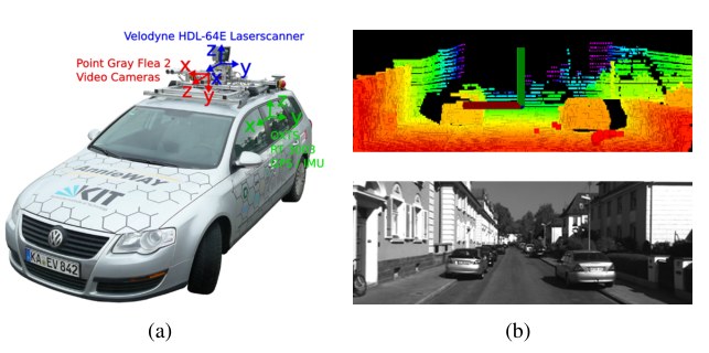
Fig. 13. (a) Sensor configuration and vehicle used by the KITTI benchmark. The vehicle is mounted with a Velodyne lidar, stereo cameras, and a high accuracy GPS/INS for ground truth acquisition. Our method uses data from the Velodyne lidar only. (b) A sample lidar cloud (upper figure) and the corresponding visual image (lower figure) from an urban scene.
图 13. (a) KITTI 基准所使用的传感器配置与车辆。车上安装了 Velodyne 激光雷达、立体相机,以及用于获取真值的高精度 GPS/INS。我们的方法只使用 Velodyne 激光雷达的数据。(b) 一个城市场景中的雷达点云样例(上图)及对应的视觉图像(下图)。
The datasets mainly cover three types of environments: “urban” with buildings around, “country” on small roads with vegetations in the scene, and “highway” where roads are wide and the surrounding environment is relatively clean. Fig. 13(b) shows a sample lidar cloud and the corresponding visual image from an urban environment. The overall driving distance included in the datasets is 39.2km. Upon uploading of the vehicle trajectories, the accuracy and ranking are automatically calculated by the benchmark server. Our method is ranked #1 among all methods evaluated by the benchmark irrespective of sensing modality, including state of the art stereo visual odometry [32], [33]. The average position error is 0.88% of the distance traveled, generated using trajectory segments at 100m, 200m, ..., 800m lengthes in 3D coordinates.
这些数据集主要覆盖三类环境:“urban”(城市),周围有建筑物;“country”(乡村),行驶在小路上、场景中有植被;以及“highway”(公路),道路较宽、周围环境相对空旷。图 13(b) 给出了一个城市环境中的雷达点云样例及对应的视觉图像。数据集中包含的总行驶距离为 39.2km。车辆轨迹上传后,精度和排名由基准服务器自动计算。我们的方法在该基准评测过的所有方法中排名第一,不论使用何种传感方式,其中包括当时最先进的立体视觉里程计 [32], [33]。平均位置误差为行驶距离的 0.88%,这一数字由长度为 100m、200m、……、800m 的三维轨迹段计算得到。
VIII. CONCLUSION AND FUTURE WORK
VIII. 结论与后续工作
Motion estimation and mapping using point cloud from a rotating laser scanner can be difficult because the problem involves recovery of motion and correction of motion distortion in the lidar cloud. The proposed method divides and solves the problem by two algorithms running in parallel: the lidar odometry conduces coarse processing to estimate velocity at a higher frequency, while the lidar mapping performs fine processing to create maps at a lower frequency. Cooperation of the two algorithms allows accurate motion estimation and mapping in real-time. Further, the method can take advantage of the lidar scan pattern and point cloud distribution. Feature matching is made to ensure fast computation in the odometry algorithm, and to enforce accuracy in the mapping algorithm. The method has been tested both indoor and outdoor as well as on the KITTI odometry benchmark.
用旋转激光扫描器得到的点云做运动估计与建图并不容易,因为问题同时涉及恢复运动,以及纠正雷达点云中的运动扭曲。本文方法把问题拆开,由两条并行运行的算法来求解:激光雷达里程计以较高频率做粗处理以估计速度,激光雷达建图则以较低频率做精细处理以生成地图。两条算法相互配合,使准确的运动估计与建图可以实时完成。此外,该方法还能利用激光雷达的扫描模式和点云分布。特征匹配在里程计算法中保证计算快速,在建图算法中保证精度。该方法已在室内、室外以及 KITTI 里程计基准上得到测试。
Since the current method does not recognize loop closure, our future work involves developing a method to fix motion estimation drift by closing the loop. Also, we will integrate the output of our method with an IMU in a Kalman filter to further reduce the motion estimation drift.
由于当时方法还不会识别闭环,后续工作包括发展一种通过闭环来修正运动估计漂移的方法。我们还将把方法的输出与 IMU 一起放入卡尔曼滤波器,以进一步减小运动估计漂移。
REFERENCES
参考文献
[1] S. Thrun, W. Burgard, and D. Fox, Probabilistic Robotics. Cambridge, MA, The MIT Press, 2005.
[2] M. Kaess, H. Johannsson, R. Roberts, V. Ila, J. Leonard, and F. Dellaert, “iSAM2: Incremental smoothing and mapping using the bayes tree,” The International Journal of Robotics Research, vol. 31, pp. 217–236, 2012.
[3] R. Zlot and M. Bosse, “Efficient large-scale 3D mobile mapping and surface reconstruction of an underground mine,” in The 7th International Conference on Field and Service Robots, Matsushima, Japan, July 2012.
[4] K. Konolige, M. Agrawal, and J. Sol, “Large-scale visual odometry for rough terrain,” Robotics Research, vol. 66, p. 201212, 2011.
[5] D. Nister, O. Naroditsky, and J. Bergen, “Visual odometry for ground vechicle applications,” Journal of Field Robotics, vol. 23, no. 1, pp. 3–20, 2006.
[6] M. Bosse, R. Zlot, and P. Flick, “Zebedee: Design of a spring-mounted 3-D range sensor with application to mobile mapping,” vol. 28, no. 5, pp. 1104–1119, 2012.
[7] S. Shen and N. Michael, “State estimation for indoor and outdoor operation with a micro-aerial vehicle,” in International Symposium on Experimental Robotics (ISER), Quebec City, Canada, June 2012.
[8] H. Durrant-Whyte and T. Bailey, “Simultaneous localization and mapping: part i the essential algorithms,” IEEE Robotics & Automation Magazine, vol. 13, no. 2, pp. 99–110, 2006.
[9] S. Rusinkiewicz and M. Levoy, “Efficient variants of the ICP algorithm,” in Third International Conference on 3D Digital Imaging and Modeling (3DIM), Quebec City, Canada, June 2001.
[10] A. Nuchter, K. Lingemann, J. Hertzberg, and H. Surmann, “6D SLAM–3D mapping outdoor environments,” Journal of Field Robotics, vol. 24, no. 8-9, pp. 699–722, 2007.
[11] S. Kohlbrecher, O. von Stryk, J. Meyer, and U. Klingauf, “A flexible and scalable SLAM system with full 3D motion estimation,” in IEEE International Symposium on Safety, Security, and Rescue Robotics, Kyoto, Japan, September 2011.
[12] F. Pomerleau, F. Colas, R. Siegwart, and S. Magnenat, “Comparing ICP variants on real-world data sets,” Autonomous Robots, vol. 34, no. 3, pp. 133–148, 2013.
[13] S. Hong, H. Ko, and J. Kim, “VICP: Velocity updating iterative closest point algorithm,” in IEEE International Conference on Robotics and Automation (ICRA), Anchorage, Alaska, May 2010.
[14] F. Moosmann and C. Stiller, “Velodyne SLAM,” in IEEE Intelligent Vehicles Symposium (IV), Baden-Baden, Germany, June 2011.
[15] S. Scherer, J. Rehder, S. Achar, H. Cover, A. Chambers, S. Nuske, and S. Singh, “River mapping from a flying robot: state estimation, river detection, and obstacle mapping,” Autonomous Robots, vol. 32, no. 5, pp. 1 – 26, May 2012.
[16] M. Montemerlo, S. Thrun, D. Koller, and B. Wegbreit, “FastSLAM: A factored solution to the simultaneous localization and mapping problem,” in The AAAI Conference on Artificial Intelligence, Edmonton, Canada, July 2002.
[17] H. Bay, A. Ess, T. Tuytelaars, and L. Gool, “SURF: Speeded up robust features,” Computer Vision and Image Understanding, vol. 110, no. 3, pp. 346–359, 2008.
[18] H. Dong and T. Barfoot, “Lighting-invariant visual odometry using lidar intensity imagery and pose interpolation,” in The 7th International Conference on Field and Service Robots, Matsushima, Japan, July 2012.
[19] S. Anderson and T. Barfoot, “RANSAC for motion-distorted 3D visual sensors,” in 2013 IEEE/RSJ International Conference on Intelligent Robots and Systems (IROS), Tokyo, Japan, Nov. 2013.
[20] C. H. Tong and T. Barfoot, “Gaussian process gauss-newton for 3D laser-based visual odometry,” in IEEE International Conference on Robotics and Automation (ICRA), Karlsruhe, Germany, May 2013.
[21] S. Anderson and T. Barfoot, “Towards relative continuous-time SLAM,” in IEEE International Conference on Robotics and Automation (ICRA), Karlsruhe, Germany, May 2013.
[22] M. Bosse and R. Zlot, “Continuous 3D scan-matching with a spinning 2D laser,” in IEEE International Conference on Robotics and Automation, Kobe, Japan, May 2009.
[23] Y. Li and E. Olson, “Structure tensors for general purpose LIDAR feature extraction,” in IEEE International Conference on Robotics and Automation, Shanghai, China, May 9-13 2011.
[24] M. de Berg, M. van Kreveld, M. Overmars, and O. Schwarzkopf, Computation Geometry: Algorithms and Applications, 3rd Edition. Springer, 2008.
[25] R. Murray and S. Sastry, A mathematical introduction to robotic manipulation. CRC Press, 1994.
[26] R. Hartley and A. Zisserman, Multiple View Geometry in Computer Vision. New York, Cambridge University Press, 2004.
[27] R. Andersen, “Modern methods for robust regression.” Sage University Paper Series on Quantitative Applications in the Social Sciences, 2008.
[28] R. B. Rusu and S. Cousins, “3D is here: Point Cloud Library (PCL),” in IEEE International Conference on Robotics and Automation (ICRA), Shanghai, China, May 9-13 2011.
[29] M. Quigley, B. Gerkey, K. Conley, J. Faust, T. Foote, J. Leibs, E. Berger, R. Wheeler, and A. Ng, “ROS: An open-source robot operating system,” in Workshop on Open Source Software (Collocated with ICRA 2009), Kobe, Japan, May 2009.
[30] A. Geiger, P. Lenz, and R. Urtasun, “Are we ready for autonomous driving? The kitti vision benchmark suite,” in IEEE Conference on Computer Vision and Pattern Recognition (CVPR), 2012, pp. 3354–3361.
[31] A. Geiger, P. Lenz, C. Stiller, and R. Urtasun, “Vision meets robotics: The KITTI dataset,” International Journal of Robotics Research, no. 32, pp. 1229–1235, 2013.
[32] H. Badino and T. Kanade, “A head-wearable short-baseline stereo system for the simultaneous estimation of structure and motion,” in IAPR Conference on Machine Vision Application, Nara, Japan, 2011.
[33] A. Y. H. Badino and T. Kanade, “Visual odometry by multi-frame feature integration,” in Workshop on Computer Vision for Autonomous Driving (Collocated with ICCV 2013), Sydney, Australia, 2013.