Lift, Splat, Shoot: Encoding Images from Arbitrary Camera Rigs by Implicitly Unprojecting to 3D

Lift, Splat, Shoot：通过隐式反投影到三维，对任意相机配置的图像编码

Jonah Philion    Sanja Fidler Affiliation:  NVIDIA    University of Toronto    Vector Institute

Abstract

摘要

The goal of perception for autonomous vehicles is to extract semantic representations from multiple sensors and fuse these representations into a single “bird’s-eye-view” coordinate frame for consumption by motion planning. We propose a new end-to-end architecture that directly extracts a bird’s-eye-view representation of a scene given image data from an arbitrary number of cameras. The core idea behind our approach is to “lift” each image individually into a frustum of features for each camera, then “splat” all frustums into a rasterized bird’s-eye-view grid. By training on the entire camera rig, we provide evidence that our model is able to learn not only how to represent images but how to fuse predictions from all cameras into a single cohesive representation of the scene while being robust to calibration error. On standard bird’s-eye-view tasks such as object segmentation and map segmentation, our model outperforms all baselines and prior work. In pursuit of the goal of learning dense representations for motion planning, we show that the representations inferred by our model enable interpretable end-to-end motion planning by “shooting” template trajectories into a bird’s-eye-view cost map output by our network. We benchmark our approach against models that use oracle depth from lidar. Project page with code: https://nv-tlabs.github.io/lift-splat-shoot.

自动驾驶感知的目标，是从多个传感器提取语义表示，并把这些表示融合成单一的「鸟瞰」（bird’s-eye-view）坐标系，供运动规划使用。我们提出一种端到端架构，在任意数量相机给出的图像上，直接抽出场景的鸟瞰表示。核心想法是：先把每张图像单独「抬升」（lift）成该相机的特征视锥，再把所有视锥「泼溅」（splat）到栅格化的鸟瞰网格上。在整套相机配置上训练后，证据表明模型不仅学会如何表示图像，也能把各相机的预测融成连贯的场景表示，并对标定误差保持稳健。在目标分割与地图分割等标准鸟瞰任务上，本模型超过全部基线与先前工作。面向为运动规划学习稠密表示这一目标，我们还表明：把模板轨迹「射出」（shoot）到网络输出的鸟瞰代价图中，即可做可解释的端到端运动规划。我们与使用激光雷达 oracle 深度的模型做了对比。项目页与代码：https://nv-tlabs.github.io/lift-splat-shoot。

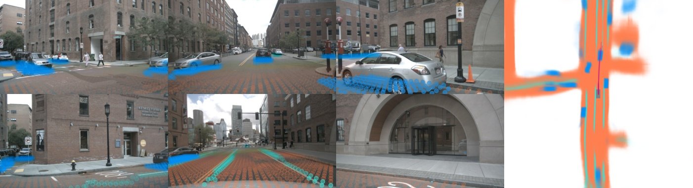
Figure 1: We propose a model that, given multi-view camera data (left), infers semantics directly in the bird’s-eye-view (BEV) coordinate frame (right). We show vehicle segmentation (blue), drivable area (orange), and lane segmentation (green). These BEV predictions are then projected back onto input images (dots on the left).

图 1：给定多视角相机数据（左），模型直接在鸟瞰（BEV）坐标系中推断语义（右）。图中蓝色为车辆分割，橙色为可行驶区域，绿色为车道分割。这些 BEV 预测再投影回输入图像（左侧的点）。

1 Introduction

1 引言

Computer vision algorithms generally take as input an image and output either a prediction that is coordinate-frame agnostic – such as in classification [19, 30, 16, 17] – or a prediction in the same coordinate frame as the input image – such as in object detection, semantic segmentation, or panoptic segmentation [7, 1, 15, 36].

计算机视觉算法通常以一张图像为输入，输出要么与坐标系无关——如分类 [19, 30, 16, 17]——要么与输入图像处于同一坐标系——如目标检测、语义分割或全景分割 [7, 1, 15, 36]。

This paradigm does not match the setting for perception in self-driving out-of-the-box. In self-driving, multiple sensors are given as input, each with a different coordinate frame, and perception models are ultimately tasked with producing predictions in a new coordinate frame – the frame of the ego car – for consumption by the downstream planner, as shown in Fig. 2.

这一范式并不能开箱即用地匹配自动驾驶感知设定。自动驾驶中输入是多个传感器，各自坐标系不同，而感知模型最终要在新的坐标系——自车坐标系——中给出预测，供下游规划器使用，如图 2 所示。

There are many simple, practical strategies for extending the single-image paradigm to the multi-view setting. For instance, for the problem of 3D object detection from $n$ cameras, one can apply a single-image detector to all input images individually, then rotate and translate each detection into the ego frame according to the intrinsics and extrinsics of the camera in which the object was detected. This extension of the single-view paradigm to the multi-view setting has three valuable symmetries baked into it:

把单图范式扩到多视角，有许多简单实用的做法。例如，从 $n$ 路相机做三维目标检测时，可对每张输入图单独跑单图检测器，再按检测到物体的那台相机的内外参，把每个检测旋到并平移到自车坐标系。这种单视角到多视角的扩展，内嵌了三种有价值的对称性：

1. Translation equivariance – If pixel coordinates within an image are all shifted, the output will shift by the same amount. Fully convolutional single-image object detectors roughly have this property and the multi-view extension inherits this property from them [11] [6].

1. 平移等变性——若图像内像素坐标整体平移，输出也会同等平移。全卷积单图目标检测器大致具备该性质，多视角扩展从它们继承了这一性质 [11] [6]。

2. Permutation invariance – the final output does not depend on a specific ordering of the $n$ cameras.

2. 置换不变性——最终输出不依赖 $n$ 路相机的特定排序。

3. Ego-frame isometry equivariance – the same objects will be detected in a given image no matter where the camera that captured the image was located relative to the ego car. An equivalent way to state this property is that the definition of the ego-frame can be rotated/translated and the output will rotate/translate with it.

3. 自车坐标系等距等变性——无论拍到该图的相机相对自车如何放置，同一图像中都会检测到相同物体。等价表述是：自车坐标系的定义可旋转/平移，输出随之旋转/平移。

The downside of the simple approach above is that using post-processed detections from the single-image detector prevents one from differentiating from predictions made in the ego frame all the way back to the sensor inputs. As a result, the model cannot learn in a data-driven way what the best way is to fuse information across cameras. It also means backpropagation cannot be used to automatically improve the perception system using feedback from the downstream planner.

上述简单做法的缺点是：只用单图检测器后处理过的检测结果，无法从自车坐标系中的预测一路可微地回传到传感器输入。因此模型无法以数据驱动方式学习跨相机融合的最佳方式；也无法用反向传播，根据下游规划器的反馈自动改进感知系统。

We propose a model named “Lift-Splat” that preserves the 3 symmetries identified above by design while also being end-to-end differentiable. In Section 3, we explain how our model “lifts” images into 3D by generating a frustum-shaped point cloud of contextual features, “splats” all frustums onto a reference plane as is convenient for the downstream task of motion planning. In Section 3.3, we propose a method for “shooting” proposal trajectories into this reference plane for interpretable end-to-end motion planning. In Section 4, we identify implementation details for training lift-splat models efficiently on full camera rigs. We present empirical evidence in Sec 5 that our model learns an effective mechanism for fusing information from a distribution of possible inputs.

我们提出名为「Lift-Splat」的模型：在设计上保留上述三种对称性，同时又端到端可微。第 3 节说明模型如何通过生成锥体状上下文特征点云把图像「抬升」到三维，再把所有视锥「泼溅」到便于下游运动规划的参考平面上。第 3.3 节提出把提案轨迹「射出」到该参考平面、用于可解释端到端运动规划的方法。第 4 节给出在完整相机配置上高效训练 lift-splat 模型的实现细节。第 5 节给出经验证据：模型能学到对一类可能输入分布有效的融合机制。

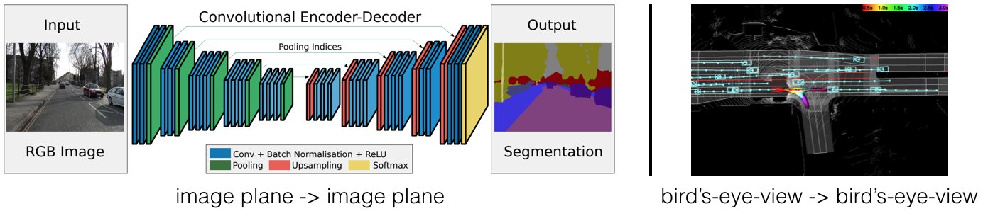
Figure 2: (left, from SegNet [1]) Traditionally, computer vision tasks such as semantic segmentation involve making predictions in the same coordinate frame as the input image. (right, from Neural Motion Planner [41]) In contrast, planning for self-driving generally operates in the bird’s-eye-view frame. Our model directly makes predictions in a given bird’s-eye-view frame for end-to-end planning from multi-view images.

图 2：（左，来自 SegNet [1]）传统计算机视觉任务如语义分割，在与输入图像相同的坐标系中做预测。（右，来自 Neural Motion Planner [41]）相比之下，自动驾驶规划通常在鸟瞰坐标系中运行。我们的模型直接在给定鸟瞰坐标系中做预测，从而从多视角图像端到端规划。

2 Related Work

2 相关工作

Our approach for learning cohesive representations from image data from multiple cameras builds on recent work in sensor fusion and monocular object detection. Large scale multi-modal datasets from Nutonomy [2], Lyft [13], Waymo [35], and Argo [3], have recently made full representation learning of the entire $360^{\circ}$ scene local to the ego vehicle conditioned exclusively on camera input a possibility. We explore that possibility with our Lift-Splat architecture.

我们从多相机图像学习连贯表示的方法，建立在传感器融合与单目目标检测近期工作之上。Nutonomy [2]、Lyft [13]、Waymo [35]、Argo [3] 等大规模多模态数据集，使仅以相机输入、对自车周围整圈 $360^{\circ}$ 场景做完整表示学习成为可能。我们用 Lift-Splat 架构探索这一可能。

2.1 Monocular Object Detection

2.1 单目目标检测

Monocular object detectors are defined by how they model the transformation from the image plane to a given 3-dimensional reference frame. A standard technique is to apply a mature 2D object detector in the image plane and then train a second network to regress 2D boxes into 3D boxes [12, 26, 31, 27]. The current state-of-the-art 3D object detector on the nuScenes benchmark [31] uses an architecture that trains a standard 2d detector to also predict depth using a loss that seeks to disentangle error due to incorrect depth from error due to incorrect bounding boxes. These approaches achieve great performance on 3D object detection benchmarks because detection in the image plane factors out the fundamental cloud of ambiguity that shrouds monocular depth prediction.

单目目标检测器由它们如何建模从图像平面到给定三维参考系的变换来定义。标准做法是在图像平面上跑成熟的二维检测器，再训练第二个网络把二维框回归成三维框 [12, 26, 31, 27]。nuScenes 基准上当前最强的三维检测器 [31] 采用的结构，是让标准二维检测器同时预测深度，并用一项损失把错误深度造成的误差与错误框造成的误差解耦。这类方法在三维检测基准上表现很好，因为图像平面上的检测把单目深度预测固有的那团模糊性「提出」去了。

An approach with recent empirical success is to separately train one network to do monocular depth prediction and another to do bird’s-eye-view detection separately [39] [40]. These approaches go by the name of “pseudolidar”. The intuitive reason for the empirical success of pseudolidar is that pseudolidar enables training a bird’s-eye-view network that operates in the coordinate frame where the detections are ultimately evaluated and where, relative to the image plane, euclidean distance is more meaningful.

近期经验上成功的一类做法，是分别训练一个网络做单目深度预测、另一个做鸟瞰检测 [39] [40]，统称「伪激光雷达」（pseudolidar）。其直观理由是：伪激光雷达让人可以在最终评估检测、且相对图像平面欧氏距离更有意义的坐标系里，训练鸟瞰网络。

A third category of monocular object detectors uses 3-dimensional object primitives that acquire features based on their projection onto all available cameras. Mono3D [4] achieved state of the art monocular object detection on KITTI by generating 3-dimensional proposals on a ground plane that are scored by projecting onto available images. Orthographic Feature Transform [29] builds on Mono3D by projecting a fixed cube of voxels onto images to collect features and then training a second “BEV” CNN to detect in 3D conditioned on the features in the voxels. A potential performance bottleneck of these models that our model addresses is that a pixel contributes the same feature to every voxel independent of the depth of the object at that pixel.

第三类单目检测器使用三维物体基元，按它们投影到所有可用相机上收集特征。Mono3D [4] 在地面上生成三维提案，再投影到可用图像上打分，从而在 KITTI 上达到当时最强单目检测。Orthographic Feature Transform [29] 在 Mono3D 之上，把固定体素立方投影到图像上收集特征，再训练第二个「BEV」CNN 在体素特征上做三维检测。这类模型的一个潜在性能瓶颈——也是我们要解决的——是：无论该像素处物体深度如何，同一像素对每个体素贡献相同特征。

2.2 Inference in the Bird’s-Eye-View Frame

2.2 在鸟瞰坐标系中推理

Models that use extrinsics and intrinsics in order to perform inference directly in the bird’s-eye-view frame have received a large amount of interest recently. MonoLayout [21] performs bird’s-eye-view inference from a single image and uses an adversarial loss to encourage the model to inpaint plausible hidden objects. In concurrent work, Pyramid Occupancy Networks [28] proposes a transformer architecture that converts image representations into bird’s-eye-view representations. FISHING Net [9] - also concurrent work - proposes a multi-view architecture that both segments objects in the current timestep and performs future prediction. We show that our model outperforms prior work empirically in Section 5. These architectures, as well as ours, use data structures similar to “multi-plane” images from the machine learning graphics community [34, 32, 38, 20].

利用内外参直接在鸟瞰坐标系推理的模型近来很受关注。MonoLayout [21] 从单图做鸟瞰推理，并用对抗损失鼓励模型补全合理的被遮挡物体。同期工作 Pyramid Occupancy Networks [28] 提出把图像表示转成鸟瞰表示的 Transformer 结构。FISHING Net [9]——亦为同期工作——提出多视角架构，既分割当前时刻物体，也做未来预测。我们在第 5 节表明本模型在经验上优于先前工作。这些结构以及我们的结构，都使用了与机器学习图形学社区「多平面」图像类似的数据结构 [34, 32, 38, 20]。

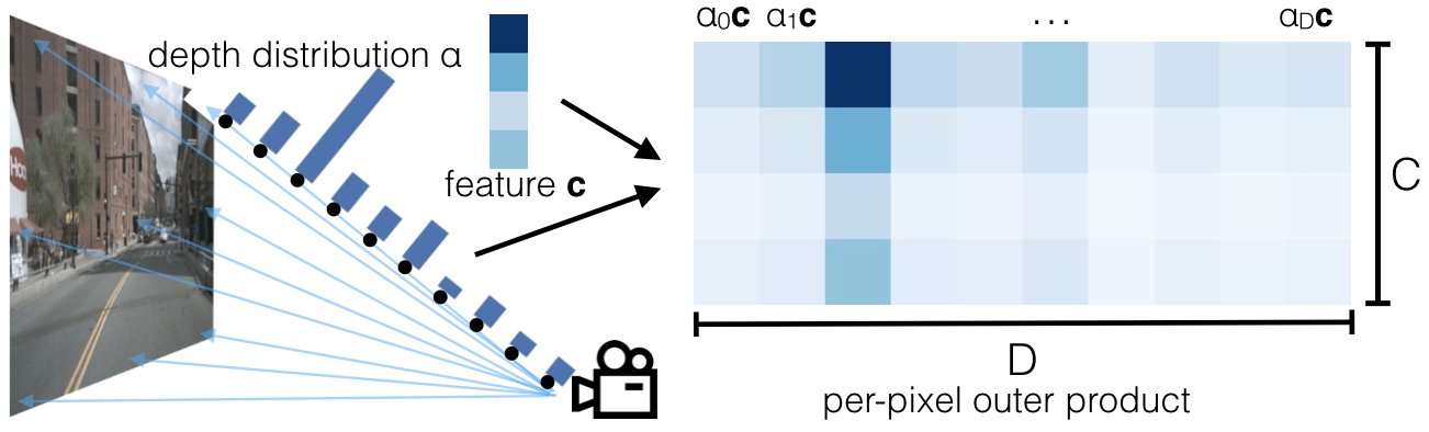
Figure 3: We visualize the “lift” step of our model. For each pixel, we predict a categorical distribution over depth $\alpha\in\triangle^{D-1}$ (left) and a context vector $\mathbf{c}\in\mathbb{R}^{C}$ (top left). Features at each point along the ray are determined by the outer product of $\alpha$ and $\mathbf{c}$ (right).

图 3：可视化模型的「抬升」步骤。对每个像素，预测深度上的类别分布 $\alpha\in\triangle^{D-1}$（左）与上下文向量 $\mathbf{c}\in\mathbb{R}^{C}$（左上）。沿射线各点的特征由 $\alpha$ 与 $\mathbf{c}$ 的外积决定（右）。

3 Method

3 方法

In this section, we present our approach for learning bird’s-eye-view representations of scenes from image data captured by an arbitrary camera rig. We design our model such that it respects the symmetries identified in Section 1.

本节给出从任意相机配置拍摄的图像学习场景鸟瞰表示的方法。模型设计遵守第 1 节指出的对称性。

Formally, we are given $n$ images $\{\mathbf{X}_{k}\in\mathbb{R}^{3\times H\times W}\}_{n}$ each with an extrinsic matrix $\mathbf{E}_{k}\in\mathbb{R}^{3\times 4}$ and an intrinsic matrix $\mathbf{I}_{k}\in\mathbb{R}^{3\times 3}$, and we seek to find a rasterized representation of the scene in the BEV coordinate frame $\mathbf{y}\in\mathbb{R}^{C\times X\times Y}$. The extrinsic and intrinsic matrices together define the mapping from reference coordinates $(x,y,z)$ to local pixel coordinates $(h,w,d)$ for each of the $n$ cameras. We do not require access to any depth sensor during training or testing.

形式化地，给定 $n$ 张图像 $\{\mathbf{X}_{k}\in\mathbb{R}^{3\times H\times W}\}_{n}$，各自外参 $\mathbf{E}_{k}\in\mathbb{R}^{3\times 4}$ 与内参 $\mathbf{I}_{k}\in\mathbb{R}^{3\times 3}$，我们要在 BEV 坐标系中求场景的栅格化表示 $\mathbf{y}\in\mathbb{R}^{C\times X\times Y}$。内外参共同定义了从参考坐标 $(x,y,z)$ 到各相机局部像素坐标 $(h,w,d)$ 的映射。训练与测试都不需要深度传感器。

3.1 Lift: Latent Depth Distribution

3.1 Lift：隐深度分布

The first stage of our model operates on each image in the camera rig in isolation. The purpose of this stage is to “lift” each image from a local 2-dimensional coordinate system to a 3-dimensional frame that is shared across all cameras.

模型第一阶段对相机配置中的每张图像单独处理。目的是把每张图像从局部二维坐标系「抬升」到所有相机共享的三维坐标系。

The challenge of monocular sensor fusion is that we require depth to transform into reference frame coordinates but the “depth” associated to each pixel is inherently ambiguous. Our proposed solution is to generate representations at all possible depths for each pixel.

单目传感器融合的难点在于：变换到参考系坐标需要深度，但每个像素关联的「深度」本质上模糊。我们的方案是：对每个像素在所有可能深度上生成表示。

Let $\mathbf{X}\in\mathbb{R}^{3\times H\times W}$ be an image with extrinsics $\mathbf{E}$ and intrinsics $\mathbf{I}$, and let $p$ be a pixel in the image with image coordinates $(h,w)$. We associate $|D|$ points $\{(h,w,d)\in\mathbb{R}^{3}\mid d\in D\}$ to each pixel where $D$ is a set of discrete depths, for instance defined by $\{d_{0}+\Delta,...,d_{0}+|D|\Delta\}$. Note that there are no learnable parameters in this transformation. We simply create a large point cloud for a given image of size $D\cdot H\cdot W$. This structure is equivalent to what the multi-view synthesis community [38, 32] has called a multi-plane image except in our case the features in each plane are abstract vectors instead of $(r,g,b,\alpha)$ values.

设 $\mathbf{X}\in\mathbb{R}^{3\times H\times W}$ 为带外参 $\mathbf{E}$、内参 $\mathbf{I}$ 的图像，$p$ 为图像坐标 $(h,w)$ 的像素。我们给每个像素关联 $|D|$ 个点 $\{(h,w,d)\in\mathbb{R}^{3}\mid d\in D\}$，其中 $D$ 是离散深度集合，例如 $\{d_{0}+\Delta,...,d_{0}+|D|\Delta\}$。注意该变换没有可学习参数。我们对给定图像简单生成大小为 $D\cdot H\cdot W$ 的大点云。该结构等价于多视角合成社区 [38, 32] 所称的多平面图像，只是我们每层平面上的特征是抽象向量，而非 $(r,g,b,\alpha)$ 值。

The context vector for each point in the point cloud is parameterized to match a notion of attention and discrete depth inference. At pixel $p$, the network predicts a context $\mathbf{c}\in\mathbb{R}^{C}$ and a distribution over depth $\alpha\in\triangle^{|D|-1}$ for every pixel. The feature $\mathbf{c}_{d}\in\mathbb{R}^{C}$ associated to point $p_{d}$ is then defined as the context vector for pixel $p$ scaled by $\alpha_{d}$:

点云中每点的上下文向量按注意力与离散深度推断的直觉参数化。在像素 $p$，网络预测上下文 $\mathbf{c}\in\mathbb{R}^{C}$ 以及每个像素上的深度分布 $\alpha\in\triangle^{|D|-1}$。与点 $p_{d}$ 关联的特征 $\mathbf{c}_{d}\in\mathbb{R}^{C}$ 定义为像素 $p$ 的上下文向量按 $\alpha_{d}$ 缩放：

$$\displaystyle\mathbf{c}_{d}=\alpha_{d}\mathbf{c}. \tag{1}$$

Note that if our network were to predict a one-hot vector for $\alpha$, context at the point $p_{d}$ would be non-zero exclusively for a single depth $d^{*}$ as in pseudolidar [39]. If the network predicts a uniform distribution over depth, the network would predict the same representation for each point $p_{d}$ assigned to pixel $p$ independent of depth as in OFT [29]. Our network is therefore in theory capable of choosing between placing context from the image in a specific location of the bird’s-eye-view representation versus spreading the context across the entire ray of space, for instance if the depth is ambiguous.

注意：若网络把 $\alpha$ 预测成 one-hot，则点 $p_{d}$ 处的上下文仅在单一深度 $d^{*}$ 非零，如同伪激光雷达 [39]。若网络预测深度上的均匀分布，则对赋给像素 $p$ 的每个点 $p_{d}$，网络会给出与深度无关的相同表示，如同 OFT [29]。因此我们的网络原则上能在「把图像上下文放到鸟瞰表示的特定位置」与「把上下文沿整条射线铺开」（例如深度模糊时）之间做选择。

In summary, ideally, we would like to generate a function $g_{c}:(x,y,z)\in\mathbb{R}^{3}\rightarrow c\in\mathbb{R}^{C}$ for each image that can be queried at any spatial location and return a context vector. To take advantage of discrete convolutions, we choose to discretize space. For cameras, the volume of space visible to the camera corresponds to a frustum. A visual is provided in Figure 3.

总之，理想情况下我们希望为每张图像生成可在任意空间位置查询并返回上下文向量的函数 $g_{c}:(x,y,z)\in\mathbb{R}^{3}\rightarrow c\in\mathbb{R}^{C}$。为利用离散卷积，我们选择离散化空间。对相机而言，可见空间体积对应一个视锥。可视化见图 3。

3.2 Splat: Pillar Pooling

3.2 Splat：柱体池化

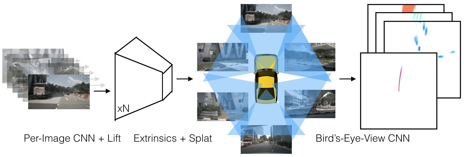
Figure 4: Lift-Splat-Shoot Outline Our model takes as input $n$ images (left) and their corresponding extrinsic and intrinsic parameters. In the “lift” step, a frustum-shaped point cloud is generated for each individual image (center-left). The extrinsics and intrinsics are then used to splat each frustum onto the bird’s-eye-view plane (center-right). Finally, a bird’s-eye-view CNN processes the bird’s-eye-view representation for BEV semantic segmentation or planning (right).

图 4：Lift-Splat-Shoot 概览。模型以 $n$ 张图像（左）及其对应内外参为输入。「抬升」步骤为每张图生成锥体状点云（中左）。再用内外参把各视锥泼溅到鸟瞰平面（中右）。最后，鸟瞰 CNN 处理该鸟瞰表示，用于 BEV 语义分割或规划（右）。

We follow the pointpillars [18] architecture to convert the large point cloud output by the “lift” step. “Pillars” are voxels with infinite height. We assign every point to its nearest pillar and perform sum pooling to create a $C\times H\times W$ tensor that can be processed by a standard CNN for bird’s-eye-view inference. The overall lift-splat architecture is outlined in Figure 4.

我们沿用 PointPillars [18] 架构，把「抬升」输出的大点云转换。「柱体」（pillars）是高度无限的体素。我们把每个点赋给最近柱体，做 sum pooling，得到可由标准 CNN 做鸟瞰推理的 $C\times H\times W$ 张量。整体 lift-splat 结构见图 4。

Just as OFT [29] uses integral images to speed up their pooling step, we apply an analagous technique to speed up sum pooling. Efficiency is crucial for training our model given the size of the point clouds generated. Instead of padding each pillar then performing sum pooling, we avoid padding by using packing and leveraging a “cumsum trick” for sum pooling. This operation has an analytic gradient that can be calculated efficiently to speed up autograd as explained in subsection 4.2.

正如 OFT [29] 用积分图加速池化，我们对 sum pooling 采用类似技巧。鉴于生成的点云规模，效率对训练至关重要。我们不给每个柱体 padding 再 sum pooling，而是用 packing，并借助「cumsum 技巧」做 sum pooling。该运算有可高效计算的解析梯度，以加速 autograd，见第 4.2 小节。

3.3 Shoot: Motion Planning

3.3 Shoot：运动规划

Key aspect of our Lift-Splat model is that it enables end-to-end cost map learning for motion planning from camera-only input. At test time, planning using the inferred cost map can be achieved by “shooting” different trajectories, scoring their cost, then acting according to lowest cost trajectory [25]. In Sec 5.6, we probe the ability of our model to enable end-to-end interpretable motion planning and compare its performance to lidar-based end-to-end neural motion planners.

Lift-Splat 模型的关键一点是：它支持仅从相机输入端到端学习规划用代价图。测试时，用推断出的代价图规划，可通过「射出」不同轨迹、打分其代价，再按最低代价轨迹行动 [25]。第 5.6 节探测模型支撑端到端可解释运动规划的能力，并与基于激光雷达的端到端神经运动规划器比较。

We frame “planning” as predicting a distribution over $K$ template trajectories for the ego vehicle

我们把「规划」表述为：在自车的 $K$ 条模板轨迹上预测分布

$$\mathcal{T}=\{\tau_{i}\}_{K}=\{\{x_{j},y_{j},t_{j}\}_{T}\}_{K}$$

conditioned on sensor observations $p(\tau|o)$. Our approach is inspired by the recently proposed Neural Motion Planner (NMP) [41], an architecture that conditions on point clouds and high-definition maps to generate a cost-volume that can be used to score proposed trajectories.

以传感器观测为条件 $p(\tau|o)$。方法受近期提出的 Neural Motion Planner (NMP) [41] 启发：该结构以点云与高精地图为条件，生成可用于给提案轨迹打分的代价体。

Instead of the hard-margin loss proposed in NMP, we frame planning as classification over a set of $K$ template trajectories. To leverage the cost-volume nature of the planning problem, we enforce the distribution over $K$ template trajectories to take the following form

我们不用 NMP 提出的硬间隔损失，而把规划表述为在 $K$ 条模板轨迹上的分类。为利用规划问题的代价体本质，我们强制 $K$ 条模板轨迹上的分布取如下形式

$$\displaystyle p(\tau_{i}|o)=\frac{\exp\left(-\sum\limits_{x_{i},y_{i}\in\tau_{i}}c_{o}(x_{i},y_{i})\right)}{\sum\limits_{\tau\in\mathcal{T}}\exp\left(-\sum\limits_{x_{i},y_{i}\in\tau}c_{o}(x_{i},y_{i})\right)} \tag{2}$$

where $c_{o}(x,y)$ is defined by indexing into the cost map predicted given observations $o$ at location $x,y$ and can therefore be trained end-to-end from data by optimizing for the log probability of expert trajectories. For labels, given a ground-truth trajectory, we compute the nearest neighbor in L2 distance to the template trajectories $\mathcal{T}$ then train with the cross entropy loss. This definition of $p(\tau_{i}|o)$ enables us to learn an interpretable spatial cost function without defining a hard-margin loss as in NMP [41].

其中 $c_{o}(x,y)$ 由在观测 $o$ 下预测的代价图在位置 $x,y$ 索引得到，因而可通过优化专家轨迹的对数概率从数据端到端训练。标签方面，给定真实轨迹，我们在模板轨迹 $\mathcal{T}$ 中按 L2 距离取最近邻，再用交叉熵训练。该 $p(\tau_{i}|o)$ 定义使我们能学到可解释的空间代价函数，而无需像 NMP [41] 那样定义硬间隔损失。

In practice, we determine the set of template trajectories by running K-Means on a large number of expert trajectories. The set of template trajectories used for “shooting” onto the cost map that we use in our experiments are visualized in Figure 5.

实践中，模板轨迹集合通过对大量专家轨迹跑 K-Means 得到。实验中用于「射出」到代价图的模板轨迹集合见图 5。

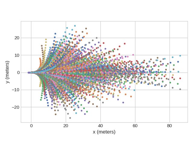
Figure 5: We visualize the 1K trajectory templates that we “shoot” onto our cost map during training and testing. During training, the cost of each template trajectory is computed and interpreted as a 1K-dimensional Boltzman distribution over the templates. During testing, we choose the argmax of this distribution and act according to the chosen template.

图 5：可视化训练与测试时「射出」到代价图上的 1K 条轨迹模板。训练时计算每条模板轨迹的代价，并解释为模板上的 1K 维 Boltzmann 分布。测试时取该分布的 argmax，并按所选模板行动。

4 Implementation

4 实现

4.1 Architecture Details

4.1 架构细节

The neural architecture of our model is similar to OFT [29]. As in OFT, our model has two large network backbones. One of the backbones operates on each image individually in order to featurize the point cloud generated from each image. The other backbone operates on the point cloud once it is splatted into pillars in the reference frame. The two networks are joined by our lift-splat layer as defined in Section 3 and visualize in Figure 4.

模型的神经结构与 OFT [29] 类似。与 OFT 一样，我们有两个大型网络主干。一个主干对每张图像单独运行，以为每张图生成的点云赋特征；另一个主干在点云泼溅成参考系中的柱体之后运行。两个网络由第 3 节定义、图 4 所示的 lift-splat 层相连。

For the network that operates on each image in isolation, we leverage layers from an EfficientNet-B0 [37] pretrained on Imagenet [30] in all experiments for all models including baselines. EfficientNets are network architectures found by exhaustive architecture search in a resource limited regime with depth, width, and resolution scaled up proportionally. We find that they enable higher performance relative to ResNet-18/34/50 [8] across all models with a minor inconvenience of requiring more optimization steps to converge.

对单独处理每张图像的网络，全部实验（含基线）均使用在 ImageNet [30] 上预训练的 EfficientNet-B0 [37] 层。EfficientNet 是在资源受限设定下经穷尽结构搜索、并按深度、宽度与分辨率成比例放大得到的。我们发现相对 ResNet-18/34/50 [8]，它们在所有模型上带来更高性能，代价是收敛需要更多优化步数，略有不便。

For our bird’s-eye-view network, we use a combination of ResNet blocks similar to PointPillars [18]. Specifically, after a convolution with kernel 7 and stride 2 followed by batchnorm [10] and ReLU [22], we pass through the first 3 meta-layers of ResNet-18 to get 3 bird’s-eye-view representations at different resolutions $x_{1},x_{2},x_{3}$. We then upsample $x_{3}$ by a scale factor of 4, concatenate with $x_{1}$, apply a resnet block, and finally upsample by 2 to return to the resolution of the original input bird’s-eye-view pseudo image. We count 14.3M trainable parameters in our final network.

鸟瞰网络方面，我们使用与 PointPillars [18] 类似的 ResNet 块组合。具体地，先做核为 7、步长为 2 的卷积，接 batchnorm [10] 与 ReLU [22]，再经过 ResNet-18 的前 3 个 meta-layer，得到不同分辨率的三个鸟瞰表示 $x_{1},x_{2},x_{3}$。然后将 $x_{3}$ 上采样 4 倍，与 $x_{1}$ 拼接，过一个 resnet 块，最后上采样 2 倍回到原始输入鸟瞰伪图像分辨率。最终网络可训练参数约 14.3M。

There are several hyper-parameters that determine the “resolution” of our model. First, there is the size of the input images $H\times W$. In all experiments below, we resize and crop input images to size $128\times 352$ and adjust extrinsics and intrinsics accordingly. Another important hyperparameter of network is the size the resolution of the bird’s-eye-view grid $X\times Y$. In our experiments, we set bins in both $x$ and $y$ from -50 meters to 50 meters with cells of size 0.5 meters $\times$ 0.5 meters. The resultant grid is therefore $200\times 200$. Finally, there’s the choice of $D$ that determines the resolution of depth predicted by the network. We restrict $D$ between 4.0 meters and 45.0 meters spaced by 1.0 meters. With these hyper-parameters and architectural design choices, the forward pass of the model runs at 35 hz on a Titan V GPU.

有若干超参数决定模型「分辨率」。首先是输入图像尺寸 $H\times W$。下述全部实验中，我们将输入图 resize 并裁到 $128\times 352$，并相应调整内外参。另一重要超参数是鸟瞰网格分辨率 $X\times Y$。实验中，$x$ 与 $y$ 方向的 bin 均从 -50 米到 50 米，格子大小为 0.5 米 $\times$ 0.5 米，因而网格为 $200\times 200$。最后是决定网络深度预测分辨率的 $D$。我们将 $D$ 限制在 4.0 米到 45.0 米、间隔 1.0 米。在这些超参数与结构选择下，模型前向在 Titan V GPU 上跑到 35 Hz。

4.2 Frustum Pooling Cumulative Sum Trick

4.2 视锥池化累加和技巧

Training efficiency is critical for learning from data from an entire sensor rig. We choose sum pooling across pillars in Section 3 as opposed to max pooling because our “cumulative sum” trick saves us from excessive memory usage due to padding. The “cumulative sum trick” is the observation that sum pooling can be performed by sorting all points according to bin id, performing a cumulative sum over all features, then subtracting the cumulative sum values at the boundaries of the bin sections. Instead of relying on autograd to backprop through all three steps, the analytic gradient for the module as a whole can be derived, speeding up training by 2x. We call the layer “Frustum Pooling” because it handles converting the frustums produced by $n$ images into a fixed dimensional $C\times H\times W$ tensor independent of the number of cameras $n$. Code can be found on our project page.

从整套传感器配置的数据学习时，训练效率至关重要。第 3 节我们选柱体上的 sum pooling 而非 max pooling，因为「累加和」技巧可避免 padding 带来的过度显存占用。「累加和技巧」的观察是：sum pooling 可通过按 bin id 排序所有点、对全部特征做累加和，再在 bin 区段边界处减去累加和来完成。我们不依赖 autograd 回传全部三步，而是推导整模块的解析梯度，使训练加速约 2 倍。我们称该层为「Frustum Pooling」，因为它负责把 $n$ 张图像产生的视锥变成与相机数 $n$ 无关的固定维 $C\times H\times W$ 张量。代码见项目页。

5 Experiments and Results

5 实验与结果

We use the nuScenes [2] and Lyft Level 5 [13] datasets to evaluate our approach. nuScenes is a large dataset of point cloud data and image data from 1k scenes, each of 20 seconds in length. The camera rig in both datasets is comprised of 6 cameras which roughly point in the forward, front-left, front-right, back-left, back-right, and back directions. In all datasets, there is a small overlap between the fields-of-view of the cameras. The extrinsic and intrinsic parameters of the cameras shift throughout both datasets. Since our model conditions on the camera calibration, it is able to handle these shifts.

我们用 nuScenes [2] 与 Lyft Level 5 [13] 评估方法。nuScenes 是含点云与图像的大规模数据集，共 1k 个场景，每个长 20 秒。两数据集的相机配置均由约朝前、前左、前右、后左、后右与后方的 6 路相机组成。各数据集中相机视场有小幅重叠。两数据集中相机内外参都会变化。由于模型以相机标定作为条件，能够处理这些变化。

We define two object-based segmentation tasks and two map-based tasks. For the object segmentation tasks, we obtain ground truth bird’s-eye-view targets by projecting 3D bounding boxes into the bird’s-eye-view plane. Car segmentation on nuScenes refers to all bounding boxes of class vehicle.car and vehicle segmentation on nuScenes refers to all bounding boxes of meta-category vehicle. Car segmentation on Lyft refers to all bounding boxes of class car and vehicle segmentation on nuScenes refers to all bounding boxes with class $\in\{$ car, truck, other_vehicle, bus, bicycle $\}$. For mapping, we use transform map layers from the nuScenes map into the ego frame using the provided 6 DOF localization and rasterize.

我们定义两个基于物体的分割任务与两个基于地图的任务。物体分割任务中，把三维边界框投影到鸟瞰平面得到鸟瞰真值目标。nuScenes 上车分割指 vehicle.car 类全部框，车辆分割指 meta-category vehicle 的全部框。Lyft 上车分割指 car 类全部框；车辆分割指类别属于 $\{$ car, truck, other_vehicle, bus, bicycle $\}$ 的全部框。地图任务中，我们用提供的 6 自由度定位把 nuScenes 地图图层变换到自车系并栅格化。

For all object segmentation tasks, we train with binary cross entropy with positive weight 1.0. For the lane segmentation, we set positive weight to 5.0 and for road segmentation we use positive weight 1.0 [24]. In all cases, we train for 300k steps using Adam [14] with learning rate $1e-3$ and weight decay $1e-7$. We use the PyTorch framework [23].

全部物体分割任务用正样本权重 1.0 的二元交叉熵训练。车道分割正样本权重设为 5.0，道路分割用正样本权重 1.0 [24]。所有情形下，用 Adam [14]、学习率 $1e-3$、权重衰减 $1e-7$ 训练 300k 步。框架为 PyTorch [23]。

The Lyft dataset does not come with a canonical train/val split. We separate 48 of the Lyft scenes for validation to get a validation set of roughly the same size as nuScenes (6048 samples for Lyft, 6019 samples for nuScenes).

Lyft 数据集没有标准 train/val 划分。我们留出 48 个 Lyft 场景做验证，使验证集规模大致与 nuScenes 相当（Lyft 6048 样本，nuScenes 6019 样本）。

5.1 Description of Baselines

5.1 基线说明

Unlike vanilla CNNs, our model comes equipped with 3-dimensional structure at initialization. We show that this structure is crucial for good performance by comparing against a CNN composed of standard modules. We follow an architecture similar to MonoLayout [21] which also trains a CNN to output bird’s-eye-view labels from images only but does not leverage inductive bias in designing the architecture and trains on single cameras only. The architecture has an EfficientNet-B0 backbone that extracts features independently across all images. We concatenate the representations and perform bilinear interpolation to upsample into a $\mathbb{R}^{X\times Y}$ tensor as is output by our model. We design the network such that it has roughly the same number of parameters as our model. The weak performance of this baseline demonstrates how important it is to explicitly bake symmetry 3 from Sec 1 into the model in the multi-view setting.

与普通 CNN 不同，我们的模型在初始化时就带有三维结构。我们通过与由标准模块组成的 CNN 对比，表明该结构对良好性能至关重要。结构类似 MonoLayout [21]：也仅从图像训练 CNN 输出鸟瞰标签，但不在结构设计中利用归纳偏置，且只在单相机上训练。该结构用 EfficientNet-B0 主干在所有图像上独立提特征，拼接表示后再双线性插值上采样到与我们模型输出同形的 $\mathbb{R}^{X\times Y}$ 张量。我们把网络参数量设计得与本模型大致相同。该基线表现疲弱，说明在多视角设定下把第 1 节对称性 3 显式写进模型有多重要。

To show that our model is predicting a useful implicit depth, we compare against our model where the weights of the pretrained CNN are frozen as well as to OFT [29]. We outperform these baselines on all tasks, as shown in Tables 2 and 2. We also outperform concurrent work that benchmarks on the same segmentation tasks [9] [28]. As a result, the architecture is learning both an effective depth distribution as well as effective contextual representations for the downstream task.

为表明模型在预测有用的隐深度，我们还与冻结预训练 CNN 权重的本模型以及 OFT [29] 对比。如表 2 与表 2 所示，我们在全部任务上超过这些基线，也超过在相同分割任务上评测的同期工作 [9] [28]。因此，该结构既学到了有效的深度分布，也为下游任务学到了有效的上下文表示。

5.2 Segmentation

5.2 分割

We demonstrate that our Lift-Splat model is able to learn semantic 3D representations given supervision in the bird’s-eye-view frame. Results on the object segmentation tasks are shown in Table 2, while results on the map segmentation tasks are in Table 2. On all benchmarks, we outperform our baselines. We believe the extent of these gains in performance from implicitly unprojecting into 3D are substantial, especially for object segmentation. We also include reported IOU scores for two concurrent works [9] [28] although both of these papers use different definitions of the bird’s-eye-view grid and a different validation split for the Lyft dataset so a true comparison is not yet possible.

我们表明：在鸟瞰坐标系监督下，Lift-Splat 能学到语义三维表示。物体分割结果见表 2，地图分割见表 2。全部基准上我们都超过基线。我们认为，隐式反投影到三维带来的性能增益幅度相当可观，尤其在物体分割上。我们也列入两项同期工作 [9] [28] 报告的 IOU，但这两篇对鸟瞰网格的定义不同，且 Lyft 验证划分也不同，因而尚不能做真正对齐的比较。

nuScenes Lyft Car Vehicles Car Vehicles CNN 22.78 24.25 30.71 31.91 Frozen Encoder 25.51 26.83 35.28 32.42 OFT 29.72 30.05 39.48 40.43 Lift-Splat (Us) 32.06 32.07 43.09 44.64 PON∗ [28] 24.7 - - - FISHING∗ [9] - 30.0 - 56.0

Drivable Area Lane Boundary CNN 68.96 16.51 Frozen Encoder 61.62 16.95 OFT 71.69 18.07 Lift-Splat (Us) 72.94 19.96 PON∗ [28] 60.4 -

Table 1: Segment. IOU in BEV frame

nuScenes Lyft 车 车辆 车 车辆 CNN 22.78 24.25 30.71 31.91 Frozen Encoder 25.51 26.83 35.28 32.42 OFT 29.72 30.05 39.48 40.43 Lift-Splat（本文） 32.06 32.07 43.09 44.64 PON∗ [28] 24.7 - - - FISHING∗ [9] - 30.0 - 56.0

可行驶区域 车道边界 CNN 68.96 16.51 Frozen Encoder 61.62 16.95 OFT 71.69 18.07 Lift-Splat（本文） 72.94 19.96 PON∗ [28] 60.4 -

表 1：BEV 坐标系下的分割 IOU

5.3 Robustness

5.3 稳健性

Because the bird’s-eye-view CNN learns from data how to fuse information across cameras, we can train the model to be robust to simple noise models that occur in self-driving such as extrinsics being biased or cameras dying. In Figure 6, we verify that by dropping cameras during training, our model handles dropped cameras at better at test time. In fact, the best performing model when all 6 cameras are present is the model that is trained with 1 camera being randomly dropped from every sample during training. We reason that sensor dropout forces the model to learn the correlation between images on different cameras, similar to other variants of dropout [33] [5]. We show on the left of Figure 6 that training the model with noisy extrinsics can lead to better test-time performance. For low amounts of noise at test-time, models that are trained without any noise in the extrinsics perform the best because the BEV CNN can trust the location of the splats with more confidence. For high amounts of extrinsic noise, our model sustains its good performance.

由于鸟瞰 CNN 从数据中学习如何跨相机融合信息，我们可以训练模型对自动驾驶中常见的简单噪声模型稳健，例如外参有偏或相机失效。图 6 验证：训练时丢相机，测试时模型对丢相机处理更好。事实上，当 6 路相机都在时表现最好的模型，是训练时每个样本随机丢掉 1 路相机的那个。我们推断传感器 dropout 迫使模型学习不同相机图像之间的相关，类似于其他 dropout 变体 [33] [5]。图 6 左侧表明，用带噪外参训练可带来更好的测试表现。测试时噪声较小时，外参完全无噪声训练的模型最好，因为 BEV CNN 可以更有把握地信任泼溅位置。外参噪声很大时，我们的模型仍能维持良好表现。

In Figure 7, we measure the “importance” of each camera for the performance of car segmentation on nuScenes. Note that losing cameras on nuScenes implies that certain regions of the region local to the car have no sensor measurements and as a result performance strictly upper bounded by performance with the full sensor rig. Qualitative examples in which the network inpaints due to missing cameras are shown in Figure 8. In this way, we measure the importance of each camera, suggesting where sensor redundancy is more important for safety.

图 7 中，我们度量 nuScenes 上车分割性能下每路相机的「重要性」。注意：丢掉 nuScenes 上的相机会使自车附近某些区域没有任何传感器测量，因而性能严格上界于全传感器配置。因缺相机而由网络补全的定性例子见图 8。由此我们度量各相机重要性，提示安全上何处更需要传感器冗余。

(a) Test Time Extrinsic Noise

（a）测试时外参噪声

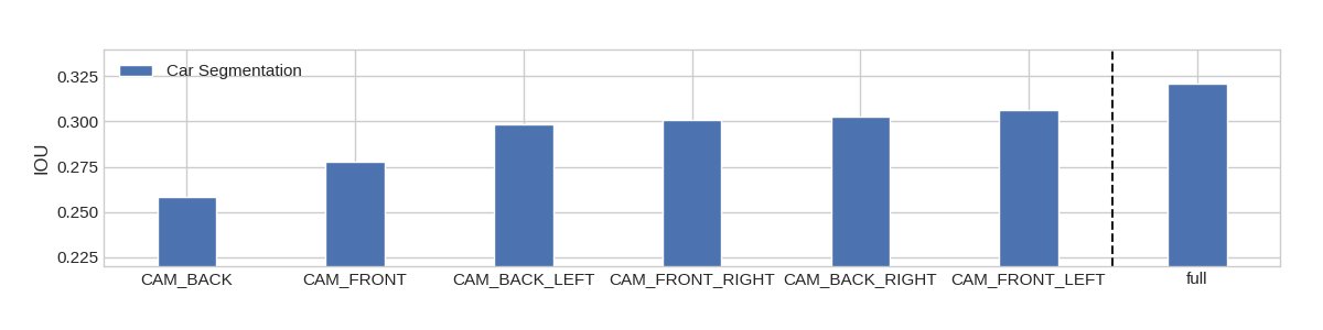
Figure 7: We measure intersection-over-union of car segmentation when each of the cameras is missing. The backwards camera on the nuScenes camera rig has a wider field of view so it is intuitive that losing this camera causes the biggest decrease in performance relative to performance given the full camera rig (labeled “full” on the right).

图 7：度量每路相机缺失时车分割的交并比。nuScenes 相机配置中后向相机视场更宽，因此丢失该相机相对完整配置（右侧标为「full」）造成的性能下降最大，这与直觉一致。

Figure 8: For a single time stamp, we remove each of the cameras and visualize how the loss the cameras effects the prediction of the network. Region covered by the missing camera becomes fuzzier in every case. When the front camera is removed (top middle), the network extrapolates the lane and drivable area in front of the ego and extrapolates the body of a car for which only a corner can be seen in the top right camera.

图 8：在单一时间戳上依次去掉各相机，可视化缺相机如何影响网络预测。被缺相机覆盖的区域在每种情形下都变得更模糊。去掉前向相机时（上中），网络外推出自车前方的车道与可行驶区域，并对外推右上相机中仅能看到一角的车身。

5.4 Zero-Shot Camera Rig Transfer

5.4 零样本相机配置迁移

We now probe the generalization capabilities of Lift-Splat. In our first experiment, we measure performance of our model when only trained on images from a subset of cameras from the nuScenes camera rig but at test time has access to images from the remaining two cameras. In Table 3, we show that the performance of our model for car segmentation improves when additional cameras are available at test time without any retraining.

我们接着探测 Lift-Splat 的泛化能力。第一个实验中，模型只在 nuScenes 相机配置的子集图像上训练，测试时却能用到其余两路相机的图像。表 3 表明：无需重训，测试时增加相机，车分割性能就会提升。

IOU 4 26.53 $4+1_{fl}$ 27.35 $4+1_{bl}$ 27.27 $4+1_{bl}+1_{fl}$ 27.94

Table 3: We train on images from only 4 of the 6 cameras in the nuScenes dataset. We then evaluate with the new cameras ($1_{bl}$ corresponds to the “back left” camera and $1_{fl}$ corresponds to the “front left” camera) and find that the performance of the model strictly increases as we add more sensors unseen during training.

IOU 4 26.53 $4+1_{fl}$ 27.35 $4+1_{bl}$ 27.27 $4+1_{bl}+1_{fl}$ 27.94

表 3：我们仅用 nuScenes 六路相机中的四路图像训练，再在新相机上评估（$1_{bl}$ 为「后左」，$1_{fl}$ 为「前左」），发现随着加入训练未见过的传感器，模型性能严格上升。

We take the above experiment a step farther and probe how well our model generalizes to the Lyft camera rig if it was only trained on nuScenes data. Qualitative results of the transfer are shown in Figure 9 and the benchmark against the generalization of our baselines is shown in Table 4.

我们把上述实验再推进一步：探测只在 nuScenes 上训练的模型，迁移到 Lyft 相机配置时表现如何。迁移的定性结果见图 9，相对基线泛化能力的基准见表 4。

Lyft Car Lyft Vehicle CNN 7.00 8.06 Frozen Encoder 15.08 15.82 OFT 16.25 16.27 Lift-Splat (Us) 21.35 22.59

Table 4: We train the model on nuScenes then evaluate it on Lyft. The Lyft cameras are entirely different from the nuScenes cameras but the model succeeds in generalizing far better than the baselines. Note that our model has widened the gap from the standard benchmark in Tables 2 and 2.

Lyft 车 Lyft 车辆 CNN 7.00 8.06 Frozen Encoder 15.08 15.82 OFT 16.25 16.27 Lift-Splat（本文） 21.35 22.59

表 4：在 nuScenes 上训练再在 Lyft 上评估。Lyft 相机与 nuScenes 完全不同，但模型泛化远好于基线。注意相对表 2 与表 2 的标准基准，本模型拉开的差距更大。

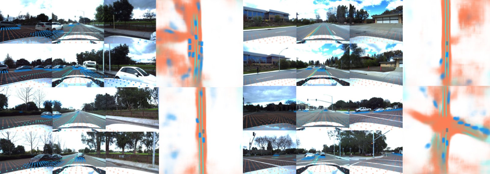
Figure 9: We qualitatively show how our model performs given an entirely new camera rig at test time. Road segmentation is shown in orange, lane segmentation is shown in green, and vehicle segmentation is shown in blue.

图 9：定性展示测试时面对全新相机配置时模型的表现。道路分割为橙，车道分割为绿，车辆分割为蓝。

5.5 Benchmarking Against Oracle Depth

5.5 对照 Oracle 深度

We benchmark our model against the pointpillars [18] architecture which uses ground truth depth from LIDAR point clouds. As shown in Table 5, across all tasks, our architecture performs slightly worse than pointpillars trained with a single scan of LIDAR. However, at least on drivable area segmentation, we note that we approach the performance of LIDAR. In the world in general, not all lanes are visible in a lidar scan. We would like to measure performance in a wider range of environments in the future.

我们与使用激光雷达点云真值深度的 PointPillars [18] 架构对比。如表 5，全部任务上我们的结构略弱于用单帧激光雷达训练的 PointPillars。不过至少在可行驶区域分割上，我们已接近激光雷达表现。现实世界中并非所有车道都能在激光雷达扫描中看见。我们希望未来在更广环境范围上度量性能。

To gain insight into how our model differs from LIDAR, we plot how performance of car segmentation varies with two control variates: distance to the ego vehicle and weather conditions. We determine the weather of a scene from the description string that accompanies every scene token in the nuScenes dataset. The results are shown in Figure 10. We find that performance of our model is much worse than pointpillars on scenes that occur at night as expected. We also find that both models experience roughly linear performance decrease with increased depth.

为洞察模型与激光雷达的差异，我们画出车分割性能随两个控制变量的变化：到自车的距离与天气。天气由 nuScenes 中每个场景 token 附带的描述字符串判定。结果见图 10。我们发现夜间场景上本模型明显弱于 PointPillars，符合预期。两模型随深度增加也大致呈线性性能下降。

nuScenes Lyft Drivable Area Lane Boundary Car Vehicle Car Vehicle Oracle Depth (1 scan) 74.91 25.12 40.26 44.48 74.96 76.16 Oracle Depth ($>1$ scan) 76.96 26.80 45.36 49.51 75.42 76.49 Lift-Splat (Us) 70.81 19.58 32.06 32.07 43.09 44.64

Table 5: When compared to models that use oracle depth from lidar, there is still room for improvement. Video inference from camera rigs is likely necessary to acquire the depth estimates necessary to surpass lidar.

nuScenes Lyft 可行驶区域 车道边界 车 车辆 车 车辆 Oracle 深度（1 帧） 74.91 25.12 40.26 44.48 74.96 76.16 Oracle 深度（$>1$ 帧） 76.96 26.80 45.36 49.51 75.42 76.49 Lift-Splat（本文） 70.81 19.58 32.06 32.07 43.09 44.64

表 5：与使用激光雷达 oracle 深度的模型相比，仍有提升空间。要从相机配置获得足以超越激光雷达的深度估计，很可能需要视频推理。

(a) IOU versus distance

（a）IOU 对距离

5.6 Motion Planning

5.6 运动规划

Finally, we evaluate the capability of our model to perform planning by training the representation output by Lift-Splat to be a cost function. The trajectories that we generate are 5 seconds long spaced by 0.25 seconds. To acquire templates, we fit K-Means for $K=1000$ to all ego trajectories in the training set of nuScenes. At test time, we measure how well the network is able to predict the template that is closest to the ground truth trajectory under the L2 norm. This task is an important experiment for self-driving because the ground truth targets for this experiment are orders of magnitude less expensive to acquire than ground truth 3D bounding boxes. This task is also important for benchmarking the performance of camera-based approaches versus lidar-based approaches because although the ceiling for 3D object detection from camera-only is certainly upper bounded by lidar-only, the optimal planner using camera-only should in principle upper bound the performance of an optimal planner trained from lidar-only.

最后，我们评估把 Lift-Splat 输出的表示训练成代价函数以做规划的能力。生成的轨迹长 5 秒、间隔 0.25 秒。模板通过对 nuScenes 训练集全部自车轨迹拟合 $K=1000$ 的 K-Means 得到。测试时，度量网络预测在 L2 范数下最接近真实轨迹的那条模板的能力。该任务对自动驾驶很重要，因为其真值目标的获取成本比真值三维框低几个数量级。该任务也对标定仅相机相对仅激光雷达的方法重要：尽管仅相机三维检测的天花板一定被仅激光雷达上界，但仅相机的最优规划器原则上应上界于仅从激光雷达训练的最优规划器。

Qualitative results of the planning experiment are shown in Figure 11. The empirical results benchmarked against pointpillars are shown in Table 6. The output trajectories exhibit desirable behavior such as following road boundaries and stopping at crosswalks or behind braking vehicles.

规划实验的定性结果见图 11，相对 PointPillars 的经验结果见表 6。输出轨迹表现出沿道路边界行驶、在人行横道或制动车辆后停下等合意行为。

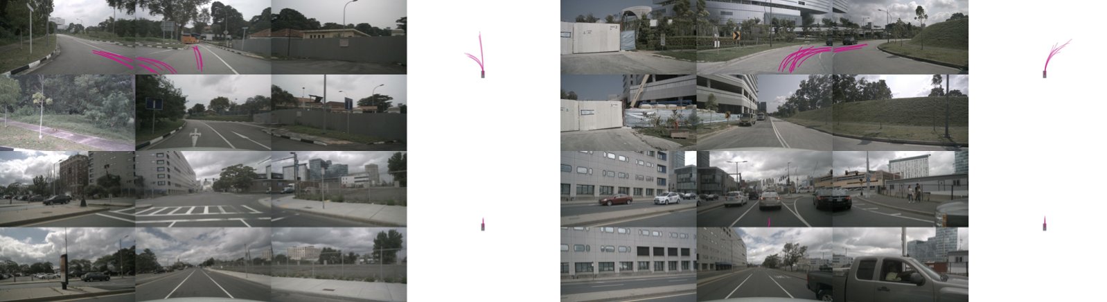
Figure 11: We display the top 10 ranked trajectories out of the 1k templates. Video sequences are provided on our project page. Our model predicts bimodal distributions and curves from observations from a single timestamp. Our model does not have access to the speed of the car so it is compelling that the model predicts low-speed trajectories near crosswalks and brake lights.

图 11：展示 1k 条模板中排名前 10 的轨迹。视频序列见项目页。模型从单时刻观测预测双峰分布与弯道。模型没有车速信息，却能在人行横道与刹车灯附近预测低速轨迹，这一点值得注意。

Top 5 Top 10 Top 20 Lidar (1 scan) 19.27 28.88 41.93 Lidar (10 scans) 24.99 35.39 49.84 Lift-Splat (Us) 15.52 19.94 27.99

Table 6: Since planning is framed as classification among a set of 1K template trajectories, we measure top-5, top-10, and top-20 accuracy. We find that our model is still lagging behind lidar-based approaches in generalization. Qualitative examples of the trajectories output by our model are shown in Fig. 11.

Top 5 Top 10 Top 20 激光雷达（1 帧） 19.27 28.88 41.93 激光雷达（10 帧） 24.99 35.39 49.84 Lift-Splat（本文） 15.52 19.94 27.99

表 6：规划被表述为在 1K 条模板轨迹中分类，故度量 top-5、top-10 与 top-20 准确率。我们发现模型在泛化上仍落后于基于激光雷达的方法。模型输出轨迹的定性例子见图 11。

6 Conclusion

6 结论

In this work, we present an architecture designed to infer bird’s-eye-view representations from arbitrary camera rigs. Our model outperforms baselines on a suite of benchmark segmentation tasks designed to probe the model’s ability to represent semantics in the bird’s-eye-view frame without any access to ground truth depth data at training or test time. We present methods for training our model that make the network robust to simple models of calibration noise. Lastly, we show that the model enables end-to-end motion planning that follows the trajectory shooting paradigm. In order to meet and possibly surpass the performance of similar networks that exclusively use ground truth depth data from pointclouds, future work will need to condition on multiple time steps of images instead of a single time step as we consider in this work.

本文提出一种从任意相机配置推断鸟瞰表示的架构。在一套旨在探测模型能否在训练与测试均无真值深度数据时于鸟瞰坐标系表示语义的分割基准上，本模型超过基线。我们给出使网络对简单标定噪声模型稳健的训练方法。最后表明模型支持按轨迹射出范式做端到端运动规划。若要追平乃至超过仅使用点云真值深度的同类网络，未来工作需要以多时刻图像为条件，而非本文所考虑的单时刻。

References

[1] Badrinarayanan, V., Kendall, A., Cipolla, R.: Segnet: A deep convolutional encoder-decoder architecture for image segmentation. CoRR abs/1511.00561 (2015), http://arxiv.org/abs/1511.00561

[2] Caesar, H., Bankiti, V., Lang, A.H., Vora, S., Liong, V.E., Xu, Q., Krishnan, A., Pan, Y., Baldan, G., Beijbom, O.: nuscenes: A multimodal dataset for autonomous driving. CoRR abs/1903.11027 (2019), http://arxiv.org/abs/1903.11027

[3] Chang, M.F., Ramanan, D., Hays, J., Lambert, J., Sangkloy, P., Singh, J., Bak, S., Hartnett, A., Wang, D., Carr, P., et al.: Argoverse: 3d tracking and forecasting with rich maps. IEEE/CVF Conference on Computer Vision and Pattern Recognition (CVPR) (Jun 2019)

[4] Chen, X., Kundu, K., Zhang, Z., Ma, H., Fidler, S., Urtasun, R.: Monocular 3d object detection for autonomous driving. In: IEEE/CVF Conference on Computer Vision and Pattern Recognition (CVPR). pp. 2147–2156 (06 2016)

[5] Ghiasi, G., Lin, T., Le, Q.V.: Dropblock: A regularization method for convolutional networks. CoRR abs/1810.12890 (2018), http://arxiv.org/abs/1810.12890

[6] Goodfellow, I., Bengio, Y., Courville, A.: Deep Learning. MIT Press (2016), http://www.deeplearningbook.org

[7] He, K., Gkioxari, G., Dollár, P., Girshick, R.B.: Mask R-CNN. CoRR abs/1703.06870 (2017), http://arxiv.org/abs/1703.06870

[8] He, K., Zhang, X., Ren, S., Sun, J.: Deep residual learning for image recognition. CoRR abs/1512.03385 (2015), http://arxiv.org/abs/1512.03385

[9] Hendy, N., Sloan, C., Tian, F., Duan, P., Charchut, N., Xie, Y., Wang, C., Philbin, J.: Fishing net: Future inference of semantic heatmaps in grids (2020)

[10] Ioffe, S., Szegedy, C.: Batch normalization: Accelerating deep network training by reducing internal covariate shift. CoRR abs/1502.03167 (2015), http://arxiv.org/abs/1502.03167

[11] Kayhan, O.S., Gemert, J.C.v.: On translation invariance in cnns: Convolutional layers can exploit absolute spatial location. In: Proceedings of the IEEE/CVF Conference on Computer Vision and Pattern Recognition (CVPR) (June 2020)

[12] Kehl, W., Manhardt, F., Tombari, F., Ilic, S., Navab, N.: SSD-6D: making rgb-based 3d detection and 6d pose estimation great again. CoRR abs/1711.10006 (2017)

[13] Kesten, R., Usman, M., Houston, J., Pandya, T., Nadhamuni, K., Ferreira, A., Yuan, M., Low, B., Jain, A., Ondruska, P., Omari, S., Shah, S., Kulkarni, A., Kazakova, A., Tao, C., Platinsky, L., Jiang, W., Shet, V.: Lyft level 5 av dataset 2019. urlhttps://level5.lyft.com/dataset/ (2019)

[14] Kingma, D.P., Ba, J.: Adam: A method for stochastic optimization. CoRR abs/1412.6980 (2014)

[15] Kirillov, A., He, K., Girshick, R.B., Rother, C., Dollár, P.: Panoptic segmentation. CoRR abs/1801.00868 (2018), http://arxiv.org/abs/1801.00868

[16] Krizhevsky, A.: Learning multiple layers of features from tiny images (2009)

[17] Krizhevsky, A., Sutskever, I., Hinton, G.E.: Imagenet classification with deep convolutional neural networks. In: Pereira, F., Burges, C.J.C., Bottou, L., Weinberger, K.Q. (eds.) Advances in Neural Information Processing Systems 25, pp. 1097–1105. Curran Associates, Inc. (2012), http://papers.nips.cc/paper/4824-imagenet-classification-with-deep-convolutional-neural-networks.pdf

[18] Lang, A.H., Vora, S., Caesar, H., Zhou, L., Yang, J., Beijbom, O.: Pointpillars: Fast encoders for object detection from point clouds. CoRR abs/1812.05784 (2018)

[19] Lecun, Y., Bottou, L., Bengio, Y., Haffner, P.: Gradient-based learning applied to document recognition. In: Proceedings of the IEEE. pp. 2278–2324 (1998)

[20] Lombardi, S., Simon, T., Saragih, J., Schwartz, G., Lehrmann, A., Sheikh, Y.: Neural volumes. ACM Transactions on Graphics 38 (4), 1–14 (Jul 2019). https://doi.org/10.1145/3306346.3323020, http://dx.doi.org/10.1145/3306346.3323020

[21] Mani, K., Daga, S., Garg, S., Shankar, N.S., Jatavallabhula, K.M., Krishna, K.M.: Monolayout: Amodal scene layout from a single image. ArXiv abs/2002.08394 (2020)

[22] Nair, V., Hinton, G.E.: Rectified linear units improve restricted boltzmann machines. In: ICML (2010)

[23] Paszke, A., Gross, S., Massa, F., Lerer, A., Bradbury, J., Chanan, G., Killeen, T., Lin, Z., Gimelshein, N., Antiga, L., Desmaison, A., Köpf, A., Yang, E., DeVito, Z., Raison, M., Tejani, A., Chilamkurthy, S., Steiner, B., Fang, L., Bai, J., Chintala, S.: Pytorch: An imperative style, high-performance deep learning library. In: NeurIPS (2019)

[24] Philion, J.: Fastdraw: Addressing the long tail of lane detection by adapting a sequential prediction network. In: Proceedings of the IEEE/CVF Conference on Computer Vision and Pattern Recognition (CVPR) (June 2019)

[25] Philion, J., Kar, A., Fidler, S.: Learning to evaluate perception models using planner-centric metrics. In: Proceedings of the IEEE/CVF Conference on Computer Vision and Pattern Recognition (CVPR) (June 2020)

[26] Poirson, P., Ammirato, P., Fu, C., Liu, W., Kosecka, J., Berg, A.C.: Fast single shot detection and pose estimation. CoRR abs/1609.05590 (2016)

[27] Qin, Z., Wang, J., Lu, Y.: Monogrnet: A geometric reasoning network for monocular 3d object localization. Proceedings of the AAAI Conference on Artificial Intelligence 33 , 8851–8858 (07 2019). https://doi.org/10.1609/aaai.v33i01.33018851

[28] Roddick, T., Cipolla, R.: Predicting semantic map representations from images using pyramid occupancy networks. In: Proceedings of the IEEE/CVF Conference on Computer Vision and Pattern Recognition (CVPR) (June 2020)

[29] Roddick, T., Kendall, A., Cipolla, R.: Orthographic feature transform for monocular 3d object detection. CoRR abs/1811.08188 (2018)

[30] Russakovsky, O., Deng, J., Su, H., Krause, J., Satheesh, S., Ma, S., Huang, Z., Karpathy, A., Khosla, A., Bernstein, M., Berg, A.C., Fei-Fei, L.: Imagenet large scale visual recognition challenge (2014)

[31] Simonelli, A., Bulò, S.R., Porzi, L., López-Antequera, M., Kontschieder, P.: Disentangling monocular 3d object detection. CoRR abs/1905.12365 (2019)

[32] Srinivasan, P.P., Mildenhall, B., Tancik, M., Barron, J.T., Tucker, R., Snavely, N.: Lighthouse: Predicting lighting volumes for spatially-coherent illumination (2020)

[33] Srivastava, N., Hinton, G., Krizhevsky, A., Sutskever, I., Salakhutdinov, R.: Dropout: A simple way to prevent neural networks from overfitting. Journal of Machine Learning Research 15 , 1929–1958 (2014)

[34] Su, H., Jampani, V., Sun, D., Maji, S., Kalogerakis, E., Yang, M., Kautz, J.: Splatnet: Sparse lattice networks for point cloud processing. CoRR abs/1802.08275 (2018), http://arxiv.org/abs/1802.08275

[35] Sun, P., Kretzschmar, H., Dotiwalla, X., Chouard, A., Patnaik, V., Tsui, P., Guo, J., Zhou, Y., Chai, Y., Caine, B., Vasudevan, V., Han, W., Ngiam, J., Zhao, H., Timofeev, A., Ettinger, S., Krivokon, M., Gao, A., Joshi, A., Zhang, Y., Shlens, J., Chen, Z., Anguelov, D.: Scalability in perception for autonomous driving: Waymo open dataset (2019)

[36] Takikawa, T., Acuna, D., Jampani, V., Fidler, S.: Gated-scnn: Gated shape cnns for semantic segmentation. In: Proceedings of the IEEE/CVF International Conference on Computer Vision (ICCV) (October 2019)

[37] Tan, M., Le, Q.V.: Efficientnet: Rethinking model scaling for convolutional neural networks. CoRR abs/1905.11946 (2019), http://arxiv.org/abs/1905.11946

[38] Tucker, R., Snavely, N.: Single-view view synthesis with multiplane images (2020)

[39] Wang, Y., Chao, W., Garg, D., Hariharan, B., Campbell, M., Weinberger, K.Q.: Pseudo-lidar from visual depth estimation: Bridging the gap in 3d object detection for autonomous driving. CoRR abs/1812.07179 (2018)

[40] You, Y., Wang, Y., Chao, W., Garg, D., Pleiss, G., Hariharan, B., Campbell, M., Weinberger, K.Q.: Pseudo-lidar++: Accurate depth for 3d object detection in autonomous driving. CoRR abs/1906.06310 (2019)

[41] Zeng, W., Luo, W., Suo, S., Sadat, A., Yang, B., Casas, S., Urtasun, R.: End-to-end interpretable neural motion planner. IEEE/CVF Conference on Computer Vision and Pattern Recognition (CVPR) pp. 8652–8661 (2019)