Learning to Simulate Complex Physics with Graph Networks
Learning to Simulate Complex Physics with Graph Networks
Proceedings of the 37 th International Conference on Machine Learning, Online, PMLR 119, 2020. Copyright 2020 by the author(s).
Abstract
摘要
Here we present a machine learning framework and model implementation that can learn to simulate a wide variety of challenging physical domains, involving fluids, rigid solids, and deformable materials interacting with one another. Our framework—which we term “Graph Network-based Simulators” (GNS)—represents the state of a physical system with particles, expressed as nodes in a graph, and computes dynamics via learned message-passing.
我们在此提出一个机器学习框架及其模型实现,能够学习仿真多种具有挑战性的物理域,其中包括相互发生作用的流体、刚性固体和可变形材料。我们把该框架称为“基于图网络的仿真器”(Graph Network-based Simulators,GNS):它用粒子表示物理系统的状态,并把粒子写成图中的节点,再通过学习到的消息传递来计算动力学。
Our results show that our model can generalize from single-timestep predictions with thousands of particles during training, to different initial conditions, thousands of timesteps, and at least an order of magnitude more particles at test time. Our model was robust to hyperparameter choices across various evaluation metrics: the main determinants of long-term performance were the number of message-passing steps, and mitigating the accumulation of error by corrupting the training data with noise. Our GNS framework advances the state-of-the-art in learned physical simulation, and holds promise for solving a wide range of complex forward and inverse problems.
结果表明,模型可以从训练时带有数千个粒子的单时间步预测,推广到测试时不同的初始条件、数千个时间步,以及至少多一个数量级的粒子。在多种评测指标上,模型对超参数选择都比较稳健:决定长期表现的主要因素,是消息传递的步数,以及通过在训练数据中加入噪声来减轻误差累积。GNS 框架推进了可学习物理仿真当时的水平,并有望用于求解一类广泛的复杂正向与逆向问题。
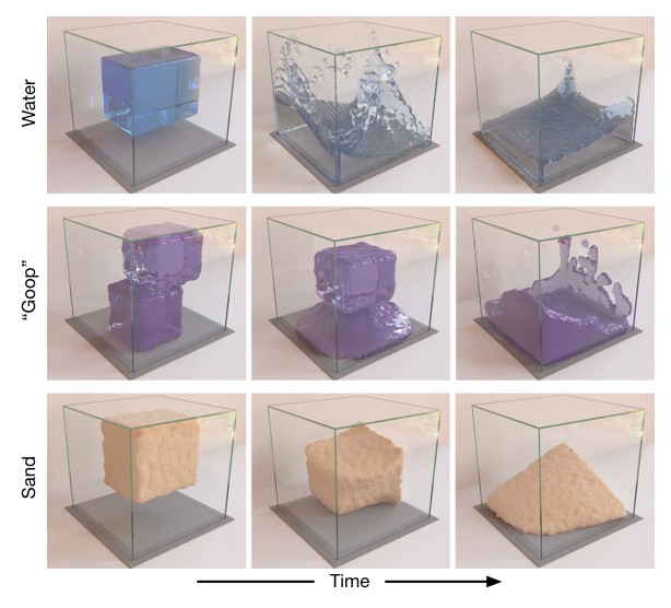
Figure 1. Rollouts of our GNS model for our WATER-3D, GOOP-3D and SAND-3D datasets. It learns to simulate rich materials at resolutions sufficient for high-quality rendering [video].
图 1:我们的 GNS 模型在 WATER-3D、GOOP-3D 和 SAND-3D 数据集上的 rollout。它能在足以做高质量渲染的分辨率上,学习仿真丰富的材料。[视频]
- Introduction
- 引言
Realistic simulators of complex physics are invaluable to many scientific and engineering disciplines, however traditional simulators can be very expensive to create and use. Building a simulator can entail years of engineering effort, and often must trade off generality for accuracy in a narrow range of settings. High-quality simulators require substantial computational resources, which makes scaling up prohibitive. Even the best are often inaccurate due to insufficient knowledge of, or difficulty in approximating, the underlying physics and parameters. An attractive alternative to traditional simulators is to use machine learning to train simulators directly from observed data, however the large state spaces and complex dynamics have been difficult for standard end-to-end learning approaches to overcome.
复杂物理的逼真仿真器,对许多科学与工程学科都极为重要,但传统仿真器的制作和使用往往非常昂贵。做一个仿真器可能要投入多年工程,而且还常常必须牺牲通用性,才能在较窄的设定里换取精度。高质量仿真器需要大量计算资源,规模再往上走就会难以承受。即便是最好的仿真器,也常常因为对底层物理和参数了解不够、或难以近似,而并不准确。相对传统仿真器,一条吸引人的替代路线是用机器学习直接从观测数据训练仿真器;不过状态空间很大、动力学又复杂,一般的端到端学习方法一直不容易对付。
Here we present a powerful machine learning framework for learning to simulate complex systems from data—“Graph Network-based Simulators” (GNS). Our framework imposes strong inductive biases, where rich physical states are represented by graphs of interacting particles, and complex dynamics are approximated by learned message-passing among nodes.
我们在此提出一个从数据中学习仿真复杂系统的有力机器学习框架——“基于图网络的仿真器”(GNS)。该框架施加了很强的归纳偏置:丰富的物理状态由相互作用的粒子图来表示,复杂动力学则由节点之间学习到的消息传递来近似。
We implemented our GNS framework in a single deep learning architecture, and found it could learn to accurately simulate a wide range of physical systems in which fluids, rigid solids, and deformable materials interact with one another. Our model also generalized well to much larger systems and longer time scales than those on which it was trained. While previous learning simulation approaches (Li et al., 2018; Ummenhofer et al., 2020) have been highly specialized for particular tasks, we found our single GNS model performed well across dozens of experiments and was generally robust to hyperparameter choices. Our analyses showed that performance was determined by a handful of key factors: its ability to compute long-range interactions, inductive biases for spatial invariance, and training procedures which mitigate the accumulation of error over long simulated trajectories.
我们用单一的深度学习架构实现了 GNS 框架,并发现它能够学习准确仿真范围广泛的物理系统,其中流体、刚性固体和可变形材料会相互作用。模型还能很好地推广到比训练时更大的系统和更长的时间尺度。以往的可学习仿真方法(Li et al., 2018; Ummenhofer et al., 2020)往往针对特定任务高度特化;我们发现,同一套 GNS 模型在数十项实验中都表现良好,并且总体上对超参数选择比较稳健。分析表明,表现主要由少数几个关键因素决定:计算长程相互作用的能力、关于空间不变性的归纳偏置,以及减轻长仿真轨迹上误差累积的训练程序。
- Related Work
- 相关工作
Our approach focuses on particle-based simulation, which is used widely across science and engineering, e.g., computational fluid dynamics, computer graphics. States are represented as a set of particles, which encode mass, material, movement, etc. within local regions of space. Dynamics are computed on the basis of particles’ interactions within their local neighborhoods. One popular particle-based method for simulating fluids is “smoothed particle hydrodynamics” (SPH) (Monaghan, 1992), which evaluates pressure and viscosity forces around each particle, and updates particles’ velocities and positions accordingly. Other techniques, such as “position-based dynamics” (PBD) (Müller et al., 2007) and “material point method” (MPM) (Sulsky et al., 1995), are more suitable for interacting, deformable materials. In PBD, incompressibility and collision dynamics involve resolving pairwise distance constraints between particles, and directly predicting their position changes. Several differentiable particle-based simulators have recently appeared, e.g., DiffTaichi (Hu et al., 2019), PhiFlow (Holl et al., 2020), and Jax-MD (Schoenholz & Cubuk, 2019), which can backpropagate gradients through the architecture.
我们的方法聚焦于基于粒子的仿真,这类方法在科学和工程中使用很广,例如计算流体力学和计算机图形学。状态被表示为一组粒子,它们在空间的局部区域内编码质量、材料、运动等信息。动力学则根据粒子在其局部邻域内的相互作用来计算。一种流行的流体粒子仿真方法是“光滑粒子流体动力学”(SPH)(Monaghan, 1992),它在每个粒子周围计算压力和黏性力,并据此更新粒子的速度和位置。其他技术,如“基于位置的动力学”(PBD)(Müller et al., 2007)和“物质点法”(MPM)(Sulsky et al., 1995),更适合相互作用的可变形材料。在 PBD 中,不可压缩性和碰撞动力学涉及求解粒子之间的成对距离约束,并直接预测位置变化。近来还出现了若干可微的粒子仿真器,例如 DiffTaichi(Hu et al., 2019)、PhiFlow(Holl et al., 2020)和 Jax-MD(Schoenholz & Cubuk, 2019),它们能够把梯度反向传播过整个架构。
Learning simulations from data (Grzeszczuk et al., 1998) has been an important area of study with applications in physics and graphics. Compared to engineered simulators, a learned simulator can be far more efficient for predicting complex phenomena (He et al., 2019); e.g., (Ladický et al., 2015; Wiewel et al., 2019) learn parts of a fluid simulator for faster prediction.
从数据中学习仿真(Grzeszczuk et al., 1998)一直是一个重要的研究方向,在物理和图形学中都有应用。与手工设计的仿真器相比,学习到的仿真器在预测复杂现象时可以高效得多(He et al., 2019);例如,(Ladický et al., 2015; Wiewel et al., 2019)学习流体仿真器的部分模块,以加快预测。
Graph Networks (GN) (Battaglia et al., 2018)—a type of graph neural network (Scarselli et al., 2008)—have recently proven effective at learning forward dynamics in various settings that involve interactions between many entities. A GN maps an input graph to an output graph with the same structure but potentially different node, edge, and graph-level attributes, and can be trained to learn a form of message-passing (Gilmer et al., 2017), where latent information is propagated between nodes via the edges. GNs and their variants, e.g., “interaction networks”, can learn to simulate rigid body, mass-spring, n-body, and robotic control systems (Battaglia et al., 2016; Chang et al., 2016; Sanchez-Gonzalez et al., 2018; Mrowca et al., 2018; Li et al., 2019; Sanchez-Gonzalez et al., 2019), as well as non-physical systems, such as multi-agent dynamics (Tacchetti et al., 2018; Sun et al., 2019), algorithm execution (Veličković et al., 2020), and other dynamic graph settings (Trivedi et al., 2019; 2017; Yan et al., 2018; Manessi et al., 2020).
图网络(GN)(Battaglia et al., 2018)是一类图神经网络(Scarselli et al., 2008),近来已证明能够在多种涉及大量实体相互作用的设定中学习前向动力学。GN 把输入图映射为结构相同、但节点、边和图级属性可能不同的输出图,并且可以训练成一种消息传递(Gilmer et al., 2017),让隐信息经由边在节点之间传播。GN 及其变体,例如“相互作用网络”,能够学习仿真刚体、质点-弹簧、n 体和机器人控制系统(Battaglia et al., 2016; Chang et al., 2016; Sanchez-Gonzalez et al., 2018; Mrowca et al., 2018; Li et al., 2019; Sanchez-Gonzalez et al., 2019),也能用于非物理系统,例如多智能体动力学(Tacchetti et al., 2018; Sun et al., 2019)、算法执行(Veličković et al., 2020),以及其他动态图设定(Trivedi et al., 2019; 2017; Yan et al., 2018; Manessi et al., 2020)。
Our GNS framework builds on and generalizes several lines of work, especially Sanchez-Gonzalez et al. (2018)’s GN-based model which was applied to various robotic control systems, Li et al. (2018)’s DPI which was applied to fluid dynamics, and Ummenhofer et al. (2020)’s Continuous Convolution (CConv) which was presented as a non-graph-based method for simulating fluids. Crucially, our GNS framework is a general approach to learning simulation, is simpler to implement, and is more accurate across fluid, rigid, and deformable material systems.
我们的 GNS 框架建立在若干工作路线之上,并对其做了推广,尤其是 Sanchez-Gonzalez et al. (2018) 应用于多种机器人控制系统的基于 GN 的模型、Li et al. (2018) 应用于流体动力学的 DPI,以及 Ummenhofer et al. (2020) 作为非基于图的方法提出的连续卷积(CConv)。关键在于,GNS 是一条学习仿真的通用路径,实现更简单,并且在流体、刚体和可变形材料系统上都更准确。
- GNS Model Framework
- GNS 模型框架
3.1. General Learnable Simulation
3.1. 一般的可学习仿真
We assume is the state of the world at time . Applying physical dynamics over timesteps yields a trajectory of states, . A simulator, , models the dynamics by mapping preceding states to causally consequent future states. We denote a simulated “rollout” trajectory as , which is computed iteratively by for each timestep. Simulators compute dynamics information that reflects how the current state is changing, and use it to update the current state to a predicted future state (see Figure 2(a)). An example is a numerical differential equation solver: the equations compute dynamics information, i.e., time derivatives, and the integrator is the update mechanism.
我们假设 是世界在时刻 的状态。把物理动力学作用 个时间步,就得到一条状态轨迹 。仿真器 通过把先前状态映射到具有因果后续关系的未来状态,来建模动力学。我们把一条仿真“rollout”轨迹记为 ,它在每个时间步按 迭代计算。仿真器会计算反映当前状态如何变化的动力学信息,并用它把当前状态更新为预测的未来状态(见图 2(a))。一个例子是数值微分方程求解器:方程计算动力学信息,即时间导数,积分器则是更新机制。
A learnable simulator, , computes the dynamics information with a parameterized function approximator, , whose parameters, , can be optimized for some training objective. The represents the dynamics information, whose semantics are determined by the update mechanism. The update mechanism can be seen as a function which takes the , and uses to predict the next state, . Here we assume a simple update mechanism—an Euler integrator—and that represents accelerations. However, more sophisticated update procedures which call more than once can also be used, such as higher-order integrators (e.g., Sanchez-Gonzalez et al. (2019)).
可学习仿真器 用一个参数化的函数逼近器 来计算动力学信息,其参数 可以按某种训练目标优化。 表示动力学信息,其语义由更新机制决定。更新机制可以看成一个函数:它接收 ,并用 预测下一状态,。这里我们采用一种简单的更新机制——欧拉积分器,并让 表示加速度。不过,也可以使用更复杂、会多次调用 的更新程序,例如高阶积分器(如 Sanchez-Gonzalez et al. (2019))。
3.2. Simulation as Message-Passing on a Graph
3.2. 把仿真看成图上的消息传递
Our learnable simulation approach adopts a particle-based representation of the physical system (see Section 2), i.e., , where each of the particles’ represents its state. Physical dynamics are approximated by interactions among the particles, e.g., exchanging energy and momentum among their neighbors. The way particle-particle interactions are modeled determines the quality and generality of a simulation method—i.e., the types of effects and materials it can simulate, in which scenarios the method performs well or poorly, etc. We are interested in learning these interactions, which should, in principle, allow learning the dynamics of any system that can be expressed as particle dynamics. So it is crucial that different values allow to span a wide range of particle-particle interaction functions.
我们的可学习仿真方法采用基于粒子的物理系统表示(见第 2 节),即 ,其中 个粒子各自的 表示其状态。物理动力学由粒子之间的相互作用来近似,例如在邻域之间交换能量和动量。粒子-粒子相互作用的建模方式,决定了一种仿真方法的质量和通用性——也就是它能仿真哪些效应和材料、在哪些场景下表现好或差,等等。我们关心的是学习这些相互作用;原则上,这应能让我们学习任何可以写成粒子动力学的系统。因此,不同的 值必须让 能够覆盖范围广泛的粒子-粒子相互作用函数,这一点至关重要。
Particle-based simulation can be viewed as message-passing on a graph. The nodes correspond to particles, and the edges correspond to pairwise relations among particles, over which interactions are computed. We can understand methods like SPH in this framework—the messages passed between nodes could correspond to, e.g., evaluating pressure using the density kernel.
基于粒子的仿真可以看成图上的消息传递。节点对应粒子,边对应粒子之间的成对关系,相互作用就在这些边上计算。像 SPH 这样的方法也可以放在这一框架里理解——节点之间传递的消息,可以对应于例如用密度核来计算压力。
We capitalize on the correspondence between particle-based simulators and message-passing on graphs to define a general-purpose based on GNs. Our has three steps—ENCODER, PROCESSOR, DECODER (Battaglia et al., 2018) (see Figure 2(b)).
我们利用粒子仿真器与图上消息传递之间的对应关系,定义一个基于 GN 的通用 。我们的 分为三步:编码器(ENCODER)、处理器(PROCESSOR)、解码器(DECODER)(Battaglia et al., 2018)(见图 2(b))。
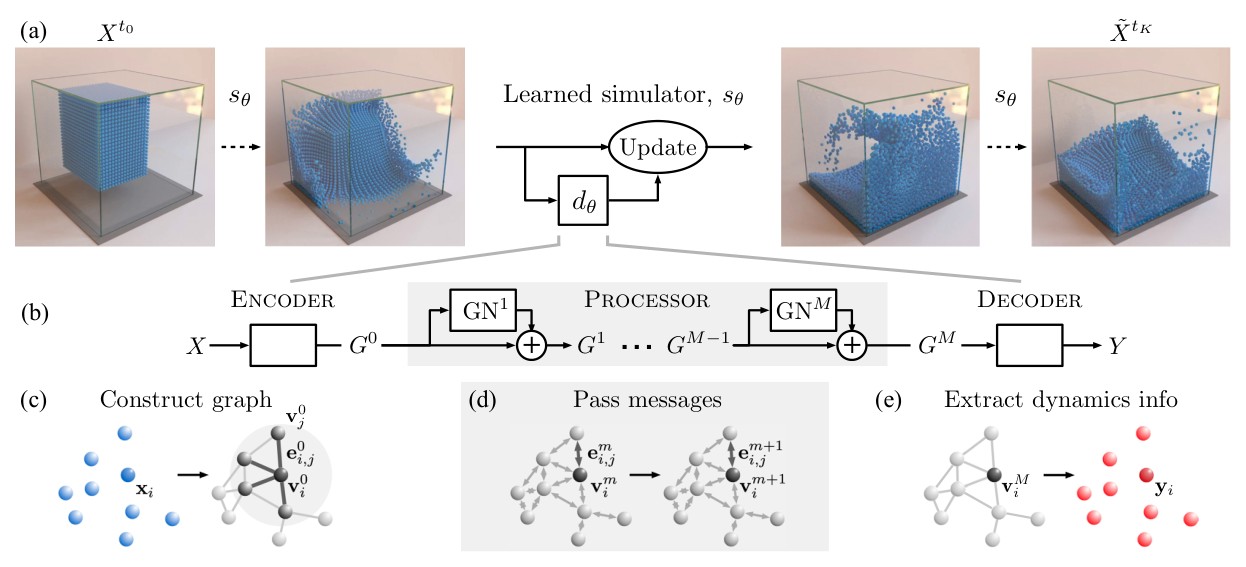
Figure 2. (a) Our GNS predicts future states represented as particles using its learned dynamics model, , and a fixed update procedure. (b) The uses an “encode-process-decode” scheme, which computes dynamics information, , from input state, . (c) The ENCODER constructs latent graph, , from the input state, . (d) The PROCESSOR performs rounds of learned message-passing over the latent graphs, . (e) The DECODER extracts dynamics information, , from the final latent graph, .
图 2。(a) 我们的 GNS 用学习到的动力学模型 和固定的更新程序,预测用粒子表示的未来状态。(b) 采用“编码—处理—解码”方案,从输入状态 计算动力学信息 。(c) 编码器从输入状态 构造隐图 。(d) 处理器在隐图 上执行 轮学习到的消息传递。(e) 解码器从最终隐图 中提取动力学信息 。
ENCODER definition. The embeds the particle-based state representation, , as a latent graph, , where , , and (see Figure 2(b,c)). The node embeddings, , are learned functions of the particles’ states. Directed edges are added to create paths between particle nodes which have some potential interaction. The edge embeddings, , are learned functions of the pairwise properties of the corresponding particles, , e.g., displacement between their positions, spring constant, etc. The graph-level embedding, , can represent global properties such as gravity and magnetic fields (though in our implementation we simply appended those as input node features—see Section 4.2 below).
编码器的定义。 把基于粒子的状态表示 嵌入为隐图 ,其中 ,,(见图 2(b,c))。节点嵌入 是粒子状态的学习函数。对可能发生相互作用的粒子节点,添加有向边以形成路径。边嵌入 是对应粒子成对属性 的学习函数,例如位置之间的位移、弹簧常数等。图级嵌入 可以表示重力、磁场等全局属性(不过在我们的实现里,只是把它们附加为输入节点特征——见下文第 4.2 节)。
PROCESSOR definition. The computes interactions among nodes via steps of learned message-passing, to generate a sequence of updated latent graphs, , where (see Figure 2(b,d)). It returns the final graph, . Message-passing allows information to propagate and constraints to be respected: the number of message-passing steps required will likely scale with the complexity of the interactions.
处理器的定义。 通过 步学习到的消息传递来计算节点之间的相互作用,生成一列更新后的隐图 ,其中 (见图 2(b,d))。它返回最终的图 。消息传递使信息得以传播、约束得以被遵守:所需的消息传递步数,很可能随相互作用的复杂程度而增加。
DECODER definition. The extracts dynamics information from the nodes of the final latent graph, (see Figure 2(b,e)). Learning should cause the representations to reflect relevant dynamics information, such as acceleration, in order to be semantically meaningful to the update procedure.
解码器的定义。 从最终隐图的节点中提取动力学信息,(见图 2(b,e))。学习 应使 表示反映出相关的动力学信息,例如加速度,以便对更新程序具有语义上的意义。
- Experimental Methods
- 实验方法
Code and data available at github.com/deepmind/deepmind-research/tree/master/learning_to_simulate.
代码和数据见 github.com/deepmind/deepmind-research/tree/master/learning_to_simulate。
4.1. Physical Domains
4.1. 物理域
We explored how our GNS learns to simulate in datasets which contained three diverse, complex physical materials: water as a barely damped fluid, chaotic in nature; sand as a granular material with complex frictional behavior; and “goop” as a viscous, plastically deformable material. These materials have very different behavior, and in most simulators, require implementing separate material models or even entirely different simulation algorithms.
我们在包含三种多样而复杂的物理材料的数据集上,考察 GNS 如何学习仿真:水作为一种几乎无阻尼、本质混沌的流体;沙子作为具有复杂摩擦行为的颗粒材料;以及“goop”作为一种黏性、可塑性变形的材料。这些材料的行为差异很大,在大多数仿真器中需要实现各自的材料模型,甚至完全不同的仿真算法。
For one domain, we use Li et al. (2018)’s BOXBATH, which simulates a container of water and a cube floating inside, all represented as particles, using the PBD engine FleX (Macklin et al., 2014).
其中一个域,我们使用 Li et al. (2018) 的 BOXBATH:它用 PBD 引擎 FleX(Macklin et al., 2014)仿真一容器水和其中漂浮的立方体,全部用粒子表示。
We also created WATER-3D, a high-resolution 3D water scenario with randomized water position, initial velocity and volume, comparable to Ummenhofer et al. (2020)’s containers of water. We used SPlisHSPlasH (Bender & Koschier, 2015), a SPH-based fluid simulator with strict volume preservation to generate this dataset.
我们还创建了 WATER-3D,这是一个高分辨率的三维水场景,水的位置、初速度和体积都经过随机化,可与 Ummenhofer et al. (2020) 的容器水场景相比较。该数据集用 SPlisHSPlasH(Bender & Koschier, 2015)生成,这是一个严格保持体积的、基于 SPH 的流体仿真器。
For most of our domains, we use the Taichi-MPM engine (Hu et al., 2018) to simulate a variety of challenging 2D and 3D scenarios. We chose MPM for the simulator because it can simulate a very wide range of materials, and also has some different properties than PBD and SPH, e.g., particles may become compressed over time.
对大多数域,我们使用 Taichi-MPM 引擎(Hu et al., 2018)来仿真多种有挑战性的二维和三维场景。选择 MPM 做仿真器,是因为它能仿真非常广泛的材料,并且与 PBD 和 SPH 还有一些不同性质,例如粒子可能随时间被压缩。
Our datasets typically contained 1000 train, 100 validation and 100 test trajectories, each simulated for 300-2000 timesteps (tailored to the average duration for the various materials to come to a stable equilibrium). A detailed listing of all our datasets can be found in the Supplementary Materials B.
我们的数据集通常包含 1000 条训练轨迹、100 条验证轨迹和 100 条测试轨迹,每条仿真 300–2000 个时间步(按各种材料到达稳定平衡的平均时长来设定)。全部数据集的详细列表见 Supplementary Materials B。
4.2. GNS Implementation Details
4.2. GNS 实现细节
We implemented the components of the GNS framework using standard deep learning building blocks, and used standard nearest neighbor algorithms (Dong et al., 2011; Chen et al., 2009; Tang et al., 2016) to construct the graph.
我们用标准的深度学习构件实现 GNS 框架中的各部件,并用标准的最近邻算法(Dong et al., 2011; Chen et al., 2009; Tang et al., 2016)来构图。
Input and output representations. Each particle’s input state vector represents position, a sequence of previous velocities, and features that capture static material properties (e.g., water, sand, goop, rigid, boundary particle), , respectively. The global properties of the system, , include external forces and global material properties, when applicable. The prediction targets for supervised learning are the per-particle average acceleration, . Note that in our datasets, we only require vectors: the and are computed from using finite differences. For full details of these input and target features, see Supplementary Material Section B.
输入与输出表示。每个粒子的输入状态向量表示位置、一段 的既往速度,以及刻画静态材料属性的特征(例如水、沙、goop、刚性、边界粒子),即 。系统的全局属性 在适用时包括外力和全局材料属性。监督学习的预测目标是每个粒子的平均加速度 。注意,在我们的数据集中只需要 向量: 和 由 通过有限差分计算得到。这些输入和目标特征的完整细节见 Supplementary Material 第 B 节。
is a hyperparameter which we explore in our experiments.
是一个超参数,我们在实验中做了考察。
ENCODER details. The ENCODER constructs the graph structure by assigning a node to each particle and adding edges between particles within a “connectivity radius”, , which reflected local interactions of particles, and which was kept constant for all simulations of the same resolution. For generating rollouts, on each timestep the graph’s edges were recomputed by a nearest neighbor algorithm, to reflect the current particle positions.
编码器细节。编码器为每个粒子分配一个节点,并在“连通半径” 内的粒子之间加边,从而构造图结构 。 反映粒子的局部相互作用,并且在同一分辨率的全部仿真中保持不变。生成 rollout 时,每个时间步都用最近邻算法重新计算图的边,以反映当前的粒子位置。
The ENCODER implements and as multilayer perceptrons (MLP), which encode node features and edge features into the latent vectors, and , of size 128.
编码器把 和 实现为多层感知机(MLP),分别把节点特征和边特征编码为大小为 128 的隐向量 和 。
We tested two ENCODER variants, distinguished by whether they use absolute versus relative positional information. For the absolute variant, the input to was the described above, with the globals features concatenated to it. The input to , i.e., , did not actually carry any information and was discarded, with the in set to a trainable fixed bias vector. The relative ENCODER variant was designed to impose an inductive bias of invariance to absolute spatial location. The was forced to ignore information within by masking it out. The was provided with the relative positional displacement, and its magnitude, . Both variants concatenated the global properties onto each before passing it to .
我们测试了两种编码器变体,区别在于使用绝对位置信息还是相对位置信息。对绝对变体, 的输入就是上面描述的 ,并拼接上全局特征。 的输入 实际上不携带信息,因而被丢弃, 中的 被设为一个可训练的固定偏置向量。相对编码器变体旨在施加对绝对空间位置不变的归纳偏置。通过掩码, 被强制忽略 中的 信息。 则被提供相对位置位移及其模长,。两种变体都把全局属性 拼到每个 上,再送入 。
Similarly, relative velocities could be used to enforce invariance to inertial frames of reference.
类似地,也可以使用相对速度,以施加对惯性参考系的不变性。
PROCESSOR details. Our processor uses a stack of GNs (where is a hyperparameter) with identical structure, MLPs as internal edge and node update functions, and either shared or unshared parameters (as analyzed in Results Section 5.4). We use GNs without global features or global updates (similar to an interaction network), and with a residual connections between the input and output latent node and edge attributes.
处理器细节。我们的处理器使用一叠 个结构相同的 GN( 为超参数),内部的边和节点更新函数为 MLP,参数可以共享或不共享(见结果第 5.4 节的分析)。我们使用不含全局特征或全局更新的 GN(类似于相互作用网络),并在输入与输出的隐节点、隐边属性之间加入残差连接。
In preliminary experiments we also attempted using a PROCESSOR with a full GN and a global latent state, for which the global features are encoded with a separate MLP.
在初步实验中,我们也曾尝试过使用带完整 GN 和全局隐状态的处理器,此时全局特征 用单独的 MLP 来编码。
DECODER details. Our decoder’s learned function, , is an MLP. After the DECODER, the future position and velocity are updated using an Euler integrator, so the corresponds to accelerations, , with 2D or 3D dimension, depending on the physical domain. As mentioned above, the supervised training outputs were simply these, vectors.
解码器细节。解码器的学习函数 是一个 MLP。解码器之后,用欧拉积分器更新未来的位置和速度,因此 对应于加速度 ,维数为二维或三维,取决于物理域。如上所述,监督训练的输出就是这些 向量。
Note that in this case optimizing for acceleration is equivalent to optimizing for position, because the acceleration is computed as first order finite difference from the position and we use an Euler integrator to update the position.
注意,在这种情况下优化加速度等价于优化位置,因为加速度是由位置的一阶有限差分计算得到的,并且我们用欧拉积分器来更新位置。
Neural network parameterizations. All MLPs have two hidden layers (with ReLU activations), followed by a non-activated output layer, each layer with size of 128. All MLPs (except the output decoder) are followed by a LayerNorm (Ba et al., 2016) layer, which we generally found improved training stability.
神经网络参数化。所有 MLP 都有两个隐层(使用 ReLU 激活),再加上一个无激活的输出层,每层大小均为 128。除输出解码器外,所有 MLP 后面都接一层 LayerNorm(Ba et al., 2016),我们总体上发现这能改善训练稳定性。
4.3. Training
4.3. 训练
Software. We implemented our models using TensorFlow 1, Sonnet 1, and the “Graph Nets” library (2018).
软件。我们使用 TensorFlow 1、Sonnet 1 以及 “Graph Nets” 库(2018)实现模型。
Training noise. Modeling a complex and chaotic simulation system requires the model to mitigate error accumulation over long rollouts. Because we train our models on ground-truth one-step data, they are never presented with input data corrupted by this sort of accumulated noise. This means that when we generate a rollout by feeding the model with its own noisy, previous predictions as input, the fact that its inputs are outside the training distribution may lead it to make more substantial errors, and thus rapidly accumulate further error. We use a simple approach to make the model more robust to noisy inputs: at training we corrupt the input velocities of the model with random-walk noise (adjusting input positions), so the training distribution is closer to the distribution generated during rollouts. See Supplementary Materials B for full details.
训练噪声。要对复杂而混沌的仿真系统建模,模型必须减轻长 rollout 上的误差累积。因为我们在真值的单步数据上训练,模型从未见过被这类累积噪声污染的输入。这意味着,当我们把模型自己带噪声的先前预测再喂回去生成 rollout 时,输入已落在训练分布之外,可能使它犯下更严重的错误,从而迅速积累更多误差。我们用一种简单办法提高模型对噪声输入的稳健性:训练时用随机游走噪声 污染模型的输入速度(并相应调整输入位置),使训练分布更接近 rollout 时产生的分布。完整细节见 Supplementary Materials B。
Normalization. We normalize all input and target vectors elementwise to zero mean and unit variance, using statistics computed online during training. Preliminary experiments showed that normalization led to faster training, though converged performance was not noticeably improved.
归一化。我们把全部输入和目标向量按元素归一化到零均值、单位方差,统计量在训练过程中在线计算。初步实验表明,归一化能加快训练,不过收敛后的表现没有明显提高。
Loss function and optimization procedures. We randomly sampled particle state pairs from training trajectories, calculated target accelerations (subtracting the noise added to the most recent input velocity), and computed the loss on the predicted per-particle accelerations, i.e., . We optimized the model parameters over this loss with the Adam optimizer (Kingma & Ba, 2014), using a nominal mini-batch size of 2. We performed a maximum of 20M gradient update steps, with exponential learning rate decay from to . While models can train in significantly less steps, we avoid aggressive learning rates to reduce variance across datasets and make comparisons across settings more fair.
损失函数与优化程序。我们从训练轨迹中随机采样粒子状态对 ,计算目标加速度 (减去加在最近一次输入速度上的噪声),并对预测的逐粒子加速度计算 损失,即 。我们用 Adam 优化器(Kingma & Ba, 2014)按该损失优化模型参数 ,标称小批量大小为 2。最多进行 2000 万次梯度更新,学习率从 指数衰减到 。虽然模型可以用少得多的步数训练完,但我们避免过于激进的学习率,以减小跨数据集的方差,并使不同设定之间的比较更公平。
The actual batch size varies at each step dynamically. See Supplementary Material for more details.
实际的批量大小在每一步会动态变化。更多细节见 Supplementary Material。
We evaluated our models regularly during training by producing full-length rollouts on 5 held-out validation trajectories, and recorded the associated model parameters for best rollout MSE. We stopped training when we observed negligible decrease in MSE, which, on GPU/TPU hardware, was typically within a few hours for smaller, simpler datasets, and up to a week for the larger, more complex datasets.
训练过程中,我们定期在 5 条留出的验证轨迹上生成全长 rollout 来评估模型,并记录 rollout 均方误差最好时对应的模型参数。当观察到均方误差几乎不再下降时停止训练;在 GPU/TPU 硬件上,较小、较简单的数据集通常只需几小时,较大、较复杂的数据集则最多需要一周。
Table 1. List of maximum number of particles , sequence length , and quantitative model accuracy (MSE) on the held-out test set. All domain names are also hyperlinks to the video website.
| Experimental domain | 1-step () | Rollout () | ||
|---|---|---|---|---|
| WATER-3D (SPH) | 13k | 800 | 8.66 | 10.1 |
| SAND-3D | 20k | 350 | 1.42 | 0.554 |
| GOOP-3D | 14k | 300 | 1.32 | 0.618 |
| WATER-3D-S (SPH) | 5.8k | 800 | 9.66 | 9.52 |
| BOXBATH (PBD) | 1k | 150 | 54.5 | 4.2 |
| WATER | 1.9k | 1000 | 2.82 | 17.4 |
| SAND | 2k | 320 | 6.23 | 2.37 |
| GOOP | 1.9k | 400 | 2.91 | 1.89 |
| MULTIMATERIAL | 2k | 1000 | 1.81 | 16.9 |
| FLUIDSHAKE | 1.3k | 2000 | 2.1 | 20.1 |
| WATERDROP | 1k | 1000 | 1.52 | 7.01 |
| WATERDROP-XL | 7.1k | 1000 | 1.23 | 14.9 |
| WATERRAMPS | 2.3k | 600 | 4.91 | 11.6 |
| SANDRAMPS | 3.3k | 400 | 2.77 | 2.07 |
| RANDOMFLOOR | 3.4k | 600 | 2.77 | 6.72 |
| CONTINUOUS | 4.3k | 400 | 2.06 | 1.06 |
表 1。各实验域的最大粒子数 、序列长度 ,以及在留出测试集上的定量模型精度(MSE)。所有域名同时也是指向视频网站的超链接。
| 实验域 | 单步 () | Rollout () | ||
|---|---|---|---|---|
| WATER-3D (SPH) | 13k | 800 | 8.66 | 10.1 |
| SAND-3D | 20k | 350 | 1.42 | 0.554 |
| GOOP-3D | 14k | 300 | 1.32 | 0.618 |
| WATER-3D-S (SPH) | 5.8k | 800 | 9.66 | 9.52 |
| BOXBATH (PBD) | 1k | 150 | 54.5 | 4.2 |
| WATER | 1.9k | 1000 | 2.82 | 17.4 |
| SAND | 2k | 320 | 6.23 | 2.37 |
| GOOP | 1.9k | 400 | 2.91 | 1.89 |
| MULTIMATERIAL | 2k | 1000 | 1.81 | 16.9 |
| FLUIDSHAKE | 1.3k | 2000 | 2.1 | 20.1 |
| WATERDROP | 1k | 1000 | 1.52 | 7.01 |
| WATERDROP-XL | 7.1k | 1000 | 1.23 | 14.9 |
| WATERRAMPS | 2.3k | 600 | 4.91 | 11.6 |
| SANDRAMPS | 3.3k | 400 | 2.77 | 2.07 |
| RANDOMFLOOR | 3.4k | 600 | 2.77 | 6.72 |
| CONTINUOUS | 4.3k | 400 | 2.06 | 1.06 |
4.4. Evaluation
4.4. 评测
To report quantitative results, we evaluated our models after training converged by computing one-step and rollout metrics on held-out test trajectories, drawn from the same distribution of initial conditions used for training. We used particle-wise MSE as our main metric between ground truth and predicted data, both for rollout and one-step predictions, averaging across time, particle and spatial axes. We also investigated distributional metrics including optimal transport (OT) (Villani, 2003) (approximated by the Sinkhorn Algorithm (Cuturi, 2013)), and Maximum Mean Discrepancy (MMD) (Gretton et al., 2012). For the generalization experiments we also evaluate our models on a number of initial conditions drawn from distributions different than those seen during training, including, different number of particles, different object shapes, different number of objects, different initial positions and velocities and longer trajectories. See Supplementary Materials B for full details on metrics and evaluation.
为报告定量结果,我们在训练收敛后,于留出的测试轨迹上计算单步指标和 rollout 指标;这些轨迹的初始条件与训练时来自同一分布。我们以逐粒子均方误差作为主要指标,比较真值与预测数据,对 rollout 和单步预测都适用,并在时间、粒子和空间轴上取平均。我们还考察了分布型指标,包括最优传输(OT)(Villani, 2003)(用 Sinkhorn 算法近似(Cuturi, 2013))以及最大均值差异(MMD)(Gretton et al., 2012)。在泛化实验中,我们还在与训练时不同分布抽出的若干初始条件上评估模型,包括不同的粒子数、不同的物体形状、不同的物体数量、不同的初始位置与速度,以及更长的轨迹。指标与评测的完整细节见 Supplementary Materials B。
- Results
- 结果
Our main findings are that our GNS model can learn accurate, high-resolution, long-term simulations of different fluids, deformables, and rigid solids, and it can generalize well beyond training to much longer, larger, and challenging settings. In Section 5.5 below, we compare our GNS model to two recent, related approaches, and find our approach was simpler, more generally applicable, and more accurate.
我们的主要发现是:GNS 模型能够学习对不同流体、可变形体和刚性固体做准确、高分辨率、长时间的仿真,并且能够很好地推广到比训练时更长、更大、更具挑战性的设定。在下面第 5.5 节中,我们把 GNS 与两种近期相关方法做了比较,发现我们的方法更简单、更通用,也更准确。
To challenge the robustness of our architecture, we used a single set of model hyperparameters for training across all of our experiments. Our GNS architecture used the relative ENCODER variant, 10 steps of message-passing, with unshared GN parameters in the PROCESSOR. We applied noise with a scale of to the input states during training.
为检验架构的稳健性,我们在全部实验中都用同一组模型超参数来训练。GNS 架构采用相对编码器变体、10 步消息传递,并且处理器中的 GN 参数不共享。训练时对输入状态施加尺度为 的噪声。
5.1. Simulating Complex Materials
5.1. 仿真复杂材料
Our GNS model was very effective at learning to simulate different complex materials. Table 1 shows the one-step and rollout accuracy, as MSE, for all experiments. For intuition about what these numbers mean, the edge length of the container was approximately 1.0, and Figure 3(a-c) shows rendered images of the rollouts of our model, compared to ground truth. Visually, the model’s rollouts are quite plausible. Though specific model-generated trajectories can be distinguished from ground truth when compared side-by-side, it is difficult to visually classify individual videos as generated from our model versus the ground truth simulator.
GNS 模型在学习仿真不同的复杂材料上非常有效。表 1 给出了全部实验的单步和 rollout 精度(以 MSE 计)。为了直观理解这些数字的含义,容器的边长大约为 1.0;图 3(a-c) 给出了模型 rollout 与真值的渲染图像。从视觉上看,模型的 rollout 相当合理。虽然把具体的模型生成轨迹与真值并排放在一起时仍能区分,但很难仅凭观感把单个视频判定为来自我们的模型还是来自真值仿真器。
All rollout videos can be found here: https://sites.google.com/view/learning-to-simulate
全部 rollout 视频见:https://sites.google.com/view/learning-to-simulate
Our GNS model scales to large amounts of particles and very long rollouts. With up to 19k particles in our 3D domains—substantially greater than demonstrated in previous methods—GNS can operate at resolutions high enough for practical prediction tasks and high-quality 3D renderings (e.g., Figure 1). And although our models were trained to make one-step predictions, the long-term trajectories remain plausible even over thousands of rollout timesteps.
GNS 模型可以扩展到大量粒子和非常长的 rollout。在我们的三维域中,粒子数最多可达 1.9 万——明显多于以往方法所展示的规模——因而 GNS 能够在足以支撑实际预测任务和高质量三维渲染的分辨率上运行(例如图 1)。而且,尽管模型按单步预测来训练,长期轨迹即使在数千个 rollout 时间步上仍然看起来合理。
The GNS model could also learn how the materials respond to unpredictable external forces. In the FLUIDSHAKE domain, a container filled with water is being moved side-to-side, causing splashes and irregular waves.
GNS 模型还能学习材料如何响应不可预知的外力。在 FLUIDSHAKE 域中,一只装满水的容器被左右移动,从而产生飞溅和不规则的波浪。
Our model could also simulate fluid interacting with complicated static obstacles, as demonstrated by our WATERRAMPS and SANDRAMPS domains in which water or sand pour over 1-5 obstacles. Figure 3(d) depicts comparisons between our model and ground truth, and Table 1 shows quantitative performance measures.
模型也能仿真流体与复杂静态障碍物的相互作用,这体现在 WATERRAMPS 和 SANDRAMPS 域中:水或沙子从 1 到 5 个障碍物上倾泻而下。图 3(d) 给出了模型与真值的比较,表 1 给出了定量性能指标。
We also trained our model on continuously varying material parameters. In the CONTINUOUS domain, we varied the friction angle of a granular material, to yield behavior similar to a liquid (), sand (), or gravel (). Our results and videos show that our model can account for these continuous variations, and even interpolate between them: a model trained with the region held out in training can accurately predict within that range. Additional quantitative results are available in Supplementary Materials C.
我们还在连续变化的材料参数上训练了模型。在 CONTINUOUS 域中,我们改变颗粒材料的摩擦角,使其行为分别接近液体()、沙子()或砾石()。结果和视频表明,模型能够刻画这些连续变化,甚至可以在其间插值:训练时留出 区间的模型,仍能在该范围内做出准确预测。更多定量结果见 Supplementary Materials C。
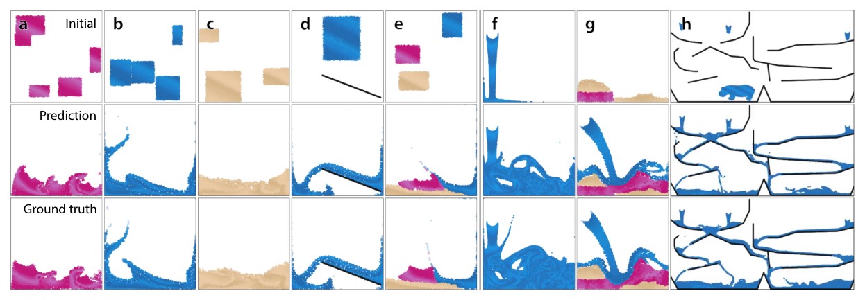
Figure 3. We can simulate many materials, from (a) GOOP over (b) WATER to (c) SAND, and (d) their interaction with rigid obstacles (WATERRAMPS). We can even train a single model on (e) multiple materials and their interaction (MULTIMATERIAL). We applied pre-trained models on several out-of-distribution tasks, involving (f) high-res turbulence (trained on WATERRAMPS), (g) multi-material interactions with unseen objects (trained on MULTIMATERIAL), and (h) generalizing on significantly larger domains (trained on WATERRAMPS). In the two bottom rows, we show a comparison of our model’s prediction with the ground truth on the final frame for goop and sand, and on a representative mid-trajectory frame for water.
图 3。我们可以仿真多种材料,从 (a) GOOP 到 (b) WATER 再到 (c) SAND,以及 (d) 它们与刚性障碍物的相互作用(WATERRAMPS)。我们甚至可以在 (e) 多种材料及其相互作用(MULTIMATERIAL)上训练单一模型。我们把预训练模型用到若干分布外任务上,包括 (f) 高分辨率湍流(在 WATERRAMPS 上训练)、(g) 与未见物体的多材料相互作用(在 MULTIMATERIAL 上训练),以及 (h) 在显著更大的域上泛化(在 WATERRAMPS 上训练)。在下面两行中,我们对 goop 和沙子给出模型预测与真值在最后一帧上的比较,对水则给出轨迹中段一个有代表性的帧。
5.2. Multiple Interacting Materials
5.2. 多种相互作用的材料
So far we have reported results of training identical GNS architectures separately on different systems and materials. However, we found we could go a step further and train a single architecture with a single set of parameters to simulate all of our different materials, interacting with each other in a single system.
到目前为止,我们报告的是把相同的 GNS 架构分别在不同系统和材料上训练的结果。不过我们发现还可以再进一步:用同一套架构、同一组参数,在单一系统中仿真我们全部不同的材料,并让它们相互作用。
In our MULTIMATERIAL domain, the different materials could interact with each other in complex ways, which means the model had to effectively learn the product space of different interactions (e.g., water-water, sand-sand, water-sand, etc.). The behavior of these systems was often much richer than the single-material domains: the stiffer materials, such as sand and goop, could form temporary semi-rigid obstacles, which the water would then flow around. Figure 3(e) and this video shows renderings of such rollouts. Visually, our model’s performance in MULTIMATERIAL is comparable to its performance when trained on those materials individually.
在 MULTIMATERIAL 域中,不同材料能够以复杂方式相互作用,这意味着模型必须有效学习不同相互作用的乘积空间(例如水-水、沙-沙、水-沙等)。这些系统的行为往往比单材料域丰富得多:沙子和 goop 这类更硬的材料可以形成临时的半刚性障碍,水再从旁边流过。图 3(e) 和该视频给出了这类 rollout 的渲染。从视觉上看,模型在 MULTIMATERIAL 上的表现,与在这些材料上单独训练时相当。
5.3. Generalization
5.3. 泛化
We found that the GNS generalizes well even beyond its training distributions, which suggests it learns a more general-purpose understanding of the materials and physical processes experienced during training.
我们发现,GNS 即使在训练分布之外也能很好地泛化,这表明它学到了对训练中所见材料和物理过程更通用的理解。
To examine its capacity for generalization, we trained a GNS architecture on WATERRAMPS, whose initial conditions involved a square region of water in a container, with 1-5 ramps of random orientation and location. After training, we tested the model on several very different settings. In one generalization condition, rather than all water being present in the initial timestep, we created an “inflow” that continuously added water particles to the scene during the rollout, as shown in Figure 3(f). When unrolled for 2500 time steps, the scene contained 28k particles—an order of magnitude more than the 2.5k particles used in training—and the model was able to predict complex, highly chaotic dynamics not experienced during training, as can be seen in this video. The predicted dynamics were visually similar to the ground truth sequence.
为考察其泛化能力,我们在 WATERRAMPS 上训练 GNS:其初始条件是容器中一块方形水域,并带有 1 到 5 个随机朝向和位置的坡道。训练之后,我们在几种非常不同的设定上测试模型。在一种泛化条件里,并不是一开始就放入全部的水,而是设置一个“入流”,在 rollout 过程中持续向场景添加水粒子,如图 3(f) 所示。当展开 2500 个时间步时,场景中有 2.8 万个粒子——比训练时使用的 2500 个粒子多出一个数量级——模型仍能预测训练中未曾见过的、高度混沌的复杂动力学,见该视频。预测的动力学在视觉上与真值序列相近。
Because we used relative displacements between particles as input to our model, in principle the model should handle scenes with much larger spatial extent at test time. We evaluated this on a much larger domain, with several inflows over a complicated arrangement of slides and ramps (see Figure 3(h), video here). The test domain’s spatial width × height were 8.0 × 4.0, which was 32x larger than the training domain’s area; at the end of the rollout, the number of particles was 85k, which was 34x more than during training; we unrolled the model for 5000 steps, which was 8x longer than the training trajectories. We conducted a similar experiment with sand on the SANDRAMPS domain, testing model generalization to hourglass-shaped ramps.
因为我们把粒子之间的相对位移作为模型输入,原则上模型在测试时应能处理空间范围大得多的场景。我们在一个大得多的域上评估了这一点:若干入流经过复杂排布的滑道和坡道(见图 3(h),视频见此)。测试域的空间宽 × 高为 8.0 × 4.0,面积是训练域的 32 倍;rollout 结束时粒子数为 8.5 万,是训练时的 34 倍;我们把模型展开了 5000 步,是训练轨迹长度的 8 倍。我们还在 SANDRAMPS 域上用沙子做了类似实验,测试模型对沙漏形坡道的泛化。
As a final, extreme test of generalization, we applied a model trained on MULTIMATERIAL to a custom test domain with inflows of various materials and shapes (Figure 3(g)). The model learned about frictional behavior between different materials (sand on sticky goop, versus slippery floor), and that the model generalized well to unseen shapes, such as hippo-shaped chunks of goop and water, falling from midair, as can be observed in this video.
作为最后一项极端的泛化测试,我们把在 MULTIMATERIAL 上训练的模型,用到一个带有多种材料和形状入流的定制测试域上(图 3(g))。模型学到了不同材料之间的摩擦行为(沙子在黏性 goop 上,对比滑的地面),并且很好地泛化到未见过的形状,例如从半空落下的河马形状的 goop 和水块,见该视频。
5.4. Key Architectural Choices
5.4. 关键的架构选择
We performed a comprehensive analysis of our GNS’s architectural choices to discover what influenced performance most heavily. We analyzed a number of hyperparameter choices—e.g., number of MLP layers, linear encoder and decoder functions, global latent state in the PROCESSOR—but found these had minimal impact on performance (see Supplementary Materials C for details).
我们对 GNS 的架构选择做了全面分析,以找出对性能影响最大的因素。我们分析了若干超参数选择——例如 MLP 层数、线性的编码器和解码器函数、处理器中的全局隐状态——但发现这些对性能的影响很小(细节见 Supplementary Materials C)。
While our GNS model was generally robust to architectural and hyperparameter settings, we also identified several factors which had more substantial impact:
尽管 GNS 模型总体上对架构和超参数设定比较稳健,我们也找出了几个影响更显著的因素:
- the number of message-passing steps,
- 消息传递的步数,
- shared vs. unshared PROCESSOR GN parameters,
- 处理器中 GN 参数共享与不共享,
- the connectivity radius,
- 连通半径,
- the scale of noise added to the inputs during training,
- 训练时加在输入上的噪声尺度,
- relative vs. absolute ENCODER.
- 相对编码器与绝对编码器。
We varied these choices systematically for each axis, fixing all other axes with the default architecture’s choices, and report their impact on model performance in the GOOP domain (Figure 4).
我们对每个轴系统变化这些选择,其余轴固定为默认架构的设定,并在 GOOP 域上报告它们对模型性能的影响(图 4)。
For (1), Figure 4(a,b) shows that a greater number of message-passing steps yielded improved performance in both one-step and rollout accuracy. This is likely because increasing allows computing longer-range, and more complex, interactions among particles. Because computation time scales linearly with , in practice it is advisable to use the smallest that still provides desired performance.
对 (1),图 4(a,b) 表明,更多的消息传递步数 能同时提高单步和 rollout 精度。这很可能是因为增大 可以计算粒子之间更长程、更复杂的相互作用。由于计算时间随 线性增加,实践中宜采用仍能达到所需性能的最小 。
For (2), Figure 4(c,d) shows that models with unshared GN parameters in the PROCESSOR yield better accuracy, especially for rollouts. Shared parameters imposes a strong inductive bias that makes the PROCESSOR analogous to a recurrent model, while unshared parameters are more analogous to a deep architecture, which incurs times more parameters. In practice, we found marginal difference in computational costs or overfitting, so we conclude that using unshared parameters has little downside.
对 (2),图 4(c,d) 表明,处理器中 GN 参数不共享的模型精度更好,尤其是在 rollout 上。共享参数施加了很强的归纳偏置,使处理器类似于循环模型;不共享参数则更类似于深层架构,参数量会增加 倍。实践中,我们几乎没有发现计算代价或过拟合方面的明显差异,因此认为使用不共享参数几乎没有坏处。
For (3), Figure 4(e,f) shows that greater connectivity values yield lower error. Similar to increasing , larger neighborhoods allow longer-range communication among nodes. Since the number of edges increases with , more computation and memory is required, so in practice the minimal that gives desired performance should be used.
对 (3),图 4(e,f) 表明,更大的连通半径 会带来更低的误差。与增大 类似,更大的邻域允许节点之间进行更长程的通信。由于边数随 增加,需要更多计算和内存,因此实践中应采用仍能达到所需性能的最小 。
For (4), we observed that rollout accuracy is best for an intermediate noise scale (see Figure 4(g,h)), consistent with our motivation for using it (see Section 4.3). We also note that one-step accuracy decreases with increasing noise scale. This is not surprising: adding noise makes the training distribution less similar to the uncorrupted distribution used for one-step evaluation.
对 (4),我们观察到 rollout 精度在中等噪声尺度下最好(见图 4(g,h)),这与我们使用噪声的动机一致(见第 4.3 节)。我们还注意到,单步精度会随噪声尺度增大而下降。这并不奇怪:加入噪声会使训练分布不那么接近用于单步评测的、未被污染的分布。
For (5), Figure 4(i,j) shows that the relative ENCODER is clearly better than the absolute version. This is likely because the underlying physical processes that are being learned are invariant to spatial position, and the relative ENCODER’s inductive bias is consistent with this invariance.
对 (5),图 4(i,j) 表明相对编码器明显优于绝对版本。这很可能是因为所学习的底层物理过程对空间位置是不变的,而相对编码器的归纳偏置与这一不变性相一致。
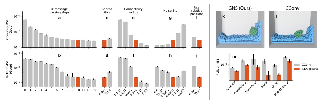
Figure 4. (left) Effect of different ablations (grey) against our model (red) on the one-step error (a,c,e,g,i) and the rollout error (b,d,f,h,j). Bars show the median seed performance averaged across the entire GOOP test dataset. Error bars display lower and higher quartiles, and are shown for the default parameters. (right) Comparison of average performance of our GNS model to CConv. (k,l) Qualitative comparison between GNS (k) and CConv (l) in BOXBATH after 50 rollout steps (video link). (m) Quantitative comparison of our GNS model (red) to the CConv model (grey) across the test set. For our model, we trained one or more seeds using the same set of hyper-parameters and show results for all seeds. For the CConv model we ran several variations including different radius sizes, noise levels, and number of unroll steps during training, and show the result for the best seed. Errors bars show the standard error of the mean across all of the trajectories in the test set (95% confidence level).
图 4。(左)不同消融(灰色)相对我们的模型(红色)对单步误差(a,c,e,g,i)和 rollout 误差(b,d,f,h,j)的影响。柱状图给出在整个 GOOP 测试集上平均后的种子中位数表现。误差棒给出下四分位与上四分位,并在默认参数下标出。(右)我们的 GNS 模型与 CConv 的平均表现比较。(k,l) 在 BOXBATH 上展开 50 步后,GNS (k) 与 CConv (l) 的定性比较(视频链接)。(m) 在测试集上对我们的 GNS 模型(红色)与 CConv 模型(灰色)的定量比较。对我们的模型,我们用同一组超参数训练一个或多个种子,并给出全部种子的结果。对 CConv 模型,我们运行了若干变体,包括不同的半径大小、噪声水平和训练时的展开步数,并给出最佳种子的结果。误差棒给出测试集全部轨迹上均值的标准误差(95% 置信水平)。
5.5. Comparisons to Previous Models
5.5. 与以往模型的比较
We compared our approach to two recent papers which explored learned fluid simulators using particle-based approaches. Li et al. (2018)’s DPI studied four datasets of fluid, deformable, and solid simulations, and presented four different, distinct architectures, which were similar to Sanchez-Gonzalez et al. (2018)’s, with additional features such as hierarchical latent nodes. When training our GNS model on DPI’s BOXBATH domain, we found it could learn to simulate the rigid solid box floating in water, faithfully maintaining the stiff relative displacements among rigid particles, as shown Figure 4(k) and this video. Our GNS model did not require any modification—the box particles’ material type was simply a feature in the input vector—while DPI required a specialized hierarchical mechanism and forced all box particles to preserve their relative displacements with each other. Presumably the relative ENCODER and training noise alleviated the need for such mechanisms.
我们把方法与两篇近期用粒子法探索可学习流体仿真器的论文做了比较。Li et al. (2018) 的 DPI 研究了四个流体、可变形体和固体仿真数据集,并给出了四种不同、互有区别的架构,它们与 Sanchez-Gonzalez et al. (2018) 的工作相似,并增加了层级隐节点等特征。当在 DPI 的 BOXBATH 域上训练 GNS 时,我们发现它能够学习仿真漂浮在水中的刚性盒子,并忠实地保持刚性粒子之间僵硬的相对位移,如图 4(k) 和该视频所示。我们的 GNS 模型不需要任何改动——盒子粒子的材料类型只是输入向量中的一个特征——而 DPI 需要专门的层级机制,并强制所有盒子粒子彼此保持相对位移。相对编码器和训练噪声大概减轻了对这类机制的需要。
Ummenhofer et al. (2020)’s CConv propagates information across particles, and uses particle update functions and training procedures which are carefully tailored to modeling fluid dynamics (e.g., an SPH-like local kernel, different sub-networks for fluid and boundary particles, a loss function that weights slow particles with few neighbors more heavily). Ummenhofer et al. (2020) reported CConv outperformed DPI, so we quantitatively compared our GNS model to CConv. We implemented CConv as described in its paper, plus two additional versions which borrowed our noise and multiple input states, and performed hyperparameter sweeps over various CConv parameters. Figure 4(m) shows that across all six domains we tested, our GNS model with default hyperparameters has better rollout accuracy than the best CConv model (among the different versions and hyperparameters) for that domain. In this comparison video, we observe than CConv performs well for domains like water, which it was built for, but struggles with some of our more complex materials. Similarly, in a CConv rollout of the BOXBATH DOMAIN the rigid box loses its shape (Figure 4(l)), while our method preserves it. See Supplementary Materials D for full details of our DPI and CConv comparisons.
Ummenhofer et al. (2020) 的 CConv 在粒子之间传播信息,并使用专门为流体动力学建模而精心设计的粒子更新函数和训练程序(例如类似 SPH 的局部核、为流体粒子和边界粒子设置不同的子网络、对邻居较少的慢速粒子给予更大权重的损失函数)。Ummenhofer et al. (2020) 报告 CConv 优于 DPI,因此我们把 GNS 与 CConv 做了定量比较。我们按原文实现了 CConv,另外还做了两个借用我们的噪声和多步输入状态的版本,并对 CConv 的多种参数做了超参数扫描。图 4(m) 表明,在我们测试的全部六个域上,采用默认超参数的 GNS 模型,其 rollout 精度都优于该域上最好的 CConv 模型(在不同版本和超参数之中)。在这段比较视频中,我们观察到 CConv 在水这类它原本针对的域上表现良好,但在我们一些更复杂的材料上则吃力。类似地,CConv 在 BOXBATH 域的 rollout 中,刚性盒子会失去形状(图 4(l)),而我们的方法能够保持它。DPI 与 CConv 比较的完整细节见 Supplementary Materials D。
The authors state CConv does not use an explicit graph representation, however we believe their particle update scheme can be interpreted as a special type of message-passing on a graph. See Supplementary Materials D.
作者称 CConv 并不使用显式的图表示,不过我们认为他们的粒子更新方案可以解释为图上的一种特殊消息传递。见 Supplementary Materials D。
- Conclusion
- 结论
We presented a powerful machine learning framework for learning to simulate complex systems, based on particle-based representations of physics and learned message-passing on graphs. Our experimental results show our single GNS architecture can learn to simulate the dynamics of fluids, rigid solids, and deformable materials, interacting with one another, using tens of thousands of particles over thousands time steps. We find our model is simpler, more accurate, and has better generalization than previous approaches.
我们提出了一个学习仿真复杂系统的有力机器学习框架,它基于物理的粒子表示,以及图上学习到的消息传递。实验结果表明,同一套 GNS 架构能够学习仿真流体、刚性固体和可变形材料的动力学,并处理它们之间的相互作用,使用数万个粒子、跨越数千个时间步。我们发现,与以往方法相比,该模型更简单、更准确,泛化也更好。
While here we focus on mesh-free particle methods, our GNS approach may also be applicable to data represented using meshes, such as finite-element methods. There are also natural ways to incorporate stronger, generic physical knowledge into our framework, such as Hamiltonian mechanics (Sanchez-Gonzalez et al., 2019) and rich, architecturally imposed symmetries. To realize advantages over traditional simulators, future work should explore how to parameterize and implement GNS computations more efficiently, and exploit the ever-improving parallel compute hardware. Learned, differentiable simulators will be valuable for solving inverse problems, by not strictly optimizing for forward prediction, but for inverse objectives as well.
虽然这里我们聚焦于无网格的粒子方法,GNS 方法也可能适用于用网格表示的数据,例如有限元方法。也有一些自然的途径,可以把更强、更通用的物理知识纳入这一框架,例如哈密顿力学(Sanchez-Gonzalez et al., 2019)以及由架构施加的丰富对称性。为了相对传统仿真器真正取得优势,未来工作应探索如何更高效地参数化和实现 GNS 计算,并利用不断改进的并行计算硬件。可学习、可微的仿真器将对求解逆问题很有价值,因为它们不必只优化前向预测,也可以针对逆向目标来优化。
More broadly, this work is a key advance toward more sophisticated generative models, and furnishes the modern AI toolkit with a greater capacity for physical reasoning.
更广泛地说,这项工作是迈向更精致生成模型的一个关键进展,并为当代人工智能工具箱提供了更强的物理推理能力。
Acknowledgements
致谢
We thank Victor Bapst, Jessica Hamrick and our reviewers for valuable feedback on the work and manuscript, and we thank Benjamin Ummenhofer for advice on implementing the continuous convolution baseline model.
我们感谢 Victor Bapst、Jessica Hamrick 以及审稿人对这项工作和文稿提出的宝贵意见,并感谢 Benjamin Ummenhofer 就实现连续卷积基线模型给予的建议。
References
Ba, J. L., Kiros, J. R., and Hinton, G. E. Layer normalization. arXiv preprint arXiv:1607.06450, 2016.
Battaglia, P., Pascanu, R., Lai, M., Rezende, D. J., et al. Interaction networks for learning about objects, relations and physics. In Advances in Neural Information Processing Systems, pp. 4502–4510, 2016.
Battaglia, P. W., Hamrick, J. B., Bapst, V., Sanchez-Gonzalez, A., Zambaldi, V., Malinowski, M., Tacchetti, A., Raposo, D., Santoro, A., Faulkner, R., et al. Relational inductive biases, deep learning, and graph networks. arXiv preprint arXiv:1806.01261, 2018.
Bender, J. and Koschier, D. Divergence-free smoothed particle hydrodynamics. In Proceedings of the 2015 ACM SIGGRAPH/Eurographics Symposium on Computer Animation. ACM, 2015. doi: http://dx.doi.org/10.1145/2786784. 2786796.
Chang, M. B., Ullman, T., Torralba, A., and Tenenbaum, J. B. A compositional object-based approach to learning physical dynamics. arXiv preprint arXiv:1612.00341, 2016.
Chen, J., Fang, H.-r., and Saad, Y. Fast approximate kNN graph construction for high dimensional data via recursive lanczos bisection. Journal of Machine Learning Research, 10(Sep):1989–2012, 2009.
Cuturi, M. Sinkhorn distances: Lightspeed computation of optimal transportation distances, 2013.
Graph Nets Library. DeepMind, 2018. URL https://github.com/deepmind/graph_nets.
Dong, W., Moses, C., and Li, K. Efficient k-nearest neighbor graph construction for generic similarity measures. In Proceedings of the 20th International Conference on World Wide Web, pp. 577–586, 2011.
Gilmer, J., Schoenholz, S. S., Riley, P. F., Vinyals, O., and Dahl, G. E. Neural message passing for quantum chemistry. In Proceedings of the 34th International Conference on Machine Learning-Volume 70, pp. 1263–1272. JMLR. org, 2017.
Gretton, A., Borgwardt, K. M., Rasch, M. J., Sch¨olkopf, B., and Smola, A. A kernel two-sample test. Journal of Machine Learning Research, 13(Mar):723–773, 2012.
Grzeszczuk, R., Terzopoulos, D., and Hinton, G. Neuroanimator: Fast neural network emulation and control of physics-based models. In Proceedings of the 25th Annual Conference on Computer graphics and Interactive Techniques, pp. 9–20, 1998.
He, S., Li, Y., Feng, Y., Ho, S., Ravanbakhsh, S., Chen, W., and P´oczos, B. Learning to predict the cosmological structure formation. Proceedings of the National Academy of Sciences, 116(28):13825–13832, 2019.
Holl, P., Koltun, V., and Thuerey, N. Learning to control PDEs with differentiable physics. arXiv preprint arXiv:2001.07457, 2020.
Hu, Y., Fang, Y., Ge, Z., Qu, Z., Zhu, Y., Pradhana, A., and Jiang, C. A moving least squares material point method with displacement discontinuity and two-way rigid body coupling. ACM Trans. Graph., 37(4), July 2018.
Hu, Y., Anderson, L., Li, T.-M., Sun, Q., Carr, N., Ragan-Kelley, J., and Durand, F. Difftaichi: Differentiable programming for physical simulation. arXiv preprint arXiv:1910.00935, 2019.
Kingma, D. P. and Ba, J. Adam: A method for stochastic optimization. arXiv preprint arXiv:1412.6980, 2014.
Kipf, T. N. and Welling, M. Semi-supervised classification with graph convolutional networks. arXiv preprint arXiv:1609.02907, 2016.
Kumar, S., Bitorff, V., Chen, D., Chou, C., Hechtman, B., Lee, H., Kumar, N., Mattson, P., Wang, S., Wang, T., et al. Scale mlperf-0.6 models on google tpu-v3 pods. arXiv preprint arXiv:1909.09756, 2019.
Ladický, L., Jeong, S., Solenthaler, B., Pollefeys, M., and Gross, M. Data-driven fluid simulations using regression forests. ACM Transactions on Graphics (TOG), 34(6): 1–9, 2015.
Li, Y., Wu, J., Tedrake, R., Tenenbaum, J. B., and Torralba, A. Learning particle dynamics for manipulating rigid bodies, deformable objects, and fluids. arXiv preprint arXiv:1810.01566, 2018.
Li, Y., Wu, J., Zhu, J.-Y., Tenenbaum, J. B., Torralba, A., and Tedrake, R. Propagation networks for model-based control under partial observation. In 2019 International Conference on Robotics and Automation (ICRA), pp. 1205– 1211. IEEE, 2019.
Macklin, M., M¨uller, M., Chentanez, N., and Kim, T.-Y. Unified particle physics for real-time applications. ACM Transactions on Graphics (TOG), 33(4):1–12, 2014.
Manessi, F., Rozza, A., and Manzo, M. Dynamic graph convolutional networks. Pattern Recognition, 97:107000, 2020.
Monaghan, J. J. Smoothed particle hydrodynamics. Annual review of astronomy and astrophysics, 30(1):543–574, 1992.
Mrowca, D., Zhuang, C., Wang, E., Haber, N., Fei-Fei, L. F., Tenenbaum, J., and Yamins, D. L. Flexible neural representation for physics prediction. In Advances in Neural Information Processing Systems, pp. 8799–8810, 2018.
M¨uller, M., Heidelberger, B., Hennix, M., and Ratcliff, J. Position based dynamics. Journal of Visual Communication and Image Representation, 18(2):109–118, 2007.
Sanchez-Gonzalez, A., Heess, N., Springenberg, J. T., Merel, J., Riedmiller, M., Hadsell, R., and Battaglia, P. Graph networks as learnable physics engines for inference and control. arXiv preprint arXiv:1806.01242, 2018.
Sanchez-Gonzalez, A., Bapst, V., Cranmer, K., and Battaglia, P. Hamiltonian graph networks with ode integrators. arXiv preprint arXiv:1909.12790, 2019.
Scarselli, F., Gori, M., Tsoi, A. C., Hagenbuchner, M., and Monfardini, G. The graph neural network model. IEEE Transactions on Neural Networks, 20(1):61–80, 2008.
Schoenholz, S. S. and Cubuk, E. D. Jax, md: End-to-end differentiable, hardware accelerated, molecular dynamics in pure python. arXiv preprint arXiv:1912.04232, 2019.
Sulsky, D., Zhou, S.-J., and Schreyer, H. L. Application of a particle-in-cell method to solid mechanics. Computer physics communications, 87(1-2):236–252, 1995.
Sun, C., Karlsson, P., Wu, J., Tenenbaum, J. B., and Murphy, K. Stochastic prediction of multi-agent interactions from partial observations. arXiv preprint arXiv:1902.09641, 2019.
Tacchetti, A., Song, H. F., Mediano, P. A., Zambaldi, V., Rabinowitz, N. C., Graepel, T., Botvinick, M., and Battaglia, P. W. Relational forward models for multi-agent learning. arXiv preprint arXiv:1809.11044, 2018.
Tang, J., Liu, J., Zhang, M., and Mei, Q. Visualizing large-scale and high-dimensional data. In Proceedings of the 25th International Conference on World Wide Web, pp. 287–297, 2016.
Trivedi, R., Dai, H., Wang, Y., and Song, L. Know-evolve: Deep temporal reasoning for dynamic knowledge graphs. In Proceedings of the 34th International Conference on Machine Learning-Volume 70, pp. 3462–3471. JMLR. org, 2017.
Trivedi, R., Farajtabar, M., Biswal, P., and Zha, H. Dyrep: Learning representations over dynamic graphs. In International Conference on Learning Representations, 2019. URL https://openreview.net/forum?id=HyePrhR5KX.
Ummenhofer, B., Prantl, L., Th¨urey, N., and Koltun, V. Lagrangian fluid simulation with continuous convolutions. In International Conference on Learning Representations, 2020. URL https://openreview.net/forum?id=B1lDoJSYDH.
Veliˇckovi´c, P., Ying, R., Padovano, M., Hadsell, R., and Blundell, C. Neural execution of graph algorithms. In International Conference on Learning Representations, 2020. URL https://openreview.net/forum?id=SkgKO0EtvS.
Villani, C. Topics in optimal transportation. American Mathematical Soc., 2003.
Wiewel, S., Becher, M., and Thuerey, N. Latent space physics: Towards learning the temporal evolution of fluid flow. In Computer Graphics Forum, pp. 71–82. Wiley Online Library, 2019.
Yan, S., Xiong, Y., and Lin, D. Spatial temporal graph convolutional networks for skeleton-based action recognition. In Thirty-second AAAI Conference on Artificial Intelligence, 2018.