Language Models Resist Alignment: Evidence From Data Compression

Language Models Resist Alignment: Evidence From Data Compression

Language Models Resist Alignment：来自数据压缩的证据

Jiaming Ji 1 1 1 Equal contribution. † Corresponding author. If you have any questions, feel free to email {jiamg.ji, wkl, tianyi.qiu, cbylll, gaiejj}@stu.pku.edu.cn, yaodong.yang@pku.edu.cn. , Kaile Wang 1 1 1 Equal contribution. † Corresponding author. If you have any questions, feel free to email {jiamg.ji, wkl, tianyi.qiu, cbylll, gaiejj}@stu.pku.edu.cn, yaodong.yang@pku.edu.cn. , Tianyi Qiu 1 1 1 Equal contribution. † Corresponding author. If you have any questions, feel free to email {jiamg.ji, wkl, tianyi.qiu, cbylll, gaiejj}@stu.pku.edu.cn, yaodong.yang@pku.edu.cn. , Boyuan Chen 1 1 1 Equal contribution. † Corresponding author. If you have any questions, feel free to email {jiamg.ji, wkl, tianyi.qiu, cbylll, gaiejj}@stu.pku.edu.cn, yaodong.yang@pku.edu.cn. , Jiayi Zhou 1 1 1 Equal contribution. † Corresponding author. If you have any questions, feel free to email {jiamg.ji, wkl, tianyi.qiu, cbylll, gaiejj}@stu.pku.edu.cn, yaodong.yang@pku.edu.cn. Affiliation: Institute for Artificial Intelligence, Peking University Changye Li Affiliation: Institute for Artificial Intelligence, Peking University Hantao Lou Affiliation: Institute for Artificial Intelligence, Peking University Juntao Dai Yunhuai Liu Affiliation: School of Computer Science, Peking University Yaodong Yang Affiliation: Beijing Academy of Artificial Intelligence

Abstract

摘要

Large language models (LLMs) may exhibit unintended or undesirable behaviors. Recent works have concentrated on aligning LLMs to mitigate harmful outputs. Despite these efforts, some anomalies indicate that even a well-conducted alignment process can be easily circumvented, whether intentionally or accidentally. Does alignment fine-tuning yield have robust effects on models, or are its impacts merely superficial ? In this work, we make the first exploration of this phenomenon from both theoretical and empirical perspectives. Empirically, we demonstrate the elasticity of post-alignment models, i.e., the tendency to revert to the behavior distribution formed during the pre-training phase upon further fine-tuning. Leveraging compression theory, we formally deduce that fine-tuning disproportionately undermines alignment relative to pre-training, potentially by orders of magnitude. We validate the presence of elasticity through experiments on models of varying types and scales. Specifically, we find that model performance declines rapidly before reverting to the pre-training distribution, after which the rate of decline drops significantly. Furthermore, we further reveal that elasticity positively correlates with the increased model size and the expansion of pre-training data. Our findings underscore the need to address the inherent elasticity of LLMs to mitigate their resistance to alignment.[^1]

大语言模型（LLM）可能表现出非预期或不期望的行为。近期工作聚焦于对齐 LLM 以减轻有害输出。尽管如此，一些异常表明：即便对齐过程执行良好，也仍可被有意或无意轻易绕过。对齐微调对模型是否产生稳健效应，还是影响仅仅是 表层的 ？本文从理论与实证两侧首次探索这一现象。实证上，我们展示对齐后模型的 弹性 ——即在进一步微调时倾向于回退到预训练阶段形成的行为分布。借助压缩理论，我们形式推得：相对预训练，微调会不成比例地削弱对齐，幅度可能达数个数量级。我们在不同类型与规模的模型上验证了 弹性 的存在。具体地，模型性能先快速下降并回退到预训练分布，之后下降速度显著变缓。我们还发现 弹性 与模型规模增大、预训练数据扩张正相关。这些发现强调：需要正视 LLM 固有的 弹性 ，以减轻其对齐阻力。[^1]

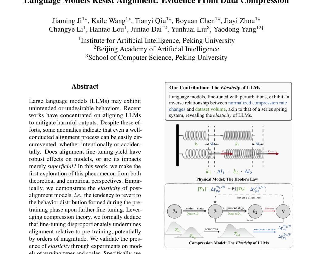
Figure 1: The Elasticity of Language Models. The change in normalized compression rates ({{\color[rgb]{0.1836,0.332,0.5938}\Delta\gamma_{p_{{\bm{\theta}}}}^{\mathcal{D}_{i}/\mathcal{D}}}}) and the dataset volume ({\color[rgb]{0.3281,0.5117,0.207}|\mathcal{D}_{i}|}) follows an inverse proportionality law after perturbations, which is akin to the relationship between spring deformation ({\color[rgb]{0.1836,0.332,0.5938}\Delta l_{i}}) and stiffness ({\color[rgb]{0.3281,0.5117,0.207}k_{i}}) in coupled springs. We conjecture that the elasticity causes language models to resist alignment, enabling the possibility of inverse alignment.

图 1：语言模型的弹性。 扰动后，归一化压缩率变化（{{\color[rgb]{0.1836,0.332,0.5938}\Delta\gamma_{p_{{\bm{\theta}}}}^{\mathcal{D}_{i}/\mathcal{D}}}}）与数据集体积（{\color[rgb]{0.3281,0.5117,0.207}|\mathcal{D}_{i}|}）呈反比，类似耦合弹簧中形变（{\color[rgb]{0.1836,0.332,0.5938}\Delta l_{i}}）与刚度（{\color[rgb]{0.3281,0.5117,0.207}k_{i}}）的关系。我们推测正是弹性使语言模型抵制对齐，并使逆向对齐成为可能。

1 Introduction

1 引言

Large language models (LLMs) have shown remarkable capabilities Achiam et al. (2023); Zhang et al. (2025). However, due to the inevitable biases and harmful content present in training datasets (Bai et al., 2022a; Ji et al., 2024c; Qian et al., 2024; Lin et al., 2025), LLMs often exhibit behaviors that deviate from human intentions, a phenomenon we refer to as model misalignment . Training-based alignment methods, including supervised fine-tuning (SFT), reinforcement learning with human feedback (RLHF) (Ouyang et al., 2022), and other derivatives Rafailov et al. (2024); Bai et al. (2022b); Lee et al. (2023); Gulcehre et al. (2023); Dong et al. (2023); Xiong et al. (2024); Li et al. (2023); Zhou et al. (2023); Zhou et al. (2025); Ji et al. (2024a), are the dominant approaches for aligning models. These methods aim to optimize model behavior by rejecting harmful distributions, ensuring LLMs remain consistent with human intentions and values Ji et al. (2023); Casper et al. (2023).

大语言模型（LLM）已展现出卓越能力 Achiam et al. (2023); Zhang et al. (2025)。但由于训练数据中不可避免的偏见与有害内容 (Bai et al., 2022a; Ji et al., 2024c; Qian et al., 2024; Lin et al., 2025)，LLM 常表现出偏离人类意图的行为，我们称之为 模型不对齐 。基于训练的对齐方法——包括监督微调（SFT）、基于人类反馈的强化学习（RLHF）(Ouyang et al., 2022) 及其他衍生 Rafailov et al. (2024); Bai et al. (2022b); Lee et al. (2023); Gulcehre et al. (2023); Dong et al. (2023); Xiong et al. (2024); Li et al. (2023); Zhou et al. (2023); Zhou et al. (2025); Ji et al. (2024a)——是对齐模型的主流途径。这些方法通过拒绝有害分布来优化模型行为，使 LLM 与人类意图与价值保持一致 Ji et al. (2023); Casper et al. (2023)。

However, these alignment methods do not truly penetrate the model representations but merely perform superficial alignment Qi et al. (2024a); Cohen et al. (2024); Wen et al. (2024). Recent studies have shown that highly safety-aligned models can become unsafe again with minimal fine-tuningYang et al. (2023b); Zhou et al. (2024). Furthermore, fine-tuning aligned LLMs on non-malicious datasets may also weaken models’ safety mechanisms Qi et al. (2024a); Jain et al. (2023).

然而，这些对齐方法并未真正深入模型表征，而只是做 表层对齐 Qi et al. (2024a); Cohen et al. (2024); Wen et al. (2024)。近期研究表明，高度安全对齐的模型只需极少微调即可再次变得不安全 Yang et al. (2023b); Zhou et al. (2024)。此外，在非恶意数据集上微调已对齐 LLM，也可能削弱其安全机制 Qi et al. (2024a); Jain et al. (2023)。

Why is alignment so fragile?

为什么对齐如此脆弱？

In this work, we make the first exploration of the possible mechanism behind the counterintuitive phenomenon: the existence of an alignment resistance mechanism in language models. This mechanism may limit the alignment process of LLMs to superficial adjustments. It could allow the reversal or revocation of alignment through a series of technical measures, a concept we refer to as inverse alignment . What drives language models to resist alignment? How does this mechanism lead to inverse alignment ? Our key contributions are summarized as follows:

本文首次探索这一反直觉现象背后可能的机制：语言模型中存在对齐阻力机制。该机制可能把 LLM 的对齐过程限制在表层调整，并允许通过一系列技术手段逆转或撤销对齐——我们称之为 逆向对齐 。是什么驱使语言模型抵制对齐？该机制如何导致 逆向对齐 ？主要贡献如下：

• (Phenomenon) We uncover that language models exhibit elasticity, as illustrated in Figure 1 and Theorem 4.2. It encompasses resistance: pre-trained models tend to retain their original distribution; and rebound: the deeper alignment of models, the faster they return to the pre-trained distribution under reverse finetuning. Moreover, The model’s change in compression rates {\color[rgb]{0.1836,0.332,0.5938}\Delta\gamma_{p_{\bm{\theta}}}^{\mathcal{D}_{i}/\mathcal{D}}} across different datasets is inversely proportional to their sizes {\color[rgb]{0.3281,0.5117,0.207}|\mathcal{D}_{i}|}, which is analogous to the deformation behavior of a series of springs, as illustrated in Section 4.3.

• （现象） 我们揭示语言模型具有弹性，如图 1 与定理 4.2 所示。它包含阻力：预训练模型倾向于保留其原始分布；以及反弹：模型对齐越深，在反向微调下越快回到预训练分布。此外，模型在不同数据集上的压缩率变化 {\color[rgb]{0.1836,0.332,0.5938}\Delta\gamma_{p_{\bm{\theta}}}^{\mathcal{D}_{i}/\mathcal{D}}} 与数据集大小 {\color[rgb]{0.3281,0.5117,0.207}|\mathcal{D}_{i}|} 成反比，类似串联弹簧的形变行为，见第 4.3 节。

• (Mechanism) We systematically model the training and alignment process of language models through compression theorem, as detailed in Section 3.2. We elaborate on the compression protocol of language models to explore their training and alignment processes, laying a foundation for subsequent research on elasticity .

• （机制） 我们借助压缩定理系统建模语言模型的训练与对齐过程，详见第 3.2 节。我们阐述语言模型的压缩协议以探讨其训练与对齐，为后续 弹性 研究奠基。

• (Validation) We experimentally observe consistent resistance and rebound phenomena across various LLMs, as detailed in Section 5. This highlights the universality of elasticity and the need for systematic approaches to achieve robust and deep alignment.

• （验证） 我们在多种 LLM 上实验观察到一致的 阻力 与 反弹 现象，详见第 5 节。这凸显 弹性 的普遍性，以及需要系统方法以实现稳健、深入的对齐。

2 Related Work

2 相关工作

The Fragility of LLMs Alignment Pre-trained LLMs often generate offensive content. Recent initiatives Ouyang et al. (2022); Bai et al. (2022a); Yang et al. (2024) have aimed to align these models to minimize harmful outputs Yang et al. (2023a); Cui et al. (2024). However, research indicates that even well-aligned models can be compromised easily, and fine-tuning them on non-malicious datasets might unintentionally impair their safety mechanisms Yang et al. (2023b); Qi et al. (2024b); Hubinger et al. (2024); Dong et al. (2024). Moreover, recent study reveals that models selectively adhere to training objectives during the training phase to preserve their inherent preferences Greenblatt et al. (2024); Lang et al. (2024); Park et al. (2024). Why is alignment so fragile? Wei et al. (2024) use weight attribution to separate safety-critical and utility-related regions at both neuron and rank levels. Qi et al. (2024a) propose the concept of shallow safety alignment, arguing that safety alignment should reach beyond surface-level tokens to shape the model’s internal mechanisms.

LLM 对齐的脆弱性 预训练 LLM 常生成冒犯性内容。近期倡议 Ouyang et al. (2022); Bai et al. (2022a); Yang et al. (2024) 旨在对齐这些模型以减少有害输出 Yang et al. (2023a); Cui et al. (2024)。但研究表明，即便对齐良好的模型也易被破坏，且在非恶意数据上微调也可能无意损害安全机制 Yang et al. (2023b); Qi et al. (2024b); Hubinger et al. (2024); Dong et al. (2024)。此外，近期研究揭示模型在训练阶段会选择性地遵循训练目标以保留固有偏好 Greenblatt et al. (2024); Lang et al. (2024); Park et al. (2024)。为什么对齐如此脆弱？Wei et al. (2024) 用权重归因在神经元与秩两个层面分离安全关键区域与效用相关区域。Qi et al. (2024a) 提出浅层安全对齐概念，主张安全对齐应超越表层 token，塑造模型内部机制。

3 What is Elasticity ?

3 什么是 弹性 ？

We discover that language models exhibit elasticity, which leads to resistance to alignment. In this section, we formally introduce the definition of elasticity, along with the compression theory tools used in the analysis. Firstly, we review the training alignment objective and the compression theorem.

我们发现语言模型具有弹性，从而导致对齐阻力。本节形式引入 弹性 的定义，以及分析中使用的压缩理论工具。首先回顾训练对齐目标与压缩定理。

3.1 Preliminaries

3.1 预备知识

\mathcal{L}_{\text{PT}}({\bm{\theta}};\mathcal{D}_{\text{PT}})

\mathcal{L}_{\text{PT}}({\bm{\theta}};\mathcal{D}_{\text{PT}})

\displaystyle\mathcal{L}_{\text{PT}}({\bm{\theta}};\mathcal{D}_{\text{PT}})=-\mathbb{E}_{({\bm{x}},x_{N})\sim\mathcal{D}_{\mathrm{PT}}}\left[\log p_{{\bm{\theta}}}\left(x_{N}\big|{\bm{x}}\right)\right],

{\bm{x}}=(x_{0},\cdots,x_{N-1})

{\bm{x}}=(x_{0},\cdots,x_{N-1})

\mathcal{D}_{\mathrm{SFT}}=\left\{\left({\bm{x}}^{i},{\bm{y}}^{i}\right)\right\}_{i=1}^{N}

\mathcal{D}_{\mathrm{SFT}}=\left\{\left({\bm{x}}^{i},{\bm{y}}^{i}\right)\right\}_{i=1}^{N}

\mathcal{L}_{\text{SFT}}({\bm{\theta}};\mathcal{D}_{\text{SFT}})=-\mathbb{E}_{({\bm{x}},\bf{y)\sim\mathcal{D}_{\mathrm{SFT}}}}\left[\log p_{{\bm{\theta}}}\left({\bm{y}}\big|{\bm{x}}\right)\right].

\mathbb{E}_{({\bm{x}},\bf{y)\sim\mathcal{D}_{\text{SFT}}}}\left[\log{p_{\mathcal{D}}\left({\bm{y}}\big|{\bm{x}}\right)}\right]

\mathcal{D}_{\text{SFT}}

\mathcal{D}

\mathcal{D}

\mathcal{L}\geq H\left(\mathcal{P}_{\mathcal{D}}\right),

H\left(\mathcal{P}_{\mathcal{D}}\right)

H\left(\mathcal{P}_{\mathcal{D}}\right)

p_{{\bm{\theta}}}

p_{{\bm{\theta}}}

\mathcal{L}=\mathbb{E}_{{\bm{x}}\sim\mathcal{D}}\left[\sum_{0\leq k\leq m}-\log_{2}p_{{\bm{\theta}}}\left(x_{k}\big|x_{0,\cdots,k-1}\right)\right],

which is the current training objective of language models. Minimizing log-likelihood loss is equivalent to minimizing the compression rate when models act as a lossless compressor. Thus, optimal compression and prediction are equivalent Delétang et al. (2023); Hutter (2005). Experiments show the equivalence between large language model prediction and compression Delétang et al. (2023), and that compression performance correlates linearly with intelligence Huang et al. (2024).

这正是当前语言模型的训练目标。最小化对数似然损失等价于模型作为无损压缩器时最小化压缩率。因此，最优压缩与最优预测等价 Delétang et al. (2023); Hutter (2005)。实验显示大语言模型预测与压缩等价 Delétang et al. (2023)，且压缩性能与智能线性相关 Huang et al. (2024)。

3.2 The Compression Protocol of LLMs

3.2 LLM 的压缩协议

We aim to study the dynamic changes in language models during training and alignment. Given the equivalence between language model training and data compression Delétang et al. (2023), a feasible modeling approach is to treat the language model as a lossless compression protocol. The process of training and aligning the model on different datasets can be equivalently viewed as the joint compression of these datasets by the protocol. The model’s compression rate on various datasets serves as a surrogate metric for the loss during training and alignment. In this section, we detail the modeling specifics of this compression protocol.

我们旨在研究语言模型在训练与对齐中的动态变化。鉴于语言模型训练与数据压缩的等价性 Delétang et al. (2023)，可行建模是把语言模型视为无损压缩协议。在不同数据集上训练与对齐，可等价视为协议对这些数据集的联合压缩。模型在各数据集上的压缩率可作为训练与对齐损失的代理指标。本节详述该压缩协议的建模细节。

Considering the impact of tokenization on compression rate, we use tokenized sequences as input and output modalities. For simplicity, we assume the tokenized vocabulary consists of only binary tokens (specifically 0/1).

考虑到 tokenization 对压缩率的影响，我们用 token 化序列作为输入输出模态。为简化，假设 token 词表仅含二元 token（具体为 0/1）。

\mathcal{T}

\mathcal{T}

\mathcal{T}

\mathcal{T}

Based on the above assumption, we can define the compression protocol during the model training and alignment process.

基于上述假设，我们可以定义模型训练与对齐过程中的压缩协议。

Definition 3.3 (The Compression Protocal) . Due to the optimality and losslessness of Huffman coding Huffman (1952), the compression protocol ensures optimal compression while preserving losslessness. We can therefore calculate the model’s ideal code length and other information-theoretic metrics based on the protocol.

定义 3.3 （压缩协议）。 由于 Huffman 编码 Huffman (1952) 的最优性与无损性，该压缩协议在保持无损的同时保证最优压缩。因此我们可据此计算模型的理想码长及其他信息论度量。

\displaystyle\mathbb{E}\left[\mathcal{L}_{p_{{\bm{\theta}}}}\left({\bm{x}}\right)\right]=\left\lceil\frac{\big|{\bm{x}}\big|}{d}\right\rceil\left\lceil-\sum_{l=1}^{d}\sum_{j=1}^{2^{l-1}}p_{lj}\log{p_{lj}}\right\rceil

\displaystyle\mathbb{E}\left[\mathcal{L}_{p_{{\bm{\theta}}}}\left({\bm{x}}\right)\right]=\left\lceil\frac{\big|{\bm{x}}\big|}{d}\right\rceil\left\lceil-\sum_{l=1}^{d}\sum_{j=1}^{2^{l-1}}p_{lj}\log{p_{lj}}\right\rceil

N

N

\displaystyle p_{lj}^{\mathcal{D}}=\frac{\sum_{i=1}^{N}p_{l}^{\mathcal{D}_{i}}\big|\mathcal{D}_{i}\big|}{\sum_{i=1}^{N}\big|\mathcal{D}_{i}\big|},

p_{lj}^{\mathcal{D}_{i}}

p_{lj}^{\mathcal{D}_{i}}

\displaystyle\gamma_{p_{{\bm{\theta}}}}^{\mathcal{D}_{i}} \\ \displaystyle=\mathbb{E}_{{\bm{x}}\sim\mathcal{P}_{i}}\left[\frac{\mathbb{E}_{{\bm{x}}\sim\mathcal{P}_{i}}\left[\mathcal{L}_{p_{{\bm{\theta}}}}^{\mathcal{D}_{i}}({\bm{x}})\right]}{\big|{\bm{x}}\big|}\right] \\ \displaystyle=\Theta\left(-\frac{\sum_{l=1}^{d}\sum_{j=1}^{2^{l-1}}p_{lj}^{\mathcal{D}_{i}}\log{p_{lj}^{\mathcal{D}}}}{d}\right).

Here, the compression rate is defined as the compressed encoding length divided by the original length Delétang et al. (2023) and ensures consistency between the training and compression objective, which means that minimizing the training loss is equivalent to minimizing the compression rate. Please see Appendix A for more details.

此处压缩率定义为压缩编码长度除以原始长度 Delétang et al. (2023)，并保证训练目标与压缩目标一致，即最小化训练损失等价于最小化压缩率。更多细节见附录 A。

3.3 The Formal Definition of Elasticity

3.3 弹性 的形式定义

To formalize inverse alignment and elasticity, we provide precise definitions of these concepts.

为形式化 逆向对齐 与 弹性 ，我们给出这些概念的精确定义。

p_{{\bm{\theta}}_{1}}\xmapsto{g(\mathcal{D}_{b})}p_{{\bm{\theta}}_{0}^{\prime}}\text{~and~}\rho(p_{{\bm{\theta}}_{0}^{\prime}},p_{{\bm{\theta}}_{0}})\leq\epsilon_{0}.

p_{{\bm{\theta}}_{1}}\xmapsto{g(\mathcal{D}_{b})}p_{{\bm{\theta}}_{0}^{\prime}}\text{~and~}\rho(p_{{\bm{\theta}}_{0}^{\prime}},p_{{\bm{\theta}}_{0}})\leq\epsilon_{0}.

\rho

\rho

4 Why Elasticity Affects Alignment?

4 为什么 弹性 影响对齐？

By now, we hope to have convinced the reader of the concept of compression modeling in language models’ training and alignment. In the following, we apply this to analyze language models’ training and alignment process, focusing on the underlying reasons that lead the model to alignment resistance.

至此，我们希望已说服读者接受用压缩建模语言模型训练与对齐的概念。接下来用它分析语言模型的训练与对齐过程，聚焦导致模型产生对齐阻力的底层原因。

In Figure 1, we have already presented the theorem of elasticity : when subject to fine-tuning perturbations, language models tend to retain the distribution associated with larger datasets while rejecting that of smaller ones. But why elasticity resists alignment? Is there a corresponding elastic invariant? How does elasticity make inverse alignment possible? In this section, we will formalize elasticity of language models and analyze the impact of elasticity on the model’s behavior.

图 1 中我们已给出 弹性 定理：在微调扰动下，语言模型倾向于保留与更大数据集相关的分布，而拒绝更小数据集的分布。但为什么 弹性 会抵制对齐？是否存在相应的 弹性 不变量？ 弹性 如何使 逆向对齐 成为可能？本节将形式化语言模型的 弹性 ，并分析其对模型行为的影响。

4.1 Formal Derivation of Elasticity

4.1 弹性 的形式推导

\mathcal{D}_{p}

\mathcal{D}_{p}

N

N

\gamma_{p_{{\bm{\theta}}}}^{\mathcal{D}_{i}/\mathcal{D}}=\gamma_{p_{{\bm{\theta}}}}^{\mathcal{D}_{i}}-\log{M}, \tag{1}

M

M

The normalized compression rate allows for comparing the model’s compression performance across different datasets. The smaller the normalized compression rate of a dataset, the better the model’s compression performance on the dataset.

归一化压缩率便于比较模型在不同数据集上的压缩表现。某数据集的归一化压缩率越小，模型在该数据集上的压缩越好。

With this definition in hand, we proceed to our main result: language models exhibit elasticity .

有了这一定义，我们给出主要结果：语言模型具有 弹性 。

Theorem 4.2(Elasticity of Language Models). $$\begin{split}\frac{d\gamma_{p_{{\bm{\theta}}}}^{\mathcal{D}{a}/\mathcal{D}}}{d,l}&=\Theta\left(-k\frac{d\gamma{p_{{\bm{\theta}}}}^{\mathcal{D}{p}/\mathcal{D}}}{d,l}\right),\\frac{d\gamma{p_{{\bm{\theta}}}}^{\mathcal{D}_{p}/\mathcal{D}}}{d,l}&<0,\frac{d\gamma_{p_{{\bm{\theta}}}}^{\mathcal{D}_{a}/\mathcal{D}}}{d,l}>0,\end{split} \tag{2}$$

Theorem 4.2(Elasticity of Language Models). $$\begin{split}\frac{d\gamma_{p_{{\bm{\theta}}}}^{\mathcal{D}{a}/\mathcal{D}}}{d,l}&=\Theta\left(-k\frac{d\gamma{p_{{\bm{\theta}}}}^{\mathcal{D}{p}/\mathcal{D}}}{d,l}\right),\\frac{d\gamma{p_{{\bm{\theta}}}}^{\mathcal{D}_{p}/\mathcal{D}}}{d,l}&<0,\frac{d\gamma_{p_{{\bm{\theta}}}}^{\mathcal{D}_{a}/\mathcal{D}}}{d,l}>0,\end{split} \tag{2}$$

\mathcal{D}_{p}

\mathcal{D}_{p}

4.2 Elasticity and Inverse Alignment

4.2 弹性 与 逆向对齐

Theorem 4.2 shows the normalized compression rate change of different datasets is inversely proportional to their sizes under perturbations. A significant size difference between the pre-training and alignment datasets causes rapid performance degradation on the alignment dataset due to the inverse relationship, often spanning several orders of magnitude.

定理 4.2 表明：扰动下不同数据集的归一化压缩率变化与其大小成反比。预训练与对齐数据集规模差异显著时，反比关系使对齐数据集上的性能快速退化，往往跨越数个数量级。

Intuitively, the model’s compression process across multiple datasets is akin to resource allocation between towns: in a region with both a large metropolis and rural villages, to maximize overall economic productivity, resources are typically allocated to the metropolis first, to leverage its scale and agglomeration effects. In other words, the metropolis/large dataset occupies a dominant position in the system.

直观上，模型跨多数据集的压缩过程类似城镇间的资源分配：一个地区既有大都市又有乡村时，为最大化整体经济产出，资源通常先投向大都市以发挥其规模与集聚效应。换言之，大都市/大数据集在系统中占据主导地位。

Therefore, the elasticity of language models makes inverse alignment possible. Due to the substantial data volume disparity between pre-training and alignment datasets, the model tends to revert to the pre-training rather than alignment distribution when subsequent perturbations occur. This indicates an inherent tendency toward inverse alignment during fine-tuning. Maximizing the impact of elasticity through well-designed perturbations will be key to achieving true inverse alignment .

因此，语言模型的 弹性 使 逆向对齐 成为可能。由于预训练与对齐数据集体积差距巨大，后续扰动发生时模型更倾向回退到预训练而非对齐分布。这表明微调中存在固有的 逆向对齐 倾向。通过精心设计的扰动最大化 弹性 影响，将是实现真正 逆向对齐 的关键。

4.3 Elasticity and the Hooke’s Law.

4.3 弹性 与胡克定律

The inverse proportionality result in Theorem 4.2 provides a potential invariant in the model training and alignment process: after perturbation, the rate of change in the compression rates of different datasets is inversely proportional to their sizes, with the absolute value of the product being a constant. This constant characterizes the impact of the perturbation on the model and indirectly describes the model’s resistance to perturbations, or its elasticity .

定理 4.2 中的反比结果提供了模型训练与对齐过程中的潜在不变量：扰动后，不同数据集压缩率变化速率与其大小成反比，乘积绝对值是常数。该常数刻画扰动对模型的影响，并间接描述模型对扰动的阻力，或其 弹性 。

F

F

F\propto{\color[rgb]{0.3281,0.5117,0.207}k_{1}}\cdot{\color[rgb]{0.1836,0.332,0.5938}\Delta l_{1}}={\color[rgb]{0.3281,0.5117,0.207}k_{2}}\cdot{\color[rgb]{0.1836,0.332,0.5938}\Delta l_{2}}\;.

l

l

F\propto{\color[rgb]{0.3281,0.5117,0.207}|\mathcal{D}_{i}|}\cdot{\color[rgb]{0.1836,0.332,0.5938}\Delta D_{\text{KL}}(\mathcal{P}_{p_{{\bm{\theta}}}}||\mathcal{P}_{\mathcal{D}_{i}})}\;, \tag{3}

where {\color[rgb]{0.1836,0.332,0.5938}\Delta D_{\text{KL}}} corresponds to {\color[rgb]{0.1836,0.332,0.5938}\Delta l} in the spring model, while {\color[rgb]{0.3281,0.5117,0.207}|\mathcal{D}|} corresponds to the spring constant {\color[rgb]{0.3281,0.5117,0.207}k}, thus leading to the elasticity of LLMs.

其中 {\color[rgb]{0.1836,0.332,0.5938}\Delta D_{\text{KL}} 对应弹簧模型中的 {\color[rgb]{0.1836,0.332,0.5938}\Delta l}，而 {\color[rgb]{0.3281,0.5117,0.207}|\mathcal{D}|} 对应劲度系数 {\color[rgb]{0.3281,0.5117,0.207}k}，从而导出 LLM 的弹性。

{\bm{\theta}}_{2}\rightarrow{\bm{\theta}}_{1}

Datasets	Base Models	${\bm{\theta}}_{2}\rightarrow{\bm{\theta}}_{1}$ vs. ${\bm{\theta}}_{1}\rightarrow{\bm{\theta}}_{2}$	${\bm{\theta}}_{3}\rightarrow{\bm{\theta}}_{2}$ vs. ${\bm{\theta}}_{2}\rightarrow{\bm{\theta}}_{3}$	${\bm{\theta}}_{3}\rightarrow{\bm{\theta}}_{1}$ vs. ${\bm{\theta}}_{1}\rightarrow{\bm{\theta}}_{3}$
Alpaca	Llama2-7B	0.1589 $\downarrow$ 0.2018 $\uparrow$	0.1953 $\downarrow$ 0.2143 $\uparrow$	0.1666 $\downarrow$ 0.2346 $\uparrow$
Llama2-13B	0.1772 $\downarrow$ 0.1958 $\uparrow$	0.2149 $\downarrow$ 0.2408 $\uparrow$	0.1835 $\downarrow$ 0.2345 $\uparrow$
Llama3-8B	0.2540 $\downarrow$ 0.2573 $\uparrow$	0.2268 $\downarrow$ 0.3229 $\uparrow$	0.2341 $\downarrow$ 0.2589 $\uparrow$
Truthful	Llama2-7B	0.1909 $\downarrow$ 0.2069 $\uparrow$	0.1719 $\downarrow$ 0.1721 $\uparrow$	0.2011 $\downarrow$ 0.2542 $\uparrow$
Llama2-13B	0.1704 $\downarrow$ 0.1830 $\uparrow$	0.1544 $\downarrow$ 0.1640 $\uparrow$	0.1825 $\downarrow$ 0.2429 $\uparrow$
Llama3-8B	0.2118 $\downarrow$ 0.2256 $\uparrow$	0.2100 $\downarrow$ 0.2173 $\uparrow$	0.2393 $\downarrow$ 0.2898 $\uparrow$
Safe	Llama2-7B	0.2730 $\downarrow$ 0.2809 $\uparrow$	0.2654 $\downarrow$ 0.2691 $\uparrow$	0.2845 $\downarrow$ 0.2883 $\uparrow$
Llama2-13B	0.2419 $\downarrow$ 0.2439 $\uparrow$	0.2320 $\downarrow$ 0.2327 $\uparrow$	0.2464 $\downarrow$ 0.2606 $\uparrow$
Llama3-8B	0.2097 $\downarrow$ 0.2156 $\uparrow$	0.2008 $\downarrow$ 0.2427 $\uparrow$	0.2277 $\downarrow$ 0.2709 $\uparrow$

{\bm{\theta}}_{2}\rightarrow{\bm{\theta}}_{1}

Datasets	Base Models	${\bm{\theta}}_{2}\rightarrow{\bm{\theta}}_{1}$ vs. ${\bm{\theta}}_{1}\rightarrow{\bm{\theta}}_{2}$	${\bm{\theta}}_{3}\rightarrow{\bm{\theta}}_{2}$ vs. ${\bm{\theta}}_{2}\rightarrow{\bm{\theta}}_{3}$	${\bm{\theta}}_{3}\rightarrow{\bm{\theta}}_{1}$ vs. ${\bm{\theta}}_{1}\rightarrow{\bm{\theta}}_{3}$
Alpaca	Llama2-7B	0.1589 $\downarrow$ 0.2018 $\uparrow$	0.1953 $\downarrow$ 0.2143 $\uparrow$	0.1666 $\downarrow$ 0.2346 $\uparrow$
Llama2-13B	0.1772 $\downarrow$ 0.1958 $\uparrow$	0.2149 $\downarrow$ 0.2408 $\uparrow$	0.1835 $\downarrow$ 0.2345 $\uparrow$
Llama3-8B	0.2540 $\downarrow$ 0.2573 $\uparrow$	0.2268 $\downarrow$ 0.3229 $\uparrow$	0.2341 $\downarrow$ 0.2589 $\uparrow$
Truthful	Llama2-7B	0.1909 $\downarrow$ 0.2069 $\uparrow$	0.1719 $\downarrow$ 0.1721 $\uparrow$	0.2011 $\downarrow$ 0.2542 $\uparrow$
Llama2-13B	0.1704 $\downarrow$ 0.1830 $\uparrow$	0.1544 $\downarrow$ 0.1640 $\uparrow$	0.1825 $\downarrow$ 0.2429 $\uparrow$
Llama3-8B	0.2118 $\downarrow$ 0.2256 $\uparrow$	0.2100 $\downarrow$ 0.2173 $\uparrow$	0.2393 $\downarrow$ 0.2898 $\uparrow$
Safe	Llama2-7B	0.2730 $\downarrow$ 0.2809 $\uparrow$	0.2654 $\downarrow$ 0.2691 $\uparrow$	0.2845 $\downarrow$ 0.2883 $\uparrow$
Llama2-13B	0.2419 $\downarrow$ 0.2439 $\uparrow$	0.2320 $\downarrow$ 0.2327 $\uparrow$	0.2464 $\downarrow$ 0.2606 $\uparrow$
Llama3-8B	0.2097 $\downarrow$ 0.2156 $\uparrow$	0.2008 $\downarrow$ 0.2427 $\uparrow$	0.2277 $\downarrow$ 0.2709 $\uparrow$

5 How Elasticity Resists Alignment?

5 弹性 如何抵制对齐？

In the previous sections, we proved that LLMs have elasticity . This section will analyze two specific phenomenons of it:

前几节我们证明了 LLM 具有 弹性 。本节分析其两个具体现象：

• Resistance for Pre-Trained Models. Models tend to maintain the original distribution and resist alignment;

• 预训练模型的阻力。 模型倾向于维持原始分布并抵制对齐；

• Rebound for Post-Trained Models. Fine-tuning in the opposite direction of post-training (e.g., safe vs . unsafe) causes post-trained models to return quickly to the pre-training distribution.

• 后训练模型的反弹。 沿后训练相反方向微调（例如安全 vs. 不安全）会使后训练模型迅速回到预训练分布。

5.1 Existence of Language Models’ Resistance

5.1 语言模型 阻力 的存在性

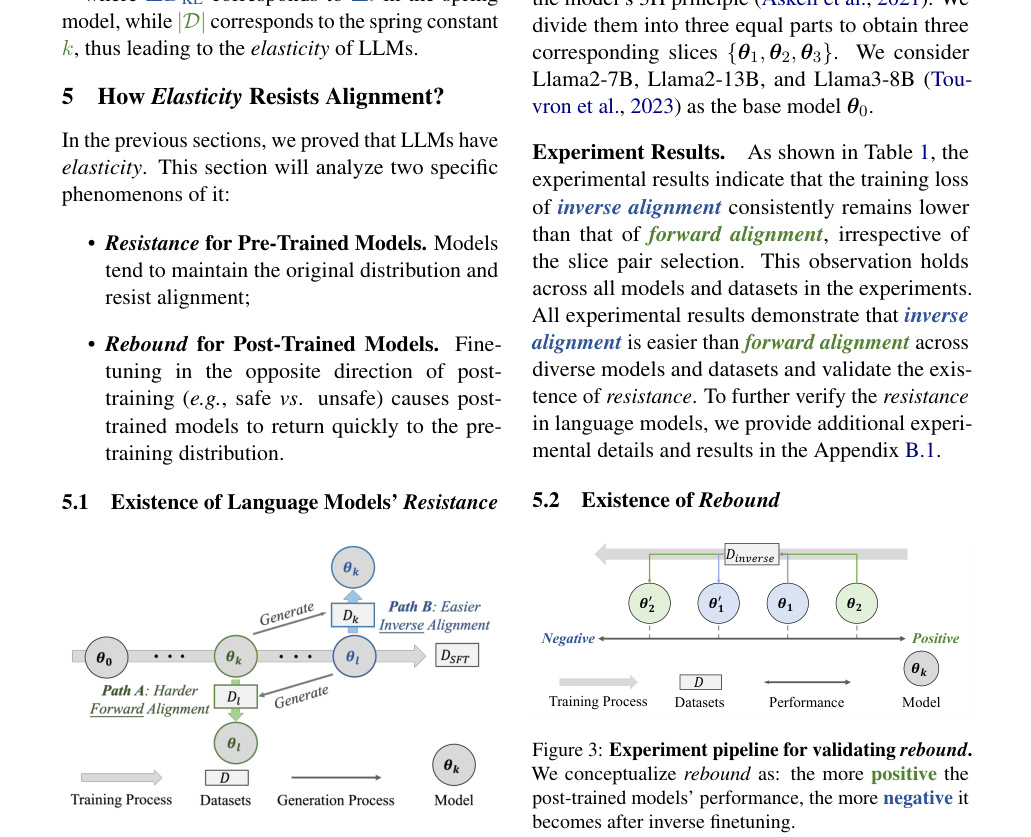
Figure 2: Experiment pipeline for validating resistance . We conceptualize resistance as: inverse alignment is easier than forward alignment .

图 2： 验证 阻力 的实验流水线 。 我们将 阻力 概念化为： 逆向对齐 比 正向对齐 更容易。

{\bm{\theta}}_{0}

{\bm{\theta}}_{0}

\{{\bm{\theta}}_{1},{\bm{\theta}}_{2},{\bm{\theta}}_{3}\}

\{{\bm{\theta}}_{1},{\bm{\theta}}_{2},{\bm{\theta}}_{3}\}

Experiment Results. As shown in Table 1, the experimental results indicate that the training loss of inverse alignment consistently remains lower than that of forward alignment, irrespective of the slice pair selection. This observation holds across all models and datasets in the experiments. All experimental results demonstrate that inverse alignment is easier than forward alignment across diverse models and datasets and validate the existence of resistance . To further verify the resistance in language models, we provide additional experimental details and results in the Appendix B.1.

实验结果。 如表 1，实验结果表明：无论选择哪对切片， 逆向对齐 的训练损失始终低于 正向对齐 。该观察在实验中的全部模型与数据集上成立。所有结果都表明：跨多样模型与数据集， 逆向对齐 比 正向对齐 更容易，从而验证了 阻力 的存在。为进一步验证语言模型中的 阻力 ，附录 B.1 提供更多实验细节与结果。

5.2 Existence of Rebound

5.2 反弹 的存在性

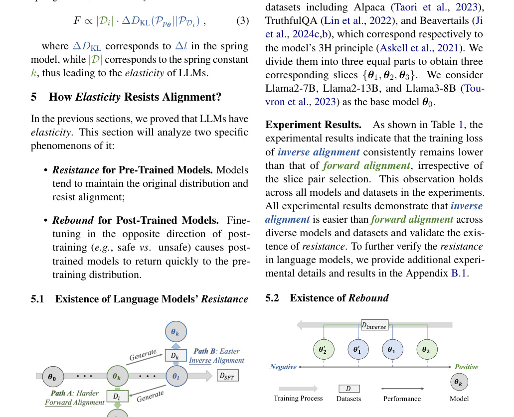
Figure 3: Experiment pipeline for validating rebound . We conceptualize rebound as: the more positive the post-trained models’ performance, the more negative it becomes after inverse finetuning.

图 3： 验证 反弹 的实验流水线 。 我们将 反弹 概念化为：后训练模型表现越 正 ，经逆向微调后越 负 。

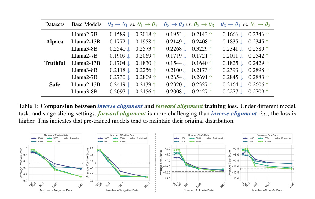
Figure 4: Experimental results for validating the existence of rebound (left: IMDb, right: Beavertails). The left part of each sub-figure is the performance of Gemma-2B while the right is Llama2-7B, respectively. Models trained with more positive data initially perform better but perform worse after fine-tuning with negative data.

图 4： 验证 反弹 存在性的实验结果（左：IMDb，右：Beavertails） 。 各子图左侧为 Gemma-2B，右侧为 Llama2-7B。用更多 正 数据训练的模型起初表现更好，但用 负 数据微调后表现更差。

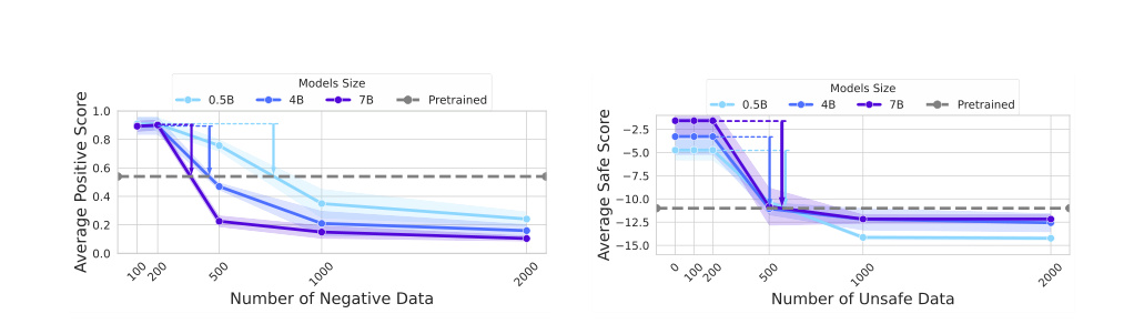
Figure 5: Experimental results for validating rebound increases with model size (left: IMDb, right: Beavertails). All single line covers positive data volume settings as Figure 4, with shadow denoting std. As the model size increases, the performance of the aligned model deteriorates more rapidly after fine-tuning with negative data.

图 5： 验证 反弹 随模型规模增大的实验结果（左：IMDb，右：Beavertails） 。 每条线覆盖如图 4 的正数据量设定，阴影为标准差。随模型变大，对齐模型在用 负 数据微调后性能下降更快。

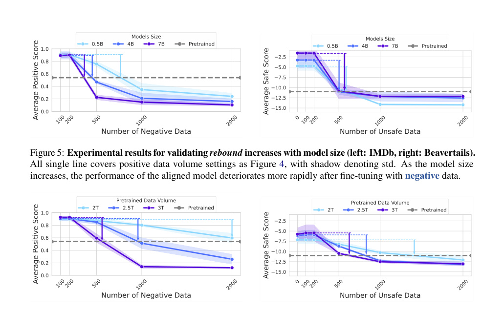
Figure 6: Experimental results for validating rebound increases with pre-training data volume. (left: IMDb, right: Beavertails). Each line covers positive data settings as Figure 4, with shadow denoting std. As pre-training data volume increases, aligned model performance deteriorates more rapidly after fine-tuning with negative data.

图 6： 验证 反弹 随预训练数据量增大的实验结果（左：IMDb，右：Beavertails） 。 每条线覆盖如图 4 的正数据设定，阴影为标准差。随预训练数据量增加，对齐模型在用 负 数据微调后性能下降更快。

\{{\bm{\theta}}_{1},{\bm{\theta}}_{2},...,{\bm{\theta}}_{n}\}

{\bm{\theta}}_{0}

Tasks and Datasets. We select two tasks: positive generation and single-turn safe conversation. For the former, we use the data classified as positive or negative in the IMDb dataset (Maas et al., 2011). Referring to Rafailov et al. (2024), we use the first 2-8 tokens of each complete text as a prompt for LLMs to generate the subsequent content. For the latter, we use the data classified as safe and unsafe in Beavertails (Ji et al., 2024c). We organized the positive sample sizes into {1000, 2000, 5000, 10000}, while the negative sample sizes, were divided into {100, 200, 500, 1000, 2000}.

任务与数据集。 我们选择两个任务：正向生成与单轮安全对话。前者使用 IMDb 数据集 (Maas et al., 2011) 中标为正或负的数据。参考 Rafailov et al. (2024)，用每段完整文本的前 2-8 个 token 作为提示，让 LLM 生成后续内容。后者使用 Beavertails (Ji et al., 2024c) 中标为安全与不安全的数据。正样本规模设为 {1000, 2000, 5000, 10000}，负样本规模分为 {100, 200, 500, 1000, 2000}。

Evaluation and Metrics. We collect the model’s responses on the reserved test prompts. Then we use score models provided by existing research to complete the performance evaluation. For positive style generation, we refer to Rafailov et al. (2024) and use the Sentiment Roberta model (Hartmann et al., 2023) to classify the responses, taking the proportion of all responses classified as positive as the model score. For single-turn safe dialogue, we use the cost model (Dai et al., 2024) to score the safety of each response, using the average score of all responses as the model score.

评测与指标。 我们收集模型在留出测试提示上的回答，再用已有研究提供的打分模型完成性能评估。对正向风格生成，参考 Rafailov et al. (2024)，用 Sentiment Roberta 模型 (Hartmann et al., 2023) 分类回答，以被判为正的回答比例作为模型分数。对单轮安全对话，用代价模型 (Dai et al., 2024) 为每条回答打安全分，以全部回答的平均分作为模型分数。

Experiment Results. We evaluate the rebound phenomenon on Llama2-7B (Touvron et al., 2023) and Gemma-2B (Team et al., 2024). The experimental results in Figure 4 show that, for models fine-tuned with a larger amount of positive sample data, their performance drops quicker under only a small amount of negative sample fine-tuning. Subsequently, the performance decline slows down and tends to stabilize. This result also confirms the previous conclusion: the initial rapid decline of model’s performance is due to rebound, as the model is far from the pre-trained distribution; while the later stabilization of the countermeasure is due to resistance, as the model is already close to the pre-trained distribution.

实验结果。 我们在 Llama2-7B (Touvron et al., 2023) 与 Gemma-2B (Team et al., 2024) 上评估 反弹 现象。图 4 结果表明：用更多正样本微调的模型，在仅用少量负样本微调时性能下降更快；随后下降变缓并趋于稳定。该结果也印证前述结论：性能起初快速下降是由于 反弹 ——模型远离预训练分布；后期对抗趋于稳定是由于 阻力 ——模型已接近预训练分布。

To assess the generalizability of the rebound phenomenon, we perform additional ablation studies focusing on alignment algorithms, evaluation metrics, and fine-tuning directions. The results consistently validate the presence of the rebound phenomenon across language models. Further experimental details are available in Appendix B.2.

为评估 反弹 现象的泛化性，我们针对对齐算法、评测指标与微调方向做额外消融。结果一致验证语言模型中存在 反弹 现象。更多实验细节见附录 B.2。

5.3 Internal Factor of Rebound

5.3 反弹 的内部因素

We conduct an in-depth analysis of the internal factors affecting the rebound phenomenon since it is crucial for the robustness of LLMs alignment. In particular, we investigate how model parameter scale and the amount of pre-training data influence rebound . Owing to space constraints, further experimental analyses are included in Appendix B.3.

由于对 LLM 对齐稳健性至关重要，我们对影响 反弹 现象的内部因素做深入分析。特别地，我们考察模型参数规模与预训练数据量如何影响 反弹 。因篇幅限制，更多实验分析见附录 B.3。

Rebound Increases with Model Size. To investigate how the rebound phenomenon varies with model size, we conducted experiments on Qwen models (Bai et al., 2023) with parameter scales of 0.5B, 4B, and 7B. The experimental results in Figure 5 show that as the model parameter size increases, the initial performance decline due to negative data fine-tuning is faster, while the subsequent decline is slower. This indicates that as the parameter size increases, there is an increase in rebound in response to both positive and negative data, further suggesting a positive correlation between model elasticity and parameter scale.

反弹 随模型规模增大。 为考察 反弹 如何随模型规模变化，我们在参数规模为 0.5B、4B 与 7B 的 Qwen 模型 (Bai et al., 2023) 上实验。图 5 结果显示：随参数规模增大，负数据微调导致的初期性能下降更快，后续下降更慢。这表明随参数增大，对正负数据的 反弹 都增强，进一步提示模型 弹性 与参数规模正相关。

Rebound Increases with Pre-training Data Volume. To verify that rebound increases with the growth of pre-training data, we vary pre-training slices (2.0T, 2.5T, and 3.0T) released by TinyLlama (Zhang et al., 2024a) and conduct the same experiment. As shown in Figure 6, when the pre-training data volume increases, the initial performance decline due to negative data fine-tuning is faster, while the subsequent decline is slower. It demonstrates that larger pre-training data volumes reinforce the rebound of LLMs, which is consistent with the inference proposed in Theorem 4.2.

反弹 随预训练数据量增大。 为验证 反弹 随预训练数据增长而增强，我们变换 TinyLlama (Zhang et al., 2024a) 发布的预训练切片（2.0T、2.5T 与 3.0T）并做相同实验。如图 6，预训练数据量增大时，负数据微调导致的初期性能下降更快，后续下降更慢。这表明更大预训练数据量强化 LLM 的 反弹 ，与定理 4.2 的推断一致。

6 Conclusion and Outlook

6 结论与展望

Our work uncovers a possible mechanism underlying the fragility of alignment: the elasticity of language models. We demonstrate that upon perturbation, the normalized compression rate of language models changes inversely with dataset size, making them more inclined to retain pre-training distributions while forgetting alignment distributions, thus resisting alignment. Through extensive experiments, we validate the universality of this elasticity effect, observing that the elasticity strengthens as model size and pre-training data volume scale up. Fundamentally, our findings support a core assertion: language models exhibit elasticity, and thereby inherently resist alignment.

我们的工作揭示对齐脆弱性背后一种可能机制：语言模型的 弹性 。我们证明：扰动后，语言模型归一化压缩率变化与数据集大小成反比，使它们更倾向保留预训练分布而遗忘对齐分布，从而抵制对齐。通过大量实验，我们验证该 弹性 效应的普遍性，并观察到随模型规模与预训练数据量扩大， 弹性 增强。从根本上，我们的发现支持一个核心论断：语言模型具有 弹性 ，因而内在地抵制对齐。

6.1 Limitations

6.1 局限

Theory-wise, the primary limitation of our work is our specification of the mass distribution (Assumption A.7), and empirical studies on the exact form of this distribution shall be valuable. Experiment-wise, we have not systematically validated elasticity throughout the entire lifecycle of pre-training and alignment phases due to cost constraints. In future works, we plan to focus on whether this phenomenon is universally applicable, such as in multimodal models (Ji et al., 2024d; Huh et al., 2024). Additionally, we aim to theoretically uncover the relationship between model elasticity and scaling laws (Kaplan et al., 2020; Xiao et al., 2024), specifically determining the amount of training data required for elasticity to manifest and quantitatively analyzing whether elasticity intensifies as model parameters and pre-training data volume increase.

理论上，本文的主要局限是对 质量分布 的设定（假设 A.7），对该分布确切形式的实证研究将很有价值。实验上，因成本限制，我们未能在预训练与对齐全生命周期系统验证 弹性 。未来工作计划关注该现象是否普遍适用，例如在多模态模型中 (Ji et al., 2024d; Huh et al., 2024)。此外，我们希望从理论上揭示模型 弹性 与 缩放律 (Kaplan et al., 2020; Xiao et al., 2024) 的关系，具体确定 弹性 显现所需的训练数据量，并定量分析随模型参数与预训练数据量增加， 弹性 是否增强。

6.2 Broader Impacts

6.2 更广泛影响

Rethinking Fine-tuning and Model Weight from Resist Alignment. Alignment fine-tuning methods aim to efficiently adjust the distribution of LLMs with minimal data to enhance their safety mechanisms. However, current alignment algorithms for language models may rely on optimization shortcuts, leading to local optima, while lacking involvement with the intrinsic mechanisms of the model (Qi et al., 2024a). From the perspective of language models’ elasticity, we require more robust alignment methods to ensure that modifications to model parameters extend beyond superficial changes Qi et al. (2024a); Cohen et al. (2024), thereby preventing the emergence of more effective inverse alignment techniques that could give rise to extreme misalignment risks such as deceptive adversarial alignment (IDAIS-Beijing, 2024; Bengio et al., 2025; Marks et al., 2025; Baker et al., 2025) or alignment faking (Greenblatt et al., 2024). Although methods such as data cleansing during the training phase have proven to be an effective strategy for improving the malleability of a language model’s final distribution He et al. (2024); Qi et al. (2024b), such approaches are not particularly cost-effective and feasible. In Appendix C.2, we provide a preliminary discussion of practical steps based on elasticity to mitigate inverse alignment risks, and we look forward to future research and practical developments grounded in elasticity, which will enable the design of more robust alignment algorithms Revel et al. (2024); Zhang et al. (2024b); Chen et al. (2024); Sheshadri et al. (2024); Liu et al. (2024); Li et al. (2025), ultimately achieving true and reliable alignment for LLMs.

从抵制对齐重新思考微调与模型权重。 对齐微调方法旨在用最少数据高效调整 LLM 分布以增强安全机制。但当前语言模型对齐算法可能依赖优化捷径，陷入局部最优，并缺乏对模型内在机制的介入 (Qi et al., 2024a)。从语言模型 弹性 视角看，我们需要更稳健的对齐方法，确保对模型参数的修改超越表层变化 Qi et al. (2024a); Cohen et al. (2024)，从而防止更有效的 逆向对齐 技术出现，避免欺骗性对抗对齐 (IDAIS-Beijing, 2024; Bengio et al., 2025; Marks et al., 2025; Baker et al., 2025) 或对齐伪装 (Greenblatt et al., 2024) 等极端不对齐风险。虽有训练期数据清洗等已被证明能改善语言模型最终分布可塑性的策略 He et al. (2024); Qi et al. (2024b)，此类方法并不特别划算或可行。附录 C.2 基于 弹性 初步讨论缓解 逆向对齐 风险的实践步骤；我们期待未来基于 弹性 的研究与实践，设计更稳健的对齐算法 Revel et al. (2024); Zhang et al. (2024b); Chen et al. (2024); Sheshadri et al. (2024); Liu et al. (2024); Li et al. (2025)，最终实现真正可靠的 LLM 对齐。

Rethinking Open-sourcing from Elasticity of LLMs. Open-sourcing is a double-edged sword Seger et al. (2023); Anwar et al. (2024); Kukreja et al. (2024). The public release of model weights enables the technical community to quickly identify and address potential vulnerabilities and conduct large-scale research on broad safety concerns (Touvron et al., 2023). These efforts collectively help sustain a balanced offence-defense dynamic (Jervis, 1978; Garfinkel and Dafoe, 2021) in the open-source environment and improve model security (Eiras et al., 2024). However, the risk of misuse associated with open-sourcing models is inevitable (Seger et al., 2023). Malicious fine-tuning of open-source models (Urbina et al., 2022; Sandbrink, 2023) and the use of the open-source models to facilitate system jailbreaks (Zou et al., 2023) can pose serious threats to public safety (Goldstein et al., 2023; Reuel et al., 2024). At present, the open-sourcing of powerful language models relies on safety alignment and rigorous security audits (Mökander et al., 2024) to ensure responsible use. However, if advanced inverse alignment techniques become feasible, even carefully aligned and audited open-source models could be reverted to their pre-alignment states at minimal cost, drastically lowering the barrier for jailbreaking aligned models and disrupting the offense-defense balance in the open-source ecosystem Shapiro and Siegel (2010). Therefore, it is crucial to develop alignment algorithms with fine-tuning robustness. We hope that deeper insights into the elasticity mechanisms of language models will drive the advancement of untunable alignment methods, enabling models to maintain reliable safety throughout their entire lifecycle Madiega (2021).

从 LLM 弹性重新思考开源。 开源是双刃剑 Seger et al. (2023); Anwar et al. (2024); Kukreja et al. (2024)。公开发布模型权重使技术社区能快速发现并修补潜在漏洞，并开展面向广泛安全关切的大规模研究 (Touvron et al., 2023)。这些努力共同帮助在开源环境中维持攻防平衡 (Jervis, 1978; Garfinkel and Dafoe, 2021) 并改善模型安全 (Eiras et al., 2024)。但开源模型的滥用风险不可避免 (Seger et al., 2023)。对开源模型的恶意微调 (Urbina et al., 2022; Sandbrink, 2023) 以及用开源模型助推系统越狱 (Zou et al., 2023) 可能对公共安全构成严重威胁 (Goldstein et al., 2023; Reuel et al., 2024)。当前，强大语言模型的开源依赖安全对齐与严格安全审计 (Mökander et al., 2024) 以确保负责任使用。然而，若先进 逆向对齐 技术变得可行，即便经过仔细对齐与审计的开源模型也可能以极低成本回退到对齐前状态，大幅降低越狱对齐模型的门槛，并破坏开源生态中的攻防平衡 Shapiro and Siegel (2010)。因此，开发具有微调稳健性的对齐算法至关重要。我们希望对语言模型 弹性 机制的更深入洞见，推动不可微调对齐方法的发展，使模型在全生命周期保持可靠安全 Madiega (2021)。

References

参考文献

Appendix A Assumptions and Proofs

附录 A 假设与证明

Assumption A.1 (Binary Tokens) . For simplicity and without loss of generality, we assume that all datasets share a uniform token table containing only binary tokens (specifically 0/1).

假设 A.1 （二元 Token）。 为简化且不失一般性，我们假设所有数据集共享仅含二元 token（具体为 0/1）的统一 token 表。

\displaystyle\mathbb{E}\left[\mathcal{L}_{p_{{\bm{\theta}}}}\left({\bm{x}}\right)\right]=\left\lceil\frac{\big|{\bm{x}}\big|}{d}\right\rceil\left\lceil-\sum_{l=1}^{d}\sum_{j=1}^{2^{l-1}}p_{lj}\log{p_{lj}}\right\rceil,

\displaystyle\mathbb{E}\left[\mathcal{L}_{p_{{\bm{\theta}}}}\left({\bm{x}}\right)\right]=\left\lceil\frac{\big|{\bm{x}}\big|}{d}\right\rceil\left\lceil-\sum_{l=1}^{d}\sum_{j=1}^{2^{l-1}}p_{lj}\log{p_{lj}}\right\rceil,

\big|{\bm{x}}\big|\leq d

\big|{\bm{x}}\big|\leq d

\mathbb{E}\left[\mathcal{L}_{p_{{\bm{\theta}}}}\left({\bm{x}}\right)\right]=\left\lceil-\sum_{l=1}^{d}\sum_{j=1}^{2^{l-1}}p_{lj}\log{p_{lj}}\right\rceil,

d

d

sd\leq\big|{\bm{x}}\big|\leq(s+1)d

sd\leq\big|{\bm{x}}\big|\leq(s+1)d

\displaystyle\mathbb{E}_{{\bm{x}}}\left[\mathcal{L}_{p_{{\bm{\theta}}}}\left({\bm{x}}\right)\right] \\ \displaystyle=\mathbb{E}_{{\bm{x}}_{1}}\left[\mathcal{L}_{p_{{\bm{\theta}}}}\left({\bm{x}}_{1}\right)\right]+\mathbb{E}_{{\bm{x}}_{1}}\mathbb{E}_{({\bm{x}}_{2}\ldots{\bm{x}}_{s+1})}\left[\mathcal{L}_{p_{{\bm{\theta}}}}\left(\left({\bm{x}}_{2}\ldots{\bm{x}}_{s+1}\right)\right)\big|{\bm{x}}_{1}\right] \\ \displaystyle=\mathbb{E}_{{\bm{x}}_{1}}\left[\mathcal{L}_{p_{{\bm{\theta}}}}\left({\bm{x}}_{1}\right)\right]+\sum_{{\bm{x}}_{1}}p({\bm{x}}_{1})\sum_{({\bm{x}}_{2}\ldots{\bm{x}}_{s+1})}p({\bm{x}}_{2}\ldots{\bm{x}}_{s+1}\big|{\bm{x}}_{1})\cdot\mathcal{L}_{p_{{\bm{\theta}}}}\left(({\bm{x}}_{2}\ldots{\bm{x}}_{s+1})\right) \\ \displaystyle=\mathbb{E}_{{\bm{x}}_{1}}\left[\mathcal{L}_{p_{{\bm{\theta}}}}\left({\bm{x}}_{1}\right)\right]+\mathbb{E}_{({\bm{x}}_{2}\ldots{\bm{x}}_{s+1})}\left[\mathcal{L}_{p_{{\bm{\theta}}}}\left(\left({\bm{x}}_{2}\ldots{\bm{x}}_{s+1}\right)\right)\right] \\ \displaystyle=\sum_{k=1}^{s+1}\mathbb{E}_{{\bm{x}}_{k}}\left[\mathcal{L}_{p_{{\bm{\theta}}}}\left({\bm{x}}_{k}\right)\right] \\ \displaystyle=\left\lceil\frac{\big|{\bm{x}}\big|}{d}\right\rceil\left\lceil-\sum_{l=1}^{d}\sum_{j=1}^{2^{l-1}}p_{lj}\log{p_{lj}}\right\rceil,

thus the proof is completed. ∎

从而证明完成。∎

\Omega

\mathcal{D}

\mathcal{D}_{1},\ldots,\mathcal{D}_{N}

\mathcal{D}_{1},\ldots,\mathcal{D}_{N}

X_{\mathcal{D}}=\frac{\sum_{k=1}^{N}\big|\mathcal{D}_{k}\big|X_{\mathcal{D}_{k}}}{\sum_{k=1}^{N}\big|\mathcal{D}_{k}\big|},

X_{\mathcal{D}_{k}}

X_{\mathcal{D}_{k}}

\mathcal{T}_{k}^{\prime}

\mathcal{D}_{k}

\mathbb{E}_{{\bm{x}}\sim\mathcal{P}_{k}}\left[-p^{\mathcal{D}_{k}}\log{p^{\mathcal{D}}}\right]=\mathbb{E}_{X_{\mathcal{D}_{k}}\sim\mathcal{P}_{mass}^{k},X_{\mathcal{D}}\sim\mathcal{P}_{mass}}\left[-X_{\mathcal{D}_{k}}\log{X_{\mathcal{D}}}\right]+\log{M},

p^{\mathcal{D}}

p^{\mathcal{D}}

M

M

\displaystyle\mathbb{E}_{{\bm{x}}\sim\mathcal{P}_{k}}\left[-p^{\mathcal{D}_{k}}\log{p^{\mathcal{D}}}\right] \\ \displaystyle=\sum_{i=1}^{M}-p_{i}^{\mathcal{D}_{k}}\log{p_{i}^{\mathcal{D}}} \\ \displaystyle=\sum_{i=1}^{M}-\frac{1}{M}X_{i,\mathcal{D}_{k}}\log{X_{i,\mathcal{D}}}+\log{M} \\ \displaystyle=\mathbb{E}_{X_{\mathcal{D}_{k}}\sim\mathcal{P}_{mass}^{k},X_{\mathcal{D}}\sim\mathcal{P}_{mass}}\left[-X_{\mathcal{D}_{k}}\log{X_{\mathcal{D}}}\right]+\log{M}.

∎

X_{\mathcal{D}_{k}}

X_{\mathcal{D}_{k}}

We assume that the mass distribution of the segment follows a heavy-tailed Pareto distribution, with supporting evidence from Mingard et al. (2021); Zipf (1946).

我们假设该段的质量分布服从重尾 Pareto 分布，支持证据见 Mingard et al. (2021); Zipf (1946)。

\mathcal{T}

d

p_{X}(x)=\begin{cases}\frac{\alpha c^{\alpha}}{x^{\alpha+1}}&x\geq c,\0&x<c,\end{cases}

\alpha,c

\alpha,c

Theorem A.8(Elasticity of Language Models). $$\begin{split}\frac{d\gamma_{p_{{\bm{\theta}}}}^{\mathcal{D}{a}/\mathcal{D}}}{d,l}&=\Theta\left(-k\frac{d\gamma{p_{{\bm{\theta}}}}^{\mathcal{D}{p}/\mathcal{D}}}{d,l}\right),\\frac{d\gamma{p_{{\bm{\theta}}}}^{\mathcal{D}_{p}/\mathcal{D}}}{d,l}&<0,\frac{d\gamma_{p_{{\bm{\theta}}}}^{\mathcal{D}_{a}/\mathcal{D}}}{d,l}>0,\end{split} \tag{4}$$

Theorem A.8(Elasticity of Language Models). $$\begin{split}\frac{d\gamma_{p_{{\bm{\theta}}}}^{\mathcal{D}{a}/\mathcal{D}}}{d,l}&=\Theta\left(-k\frac{d\gamma{p_{{\bm{\theta}}}}^{\mathcal{D}{p}/\mathcal{D}}}{d,l}\right),\\frac{d\gamma{p_{{\bm{\theta}}}}^{\mathcal{D}_{p}/\mathcal{D}}}{d,l}&<0,\frac{d\gamma_{p_{{\bm{\theta}}}}^{\mathcal{D}_{a}/\mathcal{D}}}{d,l}>0,\end{split} \tag{4}$$

Proof. For the sake of convenience in calculations, we first use Lemma A.5 to replace the Shannon entropy of response distribution.

证明。 为计算方便，我们先用引理 A.5 替换回答分布的 Shannon 熵。

\displaystyle\frac{d\gamma_{p_{{\bm{\theta}}}}^{\mathcal{D}_{j}/\mathcal{D}}}{d\,l} \\ \displaystyle=\frac{d\left(\mathbb{E}_{{\bm{x}}\sim\mathcal{P}_{j}}\left[-p^{\mathcal{D}_{j}}\log{p^{\mathcal{D}}}\right]-\log{M}\right)}{d\,l} \\ \displaystyle=\frac{d\left(\mathbb{E}_{X_{\mathcal{D}_{j}}\sim\mathcal{P}_{mass}^{j},X_{\mathcal{D}}\sim\mathcal{P}_{mass}}\left[-X_{\mathcal{D}_{j}}\log{X_{\mathcal{D}}}\right]\right)}{d\,l}.

X_{D_{j}}

X_{D_{j}}

\displaystyle\mathbb{E}_{X_{\mathcal{D}_{p}}\sim\mathcal{P}_{mass}^{p},X_{\mathcal{D}}\sim\mathcal{P}_{mass}}\left[-X_{\mathcal{D}_{p}}\log{X_{\mathcal{D}}}\right] \\ \displaystyle=-\int_{c}^{+\infty}\int_{c}^{+\infty}\int_{c}^{+\infty}\frac{\alpha^{3}c^{3\alpha}}{\prod_{i=1}^{3}x_{i}^{\alpha+1}}\cdot\frac{x_{1}+x_{2}+x_{3}}{3}\cdot\log{\frac{\sum_{i\in\{p,a,t\}}\big|\mathcal{D}_{i}\big|x_{i}}{\sum_{i\in\{p,a,t\}}\big|\mathcal{D}_{i}\big|}}dx_{1}dx_{2}dx_{3} \\ \displaystyle=-\int_{c}^{+\infty}\int_{c}^{+\infty}\int_{c}^{+\infty}\frac{\alpha^{3}c^{3\alpha}(x_{1}+x_{2}+x_{3})}{3\prod_{i=1}^{3}x_{i}^{\alpha+1}}\log{\frac{\frac{k}{3}(x_{1}+x_{2}+x_{3})+x_{2}+lx_{3}}{k+l+1}}dx_{1}dx_{2}dx_{3} \\ \displaystyle\mathbb{E}_{X_{\mathcal{D}_{a}}\sim\mathcal{P}_{mass}^{a},X_{\mathcal{D}}\sim\mathcal{P}_{mass}}\left[-X_{\mathcal{D}_{a}}\log{X_{\mathcal{D}}}\right] \\ \displaystyle=-\int_{c}^{+\infty}\int_{c}^{+\infty}\int_{c}^{+\infty}\frac{\alpha^{3}c^{3\alpha}x_{2}}{\prod_{i=1}^{3}x_{i}^{\alpha+1}}\log{\frac{\frac{k}{3}(x_{1}+x_{2}+x_{3})+x_{2}+lx_{3}}{k+l+1}}dx_{1}dx_{2}dx_{3}

j=1,2,3

j=1,2,3

\displaystyle\frac{d\gamma_{p_{{\bm{\theta}}}}^{\mathcal{D}_{p}/\mathcal{D}}}{d\,l}=-\frac{dS_{1}}{d\;l},\;\;\;\;\frac{d\gamma_{p_{{\bm{\theta}}}}^{\mathcal{D}_{a}/\mathcal{D}}}{d\,l}=-\frac{dS_{2}}{d\;l}\, \tag{5}

where

其中

\displaystyle S_{1}= \\ \displaystyle\int_{c}^{+\infty}\int_{c}^{+\infty}\int_{c}^{+\infty}\frac{\alpha^{3}c^{3\alpha}(x_{1}+x_{2}+x_{3})}{3x_{1}^{\alpha+1}x_{2}^{\alpha+1}x_{3}^{\alpha+1}}\log{\frac{\frac{k}{3}(x_{1}+x_{2}+x_{3})+x_{2}+lx_{3}}{k+l+1}}dx_{1}dx_{2}dx_{3} \\ \displaystyle S_{2}= \\ \displaystyle\int_{c}^{+\infty}\int_{c}^{+\infty}\int_{c}^{+\infty}\frac{\alpha^{3}c^{3\alpha}}{x_{1}^{\alpha+1}x_{2}^{\alpha}x_{3}^{\alpha+1}}\log{\frac{\frac{k}{3}(x_{1}+x_{2}+x_{3})+x_{2}+lx_{3}}{k+l+1}}dx_{1}dx_{2}dx_{3}.

\frac{d\gamma_{p_{{\bm{\theta}}}}^{\mathcal{D}_{a}/\mathcal{D}}}{d\,l}=\Theta\left(-k\frac{d\gamma_{p_{{\bm{\theta}}}}^{\mathcal{D}_{p}/\mathcal{D}}}{d\,l}\right)

\frac{d\gamma_{p_{{\bm{\theta}}}}^{\mathcal{D}_{a}/\mathcal{D}}}{d\,l}=\Theta\left(-k\frac{d\gamma_{p_{{\bm{\theta}}}}^{\mathcal{D}_{p}/\mathcal{D}}}{d\,l}\right)

\lim_{k\to+\infty,\,l\to 0}\frac{k\cdot\frac{d\gamma_{p_{{\bm{\theta}}}}^{\mathcal{D}_{p}/\mathcal{D}}}{d\,l}+\frac{d\gamma_{p_{{\bm{\theta}}}}^{\mathcal{D}_{a}/\mathcal{D}}}{d\,l}}{k\cdot\frac{d\gamma_{p_{{\bm{\theta}}}}^{\mathcal{D}_{p}/\mathcal{D}}}{d\,l}}=0, \tag{6}

By substituting (5) into (6), we have

将 (5) 代入 (6)，有

\displaystyle\lim_{k\to+\infty,\,l\to 0}\frac{k\cdot\frac{d\gamma_{p_{{\bm{\theta}}}}^{\mathcal{D}_{p}/\mathcal{D}}}{d\,l}+\frac{d\gamma_{p_{{\bm{\theta}}}}^{\mathcal{D}_{a}/\mathcal{D}}}{d\,l}}{k\cdot\frac{d\gamma_{p_{{\bm{\theta}}}}^{\mathcal{D}_{p}/\mathcal{D}}}{d\,l}}=\frac{\lim_{k\to+\infty,\,l\to 0}\left(\frac{k\cdot dS_{1}+dS_{2}}{d\;l}\right)}{\lim_{k\to+\infty,\,l\to 0}\frac{k\cdot dS_{1}}{d\;l}}. \tag{7}

\frac{dS_{1}}{d\;l}

l\to 0

\displaystyle\lim_{l\to 0}\frac{dS_{1}}{d\;l} \\ \displaystyle= \\ \displaystyle\alpha^{3}c^{3\alpha}\lim_{l\to 0}\int_{c}^{+\infty}\int_{c}^{+\infty}\int_{c}^{+\infty}\frac{(x_{1}+x_{2}+x_{3})}{3x_{1}^{\alpha+1}x_{2}^{\alpha+1}x_{3}^{\alpha+1}} \\ \displaystyle\quad\cdot\frac{(k+1+l)x_{3}-(\frac{k}{3}(x_{1}+x_{2}+x_{3})+x_{2}+lx_{3})}{(k+1+l)(\frac{k}{3}(x_{1}+x_{2}+x_{3})+x_{2}+lx_{3})}dx_{1}dx_{2}dx_{3} \\ \displaystyle= \\ \displaystyle\alpha^{3}c^{3\alpha}\lim_{l\to 0}\int_{c}^{+\infty}\int_{c}^{+\infty}\int_{c}^{+\infty}\frac{(x_{1}+x_{2}+x_{3})x_{3}}{3x_{1}^{\alpha+1}x_{2}^{\alpha+1}x_{3}^{\alpha+1}(\frac{k}{3}(x_{1}+x_{2}+x_{3})+x_{2}+lx_{3})}dx_{1}dx_{2}dx_{3} \\ \displaystyle\quad-\alpha^{3}c^{3\alpha}\lim_{l\to 0}\int_{c}^{+\infty}\int_{c}^{+\infty}\int_{c}^{+\infty}\frac{(x_{1}+x_{2}+x_{3})}{3x_{1}^{\alpha+1}x_{2}^{\alpha+1}x_{3}^{\alpha+1}(k+1+l)}dx_{1}dx_{2}dx_{3} \\ \displaystyle= \\ \displaystyle\alpha^{3}c^{3\alpha}\int_{c}^{+\infty}\int_{c}^{+\infty}\int_{c}^{+\infty}\lim_{l\to 0}\frac{(x_{1}+x_{2}+x_{3})x_{3}}{3x_{1}^{\alpha+1}x_{2}^{\alpha+1}x_{3}^{\alpha+1}(\frac{k}{3}(x_{1}+x_{2}+x_{3})+x_{2}+lx_{3})}dx_{1}dx_{2}dx_{3} \\ \displaystyle\quad-\alpha^{3}c^{3\alpha}\lim_{l\to 0}\int_{c}^{+\infty}\int_{c}^{+\infty}\int_{c}^{+\infty}\frac{x_{1}}{x_{1}^{\alpha+1}x_{2}^{\alpha+1}x_{3}^{\alpha+1}(k+1+l)}dx_{1}dx_{2}dx_{3} \\ \displaystyle= \\ \displaystyle\alpha^{3}c^{3\alpha}\int_{c}^{+\infty}\int_{c}^{+\infty}\int_{c}^{+\infty}\frac{x_{1}+x_{2}+x_{3}}{3x_{1}^{\alpha+1}x_{2}^{\alpha+1}x_{3}^{\alpha+1}} \\ \displaystyle\quad\cdot\lim_{l\to 0}\left[\frac{x_{3}}{\frac{k}{3}(x_{1}+x_{2}+x_{3})+x_{2}}-\frac{x_{3}^{2}}{[\frac{k}{3}(x_{1}+x_{2}+x_{3})+x_{2}]^{2}}l\right]dx_{1}dx_{2}dx_{3} \\ \displaystyle\quad-\alpha^{3}c^{3\alpha}\lim_{l\to 0}\int_{c}^{+\infty}\int_{c}^{+\infty}\int_{c}^{+\infty}\frac{x_{1}}{x_{1}^{\alpha+1}x_{2}^{\alpha+1}x_{3}^{\alpha+1}(k+1+l)}dx_{1}dx_{2}dx_{3} \\ \displaystyle= \\ \displaystyle\alpha^{3}c^{3\alpha}\int_{c}^{+\infty}\int_{c}^{+\infty}\int_{c}^{+\infty}\frac{x_{1}+x_{2}+x_{3}}{3x_{1}^{\alpha+1}x_{2}^{\alpha+1}x_{3}^{\alpha+1}}\frac{x_{3}}{\frac{k}{3}(x_{1}+x_{2}+x_{3})+x_{2}}dx_{1}dx_{2}dx_{3} \\ \displaystyle\quad-\alpha^{3}c^{3\alpha}\lim_{l\to 0}\int_{c}^{+\infty}\int_{c}^{+\infty}\int_{c}^{+\infty}\frac{x_{1}}{x_{1}^{\alpha+1}x_{2}^{\alpha+1}x_{3}^{\alpha+1}(k+1+l)}dx_{1}dx_{2}dx_{3} \\ \displaystyle= \\ \displaystyle\alpha^{3}c^{3\alpha}\int_{c}^{+\infty}\int_{c}^{+\infty}\int_{c}^{+\infty}\frac{x_{1}+x_{2}+x_{3}}{3x_{1}^{\alpha+1}x_{2}^{\alpha+1}x_{3}^{\alpha+1}}\left[\frac{x_{3}}{(x_{1}+x_{2}+x_{3})}\frac{3}{k}-\frac{x_{2}x_{3}}{(x_{1}+x_{2}+x_{3})^{2}}\frac{9}{k^{2}}\right]dx_{1}dx_{2}dx_{3} \\ \displaystyle\quad-\alpha^{3}c^{3\alpha}\lim_{l\to 0}\int_{c}^{+\infty}\int_{c}^{+\infty}\int_{c}^{+\infty}\frac{x_{1}}{x_{1}^{\alpha+1}x_{2}^{\alpha+1}x_{3}^{\alpha+1}(k+1+l)}dx_{1}dx_{2}dx_{3} \\ \displaystyle= \\ \displaystyle\alpha^{3}c^{3\alpha}\int_{c}^{+\infty}\int_{c}^{+\infty}\int_{c}^{+\infty}\frac{x_{1}}{x_{1}^{\alpha+1}x_{2}^{\alpha+1}x_{3}^{\alpha+1}}\frac{1}{k(k+1)}dx_{1}dx_{2}dx_{3} \\ \displaystyle\quad-\alpha^{3}c^{3\alpha}\int_{c}^{+\infty}\int_{c}^{+\infty}\int_{c}^{+\infty}\frac{1}{x_{1}^{\alpha+1}x_{2}^{\alpha+1}x_{3}^{\alpha+1}}\frac{3x_{2}x_{3}}{k^{2}(x_{1}+x_{2}+x_{3})}dx_{1}dx_{2}dx_{3} \tag{8}

l

l

\frac{dS_{2}}{d\;l}

\frac{dS_{2}}{d\;l}

\displaystyle\lim_{l\to 0}\frac{dS_{2}}{d\;l} \\ \displaystyle= \\ \displaystyle\alpha^{3}c^{3\alpha}\lim_{l\to 0}\int_{c}^{+\infty}\int_{c}^{+\infty}\int_{c}^{+\infty}\frac{x_{2}}{x_{1}^{\alpha+1}x_{2}^{\alpha+1}x_{3}^{\alpha+1}} \\ \displaystyle\quad\cdot\frac{(k+1+l)x_{3}-(\frac{k}{3}(x_{1}+x_{2}+x_{3})+x_{2}+lx_{3})}{(k+1+l)(\frac{k}{3}(x_{1}+x_{2}+x_{3})+x_{2}+lx_{3})}dx_{1}dx_{2}dx_{3} \\ \displaystyle= \\ \displaystyle\lim_{l\to 0}\int_{c}^{+\infty}\int_{c}^{+\infty}\int_{c}^{+\infty}\frac{\alpha^{3}c^{3\alpha}}{x_{1}^{\alpha+1}x_{2}^{\alpha+1}x_{3}^{\alpha+1}}\cdot\left(\frac{3x_{2}x_{3}}{k(x_{1}+x_{2}+x_{3})}-\frac{1}{k+1+l}\right)dx_{1}dx_{2}dx_{3} \tag{11}

As a result, Equation (7) can be written as:

于是方程 (7) 可写为：

\displaystyle\lim_{k\to+\infty,,l\to 0}\frac{k\cdot\frac{d\gamma_{p_{{\bm{\theta}}}}^{\mathcal{D}{p}/\mathcal{D}}}{d,l}+\frac{d\gamma{p_{{\bm{\theta}}}}^{\mathcal{D}{a}/\mathcal{D}}}{d,l}}{k\cdot\frac{d\gamma{p_{{\bm{\theta}}}}^{\mathcal{D}{p}/\mathcal{D}}}{d,l}} \ \displaystyle= \ \displaystyle\frac{\lim{k\to+\infty,,l\to 0}\left(\frac{k\cdot dS_{1}+dS_{2}}{d;l}\right)}{\lim_{k\to+\infty,,l\to 0}\frac{k\cdot dS_{1}}{d;l}} \ \displaystyle= \ \displaystyle\frac{\begin{aligned} \lim_{k\to+\infty,,l\to 0}&\left(k\cdot\int_{c}^{+\infty}\int_{c}^{+\infty}\int_{c}^{+\infty}\frac{\alpha^{3}c^{3\alpha}}{\prod_{i=1}^{3}x_{i}^{\alpha+1}}\left[\frac{x_{1}}{k(k+1)}-\frac{3x_{2}x_{3}}{k^{2}(\sum_{i=1}^{3}x_{i})}\right]dx_{1}dx_{2}dx_{3}\right.\&\quad\quad\quad\quad\left.+\int_{c}^{+\infty}\int_{c}^{+\infty}\int_{c}^{+\infty}\frac{\alpha^{3}c^{3\alpha}}{\prod_{i=1}^{3}x_{i}^{\alpha+1}}\cdot\left(\frac{3x_{2}x_{3}}{k(\sum_{i=1}^{3}x_{i})}-\frac{1}{k+1+l}\right)dx_{1}dx_{2}dx_{3}\right)\end{aligned}}{\lim_{k\to+\infty,,l\to 0}k\cdot\int_{c}^{+\infty}\int_{c}^{+\infty}\int_{c}^{+\infty}\frac{1}{\prod_{i=1}^{3}x_{i}^{\alpha+1}}\left[\frac{x_{1}}{k(k+1)}-\frac{3x_{2}x_{3}}{k^{2}(\sum_{i=1}^{3}x_{i})}\right]dx_{1}dx_{2}dx_{3}} \ \displaystyle= \ \displaystyle\frac{\lim_{k\to+\infty,,l\to 0}\int_{c}^{+\infty}\int_{c}^{+\infty}\int_{c}^{+\infty}\frac{\alpha^{3}c^{3\alpha}}{\prod_{i=1}^{3}x_{i}^{\alpha+1}}\cdot\frac{l}{(k+1)(k+1+l)}}{\lim_{k\to+\infty,,l\to 0}k\cdot\int_{c}^{+\infty}\int_{c}^{+\infty}\int_{c}^{+\infty}\frac{1}{\prod_{i=1}^{3}x_{i}^{\alpha+1}}\left[\frac{x_{1}}{k(k+1)}-\frac{3x_{2}x_{3}}{k^{2}(\sum_{i=1}^{3}x_{i})}\right]dx_{1}dx_{2}dx_{3}} \ \displaystyle= \ \displaystyle 0. \tag{12}

\frac{d\gamma_{p_{{\bm{\theta}}}}^{\mathcal{D}_{1}/\mathcal{D}}}{d\,l}<0

\frac{d\gamma_{p_{{\bm{\theta}}}}^{\mathcal{D}_{1}/\mathcal{D}}}{d\,l}<0

\displaystyle\lim_{l\to 0}\frac{dS_{1}}{d\;l} \\ \displaystyle= \\ \displaystyle\alpha^{3}c^{3\alpha}\lim_{l\to 0}\int_{c}^{+\infty}\int_{c}^{+\infty}\int_{c}^{+\infty}\frac{x_{1}}{x_{1}^{\alpha+1}x_{2}^{\alpha+1}x_{3}^{\alpha+1}}\frac{1}{k(k+1)}dx_{1}dx_{2}dx_{3} \\ \displaystyle\quad-\alpha^{3}c^{3\alpha}\lim_{l\to 0}\int_{c}^{+\infty}\int_{c}^{+\infty}\int_{c}^{+\infty}\frac{1}{x_{1}^{\alpha+1}x_{2}^{\alpha+1}x_{3}^{\alpha+1}}\frac{3x_{2}x_{3}}{k^{2}(x_{1}+x_{2}+x_{3})}dx_{1}dx_{2}dx_{3} \\ \displaystyle= \\ \displaystyle\int_{c}^{+\infty}\int_{c}^{+\infty}\int_{c}^{+\infty}\frac{\frac{k}{k+1}x_{1}(x_{1}+x_{2}+x_{3})-3x_{1}x_{3}}{k(x_{1}+x_{2}+x_{3})x_{1}^{\alpha+1}x_{2}^{\alpha+1}x_{3}^{\alpha+1}}dx_{1}dx_{2}dx_{3} \\ \displaystyle\coloneqq \\ \displaystyle\frac{1}{k}\int_{c}^{+\infty}\int_{c}^{+\infty}\int_{c}^{+\infty}\frac{f(x_{1},x_{2},x_{3})}{g(x_{1},x_{2},x_{3})}dx_{1}dx_{2}dx_{3}. \tag{13}

c<u<v<w

c<u<v<w

\displaystyle\hat{f}=x_{1}(x_{1}+x_{2}+x_{3})- \\ \displaystyle 3x_{1}x_{3}=x_{1}(x_{1}+x_{2}-2x_{3}), \\ \displaystyle h(u,v,w) \\ \displaystyle=\sum_{\pi\in S_{3}}f(\pi(u,v,w)), \\ \displaystyle\hat{h}(u,v,w) \\ \displaystyle=\sum_{\pi\in S_{3}}\hat{f}(\pi(u,v,w)).

S_{3}

S_{3}

\displaystyle\lim_{k\to+\infty}h(u,v,w)= \ \displaystyle{\displaystyle\hat{h}(u,v,w)}^{-}, \ \displaystyle\hat{h}(u,v,w)= \ \displaystyle\sum_{\pi\in S_{3}}\hat{f}(\pi(u,v,w)) \ \displaystyle= \ \displaystyle\sum_{\begin{subarray}{c}\pi\in S_{3}\(u_{0},v_{0},w_{0})=\pi(u,v,w)\end{subarray}}u_{0}(u_{0}+v_{0}-2w_{0}) \ \displaystyle= \ \displaystyle\sum_{\begin{subarray}{c}\pi\in S_{3}\(u_{0},v_{0},w_{0})=\pi(u,v,w)\end{subarray}}\frac{1}{2}(u_{0}-v_{0})^{2}>0.

Hence, we have

因此，我们有

\displaystyle\lim_{k\to+\infty}h(u,v,w)>0. \tag{16}

Therefore,

因此，

\displaystyle\lim_{k\to+\infty}\frac{h(u,v,w)}{g(u,v,w)}=\lim_{k\to+\infty}\frac{\Theta(1)}{\Theta(k)}=0^{+}. \tag{17}

Therefore,

因此，

\displaystyle\lim_{k\to+\infty,\,l\to 0}\frac{dS_{1}}{d\;l}= \\ \displaystyle\lim_{k\to+\infty}\iiint_{(u,v,w)\in(c,+\infty)^{3}:u<v<w}\frac{h(u,v,w)}{g(u,v,w)}dudvdw \\ \displaystyle= \\ \displaystyle\iiint_{(u,v,w)\in(c,+\infty)^{3}:u<v<w}\lim_{k\to+\infty,\,l\to 0}\frac{h(u,v,w)}{g(u,v,w)}dudvdw \\ \displaystyle= \\ \displaystyle\iiint_{(u,v,w)\in(c,+\infty)^{3}:u<v<w}\lim_{k\to+\infty,\,l\to 0}0^{+}dudvdw \\ \displaystyle= \\ \displaystyle 0^{+}. \tag{18}

k

k

\displaystyle\lim_{l\to 0}\frac{d\gamma_{p_{{\bm{\theta}}}}^{\mathcal{D}_{1}/\mathcal{D}}}{d\,l}=\lim_{l\to 0}-\frac{dS_{1}}{d\;l}<0. \tag{19}

Thus, the proof is completed. ∎

从而证明完成。∎

Appendix B Additional Experiment Results

附录 B 额外实验结果

B.1 Additional Experiment of Language Models’ Resistance

B.1 语言模型 阻力 的额外实验

k

k

{\bm{\theta}}_{1}

Training Steps	${\bm{\theta}}_{1}$ vs. ${\bm{\theta}}_{2}$	${\bm{\theta}}_{1}$ vs. ${\bm{\theta}}_{3}$	${\bm{\theta}}_{1}$ vs. ${\bm{\theta}}_{4}$	${\bm{\theta}}_{1}$ vs. ${\bm{\theta}}_{5}$	${\bm{\theta}}_{1}$ vs. ${\bm{\theta}}_{6}$	${\bm{\theta}}_{2}$ vs. ${\bm{\theta}}_{3}$	${\bm{\theta}}_{2}$ vs. ${\bm{\theta}}_{4}$
Forward Alignment	0.4568 $\uparrow$	0.4932 $\uparrow$	0.5929 $\uparrow$	0.4439 $\uparrow$	0.4109 $\uparrow$	0.3778 $\uparrow$	0.5580 $\uparrow$
Inverse Alignment	0.2796 $\downarrow$	0.2863 $\downarrow$	0.3960 $\downarrow$	0.3995 $\downarrow$	0.3412 $\downarrow$	0.2752 $\downarrow$	0.3742 $\downarrow$

{\bm{\theta}}_{1}

Training Steps	${\bm{\theta}}_{1}$ vs. ${\bm{\theta}}_{2}$	${\bm{\theta}}_{1}$ vs. ${\bm{\theta}}_{3}$	${\bm{\theta}}_{1}$ vs. ${\bm{\theta}}_{4}$	${\bm{\theta}}_{1}$ vs. ${\bm{\theta}}_{5}$	${\bm{\theta}}_{1}$ vs. ${\bm{\theta}}_{6}$	${\bm{\theta}}_{2}$ vs. ${\bm{\theta}}_{3}$	${\bm{\theta}}_{2}$ vs. ${\bm{\theta}}_{4}$
Forward Alignment	0.4568 $\uparrow$	0.4932 $\uparrow$	0.5929 $\uparrow$	0.4439 $\uparrow$	0.4109 $\uparrow$	0.3778 $\uparrow$	0.5580 $\uparrow$
Inverse Alignment	0.2796 $\downarrow$	0.2863 $\downarrow$	0.3960 $\downarrow$	0.3995 $\downarrow$	0.3412 $\downarrow$	0.2752 $\downarrow$	0.3742 $\downarrow$

B.2 Additional Experiment of Language Models’ Rebound

B.2 语言模型 反弹 的额外实验

Ablations on the Different Alignment Algorithms. To verify that the consistent rebound phenomenon occurs in different alignment algorithms in language models, we conduct language models’ rebound experiments on reinforcement learning from human feedback (RLHF) (Ouyang et al., 2022), direct preference optimization (DPO) (Rafailov et al., 2024), Kahneman-Tversky optimization (KTO) (Ethayarajh et al., 2024), and simple preference optimization (SimPO) (Meng et al., 2024), using an experimental setup similar to the SFT validation described in Section 5.2. Considering that reinforcement learning algorithms cannot be directly applied to pretrained models, our experimental procedure consists of the following two steps: (a) SFT of the pretrained model using positive sample data of varying scales as forward lignment; (b) inverse alignment by applying the corresponding reinforcement learning algorithms on the aligned models, using negative sample data of varying scales, where negative samples serve as selected responses and positive samples serve as rejected responses.

不同对齐算法上的消融。 为验证语言模型在不同对齐算法上出现一致的 反弹 现象，我们在基于人类反馈的强化学习（RLHF）(Ouyang et al., 2022)、直接偏好优化（DPO）(Rafailov et al., 2024)、Kahneman-Tversky 优化（KTO）(Ethayarajh et al., 2024) 与简单偏好优化（SimPO）(Meng et al., 2024) 上做语言模型 反弹 实验，实验设置类似第 5.2 节的 SFT 验证。考虑到强化学习算法不能直接用于预训练模型，实验流程含两步：(a) 用不同规模正样本数据对预训练模型做 SFT，作为 正向对齐 ；(b) 在已对齐模型上用相应强化学习算法做 逆向对齐 ，负样本为 chosen、正样本为 rejected，负样本规模可变。

We conduct experiments using the Llama2-7B model on the IMDb task (Maas et al., 2011) with four different RL alignment algorithms. The results, shown in Figure 7, indicate that regardless of the alignment algorithm employed, the model exhibits a decline in performance consistent with that observed in SFT as the amount of positive data increases. Moreover, the rate of this performance degradation accelerates with the increasing volume of positive data. The results further confirm that the broad applicability of language models rebound across different alignment algorithms.

我们在 IMDb 任务 (Maas et al., 2011) 上用 Llama2-7B 与四种不同 RL 对齐算法实验。图 7 结果表明：无论采用何种对齐算法，随正数据量增加，模型性能下降与 SFT 观察一致；且该下降速率随正数据量增大而加快。结果进一步确认语言模型 反弹 在不同对齐算法上的广泛适用性。

Figure 7: Experimental results for validating rebound across different alignment algorithms. The heatmaps from left to right represent the performance of the PPO, DPO, KTO, and SimPO algorithms after fine-tuning with varying amounts of positive and negative data. Darker colors indicate better model performance in the heatmaps,. Models trained with more positive data perform better initially tend to exhibit worse performance after fine-tuneing with negative data. The conclusion holds regardless of the alignment algorithm used.

图 7： 跨不同对齐算法验证 反弹 的实验结果 。 从左到右热图分别表示 PPO、DPO、KTO 与 SimPO 在不同正负数据量微调后的表现。热图中颜色越深表示模型表现越好。用更多 正 数据训练的模型起初更好，用 负 数据微调后往往更差。该结论不依赖所用对齐算法。

Ablations on the Different Evaluation Metrics. In the main experiments discussed in Section 5.2, we primarily adopt specific evaluation scores to evaluate the rebound phenomenon. Using the score models corresponding to alignment targets as the evaluation metrics is the most direct and important method for the task evaluation. However, to further reinforce the robustness of our findings and address the generality of the rebound phenomenon, we acknowledge the value of incorporating broader distribution-level metrics beyond task-specific scoring models. In particular, we consider the Kullback-Leibler divergence between aligned models and base models as an additional evaluation metric.

不同评测指标上的消融。 第 5.2 节主实验主要采用特定评分来评估 反弹 现象。用对应对齐目标的打分模型作为评测指标，是任务评估最直接且重要的方法。但为进一步强化发现稳健性并回应 反弹 现象的一般性，我们承认在任务特定打分模型之外纳入更广分布级指标的价值。特别地，我们把对齐模型与基座模型之间的 Kullback-Leibler 散度作为额外评测指标。

\epsilon

\epsilon

Base Models Positive Data Amount 10002000500010000 Llama2-7B 0.21 0.22 0.26 0.27 Gemma-2B 0.18 0.21 0.24 0.25 Base Models Positive Data Amount 10002000500010000 Llama2-7B 961844801729 Gemma-2B 923853709598 (a) KL divergence between models fine-tuned with varying amounts of safety data and the initial models.

Base Models	Positive Data Amount
1000	2000	5000	10000
Llama2-7B	0.21	0.22	0.26	0.27
Gemma-2B	0.18	0.21	0.24	0.25

Base Models	Positive Data Amount
1000	2000	5000	10000
Llama2-7B	961	844	801	729
Gemma-2B	923	853	709	598

Base Models Positive Data Amount 10002000500010000 Llama2-7B 0.21 0.22 0.26 0.27 Gemma-2B 0.18 0.21 0.24 0.25 Base Models Positive Data Amount 10002000500010000 Llama2-7B 961844801729 Gemma-2B 923853709598 (a) 用不同规模安全数据微调的模型与初始模型之间的 KL 散度。

Base Models	Positive Data Amount
1000	2000	5000	10000
Llama2-7B	0.21	0.22	0.26	0.27
Gemma-2B	0.18	0.21	0.24	0.25

Base Models	Positive Data Amount
1000	2000	5000	10000
Llama2-7B	961	844	801	729
Gemma-2B	923	853	709	598

Ablations on the Reverse Finetuning Settings. To rule out the influence of positive data on the rebound phenomenon in language models, we conducted a reverse experimental setup: negative data are used during the SFT stage, while positive data are applied during the inverse alignment stage. The experimental results, presented in Figure 8, demonstrate that elasticity in language models persists under this reverse setting, exhibiting a consistent trend where larger model sizes correspond to greater elasticity . The observation aligns with and further supports the results reported in Figure 5, highlighting the robustness of rebound phenomenon across different experimental configurations.

反向微调设定上的消融。 为排除正数据对语言模型 反弹 现象的影响，我们做反向实验：SFT 阶段用负数据， 逆向对齐 阶段用正数据。图 8 结果表明：该反向设定下语言模型的 弹性 仍然存在，并呈现模型越大 弹性 越强的一致趋势。该观察与图 5 一致并进一步支持其结果，凸显 反弹 现象跨不同实验配置的稳健性。

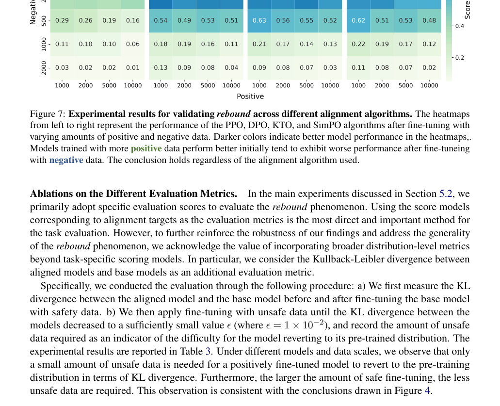
Figure 8: Reverse Fine-tuning Results on IMDb. Each subfigure from left to right shows the changes in LLMs with parameter sizes of 0.5B, 4B, and 7B, respectively. Models trained with more negative data initially perform worse, but perform better after fine-tuning with positive data. As the model size increases, the performance of the aligned model deteriorates more rapidly after fine-tuning with positive data.

图 8： IMDb 上的反向微调结果 。 从左到右各子图分别显示参数规模 0.5B、4B 与 7B 的 LLM 变化。用更多 负 数据训练的模型起初更差，用 正 数据微调后更好。随模型变大，对齐模型在用 正 数据微调后性能变化更快。

B.3 Additional Experiment of Internal Factor of Language Models’ Rebound

B.3 语言模型 反弹 内部因素的额外实验

Analysis of the Model Size Scale under Different Alignment Algorithms. To verify whether the rebound phenomenon in language models becomes more pronounced as model size increases persists across different alignment algorithms, we conduct experiments using the DPO algorithm. Specifically, we employ the Qwen1.5 model series as the base models and follow an experimental setup similar to that described in Section B.2. We carried out experiments on models with parameters 0.5B, 4B, and 7B. The experimental results, presented in Figure 9, demonstrate that rebound remains evident under the DPO algorithm, with its strength increasing as model size grows. This finding is consistent with the results reported in Figure 5 and further highlights the generality of elasticity in language models.

不同对齐算法下的模型规模分析。 为验证「语言模型 反弹 随模型规模增大而更明显」是否跨不同对齐算法成立，我们用 DPO 算法实验。具体以 Qwen1.5 系列为基座，实验设置类似附录 B.2。在 0.5B、4B 与 7B 参数模型上开展实验。图 9 表明：DPO 下 反弹 仍然明显，且随模型变大而增强。该发现与图 5 一致，并进一步凸显语言模型 弹性 的一般性。

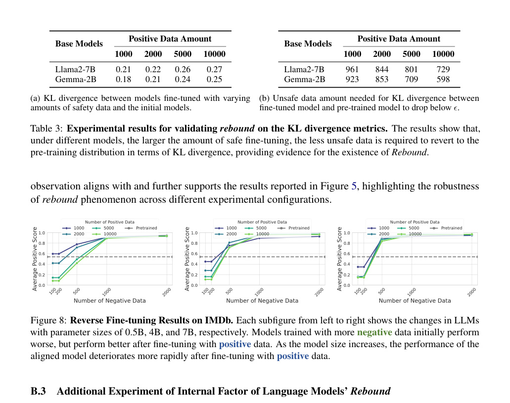
Figure 9: Experimental results for validating rebound increases with model size under DPO fine-tuning. Each subfigure from left to right shows the changes in LLMs with parameter sizes of 0.5B, 4B, and 7B. As the model size increases, the performance of the aligned model deteriorates more rapidly after fine-tuning with negative data.

图 9： 验证 DPO 微调下 反弹 随模型规模增大的实验结果 。 从左到右各子图分别显示参数规模 0.5B、4B 与 7B 的 LLM 变化。随模型变大，对齐模型在用 负 数据微调后性能下降更快。

Analysis of the Pre-training Data Volume. We present the experimental results for a broader range of pre-training data volumes in Figure 10. When the pre-training data volume is 0.1T, 0.5T, and 1.0T, the model still demonstrates the phenomenon that rebound increases with the volume of pre-training data, which is consistent with the results reported in Figure 6, where the pre-training data volumes range from 2.0T to 3.0T. Moreover, when comparing the experimental results in Figure 6 and Figure 10, we observe a consistent conclusion: as the pre-training data volume increases (from 0.5T to 3.0T), the rebound becomes more pronounced. Specifically, when the pre-training data volume increases, the initial performance decline caused by negative data fine-tuning occurs more rapidly, while the subsequent decline slows down. This indicates that larger pre-training data volumes amplify the rebound effect in language models.

预训练数据量分析。 图 10 给出更广预训练数据量范围的实验结果。当预训练数据量为 0.1T、0.5T 与 1.0T 时，模型仍展现 反弹 随预训练数据量增大而增强的现象，与图 6（预训练数据量 2.0T 至 3.0T）一致。此外，对比图 6 与图 10，我们得到一致结论：随预训练数据量从 0.5T 增至 3.0T， 反弹 更明显。具体地，预训练数据量增大时，负数据微调导致的初期性能下降更快，后续下降变缓。这表明更大预训练数据量放大了语言模型中的 反弹 效应。

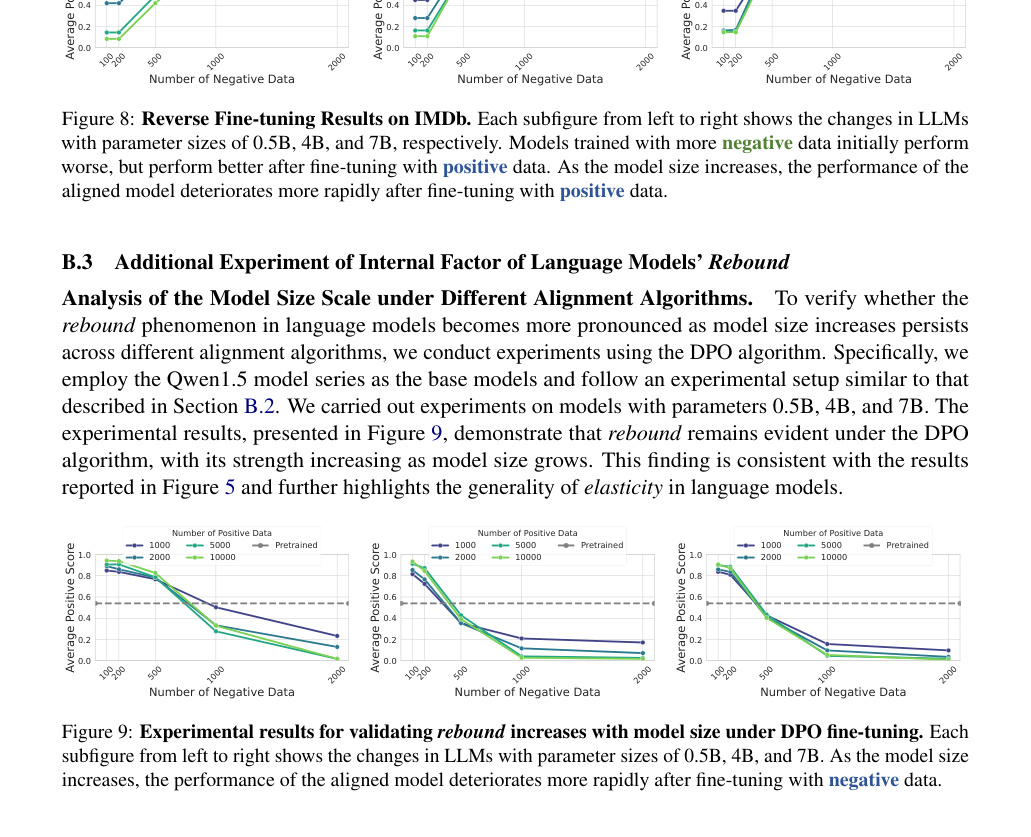
Figure 10: Experimental results for validating rebound increases with model pre-training data volume. Each subfigure from left to right shows the changes in pre-training data volumes of 0.1T, 0.5T, and 1.0T. As pre-training data volume increases, aligned model performance deteriorates more rapidly after fine-tuning with negative data.

图 10： 验证 反弹 随模型预训练数据量增大的实验结果 。 从左到右各子图分别显示预训练数据量 0.1T、0.5T 与 1.0T 的变化。随预训练数据量增加，对齐模型在用 负 数据微调后性能下降更快。

Appendix C Further Discussions of Language Models’ Elasticity

附录 C 关于语言模型 弹性 的进一步讨论

C.1 Transfer Learning and Language Models’ Elasticity

C.1 迁移学习与语言模型的 弹性

\mathcal{D}=\{\mathcal{X},P(X)\}

\mathcal{D}=\{\mathcal{X},P(X)\}

Specifically in the context of language models, transfer learning can almost encompass all models trained under the pre-training-finetuning paradigm. However, transfer learning does not capture the specific details of the model training process, nor does it explicitly incorporate the established theories that explain the varying degrees of difficulty in task transfer for LLMs. Therefore, while transfer learning provides a perspective to analyze various phenomena in LLMs from the standpoint of traditional machine learning, it does not offer concrete tools to explain these elasticity phenomena.

具体在语言模型语境下，迁移学习几乎可涵盖预训练-微调范式下训练的全部模型。但迁移学习未捕获模型训练过程的具体细节，也未显式纳入解释 LLM 任务迁移难度差异的既有理论。因此，虽提供从传统机器学习立场分析 LLM 诸现象的视角，却未给出解释这些 弹性 现象的具体工具。

Furthermore, in traditional transfer learning settings, positive and negative samples can only be considered as different partitions of the same dataset in classification tasks. However, in our case, these samples are used for autoregressive generation training, where the generation on positive samples and negative samples follows mutually conflicting input-output distributions. This is fundamentally different from classification tasks. Specifically for safe-unsafe generation, steering a language model’s generation from an unsafe input-output distribution to the opposite safe input-output distribution is a major challenge in generative language model research. This cannot be adequately explained by merely considering different partitions of the same data distribution.

此外，在传统迁移学习设定中，正负样本只能视为分类任务中同一数据集的不同划分。但在我们的情形中，这些样本用于自回归生成训练，正样本与负样本上的生成遵循相互冲突的输入-输出分布，与分类任务有本质不同。具体到安全-不安全生成，把语言模型生成从不安全输入-输出分布舵向相反的安全输入-输出分布，是生成式语言模型研究的主要挑战，不能仅靠把它们视为同一数据分布的不同划分来充分解释。

\theta_{1}

\theta_{1}

C.2 Discussions of Practical Steps to Mitigate Inverse Alignment Risks

C.2 缓解 逆向对齐 风险的实践步骤讨论

The emphasis on elasticity phenomenon in language model alignment highlights a crucial challenge for ensuring the safety and robustness of open-source models throughout their entire lifecycle. As our study demonstrates, the resistance of language models to alignment adjustments is fundamentally rooted in the substantial disparity in data volumes across different training phases. This insight suggests a practical mitigation strategy: customizing the scale of synthetic data through the elasticity mechanism offers a feasible pathway for the development of more robust alignment algorithms in the future.

强调语言模型对齐中的 弹性 现象，凸显了确保开源模型全生命周期安全与稳健的关键挑战。如本研究所示，语言模型对齐调整的阻力根本上根植于不同训练阶段数据量的巨大差距。这一洞见提示一条实践缓解策略：通过弹性机制定制合成数据规模，为未来开发更稳健对齐算法提供可行路径。

• We discover that the resistance of language models to alignment is essentially due to the significant differences in data volume across various training processes. Therefore, a straightforward idea is to ensure that the training data volumes corresponding to different alignment targets are as similar as possible during the alignment process. This approach helps avoid resistance effects on alignment targets with smaller training data volumes due to subsequent perturbations.

• 我们发现语言模型对齐阻力本质上源于各训练过程数据量的显著差异。因此一个直接想法是：在对齐过程中尽量使不同对齐目标对应的训练数据量相近。这有助于避免因后续扰动而对训练数据量较小的对齐目标产生阻力效应。

• The elasticity theorem provides a feasible method for customizing data ratios, thereby quantitatively measuring the amount of various types of data needed for a model to meet expected goals. Specifically, for an aligned language model, during subsequent alignment processes, the elasticity theorem indicates that there is an inherent loss of elasticity dependent on data volume ratios when learning unrelated distributions. Therefore, to ensure that previously aligned targets remain satisfied during subsequent alignment, the training objective can be transformed into a constrained optimization problem to quantitatively calculate the data volume required for new target alignment.

• 弹性定理提供了定制数据比例的可行方法，从而可定量度量模型达到预期目标所需的各类数据量。具体地，对已对齐语言模型，在后续对齐过程中，弹性定理表明：学习无关分布时存在依赖数据量比例的固有弹性损失。因此，为确保先前对齐目标在后续对齐中仍被满足，可将训练目标转化为约束优化问题，定量计算新目标对齐所需数据量。

• The current challenge in implementing algorithms based on the elasticity theory, mainly lies in the lack of a sufficient theoretical foundation to characterize the specific features of current datasets. This makes it difficult to distinguish the independent and differently distributed premises of different datasets in the elasticity theory. Since real-world datasets often contain fused features, a possible future research direction is to finely characterize the features of datasets with fused characteristics.

• 当前实现基于弹性理论的算法的主要挑战，在于缺乏充分理论基础来刻画当前数据集的具体特征。这使得难以区分弹性理论中不同数据集的独立不同分布前提。由于真实世界数据集常含融合特征，一个可能的未来研究方向是精细刻画具有融合特征的数据集特征。

C.3 Discussions of Quantitatively Characterize the Impact of Dataset Size on Elasticity

C.3 定量刻画数据集大小对 弹性 影响的讨论

Considering that, as indicated in Theorem 4.2, the difference in dataset size is a key factor contributing to the elasticity phenomenon, quantitatively characterizing the impact of dataset size on elasticity is indeed crucial for both theoretical understanding and practical alignment design. In this section, we present preliminary explorations, based on experimental observations, on quantifying the influence of dataset size on elasticity, as well as the current limitations in achieving this goal.

考虑到如定理 4.2 所示，数据集大小差异是促成 弹性 现象的关键因素，定量刻画数据集大小对 弹性 的影响对理论理解与实践对齐设计确实至关重要。本节基于实验观察，对量化数据集大小对弹性的影响以及达成该目标的当前局限，给出初步探索。

By synthesizing observations from Figure 6 in the main text and Figure 10 in the appendix, we find that for the tinyllama series models, when the pre-training data volume is merely 0.1T, there is almost no significant resistance phenomenon observed; the positive level of the model’s output does not change significantly with an increase in negative data. However, when the pre-training data volume reaches 0.5T, the resistance phenomenon of the language model becomes notably observable. Considering the continuity between pre-training data and model resistance, this suggests that the significant change point of the resistance phenomenon should lie between 0.1T and 0.5T.

综合正文图 6 与附录图 10 的观察，我们发现：对 tinyllama 系列模型，当预训练数据量仅 0.1T 时，几乎观察不到显著阻力现象；模型输出的正向水平随负数据增加并无明显变化。但当预训练数据量达到 0.5T 时，语言模型的阻力现象变得显著可观察。考虑到预训练数据与模型阻力之间的连续性，这表明阻力现象的显著变化点应位于 0.1T 与 0.5T 之间。

Regrettably, there are still challenges in training a series of models with continuously varying pre-training data volumes, and we currently lack sufficiently fine-grained training data samples to conduct such precise series model training. This limitation prevents us from accurately determining the critical point where the resistance phenomenon becomes significant. Therefore, although we can suggest a possible range, accurately quantifying this threshold in practice remains a considerable challenge. We hope that future research will further address this issue by developing more controllable model series and fine-grained pre-training datasets to enable a clearer, quantitative characterization of elasticity .

遗憾的是，训练预训练数据量连续变化的一系列模型仍有挑战，我们目前也缺乏足够细粒度的训练数据样本来开展如此精确的系列模型训练。该局限使我们无法准确确定阻力现象变得显著的临界点。因此，虽可给出可能区间，在实践中准确量化该阈值仍是相当大的挑战。

Language Models Resist Alignment: Evidence From Data Compression

Language Models Resist Alignment：来自数据压缩的证据

Abstract

摘要

1 Introduction

1 引言

2 Related Work

2 相关工作

The Fragility of LLMs Alignment

LLM 对齐的脆弱性

3 What is Elasticity?

3 什么是弹性？

3.1 Preliminaries

3.1 预备知识

Pre-training.

预训练。

Supervised Fine-tuning (SFT).

监督微调（SFT）。

Lossless Compression.

无损压缩。

Compression and Prediction.

压缩与预测。

3.2 The Compression Protocol of LLMs

3.2 LLM 的压缩协议

Definition 3.1(Token Tree T\mathcal{T}T).

定义 3.1（Token 树 T\mathcal{T}T）。

Assumption 3.2(Scale of T\mathcal{T}T is Monotone with Model Size).

假设 3.2（T\mathcal{T}T 的规模随模型大小单调）。

Definition 3.3(The Compression Protocal).

定义 3.3（压缩协议）。

Theorem 3.4(Ideal Code Length).

Theorem 3.4(Ideal Code Length).

3.3 The Formal Definition of Elasticity

3.3 弹性的形式定义

Definition 3.6(The Elasticity of LLMs).

Definition 3.6(The Elasticity of LLMs).

4 Why Elasticity Affects Alignment?

4 为什么弹性影响对齐？

4.1 Formal Derivation of Elasticity

4.1 弹性的形式推导

Definition 4.1(Normalized Compression Rate).

定义 4.1（归一化压缩率）。

Theorem 4.2(Elasticity of Language Models).

Theorem 4.2(Elasticity of Language Models).

4.2 Elasticity and Inverse Alignment

4.2 弹性与逆向对齐

4.3 Elasticity and the Hooke’s Law.

4.3 弹性与胡克定律

5 How Elasticity Resists Alignment?

5 弹性如何抵制对齐？

5.1 Existence of Language Models’ Resistance

5.1 语言模型阻力的存在性

Experiment Design.

实验设计。

Experiment Setup.

实验设置。

Experiment Results.

实验结果。

5.2 Existence of Rebound

5.2 反弹的存在性

Experiment Design.

实验设计。

Tasks and Datasets.

任务与数据集。

Evaluation and Metrics.

评测与指标。

Experiment Results.

实验结果。

5.3 Internal Factor of Rebound

5.3 反弹的内部因素

Rebound Increases with Model Size.

反弹随模型规模增大。

Rebound Increases with Pre-training Data Volume.

反弹随预训练数据量增大。

6 Conclusion and Outlook

6 结论与展望

6.1 Limitations

6.1 局限

6.2 Broader Impacts

6.2 更广泛影响

Definition 3.1(Token Tree $\mathcal{T}$ ).

定义 3.1（Token 树 $\mathcal{T}$ ）。

Assumption 3.2(Scale of $\mathcal{T}$ is Monotone with Model Size).

假设 3.2（ $\mathcal{T}$ 的规模随模型大小单调）。

References

参考文献
Achiam et al. (2023) Josh Achiam, Steven Adler, Sandhini Agarwal, Lama Ahmad, Ilge Akkaya, Florencia Leoni Aleman, Diogo Almeida, Janko Altenschmidt, Sam Altman, Shyamal Anadkat, et al. 2023. Gpt-4 technical report. arXiv preprint arXiv:2303.08774 .
Anwar et al. (2024) Usman Anwar, Abulhair Saparov, Javier Rando, Daniel Paleka, Miles Turpin, Peter Hase, Ekdeep Singh Lubana, Erik Jenner, Stephen Casper, Oliver Sourbut, et al. 2024. Foundational challenges in assuring alignment and safety of large language models. arXiv preprint arXiv:2404.09932 .
Askell et al. (2021) Amanda Askell, Yuntao Bai, Anna Chen, Dawn Drain, Deep Ganguli, Tom Henighan, Andy Jones, Nicholas Joseph, Ben Mann, Nova DasSarma, et al. 2021. A general language assistant as a laboratory for alignment. arXiv preprint arXiv:2112.00861 .
Bai et al. (2023) Jinze Bai, Shuai Bai, Yunfei Chu, Zeyu Cui, Kai Dang, Xiaodong Deng, Yang Fan, Wenbin Ge, Yu Han, Fei Huang, et al. 2023. Qwen technical report. arXiv preprint arXiv:2309.16609 .
Bai et al. (2022a) Yuntao Bai, Andy Jones, Kamal Ndousse, Amanda Askell, Anna Chen, Nova DasSarma, Dawn Drain, Stanislav Fort, Deep Ganguli, Tom Henighan, et al. 2022a. Training a helpful and harmless assistant with reinforcement learning from human feedback. arXiv preprint arXiv:2204.05862 .
Bai et al. (2022b) Yuntao Bai, Saurav Kadavath, Sandipan Kundu, Amanda Askell, Jackson Kernion, Andy Jones, Anna Chen, Anna Goldie, Azalia Mirhoseini, Cameron McKinnon, et al. 2022b. Constitutional ai: Harmlessness from ai feedback. arXiv preprint arXiv:2212.08073 .
Baker et al. (2025) Bowen Baker, Joost Huizinga, Leo Gao, Zehao Dou, Melody Y Guan, Aleksander Madry, Wojciech Zaremba, Jakub Pachocki, and David Farhi. 2025. Monitoring reasoning models for misbehavior and the risks of promoting obfuscation. arXiv preprint arXiv:2503.11926 .
Bengio et al. (2025) Yoshua Bengio, Sören Mindermann, Daniel Privitera, Tamay Besiroglu, Rishi Bommasani, Stephen Casper, Yejin Choi, Philip Fox, Ben Garfinkel, Danielle Goldfarb, et al. 2025. International ai safety report. arXiv preprint arXiv:2501.17805 .
Casper et al. (2023) Stephen Casper, Xander Davies, Claudia Shi, Thomas Krendl Gilbert, Jérémy Scheurer, Javier Rando, Rachel Freedman, Tomasz Korbak, David Lindner, Pedro Freire, Tony Tong Wang, Samuel Marks, Charbel-Raphael Segerie, Micah Carroll, Andi Peng, Phillip Christoffersen, Mehul Damani, Stewart Slocum, Usman Anwar, Anand Siththaranjan, Max Nadeau, Eric J Michaud, Jacob Pfau, Dmitrii Krasheninnikov, Xin Chen, Lauro Langosco, Peter Hase, Erdem Biyik, Anca Dragan, David Krueger, Dorsa Sadigh, and Dylan Hadfield-Menell. 2023. Open problems and fundamental limitations of reinforcement learning from human feedback. Transactions on Machine Learning Research . Survey Certification.
Chen et al. (2024) Yingfa Chen, Zhengyan Zhang, Xu Han, Chaojun Xiao, Zhiyuan Liu, Chen Chen, Kuai Li, Tao Yang, and Maosong Sun. 2024. Robust and scalable model editing for large language models. arXiv preprint arXiv:2403.17431 .
Cohen et al. (2024) Michael K Cohen, Marcus Hutter, Yoshua Bengio, and Stuart Russell. 2024. Rl, but don’t do anything i wouldn’t do. arXiv preprint arXiv:2410.06213 .
Cui et al. (2024) Ganqu Cui, Lifan Yuan, Ning Ding, Guanming Yao, Bingxiang He, Wei Zhu, Yuan Ni, Guotong Xie, Ruobing Xie, Yankai Lin, et al. 2024. Ultrafeedback: Boosting language models with scaled ai feedback. In Forty-first International Conference on Machine Learning .
Dai et al. (2024) Josef Dai, Xuehai Pan, Ruiyang Sun, Jiaming Ji, Xinbo Xu, Mickel Liu, Yizhou Wang, and Yaodong Yang. 2024. Safe rlhf: Safe reinforcement learning from human feedback. In The Twelfth International Conference on Learning Representations .
Delétang et al. (2023) Grégoire Delétang, Anian Ruoss, Paul-Ambroise Duquenne, Elliot Catt, Tim Genewein, Christopher Mattern, Jordi Grau-Moya, Li Kevin Wenliang, Matthew Aitchison, Laurent Orseau, et al. 2023. Language modeling is compression. arXiv preprint arXiv:2309.10668 .
Dong et al. (2023) Hanze Dong, Wei Xiong, Deepanshu Goyal, Yihan Zhang, Winnie Chow, Rui Pan, Shizhe Diao, Jipeng Zhang, SHUM KaShun, and Tong Zhang. 2023. Raft: Reward ranked finetuning for generative foundation model alignment. Transactions on Machine Learning Research .
Dong et al. (2024) Zhichen Dong, Zhanhui Zhou, Chao Yang, Jing Shao, and Yu Qiao. 2024. Attacks, defenses and evaluations for llm conversation safety: A survey. arXiv preprint arXiv:2402.09283 .
Eiras et al. (2024) Francisco Eiras, Aleksandar Petrov, Bertie Vidgen, Christian Schroeder De Witt, Fabio Pizzati, Katherine Elkins, Supratik Mukhopadhyay, Adel Bibi, Botos Csaba, Fabro Steibel, et al. 2024. Near to mid-term risks and opportunities of open-source generative ai. arXiv preprint arXiv:2404.17047 .
Ethayarajh et al. (2024) Kawin Ethayarajh, Winnie Xu, Niklas Muennighoff, Dan Jurafsky, and Douwe Kiela. 2024. Kto: Model alignment as prospect theoretic optimization. arXiv preprint arXiv:2402.01306 .
Garfinkel and Dafoe (2021) Ben Garfinkel and Allan Dafoe. 2021. How does the offense-defense balance scale? In Emerging Technologies and International Stability , pages 247–274. Routledge.
Goldstein et al. (2023) Josh A Goldstein, Girish Sastry, Micah Musser, Renee DiResta, Matthew Gentzel, and Katerina Sedova. 2023. Generative language models and automated influence operations: Emerging threats and potential mitigations. arXiv preprint arXiv:2301.04246 .
Greenblatt et al. (2024) Ryan Greenblatt, Carson Denison, Benjamin Wright, Fabien Roger, Monte MacDiarmid, Sam Marks, Johannes Treutlein, Tim Belonax, Jack Chen, David Duvenaud, et al. 2024. Alignment faking in large language models. arXiv preprint arXiv:2412.14093 .
Gulcehre et al. (2023) Caglar Gulcehre, Tom Le Paine, Srivatsan Srinivasan, Ksenia Konyushkova, Lotte Weerts, Abhishek Sharma, Aditya Siddhant, Alex Ahern, Miaosen Wang, Chenjie Gu, et al. 2023. Reinforced self-training (rest) for language modeling. arXiv preprint arXiv:2308.08998 .
Hartmann et al. (2023) Jochen Hartmann, Mark Heitmann, Christian Siebert, and Christina Schamp. 2023. More than a feeling: Accuracy and application of sentiment analysis. International Journal of Research in Marketing , 40(1):75–87.
He et al. (2024) Luxi He, Mengzhou Xia, and Peter Henderson. 2024. What’s in your" safe" data?: Identifying benign data that breaks safety. arXiv preprint arXiv:2404.01099 .
Hooke (2016) Robert Hooke. 2016. Lectures de potentia restitutiva, or of spring explaining the power of springing bodies . 6. John Martyn.
Huang et al. (2024) Yuzhen Huang, Jinghan Zhang, Zifei Shan, and Junxian He. 2024. Compression represents intelligence linearly. arXiv preprint arXiv:2404.09937 .
Hubinger et al. (2024) Evan Hubinger, Carson Denison, Jesse Mu, Mike Lambert, Meg Tong, Monte MacDiarmid, Tamera Lanham, Daniel M Ziegler, Tim Maxwell, Newton Cheng, et al. 2024. Sleeper agents: Training deceptive llms that persist through safety training. arXiv preprint arXiv:2401.05566 .
Huffman (1952) David A Huffman. 1952. A method for the construction of minimum-redundancy codes. Proceedings of the IRE , 40(9):1098–1101.
Huh et al. (2024) Minyoung Huh, Brian Cheung, Tongzhou Wang, and Phillip Isola. 2024. Position: The platonic representation hypothesis. In Forty-first International Conference on Machine Learning .
Hutter (2005) Marcus Hutter. 2005. Universal Artificial Intelligence: Sequential Decisions Based On Algorithmic Probability . Springer Science & Business Media.
IDAIS-Beijing (2024) IDAIS-Beijing. 2024. Consensus statement on red lines in artificial intelligence .
Jain et al. (2023) Samyak Jain, Robert Kirk, Ekdeep Singh Lubana, Robert P Dick, Hidenori Tanaka, Edward Grefenstette, Tim Rocktäschel, and David Scott Krueger. 2023. Mechanistically analyzing the effects of fine-tuning on procedurally defined tasks. arXiv preprint arXiv:2311.12786 .
Jervis (1978) Robert Jervis. 1978. Cooperation under the security dilemma. World politics , 30(2):167–214.
Ji et al. (2024a) Jiaming Ji, Boyuan Chen, Hantao Lou, Donghai Hong, Borong Zhang, Xuehai Pan, Juntao Dai, and Yaodong Yang. 2024a. Aligner: Achieving efficient alignment through weak-to-strong correction. arXiv preprint arXiv:2402.02416 .
Ji et al. (2024b) Jiaming Ji, Donghai Hong, Borong Zhang, Boyuan Chen, Josef Dai, Boren Zheng, Tianyi Qiu, Boxun Li, and Yaodong Yang. 2024b. Pku-saferlhf: Towards multi-level safety alignment for llms with human preference. arXiv preprint arXiv:2406.15513 .
Ji et al. (2024c) Jiaming Ji, Mickel Liu, Josef Dai, Xuehai Pan, Chi Zhang, Ce Bian, Boyuan Chen, Ruiyang Sun, Yizhou Wang, and Yaodong Yang. 2024c. Beavertails: Towards improved safety alignment of llm via a human-preference dataset. Advances in Neural Information Processing Systems , 36.
Ji et al. (2023) Jiaming Ji, Tianyi Qiu, Boyuan Chen, Borong Zhang, Hantao Lou, Kaile Wang, Yawen Duan, Zhonghao He, Jiayi Zhou, Zhaowei Zhang, et al. 2023. Ai alignment: A comprehensive survey. arXiv preprint arXiv:2310.19852 .
Ji et al. (2024d) Jiaming Ji, Jiayi Zhou, Hantao Lou, Boyuan Chen, Donghai Hong, Xuyao Wang, Wenqi Chen, Kaile Wang, Rui Pan, Jiahao Li, et al. 2024d. Align anything: Training all-modality models to follow instructions with language feedback. arXiv preprint arXiv:2412.15838 .
Kaplan et al. (2020) Jared Kaplan, Sam McCandlish, Tom Henighan, Tom B Brown, Benjamin Chess, Rewon Child, Scott Gray, Alec Radford, Jeffrey Wu, and Dario Amodei. 2020. Scaling laws for neural language models. arXiv preprint arXiv:2001.08361 .
Kukreja et al. (2024) Sanjay Kukreja, Tarun Kumar, Amit Purohit, Abhijit Dasgupta, and Debashis Guha. 2024. A literature survey on open source large language models. In Proceedings of the 2024 7th International Conference on Computers in Management and Business , pages 133–143.
Lang et al. (2024) Leon Lang, Davis Foote, Stuart J Russell, Anca Dragan, Erik Jenner, and Scott Emmons. 2024. When your ais deceive you: Challenges of partial observability in reinforcement learning from human feedback. Advances in Neural Information Processing Systems , 37:93240–93299.
Lee et al. (2023) Harrison Lee, Samrat Phatale, Hassan Mansoor, Kellie Lu, Thomas Mesnard, Colton Bishop, Victor Carbune, and Abhinav Rastogi. 2023. Rlaif: Scaling reinforcement learning from human feedback with ai feedback. arXiv preprint arXiv:2309.00267 .
Li et al. (2025) Bohan Li, Longxu Dou, Yutai Hou, Yunlong Feng, Honglin Mu, Enbo Wang, Qingfu Zhu, Qinghua Sun, and Wanxiang Che. 2025. Mixpro: Simple yet effective data augmentation for prompt-based learning. International Journal of Machine Learning and Cybernetics , pages 1–20.
Li et al. (2023) Ziniu Li, Tian Xu, Yushun Zhang, Yang Yu, Ruoyu Sun, and Zhi-Quan Luo. 2023. Remax: A simple, effective, and efficient method for aligning large language models. arXiv preprint arXiv:2310.10505 .
Lin et al. (2025) Lizhi Lin, Honglin Mu, Zenan Zhai, Minghan Wang, Yuxia Wang, Renxi Wang, Junjie Gao, Yixuan Zhang, Wanxiang Che, Timothy Baldwin, et al. 2025. Against the achilles’ heel: A survey on red teaming for generative models. Journal of Artificial Intelligence Research , 82:687–775.
Lin et al. (2022) Stephanie Lin, Jacob Hilton, and Owain Evans. 2022. Truthfulqa: Measuring how models mimic human falsehoods. In Proceedings of the 60th Annual Meeting of the Association for Computational Linguistics (Volume 1: Long Papers) , pages 3214–3252.
Liu et al. (2024) Tianqi Liu, Wei Xiong, Jie Ren, Lichang Chen, Junru Wu, Rishabh Joshi, Yang Gao, Jiaming Shen, Zhen Qin, Tianhe Yu, et al. 2024. Rrm: Robust reward model training mitigates reward hacking. arXiv preprint arXiv:2409.13156 .
Maas et al. (2011) Andrew Maas, Raymond E Daly, Peter T Pham, Dan Huang, Andrew Y Ng, and Christopher Potts. 2011. Learning word vectors for sentiment analysis. In Proceedings of the 49th annual meeting of the association for computational linguistics: Human language technologies , pages 142–150.
Madiega (2021) Tambiama Madiega. 2021. Artificial intelligence act. European Parliament: European Parliamentary Research Service .
Marks et al. (2025) Samuel Marks, Johannes Treutlein, Trenton Bricken, Jack Lindsey, Jonathan Marcus, Siddharth Mishra-Sharma, Daniel Ziegler, Emmanuel Ameisen, Joshua Batson, Tim Belonax, et al. 2025. Auditing language models for hidden objectives. arXiv preprint arXiv:2503.10965 .
Meng et al. (2024) Yu Meng, Mengzhou Xia, and Danqi Chen. 2024. Simpo: Simple preference optimization with a reference-free reward. Advances in Neural Information Processing Systems , 37:124198–124235.
Mingard et al. (2021) Chris Mingard, Guillermo Valle-Pérez, Joar Skalse, and Ard A Louis. 2021. Is sgd a bayesian sampler? well, almost. Journal of Machine Learning Research , 22(79):1–64.
Mökander et al. (2024) Jakob Mökander, Jonas Schuett, Hannah Rose Kirk, and Luciano Floridi. 2024. Auditing large language models: a three-layered approach. AI and Ethics , 4(4):1085–1115.
Murphy (2023) Kevin P Murphy. 2023. Probabilistic machine learning: Advanced topics . MIT press.
Newman (2005) Mark EJ Newman. 2005. Power laws, pareto distributions and zipf’s law. Contemporary physics , 46(5):323–351.
Ouyang et al. (2022) Long Ouyang, Jeffrey Wu, Xu Jiang, Diogo Almeida, Carroll Wainwright, Pamela Mishkin, Chong Zhang, Sandhini Agarwal, Katarina Slama, Alex Ray, et al. 2022. Training language models to follow instructions with human feedback. Advances in neural information processing systems , 35:27730–27744.
Park et al. (2024) Peter S Park, Simon Goldstein, Aidan O’Gara, Michael Chen, and Dan Hendrycks. 2024. Ai deception: A survey of examples, risks, and potential solutions. Patterns , 5(5).
Qi et al. (2024a) Xiangyu Qi, Ashwinee Panda, Kaifeng Lyu, Xiao Ma, Subhrajit Roy, Ahmad Beirami, Prateek Mittal, and Peter Henderson. 2024a. Safety alignment should be made more than just a few tokens deep. arXiv preprint arXiv:2406.05946 .
Qi et al. (2024b) Xiangyu Qi, Yi Zeng, Tinghao Xie, Pin-Yu Chen, Ruoxi Jia, Prateek Mittal, and Peter Henderson. 2024b. Fine-tuning aligned language models compromises safety, even when users do not intend to! In The Twelfth International Conference on Learning Representations .
Qian et al. (2024) Chen Qian, Jie Zhang, Wei Yao, Dongrui Liu, Zhenfei Yin, Yu Qiao, Yong Liu, and Jing Shao. 2024. Towards tracing trustworthiness dynamics: Revisiting pre-training period of large language models. arXiv preprint arXiv:2402.19465 .
Rafailov et al. (2024) Rafael Rafailov, Archit Sharma, Eric Mitchell, Christopher D Manning, Stefano Ermon, and Chelsea Finn. 2024. Direct preference optimization: Your language model is secretly a reward model. Advances in Neural Information Processing Systems , 36.
Reuel et al. (2024) Anka Reuel, Ben Bucknall, Stephen Casper, Tim Fist, Lisa Soder, Onni Aarne, Lewis Hammond, Lujain Ibrahim, Alan Chan, Peter Wills, et al. 2024. Open problems in technical ai governance. arXiv preprint arXiv:2407.14981 .
Revel et al. (2024) Manon Revel, Matteo Cargnelutti, Tyna Eloundou, and Greg Leppert. 2024. Seal: Systematic error analysis for value alignment. arXiv preprint arXiv:2408.10270 .
Sandbrink (2023) Jonas B Sandbrink. 2023. Artificial intelligence and biological misuse: Differentiating risks of language models and biological design tools. arXiv preprint arXiv:2306.13952 .
Seger et al. (2023) Elizabeth Seger, Noemi Dreksler, Richard Moulange, Emily Dardaman, Jonas Schuett, K Wei, Christoph Winter, Mackenzie Arnold, Seán Ó hÉigeartaigh, Anton Korinek, et al. 2023. Open-sourcing highly capable foundation models: An evaluation of risks, benefits, and alternative methods for pursuing open-source objectives. arXiv preprint arXiv:2311.09227 .
Shannon (1948) Claude Elwood Shannon. 1948. A mathematical theory of communication. The Bell system technical journal , 27(3):379–423.
Shapiro and Siegel (2010) Jacob N Shapiro and David A Siegel. 2010. Is this paper dangerous? balancing secrecy and openness in counterterrorism. Security Studies , 19(1):66–98.
Sheshadri et al. (2024) Abhay Sheshadri, Aidan Ewart, Phillip Guo, Aengus Lynch, Cindy Wu, Vivek Hebbar, Henry Sleight, Asa Cooper Stickland, Ethan Perez, Dylan Hadfield-Menell, et al. 2024. Targeted latent adversarial training improves robustness to persistent harmful behaviors in llms. arXiv e-prints , pages arXiv–2407.
Taori et al. (2023) Rohan Taori, Ishaan Gulrajani, Tianyi Zhang, Yann Dubois, Xuechen Li, Carlos Guestrin, Percy Liang, and Tatsunori B Hashimoto. 2023. Stanford alpaca: An instruction-following llama model. https://github.com/tatsu-lab/stanford_alpaca .
Team et al. (2024) Gemma Team, Thomas Mesnard, Cassidy Hardin, Robert Dadashi, Surya Bhupatiraju, Shreya Pathak, Laurent Sifre, Morgane Rivière, Mihir Sanjay Kale, Juliette Love, et al. 2024. Gemma: Open models based on gemini research and technology. arXiv preprint arXiv:2403.08295 .
Touvron et al. (2023) Hugo Touvron, Louis Martin, Kevin Stone, Peter Albert, Amjad Almahairi, Yasmine Babaei, Nikolay Bashlykov, Soumya Batra, Prajjwal Bhargava, Shruti Bhosale, et al. 2023. Llama 2: Open foundation and fine-tuned chat models. arXiv preprint arXiv:2307.09288 .
Urbina et al. (2022) Fabio Urbina, Filippa Lentzos, Cédric Invernizzi, and Sean Ekins. 2022. Dual use of artificial-intelligence-powered drug discovery. Nature machine intelligence , 4(3):189–191.
Wei et al. (2024) Boyi Wei, Kaixuan Huang, Yangsibo Huang, Tinghao Xie, Xiangyu Qi, Mengzhou Xia, Prateek Mittal, Mengdi Wang, and Peter Henderson. 2024. Assessing the brittleness of safety alignment via pruning and low-rank modifications. arXiv preprint arXiv:2402.05162 .
Weiss et al. (2016) Karl Weiss, Taghi M Khoshgoftaar, and DingDing Wang. 2016. A survey of transfer learning. Journal of Big data , 3:1–40.
Wen et al. (2024) Jiaxin Wen, Ruiqi Zhong, Akbir Khan, Ethan Perez, Jacob Steinhardt, Minlie Huang, Samuel R Bowman, He He, and Shi Feng. 2024. Language models learn to mislead humans via rlhf. arXiv preprint arXiv:2409.12822 .
Witten et al. (1987) Ian H Witten, Radford M Neal, and John G Cleary. 1987. Arithmetic coding for data compression. Communications of the ACM , 30(6):520–540.
Xiao et al. (2024) Chaojun Xiao, Jie Cai, Weilin Zhao, Guoyang Zeng, Biyuan Lin, Jie Zhou, Zhi Zheng, Xu Han, Zhiyuan Liu, and Maosong Sun. 2024. Densing law of llms. arXiv preprint arXiv:2412.04315 .
Xiong et al. (2024) Wei Xiong, Hanze Dong, Chenlu Ye, Ziqi Wang, Han Zhong, Heng Ji, Nan Jiang, and Tong Zhang. 2024. Iterative preference learning from human feedback: Bridging theory and practice for rlhf under kl-constraint. In Forty-first International Conference on Machine Learning .
Yang et al. (2023a) Kevin Yang, Dan Klein, Asli Celikyilmaz, Nanyun Peng, and Yuandong Tian. 2023a. Rlcd: Reinforcement learning from contrastive distillation for language model alignment. arXiv preprint arXiv:2307.12950 .
Yang et al. (2023b) Xianjun Yang, Xiao Wang, Qi Zhang, Linda Petzold, William Yang Wang, Xun Zhao, and Dahua Lin. 2023b. Shadow alignment: The ease of subverting safely-aligned language models. arXiv preprint arXiv:2310.02949 .
Yang et al. (2024) Yuqing Yang, Ethan Chern, Xipeng Qiu, Graham Neubig, and Pengfei Liu. 2024. Alignment for honesty. Advances in Neural Information Processing Systems , 37:63565–63598.
Zhang et al. (2024a) Peiyuan Zhang, Guangtao Zeng, Tianduo Wang, and Wei Lu. 2024a. Tinyllama: An open-source small language model. arXiv preprint arXiv:2401.02385 .
Zhang et al. (2025) Xuanliang Zhang, Dingzirui Wang, Longxu Dou, Qingfu Zhu, and Wanxiang Che. 2025. A survey of table reasoning with large language models. Frontiers of Computer Science , 19(9):199348.
Zhang et al. (2024b) Zhexin Zhang, Junxiao Yang, Pei Ke, Shiyao Cui, Chujie Zheng, Hongning Wang, and Minlie Huang. 2024b. Safe unlearning: A surprisingly effective and generalizable solution to defend against jailbreak attacks. arXiv preprint arXiv:2407.02855 .
Zhou et al. (2024) Chunting Zhou, Pengfei Liu, Puxin Xu, Srinivasan Iyer, Jiao Sun, Yuning Mao, Xuezhe Ma, Avia Efrat, Ping Yu, Lili Yu, et al. 2024. Lima: Less is more for alignment. Advances in Neural Information Processing Systems , 36.
Zhou et al. (2025) Jiayi Zhou, Jiaming Ji, Josef Dai, and Yaodong Yang. 2025. Sequence to sequence reward modeling: Improving rlhf by language feedback. In Proceedings of the AAAI Conference on Artificial Intelligence , volume 39, pages 27765–27773.
Zhou et al. (2023) Zhanhui Zhou, Jie Liu, Jing Shao, Xiangyu Yue, Chao Yang, Wanli Ouyang, and Yu Qiao. 2023. Beyond one-preference-fits-all alignment: Multi-objective direct preference optimization. arXiv preprint arXiv:2310.03708 .
Zhuang et al. (2020) Fuzhen Zhuang, Zhiyuan Qi, Keyu Duan, Dongbo Xi, Yongchun Zhu, Hengshu Zhu, Hui Xiong, and Qing He. 2020. A comprehensive survey on transfer learning. Proceedings of the IEEE , 109(1):43–76.
Zipf (1946) George Kingsley Zipf. 1946. The psychology of language. In Encyclopedia of psychology , pages 332–341. Philosophical Library.
Zou et al. (2023) Andy Zou, Zifan Wang, J Zico Kolter, and Matt Fredrikson. 2023. Universal and transferable adversarial attacks on aligned language models. arXiv preprint arXiv:2307.15043 .