Junction Tree Variational Autoencoder for Molecular Graph Generation
Junction Tree Variational Autoencoder for Molecular Graph Generation
用于分子图生成的连接树变分自编码器
Wengong Jin Affiliation: MIT Computer Science & Artificial Intelligence Lab Correspondence to: wengong@csail.mit.edu Regina Barzilay Affiliation: MIT Computer Science & Artificial Intelligence Lab Tommi Jaakkola Affiliation: MIT Computer Science & Artificial Intelligence Lab
Supplementary Material
补充材料
Wengong Jin Affiliation: MIT Computer Science & Artificial Intelligence Lab Correspondence to: wengong@csail.mit.edu Regina Barzilay Affiliation: MIT Computer Science & Artificial Intelligence Lab Tommi Jaakkola Affiliation: MIT Computer Science & Artificial Intelligence Lab
Abstract
摘要
We seek to automate the design of molecules based on specific chemical properties. In computational terms, this task involves continuous embedding and generation of molecular graphs. Our primary contribution is the direct realization of molecular graphs, a task previously approached by generating linear SMILES strings instead of graphs. Our junction tree variational autoencoder generates molecular graphs in two phases, by first generating a tree-structured scaffold over chemical substructures, and then combining them into a molecule with a graph message passing network. This approach allows us to incrementally expand molecules while maintaining chemical validity at every step. We evaluate our model on multiple tasks ranging from molecular generation to optimization. Across these tasks, our model outperforms previous state-of-the-art baselines by a significant margin.
我们希望根据特定化学性质自动设计分子。从计算角度看,这一任务涉及分子图的连续嵌入与生成。我们的主要贡献是直接实现分子图——此前的做法是生成线性的 SMILES 字符串,而不是图。我们的连接树变分自编码器分两阶段生成分子图:先在化学子结构上生成树状骨架,再用图消息传递网络把它们组合成分子。这种方法可以逐步扩展分子,并在每一步保持化学有效性。我们在从分子生成到优化的多项任务上评估模型。在这些任务上,我们的模型以明显优势超过此前的最优基线。
1 Introduction
1 引言
Keywords:
The key challenge of drug discovery is to find target molecules with desired chemical properties. Currently, this task takes years of development and exploration by expert chemists and pharmacologists. Our ultimate goal is to automate this process. From a computational perspective, we decompose the challenge into two complementary subtasks: learning to represent molecules in a continuous manner that facilitates the prediction and optimization of their properties (encoding); and learning to map an optimized continuous representation back into a molecular graph with improved properties (decoding). While deep learning has been extensively investigated for molecular graph encoding (Duvenaud et al. 2015; Kearnes et al. 2016; Gilmer et al. 2017), the harder combinatorial task of molecular graph generation from latent representation remains under-explored.
关键词:
药物发现的关键挑战,是找到具有所需化学性质的目标分子。目前,这项工作需要化学家和药理学家花费数年去开发和探索。我们的最终目标是把这一过程自动化。从计算角度,我们把挑战拆成两个互补的子任务:学习以连续方式表示分子,以便预测和优化其性质(编码);以及学习把优化后的连续表示映射回性质更好的分子图(解码)。尽管深度学习已被广泛用于分子图编码(Duvenaud 等,2015;Kearnes 等,2016;Gilmer 等,2017),从潜表示生成分子图这一更难的组合任务仍探索不足。
Prior work on drug design formulated the graph generation task as a string generation problem (Gómez-Bombarelli et al. 2016; Kusner et al. 2017) in an attempt to side-step direct generation of graphs. Specifically, these models start by generating SMILES (Weininger 1988), a linear string notation used in chemistry to describe molecular structures. SMILES strings can be translated into graphs via deterministic mappings (e.g., using RDKit (Landrum 2006)). However, this design has two critical limitations. First, the SMILES representation is not designed to capture molecular similarity. For instance, two molecules with similar chemical structures may be encoded into markedly different SMILES strings (e.g., Figure 1). This prevents generative models like variational autoencoders from learning smooth molecular embeddings. Second, essential chemical properties such as molecule validity are easier to express on graphs rather than linear SMILES representations. We hypothesize that operating directly on graphs improves generative modeling of valid chemical structures.
先前的药物设计工作把图生成任务表述成字符串生成问题(Gómez-Bombarelli 等,2016;Kusner 等,2017),试图绕开直接生成图。具体来说,这些模型先生成 SMILES(Weininger,1988),这是化学中用来描述分子结构的线性字符串记号。SMILES 字符串可以通过确定性映射翻译成图(例如使用 RDKit(Landrum,2006))。然而这一设计有两个关键局限。第一,SMILES 表示并非为捕捉分子相似性而设计。例如,两个化学结构相近的分子可能被编码成明显不同的 SMILES 字符串(见图 1)。这会妨碍变分自编码器这类生成模型学习平滑的分子嵌入。第二,分子有效性等基本化学性质在图上比在线性 SMILES 表示上更容易表达。我们猜想,直接在图上操作会改善对有效化学结构的生成建模。
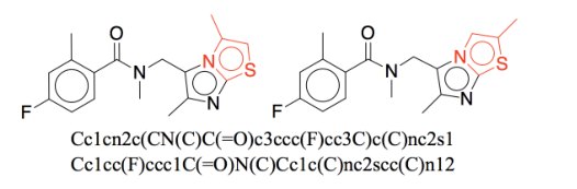
Figure 1: Two almost identical molecules with markedly different canonical SMILES in RDKit. The edit distance between two strings is 22 (50.5% of the whole sequence).
图 1:两个几乎相同的分子,在 RDKit 中的规范 SMILES 却明显不同。两个字符串的编辑距离为 22(占整个序列的 50.5%)。
Our primary contribution is a new generative model of molecular graphs. While one could imagine solving the problem in a standard manner – generating graphs node by node (Li et al. 2018) – the approach is not ideal for molecules. This is because creating molecules atom by atom would force the model to generate chemically invalid intermediaries (see, e.g., Figure 2), delaying validation until a complete graph is generated. Instead, we propose to generate molecular graphs in two phases by exploiting valid subgraphs as components. The overall generative approach, cast as a junction tree variational autoencoder[^1], first generates a tree structured object (a junction tree) whose role is to represent the scaffold of subgraph components and their coarse relative arrangements. The components are valid chemical substructures automatically extracted from the training set using tree decomposition and are used as building blocks. In the second phase, the subgraphs (nodes in the tree) are assembled together into a molecular graph.
我们的主要贡献是一种新的分子图生成模型。虽然可以想象用标准方式解决——逐节点生成图(Li 等,2018)——这对分子并不理想。因为按原子逐个创建分子会迫使模型生成化学上无效的中间物(例如见图 2),有效性要等到完整图生成后才能验证。相反,我们提议利用有效子图作为组件,分两阶段生成分子图。整体生成方法表述为连接树变分自编码器[^1]:先生成一个树状对象(连接树),用来表示子图组件的骨架及其粗粒度相对排布。这些组件是用树分解从训练集中自动抽出的有效化学子结构,并用作积木。第二阶段再把子图(树中的节点)组装成分子图。
We evaluate our model on multiple tasks ranging from molecular generation to optimization of a given molecule according to desired properties. As baselines, we utilize state-of-the-art SMILES-based generation approaches (Kusner et al. 2017; Dai et al. 2018). We demonstrate that our model produces 100% valid molecules when sampled from a prior distribution, outperforming the top performing baseline by a significant margin. In addition, we show that our model excels in discovering molecules with desired properties, yielding a 30% relative gain over the baselines.
我们在从分子生成到按所需性质优化给定分子的多项任务上评估模型。基线采用当时最优的基于 SMILES 的生成方法(Kusner 等,2017;Dai 等,2018)。我们表明,从先验分布采样时,我们的模型产生 100% 有效的分子,以明显优势超过表现最好的基线。此外,我们表明模型擅长发现具有所需性质的分子,相对基线有约 30% 的相对提升。
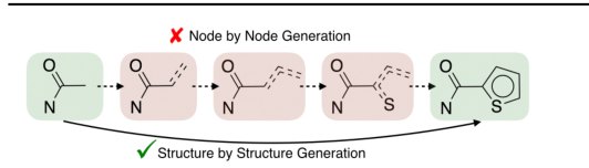
Figure 2: Comparison of two graph generation schemes: Structure by structure approach is preferred as it avoids invalid intermediate states (marked in red) encountered in node by node approach.
图 2:两种图生成方案的比较:按结构逐块生成的做法更可取,因为它避免了逐节点方法中会遇到的无效中间状态(标为红色)。
2 Junction Tree Variational Autoencoder
2 连接树变分自编码器
Our approach extends the variational autoencoder (Kingma & Welling 2013) to molecular graphs by introducing a suitable encoder and a matching decoder. Deviating from previous work (Gómez-Bombarelli et al. 2016; Kusner et al. 2017), we interpret each molecule as having been built from subgraphs chosen out of a vocabulary of valid components. These components are used as building blocks both when encoding a molecule into a vector representation as well as when decoding latent vectors back into valid molecular graphs. The key advantage of this view is that the decoder can realize a valid molecule piece by piece by utilizing the collection of valid components and how they interact, rather than trying to build the molecule atom by atom through chemically invalid intermediaries (Figure 2). An aromatic bond, for example, is chemically invalid on its own unless the entire aromatic ring is present. It would be therefore challenging to learn to build rings atom by atom rather than by introducing rings as part of the basic vocabulary.
我们的方法把变分自编码器(Kingma 与 Welling,2013)扩展到分子图,引入合适的编码器和匹配的解码器。与先前工作(Gómez-Bombarelli 等,2016;Kusner 等,2017)不同,我们把每个分子理解为由从有效组件词表中选出的子图搭建而成。这些组件既在把分子编码成向量表示时用作积木,也在把潜向量解码回有效分子图时使用。这一视角的关键优点是:解码器可以借助有效组件集合以及它们如何相互作用,一块一块地实现有效分子,而不必通过化学上无效的中间物按原子去搭建(图 2)。例如,芳香键单独并不化学有效,除非整个芳香环都在;因此,按原子去学着搭环会很难,不如把环作为基本词表的一部分引入。
Our vocabulary of components, such as rings, bonds and individual atoms, is chosen to be large enough so that a given molecule can be covered by overlapping components or clusters of atoms. The clusters serve the role analogous to cliques in graphical models, as they are expressive enough that a molecule can be covered by overlapping clusters without forming cluster cycles. In this sense, the clusters serve as cliques in a (non-optimal) triangulation of the molecular graph. We form a junction tree of such clusters and use it as the tree representation of the molecule. Since our choice of cliques is constrained a priori, we cannot guarantee that a junction tree exists with such clusters for an arbitrary molecule. However, our clusters are built on the basis of the molecules in the training set to ensure that a corresponding junction tree can be found. Empirically, our clusters cover most of the molecules in the test set.
我们的组件词表(如环、键和单个原子)选得足够大,使给定分子可以被重叠的原子组件或簇覆盖。这些簇所起的作用类似于图模型中的团:它们有足够的表达能力,使分子可以被重叠的簇覆盖而不形成簇环。在这个意义上,簇充当分子图某种(非最优)三角化中的团。我们由这些簇形成连接树,并把它用作分子的树表示。由于团的选择事先受限,我们不能保证对任意分子都存在由这类簇构成的连接树。不过,我们的簇是基于训练集中的分子构建的,以确保能找到对应的连接树。经验上,这些簇覆盖了测试集中的大多数分子。
The original molecular graph and its associated junction tree offer two complementary representations of a molecule. We therefore encode the molecule into a two-part latent representation where encodes the tree structure and what the clusters are in the tree without fully capturing how exactly the clusters are mutually connected. encodes the graph to capture the fine-grained connectivity. Both parts are created by tree and graph encoders and . The latent representation is then decoded back into a molecular graph in two stages. As illustrated in Figure 3, we first reproduce the junction tree using a tree decoder based on the information in . Second, we predict the fine grain connectivity between the clusters in the junction tree using a graph decoder to realize the full molecular graph. The junction tree approach allows us to maintain chemical feasibility during generation.
原始分子图及其关联的连接树提供了分子的两种互补表示。因此我们把分子编码成两部分潜表示 ,其中 编码树结构以及树中有哪些簇,但并不完整刻画簇之间究竟如何相连; 编码图以捕捉细粒度连接。两部分分别由树编码器 和图编码器 产生。潜表示再分两阶段解码回分子图。如图 3 所示,我们先用基于 的树解码器 复现连接树;然后用图解码器 预测连接树中各簇之间的细粒度连接,从而实现完整分子图。连接树方法使我们能在生成过程中保持化学可行性。
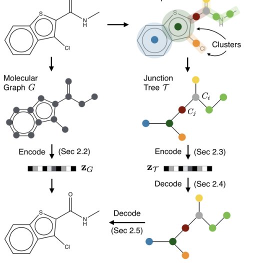
Figure 3: Overview of our method: A molecular graph is first decomposed into its junction tree , where each colored node in the tree represents a substructure in the molecule. We then encode both the tree and graph into their latent embeddings and . To decode the molecule, we first reconstruct junction tree from , and then assemble nodes in the tree back to the original molecule.
图 3:方法概览:分子图 先被分解成连接树 ,树中每个彩色节点表示分子中的一个子结构。我们再把树和图分别编码到潜嵌入 和 。解码分子时,先从 重建连接树,再把树中的节点组装回原来的分子。
Notation A molecular graph is defined as where is the set of atoms (vertices) and the set of bonds (edges). Let be the neighbor of . We denote sigmoid function as and ReLU function as . We use for nodes in the tree and for nodes in the graph.
记号 分子图定义为 ,其中 是原子(顶点)集合, 是键(边)集合。设 为 的邻居。我们把 sigmoid 函数记为 ,ReLU 函数记为 。我们用 表示树中的节点,用 表示图中的节点。
2.1 Junction Tree
2.1 连接树
A tree decomposition maps a graph into a junction tree by contracting certain vertices into a single node so that becomes cycle-free. Formally, given a graph , a junction tree is a connected labeled tree whose node set is and edge set is . Each node or cluster is an induced subgraph of , satisfying the following constraints:
树分解通过把某些顶点收缩成单个节点,把图 映射成一棵连接树,从而使 变得无环。形式地,给定图 ,连接树 是一棵连通的带标号树,其节点集为 ,边集为 。每个节点或簇 是 的一个诱导子图,并满足以下约束:
- The union of all clusters equals . That is, and .
- 所有簇的并等于 。也就是 且 。
- Running intersection: For all clusters and , if is on the path from to .
- 运行交性质:对所有簇 和 ,如果 在从 到 的路径上,则 。
Viewing induced subgraphs as cluster labels, junction trees are labeled trees with label vocabulary . By our molecule tree decomposition, contains only cycles (rings) and single edges. Thus the vocabulary size is limited ( for a standard dataset with 250K molecules).
把诱导子图看作簇标号时,连接树是带标号词表 的标号树。按我们的分子树分解, 只包含环(rings)和单边。因此词表规模有限(对含 25 万分子的标准数据集,)。
Tree Decomposition of Molecules Here we present our tree decomposition algorithm tailored for molecules, which finds its root in chemistry (Rarey & Dixon 1998). Our cluster vocabulary includes chemical structures such as bonds and rings (Figure 3). Given a graph , we first find all its simple cycles, and its edges not belonging to any cycles. Two simple rings are merged together if they have more than two overlapping atoms, as they constitute a specific structure called bridged compounds (Clayden et al. 2001). Each of those cycles or edges is considered as a cluster. Next, a cluster graph is constructed by adding edges between all intersecting clusters. Finally, we select one of its spanning trees as the junction tree of (Figure 3). As a result of ring merging, any two clusters in the junction tree have at most two atoms in common, facilitating efficient inference in the graph decoding phase. The detailed procedure is described in the supplementary.
分子的树分解 这里给出我们为分子定制的树分解算法,其源头在化学中(Rarey 与 Dixon,1998)。簇词表 包含键和环等化学结构(图 3)。给定图 ,我们先找出它的全部简单环,以及不属于任何环的边。如果两个简单环有超过两个重叠原子,就把它们合并,因为它们构成称为桥环化合物的特定结构(Clayden 等,2001)。每一个这样的环或边都被视为一个簇。接下来,在所有相交的簇之间加边,构造簇图。最后,选取它的一棵生成树作为 的连接树(图 3)。由于环的合并,连接树中任意两个簇至多有两个原子相同,这便于图解码阶段的高效推断。详细步骤见补充材料。
2.2 Graph Encoder
2.2 图编码器
We first encode the latent representation of by a graph message passing network (Dai et al. 2016; Gilmer et al. 2017). Each vertex has a feature vector indicating the atom type, valence, and other properties. Similarly, each edge has a feature vector indicating its bond type, and two hidden vectors and denoting the message from to and vice versa. Due to the loopy structure of the graph, messages are exchanged in a loopy belief propagation fashion:
我们先用图消息传递网络(Dai 等,2016;Gilmer 等,2017)编码 的潜表示。每个顶点 有特征向量 ,标明原子类型、化合价和其他性质。类似地,每条边 有特征向量 标明键类型,以及两个隐向量 和 ,分别表示从 到 以及反向的消息。由于图有环状结构,消息按带环信念传播的方式交换:
where is the message computed in -th iteration, initialized with . After steps of iteration, we aggregate those messages as the latent vector of each vertex, which captures its local graphical structure:
其中 是第 次迭代计算的消息,初始化为 。经过 步迭代后,我们把这些消息聚合成每个顶点的潜向量,以刻画其局部图结构:
The final graph representation is . The mean and log variance of the variational posterior approximation are computed from with two separate affine layers. is sampled from a Gaussian .
最终的图表示为 。变分后验近似的均值 和对数方差 由 经两个独立的仿射层算出。 从高斯 中采样。
2.3 Tree Encoder
2.3 树编码器
We similarly encode with a tree message passing network. Each cluster is represented by a one-hot encoding representing its label type. Each edge is associated with two message vectors and . We pick an arbitrary leaf node as the root and propagate messages in two phases. In the first bottom-up phase, messages are initiated from the leaf nodes and propagated iteratively towards root. In the top-down phase, messages are propagated from the root to all the leaf nodes. Message is updated as:
我们类似地用树消息传递网络编码 。每个簇 用表示其标号类型的独热编码 表示。每条边 对应两个消息向量 和 。我们任意选一个叶节点作为根,分两阶段传播消息。第一阶段自底向上:消息从叶节点出发,迭代地向根传播。自顶向下阶段则把消息从根传到所有叶节点。消息 更新为:
where GRU is a Gated Recurrent Unit (Chung et al. 2014; Li et al. 2015) adapted for tree message passing:
其中 GRU 是为树消息传递改写的门控循环单元(Chung 等,2014;Li 等,2015):
The message passing follows the schedule where is computed only when all its precursors have been computed. This architectural design is motivated by the belief propagation algorithm over trees and is thus different from the graph encoder.
消息传递遵循这样的调度: 只有在其全部前驱 都已算完时才计算。这一结构来自树上的信念传播算法,因而与图编码器不同。
After the message passing, we obtain the latent representation of each node by aggregating its inward messages:
消息传递之后,我们把每个节点的入向消息聚合,得到该节点的潜表示 :
The final tree representation is , which encodes a rooted tree . Unlike the graph encoder, we do not apply node average pooling because it confuses the tree decoder which node to generate first. is sampled in a similar way as in the graph encoder. For simplicity, we abbreviate as from now on.
最终的树表示为 ,它编码一棵有根树 。与图编码器不同,我们不做节点平均池化,因为它会让树解码器搞不清该先生成哪个节点。 的采样方式与图编码器类似。为简单起见,后文把 简写为 。
This tree encoder plays two roles in our framework. First, it is used to compute , which only requires the bottom-up phase of the network. Second, after a tree is decoded from , it is used to compute messages over the entire , to provide essential contexts of every node during graph decoding. This requires both top-down and bottom-up phases. We will elaborate this in section 2.5.
这个树编码器在我们的框架里扮演两个角色。第一,它用来计算 ,这只需要网络的自底向上阶段。第二,从 解码出树 之后,它用来在整棵 上计算消息 ,以便在图解码时为每个节点提供必要上下文。这需要自顶向下和自底向上两个阶段。我们将在 2.5 节详细说明。
2.4 Tree Decoder
2.4 树解码器
We decode a junction tree from its encoding with a tree structured decoder. The tree is constructed in a top-down fashion by generating one node at a time. As illustrated in Figure 4, our tree decoder traverses the entire tree from the root, and generates nodes in their depth-first order. For every visited node, the decoder first makes a topological prediction: whether this node has children to be generated. When a new child node is created, we predict its label and recurse this process. Recall that cluster labels represent subgraphs in a molecule. The decoder backtracks when a node has no more children to generate.
我们用树结构解码器从编码 解码出连接树 。树按自顶向下的方式一次生成一个节点。如图 4 所示,树解码器从根遍历整棵树,并按深度优先顺序生成节点。对每个访问到的节点,解码器先做一次拓扑预测:该节点是否还有待生成的子节点。当创建一个新的子节点时,我们预测它的标号并递归这一过程。回忆一下,簇标号表示分子中的子图。当一个节点不再有子节点要生成时,解码器回溯。
At each time step, a node receives information from other nodes in the current tree for making those predictions. The information is propagated through message vectors when trees are incrementally constructed. Formally, let be the edges traversed in a depth first traversal over , where as each edge is traversed in both directions. The model visits node at time . Let be the first edges in . The message is updated through previous messages:
在每个时间步,节点从当前树中的其他节点接收信息以做出这些预测。树逐步构造时,信息通过消息向量 传播。形式地,设 是在 上深度优先遍历经过的边,其中 ,因为每条边两个方向都会经过。模型在时刻 访问节点 。设 为 中的前 条边。消息 通过先前消息更新:
where GRU is the same recurrent unit as in the tree encoder.
其中 GRU 与树编码器中的循环单元相同。
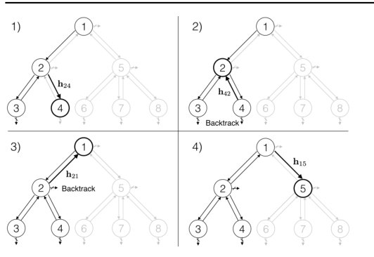
Figure 4: Illustration of the tree decoding process. Nodes are labeled in the order in which they are generated. 1) Node 2 expands child node 4 and predicts its label with message . 2) As node 4 is a leaf node, decoder backtracks and computes message . 3) Decoder continues to backtrack as node 2 has no more children. 4) Node 1 expands node 5 and predicts its label.
图 4:树解码过程示意。节点按生成顺序标号。1)节点 2 扩展出子节点 4,并用消息 预测其标号。2)由于节点 4 是叶节点,解码器回溯并计算消息 。3)节点 2 不再有子节点,解码器继续回溯。4)节点 1 扩展出节点 5 并预测其标号。
0: Latent representation
1: Initialize: Tree
2: function SampleTree()
3: Set all cluster labels that are chemically compatible with node and its current neighbors.
4: Set with probability . Eq.(11)
5: if and then
6: Create a node and add it to tree .
7: Sample the label of node from . Eq.(12)
8: SampleTree()
9: end if
10: end function
Algorithm 1 Tree decoding at sampling time
0: 潜表示
1: 初始化: 树
2: 函数 SampleTree()
3: 令 与节点 及其当前邻居在化学上相容的全部簇标号。
4: 以概率 令 。 式 (11)
5: 如果 且 则
6: 创建一个节点 并把它加入树 。
7: 从 中采样节点 的标号 。式 (12)
8: SampleTree()
9: 结束如果
10: 结束函数
算法 1 采样时的树解码
Topological Prediction When the model visits node , it makes a binary prediction on whether it still has children to be generated. We compute this probability by combining , node features and inward messages via a one hidden layer network followed by a sigmoid function:
拓扑预测 当模型访问节点 时,它做一个二值预测:该节点是否还有待生成的子节点。我们把 、节点特征 和入向消息 通过单隐层网络再接 sigmoid 函数来计算这一概率:
Label Prediction When a child node is generated from its parent , we predict its node label with
标号预测 当从父节点 生成子节点 时,我们用下式预测其节点标号
where is a distribution over label vocabulary . When is a root node, its parent is a virtual node and .
其中 是标号词表 上的分布。当 是根节点时,其父节点 是虚节点,且 。
Learning The tree decoder aims to maximize the likelihood . Let and be the ground truth topological and label values, the decoder minimizes the following cross entropy loss:[^2]
学习 树解码器的目标是最大化似然 。设 和 为真实的拓扑值和标号值,解码器最小化如下交叉熵损失:[^2]
Similar to sequence generation, during training we perform teacher forcing: after topological and label prediction at each step, we replace them with their ground truth so that the model makes predictions given correct histories.
与序列生成类似,训练时我们做教师强制:每一步做完拓扑预测和标号预测后,用真实值替换它们,使模型在正确历史条件下做预测。
Decoding & Feasibility Check Algorithm 1 shows how a tree is sampled from . The tree is constructed recursively guided by topological predictions without any external guidance used in training. To ensure the sampled tree could be realized into a valid molecule, we define set to be cluster labels that are chemically compatible with node and its current neighbors. When a child node is generated from node , we sample its label from with a renormalized distribution over by masking out invalid labels.
解码与可行性检查 算法 1 展示如何从 采样一棵树。树在拓扑预测的引导下递归构造,不再使用训练时的外部指导。为确保采样出的树能够实现为有效分子,我们把集合 定义为与节点 及其当前邻居在化学上相容的簇标号。当从节点 生成子节点 时,我们屏蔽无效标号,按在 上重新归一化的分布 采样其标号。
2.5 Graph Decoder
2.5 图解码器
The final step of our model is to reproduce a molecular graph that underlies the predicted junction tree . Note that this step is not deterministic since there are potentially many molecules that correspond to the same junction tree. The underlying degree of freedom pertains to how neighboring clusters and are attached to each other as subgraphs. Our goal here is to assemble the subgraphs (nodes in the tree) together into the correct molecular graph.
模型的最后一步是复现预测连接树 所对应的分子图 。注意这一步并不是确定性的,因为同一棵连接树可能对应许多分子。底层的自由度在于相邻簇 与 作为子图如何彼此连接。我们这里的目标是把子图(树中的节点)组装成正确的分子图。
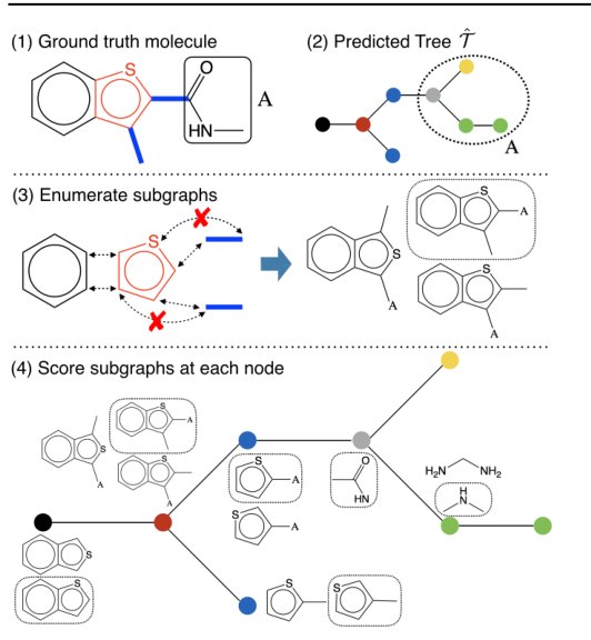
Figure 5: Decode a molecule from a junction tree. 1) Ground truth molecule . 2) Predicted junction tree . 3) We enumerate different combinations between red cluster and its neighbors. Crossed arrows indicate combinations that lead to chemically infeasible molecules. Note that if we discard tree structure during enumeration (i.e., ignoring subtree A), the last two candidates will collapse into the same molecule. 4) Rank subgraphs at each node. The final graph is decoded by putting together all the predicted subgraphs (dashed box).
图 5:从连接树解码分子。1)真实分子 。2)预测的连接树 。3)我们枚举红色簇 与其邻居之间的不同组合。打叉的箭头表示会导致化学上不可行分子的组合。注意,如果枚举时丢掉树结构(也就是忽略子树 A),最后两个候选会塌成同一个分子。4)在每个节点上给子图排序。最终的图通过把所有预测子图(虚线框)拼在一起解码得到。
Let be the set of graphs whose junction tree is . Decoding graph from is a structured prediction:
设 为连接树为 的图的集合。从 解码图 是一个结构化预测问题:
where is a scoring function over candidate graphs. We only consider scoring functions that decompose across the clusters and their neighbors. In other words, each term in the scoring function depends only on how a cluster is attached to its neighboring clusters , in the tree . The problem of finding the highest scoring graph – the assembly task – could be cast as a graphical model inference task in a model induced by the junction tree. However, for efficiency reasons, we will assemble the molecular graph one neighborhood at a time, following the order in which the tree itself was decoded. In other words, we start by sampling the assembly of the root and its neighbors according to their scores. Then we proceed to assemble the neighbors and their associated clusters (removing the degrees of freedom set by the root assembly), and so on.
其中 是候选图上的打分函数。我们只考虑能在各簇及其邻居上分解的打分函数。换句话说,打分函数的每一项只依赖于簇 如何连接到树 中的相邻簇 ,。寻找得分最高的图 (组装任务)可以表述为由连接树诱导的图模型推断。不过出于效率,我们将按树本身被解码的顺序,一次组装一个邻域。也就是说,我们先按得分采样根及其邻居的组装方式,然后继续组装这些邻居及其相关簇(去掉根组装已经固定的自由度),依此类推。
It remains to be specified how each neighborhood realization is scored. Let be the subgraph resulting from a particular merging of cluster in the tree with its neighbors , . We score as a candidate subgraph by first deriving a vector representation and then using as the subgraph score. To this end, let specify atoms in the candidate subgraph and let if and if . The indices are used to mark the position of the atoms in the junction tree, and to retrieve messages summarizing the subtree under along the edge obtained by running the tree encoding algorithm. The neural messages pertaining to the atoms and bonds in subgraph are obtained and aggregated into , similarly to the encoding step, but with different (learned) parameters:
接下来需要说明每个邻域实现如何打分。设 是把树中的簇 与其邻居 ()按某种方式合并得到的子图。我们先导出向量表示 ,再用 作为子图得分,从而给候选子图 打分。为此,设 指定候选子图 中的原子,并令 若 , 若 。下标 用来标记原子在连接树中的位置,并检索通过运行树编码算法得到的、沿边 汇总 下方子树的消息 。子图 中与原子和键相关的神经消息被求出并聚合成 ,方式与编码步骤类似,但使用不同的(可学习)参数:
$$\displaystyle\boldsymbol{\mu}{uv}^{(t)} \ \displaystyle= \ \displaystyle\tau(\mathbf{W}{1}^{a}\mathbf{x}{u}+\mathbf{W}{2}^{a}\mathbf{x}{uv}+\mathbf{W}{3}^{a}\widetilde{\boldsymbol{\mu}}{uv}^{(t-1)}) \ \displaystyle\widetilde{\boldsymbol{\mu}}{uv}^{(t-1)} \ \displaystyle= \ \displaystyle\begin{cases}\sum_{w\in N(u)\backslash v}\boldsymbol{\mu}{wu}^{(t-1)}&\alpha{u}=\alpha_{v}\
\widehat{\mathbf{m}}{\alpha{u},\alpha_{v}}+\sum_{w\in N(u)\backslash v}\boldsymbol{\mu}{wu}^{(t-1)}&\alpha{u}\neq\alpha_{v}\end{cases} \tag{15}$$
The major difference from Eq. (1) is that we augment the model with tree messages derived by running the tree encoder over the predicted tree . provides a tree dependent positional context for bond (illustrated as subtree A in Figure 5).
与式 (1) 的主要差别是:我们用在预测树 上运行树编码器得到的树消息 来增强模型。 为键 提供依赖于树的位置上下文(图 5 中表示为子树 A)。
Learning The graph decoder parameters are learned to maximize the log-likelihood of predicting correct subgraphs of the ground true graph at each tree node:
学习 图解码器的参数通过最大化在每个树节点上预测真实图 的正确子图 的对数似然来学习:
where is the set of possible candidate subgraphs at tree node . During training, we again apply teacher forcing, i.e. we feed the graph decoder with ground truth trees as input.
其中 是树节点 处可能的候选子图集合。训练时我们再次使用教师强制,也就是把真实树作为输入喂给图解码器。
Complexity By our tree decomposition, any two clusters share at most two atoms, so we only need to merge at most two atoms or one bond. By pruning chemically invalid subgraphs and merging isomorphic graphs, on average when tested on a standard ZINC drug dataset. The computational complexity of JT-VAE is therefore linear in the number of clusters, scaling nicely to large graphs.
复杂度 按我们的树分解,任意两个簇至多共享两个原子,因此只需合并至多两个原子或一条键。通过剪掉化学上无效的子图并合并同构图,在标准 ZINC 药物数据集上测试时, 平均约为 4。因此 JT-VAE 的计算复杂度对簇数呈线性,能够很好地扩展到大图。
3 Experiments
3 实验
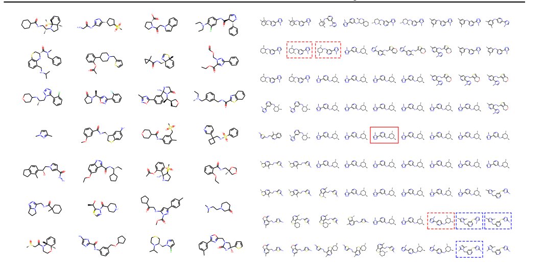
Figure 6: Left: Random molecules sampled from prior distribution . Right: Visualization of the local neighborhood of a molecule in the center. Three molecules highlighted in red dashed box have the same tree structure as the center molecule, but with different graph structure as their clusters are combined differently. The same phenomenon emerges in another group of molecules (blue dashed box).
图 6:左:从先验分布 采样的随机分子。右:中心分子局部邻域的可视化。红色虚线框标出的三个分子与中心分子具有相同的树结构,但由于簇的组合方式不同而图结构不同。同一现象也出现在另一组分子中(蓝色虚线框)。
Our evaluation efforts measure various aspects of molecular generation. The first two evaluations follow previously proposed tasks (Kusner et al. 2017). We also introduce a third task — constrained molecule optimization.
我们的评估衡量分子生成的多个方面。前两项评估沿用先前提出的任务(Kusner 等,2017)。我们还引入第三项任务——带约束的分子优化。
- • Molecule reconstruction and validity We test the VAE models on the task of reconstructing input molecules from their latent representations, and decoding valid molecules when sampling from prior distribution. (Section 3.1)
- • 分子重建与有效性 我们在从潜表示重建输入分子、以及从先验分布采样时解码出有效分子这两项上测试各 VAE 模型。(3.1 节)
- • Bayesian optimization Moving beyond generating valid molecules, we test how the model can produce novel molecules with desired properties. To this end, we perform Bayesian optimization in the latent space to search molecules with specified properties. (Section 3.2)
- • 贝叶斯优化 在生成有效分子之外,我们测试模型能否产生具有所需性质的新分子。为此,我们在潜空间中做贝叶斯优化,搜索具有指定性质的分子。(3.2 节)
- • Constrained molecule optimization The task is to modify given molecules to improve specified properties, while constraining the degree of deviation from the original molecule. This is a more realistic scenario in drug discovery, where development of new drugs usually starts with known molecules such as existing drugs (Besnard et al. 2012). Since it is a new task, we cannot compare to any existing baselines. (Section 3.3)
- • 带约束的分子优化 任务是修改给定分子以改善指定性质,同时限制相对原分子的偏离程度。这更接近药物发现中的现实情形:新药开发通常从已知分子(例如已有药物)出发(Besnard 等,2012)。由于这是新任务,我们无法与已有基线比较。(3.3 节)
Below we describe the data, baselines and model configuration that are shared across the tasks. Additional setup details are provided in the task-specific sections.
下面描述各任务共用的数据、基线和模型配置。更多设置细节见各任务专节。
Data We use the ZINC molecule dataset from Kusner et al. 2017 for our experiments, with the same training/testing split. It contains about 250K drug molecules extracted from the ZINC database (Sterling & Irwin 2015). We follow the same train/test split as in Kusner et al. 2017.
数据 实验使用 Kusner 等(2017)中的 ZINC 分子数据集,并采用相同的训练/测试划分。它包含从 ZINC 数据库(Sterling 与 Irwin,2015)抽出的约 25 万个药物分子。训练/测试划分与 Kusner 等(2017)相同。
Baselines We compare our approach with SMILES-based baselines: 1) Character VAE (CVAE) (Gómez-Bombarelli et al. 2016) which generates SMILES strings character by character; 2) Grammar VAE (GVAE) (Kusner et al. 2017) that generates SMILES following syntactic constraints given by a context-free grammar; 3) Syntax-directed VAE (SD-VAE) (Dai et al. 2018) that incorporates both syntactic and semantic constraints of SMILES via attribute grammar. For molecule generation task, we also compare with GraphVAE (Simonovsky & Komodakis 2018) that directly generates atom labels and adjacency matrices of graphs, as well as an LSTM-based autoregressive model that generates molecular graphs atom by atom (Li et al. 2018).
基线 我们与基于 SMILES 的基线比较:1)字符 VAE(CVAE)(Gómez-Bombarelli 等,2016),逐字符生成 SMILES 字符串;2)语法 VAE(GVAE)(Kusner 等,2017),按上下文无关文法给出的句法约束生成 SMILES;3)句法指导 VAE(SD-VAE)(Dai 等,2018),通过属性文法同时纳入 SMILES 的句法和语义约束。在分子生成任务上,我们还与直接生成原子标号和邻接矩阵的 GraphVAE(Simonovsky 与 Komodakis,2018),以及逐原子生成分子图的基于 LSTM 的自回归模型(Li 等,2018)比较。
Model Configuration To be comparable with the above baselines, we set the latent space dimension as 56, i.e., the tree and graph representation and have 28 dimensions each. Full training details and model configurations are provided in the appendix.
模型配置 为与上述基线可比,我们把潜空间维数设为 56,也就是树表示 和图表示 各 28 维。完整训练细节和模型配置见附录。
3.1 Molecule Reconstruction and Validity
3.1 分子重建与有效性
Setup The first task is to reconstruct and sample molecules from latent space. Since both encoding and decoding process are stochastic, we estimate reconstruction accuracy by Monte Carlo method used in (Kusner et al. 2017): Each molecule is encoded 10 times and each encoding is decoded 10 times. We report the portion of the 100 decoded molecules that are identical to the input molecule.
设置 第一项任务是从潜空间重建并采样分子。由于编码和解码过程都是随机的,我们用 Kusner 等(2017)中的蒙特卡洛方法估计重建准确率:每个分子编码 10 次,每次编码再解码 10 次。我们报告这 100 个解码分子中与输入分子相同的比例。
To compute validity, we sample 1000 latent vectors from the prior distribution , and decode each of these vectors 100 times. We report the percentage of decoded molecules that are chemically valid (checked by RDKit). For ablation study, we also report the validity of our model without validity check in decoding phase.
为计算有效性,我们从先验分布 采样 1000 个潜向量,并把每个向量解码 100 次。我们报告解码分子中化学有效的百分比(由 RDKit 检查)。作为消融,我们也报告解码阶段不做有效性检查时模型的有效性。
Results Table 1 shows that JT-VAE outperforms previous models in molecule reconstruction, and always produces valid molecules when sampled from prior distribution. In contrast, the atom-by-atom based generation only achieves 89.2% validity as it needs to go through invalid intermediate states (Figure 2). Our model bypasses this issue by utilizing valid substructures as building blocks. As shown in Figure 6, the sampled molecules have non-trivial structures such as simple chains. We further sampled 5000 molecules from prior and found they are all distinct from the training set. Thus our model is not a simple memorization.
结果 表 1 表明,JT-VAE 在分子重建上超过先前模型,并且从先验采样时总是产生有效分子。相反,逐原子生成只达到 89.2% 的有效性,因为它必须经过无效的中间状态(图 2)。我们的模型通过把有效子结构当作积木来绕开这一问题。如图 6 所示,采样出的分子具有并非平凡的结构,例如简单链。我们进一步从先验采样了 5000 个分子,发现它们与训练集全部不同。因此我们的模型并不是简单的记忆。
| Method | Reconstruction | Validity |
|---|---|---|
| CVAE | 44.6% | 0.7% |
| GVAE | 53.7% | 7.2% |
| SD-VAE | 76.2% | 43.5% |
| GraphVAE | - | 13.5% |
| Atom-by-Atom LSTM | - | 89.2% |
| JT-VAE | 76.7% | 100.0% |
Table 1: Reconstruction accuracy and prior validity results. Baseline results are copied from Kusner et al. 2017; Dai et al. 2018; Simonovsky & Komodakis 2018; Li et al. 2018.
| 方法 | 重建 | 有效性 |
|---|---|---|
| CVAE | 44.6% | 0.7% |
| GVAE | 53.7% | 7.2% |
| SD-VAE | 76.2% | 43.5% |
| GraphVAE | - | 13.5% |
| 逐原子 LSTM | - | 89.2% |
| JT-VAE | 76.7% | 100.0% |
表 1:重建准确率与先验有效性结果。基线结果引自 Kusner 等,2017;Dai 等,2018;Simonovsky 与 Komodakis,2018;Li 等,2018。
Analysis We qualitatively examine the latent space of JT-VAE by visualizing the neighborhood of molecules. Given a molecule, we follow the method in Kusner et al. 2017 to construct a grid visualization of its neighborhood. Figure 6 shows the local neighborhood of the same molecule visualized in Dai et al. 2018. In comparison, our neighborhood does not contain molecules with huge rings (with more than 7 atoms), which rarely occur in the dataset. We also highlight two groups of closely resembling molecules that have identical tree structures but vary only in how clusters are attached together. This demonstrates the smoothness of learned molecular embeddings.
分析 我们通过可视化分子邻域来定性考察 JT-VAE 的潜空间。给定一个分子,我们按 Kusner 等(2017)的方法构造其邻域的网格可视化。图 6 展示了 Dai 等(2018)中同一分子的局部邻域。相比之下,我们的邻域不包含很大的环(超过 7 个原子),这类结构在数据集中很少出现。我们还标出两组非常相近的分子:它们具有相同的树结构,只是簇如何连接有所不同。这表明学到的分子嵌入是平滑的。
3.2 Bayesian Optimization
3.2 贝叶斯优化
Setup The second task is to produce novel molecules with desired properties. Following (Kusner et al. 2017), our target chemical property is octanol-water partition coefficients (logP) penalized by the synthetic accessibility (SA) score and number of long cycles.[^3] To perform Bayesian optimization (BO), we first train a VAE and associate each molecule with a latent vector, given by the mean of the variational encoding distribution. After the VAE is learned, we train a sparse Gaussian process (SGP) to predict given its latent representation. Then we perform five iterations of batched BO using the expected improvement heuristic.
设置 第二项任务是产生具有所需性质的新分子。沿用 Kusner 等(2017),我们的目标化学性质 是用合成可及性(SA)分数和长环数目惩罚后的辛醇–水分配系数(logP)。[^3] 为做贝叶斯优化(BO),我们先训练一个 VAE,并把每个分子与一个潜向量关联,该向量取变分编码分布的均值。VAE 学好之后,我们训练一个稀疏高斯过程(SGP),根据潜表示预测 。然后我们用期望改进启发式做五轮批量 BO。
For comparison, we report 1) the predictive performance of SGP trained on latent encodings learned by different VAEs, measured by log-likelihood (LL) and root mean square error (RMSE) with 10-fold cross validation. 2) The top-3 molecules found by BO under different models.
为便于比较,我们报告:1)在不同 VAE 学到的潜编码上训练的 SGP 的预测表现,用 10 折交叉验证的对数似然(LL)和均方根误差(RMSE)衡量;2)不同模型经 BO 找到的前 3 个分子。
Results As shown in Table 2, JT-VAE finds molecules with significantly better scores than previous methods. Figure 7 lists the top-3 best molecules found by JT-VAE. In fact, JT-VAE finds over 50 molecules with scores over 3.50 (the second best molecule proposed by SD-VAE). Moreover, the SGP yields better predictive performance when trained on JT-VAE embeddings (Table 3).
结果 如表 2 所示,JT-VAE 找到的分子分数显著好于先前方法。图 7 列出 JT-VAE 找到的最好的 3 个分子。实际上,JT-VAE 找到了 50 多个分数超过 3.50 的分子(这是 SD-VAE 提出的第二好分子的分数)。此外,在 JT-VAE 嵌入上训练的 SGP 预测表现也更好(表 3)。
| Method | 1st | 2nd | 3rd |
|---|---|---|---|
| CVAE | 1.98 | 1.42 | 1.19 |
| GVAE | 2.94 | 2.89 | 2.80 |
| SD-VAE | 4.04 | 3.50 | 2.96 |
| JT-VAE | 5.30 | 4.93 | 4.49 |
Table 2: Best molecule property scores found by each method. Baseline results are from Kusner et al. 2017; Dai et al. 2018.
| 方法 | 第 1 | 第 2 | 第 3 |
|---|---|---|---|
| CVAE | 1.98 | 1.42 | 1.19 |
| GVAE | 2.94 | 2.89 | 2.80 |
| SD-VAE | 4.04 | 3.50 | 2.96 |
| JT-VAE | 5.30 | 4.93 | 4.49 |
表 2:各方法找到的最好分子性质分数。基线结果来自 Kusner 等,2017;Dai 等,2018。
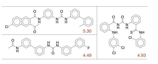
Figure 7: Best three molecules and their property scores found by JT-VAE using Bayesian optimization.
图 7:用贝叶斯优化、由 JT-VAE 找到的最好的三个分子及其性质分数。
| Method | LL | RMSE |
|---|---|---|
| CVAE | ||
| GVAE | ||
| SD-VAE | ||
| JT-VAE |
Table 3: Predictive performance of sparse Gaussian Processes trained on different VAEs. Baseline results are copied from Kusner et al. 2017 and Dai et al. 2018.
| 方法 | LL | RMSE |
|---|---|---|
| CVAE | ||
| GVAE | ||
| SD-VAE | ||
| JT-VAE |
表 3:在不同 VAE 上训练的稀疏高斯过程的预测表现。基线结果引自 Kusner 等,2017 和 Dai 等,2018。
| Improvement | Similarity | Success | |
|---|---|---|---|
| 0.0 | 97.5% | ||
| 0.2 | 97.1% | ||
| 0.4 | 83.6% | ||
| 0.6 | 46.4% |
Table 4: Constrained optimization result of JT-VAE: mean and standard deviation of property improvement, molecular similarity and success rate under constraints with varied .
| 改善 | 相似度 | 成功率 | |
|---|---|---|---|
| 0.0 | 97.5% | ||
| 0.2 | 97.1% | ||
| 0.4 | 83.6% | ||
| 0.6 | 46.4% |
表 4:JT-VAE 的带约束优化结果:在约束 且 取不同值时,性质改善、分子相似度和成功率的均值与标准差。

Figure 8: A molecule modification that yields an improvement of 4.0 with molecular similarity 0.617 (modified part is in red).
图 8:一次使性质改善 4.0、分子相似度为 0.617 的分子修改(修改部分标为红色)。
3.3 Constrained Optimization
3.3 带约束的优化
Setup The third task is to perform molecule optimization in a constrained scenario. Given a molecule , the task is to find a different molecule that has the highest property value with the molecular similarity for some threshold . We use Tanimoto similarity with Morgan fingerprint (Rogers & Hahn 2010) as the similarity metric, and penalized logP coefficient as our target chemical property. For this task, we jointly train a property predictor (parameterized by a feed-forward network) with JT-VAE to predict from the latent embedding of . To optimize a molecule , we start from its latent representation, and apply gradient ascent in the latent space to improve the predicted score , similar to (Mueller et al. 2017). After applying gradient steps, molecules are decoded from resulting latent trajectories, and we report the molecule with the highest that satisfies the similarity constraint. A modification succeeds if one of the decoded molecules satisfies the constraint and is distinct from the original.
设置 第三项任务是在带约束的情形下做分子优化。给定分子 ,任务是找到另一个分子 ,使其性质值最高,同时分子相似度 ( 为某个阈值)。我们用带 Morgan 指纹的 Tanimoto 相似度(Rogers 与 Hahn,2010)作为相似度度量,并以惩罚后的 logP 系数作为目标化学性质。对这一任务,我们用前馈网络参数化的性质预测器 与 JT-VAE 联合训练,从 的潜嵌入预测 。为优化分子 ,我们从其潜表示出发,在潜空间中做梯度上升以提高预测分数 ,做法类似 Mueller 等(2017)。经过 步梯度之后,从得到的潜轨迹解码出 个分子,并报告满足相似度约束且 最高的那个。如果解码出的分子中有一个满足约束且与原分子不同,则这次修改算成功。
To provide the greatest challenge, we selected 800 molecules with the lowest property score from the test set. We report the success rate (how often a modification succeeds), and among success cases the average improvement and molecular similarity between the original and modified molecules and .
为提供最大挑战,我们从测试集中选出性质分数 最低 的 800 个分子。我们报告成功率(修改成功的频率),以及在成功情形中原分子与修改后分子 和 之间的平均改善 和分子相似度 。
Results Our results are summarized in Table 4. The unconstrained scenario () has the best average improvement, but often proposes dissimilar molecules. When we tighten the constraint to , about 80% of the time our model finds similar molecules, with an average improvement . This also demonstrates the smoothness of the learned latent space. Figure 8 illustrates an effective modification resulting in a similar molecule with great improvement.
结果 结果汇总于表 4。无约束情形()平均改善最好,但常常提出不相似的分子。当把约束收紧到 时,大约 80% 的情况下模型能找到相似分子,平均改善为 0.84。这也表明学到的潜空间是平滑的。图 8 展示了一次有效的修改:得到一个相似且改善很大的分子。
4 Related Work
4 相关工作
Molecule Generation Previous work on molecule generation mostly operates on SMILES strings. Gómez-Bombarelli et al. 2016; Segler et al. 2017 built generative models of SMILES strings with recurrent decoders. Unfortunately, these models could generate invalid SMILES that do not result in any molecules. To remedy this issue, Kusner et al. 2017; Dai et al. 2018 complemented the decoder with syntactic and semantic constraints of SMILES by context free and attribute grammars, but these grammars do not fully capture chemical validity. Other techniques such as active learning (Janz et al. 2017) and reinforcement learning (Guimaraes et al. 2017) encourage the model to generate valid SMILES through additional training signal. Very recently, Simonovsky & Komodakis 2018 proposed to generate molecular graphs by predicting their adjacency matrices, and Li et al. 2018 generated molecules node by node. In comparison, our method enforces chemical validity and is more efficient due to the coarse-to-fine generation.
分子生成 先前的分子生成工作大多在 SMILES 字符串上操作。Gómez-Bombarelli 等(2016)和 Segler 等(2017)用循环解码器建立 SMILES 字符串的生成模型。可惜这些模型可能生成无效的 SMILES,得不到任何分子。为弥补这一点,Kusner 等(2017)和 Dai 等(2018)用上下文无关文法和属性文法给解码器补上 SMILES 的句法和语义约束,但这些文法并不能完整刻画化学有效性。主动学习(Janz 等,2017)和强化学习(Guimaraes 等,2017)等技术则通过额外训练信号鼓励模型生成有效 SMILES。最近,Simonovsky 与 Komodakis(2018)提议通过预测邻接矩阵来生成分子图,Li 等(2018)则逐节点生成分子。相比之下,我们的方法强制化学有效性,并由于粗到细的生成而更高效。
Graph-structured Encoders The neural network formulation on graphs was first proposed by Gori et al. 2005; Scarselli et al. 2009, and later enhanced by Li et al. 2015 with gated recurrent units. For recurrent architectures over graphs, Lei et al. 2017 designed Weisfeiler-Lehman kernel network inspired by graph kernels. Dai et al. 2016 considered a different architecture where graphs were viewed as latent variable graphical models, and derived their model from message passing algorithms. Our tree and graph encoder are closely related to this graphical model perspective, and to neural message passing networks (Gilmer et al. 2017). For convolutional architectures, Duvenaud et al. 2015 introduced a convolution-like propagation on molecular graphs, which was generalized to other domains by Niepert et al. 2016. Bruna et al. 2013; Henaff et al. 2015 developed graph convolution in spectral domain via graph Laplacian. For applications, graph neural networks are used in semi-supervised classification (Kipf & Welling 2016), computer vision (Monti et al. 2016), and chemical domains (Kearnes et al. 2016; Schütt et al. 2017; Jin et al. 2017).
图结构编码器 图上的神经网络表述最早由 Gori 等(2005)和 Scarselli 等(2009)提出,后来 Li 等(2015)用门控循环单元加以增强。对于图上的循环架构,Lei 等(2017)受图核启发设计了 Weisfeiler-Lehman 核网络。Dai 等(2016)考虑了另一种架构:把图看成潜变量图模型,并从消息传递算法导出他们的模型。我们的树编码器和图形编码器与这一图模型视角以及神经消息传递网络(Gilmer 等,2017)密切相关。对于卷积架构,Duvenaud 等(2015)在分子图上引入了类似卷积的传播,并由 Niepert 等(2016)推广到其他领域。Bruna 等(2013)和 Henaff 等(2015)通过图拉普拉斯在谱域发展了图卷积。在应用方面,图神经网络被用于半监督分类(Kipf 与 Welling,2016)、计算机视觉(Monti 等,2016)以及化学领域(Kearnes 等,2016;Schütt 等,2017;Jin 等,2017)。
Tree-structured Models Our tree encoder is related to recursive neural networks and tree-LSTM (Socher et al. 2013; Tai et al. 2015; Zhu et al. 2015). These models encode tree structures where nodes in the tree are bottom-up transformed into vector representations. In contrast, our model propagates information both bottom-up and top-down.
树结构模型 我们的树编码器与递归神经网络和 tree-LSTM 相关(Socher 等,2013;Tai 等,2015;Zhu 等,2015)。这些模型编码树结构,树中节点自底向上变换成向量表示。相反,我们的模型同时自底向上和自顶向下传播信息。
On the decoding side, tree generation naturally arises in natural language parsing (Dyer et al. 2016; Kiperwasser & Goldberg 2016). Different from our approach, natural language parsers have access to input words and only predict the topology of the tree. For general purpose tree generation, Vinyals et al. 2015; Aharoni & Goldberg 2017 applied recurrent networks to generate linearized version of trees, but their architectures were entirely sequence-based. Dong & Lapata 2016; Alvarez-Melis & Jaakkola 2016 proposed tree-based architectures that construct trees top-down from the root. Our model is most closely related to Alvarez-Melis & Jaakkola 2016 that disentangles topological prediction from label prediction, but we generate nodes in a depth-first order and have additional steps that propagate information bottom-up. This forward-backward propagation also appears in Parisotto et al. 2016, but their model is node based whereas ours is based on message passing.
在解码一侧,树生成自然出现在自然语言句法分析中(Dyer 等,2016;Kiperwasser 与 Goldberg,2016)。与我们的方法不同,自然语言句法分析器可以利用输入词,只需预测树的拓扑。对于通用的树生成,Vinyals 等(2015)以及 Aharoni 与 Goldberg(2017)用循环网络生成树的线性化版本,但其架构完全基于序列。Dong 与 Lapata(2016)以及 Alvarez-Melis 与 Jaakkola(2016)提出从根自顶向下构造树的基于树的架构。我们的模型与 Alvarez-Melis 与 Jaakkola(2016)最为接近,后者把拓扑预测与标号预测分开;但我们按深度优先顺序生成节点,并有额外的自底向上信息传播步骤。这种前向–后向传播也出现在 Parisotto 等(2016)中,不过他们的模型基于节点,而我们基于消息传递。
5 Conclusion
5 结论
In this paper we present a junction tree variational autoencoder for generating molecular graphs. Our method significantly outperforms previous work in molecule generation and optimization. For future work, we attempt to generalize our method for general low-treewidth graphs.
本文提出一种用于生成分子图的连接树变分自编码器。我们的方法在分子生成和优化上显著超过先前工作。未来工作中,我们尝试把方法推广到一般的低树宽图。
Acknowledgement
致谢
We thank Jonas Mueller, Chengtao Li, Tao Lei and MIT NLP Group for their helpful comments. This work was supported by the DARPA Make-It program under contract ARO W911NF-16-2-0023.
我们感谢 Jonas Mueller、Chengtao Li、Tao Lei 以及 MIT NLP Group 的有益评论。本工作由 DARPA Make-It 计划资助,合同编号 ARO W911NF-16-2-0023。
References
参考文献
Aharoni & Goldberg (2017) Aharoni, R. and Goldberg, Y. Towards string-to-tree neural machine translation. arXiv preprint arXiv:1704.04743 , 2017.
Alvarez-Melis & Jaakkola (2016) Alvarez-Melis, D. and Jaakkola, T. S. Tree-structured decoding with doubly-recurrent neural networks. 2016.
Besnard et al. (2012) Besnard, J., Ruda, G. F., Setola, V., Abecassis, K., Rodriguiz, R. M., Huang, X.-P., Norval, S., Sassano, M. F., Shin, A. I., Webster, L. A., et al. Automated design of ligands to polypharmacological profiles. Nature , 492(7428):215–220, 2012.
Bruna et al. (2013) Bruna, J., Zaremba, W., Szlam, A., and LeCun, Y. Spectral networks and locally connected networks on graphs. arXiv preprint arXiv:1312.6203 , 2013.
Chung et al. (2014) Chung, J., Gulcehre, C., Cho, K., and Bengio, Y. Empirical evaluation of gated recurrent neural networks on sequence modeling. arXiv preprint arXiv:1412.3555 , 2014.
Clayden et al. (2001) Clayden, J., Greeves, N., Warren, S., and Wothers, P. Organic Chemistry . Oxford University Press, 2001.
Dai et al. (2016) Dai, H., Dai, B., and Song, L. Discriminative embeddings of latent variable models for structured data. In International Conference on Machine Learning , pp. 2702–2711, 2016.
Dai et al. (2018) Dai, H., Tian, Y., Dai, B., Skiena, S., and Song, L. Syntax-directed variational autoencoder for structured data. International Conference on Learning Representations , 2018. URL https://openreview.net/forum?id=SyqShMZRb .
Dong & Lapata (2016) Dong, L. and Lapata, M. Language to logical form with neural attention. arXiv preprint arXiv:1601.01280 , 2016.
Duvenaud et al. (2015) Duvenaud, D. K., Maclaurin, D., Iparraguirre, J., Bombarell, R., Hirzel, T., Aspuru-Guzik, A., and Adams, R. P. Convolutional networks on graphs for learning molecular fingerprints. In Advances in neural information processing systems , pp. 2224–2232, 2015.
Dyer et al. (2016) Dyer, C., Kuncoro, A., Ballesteros, M., and Smith, N. A. Recurrent neural network grammars. arXiv preprint arXiv:1602.07776 , 2016.
Gilmer et al. (2017) Gilmer, J., Schoenholz, S. S., Riley, P. F., Vinyals, O., and Dahl, G. E. Neural message passing for quantum chemistry. arXiv preprint arXiv:1704.01212 , 2017.
Gómez-Bombarelli et al. (2016) Gómez-Bombarelli, R., Wei, J. N., Duvenaud, D., Hernández-Lobato, J. M., Sánchez-Lengeling, B., Sheberla, D., Aguilera-Iparraguirre, J., Hirzel, T. D., Adams, R. P., and Aspuru-Guzik, A. Automatic chemical design using a data-driven continuous representation of molecules. ACS Central Science , 2016. doi: 10.1021/acscentsci.7b00572 .
Gori et al. (2005) Gori, M., Monfardini, G., and Scarselli, F. A new model for learning in graph domains. In Neural Networks, 2005. IJCNN’05. Proceedings. 2005 IEEE International Joint Conference on , volume 2, pp. 729–734. IEEE, 2005.
Guimaraes et al. (2017) Guimaraes, G. L., Sanchez-Lengeling, B., Farias, P. L. C., and Aspuru-Guzik, A. Objective-reinforced generative adversarial networks (organ) for sequence generation models. arXiv preprint arXiv:1705.10843 , 2017.
Henaff et al. (2015) Henaff, M., Bruna, J., and LeCun, Y. Deep convolutional networks on graph-structured data. arXiv preprint arXiv:1506.05163 , 2015.
Janz et al. (2017) Janz, D., van der Westhuizen, J., and Hernández-Lobato, J. M. Actively learning what makes a discrete sequence valid. arXiv preprint arXiv:1708.04465 , 2017.
Jin et al. (2017) Jin, W., Coley, C., Barzilay, R., and Jaakkola, T. Predicting organic reaction outcomes with weisfeiler-lehman network. In Advances in Neural Information Processing Systems , pp. 2604–2613, 2017.
Kearnes et al. (2016) Kearnes, S., McCloskey, K., Berndl, M., Pande, V., and Riley, P. Molecular graph convolutions: moving beyond fingerprints. Journal of computer-aided molecular design , 30(8):595–608, 2016.
Kingma & Welling (2013) Kingma, D. P. and Welling, M. Auto-encoding variational bayes. arXiv preprint arXiv:1312.6114 , 2013.
Kiperwasser & Goldberg (2016) Kiperwasser, E. and Goldberg, Y. Easy-first dependency parsing with hierarchical tree lstms. arXiv preprint arXiv:1603.00375 , 2016.
Kipf & Welling (2016) Kipf, T. N. and Welling, M. Semi-supervised classification with graph convolutional networks. arXiv preprint arXiv:1609.02907 , 2016.
Kusner et al. (2017) Kusner, M. J., Paige, B., and Hernández-Lobato, J. M. Grammar variational autoencoder. arXiv preprint arXiv:1703.01925 , 2017.
Landrum (2006) Landrum, G. Rdkit: Open-source cheminformatics. Online). http://www. rdkit. org. Accessed , 3(04):2012, 2006.
Lei et al. (2017) Lei, T., Jin, W., Barzilay, R., and Jaakkola, T. Deriving neural architectures from sequence and graph kernels. arXiv preprint arXiv:1705.09037 , 2017.
Li et al. (2015) Li, Y., Tarlow, D., Brockschmidt, M., and Zemel, R. Gated graph sequence neural networks. arXiv preprint arXiv:1511.05493 , 2015.
Li et al. (2018) Li, Y., Vinyals, O., Dyer, C., Pascanu, R., and Battaglia, P. Learning deep generative models of graphs. arXiv preprint arXiv:1803.03324 , 2018.
Monti et al. (2016) Monti, F., Boscaini, D., Masci, J., Rodolà, E., Svoboda, J., and Bronstein, M. M. Geometric deep learning on graphs and manifolds using mixture model cnns. arXiv preprint arXiv:1611.08402 , 2016.
Mueller et al. (2017) Mueller, J., Gifford, D., and Jaakkola, T. Sequence to better sequence: continuous revision of combinatorial structures. In International Conference on Machine Learning , pp. 2536–2544, 2017.
Niepert et al. (2016) Niepert, M., Ahmed, M., and Kutzkov, K. Learning convolutional neural networks for graphs. In International Conference on Machine Learning , pp. 2014–2023, 2016.
Parisotto et al. (2016) Parisotto, E., Mohamed, A.-r., Singh, R., Li, L., Zhou, D., and Kohli, P. Neuro-symbolic program synthesis. arXiv preprint arXiv:1611.01855 , 2016.
Rarey & Dixon (1998) Rarey, M. and Dixon, J. S. Feature trees: a new molecular similarity measure based on tree matching. Journal of computer-aided molecular design , 12(5):471–490, 1998.
Rogers & Hahn (2010) Rogers, D. and Hahn, M. Extended-connectivity fingerprints. Journal of chemical information and modeling , 50(5):742–754, 2010.
Scarselli et al. (2009) Scarselli, F., Gori, M., Tsoi, A. C., Hagenbuchner, M., and Monfardini, G. The graph neural network model. IEEE Transactions on Neural Networks , 20(1):61–80, 2009.
Schütt et al. (2017) Schütt, K., Kindermans, P.-J., Felix, H. E. S., Chmiela, S., Tkatchenko, A., and Müller, K.-R. Schnet: A continuous-filter convolutional neural network for modeling quantum interactions. In Advances in Neural Information Processing Systems , pp. 992–1002, 2017.
Segler et al. (2017) Segler, M. H., Kogej, T., Tyrchan, C., and Waller, M. P. Generating focussed molecule libraries for drug discovery with recurrent neural networks. arXiv preprint arXiv:1701.01329 , 2017.
Simonovsky & Komodakis (2018) Simonovsky, M. and Komodakis, N. Graphvae: Towards generation of small graphs using variational autoencoders. arXiv preprint arXiv:1802.03480 , 2018.
Socher et al. (2013) Socher, R., Perelygin, A., Wu, J., Chuang, J., Manning, C. D., Ng, A., and Potts, C. Recursive deep models for semantic compositionality over a sentiment treebank. In Proceedings of the 2013 conference on empirical methods in natural language processing , pp. 1631–1642, 2013.
Sterling & Irwin (2015) Sterling, T. and Irwin, J. J. Zinc 15–ligand discovery for everyone. J. Chem. Inf. Model , 55(11):2324–2337, 2015.
Tai et al. (2015) Tai, K. S., Socher, R., and Manning, C. D. Improved semantic representations from tree-structured long short-term memory networks. arXiv preprint arXiv:1503.00075 , 2015.
Vinyals et al. (2015) Vinyals, O., Kaiser, Ł., Koo, T., Petrov, S., Sutskever, I., and Hinton, G. Grammar as a foreign language. In Advances in Neural Information Processing Systems , pp. 2773–2781, 2015.
Weininger (1988) Weininger, D. Smiles, a chemical language and information system. 1. introduction to methodology and encoding rules. Journal of chemical information and computer sciences , 28(1):31–36, 1988.
Zhu et al. (2015) Zhu, X., Sobihani, P., and Guo, H. Long short-term memory over recursive structures. In International Conference on Machine Learning , pp. 1604–1612, 2015.
Appendix A Tree Decomposition
附录 A 树分解
Algorithm 2 presents our tree decomposition of molecules. and contain non-ring bonds and simple rings respectively. Simple rings are extracted via RDKit’s GetSymmSSSR function. We then merge rings that share three or more atoms as they form bridged compounds. We note that the junction tree of a molecule is not unique when its cluster graph contains cycles. This introduces additional uncertainty for our probabilistic modeling. To reduce such variation, for any of the three (or more) intersecting bonds, we add their intersecting atom as a cluster and remove the cycle connecting them in the cluster graph. Finally, we construct a junction tree as the maximum spanning tree of a cluster graph . Note that we assign an large weight over edges involving clusters in to ensure no edges in any cycles will be selected into the junction tree.
算法 2 给出我们对分子的树分解。 和 分别包含非环键和简单环。简单环通过 RDKit 的 GetSymmSSSR 函数抽出。然后我们合并共享三个或更多原子的环,因为它们构成桥环化合物。我们指出,当簇图包含环时,一个分子的连接树并不唯一。这给我们的概率建模引入额外不确定性。为减少这种变化,对任意三条(或更多)相交的键,我们把它们的相交原子加为一个簇,并去掉簇图中连接它们的环。最后,我们把连接树构造为簇图 的最大生成树。注意,我们给涉及 中簇的边赋予很大的权重,以确保任何环中的边都不会被选进连接树。
the set of bonds that do not belong to any rings.
the set of simple rings of .
for in do
Merge rings into one ring if they share more than two atoms (bridged rings).
end for
atoms being the intersection of three or more clusters in .
. Set if or , and otherwise.
Return The maximum spanning tree over cluster graph .
Algorithm 2 Tree decomposition of molecule
不属于任何环的键 的集合。
的简单环集合。
对 中的 执行
若环 共享超过两个原子(桥环),则把它们合并成一个环。
结束循环
作为 中三个或更多簇交点的原子。
。若 或 则令 ,否则 。
返回 簇图 上的最大生成树。
算法 2 分子 的树分解
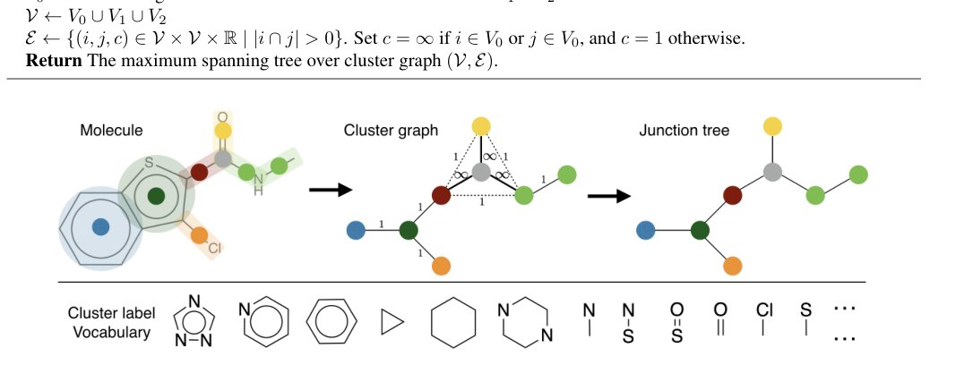
Figure 9: Illustration of tree decomposition and sample of cluster label vocabulary.
图 9:树分解示意以及簇标号词表的样本。
Appendix B Stereochemistry
附录 B 立体化学
Though usually presented as two-dimensional graphs, molecules are three-dimensional objects, i.e. molecules are defined not only by its atom types and bond connections, but also the spatial configuration between atoms (chiral atoms and cis-trans isomerism). Stereoisomers are molecules that have the same 2D structure, but differ in the 3D orientations of their atoms in space. We note that stereochemical feasibility could not be simply encoded as context free or attribute grammars.
尽管通常被画成二维图,分子其实是三维对象,也就是说分子不仅由原子类型和键连接定义,还由原子之间的空间构型定义(手性原子和顺反异构)。立体异构体是具有相同二维结构、但原子在空间中的三维取向不同的分子。我们指出,立体化学可行性并不能简单地编码成上下文无关文法或属性文法。
Empirically, we found it more efficient to predict the stereochemical configuration separately from the molecule generation. Specifically, the JT-VAE first generates the 2D structure of a molecule , following the same procedure described in section 2. Then we generate all its stereoisomers using RDKit’s EnumerateStereoisomers function, which identifies atoms that could be chiral. For each isomer , we encode its graph representation with the graph encoder and compute their cosine similarity (note that is stochastic). We reconstruct the final 3D structure by picking the stereoisomer . Since on average only few atoms could have stereochemical variations, this post ranking process is very efficient. Combining this with tree and graph generation, the molecule reconstruction loss becomes
经验上,我们发现把立体化学构型的预测与分子生成分开更为高效。具体来说,JT-VAE 先按第 2 节描述的同一流程生成分子 的二维结构。然后我们用 RDKit 的 EnumerateStereoisomers 函数生成它的全部立体异构体 ,该函数会识别可能手性的原子。对每个异构体 ,我们用图编码器编码其图表示 ,并计算余弦相似度 (注意 是随机的)。我们通过选取立体异构体 来重建最终的三维结构。由于平均只有少数原子可能有立体化学变化,这一事后排序过程非常高效。把它与树生成和图生成结合起来,分子重建损失 变为
Appendix C Training Details
附录 C 训练细节
By applying tree decomposition over 240K molecules in ZINC dataset, we collected our vocabulary set of size . The hidden state dimension is 450 for all modules in JT-VAE and the latent bottleneck dimension is 56. For the graph encoder, the initial atom features include its atom type, degree, its formal charge and its chiral configuration. Bond feature is a concatenation of its bond type, whether the bond is in a ring, and its cis-trans configuration. For our tree encoder, we represent each cluster with a neural embedding vector, similar to word embedding for words. The tree and graph decoder use the same feature setting as encoders. The graph encoder and decoder runs three iterations of neural message passing. For fair comparison to SMILES based method, we minimized feature engineering. We use PyTorch to implement all neural components and RDKit to process molecules.
通过对 ZINC 数据集中的 24 万个分子做树分解,我们收集到规模为 的词表 。JT-VAE 中所有模块的隐状态维数为 450,潜瓶颈维数为 56。对图编码器,初始原子特征包括原子类型、度数、形式电荷和手性构型。键特征是其键类型、该键是否在环中、以及顺反构型的拼接。对树编码器,我们用神经嵌入向量表示每个簇,类似于词的词嵌入。树解码器和图解码器使用与编码器相同的特征设置。图编码器和解码器各运行三轮神经消息传递。为与基于 SMILES 的方法公平比较,我们尽量减少特征工程。我们用 PyTorch 实现全部神经组件,用 RDKit 处理分子。
Appendix D More Experimental Results
附录 D 更多实验结果
Sampled Molecules Note that a degenerate model could also achieve 100% prior validity by keep generating simple structures like chains. To prove that our model does not converge to such trivial solutions, we randomly sample and plot 250 molecules from prior distribution . As shown in Figure 10, our sampled molecules present rich variety and structural complexity. This demonstrates the soundness of the prior validity improvement of our model.
采样分子 注意,一个退化模型也可以通过不断生成简单结构(例如链)达到 100% 的先验有效性。为证明我们的模型没有收敛到这类平凡解,我们从先验分布 随机采样并画出 250 个分子。如图 10 所示,采样出的分子呈现丰富的多样性和结构复杂度。这表明我们模型在先验有效性上的改善是扎实的。
Neighborhood Visualization Given a molecule, we follow Kusner et al. 2017 to construct a grid visualization of its neighborhood. Specifically, we encode a molecule into the latent space and generate two random orthogonal unit vectors as two axis of a grid. Moving in combinations of these directions yields a set of latent vectors and we decode them into corresponding molecules. In Figure 11 and 12, we visualize the local neighborhood of two molecules presented in Dai et al. 2018. Figure 11 visualizes the same molecule in Figure 6, but with wider neighborhood ranges.
邻域可视化 给定一个分子,我们按 Kusner 等(2017)构造其邻域的网格可视化。具体来说,我们把分子编码到潜空间,并生成两个随机正交单位向量作为网格的两个轴。沿这些方向的组合移动得到一组潜向量,我们再把它们解码成对应分子。图 11 和图 12 可视化了 Dai 等(2018)中给出的两个分子的局部邻域。图 11 可视化的是与图 6 相同的分子,但邻域范围更宽。
Bayesian Optimization We directly used open sourced implementation in Kusner et al. 2017 for Bayesian optimization (BO). Specifically, we train a sparse Gaussian process with 500 inducing points to predict properties of molecules. Five iterations of batch BO with expected improvement heuristic is used to propose new latent vectors. In each iteration, 50 latent vectors are proposed, from which molecules are decoded and added to the training set for next iteration. We perform 10 independent runs and aggregate results. In Figure 13, we present the top 50 molecules found among 10 runs using JT-VAE. Following Kusner et al. 2017’s implementation, the scores reported are normalized to zero mean and unit variance by the mean and variance computed from training set.
贝叶斯优化 我们直接使用 Kusner 等(2017)开源的贝叶斯优化(BO)实现。具体来说,我们训练带 500 个诱导点的稀疏高斯过程来预测分子性质。用期望改进启发式做五轮批量 BO 以提出新的潜向量。每一轮提出 50 个潜向量,从中解码出分子并加入下一轮的训练集。我们做 10 次独立运行并汇总结果。图 13 给出用 JT-VAE 在 10 次运行中找到的最好的 50 个分子。按 Kusner 等(2017)的实现,所报告的分数用训练集算出的均值和方差归一化到零均值、单位方差。
Constrained Optimization For this task, a property predictor is trained jointly with VAE to predict from the latent embedding of . is a feed-forward network with one hidden layer of dimension 450 followed by activation. To optimize a molecule , we start with its mean encoding and apply 80 gradient ascent steps: with . 80 molecules are decoded from latent vectors and their property is calculated. Molecular similarity is calculated via Morgan fingerprint of radius 2 with Tanimoto similarity. For each molecule , we report the best modified molecule with for some threshold . In Figure 14, we present three groups of modification examples with . For each group, we present top three pairs that leads to best improvement as well as one pair decreased property (). This is caused by inaccurate property prediction. From Figure 14, we can see that tighter similarity constraint forces the model to preserve the original structure.
带约束的优化 对这一任务,性质预测器 与 VAE 联合训练,从 的潜嵌入预测 。 是带一个 450 维隐层再接 激活的前馈网络。为优化分子 ,我们从其均值编码 出发,做 80 步梯度上升:,其中 。从潜向量 解码出 80 个分子并计算其性质。分子相似度 通过半径为 2 的 Morgan 指纹与 Tanimoto 相似度计算。对每个分子 ,我们报告在某个阈值 下满足 的最好修改分子 。图 14 给出 三组修改例子。对每一组,我们展示带来最好改善 的前三对,以及一对性质下降的例子()。这是由不准确的性质预测造成的。从图 14 可以看出,更紧的相似度约束迫使模型保留原来的结构。
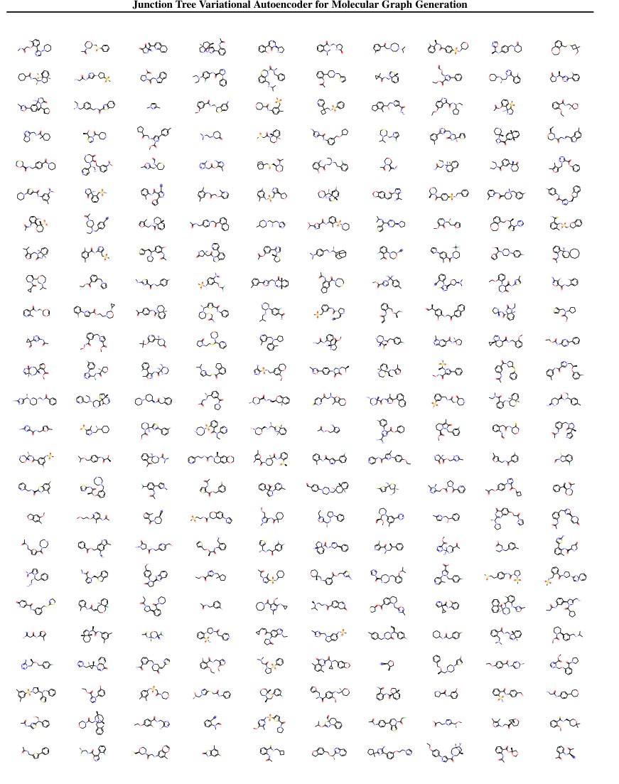
Figure 10: 250 molecules sampled from prior distribution .
图 10:从先验分布 采样的 250 个分子。
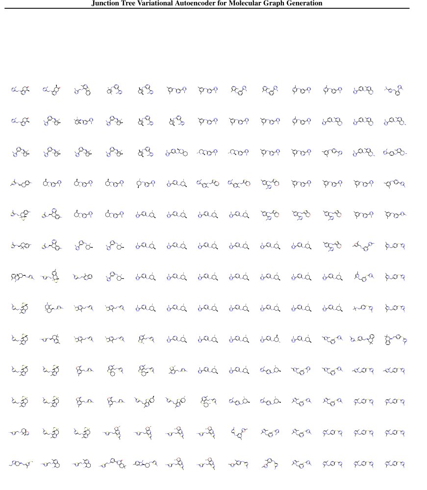
Figure 11: Neighborhood visualization of molecule C[C@H]1CC(Nc2cncc(-c3nncn3C)c2)CC@HC1.
图 11:分子 C[C@H]1CC(Nc2cncc(-c3nncn3C)c2)CC@HC1 的邻域可视化。
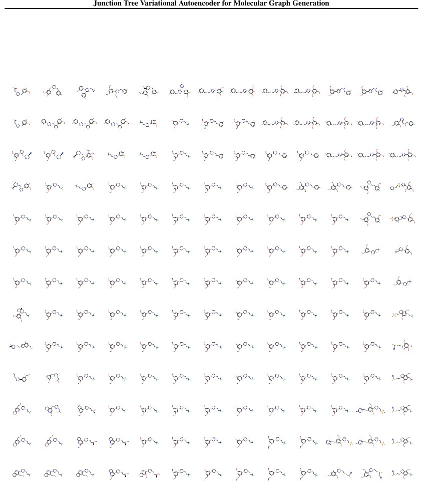
Figure 12: Neighborhood visualization of molecule COc1cc(OC)cc([C@H]2CCNH+C2)c1.
图 12:分子 COc1cc(OC)cc([C@H]2CCNH+C2)c1 的邻域可视化。
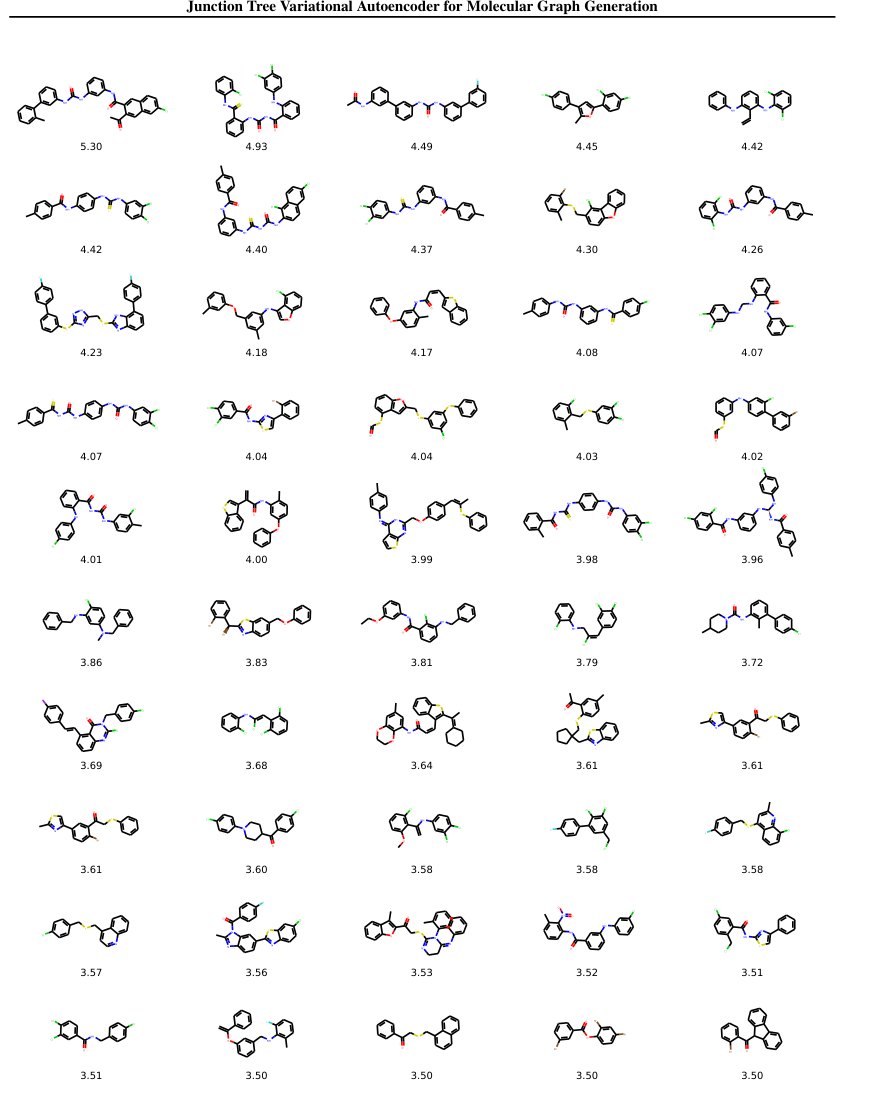
Figure 13: Top 50 molecules found by Bayesian optimization using JT-VAE.
图 13:用 JT-VAE 经贝叶斯优化找到的最好的 50 个分子。
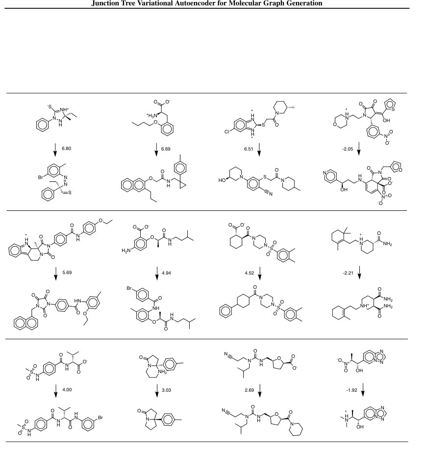
Figure 14: Row 1-3: Molecule modification results with similarity constraint . For each group, we plot the top three pairs that leads to actual property improvement, and one pair with decreased property. We can see that tighter similarity constraint forces the model to preserve the original structure.
图 14:第 1–3 行:相似度约束 下的分子修改结果。对每一组,我们画出带来实际性质改善的前三对,以及一对性质下降的例子。可以看出,更紧的相似度约束迫使模型保留原来的结构。