Offline Reinforcement Learning with Implicit Q-Learning

用隐式 Q 学习做离线强化学习

Ilya Kostrikov    Ashvin Nair & Sergey Levine Affiliation: Department of Electrical Engineering and Computer Science Affiliation: University of California, Berkeley Affiliation: {kostrikov,anair17}@berkeley.edu , svlevine@eecs.berkeley.edu

Abstract

摘要

Offline reinforcement learning requires reconciling two conflicting aims: learning a policy that improves over the behavior policy that collected the dataset, while at the same time minimizing the deviation from the behavior policy so as to avoid errors due to distributional shift. This trade-off is critical, because most current offline reinforcement learning methods need to query the value of unseen actions during training to improve the policy, and therefore need to either constrain these actions to be in-distribution, or else regularize their values. We propose a new offline RL method that never needs to evaluate actions outside of the dataset, but still enables the learned policy to improve substantially over the best behavior in the data through generalization. The main insight in our work is that, instead of evaluating unseen actions from the latest policy, we can approximate the policy improvement step implicitly by treating the state value function as a random variable, with randomness determined by the action (while still integrating over the dynamics to avoid excessive optimism), and then taking a state conditional upper expectile of this random variable to estimate the value of the best actions in that state. This leverages the generalization capacity of the function approximator to estimate the value of the best available action at a given state without ever directly querying a Q-function with this unseen action. Our algorithm alternates between fitting this upper expectile value function and backing it up into a Q-function, without any explicit policy. Then, we extract the policy via advantage-weighted behavioral cloning, which also avoids querying out-of-sample actions. We dub our method implicit Q-learning (IQL). IQL is easy to implement, computationally efficient, and only requires fitting an additional critic with an asymmetric L2 loss.[^1] IQL demonstrates the state-of-the-art performance on D4RL, a standard benchmark for offline reinforcement learning. We also demonstrate that IQL achieves strong performance fine-tuning using online interaction after offline initialization.

离线强化学习需要调和两个互相冲突的目标：既要学出比采集数据的行为策略更好的策略，又要尽量少偏离行为策略，以免分布偏移带来误差。这一权衡很关键——多数现有离线 RL 方法在训练时都要查询未见动作的价值，才能改进策略，因此要么把这些动作约束在分布内，要么对其价值做正则。我们提出一种离线 RL 方法：训练过程中从不评估数据集之外的动作，却仍能通过泛化，使学到的策略显著超过数据中最好的行为。核心洞见是：不必用最新策略去评估未见动作，而是把状态价值函数看成随机变量（随机性来自动作；同时对动力学求期望以免过度乐观），再取该随机变量在状态下的上侧 expectile，去估计该状态下最好动作的价值。这样借助函数逼近器的泛化能力估计「给定状态下最好可用动作」的价值，却从不直接用这个未见动作去查询 Q 函数。算法在拟合该上侧 expectile 价值函数、再把它备份进 Q 函数之间交替，全程不显式引入策略；随后用优势加权行为克隆抽取策略，同样避免查询样本外动作。我们称该方法为隐式 Q 学习（IQL）。IQL 易于实现、计算高效，只需再用一个非对称 L2 损失拟合额外的 critic。[^1] 在离线 RL 标准基准 D4RL 上，IQL 达到当时最优表现；我们还表明，离线初始化之后再用在线交互微调，IQL 同样很强。

1 Introduction

1 引言

Offline reinforcement learning (RL) addresses the problem of learning effective policies entirely from previously collected data, without online interaction (Fujimoto et al. 2019; Lange et al. 2012). This is very appealing in a range of real-world domains, from robotics to logistics and operations research, where real-world exploration with untrained policies is costly or dangerous, but prior data is available. However, this also carries with it major challenges: improving the policy beyond the level of the behavior policy that collected the data requires estimating values for actions other than those that were seen in the dataset, and this, in turn, requires trading off policy improvement against distributional shift, since the values of actions that are too different from those in the data are unlikely to be estimated accurately. Prior methods generally address this by either constraining the policy to limit how far it deviates from the behavior policy (Fujimoto et al. 2019; Wu et al. 2019; Fujimoto & Gu 2021; Kumar et al. 2019; Nair et al. 2020; Wang et al. 2020), or by regularizing the learned value functions to assign low values to out-of-distribution actions (Kumar et al. 2020; Kostrikov et al. 2021). Nevertheless, this imposes a trade-off between how much the policy improves and how vulnerable it is to misestimation due to distributional shift. Can we devise an offline RL method that avoids this issue by never needing to directly query or estimate values for actions that were not seen in the data?

离线强化学习（RL）要解决的是：完全依赖事先采集的数据学习有效策略，不做在线交互（Fujimoto et al. 2019；Lange et al. 2012）。从机器人到物流与运筹，许多真实场景里，用未训练好的策略去探索代价高昂或危险，但历史数据往往现成，因此离线设定很有吸引力。挑战同样尖锐：要把策略推到行为策略之上，就必须估计数据中未见过的动作的价值；而这又要求在「改进策略」与「分布偏移」之间权衡——偏离数据太远的动作，价值很难估准。先前方法通常要么约束策略，限制它相对行为策略偏离多远（Fujimoto et al. 2019；Wu et al. 2019；Fujimoto & Gu 2021；Kumar et al. 2019；Nair et al. 2020；Wang et al. 2020），要么正则学到的价值函数，让分布外动作拿低分（Kumar et al. 2020；Kostrikov et al. 2021）。这仍是在「改进多少」与「因分布偏移而误估的风险」之间做折中。能否设计一种离线 RL 方法，直接避免查询或估计数据中未见动作的价值？

In this work, we start from an observation that in-distribution constraints widely used in prior work might not be sufficient to avoid value function extrapolation, and we ask whether it is possible to learn an optimal policy with in-sample learning, without ever querying the values of any unseen actions. The key idea in our method is to approximate an upper expectile of the distribution over values with respect to the distribution of dataset actions for each state. We alternate between fitting this value function with expectile regression, and then using it to compute Bellman backups for training the $Q$-function. We show that we can do this simply by modifying the loss function in a SARSA-style TD backup, without ever using out-of-sample actions in the target value. Once this $Q$-function has converged, we extract the corresponding policy using advantage-weighted behavioral cloning. This approach does not require explicit constraints or explicit regularization of out-of-distribution actions during value function training, though our policy extraction step does implicitly enforce a constraint, as discussed in prior work on advantage-weighted regression (Peters & Schaal 2007; Peng et al. 2019; Nair et al. 2020; Wang et al. 2020).

本文从一点观察出发：先前广泛使用的分布内约束，未必足以避免价值函数外推；我们追问：能否用样本内学习学到最优策略，从不查询任何未见动作的价值。方法的关键是：对每个状态，近似「相对数据集动作分布」的价值分布上侧 expectile。我们交替用 expectile 回归拟合该价值函数，再用它计算训练 $Q$ 函数的 Bellman 备份。只需改 SARSA 风格 TD 备份的损失函数即可完成，目标价值中从不使用样本外动作。$Q$ 函数收敛后，再用优势加权行为克隆抽取对应策略。价值函数训练阶段不需要显式约束或对分布外动作做显式正则；策略抽取步会隐式施加约束，这与优势加权回归的既有讨论一致（Peters & Schaal 2007；Peng et al. 2019；Nair et al. 2020；Wang et al. 2020）。

Our main contribution is implicit Q-learning (IQL), a new offline RL algorithm that avoids ever querying values of unseen actions while still being able to perform multi-step dynamic programming updates. Our method is easy to implement by making a small change to the loss function in a simple SARSA-like TD update and is computationally very efficient. Furthermore, our approach demonstrates the state-of-the-art performance on D4RL, a popular benchmark for offline reinforcement learning. In particular, our approach significantly improves over the prior state-of-the-art on challenging Ant Maze tasks that require to “stitch” several sub-optimal trajectories. Finally, we demonstrate that our approach is suitable for finetuning; after initialization from offline RL, IQL is capable of improving policy performance utilizing additional interactions.

本文主要贡献是隐式 Q 学习（IQL）：一种离线 RL 算法，从不查询未见动作的价值，却仍能做多步动态规划更新。实现上只需对简单的类 SARSA TD 更新改一点损失，计算也很高效。此外，IQL 在流行离线基准 D4RL 上达到当时最优；尤其在需要把若干次优轨迹「缝合」起来的困难 Ant Maze 任务上，相对先前最优有显著提升。我们还表明该方法适于微调：离线 RL 初始化之后，IQL 能利用额外交互继续提升策略表现。

2 Related work

2 相关工作

A significant portion of recently proposed offline RL methods are based on either constrained or regularized approximate dynamic programming (e.g., Q-learning or actor-critic methods), with the constraint or regularizer serving to limit deviation from the behavior policy. We will refer to these methods as “multi-step dynamic programming” algorithms, since they perform true dynamic programming for multiple iterations, and therefore can in principle recover the optimal policy if provided with high-coverage data. The constraints can be implemented via an explicit density model (Wu et al. 2019; Fujimoto et al. 2019; Kumar et al. 2019), implicit divergence constraints (Nair et al. 2020; Wang et al. 2020; Peters & Schaal 2007; Peng et al. 2019), or by adding a supervised learning term to the policy improvement objective (Fujimoto & Gu 2021). Several works have also proposed to directly regularize the Q-function to produce low values for out-of-distribution actions (Kostrikov et al. 2021; Kumar et al. 2020). Our method is also a multi-step dynamic programming algorithm. However, in contrast to prior works, our method completely avoids directly querying the learned Q-function with unseen actions during training, removing the need for any constraint during this stage, though the subsequent policy extraction, which is based on advantage-weighted regression (Peng et al. 2019; Nair et al. 2020), does apply an implicit constraint. However, this policy does not actually influence value function training.

近年来大量离线 RL 方法建立在带约束或正则的近似动态规划之上（如 Q-learning 或 actor-critic），约束或正则用来限制相对行为策略的偏离。我们称这类为「多步动态规划」算法：它们真正做多轮动态规划，数据覆盖充分时原则上可恢复最优策略。约束可通过显式密度模型（Wu et al. 2019；Fujimoto et al. 2019；Kumar et al. 2019）、隐式散度约束（Nair et al. 2020；Wang et al. 2020；Peters & Schaal 2007；Peng et al. 2019），或在策略改进目标上加监督学习项（Fujimoto & Gu 2021）实现。也有工作直接正则 $Q$ 函数，使分布外动作得到低价值（Kostrikov et al. 2021；Kumar et al. 2020）。我们的方法同样是多步动态规划算法；与先前工作不同的是，训练时完全避免用未见动作直接查询学到的 $Q$ 函数，因而该阶段无需任何约束——尽管后续基于优势加权回归（Peng et al. 2019；Nair et al. 2020）的策略抽取会施加隐式约束，且该策略并不影响价值函数训练。

In contrast to multi-step dynamic programming methods, several recent works have proposed methods that rely either on a single step of policy iteration, fitting the value function or Q-function of the behavior policy and then extracting the corresponding greedy policy (Peng et al. 2019; Brandfonbrener et al. 2021), or else avoid value functions completely and utilize behavioral cloning-style objectives (Chen et al. 2021). We collectively refer to these as “single-step” approaches. These methods avoid needing to query unseen actions as well, since they either use no value function at all, or learn the value function of the behavior policy. Although these methods are simple to implement and effective on the MuJoCo locomotion tasks in D4RL, we show that such single-step methods perform very poorly on more complex datasets in D4RL, which require combining parts of suboptimal trajectories (“stitching”). Prior multi-step dynamic programming methods perform much better in such settings, as does our method. We discuss this distinction in more detail in Section 5.1. Our method also shares the simplicity and computational efficiency of single-step approaches, providing an appealing combination of the strengths of both types of methods.

与多步动态规划相对，若干近期工作依赖单步策略迭代——拟合行为策略的价值或 $Q$ 函数再抽取贪婪策略（Peng et al. 2019；Brandfonbrener et al. 2021）——或完全不用价值函数、采用行为克隆式目标（Chen et al. 2021）。我们统称其为「单步」方法。它们同样避免查询未见动作：要么没有价值函数，要么只学行为策略的价值。这类方法实现简单，在 D4RL 的 MuJoCo 运动任务上有效；但我们表明，在需要把次优轨迹片段「缝合」起来的更复杂 D4RL 数据上，单步方法表现很差。先前多步动态规划方法在这些设定下好得多，我们的方法也是。第 5.1 节再细谈这一区别。我们的方法还保有单步方法的简洁与计算效率，因而兼取两类方法之长。

Our method is based on estimating the characteristics of a random variable. Several recent works involve approximating statistical quantities of the value function distribution. In particular, quantile regression (Koenker & Hallock 2001) has been previously used in reinforcement learning to estimate the quantile function of a state-action value function (Dabney et al. 2018b; Dabney et al. 2018a; Kuznetsov et al. 2020). Although our method is related, in that we perform expectile regression, our aim is not to estimate the distribution of values that results from stochastic transitions, but rather estimate expectiles of the state value function with respect to random actions. This is a very different statistic: our aim is not to determine how the $Q$-value can vary with different future outcomes, but how the $Q$-value can vary with different actions while averaging together future outcomes due to stochastic dynamics. While prior work on distributional RL can also be used for offline RL, it would suffer from the same action extrapolation issues as other methods, and would require similar constraints or regularization, while our method does not.

我们的方法基于估计随机变量的特征。若干近期工作近似价值函数分布的统计量；尤其分位数回归（Koenker & Hallock 2001）已被用于强化学习，以估计状态–动作价值函数的分位函数（Dabney et al. 2018b；Dabney et al. 2018a；Kuznetsov et al. 2020）。我们虽相关——做的是 expectile 回归——但目标不是估计随机转移带来的价值分布，而是相对随机动作估计状态价值函数的 expectile。这是很不同的统计量：我们关心的不是未来结果如何让 $Q$ 值变化，而是在对不同动作变化时，$Q$ 值如何变化——同时对随机动力学的未来结果取平均。先前分布强化学习也可用于离线 RL，但仍会遇到其他方法同样的动作外推问题，需要类似约束或正则；我们的方法不需要。

3 Preliminaries

3 预备知识

The RL problem is formulated in the context of a Markov decision process (MDP) $(\mathcal{S},\mathcal{A},p_{0}(s),p(s^{\prime}|s,a),r(s,a),\gamma)$, where $\mathcal{S}$ is a state space, $\mathcal{A}$ is an action space, $p_{0}(s)$ is a distribution of initial states, $p(s^{\prime}|s,a)$ is the environment dynamics, $r(s,a)$ is a reward function, and $\gamma$ is a discount factor. The agent interacts with the MDP according to a policy $\pi(a|s)$. The goal is to obtain a policy that maximizes the cumulative discounted returns:

强化学习问题在马尔可夫决策过程（MDP）$(\mathcal{S},\mathcal{A},p_{0}(s),p(s^{\prime}|s,a),r(s,a),\gamma)$ 中表述：其中 $\mathcal{S}$ 为状态空间，$\mathcal{A}$ 为动作空间，$p_{0}(s)$ 为初始状态分布，$p(s^{\prime}|s,a)$ 为环境动力学，$r(s,a)$ 为奖励函数，$\gamma$ 为折扣因子。智能体按策略 $\pi(a|s)$ 与 MDP 交互，目标是最大化累积折扣回报：

$$\pi^{*}=\argmax_{\pi}\mathbb{E}_{\pi}\left[\sum_{t=0}^{\infty}\gamma^{t}r(s_{t},a_{t})|\allowbreak s_{0}\sim p_{0}(\cdot),\allowbreak a_{t}\sim\pi(\cdot|s_{t}),\allowbreak s_{t+1}\sim p(\cdot|s_{t},a_{t})\right].$$

Off-policy RL methods based on approximate dynamic programming typically utilize a state-action value function ($Q$-function), referred to as $Q(s,a)$, which corresponds to the discounted returns obtained by starting from the state $s$ and action $a$, and then following the policy $\pi$.

基于近似动态规划的离策略 RL 方法通常使用状态–动作价值函数（$Q$ 函数）$Q(s,a)$：从状态 $s$、动作 $a$ 出发再遵循策略 $\pi$ 所得的折扣回报。

Offline reinforcement learning.

In contrast to online (on-policy or off-policy) RL methods, offline RL uses previously collected data without any additional data collection. Like many recent offline RL methods, our work builds on approximate dynamic programming methods that minimize temporal difference error, according to the following loss:

离线强化学习。

与在线（同策略或离策略）RL 不同，离线 RL 只用事先采集的数据，不再额外采集。与许多近期离线 RL 方法一样，我们建立在最小化时序差分误差的近似动态规划之上，损失如下：

$$L_{TD}(\theta)=\mathbb{E}_{(s,a,s^{\prime})\sim\mathcal{D}}[(r(s,a)+\gamma\max_{a^{\prime}}Q_{\hat{\theta}}(s^{\prime},a^{\prime})-Q_{\theta}(s,a))^{2}], \tag{1}$$

where $\mathcal{D}$ is the dataset, $Q_{\theta}(s,a)$ is a parameterized Q-function, $Q_{\hat{\theta}}(s,a)$ is a target network (e.g., with soft parameters updates defined via Polyak averaging), and the policy is defined as $\pi(s)=\argmax_{a}Q_{\theta}(s,a)$. Most recent offline RL methods modify either the value function loss (above) to regularize the value function in a way that keeps the resulting policy close to the data, or constrain the $\argmax$ policy directly. This is important because out-of-distribution actions $a^{\prime}$ can produce erroneous values for $Q_{\hat{\theta}}(s^{\prime},a^{\prime})$ in the above objective, often leading to overestimation as the policy is defined to maximize the (estimated) Q-value.

其中 $\mathcal{D}$ 为数据集，$Q_{\theta}(s,a)$ 为参数化 $Q$ 函数，$Q_{\hat{\theta}}(s,a)$ 为目标网络（例如经 Polyak 平均做软更新），策略定义为 $\pi(s)=\argmax_{a}Q_{\theta}(s,a)$。多数近期离线 RL 方法要么改价值函数损失（如上）以正则价值、使所得策略贴近数据，要么直接约束 $\argmax$ 策略。这很重要：分布外动作 $a^{\prime}$ 会在上述目标中给 $Q_{\hat{\theta}}(s^{\prime},a^{\prime})$ 带来错误价值，又因策略定义为最大化（估计的）$Q$ 值，常导致高估。

4 Implicit Q-Learning

4 隐式 Q 学习

In this work, we aim to entirely avoid querying out-of-sample (unseen) actions in our TD loss. We start by considering fitted $Q$ evaluation with a SARSA-style objective, which simply aims to learn the value of the dataset policy $\pi_{\beta}$ (also called the behavior policy):

本文希望在 TD 损失中完全避免查询样本外（未见）动作。我们先考虑用类 SARSA 目标做拟合 $Q$ 评估，其目的只是学习数据集策略 $\pi_{\beta}$（也称行为策略）的价值：

$$L(\theta)=\mathbb{E}_{(s,a,s^{\prime},a^{\prime})\sim\mathcal{D}}[(r(s,a)+\gamma Q_{\hat{\theta}}(s^{\prime},a^{\prime})-Q_{\theta}(s,a))^{2}]. \tag{2}$$

This objective never queries values for out-of-sample actions, in contrast to Equation 1. One specific property of this objective that is important for this work is that it uses mean squared error (MSE) that fits $Q_{\theta}(s,a)$ to predict the mean statistics of the TD targets. Thus, if we assume unlimited capacity and no sampling error, the optimal parameters should satisfy

与公式 1 不同，该目标从不查询样本外动作的价值。对本工作很关键的一点是：它用均方误差（MSE）拟合 $Q_{\theta}(s,a)$，去预测 TD 目标的均值统计量。因此，若假设容量无限且无采样误差，最优参数应满足

$$Q_{\theta^{*}}(s,a)\approx r(s,a)+\gamma\mathbb{E}{\begin{subarray}{c}s^{\prime}\sim p(\cdot|s,a)\
a^{\prime}\sim\pi{\beta}(\cdot|s)\end{subarray}}[Q_{\hat{\theta}}(s^{\prime},a^{\prime})]. \tag{3}$$

$$Q_{\theta^{*}}(s,a)\approx r(s,a)+\gamma\mathbb{E}_{\begin{subarray}{c}s^{\prime}\sim p(\cdot|s,a)\\ a^{\prime}\sim\pi_{\beta}(\cdot|s)\end{subarray}}[Q_{\hat{\theta}}(s^{\prime},a^{\prime})]. \tag{3}$$

Prior work (Brandfonbrener et al. 2021; Peng et al. 2019) has proposed directly using this objective to learn $Q^{\pi_{\beta}}$, and then train the policy $\pi_{\psi}$ to maximize $Q^{\pi_{\beta}}$. This avoids any issues with out-of-distribution actions, since the TD loss only uses dataset actions. However, while this procedure works well empirically on simple MuJoCo locomotion tasks in D4RL, we will show that it performs very poorly on more complex tasks that benefit from multi-step dynamic programming. In our method, which we derive next, we retain the benefits of using this SARSA-like objective, but modify it so that it allows us to perform multi-step dynamic programming and learn a near-optimal Q-function.

先前工作（Brandfonbrener et al. 2021；Peng et al. 2019）提出直接用该目标学 $Q^{\pi_{\beta}}$，再训练策略 $\pi_{\psi}$ 最大化 $Q^{\pi_{\beta}}$。TD 损失只用数据集动作，因而避开分布外动作问题。该流程在 D4RL 简单 MuJoCo 运动任务上经验表现不错，但我们会表明：在更受益于多步动态规划的复杂任务上，它表现很差。接下来推导的方法保留这类 SARSA 目标的优点，同时加以改造，使之能做多步动态规划并学到近最优 $Q$ 函数。

Our method will perform a $Q$-function update similar to Equation 2, but we will aim to estimate the maximum $Q$-value over actions that are in the support of the data distribution. Crucially, we will show that it is possible to do this without ever querying the learned Q-function on out-of-sample actions by utilizing expectile regression. Formally, the value function we aim to learn is given by:

我们的方法将做与公式 2 类似的 $Q$ 更新，但目标是估计数据分布支撑上动作的最大 $Q$ 值。关键是：我们表明可以从不在样本外动作上查询学到的 $Q$ 函数，借助 expectile 回归做到这一点。形式上，要学的价值函数由下式给出：

$$L(\theta)=\mathbb{E}{(s,a,s^{\prime})\sim\mathcal{D}}[(r(s,a)+\gamma\max{\begin{subarray}{c}a^{\prime}\in\mathcal{A}\
\text{s.t. }\pi_{\beta}(a^{\prime}|s^{\prime})>0\end{subarray}}Q_{\hat{\theta}}(s^{\prime},a^{\prime})-Q_{\theta}(s,a))^{2}]. \tag{4}$$

$$L(\theta)=\mathbb{E}_{(s,a,s^{\prime})\sim\mathcal{D}}[(r(s,a)+\gamma\max_{\begin{subarray}{c}a^{\prime}\in\mathcal{A}\\ \text{s.t. }\pi_{\beta}(a^{\prime}|s^{\prime})>0\end{subarray}}Q_{\hat{\theta}}(s^{\prime},a^{\prime})-Q_{\theta}(s,a))^{2}]. \tag{4}$$

Our algorithm, implicit Q-Learning (IQL), aims to estimate this objective while evaluating the $Q$-function only on the state-action pairs in the dataset. To this end, we propose to fit $Q_{\theta}(s,a)$ to estimate state-conditional expectiles of the target values, and show that specific expectiles approximate the maximization defined above. In Section 4.4 we show that this approach performs multi-step dynamic programming in theory, and in Section 5.1 we show that it does so in practice.

算法隐式 Q 学习（IQL）要在只对数据集中状态–动作对评估 $Q$ 的前提下估计该目标。为此，我们提出用 $Q_{\theta}(s,a)$ 估计目标价值的状态条件 expectile，并表明特定 expectile 可近似上述最大化。第 4.4 节从理论上说明该方法做多步动态规划；第 5.1 节从实验上说明它确实如此。

4.1 Expectile Regression

4.1 Expectile 回归

Practical methods for estimating various statistics of a random variable have been thoroughly studies in applied statistics and econometrics. The $\tau\in(0,1)$ expectile of some random variable $X$ is defined as a solution to the asymmetric least squares problem:

估计随机变量各类统计量的实用方法，在应用统计与计量经济学中已有充分研究。随机变量 $X$ 的 $\tau\in(0,1)$ expectile 定义为非对称最小二乘问题的解：

$$\argmin_{m_{\tau}}\mathbb{E}_{x\sim X}[L_{2}^{\tau}(x-m_{\tau})],$$

where $L_{2}^{\tau}(u)=|\tau-\mathbbm{1}(u<0)|u^{2}$.

其中 $L_{2}^{\tau}(u)=|\tau-\mathbbm{1}(u<0)|u^{2}$。

That is, for $\tau>0.5$, this asymmetric loss function downweights the contributions of $x$ values smaller than $m_{\tau}$ while giving more weights to larger values (see Figure 1, left). Expectile regression is closely related to quantile regression (Koenker & Hallock 2001), which is a popular technique for estimating quantiles of a distribution widely used in reinforcement learning (Dabney et al. 2018b; Dabney et al. 2018a) [^2]. The quantile regression loss is defined as an asymmetric $\ell_{1}$ loss.

亦即，当 $\tau>0.5$ 时，该非对称损失会降低小于 $m_{\tau}$ 的 $x$ 的贡献，同时给更大的值更高权重（见图 1 左）。Expectile 回归与分位数回归（Koenker & Hallock 2001）密切相关；后者是估计分布分位数的常用技术，在强化学习中被广泛使用（Dabney et al. 2018b；Dabney et al. 2018a）[^2]。分位数回归损失定义为非对称 $\ell_{1}$ 损失。

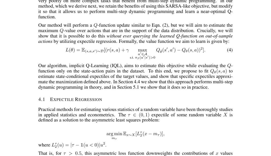
Figure 1: Left: The asymmetric squared loss used for expectile regression. $\tau=0.5$ corresponds to the standard mean squared error loss, while $\tau=0.9$ gives more weight to positives differences. Center: Expectiles of a normal distribution. Right: an example of estimating state conditional expectiles of a two-dimensional random variable. Each $x$ corresponds to a distribution over $y$. We can approximate a maximum of this random variable with expectile regression: $\tau=0.5$ correspond to the conditional mean statistics of the distribution, while $\tau\approx 1$ approximates the maximum operator over in-support values of $y$.

图 1：左： expectile 回归所用的非对称平方损失。$\tau=0.5$ 对应标准均方误差；$\tau=0.9$ 对正残差赋予更大权重。中： 正态分布的 expectile。右： 估计二维随机变量状态条件 expectile 的例子。每个 $x$ 对应 $y$ 上的一个分布。可用 expectile 回归近似该随机变量的最大值：$\tau=0.5$ 对应条件均值，$\tau\approx 1$ 则近似对支撑内 $y$ 的最大化算子。

We can also use this formulation to predict expectiles of a conditional distribution:

也可用该形式预测条件分布的 expectile：

$$\argmin_{m_{\tau}(x)}\mathbb{E}_{(x,y)\sim\mathcal{D}}[L_{2}^{\tau}(y-m_{\tau}(x))].$$

Figure 1 (right) illustrates conditional expectile regression on a simple two-dimensional distribution. Note that we can optimize this objective with stochastic gradient descent. It provides unbiased gradients and is easy to implement with standard machine learning libraries.

图 1（右）展示了在简单二维分布上做条件 expectile 回归。注意该目标可用随机梯度下降优化，梯度无偏，且易于用标准机器学习库实现。

4.2 Learning the Value Function with Expectile Regression

4.2 用 Expectile 回归学习价值函数

Expectile regression provides us with a powerful framework to estimate statistics of a random variable beyond mean regression. We can use expectile regression to modify the policy evaluation objective in Equation 2 to predict an upper expectile of the TD targets that approximates the maximum of $r(s,a)+\gamma Q_{\hat{\theta}}(s^{\prime},a^{\prime})$ over actions $a^{\prime}$ constrained to the dataset actions, as in Equation 4. This leads to the following expectile regression objective:

Expectile 回归提供了在均值回归之外估计随机变量统计量的有力框架。我们可用它改写公式 2 中的策略评估目标，去预测 TD 目标的上侧 expectile，从而近似公式 4 中在数据集动作约束下对 $r(s,a)+\gamma Q_{\hat{\theta}}(s^{\prime},a^{\prime})$ 关于 $a^{\prime}$ 的最大化。由此得到如下 expectile 回归目标：

$$\displaystyle L(\theta)=\mathbb{E}_{(s,a,s^{\prime},a^{\prime})\sim\mathcal{D}}[L_{2}^{\tau}(r(s,a)+\gamma Q_{\hat{\theta}}(s^{\prime},a^{\prime})-Q_{\theta}(s,a))].$$

However, this formulation has a significant drawback. Instead of estimating expectiles just with respect to the actions in the support of the data, it also incorporates stochasticity that comes from the environment dynamics $s^{\prime}\sim p(\cdot|s,a)$. Therefore, a large target value might not necessarily reflect the existence of a single action that achieves that value, but rather a “lucky” sample that happened to have transitioned into a good state. We resolve this by introducing a separate value function that approximates an expectile only with respect to the action distribution, leading to the following loss:

但该形式有重要缺陷：它估计的 expectile 不只相对数据支撑上的动作，还混入了环境动力学 $s^{\prime}\sim p(\cdot|s,a)$ 带来的随机性。因此，较大的目标值未必对应存在单个能达到该值的动作，而可能只是「运气好」、恰好转移到好状态的样本。我们引入单独的价值函数，只相对动作分布近似 expectile，从而得到如下损失：

$$L_{V}(\psi)=\mathbb{E}_{(s,a)\penalty\ \sim\mathcal{D}}[L_{2}^{\tau}(Q_{\hat{\theta}}(s,a)-V_{\psi}(s))]. \tag{5}$$

We can then use this estimate to update the $Q$-functions with the MSE loss, which averages over the stochasticity from the transitions and avoids the “lucky” sample issue mentioned above:

随后用该估计以 MSE 损失更新 $Q$ 函数；MSE 对转移随机性取平均，避免上述「幸运样本」问题：

$$L_{Q}(\theta)=\mathbb{E}_{(s,a,s^{\prime})\penalty\ \sim\mathcal{D}}[(r(s,a)+\gamma V_{\psi}(s^{\prime})-Q_{\theta}(s,a))^{2}]. \tag{6}$$

Note that these losses do not use any explicit policy, and only utilize actions from the dataset for both objectives, similarly to SARSA-style policy evaluation. In Section 4.4, we will show that this procedure recovers the optimal Q-function under some assumptions.

注意这些损失不使用任何显式策略，两个目标都只用数据集中的动作，类似于 SARSA 风格的策略评估。第 4.4 节将表明，在一定假设下该流程可恢复最优 $Q$ 函数。

4.3 Policy Extraction and Algorithm Summary

4.3 策略抽取与算法概要

Initialize parameters $\psi$, $\theta$, $\hat{\theta}$, $\phi$.
TD learning (IQL):
for each gradient step do
$\psi\leftarrow\psi-\lambda_{V}\nabla_{\psi}L_{V}(\psi)$
$\theta\leftarrow\theta-\lambda_{Q}\nabla_{\theta}L_{Q}(\theta)$
$\hat{\theta}\leftarrow(1-\alpha)\hat{\theta}+\alpha\theta$
end for
Policy extraction (AWR):
for each gradient step do
$\phi\leftarrow\phi-\lambda_{\pi}\nabla_{\phi}L_{\pi}(\phi)$
end for

Algorithm 1 Implicit Q-learning

初始化参数 $\psi$、$\theta$、$\hat{\theta}$、$\phi$。
TD 学习（IQL）：
for 每一步梯度更新 do
$\psi\leftarrow\psi-\lambda_{V}\nabla_{\psi}L_{V}(\psi)$
$\theta\leftarrow\theta-\lambda_{Q}\nabla_{\theta}L_{Q}(\theta)$
$\hat{\theta}\leftarrow(1-\alpha)\hat{\theta}+\alpha\theta$
end for
策略抽取（AWR）：
for 每一步梯度更新 do
$\phi\leftarrow\phi-\lambda_{\pi}\nabla_{\phi}L_{\pi}(\phi)$
end for

算法 1 隐式 Q 学习

While our modified TD learning procedure learns an approximation to the optimal Q-function, it does not explicitly represent the corresponding policy, and therefore requires a separate policy extraction step. In the spirit of preserving simplicity and efficiency, we aim for a simple method for policy extraction. As before, we aim to avoid using out-of-samples actions. Therefore, we extract the policy using advantage weighted regression (Peters & Schaal 2007; Wang et al. 2018; Peng et al. 2019; Nair et al. 2020):

尽管改造后的 TD 学习过程学到了最优 $Q$ 函数的近似，它并不显式表示对应策略，因此需要单独的策略抽取步骤。为保持简洁高效，我们希望抽取方式尽量简单；同样希望避免使用样本外动作。因此采用优势加权回归（Peters & Schaal 2007；Wang et al. 2018；Peng et al. 2019；Nair et al. 2020）抽取策略：

$$L_{\pi}(\phi)=\mathbb{E}_{(s,a)\penalty\ \sim\mathcal{D}}[\exp(\beta(Q_{\hat{\theta}}(s,a)-V_{\psi}(s)))\log\pi_{\phi}(a|s)], \tag{7}$$

where $\beta\in[0,\infty)$ is an inverse temperature. For smaller hyperparameter values, the objective behaves similarly to behavioral cloning, while for larger values, it attempts to recover the maximum of the $Q$-function. As shown in prior work, this objective learns a policy that maximizes the $Q$-values subject to a distribution constraint (Peters & Schaal 2007; Peng et al. 2019; Nair et al. 2020).

其中 $\beta\in[0,\infty)$ 为逆温度。超参数较小时，目标近似行为克隆；较大时则试图恢复 $Q$ 函数的最大值。先前工作表明，该目标学到的策略在分布约束下最大化 $Q$ 值（Peters & Schaal 2007；Peng et al. 2019；Nair et al. 2020）。

Our final algorithm consists of two stages. First, we fit the value function and $Q$, performing a number of gradient updates alternating between Eqn. (5) and (6). Second, we perform stochastic gradient descent on Equation 7. For both steps, we use a version of clipped double Q-learning (Fujimoto et al. 2018), taking a minimum of two $Q$-functions for $V$-function and policy updates. We summarize our final method in Algorithm 1. Note that the policy does not influence the value function in any way, and therefore extraction could be performed either concurrently or after TD learning. Concurrent learning provides a way to use IQL with online finetuning, as we discuss in Section 5.3.

最终算法分两阶段。首先拟合价值函数与 $Q$，在公式 (5) 与 (6) 之间交替做若干梯度更新；其次对公式 7 做随机梯度下降。两步都采用 clipped double Q-learning（Fujimoto et al. 2018）的变体：对 $V$ 函数与策略更新取两个 $Q$ 函数的最小值。算法 1 总结了最终方法。注意策略丝毫不影响价值函数，因此抽取可与 TD 学习并行，也可在 TD 学习之后进行。并行学习使 IQL 可用于在线微调，见第 5.3 节。

4.4 Analysis

4.4 分析

In this section, we will show that IQL can recover the optimal value function under the dataset support constraints. First, we prove a simple lemma that we will then use to show how our approach can enable learning the optimal value function.

本节说明：在数据集支撑约束下，IQL 可恢复最优价值函数。我们先证一条简单引理，再说明方法如何学到最优价值函数。

Lemma 1.

Let $X$ be a real-valued random variable with a bounded support and supremum of the support is $x^{}$. Then,*

引理 1。

设 $X$ 为支撑有界的实值随机变量，支撑的上确界为 $x^{}$。则*

$$\lim_{\tau\rightarrow 1}m_{\tau}=x^{*}$$

Proof Sketch.

One can show that expectiles of a random variable have the same supremum $x^{*}$. Moreover, for all $\tau_{1}$ and $\tau_{2}$ such that $\tau_{1}<\tau_{2}$, we get $m_{\tau_{1}}\leq m_{\tau_{2}}$. Therefore, the limit follows from the properties of bounded monotonically non-decreasing functions. ∎

证明概要。

可证随机变量的 expectile 与上确界 $x^{*}$ 相同。此外，对任意 $\tau_{1}<\tau_{2}$，有 $m_{\tau_{1}}\leq m_{\tau_{2}}$。因此极限由有界单调非减函数的性质得出。∎

In the following theorems, we show that under certain assumptions, our method indeed approximates the optimal state-action value $Q^{*}$ and performs multi-step dynamical programming. We first prove a technical lemma relating different expectiles of the Q-function, and then derive our main result regarding the optimality of our method.

下列定理表明：在一定假设下，我们的方法确实近似最优状态–动作价值 $Q^{*}$，并做多步动态规划。我们先证一条关于 $Q$ 函数不同 expectile 的技术引理，再给出关于最优性的主要结果。

For the sake of simplicity, we introduce the following notation for our analysis. Let $\mathbb{E}^{\tau}_{x\sim X}[x]$ be a $\tau^{\text{th}}$ expectile of $X$ (e.g., $\mathbb{E}^{0.5}$ corresponds to the standard expectation). Then, we define $V_{\tau}(s)$ and $Q_{\tau}(s,a)$, which correspond to optimal solutions of Eqn. 5 and 6 correspondingly, recursively as:

为分析简便，引入记号：令 $\mathbb{E}^{\tau}_{x\sim X}[x]$ 为 $X$ 的第 $\tau$ 个 expectile（例如 $\mathbb{E}^{0.5}$ 对应普通期望）。定义 $V_{\tau}(s)$ 与 $Q_{\tau}(s,a)$ 分别为公式 5 与 6 的最优解，递归为：

$$\displaystyle V_{\tau}(s) \\ \displaystyle=\mathbb{E}^{\tau}_{a\sim\mu(\cdot|s)}[Q_{\tau}(s,a)], \\ \displaystyle Q_{\tau}(s,a) \\ \displaystyle=r(s,a)+\gamma\mathbb{E}_{s^{\prime}\sim p(\cdot|s,a)}[V_{\tau}(s^{\prime})].$$

Lemma 2.

For all $s$, $\tau_{1}$ and $\tau_{2}$ such that $\tau_{1}<\tau_{2}$ we get

引理 2。

对所有 $s$ 以及满足 $\tau_{1}<\tau_{2}$ 的 $\tau_{1}$、$\tau_{2}$，有

$$V_{\tau_{1}}(s)\leq V_{\tau_{2}}(s).$$

Proof.

The proof follows the policy improvement proof (Sutton & Barto 2018). See Appendix A. ∎

证明。

证明沿用策略改进证明（Sutton & Barto 2018）。见附录 A。∎

Corollary 2.1.

For any $\tau$ and $s$ we have

推论 2.1。

对任意 $\tau$ 与 $s$，有

$$V_{\tau}(s)\leq\max_{\begin{subarray}{c}a\in\mathcal{A}\
\text{s.t. }\pi_{\beta}(a|s)>0\end{subarray}}Q^{*}(s,a)$$

$$V_{\tau}(s)\leq\max_{\begin{subarray}{c}a\in\mathcal{A}\\ \text{s.t. }\pi_{\beta}(a|s)>0\end{subarray}}Q^{*}(s,a)$$

where $V_{\tau}(s)$ is defined as above and $Q^{}(s,a)$ is an optimal state-action value function constrained to the dataset and defined as*

其中 $V_{\tau}(s)$ 如上定义，$Q^{}(s,a)$ 为约束在数据集上的最优状态–动作价值函数，定义为*

$$Q^{}(s,a)=r(s,a)+\gamma\mathbb{E}{s^{\prime}\sim p(\cdot|s,a)}\left[\max{\begin{subarray}{c}a^{\prime}\in\mathcal{A}\
\text{s.t. }\pi_{\beta}(a^{\prime}|s^{\prime})>0\end{subarray}}Q^{}(s^{\prime},a^{\prime})\right].$$

$$Q^{*}(s,a)=r(s,a)+\gamma\mathbb{E}_{s^{\prime}\sim p(\cdot|s,a)}\left[\max_{\begin{subarray}{c}a^{\prime}\in\mathcal{A}\\ \text{s.t. }\pi_{\beta}(a^{\prime}|s^{\prime})>0\end{subarray}}Q^{*}(s^{\prime},a^{\prime})\right].$$

Proof.

The proof follows from the observation that convex combination is smaller than maximum. ∎

证明。

由凸组合小于最大值这一观察即可。∎

Theorem 3.

$$\lim_{\tau\rightarrow 1}V_{\tau}(s)=\max_{\begin{subarray}{c}a\in\mathcal{A}\
\text{s.t. }\pi_{\beta}(a|s)>0\end{subarray}}Q^{*}(s,a).$$

定理 3。

$$\lim_{\tau\rightarrow 1}V_{\tau}(s)=\max_{\begin{subarray}{c}a\in\mathcal{A}\\ \text{s.t. }\pi_{\beta}(a|s)>0\end{subarray}}Q^{*}(s,a).$$

Proof.

Follows from combining Lemma 1 and Corollary 2.1. ∎

证明。

由引理 1 与推论 2.1 合取即得。∎

Therefore, for a larger value of $\tau<1$, we get a better approximation of the maximum. On the other hand, it also becomes a more challenging optimization problem. Thus, we treat $\tau$ as a hyperparameter. Due to the property discussed in Theorem 3 we dub our method implicit Q-learning (IQL). We also emphasize that our value learning method defines the entire spectrum of methods between SARSA ($\tau=0.5$) and Q-Learning ($\tau\rightarrow 1$).

因此，$\tau<1$ 越大，对最大值的近似越好；但优化也更难。我们把 $\tau$ 当作超参数。正因定理 3 所述性质，我们称该方法为隐式 Q 学习（IQL）。还要强调：我们的价值学习方法覆盖了从 SARSA（$\tau=0.5$）到 Q-Learning（$\tau\rightarrow 1$）的整条谱系。

5 Experimental Evaluation

5 实验评估

Our experiments aim to evaluate our method comparatively, in contrast to prior offline RL methods, and in particular to understand how our approach compares both to single-step methods and multi-step dynamic programming approaches. We will first demonstrate the benefits of multi-step dynamic programming methods, such as ours, in contrast to single-step methods, showing that on some problems this difference can be extremely large. We will then compare IQL with state-of-the-art single-step and multi-step algorithms on the D4RL (Fu et al. 2020) benchmark tasks, studying the degree to which we can learn effective policies using only the actions in the dataset. We examine domains that contain near-optimal trajectories, where single-step methods perform well, as well as domains with no optimal trajectories at all, which require multi-step dynamic programming. Finally, we will study how IQL compares to prior methods when finetuning with online RL starting from an offline RL initialization.

实验旨在与先前离线 RL 方法对比评估，尤其弄清我们的方法相对单步方法与多步动态规划方法表现如何。我们先展示多步动态规划相对单步方法的好处——在某些问题上差距可以极大；再在 D4RL（Fu et al. 2020）基准上把 IQL 与当时最优的单步与多步算法比较，考察仅用数据集中动作能学到多好的策略。我们既看含有近优轨迹、单步方法表现不错的领域，也看完全没有最优轨迹、必须靠多步动态规划的领域。最后研究：从离线 RL 初始化出发做在线微调时，IQL 相对先前方法如何。

5.1 The Difference Between One-Step Policy Improvement and IQL

5.1 单步策略改进与 IQL 的差异

We first use a simple maze environment to illustrate the importance of multi-step dynamic programming for offline RL. The maze has a u-shape, a single start state, and a single goal state (see Figure 2(a)). The agent receives a reward of 10 for entering the goal state and zero reward for all other transitions. With a probability of $0.25$, the agent transitions to a random state, and otherwise to the commanded state. The dataset consists of 1 optimal trajectory and 99 trajectories with uniform random actions. Due to a short horizon of the problem, we use $\gamma=0.9$.

我们先用一个简单迷宫环境说明：对离线 RL 而言，多步动态规划为何重要。迷宫呈 U 形，有唯一起点与唯一目标（见图 2(a)）。进入目标状态奖励为 10，其余转移奖励为 0。智能体以概率 $0.25$ 转移到随机状态，否则转移到指令状态。数据集含 1 条最优轨迹与 99 条均匀随机动作轨迹。因问题视界较短，取 $\gamma=0.9$。

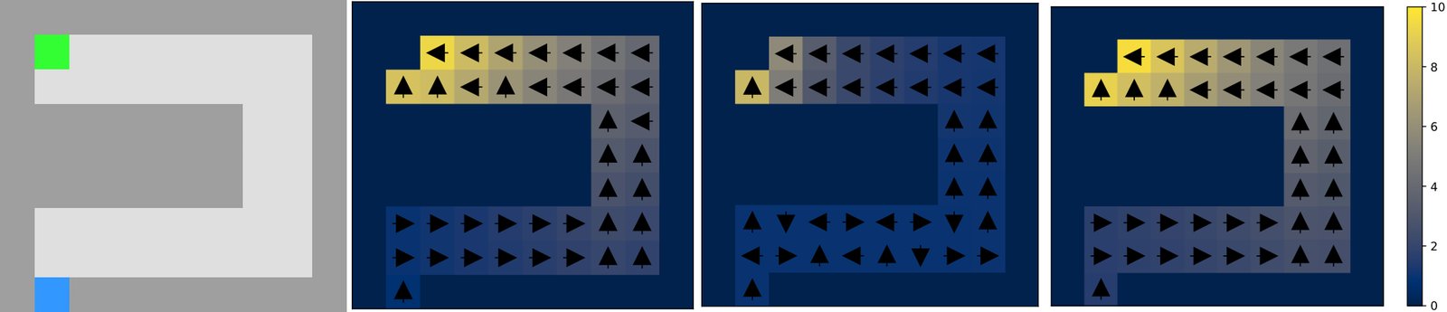
(a) toy maze MDP

(a) 玩具迷宫 MDP

图 2：玩具 umaze 环境上的算法评估。(a) 迷宫；(b) 真实最优 $V^{\star}$；(c) 单步策略评估；(d) IQL。

Figure 2 (c, d) illustrates the difference between single-step methods, in this case represented by Onepstep RL (Brandfonbrener et al. 2021; Wang et al. 2018) and IQL with $\tau=0.95$. Although states closer to the high reward state will still have higher values, these values decay much faster as we move further away than they would for the optimal value function, and the resulting policy is highly suboptimal. Since IQL (d) performs iterative dynamic programming, it correctly propagates the signal, and the values are no longer dominated by noise. The resulting value function closely matches the true optimal value function (b).

图 2 (c, d) 说明了单步方法——此处以 One-step RL（Brandfonbrener et al. 2021；Wang et al. 2018）为代表——与 $\tau=0.95$ 的 IQL 之间的差异。虽说离高奖励状态更近的状态仍有更高价值，但这些价值随距离衰减远快于最优价值函数，所得策略高度次优。IQL (d) 做迭代动态规划，能正确传播信号，价值不再被噪声主导；所得价值函数与真实最优价值函数 (b) 高度吻合。

5.2 Comparisons on Offline RL Benchmarks

5.2 离线 RL 基准上的比较

Dataset	BC	10%BC	DT	AWAC	Onestep RL	TD3+BC	CQL	IQL (Ours)
halfcheetah-medium-v2	42.6	42.5	42.6	43.5	48.4	48.3	44.0	47.4
hopper-medium-v2	52.9	56.9	67.6	57.0	59.6	59.3	58.5	66.3
walker2d-medium-v2	75.3	75.0	74.0	72.4	81.8	83.7	72.5	78.3
halfcheetah-medium-replay-v2	36.6	40.6	36.6	40.5	38.1	44.6	45.5	44.2
hopper-medium-replay-v2	18.1	75.9	82.7	37.2	97.5	60.9	95.0	94.7
walker2d-medium-replay-v2	26.0	62.5	66.6	27.0	49.5	81.8	77.2	73.9
halfcheetah-medium-expert-v2	55.2	92.9	86.8	42.8	93.4	90.7	91.6	86.7
hopper-medium-expert-v2	52.5	110.9	107.6	55.8	103.3	98.0	105.4	91.5
walker2d-medium-expert-v2	107.5	109.0	108.1	74.5	113.0	110.1	108.8	109.6
locomotion-v2 total	466.7	666.2	672.6	450.7	684.6	677.4	698.5	692.4
antmaze-umaze-v0	54.6	62.8	59.2	56.7	64.3	78.6	74.0	87.5
antmaze-umaze-diverse-v0	45.6	50.2	53.0	49.3	60.7	71.4	84.0	62.2
antmaze-medium-play-v0	0.0	5.4	0.0	0.0	0.3	10.6	61.2	71.2
antmaze-medium-diverse-v0	0.0	9.8	0.0	0.7	0.0	3.0	53.7	70.0
antmaze-large-play-v0	0.0	0.0	0.0	0.0	0.0	0.2	15.8	39.6
antmaze-large-diverse-v0	0.0	6.0	0.0	1.0	0.0	0.0	14.9	47.5
antmaze-v0 total	100.2	134.2	112.2	107.7	125.3	163.8	303.6	378.0
total	566.9	800.4	784.8	558.4	809.9	841.2	1002.1	1070.4
kitchen-v0 total	154.5	-	-	-	-	-	144.6	159.8
adroit-v0 total	104.5	-	-	-	-	-	93.6	118.1
total+kitchen+adroit	825.9	-	-	-	-	-	1240.3	1348.3
runtime	10m	10m	960m	20m	$\approx$ 20m∗	20m	80m	20m

Table 1: Averaged normalized scores on MuJoCo locomotion and Ant Maze tasks. Our method outperforms prior methods on the challenging Ant Maze tasks, which require dynamic programming, and is competitive with the best prior methods on the locomotion tasks.

Dataset	BC	10%BC	DT	AWAC	Onestep RL	TD3+BC	CQL	IQL (Ours)
halfcheetah-medium-v2	42.6	42.5	42.6	43.5	48.4	48.3	44.0	47.4
hopper-medium-v2	52.9	56.9	67.6	57.0	59.6	59.3	58.5	66.3
walker2d-medium-v2	75.3	75.0	74.0	72.4	81.8	83.7	72.5	78.3
halfcheetah-medium-replay-v2	36.6	40.6	36.6	40.5	38.1	44.6	45.5	44.2
hopper-medium-replay-v2	18.1	75.9	82.7	37.2	97.5	60.9	95.0	94.7
walker2d-medium-replay-v2	26.0	62.5	66.6	27.0	49.5	81.8	77.2	73.9
halfcheetah-medium-expert-v2	55.2	92.9	86.8	42.8	93.4	90.7	91.6	86.7
hopper-medium-expert-v2	52.5	110.9	107.6	55.8	103.3	98.0	105.4	91.5
walker2d-medium-expert-v2	107.5	109.0	108.1	74.5	113.0	110.1	108.8	109.6
locomotion-v2 total	466.7	666.2	672.6	450.7	684.6	677.4	698.5	692.4
antmaze-umaze-v0	54.6	62.8	59.2	56.7	64.3	78.6	74.0	87.5
antmaze-umaze-diverse-v0	45.6	50.2	53.0	49.3	60.7	71.4	84.0	62.2
antmaze-medium-play-v0	0.0	5.4	0.0	0.0	0.3	10.6	61.2	71.2
antmaze-medium-diverse-v0	0.0	9.8	0.0	0.7	0.0	3.0	53.7	70.0
antmaze-large-play-v0	0.0	0.0	0.0	0.0	0.0	0.2	15.8	39.6
antmaze-large-diverse-v0	0.0	6.0	0.0	1.0	0.0	0.0	14.9	47.5
antmaze-v0 total	100.2	134.2	112.2	107.7	125.3	163.8	303.6	378.0
total	566.9	800.4	784.8	558.4	809.9	841.2	1002.1	1070.4
kitchen-v0 total	154.5	-	-	-	-	-	144.6	159.8
adroit-v0 total	104.5	-	-	-	-	-	93.6	118.1
total+kitchen+adroit	825.9	-	-	-	-	-	1240.3	1348.3
runtime	10m	10m	960m	20m	$\approx$ 20m∗	20m	80m	20m

表 1：MuJoCo 运动与 Ant Maze 任务上的平均归一化分数。我们的方法在需要动态规划的困难 Ant Maze 任务上超过先前方法，在运动任务上与最优先前方法相当。

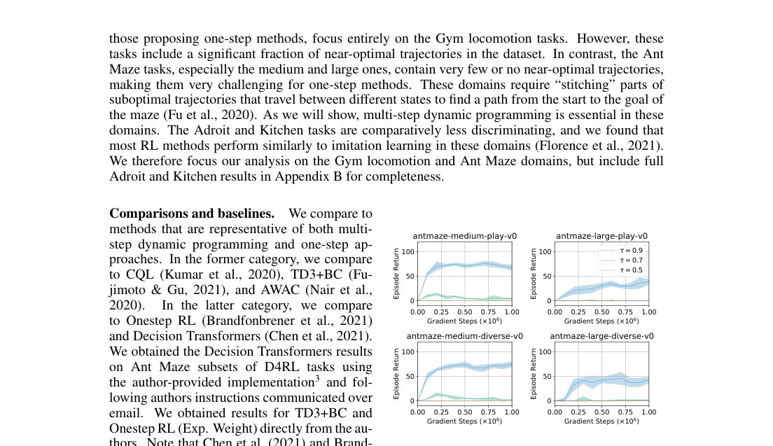
Figure 3: Estimating a larger expectile $\tau$ is crucial for antmaze tasks that require dynamical programming (’stitching’).

图 3：估计更大的 expectile $\tau$ 对需要动态规划（「缝合」）的 antmaze 任务至关重要。

Next, we evaluate our approach on the D4RL benchmark in comparison to prior methods (see Table 1). The MuJoCo tasks in D4RL consist of the Gym locomotion tasks, the Ant Maze tasks, and the Adroit and Kitchen robotic manipulation environments. Some prior works, particularly those proposing one-step methods, focus entirely on the Gym locomotion tasks. However, these tasks include a significant fraction of near-optimal trajectories in the dataset. In contrast, the Ant Maze tasks, especially the medium and large ones, contain very few or no near-optimal trajectories, making them very challenging for one-step methods. These domains require “stitching” parts of suboptimal trajectories that travel between different states to find a path from the start to the goal of the maze (Fu et al. 2020). As we will show, multi-step dynamic programming is essential in these domains. The Adroit and Kitchen tasks are comparatively less discriminating, and we found that most RL methods perform similarly to imitation learning in these domains (Florence et al. 2021). We therefore focus our analysis on the Gym locomotion and Ant Maze domains, but include full Adroit and Kitchen results in Appendix B for completeness.

接下来在 D4RL 基准上相对先前方法评估（见表 1）。D4RL 中的 MuJoCo 任务包括 Gym 运动任务、Ant Maze，以及 Adroit 与 Kitchen 机器人操作环境。部分先前工作——尤其提出单步方法者——几乎只关注 Gym 运动任务；这些任务的数据集里近优轨迹占比很高。相反，Ant Maze——尤其 medium 与 large——几乎没有或完全没有近优轨迹，对单步方法极具挑战。这些领域需要把连接不同状态的次优轨迹片段「缝合」起来，才能找到从起点到迷宫目标的路径（Fu et al. 2020）。如下所示，多步动态规划在这些领域必不可少。Adroit 与 Kitchen 区分度相对较低，我们发现多数 RL 方法在这些领域表现接近模仿学习（Florence et al. 2021）。因此分析聚焦 Gym 运动与 Ant Maze，完整 Adroit 与 Kitchen 结果见附录 B。

Comparisons and baselines.

We compare to methods that are representative of both multi-step dynamic programming and one-step approaches. In the former category, we compare to CQL (Kumar et al. 2020), TD3+BC (Fujimoto & Gu 2021), and AWAC (Nair et al. 2020). In the latter category, we compare to Onestep RL (Brandfonbrener et al. 2021) and Decision Transformers (Chen et al. 2021). We obtained the Decision Transformers results on Ant Maze subsets of D4RL tasks using the author-provided implementation[^3] and following authors instructions communicated over email. We obtained results for TD3+BC and Onestep RL (Exp. Weight) directly from the authors. Note that Chen et al. 2021 and Brandfonbrener et al. 2021 incorrectly report results for some prior methods, such as CQL, using the ‘‘-v0’’ environments. These generally produce lower scores than the ‘‘-v2’’ environments that these papers use for their own methods. We use the ‘‘-v2’’ environments for all methods to ensure a fair comparison, resulting in higher values for CQL. Because of this fix, our reported CQL scores are higher than all other prior methods. We obtained results for ‘‘-v2’’ datasets using an author-suggested implementation.[^4] On the Gym locomotion tasks (halfcheetah, hopper, walker2d), we find that IQL performs comparably to the best performing prior method, CQL. On the more challenging Ant Maze task, IQL outperforms CQL, and outperforms the one-step methods by a very large margin.

对比与基线。

我们与代表多步动态规划与单步两类方法的算法比较。前者包括 CQL（Kumar et al. 2020）、TD3+BC（Fujimoto & Gu 2021）与 AWAC（Nair et al. 2020）；后者包括 Onestep RL（Brandfonbrener et al. 2021）与 Decision Transformers（Chen et al. 2021）。Ant Maze 子集上的 Decision Transformers 结果使用作者提供的实现[^3]，并按作者邮件说明操作。TD3+BC 与 Onestep RL（Exp. Weight）结果直接来自作者。注意 Chen et al. 2021 与 Brandfonbrener et al. 2021 对部分先前方法（如 CQL）误报了「-v0」环境结果；这些通常低于它们自己方法所用的「-v2」。为保证公平，我们对所有方法使用「-v2」，从而使 CQL 分数更高。经此修正，我们报告的 CQL 分数高于所有其他先前方法。「-v2」结果使用作者建议的实现。[^4] 在 Gym 运动任务（halfcheetah、hopper、walker2d）上，IQL 与表现最好的先前方法 CQL 相当；在更难的 Ant Maze 上，IQL 超过 CQL，并以很大优势超过单步方法。

Runtime.

Our approach is also computationally faster than the baselines (see Table 1). For the baselines, we measure runtime for our reimplementations of the methods in JAX (Bradbury et al. 2018) built on top of JAXRL (Kostrikov 2021), which are typically faster than the original implementations. For example, the original implementation of CQL takes more than 4 hours to perform 1M updates, while ours takes only 80 minutes. Even so, IQL still requires about 4x less time than our reimplementation of CQL on average, and is comparable to the fastest prior one-step methods. We did not reimplement Decision Transformers due to their complexity and report runtime of the original implementation.

运行时间。

我们的方法也比基线计算更快（见表 1）。对基线，我们测量的是基于 JAX（Bradbury et al. 2018）、构建在 JAXRL（Kostrikov 2021）上的重实现运行时间，通常快于原始实现。例如 CQL 原始实现做 100 万次更新要超过 4 小时，我们的重实现只需 80 分钟。即便如此，IQL 平均仍比我们的 CQL 重实现大约快 4 倍，并与最快的先前单步方法相当。因 Decision Transformers 较复杂，我们未重实现，报告的是原始实现运行时间。

Effect of $\tau$ hyperparameter.

We also demonstrate that it is crucial to compute a larger expectile on tasks that require “stitching” (see Figure 3). With larger values of $\tau$, our method approximates $Q$-learning better, leading to better performance on the Ant Maze tasks.

$\tau$ 超参数的影响。

我们还表明：在需要「缝合」的任务上，计算更大的 expectile 至关重要（见图 3）。$\tau$ 越大，方法越接近近似 $Q$-learning，Ant Maze 上的表现也越好。

5.3 Online Fine-tuning after Offline RL

5.3 离线 RL 之后的在线微调

Dataset	AWAC	CQL	IQL (Ours)
antmaze-umaze-v0	56.7   $\rightarrow$ 59.0	70.1   $\rightarrow$ 99.4	86.7   $\rightarrow$ 96.0
antmaze-umaze-diverse-v0	49.3   $\rightarrow$ 49.0	31.1   $\rightarrow$ 99.4	75.0   $\rightarrow$ 84.0
antmaze-medium-play-v0	0.0     $\rightarrow$ 0.0	23.0   $\rightarrow$ 0.0	72.0   $\rightarrow$ 95.0
antmaze-medium-diverse-v0	0.7     $\rightarrow$ 0.3	23.0   $\rightarrow$ 32.3	68.3   $\rightarrow$ 92.0
antmaze-large-play-v0	0.0     $\rightarrow$ 0.0	1.0     $\rightarrow$ 0.0	25.5   $\rightarrow$ 46.0
antmaze-large-diverse-v0	1.0     $\rightarrow$ 0.0	1.0     $\rightarrow$ 0.0	42.6   $\rightarrow$ 60.7
antmaze-v0 total	107.7 $\rightarrow$ 108.3	151.5 $\rightarrow$ 231.1	370.1 $\rightarrow$ 473.7
pen-binary-v0	44.6   $\rightarrow$ 70.3	31.2   $\rightarrow$ 9.9	37.4   $\rightarrow$ 60.7
door-binary-v0	1.3     $\rightarrow$ 30.1	0.2     $\rightarrow$ 0.0	0.7     $\rightarrow$ 32.3
relocate-binary-v0	0.8     $\rightarrow$ 2.7	0.1     $\rightarrow$ 0.0	0.0     $\rightarrow$ 31.0
hand-v0 total	46.7   $\rightarrow$ 103.1	31.5   $\rightarrow$ 9.9	38.1   $\rightarrow$ 124.0
total	154.4 $\rightarrow$ 211.4	182.8 $\rightarrow$ 241.0	408.2 $\rightarrow$ 597.7

Table 2: Online finetuning results showing the initial performance after offline RL, and performance after 1M steps of online RL. In all tasks, IQL is able to finetune to a significantly higher performance than the offline initialization, with final performance that is comparable to or better than the best of either AWAC or CQL on all tasks except pen-binary-v0.

Dataset	AWAC	CQL	IQL (Ours)
antmaze-umaze-v0	56.7   $\rightarrow$ 59.0	70.1   $\rightarrow$ 99.4	86.7   $\rightarrow$ 96.0
antmaze-umaze-diverse-v0	49.3   $\rightarrow$ 49.0	31.1   $\rightarrow$ 99.4	75.0   $\rightarrow$ 84.0
antmaze-medium-play-v0	0.0     $\rightarrow$ 0.0	23.0   $\rightarrow$ 0.0	72.0   $\rightarrow$ 95.0
antmaze-medium-diverse-v0	0.7     $\rightarrow$ 0.3	23.0   $\rightarrow$ 32.3	68.3   $\rightarrow$ 92.0
antmaze-large-play-v0	0.0     $\rightarrow$ 0.0	1.0     $\rightarrow$ 0.0	25.5   $\rightarrow$ 46.0
antmaze-large-diverse-v0	1.0     $\rightarrow$ 0.0	1.0     $\rightarrow$ 0.0	42.6   $\rightarrow$ 60.7
antmaze-v0 total	107.7 $\rightarrow$ 108.3	151.5 $\rightarrow$ 231.1	370.1 $\rightarrow$ 473.7
pen-binary-v0	44.6   $\rightarrow$ 70.3	31.2   $\rightarrow$ 9.9	37.4   $\rightarrow$ 60.7
door-binary-v0	1.3     $\rightarrow$ 30.1	0.2     $\rightarrow$ 0.0	0.7     $\rightarrow$ 32.3
relocate-binary-v0	0.8     $\rightarrow$ 2.7	0.1     $\rightarrow$ 0.0	0.0     $\rightarrow$ 31.0
hand-v0 total	46.7   $\rightarrow$ 103.1	31.5   $\rightarrow$ 9.9	38.1   $\rightarrow$ 124.0
total	154.4 $\rightarrow$ 211.4	182.8 $\rightarrow$ 241.0	408.2 $\rightarrow$ 597.7

表 2：在线微调结果：离线 RL 后的初始表现，以及再做 100 万步在线 RL 后的表现。在所有任务上，IQL 都能微调到显著高于离线初始化的水平；最终表现在除 pen-binary-v0 外的全部任务上与 AWAC 或 CQL 中较好者相当或更好。

The policies obtained by offline RL can often be improved with a small amount of online interaction. IQL is well-suited for online fine-tuning for two reasons. First, IQL has strong offline performance, as shown in the previous section, which provides a good initialization. Second, IQL implements a weighted behavioral cloning policy extraction step, which has previously been shown to allow for better online policy improvement compared to other types of offline constraints (Nair et al. 2020). To evaluate the finetuning capability of various RL algorithms, we first run offline RL on each dataset, then run 1M steps of online RL, and then report the final performance. We compare to AWAC (Nair et al. 2020), which has been proposed specifically for online finetuning, and CQL (Kumar et al. 2020), which showed the best performance among prior methods in our experiments in the previous section. Exact experimental details are provided in Appendix C. We use the challenging Ant Maze D4RL domains (Fu et al. 2020), as well as the high-dimensional dexterous manipulation environments from Rajeswaran et al. 2018, which Nair et al. 2020 propose to use to study online adaptation with AWAC. Results are shown in Table 2. On the Ant Maze domains, IQL significantly outperforms both prior methods after online finetuning. CQL attains the second best score, while AWAC performs comparatively worse due to much weaker offline initialization. On the dexterous hand tasks, IQL performs significantly better than AWAC on relocate-binary-v0, comparably on door-binary-v0, and slightly worse on pen-binary-v0, with the best overall score.

离线 RL 得到的策略常可再用少量在线交互改进。IQL 适于在线微调有两点原因。第一，如前一节所示，IQL 离线表现强，提供良好初始化；第二，IQL 用加权行为克隆做策略抽取，先前已表明这类方式相对其他离线约束更利于在线策略改进（Nair et al. 2020）。为评估各 RL 算法的微调能力，我们先在每个数据集上跑离线 RL，再跑 100 万步在线 RL，报告最终表现。对比对象为专为在线微调提出的 AWAC（Nair et al. 2020），以及上一节实验中先前方法里表现最好的 CQL（Kumar et al. 2020）。精确实验细节见附录 C。我们使用困难的 Ant Maze D4RL 领域（Fu et al. 2020），以及 Rajeswaran et al. 2018 的高维灵巧操作环境（Nair et al. 2020 建议用其研究 AWAC 的在线适应）。结果见表 2。在 Ant Maze 上，在线微调后 IQL 显著超过两种先前方法；CQL 次之，AWAC 因离线初始化弱得多而相对较差。在灵巧手任务上，IQL 在 relocate-binary-v0 上显著好于 AWAC，在 door-binary-v0 上相当，在 pen-binary-v0 上略差，总体分数最好。

6 Conclusion

6 结论

We presented implicit Q-Learning (IQL), a general algorithm for offline RL that completely avoids any queries to values of out-of-sample actions during training while still enabling multi-step dynamic programming. To our knowledge, this is the first method that combines both of these features. This has a number of important benefits. First, our algorithm is computationally efficient: we can perform 1M updates on one GTX1080 GPU in less than 20 minutes. Second, it is simple to implement, requiring only minor modifications over a standard SARSA-like TD algorithm, and performing policy extraction with a simple weighted behavioral cloning procedure resembling supervised learning. Finally, despite the simplicity and efficiency of this method, we show that it attains excellent performance across all of the tasks in the D4RL benchmark, matching the best prior methods on the MuJoCo locomotion tasks, and exceeding the state-of-the-art performance on the challenging ant maze environments, where multi-step dynamic programming is essential for good performance.

我们提出隐式 Q 学习（IQL）：一种通用离线 RL 算法，训练时完全避免查询样本外动作的价值，却仍能做多步动态规划。据我们所知，这是首个同时具备这两点的方法。好处包括：第一，计算高效——在一块 GTX1080 GPU 上做 100 万次更新不到 20 分钟；第二，实现简单——只需对标准类 SARSA TD 算法做小改，并用类似监督学习的加权行为克隆抽取策略；第三，尽管简洁高效，它在 D4RL 全部任务上表现优异：MuJoCo 运动任务上匹配最优先前方法，在必须靠多步动态规划才能表现好的困难 ant maze 环境上超过当时最优。

References

参考文献

Bradbury et al. (2018) James Bradbury, Roy Frostig, Peter Hawkins, Matthew James Johnson, Chris Leary, Dougal Maclaurin, George Necula, Adam Paszke, Jake VanderPlas, Skye Wanderman-Milne, and Qiao Zhang. JAX: composable transformations of Python+NumPy programs, 2018. URL http://github.com/google/jax .

Brandfonbrener et al. (2021) David Brandfonbrener, William F Whitney, Rajesh Ranganath, and Joan Bruna. Offline rl without off-policy evaluation. arXiv preprint arXiv:2106.08909 , 2021.

Chen et al. (2021) Lili Chen, Kevin Lu, Aravind Rajeswaran, Kimin Lee, Aditya Grover, Michael Laskin, Pieter Abbeel, Aravind Srinivas, and Igor Mordatch. Decision transformer: Reinforcement learning via sequence modeling. arXiv preprint arXiv:2106.01345 , 2021.

Dabney et al. (2018a) Will Dabney, Georg Ostrovski, David Silver, and Rémi Munos. Implicit quantile networks for distributional reinforcement learning. In International conference on machine learning , pp. 1096–1105. PMLR, 2018a.

Dabney et al. (2018b) Will Dabney, Mark Rowland, Marc G Bellemare, and Rémi Munos. Distributional reinforcement learning with quantile regression. In Thirty-Second AAAI Conference on Artificial Intelligence , 2018b.

Florence et al. (2021) Pete Florence, Corey Lynch, Andy Zeng, Oscar Ramirez, Ayzaan Wahid, Laura Downs, Adrian Wong, Johnny Lee, Igor Mordatch, and Jonathan Tompson. Implicit behavioral cloning. arXiv preprint arXiv:2109.00137 , 2021.

Fu et al. (2020) Justin Fu, Aviral Kumar, Ofir Nachum, George Tucker, and Sergey Levine. D4rl: Datasets for deep data-driven reinforcement learning. arXiv preprint arXiv:2004.07219 , 2020.

Fujimoto & Gu (2021) Scott Fujimoto and Shixiang Shane Gu. A minimalist approach to offline reinforcement learning. arXiv preprint arXiv:2106.06860 , 2021.

Fujimoto et al. (2018) Scott Fujimoto, Herke Hoof, and David Meger. Addressing function approximation error in actor-critic methods. In International Conference on Machine Learning , pp. 1587–1596. PMLR, 2018.

Fujimoto et al. (2019) Scott Fujimoto, David Meger, and Doina Precup. Off-policy deep reinforcement learning without exploration. In International Conference on Machine Learning , pp. 2052–2062. PMLR, 2019.

Heek et al. (2020) Jonathan Heek, Anselm Levskaya, Avital Oliver, Marvin Ritter, Bertrand Rondepierre, Andreas Steiner, and Marc van Zee. Flax: A neural network library and ecosystem for JAX, 2020. URL http://github.com/google/flax .

Kingma & Ba (2014) Diederik P Kingma and Jimmy Ba. Adam: A method for stochastic optimization. arXiv preprint arXiv:1412.6980 , 2014.

Koenker & Hallock (2001) Roger Koenker and Kevin F Hallock. Quantile regression. Journal of economic perspectives , 15(4):143–156, 2001.

Kostrikov (2021) Ilya Kostrikov. JAXRL: Implementations of Reinforcement Learning algorithms in JAX., 10 2021. URL https://github.com/ikostrikov/jaxrl .

Kostrikov et al. (2021) Ilya Kostrikov, Rob Fergus, Jonathan Tompson, and Ofir Nachum. Offline reinforcement learning with fisher divergence critic regularization. In International Conference on Machine Learning , pp. 5774–5783. PMLR, 2021.

Kumar et al. (2019) Aviral Kumar, Justin Fu, George Tucker, and Sergey Levine. Stabilizing off-policy q-learning via bootstrapping error reduction. arXiv preprint arXiv:1906.00949 , 2019.

Kumar et al. (2020) Aviral Kumar, Aurick Zhou, George Tucker, and Sergey Levine. Conservative q-learning for offline reinforcement learning. arXiv preprint arXiv:2006.04779 , 2020.

Kuznetsov et al. (2020) Arsenii Kuznetsov, Pavel Shvechikov, Alexander Grishin, and Dmitry Vetrov. Controlling overestimation bias with truncated mixture of continuous distributional quantile critics. In International Conference on Machine Learning , pp. 5556–5566. PMLR, 2020.

Lange et al. (2012) Sascha Lange, Thomas Gabel, and Martin Riedmiller. Batch reinforcement learning. In Reinforcement learning , pp. 45–73. Springer, 2012.

Nair et al. (2020) Ashvin Nair, Murtaza Dalal, Abhishek Gupta, and Sergey Levine. Awac: Accelerating online reinforcement learning with offline datasets. 2020.

Peng et al. (2019) Xue Bin Peng, Aviral Kumar, Grace Zhang, and Sergey Levine. Advantage-weighted regression: Simple and scalable off-policy reinforcement learning. arXiv preprint arXiv:1910.00177 , 2019.

Peters & Schaal (2007) Jan Peters and Stefan Schaal. Reinforcement learning by reward-weighted regression for operational space control. In Proceedings of the 24th international conference on Machine learning , pp. 745–750, 2007.

Rajeswaran et al. (2018) Aravind Rajeswaran, Vikash Kumar, Abhishek Gupta, John Schulman, Emanuel Todorov, and Sergey Levine. Learning Complex Dexterous Manipulation with Deep Reinforcement Learning and Demonstrations. In Robotics: Science and Systems , 2018. URL https://arxiv.org/pdf/1709.10087.pdf .

Srivastava et al. (2014) Nitish Srivastava, Geoffrey Hinton, Alex Krizhevsky, Ilya Sutskever, and Ruslan Salakhutdinov. Dropout: a simple way to prevent neural networks from overfitting. The journal of machine learning research , 15(1):1929–1958, 2014.

Sutton & Barto (2018) Richard S Sutton and Andrew G Barto. Reinforcement learning: An introduction . MIT press, 2018.

Wang et al. (2018) Qing Wang, Jiechao Xiong, Lei Han, Peng Sun, Han Liu, and Tong Zhang. Exponentially weighted imitation learning for batched historical data. In NeurIPS , pp. 6291–6300, 2018.

Wang et al. (2020) Ziyu Wang, Alexander Novikov, Konrad Zolna, Jost Tobias Springenberg, Scott Reed, Bobak Shahriari, Noah Siegel, Josh Merel, Caglar Gulcehre, Nicolas Heess, et al. Critic regularized regression. arXiv preprint arXiv:2006.15134 , 2020.

Wu et al. (2019) Yifan Wu, George Tucker, and Ofir Nachum. Behavior regularized offline reinforcement learning. arXiv preprint arXiv:1911.11361 , 2019.

Appendix A Proofs

附录 A 证明

A.1 Proof of Lemma 2

A.1 引理 2 的证明

Proof.

We can rewrite $V_{\tau_{1}}(s)$ as

证明。

$$\displaystyle V_{\tau_{1}}(s) \\ \displaystyle=\mathbb{E}^{\tau_{1}}_{a\sim\mu(\cdot|s)}[r(s,a)+\gamma\mathbb{E}_{s^{\prime}\sim p(\cdot|s,a)}[V_{\tau_{1}}(s^{\prime})]] \\ \displaystyle\leq\mathbb{E}^{\tau_{2}}_{a\sim\mu(\cdot|s)}[r(s,a)+\gamma\mathbb{E}_{s^{\prime}\sim p(\cdot|s,a)}[V_{\tau_{1}}(s^{\prime})]] \\ \displaystyle=\mathbb{E}^{\tau_{2}}_{a\sim\mu(\cdot|s)}[r(s,a)+\gamma\mathbb{E}_{s^{\prime}\sim p(\cdot|s,a)}\mathbb{E}^{\tau_{1}}_{a^{\prime}\sim\mu(\cdot|s^{\prime})}[r(s^{\prime},a^{\prime})+\gamma\mathbb{E}_{s^{\prime\prime}\sim p(\cdot|s^{\prime},a^{\prime})}[V_{\tau_{1}}(s^{\prime\prime})]] \\ \displaystyle\leq\mathbb{E}^{\tau_{2}}_{a\sim\mu(\cdot|s)}[r(s,a)+\gamma\mathbb{E}_{s^{\prime}\sim p(\cdot|s,a)}\mathbb{E}^{\tau_{2}}_{a^{\prime}\sim\mu(\cdot|s^{\prime})}[r(s^{\prime},a^{\prime})+\gamma\mathbb{E}_{s^{\prime\prime}\sim p(\cdot|s^{\prime},a^{\prime})}[V_{\tau_{1}}(s^{\prime\prime})]] \\ \displaystyle=\mathbb{E}^{\tau_{2}}_{a\sim\mu(\cdot|s)}[r(s,a)+\gamma\mathbb{E}_{s^{\prime}\sim p(\cdot|s,a)}\mathbb{E}^{\tau_{2}}_{a^{\prime}\sim\mu(\cdot|s^{\prime})}[r(s^{\prime},a^{\prime})+\gamma\mathbb{E}_{s^{\prime\prime}\sim p(\cdot|s^{\prime},a^{\prime})}\mathbb{E}^{\tau_{1}}_{a^{\prime\prime}\sim\mu(\cdot|s^{\prime\prime})}[r(s^{\prime\prime},a^{\prime\prime})+\ldots]] \\ \displaystyle\leq V_{\tau_{2}}(s)$$

$$\displaystyle V_{\tau_{1}}(s) \\ \displaystyle=\mathbb{E}^{\tau_{1}}_{a\sim\mu(\cdot|s)}[r(s,a)+\gamma\mathbb{E}_{s^{\prime}\sim p(\cdot|s,a)}[V_{\tau_{1}}(s^{\prime})]] \\ \displaystyle\leq\mathbb{E}^{\tau_{2}}_{a\sim\mu(\cdot|s)}[r(s,a)+\gamma\mathbb{E}_{s^{\prime}\sim p(\cdot|s,a)}[V_{\tau_{1}}(s^{\prime})]] \\ \displaystyle=\mathbb{E}^{\tau_{2}}_{a\sim\mu(\cdot|s)}[r(s,a)+\gamma\mathbb{E}_{s^{\prime}\sim p(\cdot|s,a)}\mathbb{E}^{\tau_{1}}_{a^{\prime}\sim\mu(\cdot|s^{\prime})}[r(s^{\prime},a^{\prime})+\gamma\mathbb{E}_{s^{\prime\prime}\sim p(\cdot|s^{\prime},a^{\prime})}[V_{\tau_{1}}(s^{\prime\prime})]]] \\ \displaystyle\leq\mathbb{E}^{\tau_{2}}_{a\sim\mu(\cdot|s)}[r(s,a)+\gamma\mathbb{E}_{s^{\prime}\sim p(\cdot|s,a)}\mathbb{E}^{\tau_{2}}_{a^{\prime}\sim\mu(\cdot|s^{\prime})}[r(s^{\prime},a^{\prime})+\gamma\mathbb{E}_{s^{\prime\prime}\sim p(\cdot|s^{\prime},a^{\prime})}[V_{\tau_{1}}(s^{\prime\prime})]]] \\ \displaystyle=\mathbb{E}^{\tau_{2}}_{a\sim\mu(\cdot|s)}[r(s,a)+\gamma\mathbb{E}_{s^{\prime}\sim p(\cdot|s,a)}\mathbb{E}^{\tau_{2}}_{a^{\prime}\sim\mu(\cdot|s^{\prime})}[r(s^{\prime},a^{\prime})+\gamma\mathbb{E}_{s^{\prime\prime}\sim p(\cdot|s^{\prime},a^{\prime})}\mathbb{E}^{\tau_{1}}_{a^{\prime\prime}\sim\mu(\cdot|s^{\prime\prime})}[r(s^{\prime\prime},a^{\prime\prime})+\ldots]]] \\ \displaystyle\leq V_{\tau_{2}}(s)$$

∎

Appendix B Experimental details

附录 B 实验细节

Experimental details.

For the MuJoCo locomotion tasks, we average mean returns overs 10 evaluation trajectories and 10 random seeds. For the Ant Maze tasks, we average over 100 evaluation trajectories. We standardize MuJoCo locomotion task rewards by dividing by the difference of returns of the best and worst trajectories in each dataset. Following the suggestions of the authors of the dataset, we subtract $1$ from rewards for the Ant Maze datasets. We use $\tau=0.9$ and $\beta=10.0$ for Ant Maze tasks and $\tau=0.7$ and $\beta=3.0$ for MuJoCo locomotion tasks. We use Adam optimizer (Kingma & Ba 2014) with a learning rate $3\cdot 10^{-4}$ and 2 layer MLP with ReLU activations and 256 hidden units for all networks. We use cosine schedule for the actor learning rate. We parameterize the policy as a Gaussian distribution with a state-independent standard deviation. We update the target network with soft updates with parameter $\alpha=0.005$. And following Brandfonbrener et al. 2021 we clip exponentiated advantages to $(-\infty,100]$. We implemented our method in the JAX (Bradbury et al. 2018) framework using the Flax (Heek et al. 2020) neural networks library.

实验细节。

MuJoCo 运动任务上，我们对 10 条评估轨迹与 10 个随机种子平均回报均值；Ant Maze 任务上对 100 条评估轨迹取平均。MuJoCo 运动任务奖励按各数据集中最好与最差轨迹回报之差做标准化。按数据集作者建议，Ant Maze 奖励减 $1$。Ant Maze 取 $\tau=0.9$、$\beta=10.0$；MuJoCo 运动取 $\tau=0.7$、$\beta=3.0$。优化器用 Adam（Kingma & Ba 2014），学习率 $3\cdot 10^{-4}$；所有网络为带 ReLU、隐层 256 的两层 MLP。actor 学习率用余弦调度。策略参数化为状态无关标准差的高斯。目标网络软更新参数 $\alpha=0.005$。按 Brandfonbrener et al. 2021，将指数化优势裁剪到 $(-\infty,100]$。方法在 JAX（Bradbury et al. 2018）上实现，神经网络库为 Flax（Heek et al. 2020）。

Results on Franca Kitchen and Adoit tasks.

For Franca Kitchen and Adroit tasks we use $\tau=0.7$ and the inverse temperature $\beta=0.5$. Due to the size of the dataset, we also apply Dropout (Srivastava et al. 2014) with dropout rate of $0.1$ to regularize the policy network. See complete results in Table 3.

Franca Kitchen 与 Adroit 任务结果。

Franca Kitchen 与 Adroit 任务取 $\tau=0.7$、逆温度 $\beta=0.5$。因数据集规模，还对策略网络施加 Dropout（Srivastava et al. 2014），dropout 率 $0.1$。完整结果见表 3。

dataset	BC	BRAC-p	BEAR	Onestep RL	CQL	Ours
kitchen-complete-v0	65.0	0.0	0.0	-	43.8	62.5
kitchen-partial-v0	38.0	0.0	0.0	-	49.8	46.3
kitchen-mixed-v0	51.5	0.0	0.0	-	51.0	51.0
kitchen-v0 total	154.5	0.0	0.0	-	144.6	159.8
pen-human-v0	63.9	8.1	-1.0	-	37.5	71.5
hammer-human-v0	1.2	0.3	0.3	-	4.4	1.4
door-human-v0	2	-0.3	-0.3	-	9.9	4.3
relocate-human-v0	0.1	-0.3	-0.3	-	0.2	0.1
pen-cloned-v0	37	1.6	26.5	60.0	39.2	37.3
hammer-cloned-v0	0.6	0.3	0.3	2.1	2.1	2.1
door-cloned-v0	0.0	-0.1	-0.1	0.4	0.4	1.6
relocate-cloned-v0	-0.3	-0.3	-0.3	-0.1	-0.1	-0.2
adroit-v0 total	104.5	9.3	25.1	-	93.6	118.1
total	259	9.3	25.1	-	238.2	277.9

Table 3: Evaluation on Franca Kitchen and Adroit tasks from D4RL

dataset	BC	BRAC-p	BEAR	Onestep RL	CQL	Ours
kitchen-complete-v0	65.0	0.0	0.0	-	43.8	62.5
kitchen-partial-v0	38.0	0.0	0.0	-	49.8	46.3
kitchen-mixed-v0	51.5	0.0	0.0	-	51.0	51.0
kitchen-v0 total	154.5	0.0	0.0	-	144.6	159.8
pen-human-v0	63.9	8.1	-1.0	-	37.5	71.5
hammer-human-v0	1.2	0.3	0.3	-	4.4	1.4
door-human-v0	2	-0.3	-0.3	-	9.9	4.3
relocate-human-v0	0.1	-0.3	-0.3	-	0.2	0.1
pen-cloned-v0	37	1.6	26.5	60.0	39.2	37.3
hammer-cloned-v0	0.6	0.3	0.3	2.1	2.1	2.1
door-cloned-v0	0.0	-0.1	-0.1	0.4	0.4	1.6
relocate-cloned-v0	-0.3	-0.3	-0.3	-0.1	-0.1	-0.2
adroit-v0 total	104.5	9.3	25.1	-	93.6	118.1
total	259	9.3	25.1	-	238.2	277.9

表 3：D4RL 上 Franca Kitchen 与 Adroit 任务的评估

Appendix C Finetuning experimental details

附录 C 微调实验细节

For finetuning experiments, we first run offline RL for 1M gradient steps. Then we continue training while collecting data actively in the environment and adding that data to the replay buffer, running 1 gradient update / environment step. All other training details are kept the same between the offline RL phase and the online RL phase. For dextrous manipulation environments (Rajeswaran et al. 2018), we use $\tau=0.8$ and $\beta=3.0$, 25000 offline training steps, and add Gaussian noise with standard deviation $\sigma=0.03$ to the policy for exploration.

微调实验中，先离线 RL 训练 100 万梯度步；随后在继续训练的同时主动在环境中采集数据并加入回放缓冲，按 1 次梯度更新 / 环境步运行。离线与在线阶段其余训练细节保持一致。灵巧操作环境（Rajeswaran et al. 2018）取 $\tau=0.8$、$\beta=3.0$，离线训练 25000 步，并为探索给策略加标准差 $\sigma=0.03$ 的高斯噪声。

For baselines we compare to the original implementations of AWAC (Nair et al. 2020) and CQL (Kumar et al. 2020). For AWAC we used https://github.com/rail-berkeley/rlkit/tree/master/rlkit. We found AWAC to overfit heavily with too many offline gradient steps, and instead used 25000 offline gradient steps as in the original paper. For the dextrous manipulation results, we report average return normalized from 0 to 100 for consistency, instead of success rate at the final timestep, as reported in (Nair et al. 2020). For CQL, we used https://github.com/aviralkumar2907/CQL. Our reproduced results offline are worse than the reported results, particularly on medium and large antmaze environments. We were not able to improve these results after checking for discrepancies with the CQL paper authors and running CQL with an alternative implementation (https://github.com/tensorflow/agents). Thus, although for offline experiments (Table 2) we report results from the original paper, for finetuning experiments we did not have this option and report our own results running CQL in Table 2.

基线对比使用 AWAC（Nair et al. 2020）与 CQL（Kumar et al. 2020）的原始实现。AWAC 使用 https://github.com/rail-berkeley/rlkit/tree/master/rlkit。我们发现 AWAC 在离线梯度步过多时严重过拟合，因而按原论文使用 25000 离线梯度步。灵巧操作结果报告 0 到 100 的归一化平均回报以保持一致，而非（Nair et al. 2020）中的最终时间步成功率。CQL 使用 https://github.com/aviralkumar2907/CQL。我们复现的离线结果弱于论文报告，尤其在 medium 与 large antmaze 上。与 CQL 论文作者核对差异并用另一实现（https://github.com/tensorflow/agents）跑过后仍未能改善。因此，离线实验（表 2）我们报告原论文结果；微调实验无法如此，表 2 中报告的是我们自行运行 CQL 的结果。

Appendix D Connections to prior work

附录 D 与先前工作的联系

In this section, we discuss how our approach is related to prior work on offline reinforcement learning. In particular, we discuss connections to BCQ Fujimoto et al. 2019.

本节讨论我们的方法与先前离线强化学习工作的关系，尤其与 BCQ（Fujimoto et al. 2019）的联系。

Our batch constrained optimization objective is similar to BCQ (Fujimoto et al. 2019). In particular, the authors of BCQ build on the Q-learning framework and define the policy as

我们的批次约束优化目标与 BCQ（Fujimoto et al. 2019）相似。具体而言，BCQ 作者建立在 Q-learning 框架上，将策略定义为

$$\pi(s)=\argmax_{\begin{subarray}{c}a\
s.t.(s,a)\in\mathcal{D}\end{subarray}}Q(s,a). \tag{8}$$

$$\pi(s)=\argmax_{\begin{subarray}{c}a\\ s.t.(s,a)\in\mathcal{D}\end{subarray}}Q(s,a). \tag{8}$$

Note that in contrast to the standard Q-learning, maximization in Equation 8 is performed only over the state-action pairs that appear in the dataset. In Fujimoto et al. 2019, these constraints are implemented via fitting a generative model $\mu(\cdot|s)$ on the dataset, sampling several candidate actions from this generative model, and taking an argmax over these actions:

注意与标准 Q-learning 不同，公式 8 的最大化只在数据集中出现的状态–动作对上进行。Fujimoto et al. 2019 通过在数据集上拟合生成模型 $\mu(\cdot|s)$、从中采样若干候选动作、再对这些动作取 argmax 来实现约束：

$$\pi(s)=\argmax_{\{a_{i}|a_{i}\sim\mu(\cdot|s),i=1\ldots N\}}Q(s,a_{i}).$$

However, this generative model can still produce out-of-dataset actions that will lead to querying undefined Q-values. Thus, our work introduces an alternative way to optimize this objective without requiring an additional density model. Our approach avoids this issue by enforcing the hard constraints via estimating expectiles. Also, it is worth mentioning that a number of sampled actions $N$ in BCQ has similar properties to choosing a particular expectile $\tau$ in our approach.

但该生成模型仍可能产生数据集外动作，从而查询到未定义的 $Q$ 值。因此本文引入另一种优化该目标的方式，无需额外密度模型：通过估计 expectile 施加硬约束来避免该问题。另需指出，BCQ 中采样动作数 $N$ 与我们方法中选取特定 expectile $\tau$ 具有相似性质。

Note that our algorithm for optimal value approximation does not require an explicit policy, in contrast to other algorithms for offline reinforcement learning for continuous action spaces (Fujimoto et al. 2019; Fujimoto & Gu 2021; Wu et al. 2019; Kostrikov et al. 2021; Kumar et al. 2019; Kumar et al. 2020). Thus, we do not need to alternate between actor and critic updates, though with continuous actions, we must still extract an actor at the end once the critic converges.

注意我们的最优价值近似算法不需要显式策略，这与连续动作空间上的其他离线强化学习算法不同（Fujimoto et al. 2019；Fujimoto & Gu 2021；Wu et al. 2019；Kostrikov et al. 2021；Kumar et al. 2019；Kumar et al. 2020）。因此不必在 actor 与 critic 更新之间交替；不过在连续动作下，critic 收敛后仍须抽取 actor。