Understanding Black-box Predictions via Influence Functions
Understanding Black-box Predictions via Influence Functions
Understanding Black-box Predictions via Influence Functions:用影响函数理解黑盒预测
Abstract
摘要
How can we explain the predictions of a black-box model? In this paper, we use influence functions — a classic technique from robust statistics — to trace a model’s prediction through the learning algorithm and back to its training data, thereby identifying training points most responsible for a given prediction. To scale up influence functions to modern machine learning settings, we develop a simple, efficient implementation that requires only oracle access to gradients and Hessian-vector products. We show that even on non-convex and non-differentiable models where the theory breaks down, approximations to influence functions can still provide valuable information. On linear models and convolutional neural networks, we demonstrate that influence functions are useful for multiple purposes: understanding model behavior, debugging models, detecting dataset errors, and even creating visually-indistinguishable training-set attacks.
怎样解释黑盒模型的预测?本文将稳健统计里的经典工具——影响函数——用来沿学习算法把一次预测追回到训练数据,从而找出对这次预测最该负责的训练点。为了把影响函数做到现代机器学习的规模,我们给出一种只需梯度与 Hessian-向量积预言机的简单、高效实现。我们还表明,即便在理论假定不再成立的非凸、不可微模型上,影响函数的近似仍然能提供有用信息。在线性模型和卷积神经网络上,影响函数可以同时服务于多种用途:理解模型行为、调试模型、发现数据错误,甚至构造肉眼几乎分不出的训练集攻击。
1. Introduction
1. 引言
A key question often asked of machine learning systems is “Why did the system make this prediction?” We want models that are not just high-performing but also explainable. By understanding why a model does what it does, we can hope to improve the model (Amershi et al., 2015), discover new science (Shrikumar et al., 2016), and provide end-users with explanations of actions that impact them (Goodman & Flaxman, 2016).
机器学习系统常被问到的一个关键问题是:“系统为什么会做出这个预测?”我们希望模型不仅性能好,也要能解释。弄清模型为何如此行事,才有望改进模型(Amershi et al., 2015)、发现新的科学(Shrikumar et al., 2016),并向受其决策影响的终端用户给出说明(Goodman & Flaxman, 2016)。
However, the best-performing models in many domains — e.g., deep neural networks for image and speech recognition (Krizhevsky et al., 2012) — are complicated, black-box models whose predictions seem hard to explain. Work on interpreting these black-box models has focused on understanding how a fixed model leads to particular predictions, e.g., by locally fitting a simpler model around the test point (Ribeiro et al., 2016) or by perturbing the test point to see how the prediction changes (Simonyan et al., 2013; Li et al., 2016b; Datta et al., 2016; Adler et al., 2016). These works explain the predictions in terms of the model, but how can we explain where the model came from?
不过,许多领域里表现最好的模型——例如用于图像和语音识别的深度神经网络(Krizhevsky et al., 2012)——都是复杂的黑盒,预测看起来很难解释。已有工作解释这类黑盒,重点是理解一个固定模型如何导向某次预测,例如在测试点附近局部拟合一个更简单的模型(Ribeiro et al., 2016),或扰动测试点看预测如何变化(Simonyan et al., 2013; Li et al., 2016b; Datta et al., 2016; Adler et al., 2016)。这些工作是就模型来解释预测,但我们如何解释模型本身从何而来?
In this paper, we tackle this question by tracing a model’s predictions through its learning algorithm and back to the training data, where the model parameters ultimately derive from. To formalize the impact of a training point on a prediction, we ask the counterfactual: what would happen if we did not have this training point, or if the values of this training point were changed slightly?
本文沿学习算法把模型的预测追回到训练数据——参数最终都来自那里。为了把训练点对一次预测的影响形式化,我们问一个反事实问题:如果没有这个训练点,或把这个训练点的取值稍作改动,会发生什么?
Answering this question by perturbing the data and retraining the model can be prohibitively expensive. To overcome this problem, we use influence functions, a classic technique from robust statistics (Cook & Weisberg, 1980) that tells us how the model parameters change as we upweight a training point by an infinitesimal amount. This allows us to “differentiate through the training” to estimate in closed-form the effect of a variety of training perturbations.
若靠扰动数据再重训模型来回答这个问题,代价往往高得无法接受。为此,我们使用影响函数:这是稳健统计里的经典方法(Cook & Weisberg, 1980),它告诉我们,把某个训练点的权重上调一个无穷小量时,模型参数会怎样变化。这样就可以“对训练过程求导”,用闭式估计各种训练扰动的效果。
Despite their rich history in statistics, influence functions have not seen widespread use in machine learning; to the best of our knowledge, the work closest to ours is Wojnowicz et al. (2016), which introduced a method for approximating a quantity related to influence in generalized linear models. One obstacle to adoption is that influence functions require expensive second derivative calculations and assume model differentiability and convexity, which limits their applicability in modern contexts where models are often non-differentiable, non-convex, and high-dimensional. We address these challenges by showing that we can efficiently approximate influence functions using second-order optimization techniques (Pearlmutter, 1994; Martens, 2010; Agarwal et al., 2016), and that they remain accurate even as the underlying assumptions of differentiability and convexity degrade.
尽管影响函数在统计学里历史很长,在机器学习中却还没有被广泛使用。据我们所知,与本文最接近的是 Wojnowicz et al. (2016),他们提出了一种在广义线性模型中近似与影响相关的量的方法。阻碍采用的一个原因是:影响函数需要昂贵的二阶导数计算,并假定模型可微且凸;而现代模型常常不可微、非凸、维数又高,适用范围因此受限。我们说明,可以用二阶优化技术高效地近似影响函数(Pearlmutter, 1994; Martens, 2010; Agarwal et al., 2016),而且即使可微性和凸性这些底层假定逐渐放宽,近似仍然准确。
Influence functions capture the core idea of studying models through the lens of their training data. We show that they are a versatile tool that can be applied to a wide variety of seemingly disparate tasks: understanding model behavior, debugging models, detecting dataset errors, and creating visually-indistinguishable adversarial training examples that can flip neural network test predictions, the training set analogue of Goodfellow et al. (2015).
影响函数抓住的核心想法是:透过训练数据来研究模型。我们表明,它是一种用途很广的工具,可以用于许多看起来互不相干的任务:理解模型行为、调试模型、发现数据错误,以及构造肉眼几乎分不出、却能翻转神经网络测试预测的对抗训练样本——这是 Goodfellow et al. (2015) 在训练集上的对应物。
2. Approach
2. 方法
Consider a prediction problem from some input space (e.g., images) to an output space (e.g., labels). We are given training points , where . For a point and parameters , let be the loss, and let be the empirical risk. The empirical risk minimizer is given by . Assume that the empirical risk is twice-differentiable and strictly convex in ; in Section 4 we explore relaxing these assumptions.
考虑从输入空间 (例如图像)到输出空间 (例如标签)的预测问题。给定训练点 ,其中 。对点 和参数 ,记 为损失,记 为经验风险。经验风险最小点为 。假定经验风险对 二阶可微且严格凸;第 4 节再讨论如何放宽这些假定。
1 We fold in any regularization terms into .
1 我们把正则项一并写进 。
2.1. Upweighting a training point
2.1. 上调一个训练点的权重
Our goal is to understand the effect of training points on a model’s predictions. We formalize this goal by asking the counterfactual: how would the model’s predictions change if we did not have this training point?
我们的目标是理解训练点对模型预测的影响。把这一目标形式化,就是问一个反事实问题:如果没有这个训练点,模型的预测会怎样变化?
Let us begin by studying the change in model parameters due to removing a point from the training set. Formally, this change is , where . However, retraining the model for each removed is prohibitively slow.
先看从训练集中去掉一个点 时,模型参数会怎样变。形式上,这一变化是 ,其中 。可是,每去掉一个 都重训一遍,慢得难以接受。
Fortunately, influence functions give us an efficient approximation. The idea is to compute the parameter change if were upweighted by some small , giving us new parameters . A classic result (Cook & Weisberg, 1982) tells us that the influence of upweighting on the parameters is given by
好在影响函数能给出高效的近似。想法是:如果把 的权重上调一个很小的 ,参数会变成 。经典结果(Cook & Weisberg, 1982)告诉我们,上调 的权重对参数 的影响是
where is the Hessian and is positive definite (PD) by assumption. In essence, we form a quadratic approximation to the empirical risk around and take a single Newton step; see appendix A for a derivation. Since removing a point is the same as upweighting it by , we can linearly approximate the parameter change due to removing by computing , without retraining the model.
其中 是 Hessian,并按假定为正定(PD)。本质上,我们是在 附近对经验风险做二次近似,再走一步牛顿法;推导见附录 A。去掉一个点 等价于把它的权重上调 ,因此去掉 引起的参数变化可以线性近似为 ,不必重训模型。
Next, we apply the chain rule to measure how upweighting changes functions of . In particular, the influence of upweighting on the loss at a test point again has a closed-form expression:
接下来用链式法则,衡量上调 的权重会怎样改变 的函数。特别地,上调 对测试点 上损失的影响同样有闭式:
2.2. Perturbing a training input
2.2. 扰动一个训练输入
Let us develop a finer-grained notion of influence by studying a different counterfactual: how would the model’s predictions change if a training input were modified?
再看另一种更细的影响:如果改动一个训练输入,模型的预测会怎样变化?
For a training point , define . Consider the perturbation , and let be the empirical risk minimizer on the training points with in place of . To approximate its effects, define the parameters resulting from moving mass from onto : . An analogous calculation to (1) yields:
对训练点 ,定义 。考虑扰动 ,并记 为用 替换 后的经验风险最小点。为近似其效果,定义把 的质量从 移到 后得到的参数:。与 (1) 类似的计算给出:
As before, we can make the linear approximation , giving us a closed-form estimate of the effect of on the model. Analogous equations also apply for changes in . While influence functions might appear to only work for infinitesimal (therefore continuous) perturbations, it is important to note that this approximation holds for arbitrary : the -upweighting scheme allows us to smoothly interpolate between and . This is particularly useful for working with discrete data (e.g., in NLP) or with discrete label changes.
和前面一样,可以做线性近似 ,从而得到 对模型影响的闭式估计。对 的改动也有类似公式。影响函数看起来似乎只适用于无穷小(因而连续)的扰动,但需要强调的是,这一近似对任意 都成立:-上调权重的做法让我们可以在 与 之间平滑插值。这对处理离散数据(例如自然语言)或离散的标签改动尤其有用。
If is continuous and is small, we can further approximate (3). Assume that the input domain , the parameter space , and is differentiable in and . As , , where . Substituting into (3),
若 连续且 很小,还可以进一步近似 (3)。假定输入域 ,参数空间 ,且 对 和 可微。当 时,,其中 。代入 (3),
We thus have . Differentiating w.r.t. and applying the chain rule gives us
于是 。再对 求导并使用链式法则,得到
tells us the approximate effect that has on the loss at . By setting in the direction of , we can construct local perturbations of that maximally increase the loss at . In Section 5.2, we will use this to construct training-set attacks. Finally, we note that can help us identify the features of that are most responsible for the prediction on .
告诉我们, 对 上损失的近似影响。把 取在 的方向上,就可以构造使 上损失增加最多的局部扰动。第 5.2 节会用它来构造训练集攻击。另外, 还可以帮助找出 中对 上预测最该负责的特征。
2.3. Relation to Euclidean distance
2.3. 与欧氏距离的关系
To find the training points most relevant to a test point, it is common to look at its nearest neighbors in Euclidean space (e.g., Ribeiro et al. (2016)); if all points have the same norm, this is equivalent to choosing with the largest . For intuition, we compare this to on a logistic regression model and show that influence is much more accurate at accounting for the effect of training.
要找与某个测试点最相关的训练点,常见做法是在欧氏空间里看它的近邻(例如 Ribeiro et al. (2016));若所有点范数相同,这等价于选取使 最大的 。为建立直觉,我们在逻辑回归上把它与 比较,并表明影响函数能准确得多地计入训练过程的作用。
Let , with and . We seek to maximize the probability of the training set. For a training point , , , and . From (2), is:
设 ,其中 ,。目标是最大化训练集的概率。对训练点 ,,,且 。由 (2), 为:
We highlight two key differences from . First, gives points with high training loss more influence, revealing that outliers can dominate the model parameters. Second, the weighted covariance matrix measures the “resistance” of the other training points to the removal of ; if points in a direction of little variation, its influence will be higher since moving in that direction will not significantly increase the loss on other training points. As we show in Fig 1, these differences mean that influence functions capture the effect of model training much more accurately than nearest neighbors.
与 相比,有两点关键差别。第一, 让训练损失高的点获得更大影响,说明离群点可以支配模型参数。第二,加权协方差矩阵 衡量的是其他训练点对去掉 的“阻力”:若 指向变化很小的方向,影响就会更大,因为沿这个方向移动并不会显著增加其他训练点上的损失。如图 1 所示,这些差别意味着影响函数比近邻法更准确地抓住了模型训练的效果。
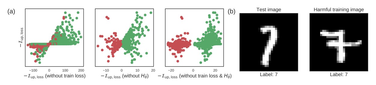
Figure 1. Components of influence. (a) What is the effect of the training loss and terms in ? Here, we plot against variants that are missing these terms and show that they are necessary for picking up the truly influential training points. For these calculations, we use logistic regression to distinguish 1’s from 7’s in MNIST (LeCun et al., 1998), picking an arbitrary test point ; similar trends hold across other test points. Green dots are train images of the same label as the test image (7) while red dots are 1’s. Left: Without the train loss term, we overestimate the influence of many training points: the points near the line should have close to 0, but instead have high influence when we remove the train loss term. Mid: Without , all green training points are helpful (removing each point increases test loss) and all red points are harmful (removing each point decreases test loss). This is because (all pixel values are positive), so , but it is incorrect: many harmful training points actually share the same label as . See panel (b). Right: Without training loss or , what is left is the scaled Euclidean inner product , which fails to accurately capture influence; the scatter plot deviates quite far from the diagonal. (b) The test image and a harmful training image with the same label. To the model, they look very different, so the presence of the training image makes the model think that the test image is less likely to be a 7. The Euclidean inner product does not pick up on these less intuitive, but important, harmful influences.
图 1. 影响的各个组成部分。(a) 里的训练损失项和 项起什么作用?这里把 与去掉这些项后的变体对照,说明它们对找出真正有影响的训练点是必要的。计算时,用逻辑回归在 MNIST(LeCun et al., 1998)上区分 1 和 7,并任取一个测试点 ;其他测试点上也有类似趋势。绿点是与测试图像标签相同(7)的训练图像,红点是 1。左:去掉训练损失项后,许多训练点的影响会被高估:靠近 线的点,其 本应接近 0,但去掉训练损失项后影响却很高。中:去掉 后,所有绿色训练点都变成有益的(去掉该点会增加测试损失),所有红点都变成有害的(去掉该点会降低测试损失)。这是因为 (所有像素值都为正),于是 ,但这一判断并不对:许多有害的训练点其实与 标签相同。见面板 (b)。右:既去掉训练损失又去掉 后,剩下的就是缩放后的欧氏内积 ,它无法准确刻画影响,散点会明显偏离对角线。(b) 测试图像,以及一张标签相同却有害的训练图像。在模型看来,它们差别很大,因此这张训练图像的存在会让模型觉得测试图像更不像是 7。欧氏内积捕捉不到这类不那么直观、却很重要的有害影响。
3. Efficiently Calculating Influence
3. 高效计算影响
There are two computational challenges to using . First, it requires forming and inverting , the Hessian of the empirical risk. With training points and , this requires operations, which is too expensive for models like deep neural networks with millions of parameters. Second, we often want to calculate across all training points .
使用 有两个计算上的难点。第一,需要形成并求逆经验风险的 Hessian 。有 个训练点且 时,这需要 次运算,对参数以百万计的深度网络来说太贵。第二,我们常常要对所有训练点 计算 。
The first problem is well-studied in second-order optimization. The idea is to avoid explicitly computing ; instead, we use implicit Hessian-vector products (HVPs) to efficiently approximate and then compute . This also solves the second problem: for each test point of interest, we can precompute and then efficiently compute for each training point .
第一个问题在二阶优化里已被充分研究。做法是避免显式计算 ;改为用隐式的 Hessian-向量积(HVP)高效近似 ,再计算 。这也解决了第二个问题:对每个感兴趣的测试点,可以预先算出 ,再对每个训练点 高效计算 。
We discuss two techniques for approximating , both relying on the fact that the HVP of a single term in , , can be computed for arbitrary in the same time that would take, which is typically (Pearlmutter, 1994).
下面讨论两种近似 的技术,它们都依赖于这样一个事实: 中单独一项的 HVP,,对任意 都可以在与计算 相同的时间内完成,通常是 (Pearlmutter, 1994)。
Conjugate gradients (CG).
共轭梯度(CG)。
The first technique is a standard transformation of matrix inversion into an optimization problem. Since by assumption, . We can solve this with CG approaches that only require the evaluation of , which takes time, without explicitly forming . While an exact solution takes CG iterations, in practice we can get a good approximation with fewer iterations; see Martens (2010) for more details.
第一种技术是把矩阵求逆标准地改写成优化问题。由于按假定 ,有 。可以用只需计算 的共轭梯度来求解,耗时 ,不必显式形成 。精确求解需要 次 CG 迭代,但实践中用更少的迭代就能得到很好的近似;细节见 Martens (2010)。
Stochastic estimation.
随机估计。
With large datasets, standard CG can be slow; each iteration still goes through all training points. We use a method developed by Agarwal et al. (2016) to get an estimator that only samples a single point per iteration, which results in significant speedups.
数据量大时,标准 CG 可能仍很慢:每次迭代还是要扫过全部 个训练点。我们采用 Agarwal et al. (2016) 提出的方法,得到每步只抽一个点的估计器,从而显著加速。
Dropping the subscript for clarity, let , the first terms in the Taylor expansion of . Rewrite this recursively as . From the validity of the Taylor expansion, as . The key is that at each iteration, we can substitute the full with a draw from any unbiased (and faster-to-compute) estimator of to form . Since , we still have .
为书写清楚,下面略去 下标。令 ,即 的 Taylor 展开的前 项。递归地写成 。由 Taylor 展开的成立性,当 时 。关键在于:每一步都可以把完整的 换成任何一个无偏(且算得更快)的估计,从而形成 。由于 ,仍然有 。
2 We assume w.l.o.g. that ; if this is not true, we can scale the loss down without affecting the parameters. In some cases, we can get an upper bound on (e.g., for linear models and bounded input), which makes this easy. Otherwise, we treat the scaling as a separate hyperparameter and tune it such that the Taylor expansion converges.
2 我们不失一般性地假定 ;若不成立,可以把损失缩小一个尺度而不影响参数。有些情况下可以得到 的上界(例如线性模型且输入有界),这件事就很容易。否则,把这个尺度当作单独的超参数,调到 Taylor 展开收敛为止。
In particular, we can uniformly sample and use as an unbiased estimator of . This gives us the following procedure: uniformly sample points from the training data; define ; and recursively compute , taking as our final unbiased estimate of . We pick to be large enough such that stabilizes, and to reduce variance we repeat this procedure times and average results. Empirically, we found this significantly faster than CG.
具体地,可以均匀抽取 ,并用 作为 的无偏估计。于是有如下步骤:从训练数据中均匀抽取 个点 ;定义 ;再递归计算 ,以 作为 的最终无偏估计。把 取得足够大,使 稳定;为降低方差,把这一过程重复 次再取平均。经验上,这比 CG 快得多。
We note that the original method of Agarwal et al. (2016) dealt only with generalized linear models, for which can be efficiently computed in time. In our case, we rely on Pearlmutter (1994)’s more general algorithm for fast HVPs, described above, to achieve the same time complexity.
需要说明,Agarwal et al. (2016) 的原方法只处理广义线性模型,在那种情况下 可以在 时间内高效计算。我们这里则依赖上面介绍的 Pearlmutter (1994) 更一般的快速 HVP 算法,达到同样的时间复杂度。
3 To increase stability, especially with non-convex models (see Section 4.2), we can also sample a mini-batch of training points at each iteration, instead of relying on a single training point.
3 为提高稳定性,尤其是对非凸模型(见第 4.2 节),每一步也可以抽取一小批训练点,而不是只依赖单个训练点。
With these techniques, we can compute on all training points in time; we show in Section 4.1 that empirically, choosing gives accurate results. Similarly, we compute with two matrix-vector products: we first compute , then , with the same HVP trick. These computations are easy to implement in auto-grad systems like TensorFlow (Abadi et al., 2015) and Theano (Theano D. Team, 2016), as users need only specify ; the rest is automatically handled.
有了这些技术,就可以在 时间内对所有训练点 计算 ;第 4.1 节将表明,经验上取 就能得到准确结果。类似地,计算 只需两次矩阵-向量积:先算 ,再算 ,用的是同一套 HVP 技巧。这些计算很容易在 TensorFlow(Abadi et al., 2015)和 Theano(Theano D. Team, 2016)这类自动求导系统里实现:用户只需指定 ,其余都自动完成。
4. Validation and Extensions
4. 验证与推广
Recall that influence functions are asymptotic approximations of leave-one-out retraining under the assumptions that (i) the model parameters minimize the empirical risk, and that (ii) the empirical risk is twice-differentiable and strictly convex. Here, we empirically show that influence functions are accurate approximations (Section 4.1) that provide useful information even when these assumptions are violated (Sections 4.2, 4.3).
回顾一下,影响函数是在如下假定下对留一法重训的渐近近似:(i) 模型参数 最小化经验风险;(ii) 经验风险二阶可微且严格凸。下面用实验表明,影响函数是准确的近似(第 4.1 节),即使这些假定被打破,它们仍能提供有用信息(第 4.2、4.3 节)。
4.1. Influence functions vs. leave-one-out retraining
4.1. 影响函数与留一法重训的对比
Influence functions assume that the weight on a training point is changed by an infinitesimally small . To investigate the accuracy of using influence functions to approximate the effect of removing a training point and retraining, we compared with (i.e., actually doing leave-one-out retraining). With a logistic regression model on 10-class MNIST, the predicted and actual changes matched closely (Fig 2-Left).
影响函数假定训练点上的权重只被改动一个无穷小的 。为考察用它来近似“去掉一个训练点再重训”的效果有多准,我们把 与 (也就是真正做留一法重训)相比较。在十类 MNIST 的逻辑回归上,预测变化与实际变化吻合得很紧密(图 2 左)。
4 We trained with L-BFGS (Liu & Nocedal, 1989), with regularization of 0.01, , and parameters.
4 我们用 L-BFGS(Liu & Nocedal, 1989)训练, 正则系数为 0.01,,参数个数 。
The stochastic approximation from Agarwal et al. (2016) was also accurate with repeats and iterations (Fig 2-Mid). Since each iteration only requires one HVP , this runs quickly: in fact, we accurately estimated without even looking at every data point, since . Surprisingly, even worked; while results were noisier, it was still able to identify the most influential points.
Agarwal et al. (2016) 的随机近似在重复 次、迭代 步时同样准确(图 2 中)。每步只需一次 HVP ,因此跑得很快:实际上,由于 ,我们甚至不必看遍每个数据点,就能准确估计 。出人意料的是,即便 也行;结果噪声更大,但仍能找出影响最大的那些点。
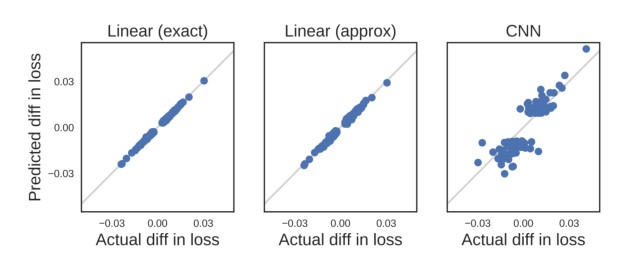
Figure 2. Influence matches leave-one-out retraining. We arbitrarily picked a wrongly-classified test point , but this trend held more broadly. These results are from 10-class MNIST. Left: For each of the 500 training points with largest , we plotted against the actual change in test loss after removing that point and retraining. The inverse HVP was solved exactly with CG. Mid: Same, but with the stochastic approximation. Right: The same plot for a CNN, computed on the 100 most influential points with CG. For the actual difference in loss, we removed each point and retrained from for 30k steps.
图 2. 影响与留一法重训相符。我们任意选取了一个被分错的测试点 ,但这一趋势更普遍地成立。结果来自十类 MNIST。左:对 最大的 500 个训练点 ,把 与去掉该点并重训后测试损失的实际变化相对照。逆 HVP 用 CG 精确求解。中:同样的图,但改用随机近似。右:卷积神经网络上的同样对照,用 CG 对影响最大的 100 个点计算。实际损失差的做法是:去掉每个点后,从 再训练 3 万步。
4.2. Non-convexity and non-convergence
4.2. 非凸与未收敛
In Section 2, we took as the global minimum. In practice, if we obtain our parameters by running SGD with early stopping or on non-convex objectives, . As a result, could have negative eigenvalues. We show that influence functions on still give meaningful results in practice.
第 2 节把 当作全局最小点。实践中,若参数 来自带提前停止的 SGD,或来自非凸目标,则 。结果是 可能有负特征值。我们表明,在 上计算的影响函数在实践中仍然有意义。
Our approach is to form a convex quadratic approximation of the loss around , i.e., . Here, is a damping term that we add if has negative eigenvalues; this corresponds to adding regularization on . We then calculate using . If is close to a local minimum, this is correlated with the result of taking a Newton step from after removing weight from (see appendix B).
我们的做法是在 附近对损失做凸的二次近似,即 。这里的 是阻尼项:若 有负特征值就加上它,相当于对 加上 正则。然后用 计算 。若 接近某个局部最小点,这与从 出发、在去掉 上 权重后再走一步牛顿法的结果相关(见附录 B)。
We checked the behavior of in a non-convergent, non-convex setting by training a convolutional neural network for 500k iterations. The model had not converged and was not PD, so we added a damping term with . Even in this difficult setting, the predicted and actual changes in loss were highly correlated (Pearson’s , Fig 2-Right).
我们在一个未收敛、非凸的设定里检查了 的表现:把卷积神经网络训练 50 万步。模型尚未收敛,且 不正定,于是加上 的阻尼。即便在这种困难设定下,预测的损失变化与实际变化仍然高度相关(Pearson 相关系数 ,图 2 右)。
5 The network had 7 sets of convolutional layers with non-linearities, modeled after the all-convolutional network from (Springenberg et al., 2014). For speed, we used 10% of the MNIST training set and only 2,616 parameters, since repeatedly retraining the network was expensive. Training was done with mini-batches of 500 examples and the Adam optimizer (Kingma & Ba, 2014). The model had not converged after 500k iterations; training it for another 500k iterations, using a full training pass for each iteration, reduced train loss from 0.14 to 0.12.
5 网络有 7 组带 非线性的卷积层,结构仿自 (Springenberg et al., 2014) 的全卷积网络。为了速度,我们只用了 MNIST 训练集的 10%,参数也只有 2,616 个,因为反复重训网络代价很高。训练使用大小为 500 的小批量,以及 Adam 优化器(Kingma & Ba, 2014)。50 万步后模型尚未收敛;再训 50 万步,且每步扫过整个训练集,训练损失从 0.14 降到 0.12。
4.3. Non-differentiable losses
4.3. 不可微损失
What happens when the derivatives of the loss, and , do not exist? In this section, we show that influence functions computed on smooth approximations to non-differentiable losses can predict the behavior of the original, non-differentiable loss under leave-one-out retraining. The robustness of this approximation suggests that we can train non-differentiable models and swap out non-differentiable components for smoothed versions for the purposes of calculating influence.
如果损失的导数 和 并不存在,会怎样?本节表明,在不可微损失的光滑近似上算出的影响函数,可以预测原始不可微损失在留一法重训下的行为。这一近似相当稳健,意味着我们可以先训练不可微模型,再在计算影响时把不可微的部分换成光滑版本。
To see this, we trained a linear SVM on the same 1s vs. 7s MNIST task in Section 2.3. This involves minimizing ; this simple piecewise linear function is similar to ReLUs, which cause non-differentiability in neural networks. We set the derivatives at the hinge to 0 and calculated . As one might expect, this was inaccurate (Fig 3b-Left): the second derivative carries no information about how close a support vector is to the hinge, so the quadratic approximation of is linear (up to regularization), which leads to overestimating the influence of .
为此,我们在第 2.3 节同一项 1 对 7 的 MNIST 任务上训练了线性 SVM。这涉及最小化 ;这一简单的分段线性函数与造成神经网络不可微的 ReLU 类似。我们把铰链处的导数设为 0,再计算 。正如所料,这样并不准确(图 3b 左):二阶导数并不包含支持向量 离铰链有多近的信息,于是 的二次近似(除正则外)其实是线性的,从而导致 高估 的影响。
For the purposes of calculating influence, we approximated with , which approaches the hinge loss as (Fig 3a). Using the same SVM weights as before, we found that calculating using closely matched the actual change due to retraining in the original (Pearson’s ; Fig 3b-Mid) and remained accurate over a wide range of (Fig 3b-Right).
为计算影响,我们用 来近似 ,当 时它趋近铰链损失(图 3a)。沿用前面得到的 SVM 权重,用 计算 ,与在原始 上重训后的实际变化吻合得很紧密(Pearson 相关系数 ;图 3b 中),并且在相当宽的 范围内仍然准确(图 3b 右)。
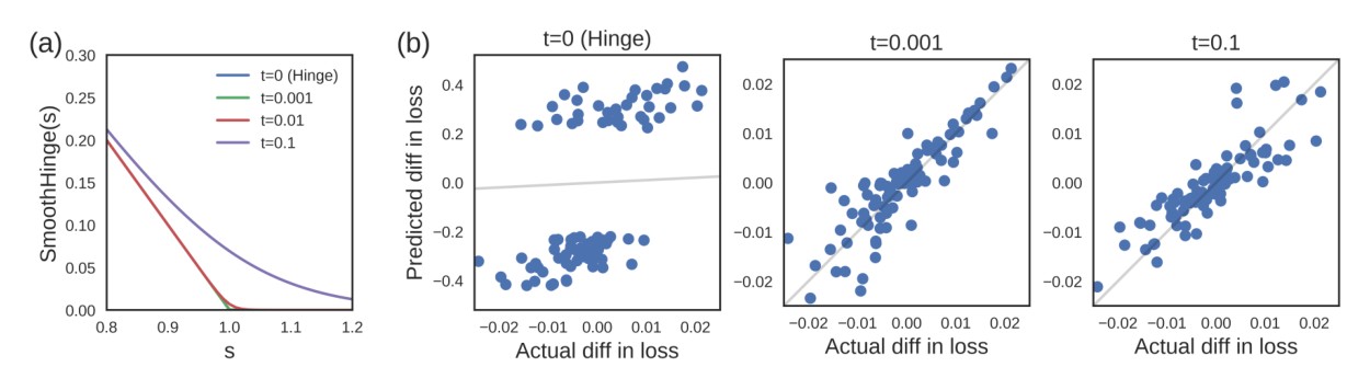
Figure 3. Smooth approximations to the hinge loss. (a) By varying , we can approximate the hinge loss with arbitrary accuracy: the green and blue lines are overlaid on top of each other. (b) Using a random, wrongly-classified test point, we compared the predicted vs. actual differences in loss after leave-one-out retraining on the 100 most influential training points. A similar trend held for other test points. The SVM objective is to minimize . Left: Influence functions were unable to accurately predict the change, overestimating its magnitude considerably. Mid: Using let us accurately predict the change in the hinge loss after retraining. Right: Correlation remained high over a wide range of , though it degrades when is too large. When , Pearson’s ; when , Pearson’s .
图 3. 铰链损失的光滑近似。(a) 通过改变 ,可以把铰链损失近似到任意精度:绿色与蓝色两条线叠在一起。(b) 任取一个被分错的测试点,在影响最大的 100 个训练点上,比较留一法重训后损失的预测变化与实际变化。其他测试点上也有类似趋势。SVM 的目标是最小化 。左:影响函数无法准确预测这一变化,明显高估了幅度。中:使用 后,可以准确预测重训后铰链损失的变化。右:在相当宽的 范围内相关性都保持很高,只是 过大时会下降。当 时,Pearson 相关系数 ;当 时,。
5. Use Cases of Influence Functions
5. 影响函数的用例
5.1. Understanding model behavior
5.1. 理解模型行为
By telling us the training points “responsible” for a given prediction, influence functions reveal insights about how models rely on and extrapolate from the training data. In this section, we show that two models can make the same correct predictions but get there in very different ways.
影响函数能指出对某次预测“该负责”的训练点,从而揭示模型怎样依赖训练数据、又怎样从中外推。本节表明,两个模型可以做出同样正确的预测,但走到这一结果的路径可以非常不同。
We compared (a) the state-of-the-art Inception v3 network (Szegedy et al., 2016) with all but the top layer frozen to (b) an SVM with an RBF kernel on a dog vs. fish image classification dataset we extracted from ImageNet (Russakovsky et al., 2015), with 900 training examples for each class. Freezing neural networks in this way is not uncommon in computer vision and is equivalent to training a logistic regression model on the bottleneck features (Donahue et al., 2014). We picked a test image both models got correct (Fig 4-Top) and used to compute the influence for the SVM.
我们比较了:(a) 当时最先进的 Inception v3 网络(Szegedy et al., 2016),除顶层外全部冻结;(b) 带 RBF 核的 SVM。任务是我们从 ImageNet(Russakovsky et al., 2015)抽出的狗对鱼图像分类,每类 900 个训练样本。在计算机视觉里这样冻结网络并不少见,等价于在瓶颈特征上训练逻辑回归(Donahue et al., 2014)。我们选了一张两个模型都分对的测试图像(图 4 上),并用 计算 SVM 的影响。
6 We used pre-trained weights from Keras (Chollet, 2015).
6 我们使用了 Keras(Chollet, 2015)中的预训练权重。
As expected, in the RBF SVM varied inversely with raw pixel distance, with training images far from the test image in pixel space having almost no influence. The Inception influences were much less correlated with distance in pixel space (Fig 4-Left). Looking at the two most helpful images (most positive ) for each model in Fig 4-Right, we see that the Inception network picked up on the distinctive characteristics of clownfish, whereas the RBF SVM pattern-matched training images superficially.
正如所料,RBF SVM 中的 与原始像素距离呈反向变化:像素空间里离测试图像很远的训练图像几乎没有影响。Inception 的影响与像素空间距离的相关性要低得多(图 4 左)。看图 4 右里两个模型各自最有帮助的两张图( 最正的那些),可以看到 Inception 网络抓住了小丑鱼的显著特征,而 RBF SVM 只是在表面上对训练图像做模式匹配。
Moreover, in the RBF SVM, fish (green points) close to the test image were mostly helpful, while dogs (red) were mostly harmful, with the RBF acting as a soft nearest neighbor function (Fig 4-Left). In contrast, in the Inception network, fish and dogs could be helpful or harmful for correctly classifying the test image as a fish; in fact, some of the most helpful training images were dogs that, to the model, looked very different from the test fish (Fig 4-Top).
此外,在 RBF SVM 中,靠近测试图像的鱼(绿点)大多是有益的,狗(红点)大多是有害的,RBF 此时表现得像一个软近邻函数(图 4 左)。相反,在 Inception 网络中,鱼和狗都既可能有益也可能有害于把测试图像正确分为鱼;事实上,一些最有帮助的训练图像是狗,在模型看来它们与测试中的鱼差别很大(图 4 上)。
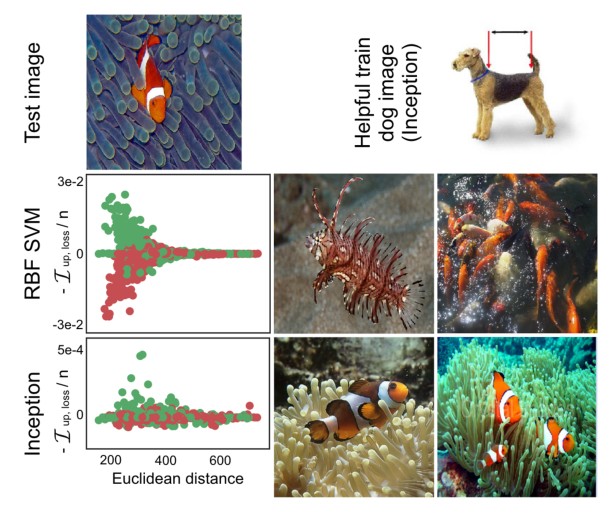
Figure 4. Inception vs. RBF SVM. Bottom left: vs. . Green dots are fish and red dots are dogs. Bottom right: The two most helpful training images, for each model, on the test. Top right: An image of a dog in the training set that helped the Inception model correctly classify the test image as a fish.
图 4. Inception 与 RBF SVM。左下: 对 。绿点是鱼,红点是狗。右下:对这张测试图,两个模型各自最有帮助的两张训练图像。右上:训练集中的一张狗,它帮助 Inception 模型把测试图像正确分为鱼。
5.2. Adversarial training examples
5.2. 对抗训练样本
In this section, we show that models that place a lot of influence on a small number of points can be vulnerable to training input perturbations, posing a serious security risk in real-world ML systems where attackers can influence the training data (Huang et al., 2011). Recent work has generated adversarial test images that are visually indistinguishable from real test images but completely fool a classifier (Goodfellow et al., 2015; Moosavi-Dezfooli et al., 2016). We demonstrate that influence functions can be used to craft adversarial training images that are similarly visually-indistinguishable and can flip a model’s prediction on a separate test image. To the best of our knowledge, this is the first proof-of-concept that visually-indistinguishable training attacks can be executed on otherwise highly-accurate neural networks.
本节表明,若模型把大量影响集中在少数点上,就可能容易受到训练输入扰动的攻击;在攻击者能够影响训练数据的真实机器学习系统里,这会带来严重的安全风险(Huang et al., 2011)。近期工作已经构造出与真实测试图像在视觉上难以分辨、却能完全愚弄分类器的对抗测试图像(Goodfellow et al., 2015; Moosavi-Dezfooli et al., 2016)。我们表明,影响函数也可以用来制作同样在视觉上难以分辨、并能翻转模型对另一张测试图像预测的对抗训练图像。据我们所知,这是在原本高度准确的神经网络上实施肉眼几乎分不出的训练集攻击的第一个概念验证。
The key idea is that tells us how to modify training point to most increase the loss on . Concretely, for a target test image , we can construct , an adversarial version of a training image , by initializing and then iterating , where is the step size and projects onto the set of valid images that share the same 8-bit representation with . After each iteration, we retrain the model. This is an iterated, training-set analogue of the methods used by, e.g., Goodfellow et al. (2015); Moosavi-Dezfooli et al. (2016) for test-set attacks.
关键在于: 告诉我们该怎样改训练点 ,才能最大幅度地增加 上的损失。具体地,对目标测试图像 ,可以从 出发,迭代 ,从而构造训练图像 的对抗版本 。其中 是步长, 把结果投影到与 具有相同 8 比特表示的合法图像集合上。每一步之后都重训模型。这是 Goodfellow et al. (2015)、Moosavi-Dezfooli et al. (2016) 等测试集攻击方法在训练集上的迭代对应物。
We tested these training attacks on the same Inception network on dogs vs. fish from Section 5.1, choosing this pair of animals to provide a stark contrast between the classes. We set and ran the attack for 100 iterations on each test image. As before, we froze all but the top layer for training; note that computing still involves differentiating through the entire network. Originally, the model correctly classified 591 / 600 test images. For each of these 591 test images, considered separately, we tried to find a visually-indistinguishable perturbation (i.e., same 8-bit representation) to a single training image, out of 1,800 total training images, that would flip the model’s prediction. We were able to do this on 335 (57%) of the 591 test images. By perturbing 2 training images for each test image, we could flip predictions on 77% of the 591 test images; and if we perturbed 10 training images, we could flip all but 1 of the 591. The above results are from attacking each test image separately, i.e., using a different training set to attack each test image. We also tried to attack multiple test images simultaneously by increasing their average loss, and found that single training image perturbations could simultaneously flip multiple test predictions as well (Fig 5).
我们在第 5.1 节同一套狗对鱼的 Inception 网络上测试了这些训练攻击,选择这一对动物是为了让两类形成鲜明对比。取 ,对每张测试图像攻击 100 步。和前面一样,训练时除顶层外全部冻结;但计算 仍需对整个网络求导。原先模型在 600 张测试图像中正确分类了 591 张。对这 591 张测试图像分别考虑,我们尝试在全部 1,800 张训练图像中,只对其中一张施加肉眼几乎分不出的扰动(即保持相同的 8 比特表示),使模型预测翻转。在 335 张(57%)测试图像上做成了这件事。若对每张测试图像扰动 2 张训练图像,可以翻转 591 张中的 77%;若扰动 10 张训练图像,591 张里只剩 1 张没被翻转。以上结果是对每张测试图像分开攻击,也就是用不同的训练集去打每一张测试图像。我们还尝试通过提高平均损失来同时攻击多张测试图像,发现对单张训练图像的扰动也可以同时翻转多个测试预测(图 5)。
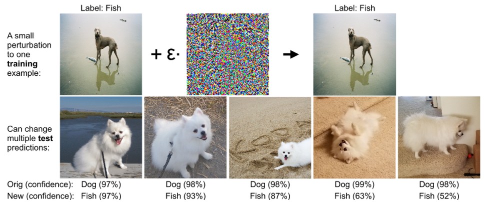
Figure 5. Training-set attacks. We targeted a set of 30 test images featuring the first author’s dog in a variety of poses and backgrounds. By maximizing the average loss over these 30 images, we created a visually-imperceptible change to the particular training image (shown on top) that flipped predictions on 16 test images.
图 5. 训练集攻击。我们瞄准一组 30 张测试图像,内容是第一作者的狗在不同姿态和背景下的照片。通过最大化这 30 张图上的平均损失,我们对特定训练图像(图上方所示)做了肉眼难以察觉的改动,从而翻转了其中 16 张测试图像的预测。
We make three observations about these attacks. First, though the change in pixel values is small, the change in the final Inception feature layer is significantly larger: using distance in pixel space, the training values change by less than 1% of the mean distance of a training point to its class centroid, whereas in Inception feature space, the change is on the same order as the mean distance. This leaves open the possibility that our attacks, while visually-imperceptible, can be detected by examining the feature space. Second, the attack tries to perturb the training example in a direction of low variance, causing the model to overfit in that direction and consequently incorrectly classify the test images; we expect attacking to be harder as the number of training examples grows. Third, ambiguous or mislabeled training images are effective points to attack: the model has low confidence and thus high loss on them, making them highly influential (recall Section 2.3). For example, the image in Fig 5 contains both a dog and a fish and is highly ambiguous; as a result, it is the training example that the model is least confident on (with a confidence of 77%, compared to the next lowest confidence of 90%).
关于这些攻击,我们有三点观察。第一,尽管像素值的改动很小,最后一层 Inception 特征上的变化却明显更大:用像素空间的 距离衡量,训练值的变化不到该点到其类中心平均距离的 1%;而在 Inception 特征空间里,变化与这一平均距离同一量级。因此,这些攻击虽然肉眼难以察觉,仍有可能通过检查特征空间被发现。第二,攻击试图沿低方差方向扰动训练样本,使模型在该方向上过拟合,进而把测试图像分错;随着训练样本增多,攻击应当会更难。第三,含糊或标错的训练图像是有效的攻击点:模型对它们置信度低、损失高,因而影响很大(回顾第 2.3 节)。例如,图 5 中的图像同时含有狗和鱼,非常含糊;结果它成了模型置信度最低的训练样本(置信度为 77%,下一项最低的也有 90%)。
This attack is mathematically equivalent to the gradient-based training set attacks explored by Biggio et al. (2012); Mei & Zhu (2015b) and others in the context of different models. Biggio et al. (2012) constructed a dataset poisoning attack against a linear SVM on a two-class MNIST task, but had to modify the training points in an obviously distinguishable way to be effective. Measuring the magnitude of gives model developers a way of quantifying how vulnerable their models are to training-set attacks.
这一攻击在数学上等价于 Biggio et al. (2012)、Mei & Zhu (2015b) 等在不同模型背景下探讨过的、基于梯度的训练集攻击。Biggio et al. (2012) 曾在两类 MNIST 任务上对线性 SVM 构造数据投毒攻击,但要使攻击有效,必须把训练点改到一眼就能看出差别。测量 的大小,给模型开发者提供了一种量化模型对训练集攻击有多脆弱的方法。
5.3. Debugging domain mismatch
5.3. 调试域不匹配
Domain mismatch — where the training distribution does not match the test distribution — can cause models with high training accuracy to do poorly on test data (Ben-David et al., 2010). We show that influence functions can identify the training examples most responsible for the errors, helping model developers identify domain mismatch.
域不匹配——训练分布与测试分布不一致——会让训练准确率很高的模型在测试数据上表现很差(Ben-David et al., 2010)。我们表明,影响函数可以找出对这些错误最该负责的训练样本,帮助模型开发者识别域不匹配。
As a case study, we predicted whether a patient would be readmitted to hospital. Domain mismatches are common in biomedical data, e.g., different hospitals serve different populations, and models trained on one population can do poorly on another (Kansagara et al., 2011). We used logistic regression to predict readmission with a balanced training dataset of 20K diabetic patients from 100+ US hospitals, each represented by 127 features (Strack et al., 2014).
作为案例,我们预测患者是否会再次入院。生物医学数据里域不匹配很常见,例如不同医院服务的人群不同,在一个人群上训练的模型到另一个人群上可能表现很差(Kansagara et al., 2011)。我们用逻辑回归预测再入院,训练数据是来自美国 100 多家医院、经过均衡的 2 万名糖尿病患者,每人用 127 个特征表示(Strack et al., 2014)。
7 Hospital readmission was defined as whether a patient would be readmitted within the next 30 days. Features were demographic (e.g., age, race, gender), administrative (e.g., length of hospital stay), or medical (e.g., test results).
7 再入院定义为患者是否会在接下来 30 天内再次入院。特征分为人口学特征(例如年龄、种族、性别)、行政特征(例如住院天数)或医学特征(例如化验结果)。
3 out of the 24 children under age 10 in this dataset were re-admitted. To induce a domain mismatch, we filtered out 20 children who were not re-admitted, leaving 3 out of 4 re-admitted. This caused the model to wrongly classify many children in the test set. Our aim is to identify the 4 children in the training set as being “responsible” for these errors.
该数据集中 24 名 10 岁以下儿童里,有 3 名再次入院。为制造域不匹配,我们滤掉了 20 名未再入院的儿童,剩下 4 人中有 3 人再入院。这导致模型把测试集里的许多儿童分错。我们的目标是把训练集中这 4 名儿童识别为对这些错误“该负责”的样本。
As a baseline, we tried the common practice of looking at the learned parameters to see if the indicator variable for being a child was obviously different. However, this did not work: 14/127 features had a larger coefficient.
作为基线,我们试了常见做法:查看学到的参数 ,看“是否为儿童”这一指示变量是否明显与众不同。但这并不奏效:127 个特征里有 14 个的系数更大。
Picking a random child that the model got wrong, we calculated for each training point . This clearly highlighted the 4 training children, each of whom were 30-40 times as influential as the next most influential examples. The 1 child in the training set who was not readmitted had a very positive influence, while the other 3 had very negative influences. Moreover, calculating on these 4 children showed that the ‘child’ indicator variable contributed significantly to the magnitude of .
我们任取一个模型分错的儿童 ,对每个训练点 计算 。这清楚地标出了训练集中的 4 名儿童,他们每人的影响都是下一批最有影响样本的 30 到 40 倍。训练集里那 1 名未再入院的儿童影响非常正,另外 3 名则非常负。此外,在这 4 名儿童上计算 表明,“是否为儿童”这一指示变量对 的幅度贡献很大。
5.4. Fixing mislabeled examples
5.4. 修正标错的样本
Labels in the real world are often noisy, especially if crowdsourced (Frénay & Verleysen, 2014), and can even be adversarially corrupted. Even if a human expert could recognize wrongly labeled examples, it is impossible in many applications to manually review all of the training data. We show that influence functions can help human experts prioritize their attention, allowing them to inspect only the examples that actually matter.
现实世界里的标签常常有噪声,众包时尤其如此(Frénay & Verleysen, 2014),甚至可能被对抗性地篡改。即便人类专家能够认出标错的样本,在许多应用里也不可能手工审完全部训练数据。我们表明,影响函数可以帮助专家把注意力排好优先次序,从而只检查真正要紧的样本。
The key idea is to flag the training points that exert the most influence on the model. Because we do not have access to the test set, we measure the influence of with , which approximates the error incurred on if we remove from the training set.
关键想法是标出对模型影响最大的那些训练点。由于没有测试集,我们用 来衡量 的影响,它近似的是:若把 从训练集中去掉,会在 上造成多大误差。
Our case study is email spam classification, which relies on user-provided labels and is also vulnerable to adversarial attack (Biggio et al., 2011). We flipped the labels of a random 10% of the training data and then simulated manually inspecting a fraction of the training points, correcting them if they had been flipped. Using influence functions to prioritize the training points to inspect allowed us to repair the dataset (Fig 6, blue) without checking too many points, outperforming the baselines of checking points with the highest train loss (Fig 6, green) or at random (Fig 6, red). No method had access to the test data.
案例是电子邮件垃圾分类:它依赖用户提供的标签,也容易受到对抗攻击(Biggio et al., 2011)。我们随机翻转了 10% 训练数据的标签,然后模拟人工检查一部分训练点,若被翻转过就改回来。用影响函数来决定先检查哪些训练点,使我们不必检查太多点就能把数据集修好(图 6,蓝线),效果好于先检查训练损失最高的点(图 6,绿线)或随机检查(图 6,红线)。这些方法都没有使用测试数据。
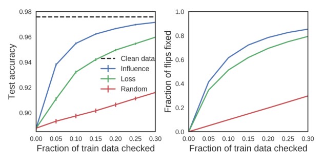
Figure 6. Fixing mislabeled examples. Plots of how test accuracy (left) and the fraction of flipped data detected (right) change with the fraction of train data checked, using different algorithms for picking points to check. Error bars show the std. dev. across 40 repeats of this experiment, with a different subset of labels flipped in each; error bars on the right are too small to be seen. These results are on the Enron1 spam dataset (Metsis et al., 2006), with 4,147 training and 1,035 test examples; we trained logistic regression on a bag-of-words representation of the emails.
图 6. 修正标错的样本。左图是测试准确率、右图是被检出的翻转数据比例,随被检查的训练数据比例如何变化;不同算法用于选择要检查的点。误差条给出该实验重复 40 次的标准差,每次翻转的标签子集不同;右图的误差条小到几乎看不见。结果来自 Enron1 垃圾邮件数据集(Metsis et al., 2006),有 4,147 个训练样本和 1,035 个测试样本;我们在邮件的词袋表示上训练逻辑回归。
6. Related Work
6. 相关工作
The use of influence-based diagnostics originated in statistics in the 70s and 80s, driven by seminal papers by Cook and others (Cook, 1977; Cook & Weisberg, 1980; 1982), though similar ideas appeared even earlier in other forms, e.g., the infinitesimal jackknife (Jaeckel, 1972). Earlier work focused on removing training points from linear models, with later work extending this to more general models and a wider variety of perturbations (Cook, 1986; Thomas & Cook, 1990; Chatterjee & Hadi, 1986; Wei et al., 1998). Most of this prior work focused on experiments with small datasets, e.g., and in Cook & Weisberg (1980), with special attention therefore paid to exact solutions, or if not possible, characterizations of the error terms.
基于影响的诊断方法起源于 20 世纪七八十年代的统计学,由 Cook 等人的开创性论文推动(Cook, 1977; Cook & Weisberg, 1980; 1982),不过类似想法更早已以其他形式出现,例如无穷小刀切法(Jaeckel, 1972)。早期工作主要关注从线性模型中去掉训练点,后来的工作把它推广到更一般的模型和更多种类的扰动(Cook, 1986; Thomas & Cook, 1990; Chatterjee & Hadi, 1986; Wei et al., 1998)。这些先前工作大多在小数据集上做实验,例如 Cook & Weisberg (1980) 中 、,因此特别重视精确解,或在无法精确求解时刻画误差项。
Influence functions have not been used much in the ML literature, with some exceptions. Christmann & Steinwart (2004); Debruyne et al. (2008); Liu et al. (2014) use influence functions to study model robustness and to do fast cross-validation in kernel methods. Wojnowicz et al. (2016) uses matrix sketching to estimate Cook’s distance, which is closely related to influence; they focus on prioritizing training points for human attention and derive methods specific to generalized linear models.
影响函数在机器学习文献里用得还不多,不过也有例外。Christmann & Steinwart (2004)、Debruyne et al. (2008)、Liu et al. (2014) 用影响函数研究模型稳健性,并在核方法中做快速交叉验证。Wojnowicz et al. (2016) 用矩阵素描来估计与影响密切相关的 Cook 距离;他们关注的是为人工检查排定训练点的优先次序,并推导了适用于广义线性模型的方法。
As noted in Section 5.2, our training-set attack is mathematically equivalent to an approach first explored by Biggio et al. (2012) in the context of SVMs, with follow-up work extending the framework and applying it to linear and logistic regression (Mei & Zhu, 2015b), topic modeling (Mei & Zhu, 2015a), and collaborative filtering (Li et al., 2016a). These papers derived the attack directly from the KKT conditions without considering influence, though for continuous data, the end result is equivalent. Influence functions additionally let us consider attacks on discrete data (Section 2.2), but we have not tested this empirically. Our work connects the literature on training-set attacks with work on “adversarial examples” (Goodfellow et al., 2015; Moosavi-Dezfooli et al., 2016), visually-imperceptible perturbations on test inputs.
如第 5.2 节所述,我们的训练集攻击在数学上等价于 Biggio et al. (2012) 最先在 SVM 背景下探讨的方法,后续工作把这一框架推广并应用到线性与逻辑回归(Mei & Zhu, 2015b)、主题模型(Mei & Zhu, 2015a)以及协同过滤(Li et al., 2016a)。这些论文直接从 KKT 条件导出攻击,并没有考虑影响;不过对连续数据,最终结果是等价的。影响函数还让我们可以考虑对离散数据的攻击(第 2.2 节),但我们尚未对此做实证检验。本文把关于训练集攻击的文献,与关于测试输入上肉眼难以察觉扰动的“对抗样本”工作(Goodfellow et al., 2015; Moosavi-Dezfooli et al., 2016)连接起来。
In contrast to training-set attacks, Cadamuro et al. (2016) consider the task of taking an incorrect test prediction and finding a small subset of training data such that changing the labels on this subset makes the prediction correct. They provide a solution for OLS and Gaussian process models when the labels are continuous. Our work with influence functions allow us to solve this problem in a much larger range of models and in datasets with discrete labels.
与训练集攻击相对,Cadamuro et al. (2016) 考虑的是:面对一次错误的测试预测,找出一小撮训练数据,改掉这撮数据的标签就能让预测变对。他们为标签连续时的普通最小二乘和高斯过程模型给出了解法。我们借助影响函数,可以在更大范围的模型上、以及标签离散的数据集上解决这个问题。
7. Discussion
7. 讨论
We have discussed a variety of applications, from creating training-set attacks to debugging models and fixing datasets. Underlying each of these applications is a common tool, the influence function, which is based on a simple idea — we can better understand model behavior by looking at how it was derived from its training data.
我们讨论了多种应用,从构造训练集攻击,到调试模型和修正数据集。这些应用背后是同一种工具——影响函数,它基于一个简单想法:看模型怎样从训练数据中被推导出来,就能更好地理解它的行为。
At their core, influence functions measure the effect of local changes: what happens when we upweight a point by an infinitesimally-small ? This locality allows us to derive efficient closed-form estimates, and as we show, they can be surprisingly effective. However, we might want to ask about more global changes, e.g., how does a subpopulation of patients from this hospital affect the model? Since influence functions depend on the model not changing too much, how to tackle this is an open question.
从根本上说,影响函数衡量的是局部变化的效果:把一个点的权重上调一个无穷小的 ,会发生什么?这种局部性让我们可以导出高效的闭式估计,而且如我们所示,它们可以出奇地有效。不过,我们也许还想问更全局的变化,例如来自这家医院的一群患者会怎样影响模型?影响函数依赖于模型不会变化太大,如何处理这一问题仍是开放的。
It seems inevitable that high-performing, complex, black-box models will become increasingly prevalent and important. We hope that the approach presented here — of looking at the model through the lens of the training data — will become a standard part of the toolkit of developing, understanding, and diagnosing machine learning.
高性能、复杂的黑盒模型会越来越普遍、也越来越重要,这似乎不可避免。我们希望本文给出的做法——透过训练数据来看模型——会成为开发、理解和诊断机器学习的一套标准工具。
The code and data for replicating our experiments is available on GitHub http://bit.ly/gt-influence and Codalab http://bit.ly/cl-influence.
复现实验的代码与数据可在 GitHub http://bit.ly/gt-influence 和 Codalab http://bit.ly/cl-influence 上获得。
Acknowledgements
致谢
We thank Jacob Steinhardt, Zhenghao Chen, and Hongseok Namkoong for helpful discussions and comments. This work was supported by a Future of Life Research Award and a Microsoft Research Faculty Fellowship.
感谢 Jacob Steinhardt、Zhenghao Chen 和 Hongseok Namkoong 的讨论与意见。本工作得到 Future of Life Research Award 以及 Microsoft Research Faculty Fellowship 的资助。
References
参考文献
Abadi, M., Agarwal, A., Barham, P., Brevdo, E., Chen, Z., Citro, C., Corrado, G. S., Davis, A., Dean, J., Devin, M., Ghemawat, S., Goodfellow, I. J., Harp, A., Irving, G., Isard, M., Jia, Y., Józefowicz, R., Kaiser, L., Kudlur, M., Levenberg, J., Mané, D., Monga, R., Moore, S., Murray, D. G., Olah, C., Schuster, M., Shlens, J., Steiner, B., Sutskever, I., Talwar, K., Tucker, P. A., Vanhoucke, V., Vasudevan, V., Viégas, F. B., Vinyals, O., Warden, P., Wattenberg, M., Wicke, M., Yu, Y., and Zheng, X. Tensorflow: Large-scale machine learning on heterogeneous distributed systems. arXiv preprint arXiv:1603.04467, 2015.
Adler, P., Falk, C., Friedler, S. A., Rybeck, G., Scheidegger, C., Smith, B., and Venkatasubramanian, S. Auditing black-box models for indirect influence. arXiv preprint arXiv:1602.07043, 2016.
Agarwal, N., Bullins, B., and Hazan, E. Second order stochastic optimization in linear time. arXiv preprint arXiv:1602.03943, 2016.
Amershi, S., Chickering, M., Drucker, S. M., Lee, B., Simard, P., and Suh, J. Modeltracker: Redesigning performance analysis tools for machine learning. In Conference on Human Factors in Computing Systems (CHI), pp. 337–346, 2015.
Ben-David, S., Blitzer, J., Crammer, K., Kulesza, A., Pereira, F., and Vaughan, J. W. A theory of learning from different domains. Machine Learning, 79(1):151–175, 2010.
Biggio, B., Nelson, B., and Laskov, P. Support vector machines under adversarial label noise. ACML, 20:97–112, 2011.
Biggio, B., Nelson, B., and Laskov, P. Poisoning attacks against support vector machines. In International Conference on Machine Learning (ICML), pp. 1467–1474, 2012.
Cadamuro, G., Gilad-Bachrach, R., and Zhu, X. Debugging machine learning models. In ICML Workshop on Reliable Machine Learning in the Wild, 2016.
Chatterjee, S. and Hadi, A. S. Influential observations, high leverage points, and outliers in linear regression. Statistical Science, pp. 379–393, 1986.
Chollet, F. Keras, 2015.
Christmann, A. and Steinwart, I. On robustness properties of convex risk minimization methods for pattern recognition. Journal of Machine Learning Research (JMLR), 5(0):1007–1034, 2004.
Cook, R. D. Detection of influential observation in linear regression. Technometrics, 19:15–18, 1977.
Cook, R. D. Assessment of local influence. Journal of the Royal Statistical Society. Series B (Methodological), pp. 133–169, 1986.
Cook, R. D. and Weisberg, S. Characterizations of an empirical influence function for detecting influential cases in regression. Technometrics, 22:495–508, 1980.
Cook, R. D. and Weisberg, S. Residuals and influence in regression. New York: Chapman and Hall, 1982.
Datta, A., Sen, S., and Zick, Y. Algorithmic transparency via quantitative input influence: Theory and experiments with learning systems. In Security and Privacy (SP), 2016 IEEE Symposium on, pp. 598–617, 2016.
Debruyne, M., Hubert, M., and Suykens, J. A. Model selection in kernel based regression using the influence function. Journal of Machine Learning Research (JMLR), 9(0):2377–2400, 2008.
Donahue, J., Jia, Y., Vinyals, O., Hoffman, J., Zhang, N., Tzeng, E., and Darrell, T. Decaf: A deep convolutional activation feature for generic visual recognition. In International Conference on Machine Learning (ICML), volume 32, pp. 647–655, 2014.
Frénay, B. and Verleysen, M. Classification in the presence of label noise: a survey. IEEE Transactions on Neural Networks and Learning Systems, 25:845–869, 2014.
Goodfellow, I. J., Shlens, J., and Szegedy, C. Explaining and harnessing adversarial examples. In International Conference on Learning Representations (ICLR), 2015.
Goodman, B. and Flaxman, S. European union regulations on algorithmic decision-making and a “right to explanation”. arXiv preprint arXiv:1606.08813, 2016.
Huang, L., Joseph, A. D., Nelson, B., Rubinstein, B. I., and Tygar, J. Adversarial machine learning. In Proceedings of the 4th ACM workshop on Security and artificial intelligence, pp. 43–58, 2011.
Jaeckel, L. A. The infinitesimal jackknife. Unpublished memorandum, Bell Telephone Laboratories, Murray Hill, NJ, 1972.
Kansagara, D., Englander, H., Salanitro, A., Kagen, D., Theobald, C., Freeman, M., and Kripalani, S. Risk prediction models for hospital readmission: a systematic review. JAMA, 306(15):1688–1698, 2011.
Kingma, D. and Ba, J. Adam: A method for stochastic optimization. arXiv preprint arXiv:1412.6980, 2014.
Krizhevsky, A., Sutskever, I., and Hinton, G. E. Imagenet classification with deep convolutional neural networks. In Advances in Neural Information Processing Systems (NIPS), pp. 1097–1105, 2012.
LeCun, Y., Bottou, L., Bengio, Y., and Haffner, P. Gradient-based learning applied to document recognition. Proceedings of the IEEE, 86(11):2278–2324, 1998.
Li, B., Wang, Y., Singh, A., and Vorobeychik, Y. Data poisoning attacks on factorization-based collaborative filtering. In Advances in Neural Information Processing Systems (NIPS), 2016a.
Li, J., Monroe, W., and Jurafsky, D. Understanding neural networks through representation erasure. arXiv preprint arXiv:1612.08220, 2016b.
Liu, D. C. and Nocedal, J. On the limited memory BFGS method for large scale optimization. Mathematical Programming, 45(1):503–528, 1989.
Liu, Y., Jiang, S., and Liao, S. Efficient approximation of cross-validation for kernel methods using Bouligand influence function. In International Conference on Machine Learning (ICML), pp. 324–332, 2014.
Martens, J. Deep learning via hessian-free optimization. In International Conference on Machine Learning (ICML), pp. 735–742, 2010.
Mei, S. and Zhu, X. The security of latent Dirichlet allocation. In Artificial Intelligence and Statistics (AISTATS), 2015a.
Mei, S. and Zhu, X. Using machine teaching to identify optimal training-set attacks on machine learners. In Association for the Advancement of Artificial Intelligence (AAAI), 2015b.
Metsis, V., Androutsopoulos, I., and Paliouras, G. Spam filtering with naive Bayes – which naive Bayes? In CEAS, volume 17, pp. 28–69, 2006.
Moosavi-Dezfooli, S., Fawzi, A., and Frossard, P. Deepfool: a simple and accurate method to fool deep neural networks. In Computer Vision and Pattern Recognition (CVPR), pp. 2574–2582, 2016.
Pearlmutter, B. A. Fast exact multiplication by the hessian. Neural Computation, 6(1):147–160, 1994.
Ribeiro, M. T., Singh, S., and Guestrin, C. “why should I trust you?”: Explaining the predictions of any classifier. In International Conference on Knowledge Discovery and Data Mining (KDD), 2016.
Russakovsky, O., Deng, J., Su, H., Krause, J., Satheesh, S., Ma, S., Huang, Z., Karpathy, A., Khosla, A., Bernstein, M., et al. ImageNet large scale visual recognition challenge. International Journal of Computer Vision, 115(3):211–252, 2015.
Shrikumar, A., Greenside, P., Shcherbina, A., and Kundaje, A. Not just a black box: Learning important features through propagating activation differences. arXiv preprint arXiv:1605.01713, 2016.
Simonyan, K., Vedaldi, A., and Zisserman, A. Deep inside convolutional networks: Visualising image classification models and saliency maps. arXiv preprint arXiv:1312.6034, 2013.
Springenberg, J. T., Dosovitskiy, A., Brox, T., and Riedmiller, M. Striving for simplicity: The all convolutional net. arXiv preprint arXiv:1412.6806, 2014.
Strack, B., DeShazo, J. P., Gennings, C., Olmo, J. L., Ventura, S., Cios, K. J., and Clore, J. N. Impact of HbA1c measurement on hospital readmission rates: analysis of 70,000 clinical database patient records. BioMed Research International, 2014, 2014.
Szegedy, C., Vanhoucke, V., Ioffe, S., Shlens, J., and Wojna, Z. Rethinking the Inception architecture for computer vision. In Computer Vision and Pattern Recognition (CVPR), pp. 2818–2826, 2016.
Theano D. Team. Theano: A Python framework for fast computation of mathematical expressions. arXiv preprint arXiv:1605.02688, 2016.
Thomas, W. and Cook, R. D. Assessing influence on predictions from generalized linear models. Technometrics, 32(1):59–65, 1990.
Wei, B., Hu, Y., and Fung, W. Generalized leverage and its applications. Scandinavian Journal of Statistics, 25:25–37, 1998.
Wojnowicz, M., Cruz, B., Zhao, X., Wallace, B., Wolff, M., Luan, J., and Crable, C. “Influence sketching”: Finding influential samples in large-scale regressions. arXiv preprint arXiv:1611.05923, 2016.