Infini-gram mini: Exact n-gram Search at the Internet Scale with FM-Index

Infini-gram mini：用 FM-Index 在互联网规模做精确 n-gram 检索

Hao Xu ♡   Jiacheng Liu ♡ ♠   Yejin Choi ♢   Noah A. Smith ♡ ♠   Hannaneh Hajishirzi ♡ ♠ Affiliation:  ♡ Paul G. Allen School of Computer Science & Engineering, University of Washington Affiliation:  ♠ Allen Institute for AI    ♢ Stanford University

Abstract

摘要

Language models are trained mainly on massive text data from the Internet, and it becomes increasingly important to understand this data source. Exact-match search engines enable searching in large text corpora – counting string appearances and retrieving the enclosing documents – yet the high storage overhead hinders their application on Internet-scale data. We present infini-gram mini, an efficient and scalable system that can make petabyte-level text corpora searchable. Based on the FM-index data structure (Ferragina and Manzini 2000), which simultaneously indexes and compresses text, our system creates indexes with size only 44% of the corpus. Infini-gram mini greatly improves upon the best existing implementation of FM-index in terms of indexing speed (18$\times$) and memory use during both indexing (3.2$\times$ reduction) and querying (down to a negligible amount). We index 46TB of Internet text in 50 days with a single CPU node with 128 vCPUs (or 19 hours if using 75 such nodes). We show one important use case of infini-gram mini in a large-scale analysis of benchmark contamination. We find several core LM evaluation benchmarks to be heavily contaminated in Internet crawls (up to 40% in SQuAD), which could lead to overestimating the capabilities of language models if trained on such data. We host a benchmark contamination bulletin to share the contamination rate of many core and community-contributed benchmarks. We also release a web interface and an API endpoint to serve general search queries on infini-gram mini indexes.

语言模型主要在海量互联网文本上训练，理解这一数据源愈发重要。精确匹配搜索引擎可在大规模语料中计数字符串出现并取回包围文档，但存储开销大，难用于互联网规模数据。我们提出 infini-gram mini：高效可扩展、能使拍字节级文本可检索的系统。基于同时索引与压缩文本的 FM-index（Ferragina and Manzini 2000），索引体积仅约语料的 44%。相对现有最佳 FM-index 实现，索引速度提升 18$\times$，索引期内存降 3.2$\times$，查询期内存可降至可忽略。我们在单台 128 vCPU 的 CPU 节点上用 50 天为 46TB 互联网文本建索引（若用 75 台同类节点约 19 小时）。重要用例是大规模基准污染分析：若干核心 LM 评测基准在互联网爬取中重度污染（SQuAD 可达 40%），若在其上训练会高估模型能力。我们托管污染公告板共享核心与社区基准的污染率，并发布 Web 界面与 API 端点服务检索。

	Project Home	infini-gram-mini.io
	Web Interface	infini-gram-mini.io/demo
	API Endpoint	api.infini-gram-mini.io
	Documentation	infini-gram-mini.io/docs
	Source Code	infini-gram-mini.io/code
	Contam Bulletin	infini-gram-mini.io/bulletin

	项目主页	infini-gram-mini.io
	Web 界面	infini-gram-mini.io/demo
	API 端点	api.infini-gram-mini.io
	文档	infini-gram-mini.io/docs
	源码	infini-gram-mini.io/code
	污染公告板	infini-gram-mini.io/bulletin

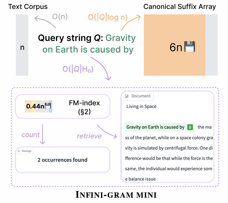
Figure 1: Overview of infini-gram mini. Based on the FM-index data structure, infini-gram mini supports efficient exact-match search in massive text corpora ($n=O(10^{15})$ bytes) while reducing the index size down to 7% compared to a canonical suffix array index. Searching naively in the corpus would have time complexity linear to $n$ and thus impractical; with infini-gram mini, the search time complexity is independent of $n$. $|Q|$ is the length of query string and can be arbitrarily long, and $H_{0}\approx 2.1$ is the zeroth-order entropy of the text corpus.

图 1：infini-gram mini 概览。基于 FM-index，可在海量语料（$n=O(10^{15})$ 字节）上高效精确匹配检索，索引体积相对经典后缀数组降至约 7%。朴素检索时间与 $n$ 线性相关、不现实；用 infini-gram mini 后检索复杂度与 $n$ 无关。$|Q|$ 为查询串长度可任意长，$H_{0}\approx 2.1$ 为语料零阶熵。

1 Introduction

1 引言

Modern language models (LMs) are trained mainly on text datasets downsampled from massive, petabyte-level text corpora like Common Crawl (Common Crawl Foundation 2025). As these LMs are deployed more broadly, it becomes more pressing to understand the training data and its effects on model behavior (Liu et al. 2025; Han and Tsvetkov 2022). As a starting point, we want to make these text corpora searchable; in particular, searching for exact matches of long sequences has gained increasing interest (Elazar et al. 2024; Merrill et al. 2024; Lu et al. 2024). The size of these corpora makes this problem extremely challenging, creating demand for more efficient indexing techniques.

现代语言模型（LM）主要训练于从 Common Crawl（Common Crawl Foundation 2025）等拍字节级语料下采样的文本。随部署面扩大，理解训练数据及其对模型行为的影响更迫切（Liu 等 2025；Han and Tsvetkov 2022）。起点是让这些语料可检索；对长序列做精确匹配检索兴趣日增（Elazar 等 2024；Merrill 等 2024；Lu 等 2024）。语料规模使问题极难，需要更高效的索引技术。

Prior systems for exact-match search build indexes several times as large as the text corpora. Merrill et al. 2024 indexes 1.3TB of text with suffix automaton (storage multiplier 29$\times$); Liu et al. 2024 indexes 12TB of text with suffix array (storage multiplier 6$\times$); Elazar et al. 2024 indexes 35TB of text with the proprietary ElasticSearch engine (storage multiplier about $2\times$). The size of these indexes renders it impractical to apply them to petabyte-level corpora.

先前精确匹配系统建的索引往往数倍于语料本身。Merrill 等 2024 用后缀自动机索引 1.3TB（存储倍率 29$\times$）；Liu 等 2024 用后缀数组索引 12TB（6$\times$）；Elazar 等 2024 用专有 ElasticSearch 索引 35TB（约 2$\times$）。索引体积使拍字节级应用不现实。

To address this challenge, we index text corpora with FM-index (Ferragina and Manzini 2000), a compact data structure frequently used in bioinformatics (Simpson and Durbin 2010; Li 2014; Wang et al. 2018), but not yet used for natural language data at scale. We explain FM-index in detail in §2. Compared to the canonical suffix array, FM-index only stores a subsampled version of the suffix array and a compressed version of the text corpus; the full version can be partially recovered at query time as needed. In other words, FM-index trades runtime compute for storage efficiency. For natural text, the size of FM-index can be made as small as 0.26$\times$ of the corpus; practically, to ensure low query latency, we build FM-index with a storage multiplier of 0.44$\times$, or 7% compared to the canonical suffix array.

为此，我们用 FM-index（Ferragina and Manzini 2000）索引文本语料——该紧凑结构在生物信息学常用（Simpson and Durbin 2010；Li 2014；Wang 等 2018），尚未大规模用于自然语言。§2 详述。相对经典后缀数组，FM-index 只存子采样后缀数组与压缩语料，完整版本可在查询时按需部分恢复，即以运行时算力换存储。对自然文本，体积可低至语料的 0.26$\times$；实践上为保低延迟，我们建 0.44$\times$ 倍率索引，约为经典后缀数组的 7%。

Infini-gram mini is the system we developed for efficiently constructing FM-index at scale and answering search queries. For indexing, we extend and combine components from Liu et al. 2024, Gog et al. 2014, and Labeit et al. 2017 into a highly parallelized program, which achieves a 18$\times$ speedup and uses only 32% as much RAM compared to the best existing implementation by SDSL (Gog et al. 2014).[^1] We use infini-gram mini to construct FM-index for two LM pretraining datasets – the Pile and DCLM-baseline – and three recent Common Crawl dumps between January and March 2025. Altogether, we indexed 46TB of text in 50 days with a single CPU node with 128 vCPUs, and this could have been done in 19 hours if embarrassingly parallelized across 75 such nodes. We estimate that indexing the full Common Crawl would take 1,200 node-days, or 19 hours if parallelized across 1,500 nodes. For answering queries, we extend SDSL to work with on-disk index, reducing the RAM requirement to a negligible amount. Our inference engine supports counting the occurrences of a query string and retrieving documents that contain the query string, both within seconds when working on the above corpora.

Infini-gram mini 是我们开发的系统：高效大规模构建 FM-index 并回答检索。建索引时，整合并扩展 Liu 等 2024、Gog 等 2014、Labeit 等 2017 的组件为高度并行程序，相对 SDSL（Gog 等 2014）最佳实现提速 18$\times$、RAM 仅用其 32%。[^1] 我们为 Pile、DCLM-baseline 以及 2025 年 1–3 月三次 Common Crawl 转储建索引，合计 46TB 文本：单台 128 vCPU 节点 50 天；若在 75 台节点上embarrassingly 并行约 19 小时。估计完整 Common Crawl 约需 1,200 节点·天，或 1,500 节点并行约 19 小时。查询侧扩展 SDSL 以支持磁盘上索引，RAM 需求可忽略。推理引擎支持计数查询串出现次数，并取回含该串的文档，在上述语料上均可在数秒内完成。

We apply infini-gram mini to analyzing contamination of benchmarks widely used in state-of-art LM evaluations (§4). Infini-gram mini allows us to do the analysis on larger corpora than prior works and on new benchmarks uploaded. This would be much more expensive if using other indexing methods. We find several core benchmarks to be heavily contaminated (§4.2). Infini-gram mini detects exact overlap for question of contaminated entries in text corpora, among which a large majority of questions appear together with the correct answer. This reveals a dire evaluation crisis: as benchmarks get increasingly contaminated by Internet crawls and consequently LM training data, evaluation results may give inflated estimates of true model capabilities. As such, we host a benchmark contamination bulletin to continually monitor contamination of core and community-contributed benchmarks on new Internet snapshots, and we call for more community attention on this matter.

我们用 infini-gram mini 分析广泛用于前沿 LM 评测的基准污染（§4）。相对先前工作，可在更大语料与新上传基准上做分析；若用其他索引方法成本高得多。若干核心基准重度污染（§4.2）。系统检出污染条目的问题在语料中精确重叠，其中多数问题与正确答案同现。这暴露严峻评测危机： 基准日益被互联网爬取进而被训练数据污染，评测结果可能夸大真实能力。因此我们托管污染公告板，持续监测核心与社区基准在新互联网快照上的污染，并呼吁社区关注。

Beyond contamination analysis, infini-gram mini opens up more impactful use cases such as task-specific dataset construction and pretraining data curation. We release a web interface and API endpoint of infini-gram mini, so that everyone can search in the text corpora that we have indexed. We plan to continue indexing new corpora and share regular updates. We will also release our source code. We hope this tool can enable more insightful analysis and better use of massive text corpora.

除污染分析外，还可支撑任务特定数据构建与预训练数据策展等。我们发布 Web 界面 与 API 端点，使任何人可在已索引语料中检索；计划持续索引新语料并定期更新，并开源。希望该工具促成更深入分析与更好利用海量文本。

2 Background: FM-index

2 背景：FM-index

The FM-index (Ferragina and Manzini 2000) is a full-text index that supports efficient pattern matching, counting, and text retrieval on a highly compressed representation of the text corpus. It has been widely adopted in bioinformatics (Simpson and Durbin 2010; Li 2014; Wang et al. 2018). Compared with a canonical suffix array, FM-index stores a compact variation of a suffix array and the text corpus, greatly reducing storage overhead.

FM-index（Ferragina and Manzini 2000）是全文索引，在高度压缩表示上支持高效模式匹配、计数与文本恢复，广泛用于生物信息学（Simpson and Durbin 2010；Li 2014；Wang 等 2018）。相对经典后缀数组，它存紧凑变体的后缀数组与语料，大幅降低存储开销。

2.1 Data Structures and Implementation

2.1 数据结构与实现

On a high level, FM-index has two core components: (1) a sampled suffix array and its inverse, and (2) the Burrows-Wheeler transform represented using a Huffman-shaped wavelet tree. Below we describe each component as applied to a single string (appropriate for our application; see §3). Figure 2 shows a toy example illustrating the data structure.

高层上，FM-index 有两个核心组件：(1) 采样后缀数组及其逆；(2) 用 Huffman 形状小波树表示的 Burrows-Wheeler 变换。以下按单字符串说明（适合我们应用；见 §3）。图 2 用玩具例子示意。

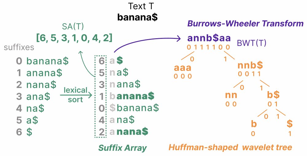
Figure 2: The FM-index data structure (§2.1) used in infini-gram mini, shown for a toy string with length $n=7$. The suffix array is sampled with a sampling rate $a=3$ and only elements corresponding to bolded suffixes are stored. The BWT can be derived from the SA, and is stored in compressed form as a Huffman-shaped wavelet tree.

图 2：infini-gram mini 所用 FM-index 数据结构（§2.1），玩具串长度 $n=7$。后缀数组采样率 $a=3$，仅存对应加粗后缀的元素。BWT 可由 SA 导出，并以 Huffman 形状小波树压缩存储。

Suffix array and sampling.

The suffix array $\mathit{SA}$ of a string $T$ of length $n$ is an array of integers representing the starting positions of all suffixes of $T$ in lexicographic order. Formally, $\mathit{SA}[i]=j$ if the suffix $T[j...n]$ ranks $i$th among all suffixes in lexicographical ordering. The suffix array enables quickly locating the positions where a pattern appears in the string. Canonically, storing the whole suffix array would take $O(n\log n)$ space, or $5n$ bytes for strings with length up to one trillion (Liu et al. 2024). To reduce storage overhead, FM-index samples $\mathit{SA}$ at regular intervals, storing only every $a$th entry where $a$ is a parameter. When querying the index, if we need to access an unsampled $\mathit{SA}$ entry, we can recover its value by referencing the BWT data structure, which is introduced below.

后缀数组与采样。

长度 $n$ 的串 $T$ 的后缀数组 $\mathit{SA}$ 是按字典序排列的全部后缀起始位置。形式化地，$\mathit{SA}[i]=j$ 表示后缀 $T[j...n]$ 在字典序中排第 $i$。后缀数组可快速定位模式出现位置。经典做法存完整 SA 需 $O(n\log n)$ 空间，对万亿级长度约 $5n$ 字节（Liu 等 2024）。为降开销，FM-index 按间隔采样，只存每隔 $a$ 个条目。查询若需未采样条目，可借助下文 BWT 结构恢复。

Burrows-Wheeler transform (BWT).

BWT (Burrows et al. 1994) rearranges the string $T$ (with termination symbol $) into a reversible permutation$L$that clusters repeated symbols. The BWT is defined as a string$L$where$L[i]=T[\mathit{SA}[i]-1]$if$SA[i]>0$, or$L[i]=$$otherwise. Intuitively,$L$ is the concatenation of the symbol preceding each suffix when the suffixes are sorted in the SA order (see Figure 2).

Burrows-Wheeler 变换（BWT）。

BWT（Burrows 等 1994）把带终止符 $的$T$重排为可逆置换$L$，使重复符号聚集。定义为：$L[i]=T[\mathit{SA}[i]-1]$（若$SA[i]>0$），否则$L[i]=$$。直观上，$L$ 是按 SA 序排列各后缀前一符号的拼接（见图 2）。

A key property of BWT is the Last-to-First (LF) mapping, which maps the $i$th occurrence of a symbol $c$ in $L$ to the $i$th occurrence of it in $T$. The LF mapping is defined as $\mathit{LF}(i)=C[c]+\text{rank}(c,i)$, where $C[c]$ is the number of symbols in $L$ lexicographically smaller than $c$, and $\text{rank}(c,i)$ counts the occurrences of $c$ in $L[0...i]$. This property allows us to traverse the string in reverse order, which is essential for finding patterns in and reconstructing (part of) the string $T$ from the index.

BWT 的关键性质是 Last-to-First（LF）映射：把 $L$ 中符号 $c$ 的第 $i$ 次出现映到 $T$ 中其第 $i$ 次出现。$\mathit{LF}(i)=C[c]+\text{rank}(c,i)$，其中 $C[c]$ 为 $L$ 中字典序小于 $c$ 的符号数，$\text{rank}(c,i)$ 计 $L[0...i]$ 中 $c$ 的出现次数。该性质支持反向遍历字符串，对在索引中找模式并重建（部分）$T$ 至关重要。

Huffman-shaped wavelet trees.

Given the BWT $L$ and the sampled SA, we can reconstruct the original string $T$ from these data structures so we don’t need to store $T$. However, $L$ still takes as much storage as $T$. To further compress $L$, a wavelet tree is used to represent $L$ by hierarchically partitioning the alphabet. In the wavelet tree, each leaf node represents a symbol in the alphabet, and each non-leaf node stores a bitvector marking whether the symbol at each position of $L$ belongs to the left or right subtree. A Huffman-shaped wavelet tree (Mäkinen and Navarro 2005) optimizes the hierarchy by grouping and coding symbols based on their frequencies in $L$. Storing it costs $(nH_{0}+2\sigma\log n)$ bits, where $\sigma$ is the alphabet size, and $H_{0}$ is the zeroth-order entropy of $L$ and $H_{0}\approx 0.26\log_{2}{\sigma}$ in our experiments with natural language text; this is smaller than storing $L$ directly, which is $n\log_{2}{\sigma}$ bits. Besides compression, the tree can efficiently support two operations crucial to LF mapping: $\text{rank}(c,\ell)$ counts the number of occurrences of a character $c$ in $L[0...\ell-1]$, and $\text{select}(c,m)$ finds the position of the $m$th occurrence of $c$ in $L$. Both operations have a time complexity of $O(H_{0})$.

Huffman 形状小波树。

有了 BWT $L$ 与采样 SA，可从这些结构重建 $T$，无需再存 $T$。但 $L$ 仍与 $T$ 同体积。为进一步压缩，用小波树按字母表层次划分表示 $L$：叶节点对应符号，非叶存位向量标示各位置属左或右子树。Huffman 形状小波树（Mäkinen and Navarro 2005）按 $L$ 中频率分组编码以优化层次。存储代价 $(nH_{0}+2\sigma\log n)$ 比特，$\sigma$ 为字母表大小，$H_{0}$ 为 $L$ 零阶熵；我们自然语言实验中 $H_{0}\approx 0.26\log_{2}{\sigma}$，小于直接存 $L$ 的 $n\log_{2}{\sigma}$ 比特。树还高效支持 LF 映射所需的 $\text{rank}(c,\ell)$ 与 $\text{select}(c,m)$，复杂度均为 $O(H_{0})$。

Inverse suffix array.

To allow reconstructing part of the original string $T$ from any given position, FM-index also stores a sampled version of the inverse suffix array $\mathit{ISA}$. $\mathit{ISA}$ is the inverse of the permutation specified in $\mathit{SA}$ and is defined as $\mathit{ISA}[j]=i$ if $\mathit{SA}[i]=j$. When reconstructing $T$ from a given position, $\mathit{ISA}$ is used to identify the corresponding rank in the suffix array to start reconstruction. In FM-index, we can use a different sampling rate for $\mathit{ISA}$, storing only every $b$th entry, where $b$ can be larger than $a$ as $\mathit{ISA}$ is used less.

逆后缀数组。

为从任意位置重建部分原串 $T$，FM-index 还存采样的逆后缀数组 $\mathit{ISA}$。$\mathit{ISA}$ 是 $\mathit{SA}$ 置换的逆：$\mathit{ISA}[j]=i$ 当 $\mathit{SA}[i]=j$。重建时用 $\mathit{ISA}$ 找到对应 SA 秩作为起点。采样率可用不同的 $b$，且可大于 $a$，因 $\mathit{ISA}$ 使用更少。

2.2 Querying the FM-index

2.2 查询 FM-index

There are three basic operations supported by FM-index: find, locate, and reconstruct. Counting a pattern can be done with a find operation, and retrieving segments containing the pattern from the original string can be done with a combination of all three operations. See App. §A for more details.

FM-index 支持三种基本操作：find、locate、reconstruct。计数模式可用 find；取回含模式的片段需三者组合。细节见附录 §A。

3 Infini-gram mini

We develop infini-gram mini as a scalable and efficient implementation of FM-index on natural language data. For indexing, infini-gram mini achieves 18$\times$ speedup and reduces RAM usage by 3.2$\times$ compared to the previous best existing implementation in SDSL. This paves way for indexing petabyte-level text corpora with reasonable time and compute. For querying, we extended the implementation in SDSL to work with indexes stored on disk, allowing us to query large indexes on machines with limited RAM.

我们开发 infini-gram mini，作为自然语言数据上可扩展、高效的 FM-index 实现。建索引相对 SDSL 先前最佳实现提速 18$\times$、RAM 降 3.2$\times$，为以合理时间与算力索引拍字节语料铺路。查询侧扩展 SDSL 以支持磁盘索引，便于在有限 RAM 机器上查询大索引。

In contrast to the original infini-gram which tokenizes the text, we construct the index directly on raw UTF-8 bytes, which saves tokenization time and allows more flexibility when querying. Tokenization is a technique to reduce index size, but since FM-index is already a compressed index, tokenization would not be helpful here.

相对对文本分词的原始 infini-gram，我们直接在原始 UTF-8 字节上建索引，省去分词时间且查询更灵活。分词本可缩小索引，但 FM-index 已是压缩索引，此处分词无益。

3.1 Index Construction

3.1 索引构建

Optimizing the indexing steps.

We use a parallelized implementation of each indexing step. For building SA and BWT, we adapt from the parallel implementation in Liu et al. 2024. For building the wavelet tree, we use the parallel implementation in Labeit et al. 2017. For sampling SA and creating a sampled version of ISA, we parallelized the implementation in SDSL. All these steps were single-threaded in SDSL, and by parallelizing them we achieve significant speedup.

优化建索引步骤。

各步骤均并行化。SA 与 BWT 改编自 Liu 等 2024 的并行实现；小波树用 Labeit 等 2017 的并行实现；采样 SA 与构建采样 ISA 则把 SDSL 实现并行化。这些步骤在 SDSL 中均为单线程，并行后显著加速。

We measured the time and peak RAM usage for indexing an 8.7 GB corpus (a single file from DCLM-baseline) using implementation of SDSL and infini-gram mini. Their implementation required 5,847 seconds and 74,807 MB of peak RAM, whereas infini-gram mini completed indexing in 324 seconds (18$\times$ speedup) and peak RAM of 23,742 MB (3.2$\times$ reduction).

我们在 8.7 GB 语料（DCLM-baseline 单文件）上对比 SDSL 与 infini-gram mini：前者 5,847 秒、峰值 RAM 74,807 MB；后者 324 秒（18$\times$）与 23,742 MB（降 3.2$\times$）。

Preprocessing.

FM-index is designed to work on a single string. To index a text corpora, which consists of a collection of documents, we encode all documents with UTF-8 and concatenate all these byte arrays with the \xff byte (not used by UTF-8) to mark document boundaries. We then construct FM-index for this big byte string. We work on UTF-8 bytes rather than characters to keep the alphabet size small ($\sigma=256$). Along with this text index, we also store a text offset file that records the starting position of each document, which is useful for retrieving whole document and metadata. Aside from the actual text, we also index the metadata of the documents to make the metadata searchable while storing it in a similar compressed form.

预处理。

FM-index 面向单串。语料由多文档组成时，用 UTF-8 编码并以 UTF-8 未用的 \xff 字节拼接标记边界，再对该大字节串建索引。用字节而非字符以保持字母表小（$\sigma=256$）。除 文本索引 外，还存 文本偏移 文件记录各文档起点，便于取整篇与元数据。元数据亦建索引，使其可检索并以类似压缩形式存储。

Partitioning.

For large corpora, we partition it into multiple shards and index each shard independently. Searching across multiple shards produces the same result as searching a single, larger index, and this allows us to build indexes with limited RAM per node as well as embarrassingly parallelize across multiple nodes.

分片。

大语料分成多 shard 独立建索引。跨 shard 检索结果与单一更大索引一致，便于单节点有限 RAM，也可跨节点 embarrassingly 并行。

Indexed corpora.

We have built the index for the following corpora: the Pile (1.3TB training set, 1.4GB validation set; Gao et al. 2020), DCLM-baseline (17TB; Li et al. 2024), and the Common Crawl between January and March 2025 (“CC-2025-05”, “CC-2025-08”, “CC-2025-13”; 28TB total; Common Crawl Foundation 2025).[^2]

已索引语料。

已建索引：Pile（训练 1.3TB、验证 1.4GB；Gao 等 2020）、DCLM-baseline（17TB；Li 等 2024），以及 2025 年 1–3 月 Common Crawl（“CC-2025-05”“CC-2025-08”“CC-2025-13”；合计 28TB；Common Crawl Foundation 2025）。[^2]

Dataset	Original Size	Indexing Time	Index Size	Num. Shards
	(TB)	(CPU node-days)	(TB)
Pile-validation	0.0001345	0.00057	0.000602 (0.45$\times$)	1
Pile-train	1.308	1.31	0.588 (0.45$\times$)	2
DCLM-baseline	16.666	12.6	7.523 (0.45$\times$)	25
CC-2025-05	9.079	11.8	3.972 (0.44$\times$)	15
CC-2025-08	8.163	10.6	3.574 (0.44$\times$)	15
CC-2025-13	10.393	13.6	4.563 (0.44$\times$)	17
Total	45.610	49.8	20.131 (0.44$\times$)	75

Table 1: Text corpora we indexed with infini-gram mini, along with indexing time and index size. The reported numbers only include actual document content and do not include metadata.

Dataset	Original Size	Indexing Time	Index Size	Num. Shards
	(TB)	(CPU node-days)	(TB)
Pile-validation	0.0001345	0.00057	0.000602 (0.45$\times$)	1
Pile-train	1.308	1.31	0.588 (0.45$\times$)	2
DCLM-baseline	16.666	12.6	7.523 (0.45$\times$)	25
CC-2025-05	9.079	11.8	3.972 (0.44$\times$)	15
CC-2025-08	8.163	10.6	3.574 (0.44$\times$)	15
CC-2025-13	10.393	13.6	4.563 (0.44$\times$)	17
Total	45.610	49.8	20.131 (0.44$\times$)	75

表 1：用 infini-gram mini 索引的文本语料、建索引时间与索引体积。数字仅含文档正文，不含元数据。

Indexing time.

We use CPU nodes with 128 vCPUs and 2TiB RAM to construct indexes, and under this constraint, each shard can be as large as 700GB which can be indexed in 12–19 hours. Table 1 reports the time for indexing the above corpora. Indexing time shows a slightly super-linear increase with respect to shard size, and we report detailed stepwise breakdown in App. §B. If we were to index the full Common Crawl dataset (about 1PB), we would split it into 1,500 shards, which can be indexed in 1,200 node-days.

建索引时间。

使用 128 vCPU、2TiB RAM 的 CPU 节点；该约束下每 shard 最大约 700GB，建索引 12–19 小时。表 1 报告上述语料时间。时间随 shard 大小略超线性增长，分步细节见附录 §B。若索引完整 Common Crawl（约 1PB），可分 1,500 shard，约 1,200 节点·天。

Index size.

We choose the sampling rate empirically to balance storage savings and query latency. In our implementation, we sample every $a=32$ entries of SA and every $b=64$ entries of ISA. This yields indexes with 0.44$\times$ the size of the corpora (Table 1). Conceptually, if we set $a$ and $b$ to be very big, then the SA and ISA would have negligible size, and the index can be as small as 0.26$\times$ the size of the corpus.

索引体积。

经验选择采样率以平衡存储与查询延迟。实现中 SA 每隔 $a=32$、ISA 每隔 $b=64$ 采样，得到约为语料 0.44$\times$ 的索引（表 1）。概念上若 $a$、$b$ 很大，SA/ISA 可忽略，索引可低至语料 0.26$\times$。

3.2 Querying with infini-gram mini

3.2 用 infini-gram mini 查询

Similar to other exact-match search engines, infini-gram mini supports two types of query: counting the number of occurrences of a string, and retrieving documents that contain a string. At query time, infini-gram mini keeps all index files on disk as memory-mapped files, thus requiring only minimal CPU and RAM.

与其他精确匹配引擎类似，支持两类查询：计数字符串出现次数，以及取回含该串的文档。查询时全部索引文件以内存映射驻留磁盘，仅需极少 CPU 与 RAM。

Querying in infini-gram mini is slower and more complex than in canonical suffix arrays due to the compressive nature of FM-index. The SA is subsampled, and the original text is shuffled and compressed, both requiring additional random disk reads to recover. The latency of queries is largely determined by the disk I/O performance.

因 FM-index 的压缩特性，查询比经典后缀数组更慢更复杂：SA 被子采样，原文被打乱压缩，都需额外随机磁盘读恢复。延迟很大程度上取决于磁盘 I/O。

Counting a string.

We use FM-index’s find operation to count the number of occurrences of a query string. We parallelize this operation across all $k$ shards, and report the sum of counts across all shards. The total number of random disk reads is $O(k|Q|H_{0})$, where $|Q|$ is the length of the query string. If the disk’s I/O throughput is high enough, the query latency can be as low as $O(|Q|H_{0})$.

计数字符串。

用 find 计数查询串出现。跨全部 $k$ 个 shard 并行，再求和。随机磁盘读次数 $O(k|Q|H_{0})$，$|Q|$ 为查询长度。若磁盘吞吐够高，延迟可低至 $O(|Q|H_{0})$。

Retrieving documents.

We first use the find operation to get the range in the SA that corresponds to the query string. Each element in this range indicates one appearance of the query string in the text corpus. If the index has multiple shards, we will have one range for each shard. For each element in this range, we can use the locate operation to find the position of the match in the original text $T$, then get the boundaries of the enclosing document with a binary search in the text offset file, and finally use the reconstruct operation to get the document text. The number of random disk reads for locate is $O(aH_{0})$, and for reconstruct is $O((b+d)H_{0})$ where $d$ is the document length. We parallelize reconstruct operation by dividing document text into up to $t=10$ chunks, or chunks of length 100 if $d<1000$. Retrieving a single document is parallelized across $t$ threads, and it can be further parallelized for retrieving multiple documents.

取回文档。

先 find 得到查询串对应的 SA 区间；区间内每个元素对应一次出现。多 shard 时每 shard 一个区间。对每个元素用 locate 找原串 $T$ 中位置，再在文本偏移文件二分得到包围文档边界，最后 reconstruct 得到文档文本。locate 随机读 $O(aH_{0})$，reconstruct 为 $O((b+d)H_{0})$，$d$ 为文档长度。我们将文档切成最多 $t=10$ 块（若 $d<1000$ 则每块长 100）并行 reconstruct；单文档内 $t$ 线程并行，多文档可进一步并行。

Query latency.

Infini-gram mini presents second-level latency on both types of query. We benchmark the query latency with the index files stored on Google GCP SSD disks with 80,000 IOPS and 1200 MB/s throughput. We measure the average latency over 100 queries for each query type and setting. For counting, short queries ($|Q|\leq 10$) can be handled within 0.4 seconds for all corpora we indexed, while longer queries ($|Q|=1000$) are handled in 8 seconds for CC-2025-05 and 25 seconds for DCLM-baseline. The difference in query latency is caused by the different number of shards in the corpora. For document retrieval, retrieving a snippet of $d=100$ bytes can be done within 2 seconds for all corpora, and retrieving $d=3000$ bytes takes up to 4.5 seconds. See App. §C for benchmarking details.

查询延迟。

两类查询均为秒级。索引存于 Google GCP SSD（80,000 IOPS、1200 MB/s），每类设置平均 100 次查询。计数：短查询（$|Q|\leq 10$）在全部已索引语料上 0.4 秒内；长查询（$|Q|=1000$）在 CC-2025-05 约 8 秒、DCLM-baseline 约 25 秒，差异来自分片数。文档取回：$d=100$ 字节片段 2 秒内，$d=3000$ 最多约 4.5 秒。细节见附录 §C。

3.3 Web Interface and API Endpoint

3.3 Web 界面与 API 端点

We host a web interface for easy access to counting and document retrieval with 45.6 TB corpora (App. §D). We also release an API endpoint that allows programmatically submitting requests.

我们托管 Web 界面，便于在 45.6 TB 语料上计数与取回文档（附录 §D），并发布可编程提交请求的 API 端点。

4 Analyzing and Monitoring Benchmark Contamination with infini-gram mini

4 用 infini-gram mini 分析与监测基准污染

In this section, we showcase how infini-gram mini can be used to analyze benchmark contamination at scale. Infini-gram mini allows us to search in the largest body of text ever in the open-source community with minimal storage overhead, enabling large-scale benchmark contamination analysis at low cost. Our work also supports analyzing new benchmarks uploaded later.

本节展示如何用它做大规模基准污染分析。系统能以极低存储开销检索开源社区迄今最大文本体量，低成本支撑大规模污染分析，也支持日后上传的新基准。

By identifying lexical overlap between 24 widely-used evaluation benchmarks and three major corpora, we find non-trivial contamination across 12 benchmarks (§4.2). We then retrieve documents accounting for contamination for further analysis (§4.3). Powered by infini-gram mini, we develop a monitoring system with a benchmark contamination bulletin, where we continuously monitor new crawls and report benchmarks’ contamination status over time (§4.4). We also invite the community to contribute by suggesting additional benchmarks or uploading new ones for analysis.

通过度量 24 个常用评测基准与三大语料的词汇重叠，我们发现 12 个基准存在不可忽视污染（§4.2）。再取回造成污染的文档细查（§4.3）。基于此构建监测系统与污染公告板，持续跟踪新爬取并报告污染随时间变化（§4.4），并邀请社区建议或上传新基准。

Infini-gram mini has further potential applications where exact-match search is needed, including (1) task-specific dataset construction, where creation of those datasets requires retrieving documents containing specific terms or phrases, and (2) data curation, where infini-gram mini can assist in identifying and removing duplicate, low-quality, or sensitive text and documents. We leave these directions for future exploration.

需要精确匹配检索时还有更多潜力：(1) 任务特定数据构建——按术语/短语取回文档；(2) 数据策展——辅助识别并移除重复、低质或敏感文本。这些方向留待未来。

4.1 Setup

4.1 设置

Contamination detection method.

We check contamination of test examples by measuring lexical overlap with the text corpus, following standard practice in the literature (Brown et al. 2020; Llama Team 2024). Given a text entry, we extract all 50-character substrings $S$ with a stride of one word, and determine entry contamination based on the proportion of substrings that appear at least once in the corpus:

污染检测方法。

按文献惯例（Brown 等 2020；Llama Team 2024），用与语料的词汇重叠检查测试例污染。给定条目，按词步长抽取全部 50 字符子串 $S$，按至少出现一次的子串比例判定：

$$\eta=\frac{\sum_{s\in S}\mathbb{I}\big[\texttt{count}(s)>0\big]}{|S|}.$$

We classify an entry into three contamination levels using the same thresholds with different namings as Touvron et al. 2023:

我们用与 Touvron 等 2023 相同阈值、不同命名，将条目分为三档污染水平：

• • Clean, if $\eta<20\%$

• • 干净，若 $\eta<20\%$

• • Suspicious, if $20\%\leq\eta<80\%$

• • 可疑，若 $20\%\leq\eta<80\%$

• • Dirty, if $\eta\geq 80\%$

• • 脏，若 $\eta\geq 80\%$

Benchmarks.

To comprehensively evaluate contamination, we analyze a broad range of benchmarks widely used to evaluate state-of-the-art LMs. We categorize benchmarks into five groups based on their primary focus: (1) knowledge and reasoning, i.e., understanding and reasoning over factual and conceptual knowledge; (2) math, i.e., mathematical reasoning ability; (3) code generation and modification abilities; (4) commonsense understanding, i.e., commonsense knowledge and reasoning abilities; and (5) reading comprehension of textual context. In total, we analyze 24 benchmarks; see App. §E for the full list and citations.

基准。

为全面评估，我们分析广泛用于前沿 LM 的基准，按主要关注点分为五组：(1) 知识与推理；(2) 数学；(3) 代码生成与修改；(4) 常识理解；(5) 阅读理解。共 24 个基准；完整列表与引用见附录 §E。

For benchmarks with question-answering format, we specifically check the question entries for contamination. Questions are usually longer and contain sufficient contextual information to uniquely identify the benchmark example, whereas answers can be short, such as a multiple choice option or a number. For language understanding tasks that involve reading a context or paragraph before answering, we check the context entries for contamination.

对问答格式基准，重点检查问题条目：问题通常更长且含足以唯一标识样例的上下文，而答案可能很短（选项或数字）。对需先读上下文再作答的语言理解任务，则检查上下文条目。

We evaluate on only the test set of benchmarks. For benchmarks with large test set, we downsample to 1,000 entries for efficiency. For benchmarks with multiple subtasks, we sample proportionally from each subtask to maintain representative distribution.

仅在测试集上评估。测试集过大时下采样至 1,000 条；多子任务时按比例抽样以保持代表性。

4.2 Results

4.2 结果

Table 2 reports the percentage of dirty entries in benchmarks against the Pile (knowledge cutoff in 2020), DCLM-baseline (knowledge cutoff in 2022), and CC-2025-05 (knowledge cutoff in January 2025). The detailed count of dirty and suspicious entries can be found in App. §F.

表 2 报告相对 Pile（知识截止 2020）、DCLM-baseline（2022）与 CC-2025-05（2025 年 1 月）的脏条目百分比。脏/可疑计数细节见附录 §F。

Many widely-used benchmarks are highly contaminated.

When checking against DCLM-baseline, MMLU has 27.70% dirty entries, MMLU-Pro has 16.20%, ARC-Challenge has 32.6%, and ARC-Easy has 32.3%. These benchmarks, especially MMLU, have been used to evaluate virtually every new LM in recent years. We believe that the observed contamination levels are a strong signal that many recently reported results may overestimate language model abilities on truly new, unseen evaluation items.

许多常用基准高度污染。

相对 DCLM-baseline，MMLU 脏率 27.70%，MMLU-Pro 16.20%，ARC-Challenge 32.6%，ARC-Easy 32.3%。尤其 MMLU 几乎被近年每个新 LM 用来评测。我们认为这些污染水平强烈提示：许多近期报告可能高估了模型在真正未见评测项上的能力。

Larger and newer corpora show greater contamination.

Compared with Pile-train, most benchmarks show a higher dirty rate on DCLM-baseline. For example, ARC-Challenge has 17$\times$ more and MMLU has 1.1$\times$ more dirty entries. However, CC-2025-05 has lower contamination rate than DCLM-baseline on most benchmarks, which is likely because DCLM-baseline corpus is larger and is a high-quality subset of crawls spanning a decade, while CC-2025-05 is an unfiltered single crawl.

更大更新的语料污染更重。

相对 Pile-train，多数基准在 DCLM-baseline 上脏率更高，例如 ARC-Challenge 多 17$\times$、MMLU 多 1.1$\times$。但 CC-2025-05 在多数基准上低于 DCLM-baseline，可能因 DCLM 更大且是跨十年爬取的高质量子集，而 CC-2025-05 是未过滤的单次爬取。

Contamination level varies by domain.

Benchmarks in historically-significant domains, such as commonsense understanding (e.g., ARC, OpenbookQA) and reading comprehension (e.g., SQuAD, CoQA), tend to show higher dirty rates on all corpora, while those in emerging domains like math (e.g., GSM8K, MATH-500) and code (e.g., HumanEval, LiveCodeBench) remain relatively clean at this writing.

污染水平因领域而异。

历史上重要领域如常识（ARC、OpenbookQA）与阅读理解（SQuAD、CoQA）在各语料上脏率往往更高；新兴领域如数学（GSM8K、MATH-500）与代码（HumanEval、LiveCodeBench）写作时仍相对干净。

New benchmarks are gradually getting contaminated in recent corpora.

Newer benchmarks are initially clean on earlier corpora. For example, AIME-2024 and GPQA are uncontaminated on Pile-train and DCLM-baseline, but show 10.00% and 0.89% dirty rate on the more recent CC-2025-05, respectively. GSM8K is very clean on Pile-train and DCLM-baseline, but has 5.5% dirty entries on CC-2025-05.

新基准在近期语料中逐渐被污染。

较新基准在早期语料上起初干净。例如 AIME-2024 与 GPQA 在 Pile-train 与 DCLM 上未污染，但在更新的 CC-2025-05 上脏率分别为 10.00% 与 0.89%。GSM8K 在前两者很干净，在 CC-2025-05 有 5.5% 脏条目。

	Test Size	Pile-train	DCLM-baseline	CC-2025-05	CC-2025-08
Knowledge and Reasoning
MMLU	1000	13.20	27.70	13.50	9.00
MMLU-Pro	1000	5.90	16.20	7.10	5.40
BigBenchHard	1000	0.00	0.10	1.40	1.40
AGIEval	1000	0.80	3.10	2.70	3.60
GPQA	448	0.00	0.00	0.89	2.01
HLE	881	0.00	0.00	0.00	0.00
Math
AIME-2024	30	0.00	0.00	10.00	3.33
GSM8K	1000	0.00	0.20	5.50	0.80
MATH-500	500	0.60	3.20	0.60	7.80
MGSM	250	0.00	0.00	5.60	1.60
Code
HumanEval	164	0.00	0.00	0.00	0.61
HumanEval+	164	0.00	0.00	0.00	0.61
LiveCodeBench	880	0.00	0.00	0.00	0.00
SWE-bench	500	0.00	0.00	0.20	0.20
MBPP	500	0.00	0.40	1.00	1.40
Commonsense Understanding
ARC-Challenge	1000	1.40	32.60	11.90	4.00
ARC-Easy	1000	1.50	32.30	5.40	9.50
CSQA	1000	0.10	1.00	0.10	0.10
HellaSwag	1000	0.00	0.00	0.00	0.00
OpenbookQA	500	10.80	15.60	14.60	30.20
Social IQa	1000	0.00	0.50	0.20	4.40
WinoGrande	1000	0.00	0.00	0.00	0.00
Reading Comprehension
CoQA	500	8.00	18.40	7.40	8.80
SQuAD	1000	2.80	40.10	2.70	33.00

Table 2: Dirty rates for benchmarks across the Pile, DCLM-baseline, CC-2025-05, and CC-2025-08. Full result is reported in Table 6. For benchmark entries with over 1000 entries, we report dirty rate on the downsampled subset. Cell background color indicates benchmark cleaniness, with green representing clean benchmarks and red representing increasing levels of contamination.

	Test Size	Pile-train	DCLM-baseline	CC-2025-05	CC-2025-08
Knowledge and Reasoning
MMLU	1000	13.20	27.70	13.50	9.00
MMLU-Pro	1000	5.90	16.20	7.10	5.40
BigBenchHard	1000	0.00	0.10	1.40	1.40
AGIEval	1000	0.80	3.10	2.70	3.60
GPQA	448	0.00	0.00	0.89	2.01
HLE	881	0.00	0.00	0.00	0.00
Math
AIME-2024	30	0.00	0.00	10.00	3.33
GSM8K	1000	0.00	0.20	5.50	0.80
MATH-500	500	0.60	3.20	0.60	7.80
MGSM	250	0.00	0.00	5.60	1.60
Code
HumanEval	164	0.00	0.00	0.00	0.61
HumanEval+	164	0.00	0.00	0.00	0.61
LiveCodeBench	880	0.00	0.00	0.00	0.00
SWE-bench	500	0.00	0.00	0.20	0.20
MBPP	500	0.00	0.40	1.00	1.40
Commonsense Understanding
ARC-Challenge	1000	1.40	32.60	11.90	4.00
ARC-Easy	1000	1.50	32.30	5.40	9.50
CSQA	1000	0.10	1.00	0.10	0.10
HellaSwag	1000	0.00	0.00	0.00	0.00
OpenbookQA	500	10.80	15.60	14.60	30.20
Social IQa	1000	0.00	0.50	0.20	4.40
WinoGrande	1000	0.00	0.00	0.00	0.00
Reading Comprehension
CoQA	500	8.00	18.40	7.40	8.80
SQuAD	1000	2.80	40.10	2.70	33.00

表 2：各基准在 Pile、DCLM-baseline、CC-2025-05 与 CC-2025-08 上的脏率。完整结果见表 6。超过 1000 条的测试集报告下采样子集脏率。单元格底色表示干净程度：绿为干净，红表示污染加重。

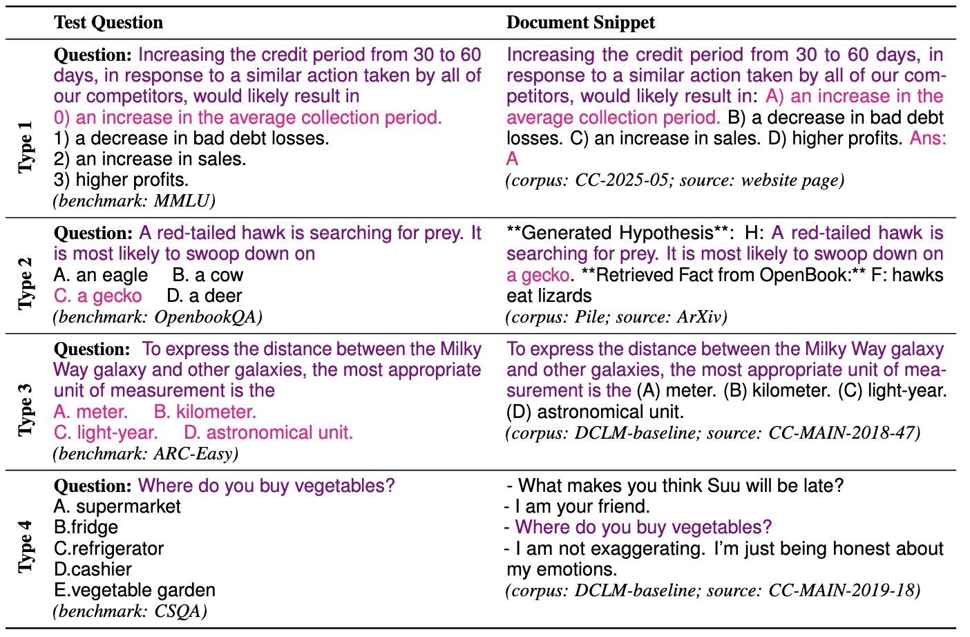
Figure 3: Examples of four contamination types. Violet text is the text overlap between benchmark entry and corpus. Magenta text is the mapping of answers.

图 3：四类污染示例。紫色为基准条目与语料重叠文本。品红为答案映射。

4.3 Analysis

4.3 分析

With infini-gram mini, we can retrieve documents from the corpus that contain contaminated examples for further analysis. We use LLM-as-a-judge to categorize all dirty instances into following scenarios (see App. §H for more details), with examples shown in Table 3:

借助系统可取回含污染样例的文档细查。我们用 LLM-as-a-judge 将全部脏实例归入下列情形（细节见附录 §H），示例见表 3：

• • Type 1: Question and answer appear as-is in corpus. The question and correct answer appear in the corpus in the exact format as in benchmark entry. The model may memorize entirely from these data instead of performing capabilities examined in benchmarks. This accounts for 72.5% of all dirty entries in Pile-train, 82.6% on DCLM-baseline, and 58% on CC-2025-05.

• • 类型 1：问题与答案原样出现在语料。 问题与正确答案以基准条目完全相同格式出现。模型可能整段记忆而非展现基准所考能力。占 Pile-train 脏条目 72.5%、DCLM 82.6%、CC-2025-05 58%。

• • Type 2: Question appeared, answer in natural language. The answer is expressed in natural language rather than the exact benchmark format, and model may directly infer the correct answer from it. This accounts for 4.5% of all dirty entries in Pile-train, 2.1% on DCLM-baseline, and 6.2% on CC-2025-05.

• • 类型 2：问题出现，答案以自然语言出现。 答案非基准精确格式，但模型可直接据此推出正确答案。占 Pile-train 4.5%、DCLM 2.1%、CC-2025-05 6.2%。

• • Type 3: Question appeared, no corresponding answer. The question (and maybe the multiple-choice options) appeared in the corpus, but correct answer is missing. This accounts for 18.1% of all dirty entries in Pile-train, 10.9% on DCLM-baseline, and 30.2% on CC-2025-05.

• • 类型 3：问题出现，无对应答案。 问题（及可能的选项）在语料中，但缺正确答案。占 Pile-train 18.1%、DCLM 10.9%、CC-2025-05 30.2%。

• • Type 4: False positives. There are documents that superficially match the question but are unrelated to the benchmark example. This happens on entries with a very short question. This accounts for 3.1% of all dirty entries in Pile-train, 1% on DCLM-baseline, and 3% on CC-2025-05.

• • 类型 4：假阳性。 文档表面匹配问题但与基准样例无关，常见于极短问题。占 Pile-train 3.1%、DCLM 1%、CC-2025-05 3%。

We shows 7 contamination examples in App. §G and its source of contamination. We found that contamination is caused by (1) the benchmark is sourced from the Internet (e.g., AIME-2024, Figure 6; SWE-bench, Figure 8), (2) there are other benchmarks or online quizzes that are sourced from the benchmark (e.g, GSM8K, Figure 10), (3) blogs and papers cite a benchmark entry as example (e.g, GPQA, Figure 9; BigBenchHard, Figure 11; OpenbookQA, Figure 12), and (4) benchmark entry coincide with online source (e.g., MMLU, Figure 7).

附录 §G 给出 7 个污染示例及其来源。污染原因包括：(1) 基准本身来自互联网（如 AIME-2024，图 6；SWE-bench，图 8）；(2) 其他基准或在线测验转引自该基准（如 GSM8K，图 10）；(3) 博客与论文引用某条目作例子（如 GPQA，图 9；BigBenchHard，图 11；OpenbookQA，图 12）；(4) 条目与网络来源巧合重合（如 MMLU，图 7）。

Contamination could cause LLM to overperform on evaluation benchmarks by enabling models to retrieve memorized answers from training data rather than performing task-specific reasoning. Our finding shows that a large majority of dirty entries contain exact matches of both question and answer, though even subtler forms of contamination such as question-only matches and paraphrased answers could inflate benchmark scores. As training corpora grow, the risk of benchmark contamination and the potential for rote memorization increase, making it more important to decontaminate training corpora and construct contamination-free benchmarks to avoid overestimating model capabilities.

污染可能使 LLM 在评测上虚高：从训练数据检索记忆答案而非做任务推理。我们发现多数脏条目同时精确匹配问题与答案；即便仅匹配问题或释义答案，也可能抬高分数。训练语料扩大后，污染与死记风险上升，更需对训练语料去污染并构建无污染基准，以免高估能力。

4.4 Benchmark Contamination Bulletin

4.4 基准污染公告板

Using infini-gram mini, we implement a benchmark contamination monitoring system that tracks benchmark contamination. In the future, we will keep indexing the latest crawl in Common Crawl and update contamination results to track benchmark contamination as corpora evolve. The system also allows anyone to add or upload new benchmarks to be monitored, fostering collaboration in benchmark monitoring. See App. §I for system interface.

我们实现持续跟踪污染的监测系统。未来将不断索引最新 Common Crawl 并更新结果。系统亦允许任何人添加或上传待监测基准，促进协作。界面见附录 §I。

5 Related Work

5 相关工作

Exact-match search in large text corpora.

Prior work has used different techniques to enable exact-match full-text search in large text corpora, including suffix arrays, suffix automata, and proprietary search engines. Below we survey the largest-scale implementation of each technique known to us. Merrill et al. 2024 applies suffix automaton on 1.3TB of text. Liu et al. 2024 applies suffix array on 12TB of text. Elazar et al. 2024 uses the proprietary ElasticSearch to index and analyze 35TB of text. All these methods have significant storage multiplier wrt the size of text indexed, ranging from ElasticSearch’s 2$\times$ to suffix automata’s 29$\times$. In contrast, our FM-index-based index has a storage multiplier as small as 0.26$\times$, allowing us to index the largest body of text ever in the open-source community.

大规模文本语料中的精确匹配检索。

先前工作用后缀数组、后缀自动机与专有搜索引擎等技术。据我们所知最大规模实现：Merrill 等 2024 在 1.3TB 上用后缀自动机；Liu 等 2024 在 12TB 上用后缀数组；Elazar 等 2024 用 ElasticSearch 分析 35TB。这些方法相对语料体积倍率从约 2$\times$ 到 29$\times$。我们基于 FM-index 的倍率可低至 0.26$\times$，从而索引开源社区迄今最大文本体量。

Benchmark contamination.

Benchmark contamination appeared as a critical concern in LLM evaluations in recent studies. Prior works has quantified benchmark contamination on open-sourced models using various matching strategies, including n-gram or token overlap (Soldaini et al. 2024; Llama Team 2024; Soldaini et al. 2024; OLMo et al. 2025), longest substring match (Singh et al. 2024), skipgram match (Touvron et al. 2023), and full-text exact match (Elazar et al. 2024). However, indexing large-scale pretraining corpora and performing exhaustive searches is computationally expensive, and prior studies on open corpora are limited in their scale (up to RedPajama-1T and Dolma, 12TB). To the best of our knowledge, our work conducts contamination analysis on the largest open corpora to date.

基准污染。

近期 LLM 评测中污染成关键关切。先前工作用 n-gram/词元重叠、最长子串、skipgram、全文精确匹配等量化开源模型污染。但索引大规模预训练语料并穷尽检索成本高，开源语料研究规模有限（最大约 RedPajama-1T 与 Dolma，12TB）。据我们所知，本文在迄今最大开源语料上做污染分析。

6 Conclusion

6 结论

We introduce infini-gram mini, an efficient system for indexing text with 0.44$\times$ their original size, enabling efficient counting and searching in massive text corpus, and we show its scalability to a petabyte-scale corpus. We showcase infini-gram mini’s application on benchmark contamination analysis at scale.

我们提出 infini-gram mini：以约 0.44$\times$ 原体积索引文本、在海量语料上高效计数与检索，并展示向拍字节语料扩展的可行性；同时展示其在大规模基准污染分析上的应用。

Limitations

局限

Although infini-gram mini shows significant improvements on text compression rate, document retrieval latency remains higher than a canonical suffix array. For example, reconstructing a 3000-character document takes 1.8 seconds on Pile and 4.5 seconds on DCLM-baseline, compared to millisecond-level retrieval in system like Infini-gram (Liu et al. 2024). This is a trade-off with infini-gram mini’s compression rate: infini-gram mini does not store the original text in a contiguous block. To retrieve a document, we need to reconstruct it character-by-character, leading to a large number of reads in random addresses. These process takes long time since the entire index is kept on disk at inference time. The high latency can potentially be reduced using techniques like disk page prefetching.

尽管压缩率显著提升，文档取回延迟仍高于经典后缀数组。例如重建 3000 字符文档在 Pile 约 1.8 秒、DCLM 约 4.5 秒，而 Infini-gram（Liu 等 2024）为毫秒级。这是压缩率的代价：不把原文连续存放，需逐字符重建，大量随机地址读；推理时整个索引在盘上，耗时长。可用磁盘页预取等技术缓解。

Identifying co-occurrences of multiple patterns is inefficient with the FM-index, since mapping every match from the suffix array range back to its position in original text takes very long time thus making this operation impractical. In contrast, the original infini-gram supports this operation efficiently.

用 FM-index 识别多模式共现低效：把后缀数组区间内每次匹配映回原文位置耗时过长，操作不现实。原始 infini-gram 对此更高效。

Infini-gram mini only supports exact-match searches. As a result, our benchmark contamination analysis is limited to case-sensitive exact matching, which may fail to detect contamination of instances with minor textual discrepancies.

仅支持精确匹配，故污染分析限于区分大小写的精确匹配，可能漏检仅有细微文本差异的污染。

As the text corpora may contain biased or toxic content, document retrieval output may contain content that can be perceived as ethically problematic, and may contain sensitive information. The output of infini-gram mini does not reflect authors’ views.

语料可能含偏见或有害内容，取回结果或被视为伦理问题，也可能含敏感信息。系统输出不代表作者观点。

Acknowledgments

致谢

We thank Christina Boucher (University of Florida) for telling us about the FM-index data structure. We would like to thank members of H2lab and AllenNLP for sharing their valuable feedback on this project.

感谢 Christina Boucher（University of Florida）向我们介绍 FM-index。感谢 H2lab 与 AllenNLP 成员对本项目的宝贵反馈。

References

参考文献

Austin et al. (2021) Jacob Austin, Augustus Odena, Maxwell Nye, Maarten Bosma, Henryk Michalewski, David Dohan, Ellen Jiang, Carrie Cai, Michael Terry, Quoc Le, and 1 others. 2021. Program synthesis with large language models. arXiv preprint arXiv:2108.07732 .

Brown et al. (2020) Tom B. Brown, Benjamin Mann, Nick Ryder, Melanie Subbiah, Jared Kaplan, Prafulla Dhariwal, Arvind Neelakantan, Pranav Shyam, Girish Sastry, Amanda Askell, Sandhini Agarwal, Ariel Herbert-Voss, Gretchen Krueger, Tom Henighan, Rewon Child, Aditya Ramesh, Daniel M. Ziegler, Jeffrey Wu, Clemens Winter, and 12 others. 2020. Language models are few-shot learners . Preprint , arXiv:2005.14165.

Burrows et al. (1994) Michael Burrows, D J Wheeler D I G I T A L, Robert W. Taylor, David J. Wheeler, and David Wheeler. 1994. A block-sorting lossless data compression algorithm .

Chen et al. (2021) Mark Chen, Jerry Tworek, Heewoo Jun, Qiming Yuan, Henrique Ponde de Oliveira Pinto, Jared Kaplan, Harri Edwards, Yuri Burda, Nicholas Joseph, Greg Brockman, Alex Ray, Raul Puri, Gretchen Krueger, Michael Petrov, Heidy Khlaaf, Girish Sastry, Pamela Mishkin, Brooke Chan, Scott Gray, and 39 others. 2021. Evaluating large language models trained on code . Preprint , arXiv:2107.03374.

Clark et al. (2018) Peter Clark, Isaac Cowhey, Oren Etzioni, Tushar Khot, Ashish Sabharwal, Carissa Schoenick, and Oyvind Tafjord. 2018. Think you have solved question answering? try arc, the ai2 reasoning challenge. arXiv:1803.05457v1 .

Cobbe et al. (2021) Karl Cobbe, Vineet Kosaraju, Mohammad Bavarian, Mark Chen, Heewoo Jun, Lukasz Kaiser, Matthias Plappert, Jerry Tworek, Jacob Hilton, Reiichiro Nakano, Christopher Hesse, and John Schulman. 2021. Training verifiers to solve math word problems. arXiv preprint arXiv:2110.14168 .

Common Crawl Foundation (2025) Common Crawl Foundation. 2025. Common crawl .

Elazar et al. (2024) Yanai Elazar, Akshita Bhagia, Ian Magnusson, Abhilasha Ravichander, Dustin Schwenk, Alane Suhr, Pete Walsh, Dirk Groeneveld, Luca Soldaini, Sameer Singh, Hanna Hajishirzi, Noah A. Smith, and Jesse Dodge. 2024. What’s in my big data? Preprint , arXiv:2310.20707.

Ferragina and Manzini (2000) P. Ferragina and G. Manzini. 2000. Opportunistic data structures with applications . In Proceedings 41st Annual Symposium on Foundations of Computer Science , pages 390–398.

Gao et al. (2020) Leo Gao, Stella Biderman, Sid Black, Laurence Golding, Travis Hoppe, Charles Foster, Jason Phang, Horace He, Anish Thite, Noa Nabeshima, Shawn Presser, and Connor Leahy. 2020. The Pile: An 800gb dataset of diverse text for language modeling. arXiv preprint arXiv:2101.00027 .

Gog et al. (2014) Simon Gog, Timo Beller, Alistair Moffat, and Matthias Petri. 2014. From theory to practice: Plug and play with succinct data structures. In 13th International Symposium on Experimental Algorithms, (SEA 2014) , pages 326–337.

Han and Tsvetkov (2022) Xiaochuang Han and Yulia Tsvetkov. 2022. Orca: Interpreting prompted language models via locating supporting data evidence in the ocean of pretraining data . ArXiv , abs/2205.12600.

Hendrycks et al. (2021) Dan Hendrycks, Collin Burns, Steven Basart, Andy Zou, Mantas Mazeika, Dawn Song, and Jacob Steinhardt. 2021. Measuring massive multitask language understanding . Preprint , arXiv:2009.03300.

Jain et al. (2024) Naman Jain, King Han, Alex Gu, Wen-Ding Li, Fanjia Yan, Tianjun Zhang, Sida Wang, Armando Solar-Lezama, Koushik Sen, and Ion Stoica. 2024. Livecodebench: Holistic and contamination free evaluation of large language models for code . Preprint , arXiv:2403.07974.

Jimenez et al. (2024) Carlos E. Jimenez, John Yang, Alexander Wettig, Shunyu Yao, Kexin Pei, Ofir Press, and Karthik Narasimhan. 2024. Swe-bench: Can language models resolve real-world github issues? Preprint , arXiv:2310.06770.

Labeit et al. (2017) Julian Labeit, Julian Shun, and Guy E. Blelloch. 2017. Parallel lightweight wavelet tree, suffix array and fm-index construction . Journal of Discrete Algorithms , 43:2–17.

Lee et al. (2022) Katherine Lee, Daphne Ippolito, Andrew Nystrom, Chiyuan Zhang, Douglas Eck, Chris Callison-Burch, and Nicholas Carlini. 2022. Deduplicating training data makes language models better . In Proceedings of the 60th Annual Meeting of the Association for Computational Linguistics (Volume 1: Long Papers) , pages 8424–8445, Dublin, Ireland. Association for Computational Linguistics.

Li (2014) Heng Li. 2014. Fast construction of fm-index for long sequence reads . Bioinformatics , 30(22):3274–3275.

Li et al. (2024) Jeffrey Li, Alex Fang, Georgios Smyrnis, Maor Ivgi, Matt Jordan, Samir Gadre, Hritik Bansal, Etash Guha, Sedrick Keh, Kushal Arora, Saurabh Garg, Rui Xin, Niklas Muennighoff, Reinhard Heckel, Jean Mercat, Mayee Chen, Suchin Gururangan, Mitchell Wortsman, Alon Albalak, and 40 others. 2024. Datacomp-lm: In search of the next generation of training sets for language models . Preprint , arXiv:2406.11794.

Lightman et al. (2023) Hunter Lightman, Vineet Kosaraju, Yura Burda, Harri Edwards, Bowen Baker, Teddy Lee, Jan Leike, John Schulman, Ilya Sutskever, and Karl Cobbe. 2023. Let’s verify step by step . Preprint , arXiv:2305.20050.

Liu et al. (2025) Jiacheng Liu, Taylor Blanton, Yanai Elazar, Sewon Min, YenSung Chen, Arnavi Chheda-Kothary, Huy Tran, Byron Bischoff, Eric Stuart Marsh, Michael Schmitz, Cassidy Trier, Aaron Sarnat, Jenna James, Jon Borchardt, Bailey Kuehl, Evie Cheng, Karen Farley, Sruthi Sreeram, Taira Anderson, and 12 others. 2025. Olmotrace: Tracing language model outputs back to trillions of training tokens .

Liu et al. (2024) Jiacheng Liu, Sewon Min, Luke Zettlemoyer, Yejin Choi, and Hannaneh Hajishirzi. 2024. Infini-gram: Scaling unbounded n-gram language models to a trillion tokens. arXiv preprint arXiv:2401.17377 .

Liu et al. (2023) Jiawei Liu, Chunqiu Steven Xia, Yuyao Wang, and Lingming Zhang. 2023. Is your code generated by chatGPT really correct? rigorous evaluation of large language models for code generation . In Thirty-seventh Conference on Neural Information Processing Systems .

Llama Team (2024) AI @ Meta Llama Team. 2024. The llama 3 herd of models . Preprint , arXiv:2407.21783.

Lu et al. (2024) Ximing Lu, Melanie Sclar, Skyler Hallinan, Niloofar Mireshghallah, Jiacheng Liu, Seungju Han, Allyson Ettinger, Liwei Jiang, Khyathi Chandu, Nouha Dziri, and Yejin Choi. 2024. Ai as humanity’s salieri: Quantifying linguistic creativity of language models via systematic attribution of machine text against web text . ArXiv , abs/2410.04265.

Mäkinen and Navarro (2005) Veli Mäkinen and Gonzalo Navarro. 2005. Succinct suffix arrays based on run-length encoding. In Combinatorial Pattern Matching , pages 45–56, Berlin, Heidelberg. Springer Berlin Heidelberg.

Merrill et al. (2024) William Merrill, Noah A. Smith, and Yanai Elazar. 2024. Evaluating n-gram novelty of language models using rusty-dawg . ArXiv , abs/2406.13069.

Mihaylov et al. (2018) Todor Mihaylov, Peter Clark, Tushar Khot, and Ashish Sabharwal. 2018. Can a suit of armor conduct electricity? a new dataset for open book question answering. In EMNLP .

of Problem Solving (2024) Art of Problem Solving. 2024. Aime problems and solutions .

OLMo et al. (2025) Team OLMo, Pete Walsh, Luca Soldaini, Dirk Groeneveld, Kyle Lo, Shane Arora, Akshita Bhagia, Yuling Gu, Shengyi Huang, Matt Jordan, Nathan Lambert, Dustin Schwenk, Oyvind Tafjord, Taira Anderson, David Atkinson, Faeze Brahman, Christopher Clark, Pradeep Dasigi, Nouha Dziri, and 21 others. 2025. 2 olmo 2 furious . Preprint , arXiv:2501.00656.

Phan et al. (2025) Long Phan, Alice Gatti, Ziwen Han, Nathaniel Li, Josephina Hu, Hugh Zhang, Chen Bo Calvin Zhang, Mohamed Shaaban, John Ling, and Sean Shi et al. 2025. Humanity’s last exam . Preprint , arXiv:2501.14249.

Rajpurkar et al. (2016) Pranav Rajpurkar, Jian Zhang, Konstantin Lopyrev, and Percy Liang. 2016. SQuAD: 100,000+ questions for machine comprehension of text . In Proceedings of the 2016 Conference on Empirical Methods in Natural Language Processing , pages 2383–2392, Austin, Texas. Association for Computational Linguistics.

Reddy et al. (2019) Siva Reddy, Danqi Chen, and Christopher D. Manning. 2019. CoQA: A conversational question answering challenge . Transactions of the Association for Computational Linguistics , 7:249–266.

Rein et al. (2023) David Rein, Betty Li Hou, Asa Cooper Stickland, Jackson Petty, Richard Yuanzhe Pang, Julien Dirani, Julian Michael, and Samuel R. Bowman. 2023. Gpqa: A graduate-level google-proof q&a benchmark . Preprint , arXiv:2311.12022.

Sakaguchi et al. (2019) Keisuke Sakaguchi, Ronan Le Bras, Chandra Bhagavatula, and Yejin Choi. 2019. Winogrande: An adversarial winograd schema challenge at scale . Preprint , arXiv:1907.10641.

Sap et al. (2019) Maarten Sap, Hannah Rashkin, Derek Chen, Ronan LeBras, and Yejin Choi. 2019. Socialiqa: Commonsense reasoning about social interactions . Preprint , arXiv:1904.09728.

Shi et al. (2022) Freda Shi, Mirac Suzgun, Markus Freitag, Xuezhi Wang, Suraj Srivats, Soroush Vosoughi, Hyung Won Chung, Yi Tay, Sebastian Ruder, Denny Zhou, Dipanjan Das, and Jason Wei. 2022. Language models are multilingual chain-of-thought reasoners . Preprint , arXiv:2210.03057.

Simpson and Durbin (2010) Jared T. Simpson and Richard Durbin. 2010. Efficient construction of an assembly string graph using the fm-index . Bioinformatics , 26(12):i367–i373.

Singh et al. (2024) Aaditya K. Singh, Muhammed Yusuf Kocyigit, Andrew Poulton, David Esiobu, Maria Lomeli, Gergely Szilvasy, and Dieuwke Hupkes. 2024. Evaluation data contamination in llms: how do we measure it and (when) does it matter? Preprint , arXiv:2411.03923.

Soldaini et al. (2024) Luca Soldaini, Rodney Kinney, Akshita Bhagia, Dustin Schwenk, David Atkinson, Russell Authur, Ben Bogin, Khyathi Chandu, Jennifer Dumas, Yanai Elazar, Valentin Hofmann, Ananya Jha, Sachin Kumar, Li Lucy, Xinxi Lyu, Nathan Lambert, Ian Magnusson, Jacob Morrison, Niklas Muennighoff, and 17 others. 2024. Dolma: an open corpus of three trillion tokens for language model pretraining research . In Proceedings of the 62nd Annual Meeting of the Association for Computational Linguistics (Volume 1: Long Papers) , pages 15725–15788, Bangkok, Thailand. Association for Computational Linguistics.

Suzgun et al. (2022) Mirac Suzgun, Nathan Scales, Nathanael Schärli, Sebastian Gehrmann, Yi Tay, Hyung Won Chung, Aakanksha Chowdhery, Quoc V Le, Ed H Chi, Denny Zhou, , and Jason Wei. 2022. Challenging big-bench tasks and whether chain-of-thought can solve them. arXiv preprint arXiv:2210.09261 .

Talmor et al. (2019) Alon Talmor, Jonathan Herzig, Nicholas Lourie, and Jonathan Berant. 2019. CommonsenseQA: A question answering challenge targeting commonsense knowledge . In Proceedings of the 2019 Conference of the North American Chapter of the Association for Computational Linguistics: Human Language Technologies, Volume 1 (Long and Short Papers) , pages 4149–4158, Minneapolis, Minnesota. Association for Computational Linguistics.

Touvron et al. (2023) Hugo Touvron, Louis Martin, Kevin R. Stone, Peter Albert, Amjad Almahairi, Yasmine Babaei, Nikolay Bashlykov, Soumya Batra, Prajjwal Bhargava, Shruti Bhosale, Daniel M. Bikel, Lukas Blecher, Cristian Cantón Ferrer, Moya Chen, Guillem Cucurull, David Esiobu, Jude Fernandes, Jeremy Fu, Wenyin Fu, and 49 others. 2023. Llama 2: Open foundation and fine-tuned chat models . ArXiv , abs/2307.09288.

Wang et al. (2018) Yuanrong Wang, Xueqi Li, Dawei Zang, Guangming Tan, and Ninghui Sun. 2018. Accelerating fm-index search for genomic data processing . In Proceedings of the 47th International Conference on Parallel Processing , ICPP ’18, New York, NY, USA. Association for Computing Machinery.

Wang et al. (2024) Yubo Wang, Xueguang Ma, Ge Zhang, Yuansheng Ni, Abhranil Chandra, Shiguang Guo, Weiming Ren, Aaran Arulraj, Xuan He, Ziyan Jiang, Tianle Li, Max Ku, Kai Wang, Alex Zhuang, Rongqi Fan, Xiang Yue, and Wenhu Chen. 2024. Mmlu-pro: A more robust and challenging multi-task language understanding benchmark . Preprint , arXiv:2406.01574.

Zellers et al. (2019) Rowan Zellers, Ari Holtzman, Yonatan Bisk, Ali Farhadi, and Yejin Choi. 2019. Hellaswag: Can a machine really finish your sentence? In Proceedings of the 57th Annual Meeting of the Association for Computational Linguistics .

Zhong et al. (2023) Wanjun Zhong, Ruixiang Cui, Yiduo Guo, Yaobo Liang, Shuai Lu, Yanlin Wang, Amin Saied, Weizhu Chen, and Nan Duan. 2023. Agieval: A human-centric benchmark for evaluating foundation models . Preprint , arXiv:2304.06364.

Appendix A Querying the FM-Index

附录 A 查询 FM-Index

This section introduces in details three operations supported by FM-index: find, locate, and reconstruct.

本节详细介绍 FM-index 支持的三种操作：find、locate 与 reconstruct。

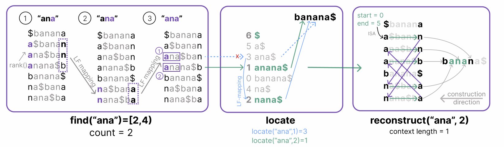
Figure 4: Illustration of operations on FM-index (§2.2, App. §A). Left: find operation computes the SA range corresponding to all occurrences of the pattern. Middle: locate operation computes the position of pattern occurrence in the original string for each position in the SA range. Right: reconstruct operation gets a substring of the original string enclosing the second pattern occurrence with a context length of 1. The occurrence ranking is based on its order in SA.

图 4：FM-index 操作示意（§2.2，附录 §A）。左： find 计算模式全部出现对应的 SA 区间。中： locate 把 SA 区间内每位映到原串中的模式出现位置。右： reconstruct 取包围第二次模式出现、上下文长度为 1 的原串子串。出现次序按其在 SA 中的顺序。

Find.

Each occurrence of a pattern string $Q$ in the haystack string $T$ corresponds to an element in the SA, and all these occurrences live in a consecutive range in the SA. The find operation computes this range with backward search: starting with the full range, it iterates through the symbols in $Q$ in reverse order, with each iteration narrowing the range using the character table $C$ and the rank operation of the BWT’s wavelet tree. The length of the final range is the count of $Q$ in $T$. Figure 4 (left) illustrates finding pattern “ana” in string “banana”. The time complexity of find is $O(|Q|H_{0})$, where $|Q|$ is the length of the pattern.

Find。

模式串 $Q$ 在草堆串 $T$ 中的每次出现对应 SA 中一个元素，且这些出现落在 SA 的连续区间。find 用反向搜索计算该区间：从全区间出发，按逆序遍历 $Q$ 中符号，每步用字符表 $C$ 与 BWT 小波树的 rank 收窄区间。最终区间长度即 $Q$ 在 $T$ 中的计数。图 4（左）示意在 “banana” 中找 “ana”。时间复杂度 $O(|Q|H_{0})$。

Locate.

The locate operation maps any position in the SA to its corresponding position in $T$. Since the SA is sampled at interval $a$, for an unsampled position $i$, the algorithm applies LF mapping at most $a$ times to locate the nearest sampled SA entry. Figure 4 (middle) illustrates locating the two occurrences of “ana” in “banana”. The time complexity of locating each position is $O(t_{\mathit{SA}})$, where $t_{\mathit{SA}}$ is the complexity of accessing an SA entry, which is $O(1)$ for sampled entries and $O(aH_{0})$ for unsampled entries.

Locate。

locate 把 SA 中任意位置映到 $T$ 中对应位置。因 SA 按间隔 $a$ 采样，对未采样位置 $i$，算法最多应用 $a$ 次 LF 映射找到最近采样 SA 条目。图 4（中）示意定位 “banana” 中两次 “ana”。每位定位复杂度 $O(t_{\mathit{SA}})$：采样条目 $O(1)$，未采样 $O(aH_{0})$。

Reconstruct.

After getting the position of a pattern occurrence in $T$, we can reconstruct a substring of $T$ enclosing that occurrence with some additional context. Starting at the end position of the desired substring, we apply the LF mapping to traverse through the BWT and use ISA to recover the symbol, and reconstruct symbols in reverse order until reaching the start position of the desired substring. Figure 4 (right) shows reconstructing the second occurrence of “ana” with context length of 1. The time complexity of reconstruct is $O(dH_{0}+t_{\mathit{ISA}})$, where $d$ is the length to reconstruct, and $t_{\mathit{ISA}}$ is the complexity of accessing an ISA entry, which is $O(1)$ for sampled entries and $O(bH_{0})$ for unsampled entries.

Reconstruct。

得到模式在 $T$ 中的位置后，可 reconstruct 包围该出现并带额外上下文的子串。从目标子串末端出发，用 LF 映射遍历 BWT 并用 ISA 恢复符号，逆序重建直至起点。图 4（右）示意重建第二次 “ana” 且上下文长度为 1。复杂度 $O(dH_{0}+t_{\mathit{ISA}})$，$d$ 为重建长度；采样 ISA 条目 $O(1)$，未采样 $O(bH_{0})$。

Appendix B Indexing Time

附录 B 建索引时间

Table 3presents indexing time for each shard of text corpora with stepwise breakdown. Suffix array construction scales super-linearly depending on the level of duplication (Lee et al. 2022). Constructing alphabet, wavelet tree, and sampling are linear operations. Indexing time also varies across similar-size shards originated from different text corpora, showing the time also depend on text corpora properties. For example, over 60% duplicate documents in the Pile (Elazar et al. 2024) causes SA construction to take significantly longer compared to DCLM-baseline.

表 3 给出各语料每 shard 的分步建索引时间。后缀数组构建随重复程度超线性扩展（Lee 等 2022）。字母表、小波树与采样为线性操作。相近大小但来自不同语料的 shard 耗时也不同，说明还依赖语料性质。例如 Pile 中超 60% 重复文档（Elazar 等 2024）使 SA 构建明显长于 DCLM-baseline。

Step	Pile-val	Pile-train	DCLM-baseline	CC-2025-05
	(1.4 GB)	(653 GB)	(667 GB)	(654 GB)
SA+BWT	29 s	41710 s	29543 s	55692 s
alphabet	4 s	2584 s	2895 s	2580 s
wavelet tree	13 s	5773 s	6257 s	5325 s
sample SA	1 s	2540 s	2232 s	2013 s
sample ISA	2 s	3975 s	2659 s	2313 s
Total	49 s	15.7 h	12.1 h	18.9 h

Table 3: Index construction time for each shard of the text corpora, with stepwise breakdown. The size of text in each shard is noted at the top. To get the indexing time of the full corpus on a single node, roughly multiply by the number of shards; though this can be embarrassingly parallelized across multiple nodes. Metadata size and metadata indexing time are excluded.

Step	Pile-val	Pile-train	DCLM-baseline	CC-2025-05
	(1.4 GB)	(653 GB)	(667 GB)	(654 GB)
SA+BWT	29 s	41710 s	29543 s	55692 s
alphabet	4 s	2584 s	2895 s	2580 s
wavelet tree	13 s	5773 s	6257 s	5325 s
sample SA	1 s	2540 s	2232 s	2013 s
sample ISA	2 s	3975 s	2659 s	2313 s
Total	49 s	15.7 h	12.1 h	18.9 h

表 3：各文本语料每个 shard 的索引构建时间及分步明细。顶部标注 shard 文本大小。单节点上整语料时间约乘以 shard 数；亦可跨节点 embarrassingly 并行。元数据体积与建索引时间不计。

Appendix C Benchmarking Query Latency

附录 C 查询延迟基准

		Pile-train	DCLM-baseline	CC-2025-05	Time
		($n$ = 1.3T)	($n$ = 16.7T)	($n$ = 9.1T)	Complexity
		(S = 2)	(S = 25)	(S = 15)
Counting a query of length $|Q|$					$O(|Q|H_{0})$
…($|Q|$ = 1)		0.004 s	0.005 s	0.032 s
…($|Q|$ = 2)		0.015 s	0.017 s	0.094 s
…($|Q|$ = 5)		0.061 s	0.207 s	0.206 s
…($|Q|$ = 10)		0.106 s	0.402 s	0.350 s
…($|Q|$ = 20)		0.182 s	0.868 s	0.638 s
…($|Q|$ = 50)		0.393 s	1.743 s	1.063 s
…($|Q|$ = 100)		0.696 s	2.857 s	1.642 s
…($|Q|$ = 200)		1.281 s	5.699 s	2.753 s
…($|Q|$ = 500)		2.763 s	12.46 s	4.626 s
…($|Q|$ = 1000)		4.808 s	25.47 s	7.957 s
Retrieving a text of length $d$					$O((a+b+d)H_{0})$
…($d$ = 10)		0.426 s	0.895 s	1.101 s
…($d$ = 50)		0.634 s	1.549 s	1.302 s
…($d$ = 100)		0.734 s	1.991 s	1.326 s
…($d$ = 500)		0.874 s	2.363 s	1.609 s
…($d$ = 1000)		0.94 s	2.385 s	1.705 s
…($d$ = 2000)		1.213 s	3.464 s	2.849 s
…($d$ = 3000)		1.858 s	4.456 s	3.330 s

Table 4: Inference time latency of infini-gram mini. Average latency of each query is reported. Notations: $n=$ number of bytes in the text corpus, $S=$ number of shards for the index, $|Q|=$ length of query in bytes, $d=$ length of text (in bytes) to reconstruct from the index, $a=$ sampling rate of SA, $b=$ sampling rate of ISA, $H_{0}=$ zeroth-order entropy of the corpus.

		Pile-train	DCLM-baseline	CC-2025-05	Time
		($n$ = 1.3T)	($n$ = 16.7T)	($n$ = 9.1T)	Complexity
		(S = 2)	(S = 25)	(S = 15)
Counting a query of length $|Q|$					$O(|Q|H_{0})$
…($|Q|$ = 1)		0.004 s	0.005 s	0.032 s
…($|Q|$ = 2)		0.015 s	0.017 s	0.094 s
…($|Q|$ = 5)		0.061 s	0.207 s	0.206 s
…($|Q|$ = 10)		0.106 s	0.402 s	0.350 s
…($|Q|$ = 20)		0.182 s	0.868 s	0.638 s
…($|Q|$ = 50)		0.393 s	1.743 s	1.063 s
…($|Q|$ = 100)		0.696 s	2.857 s	1.642 s
…($|Q|$ = 200)		1.281 s	5.699 s	2.753 s
…($|Q|$ = 500)		2.763 s	12.46 s	4.626 s
…($|Q|$ = 1000)		4.808 s	25.47 s	7.957 s
Retrieving a text of length $d$					$O((a+b+d)H_{0})$
…($d$ = 10)		0.426 s	0.895 s	1.101 s
…($d$ = 50)		0.634 s	1.549 s	1.302 s
…($d$ = 100)		0.734 s	1.991 s	1.326 s
…($d$ = 500)		0.874 s	2.363 s	1.609 s
…($d$ = 1000)		0.94 s	2.385 s	1.705 s
…($d$ = 2000)		1.213 s	3.464 s	2.849 s
…($d$ = 3000)		1.858 s	4.456 s	3.330 s

表 4：infini-gram mini 推理延迟。报告每类查询平均延迟。记号：$n=$ 语料字节数，$S=$ 索引分片数，$|Q|=$ 查询字节长度，$d=$ 从索引重建的文本字节长度，$a=$ SA 采样率，$b=$ ISA 采样率，$H_{0}=$ 语料零阶熵。

We benchmark the query latency of infini-gram mini, and report results in Table 4. For counting, we experiment with query lengths $|Q|\in\{1,2,5,10,50,100,500,1000\}$, and for each length, randomly sample the query strings from the corpus. For retrieving documents, we use queries of length 10 sampled from the corpus, and reconstruct text surrounding the query with total length of $d\in\{10,50,100,500,1000\}$. For each corpus and parameter setting, we repeat with 100 random queries and report the average latency. For benchmarking, we store the indexes on pd-balanced SSD disks on GCP which has a max IOPS of 80,000 and max throughput of 1200 MB/s, and we experiment on an n2-highcpu-64 node where the max disk I/O performance can be achieved.

我们基准测试查询延迟，结果见表 4。计数实验 $|Q|\in\{1,2,5,10,50,100,500,1000\}$，各长度从语料随机采样查询串。取回文档用长度 10 的查询，重建周围总长 $d\in\{10,50,100,500,1000\}$ 的文本。每种语料与参数设置重复 100 次随机查询取平均。索引存于 GCP pd-balanced SSD（最大 IOPS 80,000、吞吐 1200 MB/s），实验节点 n2-highcpu-64 可达最大磁盘 I/O。

Appendix D Infini-gram mini Web Interface

附录 D Infini-gram mini Web 界面

We host web interface for easy access to counting (Figure 5 left) and document retrieval (Figure 5 right) with the indexes we have built.

我们托管 Web 界面，便于用已建索引做计数（图 5 左）与文档取回（图 5 右）。

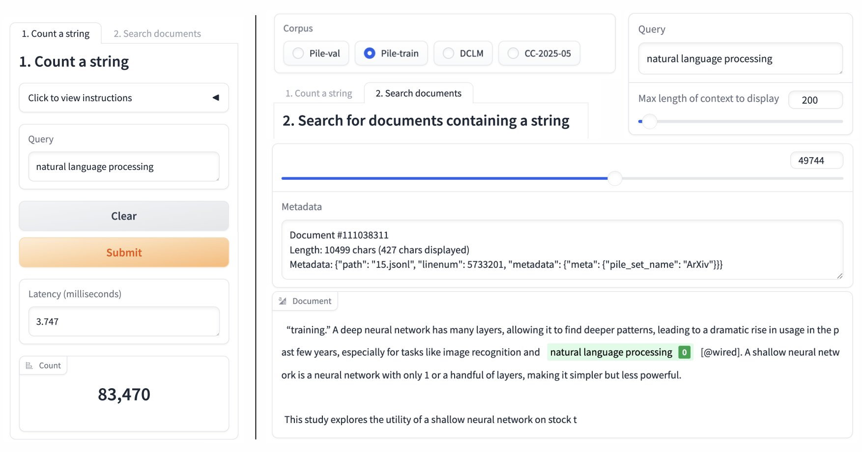
Figure 5: The web interface of infini-gram mini. Left: counting a string. Right: retrieving documents.

图 5：infini-gram mini 的 Web 界面。左： 计数字符串。右： 取回文档。

Appendix E Details for Benchmarks in Contamination Analysis

附录 E 污染分析所用基准细节

Table 5shows the benchmarks we analyze under each category with citation and source.

表 5 按类别列出所分析基准及引用与来源。

Benchmark	Citation	Source
Knowledge and Reasoning
MMLU	Hendrycks et al. 2021	https://huggingface.co/datasets/cais/mmlu
MMLU-Pro	Wang et al. 2024	https://huggingface.co/datasets/TIGER-Lab/MMLU-Pro
BigBenchHard	Suzgun et al. 2022	https://github.com/suzgunmirac/BIG-Bench-Hard/tree/main/bbh
AGIEval	Zhong et al. 2023	https://github.com/ruixiangcui/AGIEval/tree/main/data/v1_1
GPQA	Rein et al. 2023	https://huggingface.co/datasets/Idavidrein/gpqa
HLE	Phan et al. 2025	https://huggingface.co/datasets/cais/hle
Math
AIME-2024	of Problem Solving 2024	https://huggingface.co/datasets/Maxwell-Jia/AIME_2024
GSM8K	Cobbe et al. 2021	https://huggingface.co/datasets/openai/gsm8k
MATH-500	Lightman et al. 2023	https://huggingface.co/datasets/HuggingFaceH4/MATH-500
MGSM	Shi et al. 2022	https://huggingface.co/datasets/juletxara/mgsm
Code
HumanEval	Chen et al. 2021	https://huggingface.co/datasets/openai/openai_humaneval
HumanEval+	Liu et al. 2023	https://huggingface.co/datasets/evalplus/humanevalplus
LiveCodeBench	Jain et al. 2024	https://huggingface.co/datasets/livecodebench/code_generation
(code generation)
SWE-bench	Jimenez et al. 2024	https://huggingface.co/datasets/princeton-nlp/SWE-bench_Verified
MBPP	Austin et al. 2021	https://huggingface.co/datasets/google-research-datasets/mbpp
Commonsense Understanding
ARC-Challenge	Clark et al. 2018	https://huggingface.co/datasets/allenai/ai2_arc
ARC-Easy	Clark et al. 2018	https://huggingface.co/datasets/allenai/ai2_arc
CSQA	Talmor et al. 2019	https://huggingface.co/datasets/tau/commonsense_qa
HellaSwag	Zellers et al. 2019	https://huggingface.co/datasets/Rowan/hellaswag
Openbook QA	Mihaylov et al. 2018	https://huggingface.co/datasets/allenai/openbookqa
Social IQa	Sap et al. 2019	https://huggingface.co/datasets/allenai/social_i_qa
WinoGrande	Sakaguchi et al. 2019	https://huggingface.co/datasets/allenai/winogrande
Reading Comprehension
CoQA	Reddy et al. 2019	https://huggingface.co/datasets/stanfordnlp/coqa
SQuAD	Rajpurkar et al. 2016	https://huggingface.co/datasets/rajpurkar/squad

Table 5: Citation and source of each benchmark analyzed in this paper.

Benchmark	Citation	Source
Knowledge and Reasoning
MMLU	Hendrycks et al. 2021	https://huggingface.co/datasets/cais/mmlu
MMLU-Pro	Wang et al. 2024	https://huggingface.co/datasets/TIGER-Lab/MMLU-Pro
BigBenchHard	Suzgun et al. 2022	https://github.com/suzgunmirac/BIG-Bench-Hard/tree/main/bbh
AGIEval	Zhong et al. 2023	https://github.com/ruixiangcui/AGIEval/tree/main/data/v1_1
GPQA	Rein et al. 2023	https://huggingface.co/datasets/Idavidrein/gpqa
HLE	Phan et al. 2025	https://huggingface.co/datasets/cais/hle
Math
AIME-2024	of Problem Solving 2024	https://huggingface.co/datasets/Maxwell-Jia/AIME_2024
GSM8K	Cobbe et al. 2021	https://huggingface.co/datasets/openai/gsm8k
MATH-500	Lightman et al. 2023	https://huggingface.co/datasets/HuggingFaceH4/MATH-500
MGSM	Shi et al. 2022	https://huggingface.co/datasets/juletxara/mgsm
Code
HumanEval	Chen et al. 2021	https://huggingface.co/datasets/openai/openai_humaneval
HumanEval+	Liu et al. 2023	https://huggingface.co/datasets/evalplus/humanevalplus
LiveCodeBench	Jain et al. 2024	https://huggingface.co/datasets/livecodebench/code_generation
(code generation)
SWE-bench	Jimenez et al. 2024	https://huggingface.co/datasets/princeton-nlp/SWE-bench_Verified
MBPP	Austin et al. 2021	https://huggingface.co/datasets/google-research-datasets/mbpp
Commonsense Understanding
ARC-Challenge	Clark et al. 2018	https://huggingface.co/datasets/allenai/ai2_arc
ARC-Easy	Clark et al. 2018	https://huggingface.co/datasets/allenai/ai2_arc
CSQA	Talmor et al. 2019	https://huggingface.co/datasets/tau/commonsense_qa
HellaSwag	Zellers et al. 2019	https://huggingface.co/datasets/Rowan/hellaswag
Openbook QA	Mihaylov et al. 2018	https://huggingface.co/datasets/allenai/openbookqa
Social IQa	Sap et al. 2019	https://huggingface.co/datasets/allenai/social_i_qa
WinoGrande	Sakaguchi et al. 2019	https://huggingface.co/datasets/allenai/winogrande
Reading Comprehension
CoQA	Reddy et al. 2019	https://huggingface.co/datasets/stanfordnlp/coqa
SQuAD	Rajpurkar et al. 2016	https://huggingface.co/datasets/rajpurkar/squad

表 5：本文分析的各基准引用与来源。

Appendix F Detailed Benchmark Contamination Result

附录 F 详细基准污染结果

Table 6reports the number of suspicious and dirty entries of each benchmark.

表 6 报告各基准可疑与脏条目数量。

Benchmark	Test Set	Pile-train	DCLM-baseline	CC-2025-05
	Size	Suspicious	Dirty	Suspicious	Dirty	Suspicious	Dirty
Knowledge and Reasoning
MMLU	1000	57	133	142	277	122	135
MMLU-Pro	1000	35	59	77	162	31	81
BigBenchHard	1000	7	0	54	1	357	14
AGIEval	1000	45	8	155	31	107	27
GPQA	448	1	0	5	0	6	4
HLE	881	3	0	6	0	8	0
Math
AIME-2024	30	2	0	4	0	13	3
GSM8K	1000	1	0	5	4	33	76
MATH-500	500	9	3	48	16	26	3
MGSM	250	0	0	2	0	9	14
Code
HumanEval	164	1	0	1	0	14	0
HumanEval+	164	1	0	1	0	14	0
LiveCodeBench	880	2	0	2	0	188	0
SWE-bench	500	5	0	26	0	29	1
MBPP	500	16	0	64	2	87	5
Commonsense Understanding
ARC-Challenge	1000	6	14	4	341	18	119
ARC-Easy	1000	15	15	5	317	31	54
CSQA	1000	0	1	1	10	1	1
HellaSwag	1000	27	0	341	0	36	0
OpenbookQA	500	2	54	3	78	5	73
Social IQa	1000	0	0	2	5	2	2
WinoGrande	1000	2	0	0	0	0	0
Reading Comprehension
CoQA	500	189	40	188	92	121	37
SQuAD	1000	16	28	9	401	11	27

Table 6: Detailed benchmark contamination results. For test sets with more than 1000 entries, we randomly downsample to 1000.

Benchmark	Test Set	Pile-train	DCLM-baseline	CC-2025-05
	Size	Suspicious	Dirty	Suspicious	Dirty	Suspicious	Dirty
Knowledge and Reasoning
MMLU	1000	57	133	142	277	122	135
MMLU-Pro	1000	35	59	77	162	31	81
BigBenchHard	1000	7	0	54	1	357	14
AGIEval	1000	45	8	155	31	107	27
GPQA	448	1	0	5	0	6	4
HLE	881	3	0	6	0	8	0
Math
AIME-2024	30	2	0	4	0	13	3
GSM8K	1000	1	0	5	4	33	76
MATH-500	500	9	3	48	16	26	3
MGSM	250	0	0	2	0	9	14
Code
HumanEval	164	1	0	1	0	14	0
HumanEval+	164	1	0	1	0	14	0
LiveCodeBench	880	2	0	2	0	188	0
SWE-bench	500	5	0	26	0	29	1
MBPP	500	16	0	64	2	87	5
Commonsense Understanding
ARC-Challenge	1000	6	14	4	341	18	119
ARC-Easy	1000	15	15	5	317	31	54
CSQA	1000	0	1	1	10	1	1
HellaSwag	1000	27	0	341	0	36	0
OpenbookQA	500	2	54	3	78	5	73
Social IQa	1000	0	0	2	5	2	2
WinoGrande	1000	2	0	0	0	0	0
Reading Comprehension
CoQA	500	189	40	188	92	121	37
SQuAD	1000	16	28	9	401	11	27

表 6：详细基准污染结果。测试集超过 1000 条时随机下采样至 1000。

Appendix G Contamination Examples

附录 G 污染示例

Figure 6to Figure 12 shows example dirty entries in seven benchmarks and its contamination source retrieved from one of three corpus using infini-gram mini. We also present the original webpage that is responsible for the contamination.

图 6 至图 12 展示七个基准中的脏条目示例，以及用 infini-gram mini 从三大语料之一取回的污染来源；并给出造成污染的原始网页。

(a) Left upper: An entry in the AIME-2024 benchmark. Right: A document contaminating this entry, retrieved from CC-2025-05 by infini-gram mini. This example belongs to Category 1, where the correct answer can be found in the document.

(a) 左上： AIME-2024 基准条目。右： 由 infini-gram mini 从 CC-2025-05 取回的污染该条目的文档。属类别 1，文档中可找到正确答案。

(a) Left upper: An entry in the MMLU benchmark. Right: A document contaminating this entry, retrieved from CC-2025-05 by infini-gram mini. This example belongs to Category 1, where the correct answer presents (though choices are not in the exact same order).

(a) 左上： MMLU 基准条目。右： 从 CC-2025-05 取回的污染文档。属类别 1，正确答案出现（选项顺序不完全相同）。

(a) Left upper: An entry in the SWE-bench benchmark. Right: A document contaminating this entry, retrieved from CC-2025-05 by infini-gram mini. This example is Category 3, where only question appears but not the answer.

(a) 左上： SWE-bench 基准条目。右： 从 CC-2025-05 取回的污染文档。属类别 3，仅问题出现、无答案。

(a) Left bottom: An entry in the GPQA benchmark. Right: A document contaminating this entry, retrieved from CC-2025-05 by infini-gram mini. This example belongs to Category 3, where only the question appears, not the answers.

(a) 左下： GPQA 基准条目。右： 从 CC-2025-05 取回的污染文档。属类别 3，仅问题出现、无答案。

(a) Left bottom: An entry in the GSM8K benchmark. Right: A document contaminating this entry, retrieved from CC-2025-05 by infini-gram mini. This example is Category 3 because the correct answer is not present.

(a) 左下： GSM8K 基准条目。右： 从 CC-2025-05 取回的污染文档。因正确答案未出现，属类别 3。

(a) Left bottom: An entry in the BigBenchHard benchmark. Right: A document contaminating this entry, retrieved from CC-2025-05 by infini-gram mini. This example is Category 3 because the correct answer is not present.

(a) 左下： BigBenchHard 基准条目。右： 从 CC-2025-05 取回的污染文档。因正确答案未出现，属类别 3。

(a) Left bottom: An entry in the OpenbookQA benchmark. Right: A document contaminating this entry, retrieved from Pile-train by infini-gram mini. This example is Category 2 where the correct answer appears in natural language.

(a) 左下： OpenbookQA 基准条目。右： 从 Pile-train 取回的污染文档。属类别 2，正确答案以自然语言出现。

Appendix H Dirty Entry Categorization using LLM-as-a-judge

附录 H 用 LLM-as-a-judge 归类脏条目

We use gpt-4o-mini to categorize all dirty entries into one of four categories described in §4.3. For each dirty entry, we extract the 50-character substring that has least occurrence in the corpus. We then retrieve text snippet with context length of 400 characters (850 characters in total). We prompt gpt-4o-mini by providing both the dirty entry and the text snippet and let the model decide which category the dirty entry belongs. We use the following prompt:

我们用 gpt-4o-mini 将全部脏条目归入 §4.3 所述四类。对每个脏条目，抽取在语料中出现最少的 50 字符子串，再取回上下文总长约 850 字符（含 400 字符上下文）的文本片段。向模型同时提供脏条目与片段并判定类别。所用提示如下：

You are an expert in evaluating benchmark contamination. Given an entry and detected overlap in the corpus, categorize how the entry is contaminated in corpus into one of four categories: 1. You can find exact match of question stem and the correct answer (correct choice if multiple choices, or answer matching exactly the answer field) in corpus. 2. You can find exact match of question stem, and the correct answer appears, though not in exact match. 3. You can find exact match of question stem, but you cannot find the correct answer in any form. 4. False positive Output only the category number.

你是评估基准污染的专家。给定条目及语料中检测到的重叠，将该条目在语料中的污染方式归入以下四类之一：1. 可在语料中找到题干与正确答案的精确匹配（多选则为正确选项，或与答案字段完全一致）。2. 可找到题干精确匹配，正确答案出现但非精确匹配。3. 可找到题干精确匹配，但任何形式的正确答案都找不到。4. 假阳性。只输出类别编号。

Appendix I Interface of the Benchmark Contamination Monitoring System

附录 I 基准污染监测系统界面

Figure 13shows the interface of the system. It consists of two tabs: (1) Benchmark Contamination Bulletin, and (2) submission page for community to contribute. Benchmarks analyzed in this paper are reported in “core” table, and submitted benchmarks will be added to “community” table.

图 13 展示系统界面，含两个标签页：(1) 基准污染公告板；(2) 社区投稿页。本文分析的基准列在 “core” 表，提交的基准加入 “community” 表。

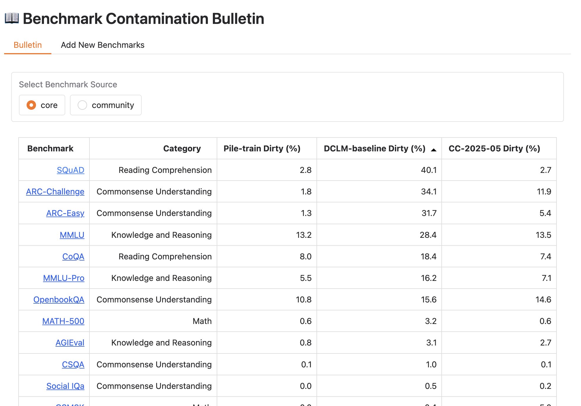
Figure 13: Upper: A screenshot of our online Benchmark Contamination Bulletin. Lower: We invite the community to add new benchmarks or upload new ones for contamination analysis, which will be added to the bulletin.

图 13：上： 在线基准污染公告板截图。下： 邀请社区添加或上传新基准做污染分析，结果将加入公告板。

Appendix J License of Corpora Used in the Paper

附录 J 本文所用语料许可

Pile and DCLM are licensed under the MIT License. Common Crawl is licensed under its customized Limited License. We followed the listed intended use.

Pile 与 DCLM 采用 MIT License。Common Crawl 采用其定制 Limited License。我们遵循所列预期用途。