Quo Vadis, Action Recognition? A New Model and the Kinetics Dataset
Quo Vadis, Action Recognition? A New Model and the Kinetics Dataset
何去何从,动作识别?一种新模型与 Kinetics 数据集
João Carreira†
joaoluis@google.com
Andrew Zisserman†,∗
zisserman@google.com
†DeepMind ∗Department of Engineering Science, University of Oxford
Abstract
摘要
The paucity of videos in current action classification datasets (UCF-101 and HMDB-51) has made it difficult to identify good video architectures, as most methods obtain similar performance on existing small-scale benchmarks. This paper re-evaluates state-of-the-art architectures in light of the new Kinetics Human Action Video dataset. Kinetics has two orders of magnitude more data, with 400 human action classes and over 400 clips per class, and is collected from realistic, challenging YouTube videos. We provide an analysis on how current architectures fare on the task of action classification on this dataset and how much performance improves on the smaller benchmark datasets after pre-training on Kinetics.
当前动作分类数据集(UCF-101 和 HMDB-51)中的视频数量很少,这让人很难判断怎样的视频结构更好,因为多数方法在现有的小规模基准上表现接近。本文借助新的 Kinetics 人类动作视频数据集,重新评估了当时最先进的一类结构。Kinetics 的数据量高出约两个数量级,包含 400 个人类动作类别、每类超过 400 条片段,并采集自真实、有难度的 YouTube 视频。我们分析了现有结构在这一数据集上的动作分类表现,以及在 Kinetics 上预训练之后,它们在更小基准上的性能能提高多少。
We also introduce a new Two-Stream Inflated 3D ConvNet (I3D) that is based on 2D ConvNet inflation: filters and pooling kernels of very deep image classification ConvNets are expanded into 3D, making it possible to learn seamless spatio-temporal feature extractors from video while leveraging successful ImageNet architecture designs and even their parameters. We show that, after pre-training on Kinetics, I3D models considerably improve upon the state-of-the-art in action classification, reaching 80.2% on HMDB-51 and 97.9% on UCF-101.
我们还提出一种新的双流膨胀三维卷积网络(Two-Stream Inflated 3D ConvNet,I3D),其基础是把二维 ConvNet 加以膨胀:把很深的图像分类 ConvNet 中的滤波核和池化核扩展到三维,从而可以在视频上学习连贯的时空特征提取器,同时借用已经在 ImageNet 上验证过的结构设计,甚至直接借用它们的参数。我们表明,在 Kinetics 上预训练之后,I3D 模型在动作分类上明显超过当时最好结果,在 HMDB-51 上达到 80.2%,在 UCF-101 上达到 97.9%。
1. Introduction
1. 引言
One of the unexpected benefits of the ImageNet challenge has been the discovery that deep architectures trained on the 1000 images of 1000 categories, can be used for other tasks and in other domains. One of the early examples of this was using the fc7 features from a network trained on ImageNet for the PASCAL VOC classification and detection challenge [10]. Furthermore, improvements in the deep architecture, changing from AlexNet to VGG-16, immediately fed through to commensurate improvements in the PASCAL VOC performance [23]. Since then, there have been numerous examples of ImageNet trained architectures warm starting or sufficing entirely for other tasks, e.g. segmentation, depth prediction, pose estimation, action classification.
ImageNet 挑战赛带来的一个意外收获是:在 1000 类、每类约 1000 张图像上训练出的深度结构,也可以用于其他任务和其他领域。较早的例子之一,是把在 ImageNet 上训练的网络的 fc7 特征用到 PASCAL VOC 分类与检测挑战中 [10]。此后,深度结构从 AlexNet 换成 VGG-16,PASCAL VOC 上的成绩也随即有了相应提高 [23]。从那以后,用 ImageNet 训练好的结构来热启动、甚至直接胜任其他任务的例子已经很多,例如分割、深度预测、姿态估计、动作分类。
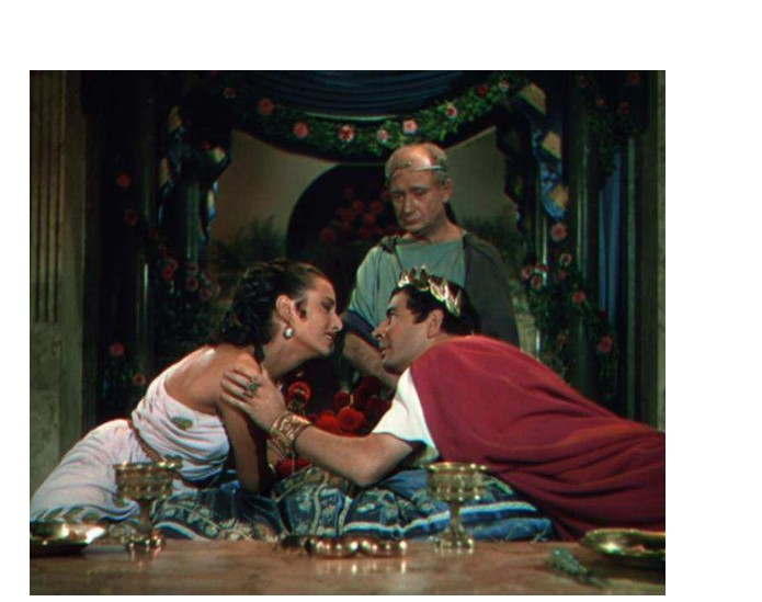
Figure 1. A still from ‘Quo Vadis’ (1951). Where is this going? Are these actors about to kiss each other, or have they just done so? More importantly, where is action recognition going? Actions can be ambiguous in individual frames, but the limitations of existing action recognition datasets has meant that the best-performing video architectures do not depart significantly from single-image analysis, where they rely on powerful image classifiers trained on ImageNet. In this paper we demonstrate that video models are best pre-trained on videos and report significant improvements by using spatio-temporal classifiers pre-trained on Kinetics, a freshly collected, large, challenging human action video dataset.
图 1. 电影《Quo Vadis》(1951)中的一帧。故事接下来会怎样?这两位演员是正要接吻,还是刚刚吻过?更重要的是,动作识别接下来会走向哪里?单个帧里的动作常常是含糊的;可是现有动作识别数据集的局限,使得表现最好的视频结构并没有真正离开单图分析,它们仍然依赖在 ImageNet 上训练出的强大图像分类器。本文表明,视频模型最好在视频上预训练,并报告:使用在新收集的、大规模且有难度的人类动作视频数据集 Kinetics 上预训练的时空分类器,可以带来显著提升。
In the video domain, it is an open question whether training an action classification network on a sufficiently large dataset, will give a similar boost in performance when applied to a different temporal task or dataset. The challenges of building video datasets has meant that most popular benchmarks for action recognition are small, having on the order of 10k videos.
在视频领域,一个尚未解决的问题是:如果在足够大的数据集上训练动作分类网络,再把它用到另一种时间性任务或另一份数据上,是否也会出现类似的性能提升。构建视频数据集的困难,使得目前最常用的动作识别基准仍然很小,大约只有一万条视频的量级。
In this paper we aim to provide an answer to this question using the new Kinetics Human Action Video Dataset [16], which is two orders of magnitude larger than previous datasets, HMDB-51 [18] and UCF-101 [27]. Kinetics has 400 human action classes with more than 400 examples for each class, each from a unique YouTube video.
本文希望借助新的 Kinetics 人类动作视频数据集 [16] 来回答这个问题。它比先前的 HMDB-51 [18] 和 UCF-101 [27] 大约大两个数量级。Kinetics 有 400 个人类动作类别,每类有 400 条以上样本,且每条样本来自不同的 YouTube 视频。
Our experimental strategy is to reimplement a number of representative neural network architectures from the literature, and then analyze their transfer behavior by first pre-training each one on Kinetics and then fine-tuning each on HMDB-51 and UCF-101. The results suggest that there is always a boost in performance by pre-training, but the extent of the boost varies significantly with the type of architecture. Based on these findings, we introduce a new model that has the capacity to take advantage of pre-training on Kinetics, and can achieves a high performance. The model termed a “Two-Stream Inflated 3D ConvNets” (I3D), builds upon state-of-the-art image classification architectures, but inflates their filters and pooling kernels (and optionally their parameters) into 3D, leading to very deep, naturally spatio-temporal classifiers. An I3D model based on Inception-v1 [13] obtains performance far exceeding the state-of-the-art, after pre-training on Kinetics.
我们的实验策略是:复现文献中若干有代表性的神经网络结构,先在 Kinetics 上对每一个做预训练,再在 HMDB-51 和 UCF-101 上微调,从而分析它们的迁移行为。结果表明,预训练总会带来提升,但提升幅度随结构类型明显不同。基于这些发现,我们提出一种有能力充分利用 Kinetics 预训练、并能达到很高性能的新模型。这一模型称为“双流膨胀三维卷积网络”(Two-Stream Inflated 3D ConvNets,I3D),它建立在当时最先进的图像分类结构之上,但把滤波核和池化核(以及可选的参数)膨胀到三维,从而得到很深、并且天生是时空的分类器。基于 Inception-v1 [13] 的 I3D 模型在 Kinetics 预训练之后,性能远超当时最好结果。
In our model comparisons, we did not consider more classic approaches such as bag-of-visual-words representations [6, 19, 21, 30]. However, the Kinetics dataset is publicly available, so others can use it for such comparisons.
在模型比较中,我们没有纳入词袋(bag-of-visual-words)这类更经典的方法 [6, 19, 21, 30]。不过 Kinetics 数据集是公开的,其他人可以用它来做这类比较。
The next section outlines the set of implemented action classification models. Section 3 gives an overview of the Kinetics dataset. Section 4 reports the performance of models on previous benchmarks and on Kinetics, and section 5 studies how well the features learned on Kinetics transfer to different datasets. The paper concludes with a discussion of the results.
下一节概述我们所实现的动作分类模型。第 3 节介绍 Kinetics 数据集。第 4 节报告这些模型在先前基准和 Kinetics 上的表现,第 5 节研究在 Kinetics 上学到的特征迁移到其他数据集时效果如何。论文最后对结果进行讨论。
2. Action Classification Architectures
2. 动作分类结构
While the development of image representation architectures has matured quickly in recent years, there is still no clear front running architecture for video. Some of the major differences in current video architectures are whether the convolutional and layers operators use 2D (image-based) or 3D (video-based) kernels; whether the input to the network is just an RGB video or it also includes pre-computed optical flow; and, in the case of 2D ConvNets, how information is propagated across frames, which can be done either using temporally-recurrent layers such as LSTMs, or feature aggregation over time.
近年来图像表示结构已经很快成熟,但视频领域仍没有明显领先的结构。当前视频结构的主要差别包括:卷积及各类算子使用的是二维(基于图像)还是三维(基于视频)核;网络输入只是 RGB 视频,还是同时包含预先计算的光流;以及在二维 ConvNet 的情形下,信息如何在帧之间传递——既可以借助 LSTM 这类时间循环层,也可以做跨时间的特征聚合。
In this paper we compare and study a subset of models that span most of this space. Among 2D ConvNet methods, we consider ConvNets with LSTMs on top [5, 34], and two-stream networks with two different types of stream fusion [8, 25]. We also consider a 3D ConvNet [14, 28]: C3D [29].
本文比较并研究了覆盖这一设计空间大部分位置的一组模型。在二维 ConvNet 方法中,我们考虑在顶部加 LSTM 的 ConvNet [5, 34],以及两种不同融合方式的双流网络 [8, 25]。我们也考虑一种三维 ConvNet [14, 28]:C3D [29]。
As the main technical contribution, we introduce Two-Stream Inflated 3D ConvNets (I3D). Due to the high-dimensionality of their parameterization and the lack of labeled video data, previous 3D ConvNets have been relatively shallow (up to 8 layers). Here we make the observation that very deep image classification networks, such as Inception [13], VGG-16 [26] and ResNet [12], can be trivially inflated into spatio-temporal feature extractors, and that their pre-trained weights provide a valuable initialization. We also find that a two-stream configuration is still useful.
作为主要技术贡献,我们提出双流膨胀三维卷积网络(I3D)。由于参数维度高、标注视频又少,以往的三维 ConvNet 相对较浅(最多约 8 层)。我们观察到,Inception [13]、VGG-16 [26] 和 ResNet [12] 这类很深的图像分类网络,可以很直接地膨胀成时空特征提取器,而且它们的预训练权重是很有价值的初始化。我们也发现,双流配置仍然有用。
A graphical overview of the five types of architectures we evaluate is shown in figure 2 and the specification of their temporal interfaces is given in table 1.
图 2 给出了我们评估的五类结构的示意图,表 1 给出了它们时间接口的具体设定。
Many of these models (all but C3D) have an Imagenet pre-trained model as a subcomponent. Our experimental strategy assumes a common ImageNet pre-trained image classification architecture as back bone, and for this we chose Inception-v1 with batch normalization [13], and morph it in different ways. The expectation is that with this back bone in common, we will be able to tease apart those changes that benefit action classification the most.
这些模型中的多数(C3D 除外)都以一个 ImageNet 预训练模型作为子模块。我们的实验策略假定大家都用同一个在 ImageNet 上预训练的图像分类结构作为骨干,为此我们选择带批量归一化的 Inception-v1 [13],再以不同方式改造它。我们期望,在骨干相同的前提下,能够把那些对动作分类最有帮助的改动分离出来。
2.1. The Old I: ConvNet+LSTM
2.1. 旧方法 I:ConvNet+LSTM
The high performance of image classification networks makes it appealing to try to reuse them with as minimal change as possible for video. This can be achieved by using them to extract features independently from each frame then pooling their predictions across the whole video [15]. This is in the spirit of bag of words image modeling approaches [19, 21, 30]; but while convenient in practice, it has the issue of entirely ignoring temporal structure (e.g. models can’t potentially distinguish opening from closing a door).
图像分类网络的高性能,使人很想尽量少改动就把它们用到视频上。一种做法是对每一帧独立提取特征,再把整段视频上的预测做池化 [15]。这和词袋式的图像建模思路类似 [19, 21, 30];实践中很方便,但完全忽略了时间结构(例如,模型可能无法区分开门和关门)。
In theory, a more satisfying approach is to add a recurrent layer to the model [5, 34], such as an LSTM, which can encode state, and capture temporal ordering and long range dependencies. We position an LSTM layer with batch normalization (as proposed by Cooijmans et al. [4]) after the last average pooling layer of Inception-V1, with 512 hidden units. A fully connected layer is added on top for the classifier.
从道理上讲,更令人满意的做法是给模型加上循环层 [5, 34],例如 LSTM,它能够编码状态,并捕捉时间顺序和长程依赖。我们在 Inception-V1 的最后一层平均池化之后,放置一个带批量归一化的 LSTM 层(采用 Cooijmans 等人 [4] 的做法),隐单元数为 512,再在其上加一个全连接层作为分类器。
The model is trained using cross-entropy losses on the outputs at all time steps. During testing we consider only the output on the last frame. Input video frames are subsampled by keeping one out of every 5, from an original 25 frames-per-second stream. The full temporal footprint of all models is given in table 1.
训练时,对所有时间步的输出都使用交叉熵损失。测试时只考虑最后一帧的输出。输入视频帧从原来的 25 帧/秒中每隔 5 帧保留 1 帧。各模型完整的时间覆盖范围见表 1。
2.2. The Old II: 3D ConvNets
2.2. 旧方法 II:三维 ConvNet
3D ConvNets seem like a natural approach to video modeling, and are just like standard convolutional networks, but with spatio-temporal filters. They have been explored several times, previously [14, 28, 29]. They have a very important characteristic: they directly create hierarchical representations of spatio-temporal data. One issue with these models is that they have many more parameters than 2D ConvNets because of the additional kernel dimension, and this makes them harder to train. Also, they seem to preclude the benefits of ImageNet pre-training, and consequently previous work has defined relatively shallow custom architectures and trained them from scratch [14, 15, 28, 29]. Results on benchmarks have shown promise but have not been competitive with state-of-the-art, making this type of models a good candidate for evaluation on our larger dataset.
三维 ConvNet 看起来是视频建模的自然选择,它和普通卷积网络很像,只是滤波核是时空的。这类模型此前已被多次探索 [14, 28, 29]。它们有一个非常重要的特点:能够直接建立时空数据的层次化表示。一个问题是,由于多了核的时间维,参数量比二维 ConvNet 多很多,因而更难训练。它们似乎也难以享受 ImageNet 预训练的好处,因此以往工作往往设计相对较浅的定制结构,并从零开始训练 [14, 15, 28, 29]。在已有基准上的结果有一定前景,但还不足以与当时最好方法竞争,所以这类模型很适合放到我们这份更大的数据上再评估一次。
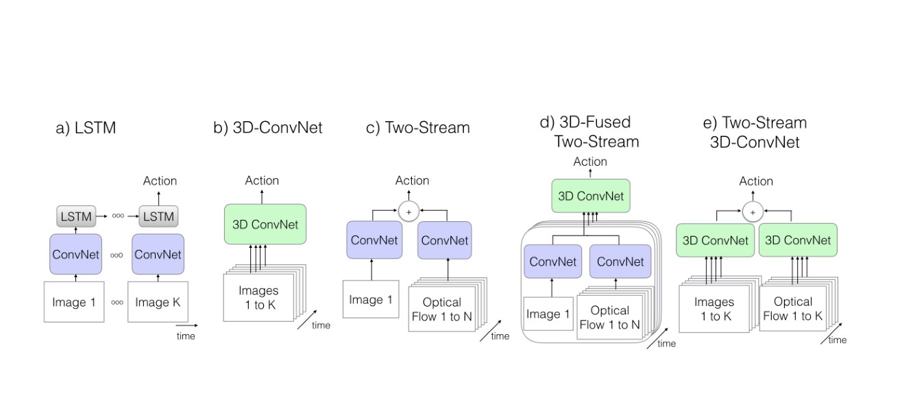
Figure 2. Video architectures considered in this paper. K stands for the total number of frames in a video, whereas N stands for a subset of neighboring frames of the video.
图 2. 本文考虑的视频结构。K 表示一段视频的总帧数,N 表示其中一组相邻帧。
For this paper we implemented a small variation of C3D [29], which has 8 convolutional layers, 5 pooling layers and 2 fully connected layers at the top. The inputs to the model are short 16-frame clips with 112 × 112-pixel crops as in the original implementation. Differently from [29] we used batch normalization after all convolutional and fully connected layers. Another difference to the original model is in the first pooling layer, we use a temporal stride of 2 instead of 1, which reduces the memory footprint and allows for bigger batches – this was important for batch normalization (especially after the fully connected layers, where there is no weight tying). Using this stride we were able to train with 15 videos per batch per GPU using standard K40 GPUs.
本文实现了一个与 C3D [29] 接近的小变体,它有 8 个卷积层、5 个池化层,顶部还有 2 个全连接层。与原实现一样,模型输入是短的 16 帧片段,并裁成 112 × 112 像素。与 [29] 不同的是,我们在所有卷积层和全连接层之后都使用了批量归一化。另一处不同是第一个池化层:时间步长取 2 而不是 1,以减小显存占用并允许更大的批量——这对批量归一化很重要(尤其是在没有权值共享的全连接层之后)。采用这一步长后,我们能够在标准的 K40 GPU 上按每块 GPU 每批 15 段视频来训练。
2.3. The Old III: Two-Stream Networks
2.3. 旧方法 III:双流网络
LSTMs on features from the last layers of ConvNets can model high-level variation, but may not be able to capture fine low-level motion which is critical in many cases. It is also expensive to train as it requires unrolling the network through multiple frames for backpropagation-through-time.
把 LSTM 接在 ConvNet 最后几层的特征上,可以建模高层变化,但未必能抓住许多情形里至关重要的细粒度低层运动。而且训练代价也高,因为反向传播通过时间时需要把网络在多帧上展开。
A different, very practical approach, introduced by Simonyan and Zisserman [25], models short temporal snapshots of videos by averaging the predictions from a single RGB frame and a stack of 10 externally computed optical flow frames, after passing them through two replicas of an ImageNet pre-trained ConvNet. The flow stream has an adapted input convolutional layer with twice as many input channels as flow frames (because flow has two channels, horizontal and vertical), and at test time multiple snapshots are sampled from the video and the action prediction is averaged. This was shown to get very high performance on existing benchmarks, while being very efficient to train and test.
Simonyan 和 Zisserman [25] 提出了另一种非常实用的做法:把单张 RGB 帧和一叠 10 帧外部计算的光流,分别送入两个 ImageNet 预训练 ConvNet 的副本,再把预测平均,以此来建模视频的短时快照。光流这一路的输入卷积层经过改造,输入通道数是光流帧数的两倍(因为光流有水平和垂直两个通道);测试时从视频中采样多个快照,再对动作预测取平均。这一方法在已有基准上表现很高,训练和测试也都很高效。
A recent extension [8] fuses the spatial and flow streams after the last network convolutional layer, showing some improvement on HMDB while requiring less test time augmentation (snapshot sampling). Our implementation follows this paper approximately using Inception-V1. The inputs to the network are 5 consecutive RGB frames sampled 10 frames apart, as well as the corresponding optical flow snippets. The spatial and motion features before the last average pooling layer of Inception-V1 (5 × 7 × 7 feature grids, corresponding to time, x and y dimensions) are passed through a 3 × 3 × 3 3D convolutional layer with 512 output channels, followed by a 3 × 3 × 3 3D max-pooling layer and through a final fully connected layer. The weights of these new layers are initialized with Gaussian noise.
最近的一个扩展 [8] 在网络最后一个卷积层之后融合空间流和光流,在 HMDB 上有所提升,同时减少了测试时的增强(快照采样)。我们的实现大致跟随该文,骨干采用 Inception-V1。网络输入是间隔 10 帧采样的 5 张连续 RGB 帧,以及对应的光流片段。Inception-V1 最后一层平均池化之前的空间与运动特征(5 × 7 × 7 的特征网格,分别对应时间、x 和 y)被送入一个输出 512 通道的 3 × 3 × 3 三维卷积层,再经过 3 × 3 × 3 三维最大池化,最后接一个全连接层。这些新层的权重用高斯噪声初始化。
Both models, the original two-stream and the 3D fused version, are trained end-to-end (including the two-stream averaging process in the original model).
原来的双流模型以及三维融合版本,都是端到端训练的(包括原模型中的双流平均过程)。
2.4. The New: Two-Stream Inflated 3D ConvNets
2.4. 新方法:双流膨胀三维 ConvNet
With this architecture, we show how 3D ConvNets can benefit from ImageNet 2D ConvNet designs and, optionally, from their learned parameters. We also adopt a two-stream configuration here – it will be shown in section 4 that while 3D ConvNets can directly learn about temporal patterns from an RGB stream, their performance can still be greatly improved by including an optical-flow stream.
借助这一结构,我们说明三维 ConvNet 如何能够受益于 ImageNet 上的二维 ConvNet 设计,并且可选地受益于它们已经学到的参数。这里我们同样采用双流配置——第 4 节将会表明:虽然三维 ConvNet 能够直接从 RGB 流中学习时间模式,但再加入光流仍然可以大大提高性能。
Inflating 2D ConvNets into 3D
把二维 ConvNet 膨胀成三维
A number of very successful image classification architectures have been developed over the years, in part through painstaking trial and error. Instead of repeating the process for spatio-temporal models we propose to simply convert successful image (2D) classification models into 3D ConvNets. This can be done by starting with a 2D architecture, and inflating all the filters and pooling kernels – endowing them with an additional temporal dimension. Filters are typically square and we just make them cubic – N × N filters become N × N × N.
这些年来已经出现了不少非常成功的图像分类结构,其中一部分是靠大量试错得来的。我们不想在时空模型上重复这一过程,于是提议把已经成功的图像(二维)分类模型直接转换成三维 ConvNet。做法是从二维结构出发,把所有滤波核和池化核膨胀,给它们增加一个时间维。滤波核通常是方形的,我们把它们变成立方体—— 的核变成 。
Bootstrapping 3D filters from 2D Filters
从二维滤波核引导三维滤波核
Besides the architecture, one may also want to bootstrap parameters from the pre-trained ImageNet models. To do this, we observe that an image can be converted into a (boring) video by copying it repeatedly into a video sequence. The 3D models can then be implicitly pre-trained on ImageNet, by satisfying what we call the boring-video fixed point: the pooled activations on a boring video should be the same as on the original single-image input. This can be achieved, thanks to linearity, by repeating the weights of the 2D filters N times along the time dimension, and rescaling them by dividing by N. This ensures that the convolutional filter response is the same. Since the outputs of convolutional layers for boring videos are constant in time, the outputs of pointwise non-linearity layers and average and max-pooling layers are the same as for the 2D case, and hence the overall network response respects the boring-video fixed point.
除了结构,人们往往还希望从预训练的 ImageNet 模型中引导参数。为此我们观察到,只要把同一张图反复复制成一段视频,就可以把一张图像变成一段(乏味的)视频。三维模型于是可以隐式地在 ImageNet 上预训练,只需满足我们所说的“乏味视频不动点”:这段乏味视频上的池化激活,应当与原来单张图像输入上的激活相同。由于线性性,这可以通过把二维滤波核的权重沿时间维重复 次,再除以 来实现。这样可以保证卷积滤波的响应相同。因为乏味视频上卷积层的输出在时间上是恒定的,逐点非线性层以及平均池化和最大池化的输出也与二维情形相同,从而整个网络的响应满足乏味视频不动点。
Pacing receptive field growth in space, time and network depth
在空间、时间和网络深度上安排感受野的增长
The boring video fixed-point leaves ample freedom on how to inflate pooling operators along the time dimension and on how to set convolutional/pooling temporal stride – these are the primary factors that shape the size of feature receptive fields. Virtually all image models treat the two spatial dimensions (horizontal and vertical) equally – pooling kernels and strides are the same. This is quite natural and means that features deeper in the networks are equally affected by image locations increasingly far away in both dimensions. A symmetric receptive field is however not necessarily optimal when also considering time – this should depend on frame rate and image dimensions. If it grows too quickly in time relative to space, it may conflate edges from different objects breaking early feature detection, while if it grows too slowly, it may not capture scene dynamics well.
乏味视频不动点在如何沿时间膨胀池化算子、以及如何设置卷积/池化的时间步长上,仍留下很大自由——而这些正是决定特征感受野大小的主要因素。几乎所有图像模型对两个空间维(水平和垂直)一视同仁,池化核和步长都相同。这很自然,也意味着网络越深的特征,会同样受到两个方向上越来越远的图像位置的影响。但一旦把时间也考虑进来,对称的感受野并不一定最优,这应当取决于帧率和图像尺寸。如果它在时间上相对空间增长过快,就可能把不同物体的边缘混在一起,破坏早期特征检测;如果增长过慢,又可能捕捉不好场景动态。
In Inception-v1, the first convolutional layer has stride 2, then there are four max-pooling layers with stride 2 and a 7 × 7 average-pooling layer preceding the last linear classification layer, besides the max-pooling layers in parallel Inception branches. In our experiments the input videos were processed at 25 frames per second; we found it helpful to not perform temporal pooling in the first two max-pooling layers (by using 1 × 3 × 3 kernels and stride 1 in time), while having symmetric kernels and strides in all other max-pooling layers. The final average pooling layer uses a 2×7×7 kernel. The overall architecture is shown in fig. 3. We train the model using 64-frame snippets and test using the whole videos, averaging predictions temporally.
在 Inception-v1 中,第一个卷积层的步长为 2,随后有四个步长为 2 的最大池化层,以及位于最后线性分类层之前的 7 × 7 平均池化层;此外,并行的 Inception 分支里还有最大池化层。我们的实验里,输入视频按 25 帧/秒处理;我们发现,前两个最大池化层不做时间池化(时间维使用 1 × 3 × 3 的核、步长为 1)是有帮助的,而其余最大池化层则使用对称的核和步长。最后的平均池化层使用 2×7×7 的核。整体结构见图 3。我们用 64 帧片段训练模型,测试时则使用整段视频,并对预测做时间平均。
Two 3D Streams
两条三维流
While a 3D ConvNet should be able to learn motion features from RGB inputs directly, it still performs pure feedforward computation, whereas optical flow algorithms are in some sense recurrent (e.g. they perform iterative optimization for the flow fields). Perhaps because of this lack of recurrence, experimentally we still found it valuable to have a two-stream configuration – shown in fig. 2, e) – with one I3D network trained on RGB inputs, and another on flow inputs which carry optimized, smooth flow information. We trained the two networks separately and averaged their predictions at test time.
三维 ConvNet 理应能够直接从 RGB 输入中学习运动特征,但它仍然只做纯前馈计算,而光流算法在某种意义上是循环的(例如,它们会对光流场做迭代优化)。也许正是因为缺少这种循环,我们在实验中仍然发现双流配置是有价值的——见图 2 的 e):一路 I3D 在 RGB 输入上训练,另一路在带有优化过的平滑光流信息的输入上训练。两路网络分开训练,测试时把它们的预测平均。
2.5. Implementation Details
2.5. 实现细节
All models but the C3D-like 3D ConvNet use ImageNet-pretrained Inception-V1 [13] as base network. For all architectures we follow each convolutional layer by a batch normalization [13] layer and a ReLU activation function, except for the last convolutional layers which produce the class scores for each network.
除了类似 C3D 的三维 ConvNet 之外,所有模型都以 ImageNet 预训练的 Inception-V1 [13] 作为基础网络。对所有结构,我们在每个卷积层之后接批量归一化 [13] 层和 ReLU 激活,最后产生各类得分的卷积层除外。
Training on videos used standard SGD with momentum set to 0.9 in all cases, with synchronous parallelization across 32 GPUs for all models except the 3D ConvNets which receive a large number of input frames and hence require more GPUs to form large batches – we used 64 GPUs for these. We trained models on miniKinetics for up to 35k steps, and for 110k steps on Kinetics, with a 10x reduction of learning rate when validation loss saturated. We tuned the learning rate hyperparameter on the validation set of miniKinetics. Models were trained for up to 5k steps on UCF-101 and HMDB-51 using a similar learning rate adaptation procedure as for Kinetics but using just 16 GPUs. All the models were implemented in TensorFlow [1].
视频上的训练一律使用标准 SGD,动量设为 0.9;除三维 ConvNet 外,所有模型都在 32 块 GPU 上同步并行。三维 ConvNet 因为输入帧数多,需要更多 GPU 才能构成大批次,我们为此使用了 64 块 GPU。模型在 miniKinetics 上最多训练 3.5 万步,在 Kinetics 上训练 11 万步,验证损失饱和时把学习率降低 10 倍。学习率这一超参数在 miniKinetics 的验证集上调节。在 UCF-101 和 HMDB-51 上,模型最多训练 5000 步,学习率调整程序与 Kinetics 类似,但只用 16 块 GPU。所有模型均在 TensorFlow [1] 中实现。
Data augmentation is known to be of crucial importance for the performance of deep architectures. During training we used random cropping both spatially – resizing the smaller video side to 256 pixels, then randomly cropping a 224 × 224 patch – and temporally, when picking the starting frame among those early enough to guarantee a desired number of frames. For shorter videos, we looped the video as many times as necessary to satisfy each model’s input interface. We also applied random left-right flipping consistently for each video during training. During test time the models are applied convolutionally over the whole video taking 224 × 224 center crops, and the predictions are averaged. We briefly tried spatially-convolutional testing on the 256 × 256 videos, but did not observe improvement. Better performance could be obtained by also considering left-right flipped videos at test time and by adding additional augmentation, such as photometric, during training. We leave this to future work.
数据增强对深度结构的性能至关重要。训练时我们同时做空间随机裁剪——先把视频较短的一边缩放到 256 像素,再随机裁出 224 × 224 的块——以及时间上的随机裁剪,即在仍能保证所需帧数的那些起始帧中挑选。较短的视频会按需要循环播放,以满足各模型的输入接口。训练时还对每段视频一致地做随机左右翻转。测试时,模型以卷积方式作用在整段视频上,取 224 × 224 的中心裁剪,再对预测平均。我们曾尝试在 256 × 256 的视频上做空间卷积测试,但没有看到提升。测试时再考虑左右翻转、以及在训练时加入光度一类的额外增强,有可能得到更好的结果。我们把这些留给后续工作。
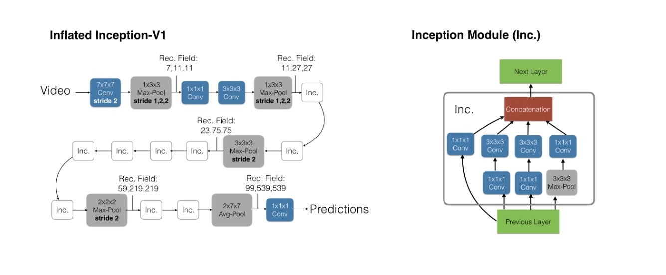
Figure 3. The Inflated Inception-V1 architecture (left) and its detailed inception submodule (right). The strides of convolution and pooling operators are 1 where not specified, and batch normalization layers, ReLu’s and the softmax at the end are not shown. The theoretical sizes of receptive field sizes for a few layers in the network are provided in the format “time,x,y” – the units are frames and pixels. The predictions are obtained convolutionally in time and averaged.
图 3. 膨胀后的 Inception-V1 结构(左)及其 Inception 子模块的细节(右)。未标明处,卷积和池化算子的步长为 1;批量归一化层、ReLU 以及最后的 softmax 未画出。网络中若干层的理论感受野大小以“时间, x, y”的格式给出,单位分别是帧和像素。预测在时间上以卷积方式得到,再取平均。
| Method | #Params | Training # Input Frames | Training Temporal Footprint | Testing # Input Frames | Testing Temporal Footprint |
|---|---|---|---|---|---|
| ConvNet+LSTM | 9M | 25 rgb | 5s | 50 rgb | 10s |
| 3D-ConvNet | 79M | 16 rgb | 0.64s | 240 rgb | 9.6s |
| Two-Stream | 12M | 1 rgb, 10 flow | 0.4s | 25 rgb, 250 flow | 10s |
| 3D-Fused | 39M | 5 rgb, 50 flow | 2s | 25 rgb, 250 flow | 10s |
| Two-Stream I3D | 25M | 64 rgb, 64 flow | 2.56s | 250 rgb, 250 flow | 10s |
| 方法 | 参数量 | 训练输入帧数 | 训练时间覆盖 | 测试输入帧数 | 测试时间覆盖 |
|---|---|---|---|---|---|
| ConvNet+LSTM | 9M | 25 rgb | 5s | 50 rgb | 10s |
| 3D-ConvNet | 79M | 16 rgb | 0.64s | 240 rgb | 9.6s |
| Two-Stream | 12M | 1 rgb, 10 flow | 0.4s | 25 rgb, 250 flow | 10s |
| 3D-Fused | 39M | 5 rgb, 50 flow | 2s | 25 rgb, 250 flow | 10s |
| Two-Stream I3D | 25M | 64 rgb, 64 flow | 2.56s | 250 rgb, 250 flow | 10s |
Table 1. Number of parameters and temporal input sizes of the models.
表 1. 各模型的参数量与时间输入规模。
We computed optical flow with a TV-L1 algorithm [35].
我们用 TV-L1 算法 [35] 计算光流。
3. The Kinetics Human Action Video Dataset
3. Kinetics 人类动作视频数据集
The Kinetics dataset is focused on human actions (rather than activities or events). The list of action classes covers: Person Actions (singular), e.g. drawing, drinking, laughing, punching; Person-Person Actions, e.g. hugging, kissing, shaking hands; and, Person-Object Actions, e.g. opening presents, mowing lawn, washing dishes. Some actions are fine grained and require temporal reasoning to distinguish, for example different types of swimming. Other actions require more emphasis on the object to distinguish, for example playing different types of wind instruments.
Kinetics 数据集关注的是人的动作(而不是活动或事件)。动作类别覆盖:单人动作,例如画画、喝水、笑、拳击;人人动作,例如拥抱、亲吻、握手;以及人与物体的动作,例如拆礼物、割草、洗碗。有些动作很细,需要时间推理才能区分,例如不同类型的游泳。另一些动作则更依赖所涉及的物体才能区分,例如演奏不同类型的管乐器。
The dataset has 400 human action classes, with 400 or more clips for each class, each from a unique video. The clips last around 10s, and there are no untrimmed videos. The test set consists of 100 clips for each class. A full description of the dataset and how it was built is given in [16].
该数据集有 400 个人类动作类别,每类有 400 条或更多片段,且每条来自不同的视频。片段长约 10 秒,没有未剪辑的长视频。测试集中每类有 100 条片段。关于数据集及其构建过程的完整说明见 [16]。
For most of the experiments in this paper we use a smaller dataset than the full Kinetics, called miniKinetics. This is an early version of the dataset having only 213 classes with a total of 120k clips across three splits, one for training with 150–1000 clips per class, one for validation with 25 clips per class and one for testing with 75 clips per class. MiniKinetics enabled faster experimentation, and was available before the full Kinetics dataset.
本文大多数实验使用的是比完整 Kinetics 更小的数据集,称为 miniKinetics。这是该数据集的一个早期版本,只有 213 类,三个划分合计约 12 万条片段:训练集每类 150–1000 条,验证集每类 25 条,测试集每类 75 条。miniKinetics 使实验可以更快进行,并且在完整 Kinetics 放出之前就可以使用。
4. Experimental Comparison of Architectures
4. 结构的实验比较
In this section we compare the performance of the five architectures described in section 2 whilst varying the dataset used for training and testing.
本节在变换训练和测试所用数据集的同时,比较第 2 节所述五种结构的性能。
| Architecture | UCF-101 RGB | UCF-101 Flow | UCF-101 RGB+Flow | HMDB-51 RGB | HMDB-51 Flow | HMDB-51 RGB+Flow | miniKinetics RGB | miniKinetics Flow | miniKinetics RGB+Flow |
|---|---|---|---|---|---|---|---|---|---|
| (a) LSTM | 81.0 | – | – | 36.0 | – | – | 69.9 | – | – |
| (b) 3D-ConvNet | 51.6 | – | – | 24.3 | – | – | 60.0 | – | – |
| (c) Two-Stream | 83.6 | 85.6 | 91.2 | 43.2 | 56.3 | 58.3 | 70.1 | 58.4 | 72.9 |
| (d) 3D-Fused | 83.2 | 85.8 | 89.3 | 49.2 | 55.5 | 56.8 | 71.4 | 61.0 | 74.0 |
| (e) Two-Stream I3D | 84.5 | 90.6 | 93.4 | 49.8 | 61.9 | 66.4 | 74.1 | 69.6 | 78.7 |
| 结构 | UCF-101 RGB | UCF-101 光流 | UCF-101 RGB+光流 | HMDB-51 RGB | HMDB-51 光流 | HMDB-51 RGB+光流 | miniKinetics RGB | miniKinetics 光流 | miniKinetics RGB+光流 |
|---|---|---|---|---|---|---|---|---|---|
| (a) LSTM | 81.0 | – | – | 36.0 | – | – | 69.9 | – | – |
| (b) 3D-ConvNet | 51.6 | – | – | 24.3 | – | – | 60.0 | – | – |
| (c) Two-Stream | 83.6 | 85.6 | 91.2 | 43.2 | 56.3 | 58.3 | 70.1 | 58.4 | 72.9 |
| (d) 3D-Fused | 83.2 | 85.8 | 89.3 | 49.2 | 55.5 | 56.8 | 71.4 | 61.0 | 74.0 |
| (e) Two-Stream I3D | 84.5 | 90.6 | 93.4 | 49.8 | 61.9 | 66.4 | 74.1 | 69.6 | 78.7 |
Table 2. Architecture comparison: (left) training and testing on split 1 of UCF-101; (middle) training and testing on split 1 of HMDB-51; (right) training and testing on miniKinetics. All models are based on Imagenet pre-trained Inception-v1, except 3D-ConvNet, a C3D-like [29] model which has a custom architecture and was trained here from scratch. Note that the Two-Stream architecture numbers on individual RGB and Flow streams can be interpreted as a simple baseline which applies a ConvNet independently on 25 uniformly sampled frames then averages the predictions.
表 2. 结构比较:(左)在 UCF-101 的 split 1 上训练和测试;(中)在 HMDB-51 的 split 1 上训练和测试;(右)在 miniKinetics 上训练和测试。除 3D-ConvNet 外,所有模型都以 ImageNet 预训练的 Inception-v1 为基础;3D-ConvNet 是类似 C3D [29] 的定制结构,这里从零开始训练。需要注意,双流结构在单独 RGB 和光流上的数字,也可以看成一种简单基线:对均匀采样的 25 帧各自施用 ConvNet,再把预测平均。
Table 2 shows the classification accuracy when training and testing on either UCF-101, HMDB-51 or miniKinetics. We test on the split 1 test sets of UCF-101 and HMDB-51 and on the held-out test set of miniKinetics. There are several noteworthy observations. First, our new I3D models do best in all datasets, with either RGB, flow, or RGB+flow modalities. This is interesting, given its very large number of parameters and that UCF-101 and HMDB-51 are so small, and shows that the benefits of ImageNet pre-training can extend to 3D ConvNets.
表 2 给出了在 UCF-101、HMDB-51 或 miniKinetics 上训练并测试时的分类准确率。我们在 UCF-101 和 HMDB-51 的 split 1 测试集上测试,并在 miniKinetics 的留出测试集上测试。有几点值得注意。第一,新的 I3D 模型在所有数据集上、无论是 RGB、光流还是 RGB+光流,都是最好的。考虑到它参数很多,而 UCF-101 和 HMDB-51 又很小,这一点很有意思,也说明 ImageNet 预训练的好处可以延伸到三维 ConvNet。
Second, the performance of all models is far lower on miniKinetics than on UCF-101, an indication of the different levels of difficulty of the two datasets. It is however higher than on HMDB-51; this may be in part due to lack of training data in HMDB-51 but also because this dataset was purposefully built to be hard: many clips have different actions in the exact same scene (e.g. “drawing sword” examples are taken from same videos as “sword” and “sword exercise”). Third, the ranking of the different architectures is mostly consistent. Fourth, the LSTM and 3D-ConvNet models are much more competitive on miniKinetics than on the smaller datasets; these models seem quite data-hungry.
第二,所有模型在 miniKinetics 上的表现都远低于 UCF-101,这反映了两份数据的难度不同。不过它仍高于 HMDB-51;这一方面可能是因为 HMDB-51 训练数据不足,另一方面也因为这份数据被有意做得很难:许多片段里,不同动作出现在完全相同的场景中(例如,“拔剑”的例子和“剑”“剑术练习”取自同一批视频)。第三,不同结构的排序大体一致。第四,LSTM 和 3D-ConvNet 在 miniKinetics 上要比在更小的数据集上有竞争力得多;这些模型看起来很吃数据。
Additionally, two-stream architectures exhibit superior performance on all datasets, but the relative value of RGB and flow differs significantly between miniKinetics and the other datasets. The contribution from flow alone, is slightly higher than that of RGB on UCF-101, much higher on HMDB-51, and substantially lower on miniKinetics. Visual inspection of the datasets suggests that Kinetics has much more camera motion which may make the job of the motion stream harder. The I3D model seems able to get more out of the flow stream than the other models, however, which can probably be explained by its much longer temporal receptive field (64 frames vs 10 during training) and more integrated temporal feature extraction machinery. While it seems plausible that the RGB stream has more discriminative information – we often struggled with our own eyes to discern actions from flow alone in Kinetics, and this was rarely the case from RGB – there may be opportunities for future research on integrating some form of motion stabilization into these architectures.
此外,双流结构在所有数据集上都更优,但 RGB 和光流的相对价值在 miniKinetics 与另外两份数据之间差别很大。仅看光流,它在 UCF-101 上略高于 RGB,在 HMDB-51 上高出很多,在 miniKinetics 上则明显更低。目视检查这些数据后可以猜想,Kinetics 里的相机运动更多,可能让运动流更难做。不过 I3D 似乎比其他模型更能利用光流,这大概是因为它的时间感受野长得多(训练时是 64 帧对 10 帧),而且时间特征提取也更一体。RGB 流含有更多判别信息看起来是合理的——我们常常即使用自己的眼睛,也很难只从 Kinetics 的光流里辨认出动作,而看 RGB 时很少遇到这种情况——因此,未来也许可以把某种运动稳定集成进这些结构。
5. Experimental Evaluation of Features
5. 特征的实验评估
In this section we investigate the generalizability of the networks trained on Kinetics. We consider two measures of this: first, we freeze the network weights and use the network to produce features for the (unseen) videos of the UCF-101/HMDB-51 datasets. We then train multi-way soft-max classifiers for the classes of UCF-101/HMDB-51 (using their training data), and evaluate on their test sets; Second, we fine-tune each network for the UCF-101/HMDB-51 classes (using the UCF-101/HMDB-51 training data), and again evaluate on the UCF-101/HMDB-51 test sets.
本节考察在 Kinetics 上训练的网络是否具有可泛化性。我们用两种方式衡量:第一,把网络权重冻结,用它给(未见过的)UCF-101/HMDB-51 视频提取特征,再在 UCF-101/HMDB-51 的训练数据上训练多类 softmax 分类器,并在其测试集上评估;第二,用 UCF-101/HMDB-51 的训练数据对每个网络做微调,再次在相应测试集上评估。
The results are given in table 3. The clear outcome is that all architectures benefit from pre-training on the additional video data of miniKinetics, but some benefit significantly more than the others – notably the I3D-ConvNet and 3D-ConvNet (although the latter starting from a much lower base). Training just the last layers of the models after pre-training in miniKinetics (Fixed) also leads to much better performance than directly training on UCF-101 and HMDB-51 for I3D models.
结果见表 3。清楚的结论是:所有结构都能从在 miniKinetics 的额外视频数据上预训练中获益,但有些结构获益明显更大——尤其是 I3D-ConvNet 和 3D-ConvNet(尽管后者起点低得多)。对 I3D 模型而言,在 miniKinetics 上预训练之后只训练最后几层(Fixed),也比直接在 UCF-101 和 HMDB-51 上训练好得多。
One explanation for the significant better transferability of features of I3D models is their high temporal resolution – they are trained on 64-frame video snippets at 25 frames per second and process all video frames at test time, which makes it possible for them to capture fine-grained temporal structure of actions. Stated differently, methods with sparser video inputs may benefit less from training on this large video dataset because, from their perspective, videos do not differ as much from the images in ImageNet. The difference over the C3D-like model can be explained by our I3D models being much deeper, while having much fewer parameters, by leveraging an ImageNet warm-start, by being trained on 4× longer videos, and by operating on 2× higher spatial resolution videos.
I3D 模型的特征可迁移性明显更好,一个解释是它们的时间分辨率高——它们在 25 帧/秒的 64 帧片段上训练,测试时处理全部视频帧,因而能够捕捉动作的细粒度时间结构。换句话说,输入更稀疏的方法从这份大规模视频数据中获益可能更少,因为在它们看来,这些视频与 ImageNet 中的图像差别并不那么大。与类似 C3D 的模型相比,我们的 I3D 要深得多,参数却少得多,又利用了 ImageNet 热启动,训练时用的视频长度是其 4 倍,并且在 2 倍空间分辨率的视频上运行。
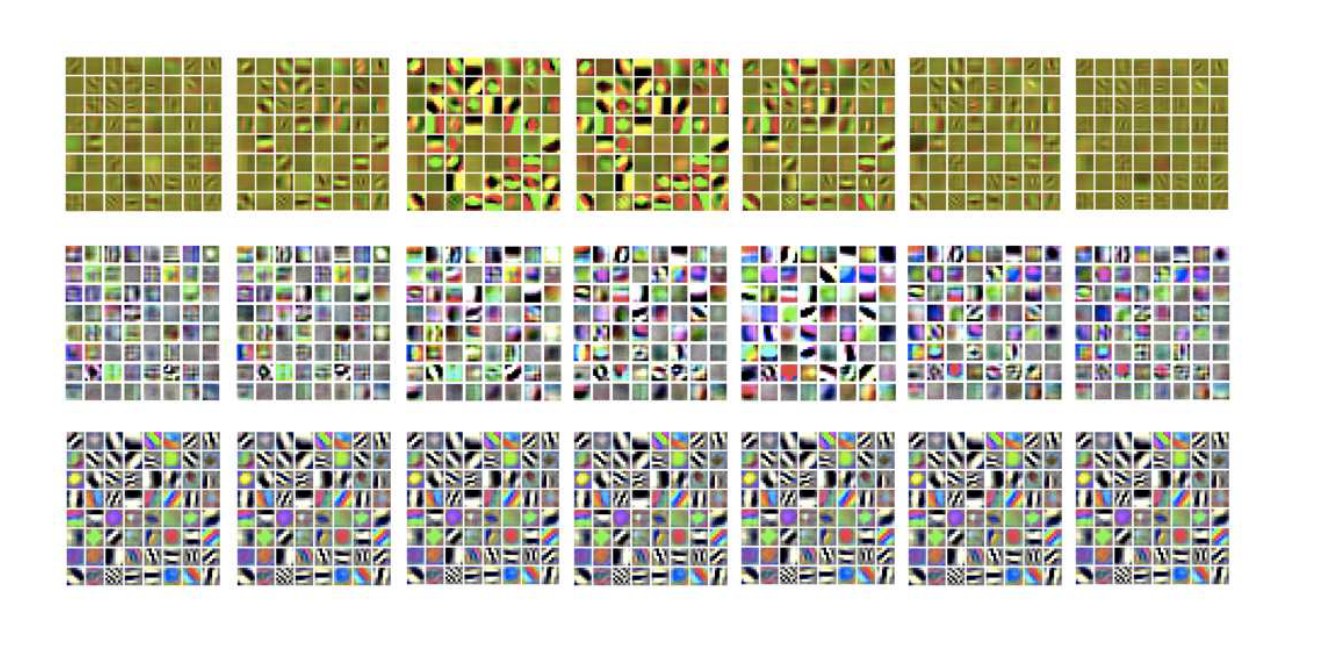
Figure 4. All 64 conv1 filters of each Inflated 3D ConvNet after training on Kinetics (the filter dimensions are 7 × 7 × 7, and the 7 time dimensions are shown left-to-right across the figure). The sequence on top shows the flow network filters, the one in the middle shows filters from the RGB I3D network, and the bottom row shows the original Inception-v1 filters. Note that the I3D filters possess rich temporal structure. Curiously the filters of the flow network are closer to the original Inception-v1 filters, while the filters in the RGB I3D network are no longer recognizable. Best seen on the computer, in colour and zoomed in.
图 4. 在 Kinetics 上训练后,每个膨胀三维 ConvNet 的全部 64 个 conv1 滤波核(滤波核尺寸为 7 × 7 × 7,7 个时间维在图中从左到右排列)。上排是光流网络的滤波核,中排是 RGB I3D 网络的滤波核,下排是原来的 Inception-v1 滤波核。可以看到 I3D 的滤波核具有丰富的时间结构。有意思的是,光流网络的滤波核更接近原来的 Inception-v1 滤波核,而 RGB I3D 中的滤波核已经不再容易辨认。最好在计算机上彩色显示并放大查看。
5.1. Comparison with the State-of-the-Art
5.1. 与当时最好结果的比较
We show a comparison of the performance of I3D models and previous state-of-the-art methods in table 4, on UCF-101 and HMDB-51. We include results when pre-training on miniKinetics and on the full Kinetics dataset. The conv1 filters of the trained models are shown in fig. 4.
表 4 给出了 I3D 模型与先前最好方法在 UCF-101 和 HMDB-51 上的比较。我们同时报告了在 miniKinetics 和完整 Kinetics 上预训练的结果。训练后模型的 conv1 滤波核见图 4。
Many methods get similar results, but the best performing method on these datasets is currently the one by Feichtenhofer and colleagues [7], which uses ResNet-50 models on RGB and optical flow streams, and gets 94.6% on UCF-101 and 70.3% on HMDB-51 when combined with the dense trajectories model [30]. We benchmarked our methods using the mean accuracy over the three standard train/test splits. Either of our RGB-I3D or RGB-Flow models alone, when pre-trained on Kinetics, outperforms all previous published performance by any model or model combinations. Our combined two-stream architecture widens the advantage over previous models considerably, bringing overall performance to 97.9 on UCF-101 and 80.2 on HMDB-51, which correspond to 57% and 33% misclassification reductions, respectively compared to the best previous model [7].
许多方法得到的结果相近,但当时在这两份数据上最好的,是 Feichtenhofer 及其同事的方法 [7]:它在 RGB 和光流上使用 ResNet-50,再与密集轨迹模型 [30] 结合,在 UCF-101 上达到 94.6%,在 HMDB-51 上达到 70.3%。我们用三个标准训练/测试划分上的平均准确率来评测自己的方法。只要在 Kinetics 上预训练,我们的 RGB-I3D 或光流 I3D 单独一路,就已经超过此前所有已发表的单一模型或模型组合。把两路合在一起后,优势进一步拉大,整体性能达到 UCF-101 上的 97.9 和 HMDB-51 上的 80.2,相对此前最好的模型 [7],分别把错误率降低了 57% 和 33%。
The difference between Kinetics pre-trained I3D models and prior 3D ConvNets (C3D) is even larger, although C3D is trained on more videos, 1M examples from Sports-1M plus an internal dataset, and even when ensembled and combined with IDT. This may be explainable by the better quality of Kinetics but also because of I3D simply being a better architecture.
在 Kinetics 上预训练的 I3D 与先前的三维 ConvNet(C3D)之间,差距甚至更大——尽管 C3D 训练用的视频更多,来自 Sports-1M 的 100 万个例子再加一份内部数据,而且即便把它做集成并与 IDT 结合也仍然如此。这也许可以解释为 Kinetics 质量更好,但也可以说只是因为 I3D 本身是更好的结构。
Another noteworthy effect is the improvement of the I3D RGB stream on HMDB-51 when going from miniKinetics to Kinetics pre-training, which suggests that 3D ConvNets may require large amounts of data in order to learn robust motion features. After Kinetics pre-training, the two streams obtain similar performance but are still complementary: averaging their predictions brings results from 74.6% to 80.2%.
另一个值得注意的现象是:I3D 的 RGB 流在 HMDB-51 上,从 miniKinetics 预训练改到 Kinetics 预训练后还有明显提升,这提示三维 ConvNet 可能需要大量数据才能学到稳健的运动特征。Kinetics 预训练之后,两路的表现已经接近,但仍互补:把它们的预测平均,结果从 74.6% 提高到 80.2%。
| Architecture | UCF-101 Original | UCF-101 Fixed | UCF-101 Full-FT | UCF-101 Δ | HMDB-51 Original | HMDB-51 Fixed | HMDB-51 Full-FT | HMDB-51 Δ |
|---|---|---|---|---|---|---|---|---|
| (a) LSTM | 81.0 | 81.6 | 82.1 | -6% | 36.0 | 46.6 | 46.4 | -10.6% |
| (b) 3D-ConvNet | 49.2 | 76.0 | 79.9 | -60.5% | 24.3 | 47.5 | 49.4 | -25.1% |
| (c) Two-Stream | 91.2 | 90.3 | 91.5 | -3.4% | 58.3 | 64.0 | 58.7 | -5.7% |
| (d) 3D-Fused | 89.3 | 88.5 | 90.1 | -7.5% | 56.8 | 59.0 | 61.4 | -4.6% |
| (e) Two-Stream I3D | 93.4 | 95.7 | 96.5 | -47.0% | 66.4 | 74.3 | 75.9 | -9.5% |
| 结构 | UCF-101 原始 | UCF-101 固定 | UCF-101 全微调 | UCF-101 Δ | HMDB-51 原始 | HMDB-51 固定 | HMDB-51 全微调 | HMDB-51 Δ |
|---|---|---|---|---|---|---|---|---|
| (a) LSTM | 81.0 | 81.6 | 82.1 | -6% | 36.0 | 46.6 | 46.4 | -10.6% |
| (b) 3D-ConvNet | 49.2 | 76.0 | 79.9 | -60.5% | 24.3 | 47.5 | 49.4 | -25.1% |
| (c) Two-Stream | 91.2 | 90.3 | 91.5 | -3.4% | 58.3 | 64.0 | 58.7 | -5.7% |
| (d) 3D-Fused | 89.3 | 88.5 | 90.1 | -7.5% | 56.8 | 59.0 | 61.4 | -4.6% |
| (e) Two-Stream I3D | 93.4 | 95.7 | 96.5 | -47.0% | 66.4 | 74.3 | 75.9 | -9.5% |
Table 3. Performance on the UCF-101 and HMDB-51 test sets (splits 1 of both) for architectures pre-trained on miniKinetics. All except 3D-ConvNet are based on Inception-v1 and start off pre-trained on ImageNet. Original: train on UCF-101 / HMDB-51; Fixed: features from miniKinetics, with the last layer trained on UCF-101 / HMDB-51; Full-FT: miniKinetics pre-training with end-to-end fine-tuning on UCF-101 / HMDB-51; ∆shows the difference in misclassification as percentage between Original and the best of Full-FT and Fixed.
表 3. 在 miniKinetics 上预训练的各结构,在 UCF-101 和 HMDB-51 测试集(均为 split 1)上的表现。除 3D-ConvNet 外,都以 Inception-v1 为基础,并先在 ImageNet 上预训练。Original:在 UCF-101 / HMDB-51 上训练;Fixed:使用来自 miniKinetics 的特征,只在 UCF-101 / HMDB-51 上训练最后一层;Full-FT:先在 miniKinetics 上预训练,再在 UCF-101 / HMDB-51 上做端到端微调;Δ 表示 Original 与 Full-FT、Fixed 中较好者之间,误分类率的百分比差。
| Model | UCF-101 | HMDB-51 |
|---|---|---|
| Two-Stream [25] | 88.0 | 59.4 |
| IDT [30] | 86.4 | 61.7 |
| Dynamic Image Networks + IDT [2] | 89.1 | 65.2 |
| TDD + IDT [31] | 91.5 | 65.9 |
| Two-Stream Fusion + IDT [8] | 93.5 | 69.2 |
| Temporal Segment Networks [32] | 94.2 | 69.4 |
| ST-ResNet + IDT [7] | 94.6 | 70.3 |
| Deep Networks [15], Sports 1M pre-training | 65.2 | – |
| C3D one network [29], Sports 1M pre-training | 82.3 | – |
| C3D ensemble [29], Sports 1M pre-training | 85.2 | – |
| C3D ensemble + IDT [29], Sports 1M pre-training | 90.1 | – |
| RGB-I3D, miniKinetics pre-training | 91.8 | 66.4 |
| RGB-I3D, Kinetics pre-training | 95.4 | 74.5 |
| Flow-I3D, miniKinetics pre-training | 94.7 | 72.4 |
| Flow-I3D, Kinetics pre-training | 95.4 | 74.6 |
| Two-Stream I3D, miniKinetics pre-training | 96.9 | 76.3 |
| Two-Stream I3D, Kinetics pre-training | 97.9 | 80.2 |
| 模型 | UCF-101 | HMDB-51 |
|---|---|---|
| Two-Stream [25] | 88.0 | 59.4 |
| IDT [30] | 86.4 | 61.7 |
| Dynamic Image Networks + IDT [2] | 89.1 | 65.2 |
| TDD + IDT [31] | 91.5 | 65.9 |
| Two-Stream Fusion + IDT [8] | 93.5 | 69.2 |
| Temporal Segment Networks [32] | 94.2 | 69.4 |
| ST-ResNet + IDT [7] | 94.6 | 70.3 |
| Deep Networks [15],Sports 1M 预训练 | 65.2 | – |
| C3D one network [29],Sports 1M 预训练 | 82.3 | – |
| C3D ensemble [29],Sports 1M 预训练 | 85.2 | – |
| C3D ensemble + IDT [29],Sports 1M 预训练 | 90.1 | – |
| RGB-I3D,miniKinetics 预训练 | 91.8 | 66.4 |
| RGB-I3D,Kinetics 预训练 | 95.4 | 74.5 |
| Flow-I3D,miniKinetics 预训练 | 94.7 | 72.4 |
| Flow-I3D,Kinetics 预训练 | 95.4 | 74.6 |
| Two-Stream I3D,miniKinetics 预训练 | 96.9 | 76.3 |
| Two-Stream I3D,Kinetics 预训练 | 97.9 | 80.2 |
Table 4. Comparison with state-of-the-art on the UCF-101 and HMDB-51 datasets, averaged over three splits. First set of rows contains results of models trained without labeled external data.
表 4. 在 UCF-101 和 HMDB-51 上与当时最好结果的比较,为三个划分上的平均。前一组是没有使用带标注外部数据训练的模型。
6. Discussion
6. 讨论
We return to the question posed in the introduction, “is there a benefit in transfer learning from videos?”. It is evident that there is a considerable benefit in pre-training on (the large video dataset) Kinetics, just as there has been such benefits in pre-training ConvNets on ImageNet for so many tasks. This demonstrates transfer learning from one dataset (Kinetics) to another dataset (UCF-101/HMDB-51) for a similar task (albeit for different action classes). However, it still remains to be seen if there is a benefit in using Kinetics pre-training for other video tasks such as semantic video segmentation, video object detection, or optical flow computation. We plan to make publicly available I3D models trained on the official Kinetics dataset’s release to facilitate research in this area.
我们回到引言中提出的问题:“从视频做迁移学习是否有好处?”答案是清楚的:在(大规模视频数据集)Kinetics 上预训练有可观的好处,正如在 ImageNet 上预训练 ConvNet 已经对许多任务带来的好处一样。这表明,从一个数据集(Kinetics)到另一个数据集(UCF-101/HMDB-51)、在相近任务上(尽管动作类别不同)可以做迁移学习。不过,Kinetics 预训练对视频语义分割、视频目标检测或光流计算等其他视频任务是否同样有益,当时仍有待观察。我们计划公开在正式发布的 Kinetics 上训练的 I3D 模型,以便利这一方向的研究。
Of course, we did not perform a comprehensive exploration of architectures – for example we have not employed action tubes [11, 17] or attention mechanisms [20] to focus in on the human actors. Recent works have proposed imaginative methods for determining the spatial and temporal extent (detection) of actors within the two-stream architectures, by incorporating linked object detections in time [22, 24]. The relationship between space and time is a mysterious one. Several very creative papers have recently gone out of the box in attempts to capture this relationship, for example by learning frame ranking functions for action classes and using these as a representation [9], by making analogies between actions and transformations [33], or by creating 2D visual snapshots of frame sequences [2] – this idea is related to the classic motion history work of [3]. It would be of great value to also include these models in our comparison but we could not, due to lack of time and space.
当然,我们并没有对结构做穷尽探索——例如,我们没有使用 action tubes [11, 17] 或注意力机制 [20] 来把焦点放在人物上。近期工作提出了一些富有想象力的方法,在双流结构里确定人物的空间与时间范围(检测),做法是把相互关联的物体检测在时间上连接起来 [22, 24]。空间与时间的关系仍然有些神秘。近来已有几篇很有创意的论文尝试跳出既有框框来刻画这一关系,例如学习用于动作类别的帧排序函数并以此作为表示 [9],在动作与变换之间做类比 [33],或把帧序列做成二维的视觉快照 [2]——这一想法与 [3] 的经典运动历史工作相关。若能把这些模型也纳入比较,会很有价值,但限于时间和篇幅,我们没能做到。
As future work, we plan to repeat all experiments using Kinetics instead of miniKinetics, with and without ImageNet pre-training, and explore inflating other state-of-the-art 2D ConvNets.
作为后续工作,我们计划用 Kinetics 代替 miniKinetics,在有无 ImageNet 预训练两种设定下重复全部实验,并探索把其他最先进的二维 ConvNet 也加以膨胀。
Acknowledgements:
致谢:
We would like to thank everyone on the Kinetics project and in particular Brian Zhang and Tim Green for help setting up the data for our experiments, and Karen Simonyan for comments, helpful clarifications and for sharing code.
我们感谢 Kinetics 项目组的所有成员,特别感谢 Brian Zhang 和 Tim Green 帮助为我们的实验准备数据,并感谢 Karen Simonyan 提出意见、做了有益的澄清,以及分享代码。
References
参考文献
[1] M. Abadi, A. Agarwal, P. Barham, E. Brevdo, Z. Chen, C. Citro, G. S. Corrado, A. Davis, J. Dean, M. Devin, et al. Tensorflow: Large-scale machine learning on heterogeneous distributed systems. arXiv preprint arXiv:1603.04467, 2016. 4
[2] H. Bilen, B. Fernando, E. Gavves, A. Vedaldi, and S. Gould. Dynamic image networks for action recognition. In IEEE International Conference on Computer Vision and Pattern Recognition CVPR, 2016. 8
[3] A. F. Bobick and J. W. Davis. The recognition of human movement using temporal templates. IEEE Transactions on pattern analysis and machine intelligence, 23(3):257–267, 2001. 8
[4] T. Cooijmans, N. Ballas, C. Laurent, and A. Courville. Recurrent batch normalization. arXiv preprint arXiv:1603.09025, 2016. 2
[5] J. Donahue, L. Anne Hendricks, S. Guadarrama, M. Rohrbach, S. Venugopalan, K. Saenko, and T. Darrell. Long-term recurrent convolutional networks for visual recognition and description. In Proceedings of the IEEE Conference on Computer Vision and Pattern Recognition, pages 2625–2634, 2015. 2
[6] A. Fathi and G. Mori. Action recognition by learning mid-level motion features. In Computer Vision and Pattern Recognition, 2008. CVPR 2008. IEEE Conference on, pages 1–8. IEEE, 2008. 2
[7] C. Feichtenhofer, A. Pinz, and R. P. Wildes. Spatiotemporal residual networks for video action recognition. arXiv preprint arXiv:1611.02155, 2016. 7, 8
[8] C. Feichtenhofer, A. Pinz, and A. Zisserman. Convolutional two-stream network fusion for video action recognition. In IEEE International Conference on Computer Vision and Pattern Recognition CVPR, 2016. 2, 3, 8
[9] B. Fernando, E. Gavves, J. M. Oramas, A. Ghodrati, and T. Tuytelaars. Modeling video evolution for action recognition. In Proceedings of the IEEE Conference on Computer Vision and Pattern Recognition, pages 5378–5387, 2015. 8
[10] R. Girshick, J. Donahue, T. Darrell, and J. Malik. Rich feature hierarchies for accurate object detection and semantic segmentation. In Proceedings of the IEEE conference on computer vision and pattern recognition, pages 580–587, 2014. 1
[11] G. Gkioxari and J. Malik. Finding action tubes. In Proceedings of the IEEE Conference on Computer Vision and Pattern Recognition, pages 759–768, 2015. 8
[12] K. He, X. Zhang, S. Ren, and J. Sun. Deep residual learning for image recognition. In Computer Vision and Pattern Recognition (CVPR), 2016 IEEE Conference on, 2016. 2
[13] S. Ioffe and C. Szegedy. Batch normalization: Accelerating deep network training by reducing internal covariate shift. arXiv preprint arXiv:1502.03167, 2015. 2, 4
[14] S. Ji, W. Xu, M. Yang, and K. Yu. 3d convolutional neural networks for human action recognition. IEEE transactions on pattern analysis and machine intelligence, 35(1):221–231, 2013. 2, 3
[15] A. Karpathy, G. Toderici, S. Shetty, T. Leung, R. Sukthankar, and L. Fei-Fei. Large-scale video classification with convolutional neural networks. In Proceedings of the IEEE conference on Computer Vision and Pattern Recognition, pages 1725–1732, 2014. 2, 3, 8
[16] W. Kay, J. Carreira, K. Simonyan, B. Zhang, C. Hillier, S. Vijayanarasimhan, F. Viola, T. Green, T. Back, P. Natsev, M. Suleyman, and A. Zisserman. The kinetics human action video dataset. arXiv preprint, 2017. 1, 5
[17] A. Kläser, M. Marszalek, C. Schmid, and A. Zisserman. Human focused action localization in video. In International Workshop on Sign, Gesture, Activity, ECCV 2010, 2010. 8
[18] H. Kuehne, H. Jhuang, E. Garrote, T. Poggio, and T. Serre. HMDB: a large video database for human motion recognition. In Proceedings of the International Conference on Computer Vision (ICCV), 2011. 1
[19] I. Laptev, M. Marszalek, C. Schmid, and B. Rozenfeld. Learning realistic human actions from movies. In Computer Vision and Pattern Recognition, 2008. CVPR 2008. IEEE Conference on, pages 1–8. IEEE, 2008. 2
[20] Z. Li, E. Gavves, M. Jain, and C. G. Snoek. VideoLSTM convolves, attends and flows for action recognition. arXiv preprint arXiv:1607.01794, 2016. 8
[21] J. C. Niebles, H. Wang, and L. Fei-Fei. Unsupervised learning of human action categories using spatial-temporal words. International journal of computer vision, 79(3):299–318, 2008. 2
[22] X. Peng and C. Schmid. Multi-region two-stream R-CNN for action detection. In European Conference on Computer Vision, pages 744–759. Springer, 2016. 8
[23] S. Ren, K. He, R. Girshick, and J. Sun. Faster r-cnn: Towards real-time object detection with region proposal networks. In Advances in neural information processing systems, pages 91–99, 2015. 1
[24] S. Saha, G. Singh, M. Sapienza, P. H. Torr, and F. Cuzzolin. Deep learning for detecting multiple space-time action tubes in videos. British Machine Vision Conference (BMVC) 2016, 2016. 8
[25] K. Simonyan and A. Zisserman. Two-stream convolutional networks for action recognition in videos. In Advances in Neural Information Processing Systems, pages 568–576, 2014. 2, 3, 8
[26] K. Simonyan and A. Zisserman. Very deep convolutional networks for large-scale image recognition. In ICLR, 2015. 2
[27] K. Soomro, A. R. Zamir, and M. Shah. UCF101: A dataset of 101 human actions classes from videos in the wild. arXiv preprint arXiv:1212.0402, 2012. 1
[28] G. W. Taylor, R. Fergus, Y. LeCun, and C. Bregler. Convolutional learning of spatio-temporal features. In European conference on computer vision, pages 140–153. Springer, 2010. 2, 3
[29] D. Tran, L. Bourdev, R. Fergus, L. Torresani, and M. Paluri. Learning spatiotemporal features with 3d convolutional networks. In 2015 IEEE International Conference on Computer Vision (ICCV), pages 4489–4497. IEEE, 2015. 2, 3, 6, 8
[30] H. Wang and C. Schmid. Action recognition with improved trajectories. In International Conference on Computer Vision, 2013. 2, 7, 8
[31] L. Wang, Y. Qiao, and X. Tang. Action recognition with trajectory-pooled deep-convolutional descriptors. In Proceedings of the IEEE Conference on Computer Vision and Pattern Recognition, pages 4305–4314, 2015. 8
[32] L. Wang, Y. Xiong, Z. Wang, Y. Qiao, D. Lin, X. Tang, and L. Van Gool. Temporal segment networks: towards good practices for deep action recognition. In European Conference on Computer Vision, 2016. 8
[33] X. Wang, A. Farhadi, and A. Gupta. Actions˜ transformations. arXiv preprint arXiv:1512.00795, 2015. 8
[34] J. Yue-Hei Ng, M. Hausknecht, S. Vijayanarasimhan, O. Vinyals, R. Monga, and G. Toderici. Beyond short snippets: Deep networks for video classification. In Proceedings of the IEEE Conference on Computer Vision and Pattern Recognition, pages 4694–4702, 2015. 2
[35] C. Zach, T. Pock, and H. Bischof. A duality based approach for realtime TV-L1 optical flow. Pattern Recognition, pages 214–223, 2007. 5