Human-level control through deep reinforcement learning

通过深度强化学习实现人类水平的控制

Volodymyr Mnih1*, Koray Kavukcuoglu1*, David Silver1*, Andrei A. Rusu1, Joel Veness1, Marc G. Bellemare1, Alex Graves1, Martin Riedmiller1, Andreas K. Fidjeland1, Georg Ostrovski1, Stig Petersen1, Charles Beattie1, Amir Sadik1, Ioannis Antonoglou1, Helen King1, Dharshan Kumaran1, Daan Wierstra1, Shane Legg1 & Demis Hassabis1

1Google DeepMind, 5 New Street Square, London EC4A 3TW, UK.

*These authors contributed equally to this work.

The theory of reinforcement learning provides a normative account1, deeply rooted in psychological2 and neuroscientific3 perspectives on animal behaviour, of how agents may optimize their control of an environment. To use reinforcement learning successfully in situations approaching real-world complexity, however, agents are confronted with a difficult task: they must derive efficient representations of the environment from high-dimensional sensory inputs, and use these to generalize past experience to new situations. Remarkably, humans and other animals seem to solve this problem through a harmonious combination of reinforcement learning and hierarchical sensory processing systems4,5, the former evidenced by a wealth of neural data revealing notable parallels between the phasic signals emitted by dopaminergic neurons and temporal difference reinforcement learning algorithms3. While reinforcement learning agents have achieved some successes in a variety of domains6–8, their applicability has previously been limited to domains in which useful features can be handcrafted, or to domains with fully observed, low-dimensional state spaces. Here we use recent advances in training deep neural networks9–11 to develop a novel artificial agent, termed a deep Q-network, that can learn successful policies directly from high-dimensional sensory inputs using end-to-end reinforcement learning. We tested this agent on the challenging domain of classic Atari 2600 games12. We demonstrate that the deep Q-network agent, receiving only the pixels and the game score as inputs, was able to surpass the performance of all previous algorithms and achieve a level comparable to that of a professional human games tester across a set of 49 games, using the same algorithm, network architecture and hyperparameters. This work bridges the divide between high-dimensional sensory inputs and actions, resulting in the first artificial agent that is capable of learning to excel at a diverse array of challenging tasks.

强化学习理论为智能体如何优化其对环境的控制提供了一种规范性说明1，其根基深植于关于动物行为的心理学2和神经科学3视角。然而，要在接近真实世界复杂程度的情境中成功使用强化学习，智能体面临一项困难任务：它们必须从高维感官输入中得到对环境的有效表示，并利用这些表示把过去的经验推广到新情境。值得注意的是，人和其他动物似乎通过强化学习与分层感官处理系统的协调结合解决了这一问题4,5；前者得到大量神经数据的支持，这些数据揭示了多巴胺能神经元发出的相位信号与时间差分强化学习算法之间显著的对应关系3。尽管强化学习智能体已在多种领域取得一些成功6–8，其适用范围此前一直局限于可以手工设计有用特征的领域，或状态完全可观察、维度较低的领域。在这里，我们利用训练深度神经网络的新近进展9–11，发展出一种称为深度 Q 网络的新型人工智能体，它能够用端到端强化学习直接从高维感官输入中学到成功的策略。我们在经典 Atari 2600 游戏这一具有挑战性的领域上测试了该智能体12。我们表明，这个深度 Q 网络智能体仅以像素和游戏得分为输入，就能够超过以往所有算法的表现，并在一组 49 款游戏上达到与职业人类游戏测试员相当的水平，而且使用的是同一套算法、网络结构和超参数。这项工作弥合了高维感官输入与动作之间的鸿沟，产生了第一个能够学会在多种具有挑战性的任务上表现出色的人工智能体。

We set out to create a single algorithm that would be able to develop a wide range of competencies on a varied range of challenging tasks—a central goal of general artificial intelligence13 that has eluded previous efforts8,14,15. To achieve this, we developed a novel agent, a deep Q-network (DQN), which is able to combine reinforcement learning with a class of artificial neural network16 known as deep neural networks. Notably, recent advances in deep neural networks9–11, in which several layers of nodes are used to build up progressively more abstract representations of the data, have made it possible for artificial neural networks to learn concepts such as object categories directly from raw sensory data. We use one particularly successful architecture, the deep convolutional network17, which uses hierarchical layers of tiled convolutional filters to mimic the effects of receptive fields—inspired by Hubel and Wiesel’s seminal work on feedforward processing in early visual cortex18—thereby exploiting the local spatial correlations present in images, and building in robustness to natural transformations such as changes of viewpoint or scale.

我们着手创造一种单一算法，使它能够在多种多样的挑战性任务上发展出广泛的能力——这是通用人工智能的一个核心目标13，却一直是以往努力未能达到的8,14,15。为此，我们发展了一种新型智能体，即深度 Q 网络（DQN），它能够把强化学习与一类称为深度神经网络的人工神经网络16结合起来。值得注意的是，深度神经网络的新近进展9–11用若干层节点逐步建立起对数据更抽象的表示，从而使人工神经网络能够直接从原始感官数据中学习诸如物体类别这样的概念。我们采用一种尤为成功的结构，即深度卷积网络17，它用分层排列、平铺的卷积滤波器来模拟感受野的效果——这一做法受到 Hubel 和 Wiesel 关于早期视皮层前馈加工的开创性研究的启发18——从而利用图像中存在的局部空间相关，并对视角或尺度变化这类自然变换建立起稳健性。

We consider tasks in which the agent interacts with an environment through a sequence of observations, actions and rewards. The goal of the agent is to select actions in a fashion that maximizes cumulative future reward. More formally, we use a deep convolutional neural network to approximate the optimal action-value function

我们考虑智能体通过观察、动作和奖励的序列与环境交互的任务。智能体的目标是以最大化累积未来奖励的方式选择动作。更形式地，我们用深度卷积神经网络来逼近最优动作价值函数

$$Q^*(s,a)=\max_{\pi}\mathbb{E}\!\left[r_t+\gamma r_{t+1}+\gamma^{2} r_{t+2}+\ldots\mid s_t=s,\,a_t=a,\,\pi\right]$$

which is the maximum sum of rewards $r_t$ discounted by $\gamma$ at each time-step $t$, achievable by a behaviour policy $\pi = P(a|s)$, after making an observation ($s$) and taking an action ($a$) (see Methods)19.

也就是在作出观察（$s$）并采取动作（$a$）之后，由行为策略 $\pi = P(a|s)$ 所能达到的、在每一时间步 $t$ 以 $\gamma$ 折现的奖励 $r_t$ 之和的最大值（见 Methods）19。

Reinforcement learning is known to be unstable or even to diverge when a nonlinear function approximator such as a neural network is used to represent the action-value (also known as Q) function20. This instability has several causes: the correlations present in the sequence of observations, the fact that small updates to $Q$ may significantly change the policy and therefore change the data distribution, and the correlations between the action-values ($Q$) and the target values $r+\gamma\max_{a'}Q(s',a')$. We address these instabilities with a novel variant of Q-learning, which uses two key ideas. First, we used a biologically inspired mechanism termed experience replay21–23 that randomizes over the data, thereby removing correlations in the observation sequence and smoothing over changes in the data distribution (see below for details). Second, we used an iterative update that adjusts the action-values ($Q$) towards target values that are only periodically updated, thereby reducing correlations with the target.

当用神经网络这类非线性函数逼近器来表示动作价值（也称 Q）函数时，强化学习已被认为不稳定，甚至会发散20。这种不稳定有几方面原因：观察序列中存在相关；对 $Q$ 的小更新可能显著改变策略，从而改变数据分布；以及动作价值（$Q$）与目标值 $r+\gamma\max_{a'}Q(s',a')$ 之间的相关。我们用一种新的 Q 学习变体来应对这些不稳定，其中用到两个关键想法。第一，我们采用一种受生物学启发、称为经验回放的机制21–23，在数据上做随机化，从而去掉观察序列中的相关，并平滑数据分布的变化（细节见下文）。第二，我们采用一种迭代更新，把动作价值（$Q$）向只定期更新的目标值调整，从而减弱与目标之间的相关。

While other stable methods exist for training neural networks in the reinforcement learning setting, such as neural fitted Q-iteration24, these methods involve the repeated training of networks de novo on hundreds of iterations. Consequently, these methods, unlike our algorithm, are too inefficient to be used successfully with large neural networks. We parameterize an approximate value function $Q(s,a;\theta_i)$ using the deep convolutional neural network shown in Fig. 1, in which $\theta_i$ are the parameters (that is, weights) of the Q-network at iteration $i$. To perform experience replay we store the agent’s experiences $e_t=(s_t,a_t,r_t,s_{t+1})$ at each time-step $t$ in a data set $D_t=\{e_1,\ldots,e_t\}$. During learning, we apply Q-learning updates, on samples (or minibatches) of experience $(s,a,r,s')\sim U(D)$, drawn uniformly at random from the pool of stored samples. The Q-learning update at iteration $i$ uses the following loss function:

虽然在强化学习设定下训练神经网络也存在其他稳定方法，例如神经拟合 Q 迭代24，但这些方法需要在数百次迭代中反复从头训练网络。因此，与我们的算法不同，这些方法效率太低，无法成功地用于大型神经网络。我们用图 1 所示的深度卷积神经网络来参数化近似价值函数 $Q(s,a;\theta_i)$，其中 $\theta_i$ 是第 $i$ 次迭代时 Q 网络的参数（即权重）。为了进行经验回放，我们在每一时间步 $t$ 把智能体的经验 $e_t=(s_t,a_t,r_t,s_{t+1})$ 存入数据集 $D_t=\{e_1,\ldots,e_t\}$。在学习过程中，我们从已存储样本池中均匀随机抽取经验样本（或小批量）$(s,a,r,s')\sim U(D)$，并在这些样本上施加 Q 学习更新。第 $i$ 次迭代的 Q 学习更新使用如下损失函数：

$$L_i(\theta_i)=\mathbb{E}_{(s,a,r,s')\sim U(D)}\Big[\big(r+\gamma\max_{a'}Q(s',a';\theta_i^-)-Q(s,a;\theta_i)\big)^2\Big]$$

in which $\gamma$ is the discount factor determining the agent’s horizon, $\theta_i$ are the parameters of the Q-network at iteration $i$ and $\theta_i^-$ are the network parameters used to compute the target at iteration $i$. The target network parameters $\theta_i^-$ are only updated with the Q-network parameters ($\theta_i$) every $C$ steps and are held fixed between individual updates (see Methods).

其中 $\gamma$ 是决定智能体视野的折现因子，$\theta_i$ 是第 $i$ 次迭代时 Q 网络的参数，$\theta_i^-$ 是在第 $i$ 次迭代中用于计算目标的网络参数。目标网络参数 $\theta_i^-$ 只每隔 $C$ 步才用 Q 网络参数（$\theta_i$）更新一次，并在各次更新之间保持固定（见 Methods）。

To evaluate our DQN agent, we took advantage of the Atari 2600 platform, which offers a diverse array of tasks ($n=49$) designed to be difficult and engaging for human players. We used the same network architecture, hyperparameter values (see Extended Data Table 1) and learning procedure throughout—taking high-dimensional data ($210\times 160$ colour video at 60 Hz) as input—to demonstrate that our approach robustly learns successful policies over a variety of games based solely on sensory inputs with only very minimal prior knowledge (that is, merely the input data were visual images, and the number of actions available in each game, but not their correspondences; see Methods). Notably, our method was able to train large neural networks using a reinforcement learning signal and stochastic gradient descent in a stable manner—illustrated by the temporal evolution of two indices of learning (the agent’s average score-per-episode and average predicted Q-values; see Fig. 2 and Supplementary Discussion for details).

为了评价我们的 DQN 智能体，我们利用了 Atari 2600 平台，它提供了一系列多种多样、对人类玩家而言既困难又有吸引力的任务（$n=49$）。我们自始至终使用同一套网络结构、超参数取值（见扩展数据表 1）和学习程序——以高维数据（60 Hz 的 $210\times 160$ 彩色视频）作为输入——以表明我们的方法能够仅依据感官输入、并只带有极少的先验知识，就在多种游戏上稳健地学到成功的策略（也就是说，事先只知道输入数据是视觉图像，以及每款游戏中可用的动作数目，而不知道它们的对应关系；见 Methods）。值得注意的是，我们的方法能够用强化学习信号和随机梯度下降，以稳定的方式训练大型神经网络——这一点由两项学习指标随时间的演化所说明（智能体的平均每局得分和平均预测 Q 值；见图 2 和 Supplementary Discussion）。

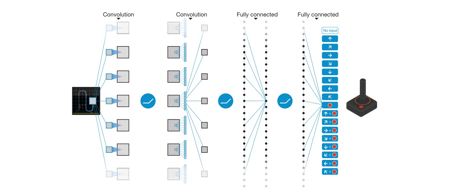
Figure 1 | Schematic illustration of the convolutional neural network. The details of the architecture are explained in the Methods. The input to the neural network consists of an $84\times 84\times 4$ image produced by the preprocessing map $\phi$, followed by three convolutional layers (note: snaking blue line symbolizes sliding of each filter across input image) and two fully connected layers with a single output for each valid action. Each hidden layer is followed by a rectifier nonlinearity (that is, $\max(0,x)$).

图 1｜卷积神经网络的示意。结构细节在 Methods 中说明。神经网络的输入是由预处理映射 $\phi$ 产生的 $84\times 84\times 4$ 图像，随后是三层卷积层（注：蛇形蓝线表示每个滤波器在输入图像上滑动）以及两层全连接层，每个合法动作对应一个输出。每个隐层之后都接一个整流非线性（即 $\max(0,x)$）。

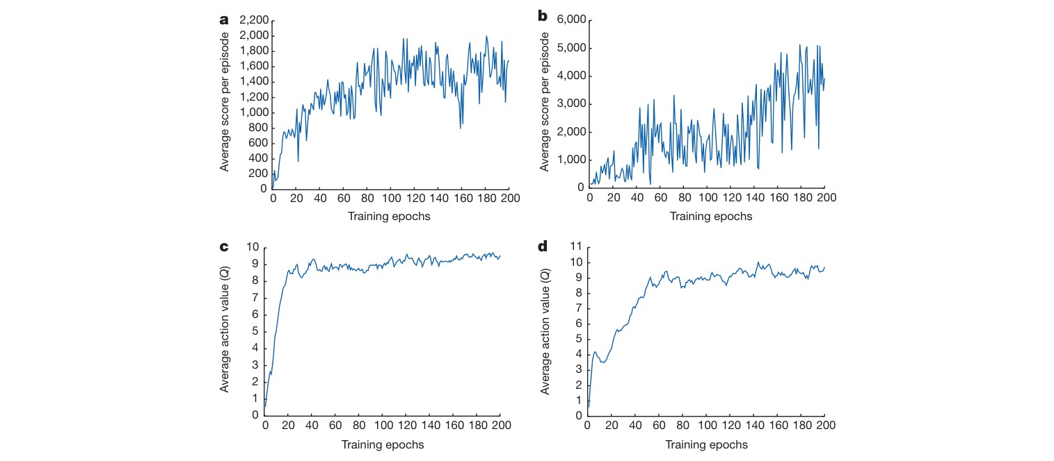
Figure 2 | Training curves tracking the agent’s average score and average predicted action-value. a, Each point is the average score achieved per episode after the agent is run with $\varepsilon$-greedy policy ($\varepsilon=0.05$) for 520 k frames on Space Invaders. b, Average score achieved per episode for Seaquest. c, Average predicted action-value on a held-out set of states on Space Invaders. d, Average predicted action-value on Seaquest. Each point on the curve is the average of the action-value $Q$ computed over the held-out set of states. Note that Q-values are scaled due to clipping of rewards (see Methods). See Supplementary Discussion for details.

图 2｜跟踪智能体平均得分和平均预测动作价值的训练曲线。a，智能体在 Space Invaders 上以 $\varepsilon$-greedy 策略（$\varepsilon=0.05$）运行 52 万帧后，每一点为平均每局得分。b，Seaquest 上平均每局得分。c，在 Space Invaders 一组留出状态上的平均预测动作价值。d，Seaquest 上的平均预测动作价值。曲线上每一点是在留出状态集上计算的动作价值 $Q$ 的平均值。注意，由于奖励被裁剪，Q 值经过了缩放（见 Methods）。细节见 Supplementary Discussion。

We compared DQN with the best performing methods from the reinforcement learning literature on the 49 games where results were available12,15. In addition to the learned agents, we also report scores for a professional human games tester playing under controlled conditions and a policy that selects actions uniformly at random (Extended Data Table 2 and Fig. 3, denoted by 100% (human) and 0% (random) on $y$ axis; see Methods). Our DQN method outperforms the best existing reinforcement learning methods on 43 of the games without incorporating any of the additional prior knowledge about Atari 2600 games used by other approaches (for example, refs 12, 15). Furthermore, our DQN agent performed at a level that was comparable to that of a professional human games tester across the set of 49 games, achieving more than 75% of the human score on more than half of the games (29 games; see Fig. 3, Supplementary Discussion and Extended Data Table 2). In additional simulations (see Supplementary Discussion and Extended Data Tables 3 and 4), we demonstrate the importance of the individual core components of the DQN agent—the replay memory, separate target Q-network and deep convolutional network architecture—by disabling them and demonstrating the detrimental effects on performance.

我们在已有结果可比较的 49 款游戏上，把 DQN 与强化学习文献中表现最好的方法做了比较12,15。除了所学智能体外，我们还报告了职业人类游戏测试员在受控条件下的得分，以及均匀随机选择动作的策略（扩展数据表 2 和图 3，$y$ 轴上分别记为 100%（人类）和 0%（随机）；见 Methods）。我们的 DQN 方法在 43 款游戏上超过了现有最好的强化学习方法，而且没有纳入其他方法所使用的关于 Atari 2600 游戏的额外先验知识（例如文献 12、15）。此外，我们的 DQN 智能体在这 49 款游戏上的表现与职业人类游戏测试员相当，在超过一半的游戏（29 款）上达到人类分数的 75% 以上（见图 3、Supplementary Discussion 和扩展数据表 2）。在补充模拟中（见 Supplementary Discussion 以及扩展数据表 3 和 4），我们通过关闭 DQN 智能体的各个核心组成部分——回放记忆、单独的目标 Q 网络和深度卷积网络结构——并展示对表现的不利影响，说明了这些部分的重要性。

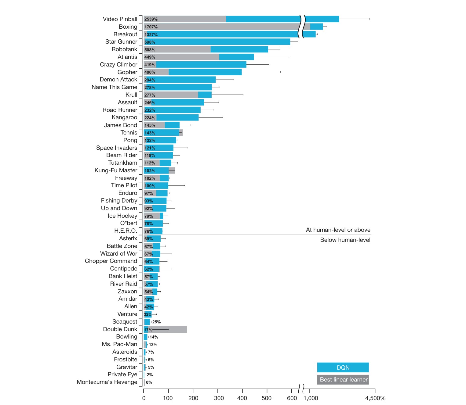
Figure 3 | Comparison of the DQN agent with the best reinforcement learning methods15 in the literature. The performance of DQN is normalized with respect to a professional human games tester (that is, 100% level) and random play (that is, 0% level). Note that the normalized performance of DQN, expressed as a percentage, is calculated as: $100\times(\text{DQN score}-\text{random play score})/(\text{human score}-\text{random play score})$. It can be seen that DQN outperforms competing methods (also see Extended Data Table 2) in almost all the games, and performs at a level that is broadly comparable with or superior to a professional human games tester (that is, operationalized as a level of 75% or above) in the majority of games. Audio output was disabled for both human players and agents. Error bars indicate s.d. across the 30 evaluation episodes, starting with different initial conditions.

图 3｜DQN 智能体与文献中最好的强化学习方法15的比较。DQN 的表现相对职业人类游戏测试员（即 100% 水平）和随机游戏（即 0% 水平）做了归一化。注意，以百分比表示的 DQN 归一化表现按 $100\times(\text{DQN 得分}-\text{随机游戏得分})/(\text{人类得分}-\text{随机游戏得分})$ 计算。可以看到，DQN 在几乎所有游戏上都超过了对比方法（亦见扩展数据表 2），并在大多数游戏上达到与职业人类游戏测试员大致相当或更好的水平（即达到 75% 或以上）。人类玩家和智能体的音频输出均被关闭。误差线表示从不同初始条件开始的 30 次评价对局的标准差。

We next examined the representations learned by DQN that underpinned the successful performance of the agent in the context of the game Space Invaders (see Supplementary Video 1 for a demonstration of the performance of DQN), by using a technique developed for the visualization of high-dimensional data called ‘t-SNE’25 (Fig. 4). As expected, the t-SNE algorithm tends to map the DQN representation of perceptually similar states to nearby points. Interestingly, we also found instances in which the t-SNE algorithm generated similar embeddings for DQN representations of states that are close in terms of expected reward but perceptually dissimilar (Fig. 4, bottom right, top left and middle), consistent with the notion that the network is able to learn representations that support adaptive behaviour from high-dimensional sensory inputs. Furthermore, we also show that the representations learned by DQN are able to generalize to data generated from policies other than its own—in simulations where we presented as input to the network game states experienced during human and agent play, recorded the representations of the last hidden layer, and visualized the embeddings generated by the t-SNE algorithm (Extended Data Fig. 1 and Supplementary Discussion). Extended Data Fig. 2 provides an additional illustration of how the representations learned by DQN allow it to accurately predict state and action values.

我们接下来考察了支撑智能体在游戏 Space Invaders 中成功表现的、由 DQN 学到的表示（DQN 表现的演示见 Supplementary Video 1），做法是使用一种为可视化高维数据而发展的技术，称为 “t-SNE”25（图 4）。正如所预期的，t-SNE 算法倾向于把感知上相似的状态的 DQN 表示映射到邻近的点。有意思的是，我们也发现了一些情形：对于在期望奖励上接近、但在感知上并不相似的状态，t-SNE 算法也为它们的 DQN 表示生成了相近的嵌入（图 4，右下、左上和中部），这与网络能够从高维感官输入中学到支持适应性行为的表示这一看法相一致。此外，我们还表明，DQN 学到的表示能够泛化到由其自身策略以外的策略所产生的数据——在模拟中，我们把人类和智能体游戏过程中经历的游戏状态作为输入呈现给网络，记录最后隐层的表示，并可视化由 t-SNE 算法生成的嵌入（扩展数据图 1 和 Supplementary Discussion）。扩展数据图 2 额外说明了 DQN 学到的表示如何使它能够准确预测状态价值和动作价值。

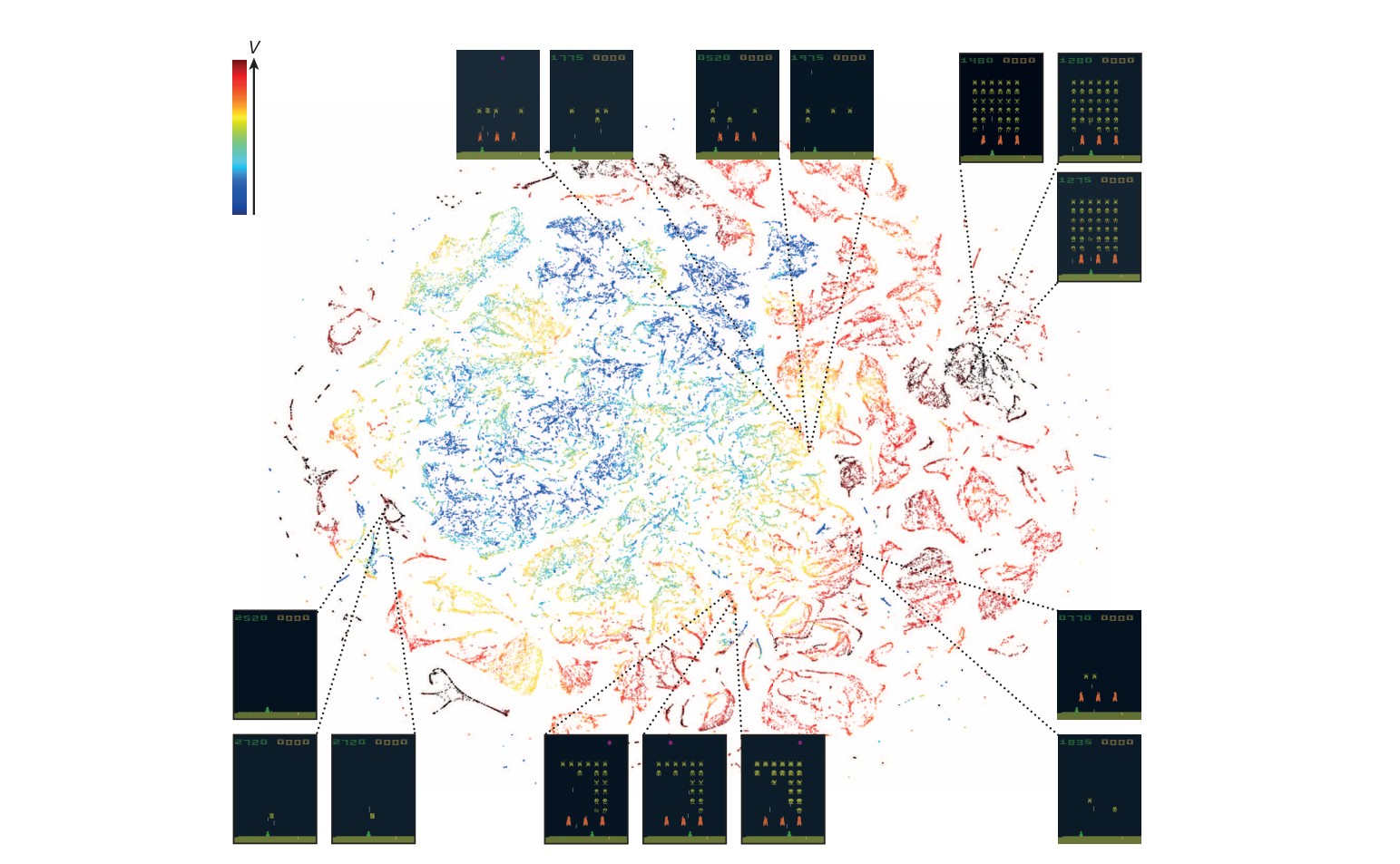
Figure 4 | Two-dimensional t-SNE embedding of the representations in the last hidden layer assigned by DQN to game states experienced while playing Space Invaders. The plot was generated by letting the DQN agent play for 2 h of real game time and running the t-SNE algorithm25 on the last hidden layer representations assigned by DQN to each experienced game state. The points are coloured according to the state values ($V$, maximum expected reward of a state) predicted by DQN for the corresponding game states (ranging from dark red (highest $V$) to dark blue (lowest $V$)). The screenshots corresponding to a selected number of points are shown. The DQN agent predicts high state values for both full (top right screenshots) and nearly complete screens (bottom left screenshots) because it has learned that completing a screen leads to a new screen full of enemy ships. Partially completed screens (bottom screenshots) are assigned lower state values because less immediate reward is available. The screens shown on the bottom right and top left and middle are less perceptually similar than the other examples but are still mapped to nearby representations and similar values because the orange bunkers do not carry great significance near the end of a level. With permission from Square Enix Limited.

图 4｜DQN 在玩 Space Invaders 时所经历的游戏状态上、赋予最后隐层表示的二维 t-SNE 嵌入。该图的生成方式是：让 DQN 智能体玩 2 小时实际游戏时间，再对 DQN 赋予每个所经历游戏状态的最后隐层表示运行 t-SNE 算法25。各点按 DQN 为相应游戏状态预测的状态价值（$V$，一个状态的最大期望奖励）着色（从深红（最高 $V$）到深蓝（最低 $V$））。图中给出了与若干选定点相对应的截图。DQN 智能体对满屏（右上截图）和接近完成的屏幕（左下截图）都预测出高状态价值，因为它已经学会：完成一屏会进入充满敌船的新一屏。部分完成的屏幕（下方截图）被赋予较低的状态价值，因为可立即获得的奖励更少。右下、左上和中部所示的画面在感知上不像其他例子那样相似，但仍被映射到邻近的表示和相近的价值，因为在一关接近结束时，橙色掩体已不再具有很大意义。经 Square Enix Limited 许可使用。

Indeed, in certain games DQN is able to discover a relatively long-term strategy (for example, Breakout: the agent learns the optimal strategy, which is to first dig a tunnel around the side of the wall allowing the ball to be sent around the back to destroy a large number of blocks; see Supplementary Video 2 for illustration of development of DQN’s performance over the course of training). Nevertheless, games demanding more temporally extended planning strategies still constitute a major challenge for all existing agents including DQN (for example, Montezuma’s Revenge).

的确，在某些游戏中，DQN 能够发现相对长期的策略（例如，在 Breakout 中：智能体学到了最优策略，即先在墙的侧面打出一条通道，让球从后方绕过去摧毁大量砖块；DQN 表现在训练过程中的发展见 Supplementary Video 2）。尽管如此，更需要在时间上延伸的规划策略的游戏，对包括 DQN 在内的所有现有智能体仍构成重大挑战（例如 Montezuma’s Revenge）。

In this work, we demonstrate that a single architecture can successfully learn control policies in a range of different environments with only very minimal prior knowledge, receiving only the pixels and the game score as inputs, and using the same algorithm, network architecture and hyperparameters on each game, privy only to the inputs a human player would have. In contrast to previous work24,26, our approach incorporates ‘end-to-end’ reinforcement learning that uses reward to continuously shape representations within the convolutional network towards salient features of the environment that facilitate value estimation. This principle draws on neurobiological evidence that reward signals during perceptual learning may influence the characteristics of representations within primate visual cortex27,28. Notably, the successful integration of reinforcement learning with deep network architectures was critically dependent on our incorporation of a replay algorithm21–23 involving the storage and representation of recently experienced transitions. Convergent evidence suggests that the hippocampus may support the physical realization of such a process in the mammalian brain, with the time-compressed reactivation of recently experienced trajectories during offline periods21,22 (for example, waking rest) providing a putative mechanism by which value functions may be efficiently updated through interactions with the basal ganglia22. In the future, it will be important to explore the potential use of biasing the content of experience replay towards salient events, a phenomenon that characterizes empirically observed hippocampal replay29, and relates to the notion of ‘prioritized sweeping’30 in reinforcement learning. Taken together, our work illustrates the power of harnessing state-of-the-art machine learning techniques with biologically inspired mechanisms to create agents that are capable of learning to master a diverse array of challenging tasks.

在这项工作中，我们表明，单一结构可以在多种不同环境中成功学习控制策略，而且只需要极少的先验知识：仅以像素和游戏得分作为输入，在每款游戏上使用同一套算法、网络结构和超参数，所能获知的也只是人类玩家会拥有的那些输入。与以往工作24,26相比，我们的方法纳入了“端到端”强化学习，用奖励持续把卷积网络内的表示塑造成有助于价值估计的、环境中显著的特征。这一原则借鉴了神经生物学证据，即知觉学习过程中的奖励信号可能影响灵长类视皮层中表示的特性27,28。值得注意的是，强化学习与深度网络结构的成功结合，关键取决于我们纳入了一种涉及存储和表示新近经历转移的回放算法21–23。汇聚的证据提示，海马可能支持这一过程在哺乳动物脑中的物理实现：在离线时段21,22（例如清醒休息）对新近经历轨迹的时间压缩再激活，提供了一种通过与基底神经节交互来高效更新价值函数的假定机制22。未来，探索把经验回放的内容偏向显著事件的潜在用法将十分重要，这一现象是经验上观察到的海马回放的特征29，也与强化学习中“优先扫描”的概念相关30。综合来看，我们的工作说明了把当时最先进的机器学习技术与受生物学启发的机制结合起来，以创造能够学会掌握多种挑战性任务的智能体，具有怎样的力量。

It is worth noting that the games in which DQN excels are extremely varied in their nature, from side-scrolling shooters (River Raid) to boxing games (Boxing) and three-dimensional car-racing games (Enduro).

值得指出的是，DQN 表现优异的那些游戏在性质上极为多样，既有横向卷轴射击（River Raid），也有拳击游戏（Boxing）和三维赛车游戏（Enduro）。

Online Content Methods, along with any additional Extended Data display items and Source Data, are available in the online version of the paper; references unique to these sections appear only in the online paper.

在线内容 Methods，以及任何额外的扩展数据展示项目和 Source Data，可在论文的在线版本中获取；仅出现在这些部分的参考文献只见于在线论文。

Received 10 July 2014; accepted 16 January 2015.

2014 年 7 月 10 日收到；2015 年 1 月 16 日接受。

METHODS

方法

Our experimental setup amounts to using the following minimal prior knowledge: that the input data consisted of visual images (motivating our use of a convolutional deep network), the game-specific score (with no modification), number of actions, although not their correspondences (for example, specification of the up ‘button’) and the life count.

我们的实验安排相当于只使用如下极少的先验知识：输入数据由视觉图像组成（这促使我们使用卷积深度网络），游戏特定的得分（不做修改），动作数目——但不知道它们的对应关系（例如，并不指定“上”键），以及生命计数。

Preprocessing. Working directly with raw Atari 2600 frames, which are $210\times 160$ pixel images with a 128-colour palette, can be demanding in terms of computation and memory requirements. We apply a basic preprocessing step aimed at reducing the input dimensionality and dealing with some artefacts of the Atari 2600 emulator. First, to encode a single frame we take the maximum value for each pixel colour value over the frame being encoded and the previous frame. This was necessary to remove flickering that is present in games where some objects appear only in even frames while other objects appear only in odd frames, an artefact caused by the limited number of sprites Atari 2600 can display at once. Second, we then extract the Y channel, also known as luminance, from the RGB frame and rescale it to $84\times 84$. The function $\phi$ from algorithm 1 described below applies this preprocessing to the $m$ most recent frames and stacks them to produce the input to the $Q$-function, in which $m=4$, although the algorithm is robust to different values of $m$ (for example, 3 or 5).

预处理。直接使用原始 Atari 2600 帧——它们是带 128 色调色板的 $210\times 160$ 像素图像——在计算和内存需求上可能很重。我们施加一个基本的预处理步骤，目的是降低输入维度，并处理 Atari 2600 模拟器的一些伪影。第一，为了编码单帧，我们在当前被编码的帧和上一帧上，对每个像素的颜色值取最大值。这是为了去除闪烁：在有些游戏中，一些物体只出现在偶数帧，另一些只出现在奇数帧，这一伪影来自 Atari 2600 一次能显示的精灵数量有限。第二，我们再从 RGB 帧中提取 Y 通道（即亮度），并把它缩放到 $84\times 84$。下文算法 1 中的函数 $\phi$ 把这一预处理施加到最近的 $m$ 帧上，并将它们叠在一起，作为 $Q$ 函数的输入，其中 $m=4$，不过算法对 $m$ 的不同取值（例如 3 或 5）是稳健的。

Code availability. The source code can be accessed at https://sites.google.com/a/deepmind.com/dqn for non-commercial uses only.

代码可用性。源代码可在 https://sites.google.com/a/deepmind.com/dqn 获取，仅供非商业使用。

Model architecture. There are several possible ways of parameterizing $Q$ using a neural network. Because $Q$ maps history–action pairs to scalar estimates of their $Q$-value, the history and the action have been used as inputs to the neural network by some previous approaches24,26. The main drawback of this type of architecture is that a separate forward pass is required to compute the $Q$-value of each action, resulting in a cost that scales linearly with the number of actions. We instead use an architecture in which there is a separate output unit for each possible action, and only the state representation is an input to the neural network. The outputs correspond to the predicted $Q$-values of the individual actions for the input state. The main advantage of this type of architecture is the ability to compute $Q$-values for all possible actions in a given state with only a single forward pass through the network.

模型结构。用神经网络参数化 $Q$ 有几种可能的方式。由于 $Q$ 把历史–动作对映射为对其 $Q$ 值的标量估计，以往一些方法把历史和动作都作为神经网络的输入24,26。这类结构的主要缺点是，计算每个动作的 $Q$ 值都需要单独一次前向传播，代价随动作数目线性增长。我们转而采用一种结构：每个可能的动作有一个单独的输出单元，神经网络的输入则只有状态表示。这些输出对应于输入状态下各个动作的预测 $Q$ 值。这类结构的主要优点是，只需通过网络做一次前向传播，就能计算给定状态下所有可能动作的 $Q$ 值。

The exact architecture, shown schematically in Fig. 1, is as follows. The input to the neural network consists of an $84\times 84\times 4$ image produced by the preprocessing map $\phi$. The first hidden layer convolves 32 filters of $8\times 8$ with stride 4 with the input image and applies a rectifier nonlinearity31,32. The second hidden layer convolves 64 filters of $4\times 4$ with stride 2, again followed by a rectifier nonlinearity. This is followed by a third convolutional layer that convolves 64 filters of $3\times 3$ with stride 1 followed by a rectifier. The final hidden layer is fully-connected and consists of 512 rectifier units. The output layer is a fully-connected linear layer with a single output for each valid action. The number of valid actions varied between 4 and 18 on the games we considered.

精确结构如图 1 所示，具体如下。神经网络的输入是由预处理映射 $\phi$ 产生的 $84\times 84\times 4$ 图像。第一个隐层用 32 个 $8\times 8$、步长为 4 的滤波器与输入图像做卷积，并施加整流非线性31,32。第二个隐层用 64 个 $4\times 4$、步长为 2 的滤波器做卷积，同样后接整流非线性。再后面是第三层卷积层，用 64 个 $3\times 3$、步长为 1 的滤波器做卷积，后接整流器。最后的隐层是全连接的，由 512 个整流单元组成。输出层是全连接线性层，每个合法动作对应一个输出。在我们所考虑的游戏中，合法动作数在 4 到 18 之间变化。

Training details. We performed experiments on 49 Atari 2600 games where results were available for all other comparable methods12,15. A different network was trained on each game: the same network architecture, learning algorithm and hyperparameter settings (see Extended Data Table 1) were used across all games, showing that our approach is robust enough to work on a variety of games while incorporating only minimal prior knowledge (see below). While we evaluated our agents on unmodified games, we made one change to the reward structure of the games during training only. As the scale of scores varies greatly from game to game, we clipped all positive rewards at 1 and all negative rewards at $-1$, leaving 0 rewards unchanged. Clipping the rewards in this manner limits the scale of the error derivatives and makes it easier to use the same learning rate across multiple games. At the same time, it could affect the performance of our agent since it cannot differentiate between rewards of different magnitude. For games where there is a life counter, the Atari 2600 emulator also sends the number of lives left in the game, which is then used to mark the end of an episode during training.

训练细节。我们在 49 款 Atari 2600 游戏上进行了实验，这些游戏对所有其他可比方法都已有结果12,15。每一款游戏训练一个不同的网络：在所有游戏上使用同一套网络结构、学习算法和超参数设置（见扩展数据表 1），这表明我们的方法足够稳健，能够在多种游戏上工作，同时只纳入极少的先验知识（见下文）。虽然我们在未修改的游戏上评价智能体，但在训练时对游戏的奖励结构做了一处改动。由于不同游戏的分数尺度差异很大，我们把所有正奖励裁成 1，所有负奖励裁成 $-1$，0 奖励保持不变。这样裁剪奖励可以限制误差导数的尺度，也更容易在多款游戏上使用相同的学习率。与此同时，这可能影响我们智能体的表现，因为它无法区分不同幅度的奖励。对于有生命计数的游戏，Atari 2600 模拟器还会发送游戏中剩余的生命数，训练时用它来标记一局的结束。

In these experiments, we used the RMSProp (see http://www.cs.toronto.edu/~tijmen/csc321/slides/lecture_slides_lec6.pdf) algorithm with minibatches of size 32. The behaviour policy during training was $\varepsilon$-greedy with $\varepsilon$ annealed linearly from 1.0 to 0.1 over the first million frames, and fixed at 0.1 thereafter. We trained for a total of 50 million frames (that is, around 38 days of game experience in total) and used a replay memory of 1 million most recent frames.

在这些实验中，我们使用 RMSProp 算法（见 http://www.cs.toronto.edu/~tijmen/csc321/slides/lecture_slides_lec6.pdf），小批量大小为 32。训练时的行为策略是 $\varepsilon$-greedy，$\varepsilon$ 在前一百万帧上从 1.0 线性退火到 0.1，此后固定为 0.1。我们一共训练了 5000 万帧（也就是大约共 38 天的游戏经验），并使用容量为最近 100 万帧的回放记忆。

Following previous approaches to playing Atari 2600 games, we also use a simple frame-skipping technique15. More precisely, the agent sees and selects actions on every $k$th frame instead of every frame, and its last action is repeated on skipped frames. Because running the emulator forward for one step requires much less computation than having the agent select an action, this technique allows the agent to play roughly $k$ times more games without significantly increasing the runtime. We use $k=4$ for all games.

沿用以往玩 Atari 2600 游戏的方法，我们也使用一种简单的跳帧技术15。更准确地说，智能体不是在每一帧、而是在每第 $k$ 帧上看到画面并选择动作，被跳过的帧则重复它上一次的动作。由于把模拟器向前运行一步所需的计算，远少于让智能体选择一个动作，这一技术使智能体大约可以多玩 $k$ 倍的游戏，而运行时间不会显著增加。所有游戏都取 $k=4$。

The values of all the hyperparameters and optimization parameters were selected by performing an informal search on the games Pong, Breakout, Seaquest, Space Invaders and Beam Rider. We did not perform a systematic grid search owing to the high computational cost. These parameters were then held fixed across all other games. The values and descriptions of all hyperparameters are provided in Extended Data Table 1.

所有超参数和优化参数的取值，是通过在 Pong、Breakout、Seaquest、Space Invaders 和 Beam Rider 这几款游戏上做非正式搜索选定的。由于计算代价很高，我们没有做系统的网格搜索。这些参数随后在所有其他游戏上保持固定。全部超参数的取值和说明见扩展数据表 1。

Evaluation procedure. The trained agents were evaluated by playing each game 30 times for up to 5 min each time with different initial random conditions (‘no-op’; see Extended Data Table 1) and an $\varepsilon$-greedy policy with $\varepsilon=0.05$. This procedure is adopted to minimize the possibility of overfitting during evaluation. The random agent served as a baseline comparison and chose a random action at 10 Hz which is every sixth frame, repeating its last action on intervening frames. 10 Hz is about the fastest that a human player can select the ‘fire’ button, and setting the random agent to this frequency avoids spurious baseline scores in a handful of the games. We did also assess the performance of a random agent that selected an action at 60 Hz (that is, every frame). This had a minimal effect: changing the normalized DQN performance by more than 5% in only six games (Boxing, Breakout, Crazy Climber, Demon Attack, Krull and Robotank), and in all these games DQN outperformed the expert human by a considerable margin.

评价程序。训练好的智能体通过在每款游戏上玩 30 次来评价，每次最多 5 分钟，并采用不同的随机初始条件（“no-op”；见扩展数据表 1）以及 $\varepsilon=0.05$ 的 $\varepsilon$-greedy 策略。采用这一程序是为了尽量减少评价时过拟合的可能。随机智能体作为基线比较，以 10 Hz（也就是每第六帧）选择一个随机动作，并在中间的帧上重复上一次动作。10 Hz 大约是人类玩家能够按下“开火”键的最快速度，把随机智能体设成这一频率，可以避免在少数游戏中出现虚假的基线分数。我们也评估了以 60 Hz（即每一帧）选择动作的随机智能体的表现。影响很小：归一化 DQN 表现的变化超过 5% 的只有六款游戏（Boxing、Breakout、Crazy Climber、Demon Attack、Krull 和 Robotank），而且在这些游戏中 DQN 都以相当大的幅度超过了专家人类。

The professional human tester used the same emulator engine as the agents, and played under controlled conditions. The human tester was not allowed to pause, save or reload games. As in the original Atari 2600 environment, the emulator was run at 60 Hz and the audio output was disabled: as such, the sensory input was equated between human player and agents. The human performance is the average reward achieved from around 20 episodes of each game lasting a maximum of 5 min each, following around 2 h of practice playing each game.

职业人类测试员与智能体使用同一套模拟器引擎，并在受控条件下游戏。人类测试员不得暂停、保存或重新载入游戏。与原来的 Atari 2600 环境一样，模拟器以 60 Hz 运行，音频输出被关闭：因此，人类玩家与智能体的感官输入是对齐的。人类表现是在每款游戏练习约 2 小时之后，对大约 20 局、每局最长 5 分钟所取得的平均奖励。

Algorithm. We consider tasks in which an agent interacts with an environment, in this case the Atari emulator, in a sequence of actions, observations and rewards. At each time-step the agent selects an action $a_t$ from the set of legal game actions, $A=\{1,\ldots,K\}$. The action is passed to the emulator and modifies its internal state and the game score. In general the environment may be stochastic. The emulator’s internal state is not observed by the agent; instead the agent observes an image $x_t\in\mathbb{R}^d$ from the emulator, which is a vector of pixel values representing the current screen. In addition it receives a reward $r_t$ representing the change in game score. Note that in general the game score may depend on the whole previous sequence of actions and observations; feedback about an action may only be received after many thousands of time-steps have elapsed.

算法。我们考虑智能体在动作、观察和奖励的序列中与环境（这里是 Atari 模拟器）交互的任务。在每一时间步，智能体从合法游戏动作集合 $A=\{1,\ldots,K\}$ 中选择一个动作 $a_t$。该动作被传给模拟器，并改变其内部状态和游戏得分。一般而言，环境可以是随机的。模拟器的内部状态不被智能体观察到；智能体看到的是来自模拟器的图像 $x_t\in\mathbb{R}^d$，它是表示当前屏幕的像素值向量。此外，它还收到表示游戏得分变化的奖励 $r_t$。需要注意，一般而言，游戏得分可能依赖于此前整个动作和观察序列；关于一个动作的反馈可能要在成千上万个时间步之后才会收到。

Because the agent only observes the current screen, the task is partially observed33 and many emulator states are perceptually aliased (that is, it is impossible to fully understand the current situation from only the current screen $x_t$). Therefore, sequences of actions and observations, $s_t=x_1,a_1,x_2,\ldots,a_{t-1},x_t$, are input to the algorithm, which then learns game strategies depending upon these sequences. All sequences in the emulator are assumed to terminate in a finite number of time-steps. This formalism gives rise to a large but finite Markov decision process (MDP) in which each sequence is a distinct state. As a result, we can apply standard reinforcement learning methods for MDPs, simply by using the complete sequence $s_t$ as the state representation at time $t$.

由于智能体只观察到当前屏幕，该任务是部分可观察的33，而且许多模拟器状态在感知上是混叠的（也就是说，仅从当前屏幕 $x_t$ 不可能完全理解当前情境）。因此，动作和观察的序列 $s_t=x_1,a_1,x_2,\ldots,a_{t-1},x_t$ 被输入算法，算法再根据这些序列学习游戏策略。假定模拟器中的所有序列都在有限个时间步内终止。这一形式化得到一个很大但有限的马尔可夫决策过程（MDP），其中每个序列是一个不同的状态。因此，我们可以把标准的 MDP 强化学习方法直接用在这里，只需把完整序列 $s_t$ 当作时刻 $t$ 的状态表示。

The goal of the agent is to interact with the emulator by selecting actions in a way that maximizes future rewards. We make the standard assumption that future rewards are discounted by a factor of $\gamma$ per time-step ($\gamma$ was set to 0.99 throughout), and define the future discounted return at time $t$ as $R_t=\sum_{t'=t}^{T}\gamma^{t'-t}r_{t'}$, in which $T$ is the time-step at which the game terminates. We define the optimal action-value function $Q^*(s,a)$ as the maximum expected return achievable by following any policy, after seeing some sequence $s$ and then taking some action $a$, $Q^*(s,a)=\max_{\pi}\mathbb{E}[R_t\mid s_t=s,a_t=a,\pi]$ in which $\pi$ is a policy mapping sequences to actions (or distributions over actions).

智能体的目标是通过以最大化未来奖励的方式选择动作，来与模拟器交互。我们做标准假定：未来奖励在每一时间步按因子 $\gamma$ 折现（全文取 $\gamma=0.99$），并把时刻 $t$ 的未来折现回报定义为 $R_t=\sum_{t'=t}^{T}\gamma^{t'-t}r_{t'}$，其中 $T$ 是游戏终止的时间步。我们把最优动作价值函数 $Q^*(s,a)$ 定义为：在看到某个序列 $s$ 并随后采取某个动作 $a$ 之后，遵循任一策略所能达到的最大期望回报，$Q^*(s,a)=\max_{\pi}\mathbb{E}[R_t\mid s_t=s,a_t=a,\pi]$，其中 $\pi$ 是把序列映射到动作（或动作上的分布）的策略。

The optimal action-value function obeys an important identity known as the Bellman equation. This is based on the following intuition: if the optimal value $Q^*(s',a')$ of the sequence $s'$ at the next time-step was known for all possible actions $a'$, then the optimal strategy is to select the action $a'$ maximizing the expected value of $r+\gamma Q^*(s',a')$.

最优动作价值函数满足一个重要恒等式，即贝尔曼方程。其直观是：如果下一时间步序列 $s'$ 对所有可能动作 $a'$ 的最优价值 $Q^*(s',a')$ 已知，那么最优策略就是选择使 $r+\gamma Q^*(s',a')$ 的期望值最大的动作 $a'$。

$$Q^*(s,a)=\mathbb{E}_{s'}\big[r+\gamma\max_{a'}Q^*(s',a')\mid s,a\big]$$

The basic idea behind many reinforcement learning algorithms is to estimate the action-value function by using the Bellman equation as an iterative update, $Q_{i+1}(s,a)=\mathbb{E}_{s'}[r+\gamma\max_{a'}Q_i(s',a')\mid s,a]$. Such value iteration algorithms converge to the optimal action-value function, $Q_i\to Q^*$ as $i\to\infty$. In practice, this basic approach is impractical, because the action-value function is estimated separately for each sequence, without any generalization. Instead, it is common to use a function approximator to estimate the action-value function, $Q(s,a;\theta)\approx Q^*(s,a)$. In the reinforcement learning community this is typically a linear function approximator, but sometimes a nonlinear function approximator is used instead, such as a neural network. We refer to a neural network function approximator with weights $\theta$ as a $Q$-network. A $Q$-network can be trained by adjusting the parameters $\theta_i$ at iteration $i$ to reduce the mean-squared error in the Bellman equation, where the optimal target values $r+\gamma\max_{a'}Q^*(s',a')$ are substituted with approximate target values $y=r+\gamma\max_{a'}Q(s',a';\theta_i^-)$, using parameters $\theta_i^-$ from some previous iteration. This leads to a sequence of loss functions $L_i(\theta_i)$ that changes at each iteration $i$,

许多强化学习算法背后的基本想法，是把贝尔曼方程当作迭代更新来估计动作价值函数，$Q_{i+1}(s,a)=\mathbb{E}_{s'}[r+\gamma\max_{a'}Q_i(s',a')\mid s,a]$。这类价值迭代算法收敛到最优动作价值函数，即当 $i\to\infty$ 时 $Q_i\to Q^*$。在实践中，这一基本做法并不可行，因为动作价值函数是对每个序列分别估计的，没有任何泛化。相反，通常用函数逼近器来估计动作价值函数，$Q(s,a;\theta)\approx Q^*(s,a)$。在强化学习社区中，这通常是线性函数逼近器，但有时也会改用非线性函数逼近器，例如神经网络。我们把权重为 $\theta$ 的神经网络函数逼近器称为 $Q$ 网络。$Q$ 网络可以通过在第 $i$ 次迭代调整参数 $\theta_i$、以减小贝尔曼方程中的均方误差来训练，其中最优目标值 $r+\gamma\max_{a'}Q^*(s',a')$ 被换成近似目标值 $y=r+\gamma\max_{a'}Q(s',a';\theta_i^-)$，使用的是此前某次迭代的参数 $\theta_i^-$。由此得到一组在每次迭代 $i$ 都会变化的损失函数 $L_i(\theta_i)$，

$$L_i(\theta_i)=\mathbb{E}_{s,a,r}\Big[\big(\mathbb{E}_{s'}[y\mid s,a]-Q(s,a;\theta_i)\big)^2\Big]=\mathbb{E}_{s,a,r,s'}\big[(y-Q(s,a;\theta_i))^2\big]+\mathbb{E}_{s,a,r}\big[\mathrm{Var}_{s'}[y]\big]$$

Note that the targets depend on the network weights; this is in contrast with the targets used for supervised learning, which are fixed before learning begins. At each stage of optimization, we hold the parameters from the previous iteration $\theta_{i-1}$ fixed when optimizing the $i$th loss function $L_i(\theta_i)$, resulting in a sequence of well-defined optimization problems. The final term is the variance of the targets, which does not depend on the parameters $\theta_i$ that we are currently optimizing, and may therefore be ignored. Differentiating the loss function with respect to the weights we arrive at the following gradient:

需要注意，目标依赖于网络权重；这与监督学习中使用的、在学习开始前就固定的目标不同。在优化的每一阶段，我们在优化第 $i$ 个损失函数 $L_i(\theta_i)$ 时保持前一次迭代的参数 $\theta_{i-1}$ 固定，从而得到一系列定义良好的优化问题。最后一项是目标的方差，它不依赖于我们当前正在优化的参数 $\theta_i$，因而可以忽略。把损失函数对权重求导，得到如下梯度：

$$\nabla_{\theta_i}L_i(\theta_i)=\mathbb{E}_{s,a,r,s'}\Big[\big(r+\gamma\max_{a'}Q(s',a';\theta_i^-)-Q(s,a;\theta_i)\big)\nabla_{\theta_i}Q(s,a;\theta_i)\Big]$$

Rather than computing the full expectations in the above gradient, it is often computationally expedient to optimize the loss function by stochastic gradient descent. The familiar Q-learning algorithm19 can be recovered in this framework by updating the weights after every time step, replacing the expectations using single samples, and setting $\theta_i^-=\theta_{i-1}$.

与其计算上述梯度中的完整期望，通常在计算上更便捷的做法是用随机梯度下降来优化损失函数。熟悉的 Q 学习算法19可以在这一框架中恢复出来：在每一时间步更新权重，用单一样本替换期望，并令 $\theta_i^-=\theta_{i-1}$。

Note that this algorithm is model-free: it solves the reinforcement learning task directly using samples from the emulator, without explicitly estimating the reward and transition dynamics $P(r,s'|s,a)$. It is also off-policy: it learns about the greedy policy $a=\mathrm{argmax}_{a'}Q(s,a';\theta)$, while following a behaviour distribution that ensures adequate exploration of the state space. In practice, the behaviour distribution is often selected by an $\varepsilon$-greedy policy that follows the greedy policy with probability $1-\varepsilon$ and selects a random action with probability $\varepsilon$.

需要注意，这一算法是无模型的：它直接用模拟器中的样本来解决强化学习任务，并不显式估计奖励和转移动力学 $P(r,s'|s,a)$。它也是离策略的：它学习的是贪心策略 $a=\mathrm{argmax}_{a'}Q(s,a';\theta)$，同时遵循一种确保对状态空间有充分探索的行为分布。在实践中，行为分布常常由 $\varepsilon$-greedy 策略来选择，即以概率 $1-\varepsilon$ 遵循贪心策略，以概率 $\varepsilon$ 选择随机动作。

Training algorithm for deep Q-networks. The full algorithm for training deep Q-networks is presented in Algorithm 1. The agent selects and executes actions according to an $\varepsilon$-greedy policy based on $Q$. Because using histories of arbitrary length as inputs to a neural network can be difficult, our $Q$-function instead works on a fixed length representation of histories produced by the function $\phi$ described above. The algorithm modifies standard online Q-learning in two ways to make it suitable for training large neural networks without diverging.

深度 Q 网络的训练算法。训练深度 Q 网络的完整算法见算法 1。智能体根据基于 $Q$ 的 $\varepsilon$-greedy 策略选择并执行动作。由于把任意长度的历史作为神经网络输入可能很困难，我们的 $Q$ 函数转而作用在由上述函数 $\phi$ 产生的、固定长度的历史表示上。该算法从两个方面修改了标准的在线 Q 学习，以使它适合在不发散的情况下训练大型神经网络。

Algorithm 1: deep Q-learning with experience replay.

Initialize replay memory $D$ to capacity $N$
Initialize action-value function $Q$ with random weights $\theta$
Initialize target action-value function $\hat{Q}$ with weights $\theta^-=\theta$
For episode $=1,M$ do
  Initialize sequence $s_1=\{x_1\}$ and preprocessed sequence $\phi_1=\phi(s_1)$
  For $t=1,T$ do
    With probability $\varepsilon$ select a random action $a_t$
    otherwise select $a_t=\mathrm{argmax}_a Q(\phi(s_t),a;\theta)$
    Execute action $a_t$ in emulator and observe reward $r_t$ and image $x_{t+1}$
    Set $s_{t+1}=s_t,a_t,x_{t+1}$ and preprocess $\phi_{t+1}=\phi(s_{t+1})$
    Store transition $(\phi_t,a_t,r_t,\phi_{t+1})$ in $D$
    Sample random minibatch of transitions $(\phi_j,a_j,r_j,\phi_{j+1})$ from $D$
    Set $y_j=r_j$ if episode terminates at step $j+1$
    Set $y_j=r_j+\gamma\max_{a'}\hat{Q}(\phi_{j+1},a';\theta^-)$ otherwise
    Perform a gradient descent step on $(y_j-Q(\phi_j,a_j;\theta))^2$ with respect to the network parameters $\theta$
    Every $C$ steps reset $\hat{Q}=Q$
  End For
End For

算法 1：带经验回放的深度 Q 学习。

Initialize replay memory $D$ to capacity $N$
Initialize action-value function $Q$ with random weights $\theta$
Initialize target action-value function $\hat{Q}$ with weights $\theta^-=\theta$
For episode $=1,M$ do
  Initialize sequence $s_1=\{x_1\}$ and preprocessed sequence $\phi_1=\phi(s_1)$
  For $t=1,T$ do
    With probability $\varepsilon$ select a random action $a_t$
    otherwise select $a_t=\mathrm{argmax}_a Q(\phi(s_t),a;\theta)$
    Execute action $a_t$ in emulator and observe reward $r_t$ and image $x_{t+1}$
    Set $s_{t+1}=s_t,a_t,x_{t+1}$ and preprocess $\phi_{t+1}=\phi(s_{t+1})$
    Store transition $(\phi_t,a_t,r_t,\phi_{t+1})$ in $D$
    Sample random minibatch of transitions $(\phi_j,a_j,r_j,\phi_{j+1})$ from $D$
    Set $y_j=r_j$ if episode terminates at step $j+1$
    Set $y_j=r_j+\gamma\max_{a'}\hat{Q}(\phi_{j+1},a';\theta^-)$ otherwise
    Perform a gradient descent step on $(y_j-Q(\phi_j,a_j;\theta))^2$ with respect to the network parameters $\theta$
    Every $C$ steps reset $\hat{Q}=Q$
  End For
End For

First, we use a technique known as experience replay23 in which we store the agent’s experiences at each time-step, $e_t=(s_t,a_t,r_t,s_{t+1})$, in a data set $D_t=\{e_1,\ldots,e_t\}$, pooled over many episodes (where the end of an episode occurs when a terminal state is reached) into a replay memory. During the inner loop of the algorithm, we apply Q-learning updates, or minibatch updates, to samples of experience, $(s,a,r,s')\sim U(D)$, drawn at random from the pool of stored samples. This approach has several advantages over standard online Q-learning. First, each step of experience is potentially used in many weight updates, which allows for greater data efficiency. Second, learning directly from consecutive samples is inefficient, owing to the strong correlations between the samples; randomizing the samples breaks these correlations and therefore reduces the variance of the updates. Third, when learning on-policy the current parameters determine the next data sample that the parameters are trained on. For example, if the maximizing action is to move left then the training samples will be dominated by samples from the left-hand side; if the maximizing action then switches to the right then the training distribution will also switch. It is easy to see how unwanted feedback loops may arise and the parameters could get stuck in a poor local minimum, or even diverge catastrophically20. By using experience replay, the behaviour distribution is averaged over many of its previous states, smoothing out learning and avoiding oscillations or divergence in the parameters. Note that when learning by experience replay, it is necessary to learn off-policy (because our current parameters are different to those used to generate the samples), which motivates the choice of Q-learning.

第一，我们使用一种称为经验回放的技术23：在每一时间步把智能体的经验 $e_t=(s_t,a_t,r_t,s_{t+1})$ 存入数据集 $D_t=\{e_1,\ldots,e_t\}$，并在许多对局上汇集（对局结束于到达终止状态时）到回放记忆中。在算法的内循环中，我们从已存储样本池中随机抽取经验样本 $(s,a,r,s')\sim U(D)$，并对它们施加 Q 学习更新或小批量更新。与标准在线 Q 学习相比，这一做法有几处优点。第一，每一步经验都有可能被用于多次权重更新，从而提高数据效率。第二，直接从连续样本学习效率不高，因为样本之间存在很强的相关；对样本做随机化会打破这些相关，从而降低更新的方差。第三，在策略学习时，当前参数决定了下一步用来训练这些参数的数据样本。例如，如果使价值最大的动作是向左移动，训练样本就会被左侧的样本所主导；如果最大动作随后转到右侧，训练分布也会跟着转。不难看出，不需要的反馈回路可能出现，参数可能卡在较差的局部极小，甚至灾难性地发散20。通过使用经验回放，行为分布会对其以往的许多状态取平均，从而平滑学习，并避免参数振荡或发散。需要注意，用经验回放学习时必须做离策略学习（因为我们当前的参数不同于产生这些样本时所用的参数），这也是选择 Q 学习的动机。

In practice, our algorithm only stores the last $N$ experience tuples in the replay memory, and samples uniformly at random from $D$ when performing updates. This approach is in some respects limited because the memory buffer does not differentiate important transitions and always overwrites with recent transitions owing to the finite memory size $N$. Similarly, the uniform sampling gives equal importance to all transitions in the replay memory. A more sophisticated sampling strategy might emphasize transitions from which we can learn the most, similar to prioritized sweeping30.

在实践中，我们的算法只在回放记忆中保存最近的 $N$ 个经验元组，并在做更新时从 $D$ 中均匀随机抽样。这一做法在某些方面是有局限的，因为记忆缓冲区并不区分重要的转移，并且由于有限的记忆容量 $N$，总是用新近的转移覆盖旧的。同样，均匀抽样对回放记忆中的所有转移给予同等重要性。更精细的抽样策略可能会强调那些我们能从中学到最多的转移，这类似于优先扫描30。

The second modification to online Q-learning aimed at further improving the stability of our method with neural networks is to use a separate network for generating the targets $y_j$ in the Q-learning update. More precisely, every $C$ updates we clone the network $Q$ to obtain a target network $\hat{Q}$ and use $\hat{Q}$ for generating the Q-learning targets $y_j$ for the following $C$ updates to $Q$. This modification makes the algorithm more stable compared to standard online Q-learning, where an update that increases $Q(s_t,a_t)$ often also increases $Q(s_{t+1},a)$ for all $a$ and hence also increases the target $y_j$, possibly leading to oscillations or divergence of the policy. Generating the targets using an older set of parameters adds a delay between the time an update to $Q$ is made and the time the update affects the targets $y_j$, making divergence or oscillations much more unlikely.

对在线 Q 学习的第二处修改，目的是进一步提高我们的方法在与神经网络结合时的稳定性，即在 Q 学习更新中用一个单独的网络来生成目标 $y_j$。更准确地说，每隔 $C$ 次更新，我们克隆网络 $Q$ 得到目标网络 $\hat{Q}$，并在随后对 $Q$ 的 $C$ 次更新中用 $\hat{Q}$ 生成 Q 学习目标 $y_j$。与标准在线 Q 学习相比，这一修改使算法更稳定：在标准在线 Q 学习中，一次使 $Q(s_t,a_t)$ 增大的更新，往往也会使所有 $a$ 的 $Q(s_{t+1},a)$ 增大，从而也增大目标 $y_j$，可能导致策略振荡或发散。用较旧的一组参数生成目标，在对 $Q$ 做出更新与该更新影响目标 $y_j$ 之间加入了延迟，从而使发散或振荡的可能性大大降低。

We also found it helpful to clip the error term from the update $r+\gamma\max_{a'}Q(s',a';\theta^-)-Q(s,a;\theta)$ to be between $-1$ and 1. Because the absolute value loss function $|x|$ has a derivative of $-1$ for all negative values of $x$ and a derivative of 1 for all positive values of $x$, clipping the squared error to be between $-1$ and 1 corresponds to using an absolute value loss function for errors outside of the $(-1,1)$ interval. This form of error clipping further improved the stability of the algorithm.

我们还发现，把更新中的误差项 $r+\gamma\max_{a'}Q(s',a';\theta^-)-Q(s,a;\theta)$ 裁剪到 $-1$ 和 1 之间是有帮助的。由于绝对值损失函数 $|x|$ 对所有负的 $x$ 导数为 $-1$，对所有正的 $x$ 导数为 1，把平方误差裁剪到 $-1$ 和 1 之间，对应于在 $(-1,1)$ 区间之外使用绝对值损失函数。这种形式的误差裁剪进一步提高了算法的稳定性。

References

参考文献

1. Sutton, R. & Barto, A. Reinforcement Learning: An Introduction (MIT Press, 1998).

2. Thorndike, E. L. Animal Intelligence: Experimental studies (Macmillan, 1911).

3. Schultz, W., Dayan, P. & Montague, P. R. A neural substrate of prediction and reward. Science 275, 1593–1599 (1997).

4. Serre, T., Wolf, L. & Poggio, T. Object recognition with features inspired by visual cortex. Proc. IEEE. Comput. Soc. Conf. Comput. Vis. Pattern. Recognit. 994–1000 (2005).

5. Fukushima, K. Neocognitron: A self-organizing neural network model for a mechanism of pattern recognition unaffected by shift in position. Biol. Cybern. 36, 193–202 (1980).

6. Tesauro, G. Temporal difference learning and TD-Gammon. Commun. ACM 38, 58–68 (1995).

7. Riedmiller, M., Gabel, T., Hafner, R. & Lange, S. Reinforcement learning for robot soccer. Auton. Robots 27, 55–73 (2009).

8. Diuk, C., Cohen, A. & Littman, M. L. An object-oriented representation for efficient reinforcement learning. Proc. Int. Conf. Mach. Learn. 240–247 (2008).

9. Bengio, Y. Learning deep architectures for AI. Foundations and Trends in Machine Learning 2, 1–127 (2009).

10. Krizhevsky, A., Sutskever, I. & Hinton, G. ImageNet classification with deep convolutional neural networks. Adv. Neural Inf. Process. Syst. 25, 1106–1114 (2012).

11. Hinton, G. E. & Salakhutdinov, R. R. Reducing the dimensionality of data with neural networks. Science 313, 504–507 (2006).

12. Bellemare, M. G., Naddaf, Y., Veness, J. & Bowling, M. The arcade learning environment: An evaluation platform for general agents. J. Artif. Intell. Res. 47, 253–279 (2013).

13. Legg, S. & Hutter, M. Universal Intelligence: a definition of machine intelligence. Minds Mach. 17, 391–444 (2007).

14. Genesereth, M., Love, N. & Pell, B. General game playing: overview of the AAAI competition. AI Mag. 26, 62–72 (2005).

15. Bellemare, M. G., Veness, J. & Bowling, M. Investigating contingency awareness using Atari 2600 games. Proc. Conf. AAAI. Artif. Intell. 864–871 (2012).

16. McClelland, J. L., Rumelhart, D. E. & Group, T. P. R. Parallel Distributed Processing: Explorations in the Microstructure of Cognition (MIT Press, 1986).

17. LeCun, Y., Bottou, L., Bengio, Y. & Haffner, P. Gradient-based learning applied to document recognition. Proc. IEEE 86, 2278–2324 (1998).

18. Hubel, D. H. & Wiesel, T. N. Shape and arrangement of columns in cat’s striate cortex. J. Physiol. 165, 559–568 (1963).

19. Watkins, C. J. & Dayan, P. Q-learning. Mach. Learn. 8, 279–292 (1992).

20. Tsitsiklis, J. & Roy, B. V. An analysis of temporal-difference learning with function approximation. IEEE Trans. Automat. Contr. 42, 674–690 (1997).

21. McClelland, J. L., McNaughton, B. L. & O’Reilly, R. C. Why there are complementary learning systems in the hippocampus and neocortex: insights from the successes and failures of connectionist models of learning and memory. Psychol. Rev. 102, 419–457 (1995).

22. O’Neill, J., Pleydell-Bouverie, B., Dupret, D. & Csicsvari, J. Play it again: reactivation of waking experience and memory. Trends Neurosci. 33, 220–229 (2010).

23. Lin, L.-J. Reinforcement learning for robots using neural networks. Technical Report, DTIC Document (1993).

24. Riedmiller, M. Neural fitted Q iteration - first experiences with a data efficient neural reinforcement learning method. Mach. Learn.: ECML, 3720, 317–328 (Springer, 2005).

25. Van der Maaten, L. J. P. & Hinton, G. E. Visualizing high-dimensional data using t-SNE. J. Mach. Learn. Res. 9, 2579–2605 (2008).

26. Lange, S. & Riedmiller, M. Deep auto-encoder neural networks in reinforcement learning. Proc. Int. Jt. Conf. Neural. Netw. 1–8 (2010).

27. Law, C.-T. & Gold, J. I. Reinforcement learning can account for associative and perceptual learning on a visual decision task. Nature Neurosci. 12, 655 (2009).

28. Sigala, N. & Logothetis, N. K. Visual categorization shapes feature selectivity in the primate temporal cortex. Nature 415, 318–320 (2002).

29. Bendor, D. & Wilson, M. A. Biasing the content of hippocampal replay during sleep. Nature Neurosci. 15, 1439–1444 (2012).

30. Moore, A. & Atkeson, C. Prioritized sweeping: reinforcement learning with less data and less real time. Mach. Learn. 13, 103–130 (1993).

31. Jarrett, K., Kavukcuoglu, K., Ranzato, M. A. & LeCun, Y. What is the best multi-stage architecture for object recognition? Proc. IEEE. Int. Conf. Comput. Vis. 2146–2153 (2009).

32. Nair, V. & Hinton, G. E. Rectified linear units improve restricted Boltzmann machines. Proc. Int. Conf. Mach. Learn. 807–814 (2010).

33. Kaelbling, L. P., Littman, M. L. & Cassandra, A. R. Planning and acting in partially observable stochastic domains. Artificial Intelligence 101, 99–134 (1994).

Supplementary Information is available in the online version of the paper.

补充信息可在论文的在线版本中获取。

Acknowledgements We thank G. Hinton, P. Dayan and M. Bowling for discussions, A. Cain and J. Keene for work on the visuals, K. Keller and P. Rogers for help with the visuals, G. Wayne for comments on an earlier version of the manuscript, and the rest of the DeepMind team for their support, ideas and encouragement.

致谢 我们感谢 G. Hinton、P. Dayan 和 M. Bowling 的讨论，感谢 A. Cain 和 J. Keene 在视觉呈现上的工作，感谢 K. Keller 和 P. Rogers 对视觉呈现的帮助，感谢 G. Wayne 对稿件较早版本的意见，并感谢 DeepMind 团队其余成员的支持、想法和鼓励。

Author Contributions V.M., K.K., D.S., J.V., M.G.B., M.R., A.G., D.W., S.L. and D.H. conceptualized the problem and the technical framework. V.M., K.K., A.A.R. and D.S. developed and tested the algorithms. J.V., S.P., C.B., A.A.R., M.G.B., I.A., A.K.F., G.O. and A.S. created the testing platform. K.K., H.K., S.L. and D.H. managed the project. K.K., D.K., D.H., V.M., D.S., A.G., A.A.R., J.V. and M.G.B. wrote the paper.

作者贡献 V.M.、K.K.、D.S.、J.V.、M.G.B.、M.R.、A.G.、D.W.、S.L. 和 D.H. 提出了问题和技术框架。V.M.、K.K.、A.A.R. 和 D.S. 发展并测试了算法。J.V.、S.P.、C.B.、A.A.R.、M.G.B.、I.A.、A.K.F.、G.O. 和 A.S. 创建了测试平台。K.K.、H.K.、S.L. 和 D.H. 管理了项目。K.K.、D.K.、D.H.、V.M.、D.S.、A.G.、A.A.R.、J.V. 和 M.G.B. 撰写了论文。

Author Information Reprints and permissions information is available at www.nature.com/reprints. The authors declare no competing financial interests. Readers are welcome to comment on the online version of the paper. Correspondence and requests for materials should be addressed to K.K. (korayk@google.com) or D.H. (demishassabis@google.com).

Extended Data

扩展数据

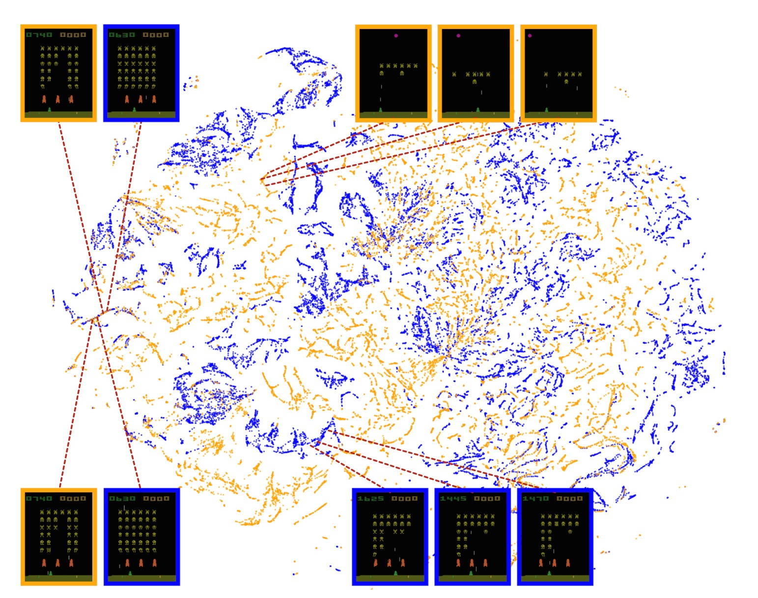
Extended Data Figure 1 | Two-dimensional t-SNE embedding of the representations in the last hidden layer assigned by DQN to game states experienced during a combination of human and agent play in Space Invaders. The plot was generated by running the t-SNE algorithm25 on the last hidden layer representation assigned by DQN to game states experienced during a combination of human (30 min) and agent (2 h) play. The fact that there is similar structure in the two-dimensional embeddings corresponding to the DQN representation of states experienced during human play (orange points) and DQN play (blue points) suggests that the representations learned by DQN do indeed generalize to data generated from policies other than its own. The presence in the t-SNE embedding of overlapping clusters of points corresponding to the network representation of states experienced during human and agent play shows that the DQN agent also follows sequences of states similar to those found in human play. Screenshots corresponding to selected states are shown (human: orange border; DQN: blue border).

扩展数据图 1｜DQN 对 Space Invaders 中人类与智能体混合游戏所经历的游戏状态赋予的最后隐层表示的二维 t-SNE 嵌入。该图是对 DQN 赋予在人类（30 分钟）和智能体（2 小时）混合游戏中所经历状态的最后隐层表示运行 t-SNE 算法25 得到的。对应于人类游戏所经历状态的 DQN 表示（橙色点）与 DQN 游戏（蓝色点）的二维嵌入具有相似结构，这一事实表明，DQN 学到的表示确实能够泛化到由其自身策略以外的策略所产生的数据。t-SNE 嵌入中出现与人类和智能体游戏中所经历状态的网络表示相对应的重叠点簇，说明 DQN 智能体也遵循与人类游戏中所见相似的状态序列。图中给出了与选定状态相对应的截图（人类：橙色边框；DQN：蓝色边框）。

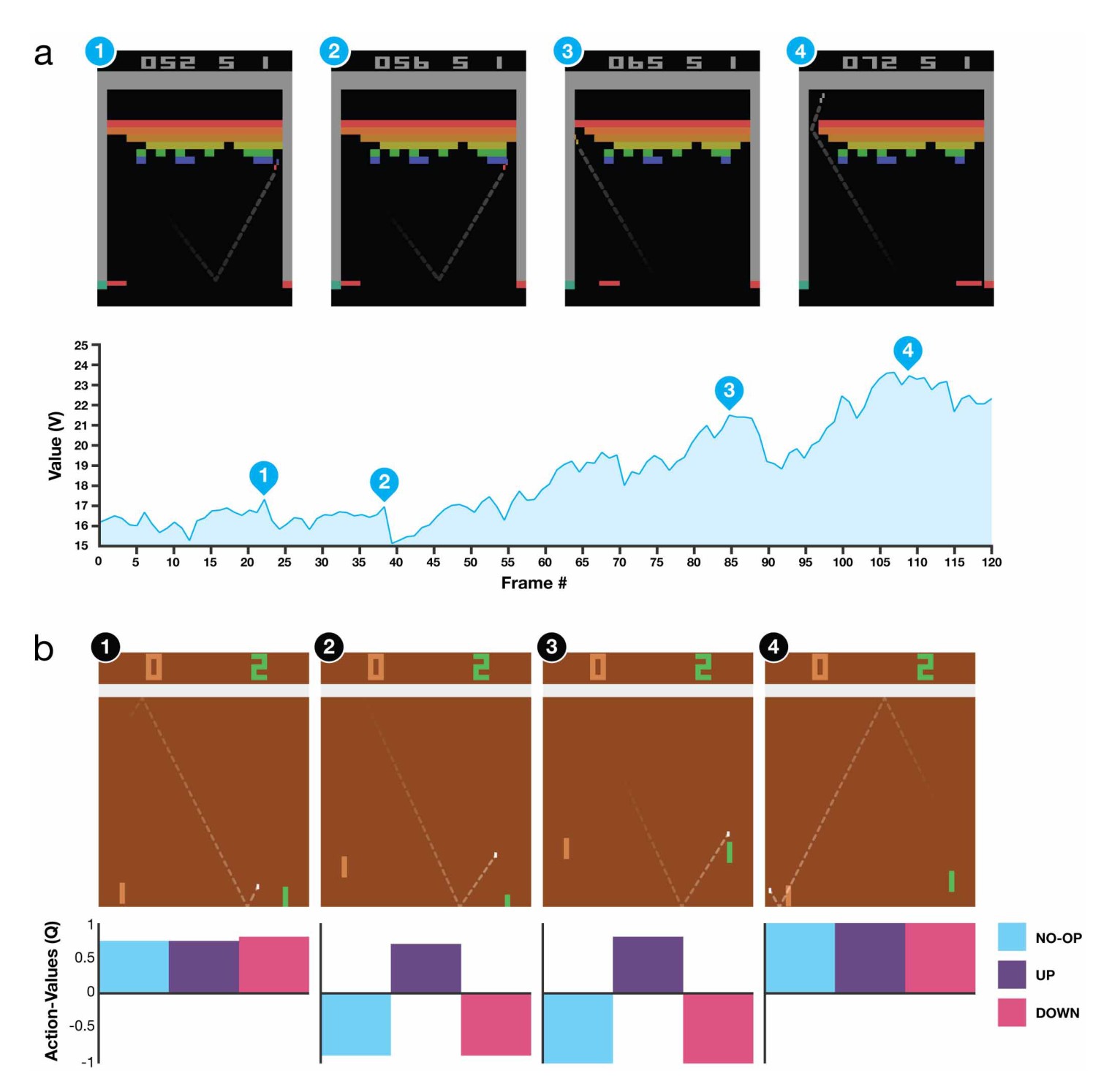
Extended Data Figure 2 | Visualization of learned value functions on two games, Breakout and Pong. a, A visualization of the learned value function on the game Breakout. At time points 1 and 2, the state value is predicted to be ∼17 and the agent is clearing the bricks at the lowest level. Each of the peaks in the value function curve corresponds to a reward obtained by clearing a brick. At time point 3, the agent is about to break through to the top level of bricks and the value increases to ∼21 in anticipation of breaking out and clearing a large set of bricks. At point 4, the value is above 23 and the agent has broken through. After this point, the ball will bounce at the upper part of the bricks clearing many of them by itself. b, A visualization of the learned action-value function on the game Pong. At time point 1, the ball is moving towards the paddle controlled by the agent on the right side of the screen and the values of all actions are around 0.7, reflecting the expected value of this state based on previous experience. At time point 2, the agent starts moving the paddle towards the ball and the value of the ‘up’ action stays high while the value of the ‘down’ action falls to −0.9. This reflects the fact that pressing ‘down’ would lead to the agent losing the ball and incurring a reward of −1. At time point 3, the agent hits the ball by pressing ‘up’ and the expected reward keeps increasing until time point 4, when the ball reaches the left edge of the screen and the value of all actions reflects that the agent is about to receive a reward of 1. Note, the dashed line shows the past trajectory of the ball purely for illustrative purposes (that is, not shown during the game). With permission from Atari Interactive, Inc.

扩展数据图 2｜两款游戏 Breakout 和 Pong 上学到的价值函数可视化。a，Breakout 上学到的价值函数可视化。在时间点 1 和 2，状态价值被预测为约 17，智能体正在清除最底层的砖块。价值函数曲线上的每个峰值，对应清除一块砖所获得的奖励。在时间点 3，智能体即将打通到最上层砖块，价值升到约 21，预期将打出通道并清除大量砖块。在点 4，价值高于 23，智能体已经打通。在此之后，球会在砖块上部弹跳，自行清除其中许多砖块。b，Pong 上学到的动作价值函数可视化。在时间点 1，球正朝屏幕右侧由智能体控制的球拍移动，所有动作的价值都在 0.7 左右，反映了基于以往经验的该状态期望价值。在时间点 2，智能体开始把球拍移向球，“上”动作的价值保持较高，而“下”动作的价值降到 −0.9。这反映出：按下“下”会导致智能体失球并得到 −1 的奖励。在时间点 3，智能体通过按下“上”击中了球，期望奖励持续增加，直到时间点 4，球到达屏幕左缘，所有动作的价值都反映出智能体即将得到 1 的奖励。注意，虚线仅出于示意目的给出球的过往轨迹（即游戏中并不显示）。经 Atari Interactive, Inc. 许可使用。

Hyperparameter	Value	Description
minibatch size	32	Number of training cases over which each stochastic gradient descent (SGD) update is computed.
replay memory size	1000000	SGD updates are sampled from this number of most recent frames.
agent history length	4	The number of most recent frames experienced by the agent that are given as input to the Q network.
target network update frequency	10000	The frequency (measured in the number of parameter updates) with which the target network is updated (this corresponds to the parameter $C$ from Algorithm 1).
discount factor	0.99	Discount factor gamma used in the Q-learning update.
action repeat	4	Repeat each action selected by the agent this many times. Using a value of 4 results in the agent seeing only every 4th input frame.
update frequency	4	The number of actions selected by the agent between successive SGD updates. Using a value of 4 results in the agent selecting 4 actions between each pair of successive updates.
learning rate	0.00025	The learning rate used by RMSProp.
gradient momentum	0.95	Gradient momentum used by RMSProp.
squared gradient momentum	0.95	Squared gradient (denominator) momentum used by RMSProp.
min squared gradient	0.01	Constant added to the squared gradient in the denominator of the RMSProp update.
initial exploration	1	Initial value of $\varepsilon$ in $\varepsilon$-greedy exploration.
final exploration	0.1	Final value of $\varepsilon$ in $\varepsilon$-greedy exploration.
final exploration frame	1000000	The number of frames over which the initial value of $\varepsilon$ is linearly annealed to its final value.
replay start size	50000	A uniform random policy is run for this number of frames before learning starts and the resulting experience is used to populate the replay memory.
no-op max	30	Maximum number of ‘do nothing’ actions to be performed by the agent at the start of an episode.

Extended Data Table 1 | List of hyperparameters and their values

The values of all the hyperparameters were selected by performing an informal search on the games Pong, Breakout, Seaquest, Space Invaders and Beam Rider. We did not perform a systematic grid search owing to the high computational cost, although it is conceivable that even better results could be obtained by systematically tuning the hyperparameter values.

超参数	取值	说明
小批量大小	32	每次随机梯度下降（SGD）更新所使用的训练样本数。
回放记忆大小	1000000	SGD 更新从这样多的最近帧中抽样。
智能体历史长度	4	作为 Q 网络输入、由智能体经历的最近帧数。
目标网络更新频率	10000	目标网络更新的频率（以参数更新次数计；这对应于算法 1 中的参数 $C$）。
折现因子	0.99	Q 学习更新中使用的折现因子 gamma。
动作重复	4	把智能体选定的每个动作重复这样多次。取值为 4 时，智能体只看到每第 4 个输入帧。
更新频率	4	相邻两次 SGD 更新之间智能体选择的动作数。取值为 4 时，智能体在每对相邻更新之间选择 4 个动作。
学习率	0.00025	RMSProp 使用的学习率。
梯度动量	0.95	RMSProp 使用的梯度动量。
平方梯度动量	0.95	RMSProp 使用的平方梯度（分母）动量。
最小平方梯度	0.01	加到 RMSProp 更新分母中平方梯度上的常数。
初始探索	1	$\varepsilon$-greedy 探索中 $\varepsilon$ 的初始值。
最终探索	0.1	$\varepsilon$-greedy 探索中 $\varepsilon$ 的最终值。
最终探索帧	1000000	把 $\varepsilon$ 的初始值线性退火到最终值所经过的帧数。
回放起始大小	50000	在学习开始前，用均匀随机策略运行这样多帧，并用由此得到的经验填充回放记忆。
最大空操作	30	智能体在一局开始时最多执行的“什么也不做”动作数。

扩展数据表 1｜超参数及其取值的列表

所有超参数的取值，是通过在 Pong、Breakout、Seaquest、Space Invaders 和 Beam Rider 这几款游戏上做非正式搜索选定的。由于计算代价很高，我们没有做系统的网格搜索，尽管可以设想，系统地调节超参数取值还可能得到更好的结果。

Game	Random Play	Best Linear Learner	Contingency (SARSA)	Human	DQN (± std)	Normalized DQN (% Human)
Alien	227.8	939.2	103.2	6875	3069 (±1093)	42.7%
Amidar	5.8	103.4	183.6	1676	739.5 (±3024)	43.9%
Assault	222.4	628	537	1496	3359(±775)	246.2%
Asterix	210	987.3	1332	8503	6012 (±1744)	70.0%
Asteroids	719.1	907.3	89	13157	1629 (±542)	7.3%
Atlantis	12850	62687	852.9	29028	85641(±17600)	449.9%
Bank Heist	14.2	190.8	67.4	734.4	429.7 (±650)	57.7%
Battle Zone	2360	15820	16.2	37800	26300 (±7725)	67.6%
Beam Rider	363.9	929.4	1743	5775	6846 (±1619)	119.8%
Bowling	23.1	43.9	36.4	154.8	42.4 (±88)	14.7%
Boxing	0.1	44	9.8	4.3	71.8 (±8.4)	1707.9%
Breakout	1.7	5.2	6.1	31.8	401.2 (±26.9)	1327.2%
Centipede	2091	8803	4647	11963	8309(±5237)	63.0%
Chopper Command	811	1582	16.9	9882	6687 (±2916)	64.8%
Crazy Climber	10781	23411	149.8	35411	114103 (±22797)	419.5%
Demon Attack	152.1	520.5	0	3401	9711 (±2406)	294.2%
Double Dunk	-18.6	-13.1	-16	-15.5	-18.1 (±2.6)	17.1%
Enduro	0	129.1	159.4	309.6	301.8 (±24.6)	97.5%
Fishing Derby	-91.7	-89.5	-85.1	5.5	-0.8 (±19.0)	93.5%
Freeway	0	19.1	19.7	29.6	30.3 (±0.7)	102.4%
Frostbite	65.2	216.9	180.9	4335	328.3 (±250.5)	6.2%
Gopher	257.6	1288	2368	2321	8520 (±3279)	400.4%
Gravitar	173	387.7	429	2672	306.7 (±223.9)	5.3%
H.E.R.O.	1027	6459	7295	25763	19950 (±158)	76.5%
Ice Hockey	-11.2	-9.5	-3.2	0.9	-1.6 (±2.5)	79.3%
James Bond	29	202.8	354.1	406.7	576.7 (±175.5)	145.0%
Kangaroo	52	1622	8.8	3035	6740 (±2959)	224.2%
Krull	1598	3372	3341	2395	3805 (±1033)	277.0%
Kung-Fu Master	258.5	19544	29151	22736	23270 (±5955)	102.4%
Montezuma's Revenge	0	10.7	259	4367	0 (±0)	0.0%
Ms. Pacman	307.3	1692	1227	15693	2311(±525)	13.0%
Name This Game	2292	2500	2247	4076	7257 (±547)	278.3%
Pong	-20.7	-19	-17.4	9.3	18.9 (±1.3)	132.0%
Private Eye	24.9	684.3	86	69571	1788(±5473)	2.5%
Q*Bert	163.9	613.5	960.3	13455	10596 (±3294)	78.5%
River Raid	1339	1904	2650	13513	8316 (±1049)	57.3%
Road Runner	11.5	67.7	89.1	7845	18257 (±4268)	232.9%
Robotank	2.2	28.7	12.4	11.9	51.6 (±4.7)	509.0%
Seaquest	68.4	664.8	675.5	20182	5286(±1310)	25.9%
Space Invaders	148	250.1	267.9	1652	1976 (±893)	121.5%
Star Gunner	664	1070	9.4	10250	57997 (±3152)	598.1%
Tennis	-23.8	-0.1	0	-8.9	-2.5 (±1.9)	143.2%
Time Pilot	3568	3741	24.9	5925	5947 (±1600)	100.9%
Tutankham	11.4	114.3	98.2	167.6	186.7 (±41.9)	112.2%
Up and Down	533.4	3533	2449	9082	8456 (±3162)	92.7%
Venture	0	66	0.6	1188	380.0 (±238.6)	32.0%
Video Pinball	16257	16871	19761	17298	42684 (±16287)	2539.4%
Wizard of Wor	563.5	1981	36.9	4757	3393 (±2019)	67.5%
Zaxxon	32.5	3365	21.4	9173	4977 (±1235)	54.1%

Extended Data Table 2 | Comparison of games scores obtained by DQN agents with methods from the literature12,15 and a professional human games tester

Best Linear Learner is the best result obtained by a linear function approximator on different types of hand designed features12. Contingency (SARSA) agent figures are the results obtained in ref. 15. Note the figures in the last column indicate the performance of DQN relative to the human games tester, expressed as a percentage, that is, $100\times(\text{DQN score}-\text{random play score})/(\text{human score}-\text{random play score})$.

游戏	随机游戏	最好的线性学习器	Contingency（SARSA）	人类	DQN（± 标准差）	Normalized DQN (% 人类)
Alien	227.8	939.2	103.2	6875	3069 (±1093)	42.7%
Amidar	5.8	103.4	183.6	1676	739.5 (±3024)	43.9%
Assault	222.4	628	537	1496	3359(±775)	246.2%
Asterix	210	987.3	1332	8503	6012 (±1744)	70.0%
Asteroids	719.1	907.3	89	13157	1629 (±542)	7.3%
Atlantis	12850	62687	852.9	29028	85641(±17600)	449.9%
Bank Heist	14.2	190.8	67.4	734.4	429.7 (±650)	57.7%
Battle Zone	2360	15820	16.2	37800	26300 (±7725)	67.6%
Beam Rider	363.9	929.4	1743	5775	6846 (±1619)	119.8%
Bowling	23.1	43.9	36.4	154.8	42.4 (±88)	14.7%
Boxing	0.1	44	9.8	4.3	71.8 (±8.4)	1707.9%
Breakout	1.7	5.2	6.1	31.8	401.2 (±26.9)	1327.2%
Centipede	2091	8803	4647	11963	8309(±5237)	63.0%
Chopper Command	811	1582	16.9	9882	6687 (±2916)	64.8%
Crazy Climber	10781	23411	149.8	35411	114103 (±22797)	419.5%
Demon Attack	152.1	520.5	0	3401	9711 (±2406)	294.2%
Double Dunk	-18.6	-13.1	-16	-15.5	-18.1 (±2.6)	17.1%
Enduro	0	129.1	159.4	309.6	301.8 (±24.6)	97.5%
Fishing Derby	-91.7	-89.5	-85.1	5.5	-0.8 (±19.0)	93.5%
Freeway	0	19.1	19.7	29.6	30.3 (±0.7)	102.4%
Frostbite	65.2	216.9	180.9	4335	328.3 (±250.5)	6.2%
Gopher	257.6	1288	2368	2321	8520 (±3279)	400.4%
Gravitar	173	387.7	429	2672	306.7 (±223.9)	5.3%
H.E.R.O.	1027	6459	7295	25763	19950 (±158)	76.5%
Ice Hockey	-11.2	-9.5	-3.2	0.9	-1.6 (±2.5)	79.3%
James Bond	29	202.8	354.1	406.7	576.7 (±175.5)	145.0%
Kangaroo	52	1622	8.8	3035	6740 (±2959)	224.2%
Krull	1598	3372	3341	2395	3805 (±1033)	277.0%
Kung-Fu Master	258.5	19544	29151	22736	23270 (±5955)	102.4%
Montezuma's Revenge	0	10.7	259	4367	0 (±0)	0.0%
Ms. Pacman	307.3	1692	1227	15693	2311(±525)	13.0%
Name This Game	2292	2500	2247	4076	7257 (±547)	278.3%
Pong	-20.7	-19	-17.4	9.3	18.9 (±1.3)	132.0%
Private Eye	24.9	684.3	86	69571	1788(±5473)	2.5%
Q*Bert	163.9	613.5	960.3	13455	10596 (±3294)	78.5%
River Raid	1339	1904	2650	13513	8316 (±1049)	57.3%
Road Runner	11.5	67.7	89.1	7845	18257 (±4268)	232.9%
Robotank	2.2	28.7	12.4	11.9	51.6 (±4.7)	509.0%
Seaquest	68.4	664.8	675.5	20182	5286(±1310)	25.9%
Space Invaders	148	250.1	267.9	1652	1976 (±893)	121.5%
Star Gunner	664	1070	9.4	10250	57997 (±3152)	598.1%
Tennis	-23.8	-0.1	0	-8.9	-2.5 (±1.9)	143.2%
Time Pilot	3568	3741	24.9	5925	5947 (±1600)	100.9%
Tutankham	11.4	114.3	98.2	167.6	186.7 (±41.9)	112.2%
Up and Down	533.4	3533	2449	9082	8456 (±3162)	92.7%
Venture	0	66	0.6	1188	380.0 (±238.6)	32.0%
Video Pinball	16257	16871	19761	17298	42684 (±16287)	2539.4%
Wizard of Wor	563.5	1981	36.9	4757	3393 (±2019)	67.5%
Zaxxon	32.5	3365	21.4	9173	4977 (±1235)	54.1%

扩展数据表 2｜DQN 智能体与文献中方法12,15以及职业人类游戏测试员的游戏得分比较

Best Linear Learner 是线性函数逼近器在不同类型手工设计特征上取得的最好结果12。Contingency（SARSA）智能体的数字是文献 15 中的结果。注意，最后一列的数字表示 DQN 相对人类游戏测试员的表现，以百分比给出，即 $100\times(\text{DQN 得分}-\text{随机游戏得分})/(\text{人类得分}-\text{随机游戏得分})$。

Game	With replay, with target Q	With replay, without target Q	Without replay, with target Q	Without replay, without target Q
Breakout	316.8	240.7	10.2	3.2
Enduro	1006.3	831.4	141.9	29.1
River Raid	7446.6	4102.8	2867.7	1453.0
Seaquest	2894.4	822.6	1003.0	275.8
Space Invaders	1088.9	826.3	373.2	302.0

Extended Data Table 3 | The effects of replay and separating the target Q-network

DQN agents were trained for 10 million frames using standard hyperparameters for all possible combinations of turning replay on or off, using or not using a separate target Q-network, and three different learning rates. Each agent was evaluated every 250,000 training frames for 135,000 validation frames and the highest average episode score is reported. Note that these evaluation episodes were not truncated at 5 min leading to higher scores on Enduro than the ones reported in Extended Data Table 2. Note also that the number of training frames was shorter (10 million frames) as compared to the main results presented in Extended Data Table 2 (50 million frames).

游戏	有回放，有目标 Q	有回放，无目标 Q	无回放，有目标 Q	无回放，无目标 Q
Breakout	316.8	240.7	10.2	3.2
Enduro	1006.3	831.4	141.9	29.1
River Raid	7446.6	4102.8	2867.7	1453.0
Seaquest	2894.4	822.6	1003.0	275.8
Space Invaders	1088.9	826.3	373.2	302.0

扩展数据表 3｜回放以及把目标 Q 网络分开的效果

DQN 智能体用标准超参数训练了 1000 万帧，覆盖打开或关闭回放、使用或不使用单独目标 Q 网络、以及三种不同学习率的所有可能组合。每个智能体每隔 25 万训练帧、用 13.5 万验证帧评价一次，并报告最高的平均对局得分。注意，这些评价对局没有在 5 分钟处截断，因而 Enduro 上的得分高于扩展数据表 2 中报告的结果。还需要注意，训练帧数更短（1000 万帧），而扩展数据表 2 中的主要结果是 5000 万帧。

Game	DQN	Linear
Breakout	316.8	3.00
Enduro	1006.3	62.0
River Raid	7446.6	2346.9
Seaquest	2894.4	656.9
Space Invaders	1088.9	301.3

Extended Data Table 4 | Comparison of DQN performance with linear function approximator

The performance of the DQN agent is compared with the performance of a linear function approximator on the 5 validation games (that is, where a single linear layer was used instead of the convolutional network, in combination with replay and separate target network). Agents were trained for 10 million frames using standard hyperparameters, and three different learning rates. Each agent was evaluated every 250,000 training frames for 135,000 validation frames and the highest average episode score is reported. Note that these evaluation episodes were not truncated at 5 min leading to higher scores on Enduro than the ones reported in Extended Data Table 2. Note also that the number of training frames was shorter (10 million frames) as compared to the main results presented in Extended Data Table 2 (50 million frames).

游戏	DQN	线性
Breakout	316.8	3.00
Enduro	1006.3	62.0
River Raid	7446.6	2346.9
Seaquest	2894.4	656.9
Space Invaders	1088.9	301.3

扩展数据表 4｜DQN 表现与线性函数逼近器的比较

在 5 款验证游戏上，把 DQN 智能体的表现与线性函数逼近器的表现进行比较（也就是用单层线性层替换卷积网络，并配合回放和单独的目标网络）。智能体用标准超参数以及三种不同学习率训练了 1000 万帧。每个智能体每隔 25 万训练帧、用 13.5 万验证帧评价一次，并报告最高的平均对局得分。注意，这些评价对局没有在 5 分钟处截断，因而 Enduro 上的得分高于扩展数据表 2 中报告的结果。还需要注意，训练帧数更短（1000 万帧），而扩展数据表 2 中的主要结果是 5000 万帧。