HuBERT: Self-Supervised Speech Representation Learning by Masked Prediction of Hidden Units

HuBERT：通过掩蔽预测隐单元的自监督语音表征学习

Wei-Ning Hsu    Benjamin Bolte    Yao-Hung Hubert Tsai    Kushal Lakhotia Affiliation:  Ruslan Salakhutdinov, Abdelrahman Mohamed

Abstract

摘要

Self-supervised approaches for speech representation learning are challenged by three unique problems: (1) there are multiple sound units in each input utterance, (2) there is no lexicon of input sound units during the pre-training phase, and (3) sound units have variable lengths with no explicit segmentation. To deal with these three problems, we propose the Hidden-Unit BERT (HuBERT) approach for self-supervised speech representation learning, which utilizes an offline clustering step to provide aligned target labels for a BERT-like prediction loss. A key ingredient of our approach is applying the prediction loss over the masked regions only, which forces the model to learn a combined acoustic and language model over the continuous inputs. HuBERT relies primarily on the consistency of the unsupervised clustering step rather than the intrinsic quality of the assigned cluster labels. Starting with a simple k-means teacher of 100 clusters, and using two iterations of clustering, the HuBERT model either matches or improves upon the state-of-the-art wav2vec 2.0 performance on the Librispeech (960h) and Libri-light (60,000h) benchmarks with 10min, 1h, 10h, 100h, and 960h fine-tuning subsets. Using a 1B parameter model, HuBERT shows up to 19% and 13% relative WER reduction on the more challenging dev-other and test-other evaluation subsets.[^1]

自监督语音表征学习面临三个独特问题：（1）每个输入话语中有多个声音单元；（2）预训练阶段没有输入声音单元词表；（3）声音单元长度可变且没有显式切分。为应对这三点，我们提出 Hidden-Unit BERT（HuBERT）：用离线聚类步骤提供与输入数据对齐的目标标签，用于类似 BERT 的预训练。关键之一是只对掩蔽区域施加预测损失，迫使模型在未掩蔽输入上学习良好高层表征，以便正确推断掩蔽处目标。直观上，该损失同时推动声学与长程时序结构的学习。HuBERT 依赖预测损失的一致性，而非聚类目标本身是否正确，因而聚类很差时仍可工作。经两次聚类迭代后，在 Librispeech（960h）与 Libri-light（6 万小时）上，对 10 分钟、1h、10h、100h、960h 微调子集达到或超过当时最好的 wav2vec 2.0。约 10 亿参数模型在更具挑战的 dev-other / test-other 上相对 WER 最高下降约 19% / 13%。[^1]

I Introduction

I 引言

Index Terms:

The north star for many research programs has been learning speech and audio representations through listening and interaction, similar to how babies learn their first language. High fidelity speech representation includes disentangled aspects of the spoken content along with non-lexical information of how it is delivered, e.g., speaker identity, emotion, hesitation, interruptions. Furthermore, reaching a complete situational understanding requires modeling structured noise interleaving and overlapping with the speech signal, e.g., laughter, coughing, lip-smacking, background vehicle engine, birds chirping, or food sizzling sounds.

索引词：

许多研究计划的北极星，是通过倾听与交互学习语音与音频表征，类似婴儿学习第一语言。高保真语音表征既包含已解耦的说话内容，也包含表达方式中的非词汇信息，例如说话人身份、情感、犹豫、打断。进一步，完整情境理解还需要对与语音交织、重叠的结构化噪声建模，例如笑声、咳嗽、咂嘴、背景引擎、鸟鸣或食物煎炸声。

The need for such high-fidelity representations drove research in self-supervised learning for speech and audio where the targets driving the learning process of a designed pretext task are drawn from the input signal itself. Examples of pretext tasks for self-supervised speech representation learning include distinguishing near-by features from temporally distant ones [1, 2, 3], next-step prediction of audio features [4], masked prediction of audio features given unmasked context [5, 6]. Besides, self-supervised learning methods do not rely on any linguistic resources during training, allowing them to learn universal representations since labels, annotations, and text-only material ignores rich information in the input signal.

对这类高保真表征的需求推动了语音与音频的自监督学习：设计的代理任务其目标来自输入信号本身。自监督语音表征学习的代理任务例子包括：把邻近特征与时间上远离的特征区分开 [1, 2, 3]、对音频特征做下一步预测 [4]、在给定未掩蔽上下文时对音频特征做掩蔽预测 [5, 6]。除表征学习本身外，这类方法也被证明能改善下游语音识别在低资源与跨领域设定下的表现。

Learning speech representations without reliance on large volumes of labeled data is crucial for industrial applications and products with ever-increasing coverage of new languages and domains. The time needed to collect large labeled datasets covering each of these scenarios is the real bottleneck in the current fast-moving AI industry, with time-to-market playing a critical role for product success. Building more inclusive applications covering spoken-only dialects and languages is another significant benefit of reducing dependence on linguistic resources. Given their non-standard orthographic rules, many of these languages and dialects have very little or no resources at all.

在不依赖大量有标注数据的情况下学习语音表征，对工业应用与产品至关重要——新产品要不断覆盖新语言与新领域。为每种场景收集大规模有标注数据所需的时间，才是当前快速迭代的 AI 产业真正瓶颈，上市时间对产品成败关键。构建更能包容仅口语方言与语言的应用，是另一重要动机：许多语言缺少书写系统或标准书写约定，大规模有标注采集几乎不可行。

Pseudo-labeling (PL), also known as self-training and belongs to the family of semi-supervised learning techniques, has been the dominant approach for utilizing unlabeled speech and audio with successful applications dating back to the mid-1990s [7, 8, 9, 10]. PL starts with some supervised data to train a ”teacher” model in one specific downstream task. Pseudo-labels are then generated for the unlabeled data using the teacher model. Next, a student model is trained using the combined supervised and teacher-labeled data either using the standard cross-entropy [9] loss or using a contrastive loss [11] to account for noise in teacher-generated labels. The pseudo-labeling process may be repeated multiple times to improve teacher label quality [12] iteratively.

伪标签（PL），也称自训练，属于半监督学习家族，一直是利用无标注语音与音频的主流做法，成功应用可追溯到 1990 年代中期 [7, 8, 9, 10]。PL 先用一些有监督数据在某一下游任务上训练“教师”模型，再用教师为无标注数据生成伪标签；随后用合并后的有监督与伪标签数据训练学生模型。该过程可迭代进行，学生变成下一轮教师。

Without discounting the immense success of pseudo-labeling techniques, self-supervised representations offer two unique advantages: (1) Pseudo-label methods force student models to merely mimic a teacher model, which is limited by its supervised data size and the provided annotation quality. On the other hand, self-supervised pretext tasks force the model to represent the entire input signal by compressing much more bits of information into the learned latent representation. (2) In pseudo-labeling, the supervised data of the teacher model forces the whole learning to be geared towards a single downstream task. On the contrary, self-supervised features show better generalization to a multitude of downstream applications.

在不贬低伪标签巨大成功的前提下，自监督表征有两点独特优势：（1）伪标签方法迫使学生只模仿教师，而教师受有监督数据规模与标注质量限制；自监督代理任务则迫使模型表征整个输入信号，把更多比特信息压进学到的潜表征。（2）伪标签绑定某一下游任务与标签空间；自监督预训练得到的表征可迁移到多种下游任务，包括语音识别、说话人、情感等。

There have been impressive successes for self-supervised learning in Computer Vision (CV) [13, 14, 15] and Natural Language Processing (NLP) [16, 17, 18] applications. Learning representations of discrete input sequences, such as in Natural Language Processing (NLP) applications, uses either masked prediction [19, 20] or auto-regressive generation [21, 18] of input sequences with partial obfuscation. For continuous inputs, such as in Computer Vision (CV) applications, representations are often learned through instance classification, in which each image and its augmentations are treated as a single output class to be pulled together [14, 15] or contrasted against other negative samples [22].

计算机视觉（CV）[13, 14, 15] 与自然语言处理（NLP）[16, 17, 18] 中的自监督学习已有显著成功。对离散输入序列（如 NLP），常用掩蔽预测 [19, 20] 或对部分混淆输入的自回归生成 [21, 18]。对连续输入（如 CV），表征常通过对抗或对比目标学习，使增强视图在嵌入空间中靠近 [13, 14, 15]。

Speech signals differ from text and images in that they are continuous-valued sequences. Self-supervised learning for the speech recognition domain faces unique challenges from those in CV and NLP. Firstly, the presence of multiple sounds in each input utterance breaks the instance classification assumption used in many CV pre-training approaches. Secondly, during pre-training, there is no prior lexicon of discrete sound units available, as in NLP applications in which words or word pieces are used, hindering the use of predictive losses. Lastly, the boundaries between sound units are not known, which complicates masked prediction pre-training.

语音信号与文本、图像不同，它是连续取值的序列。语音识别领域的自监督学习面临有别于 CV 与 NLP 的挑战。首先，每个输入话语中存在多个声音，打破了许多 CV 预训练所用的实例分类假设。其次，预训练时没有可用的离散声音单元先验词表——不像 NLP 中词或词片事先已知。再次，声音单元长度可变且没有显式切分。

In this paper, we introduce Hidden unit BERT (HuBERT) that benefits from an offline clustering step to generate noisy labels for a BERT-like per-training. Concretely, a BERT model consumes masked continuous speech features to predict pre-determined cluster assignments. The predictive loss is only applied over the masked regions, forcing the model to learn good high-level representations of unmasked inputs to infer the targets of masked ones correctly. Intuitively, the HuBERT model is forced to learn both acoustic and language models from continuous inputs. First, the model needs to model unmasked inputs into meaningful continuous latent representations, which maps to the classical acoustic modeling problem. Second, to reduce the prediction error, the model needs to capture the long-range temporal relations between learned representations. One crucial insight motivating this work is the importance of consistency of the targets, not just their correctness, which enables the model to focus on modeling the sequential structure of input data. Our approach draws inspiration from the DeepCluster method for self-supervised visual learning [23]; however, HuBERT benefits from the masked prediction loss over speech sequences to represent their sequential structure.

本文提出 Hidden unit BERT（HuBERT）：受益于离线聚类步骤，为类似 BERT 的预训练生成带噪标签。具体地，BERT 模型消费被掩蔽的连续语音特征，预测预先确定的聚类分配；预测损失只加在掩蔽区域上，迫使模型学习未掩蔽输入的良好高层表征，以便正确推断掩蔽目标。直观上，HuBERT 被迫同时做好两件事：对未掩蔽段建模声学，以及对语音的长程时序结构建模。由于损失的一致性，模型对聚类质量具有韧性——即便教师聚类很差，仍可通过改进表示再迭代聚类获益。

When the HuBERT model is pre-trained on either the standard Librispeech 960h [24] or the Libri-Light 60k hours [25], it either matches or improves upon the state-of-the-art wav2vec 2.0 [6] performance on all fine-tuning subsets of 10mins, 1h, 10h, 100h, and 960h. We present systematic results on three model sizes pre-trained with HuBERT: Base (90M parameters), Large (300M), and X-Large (1B). The X-Large model shows up to 19% and 13% relative WER improvement from Large models on dev-other and test-other evaluation subsets when pre-trained on the Libri-Light 60k hours.

当 HuBERT 在标准 Librispeech 960h [24] 或 Libri-Light 6 万小时 [25] 上预训练时，它在 10 分钟、1h、10h、100h、960h 全部微调子集上达到或超过当时最好的 wav2vec 2.0 [6]。我们系统报告三种规模：Base（约 90M 参数）、Large（约 300M）与 X-Large（约 10 亿）。X-Large 相对 Large 在 dev-other 与 test-other 上最高有约 19% 与 13% 的相对 WER 提升。

II Method

II 方法

II-A Learning the Hidden Units for HuBERT

II-A 为 HuBERT 学习隐单元

An acoustic model trained on text and speech pairs provides pseudo-phonetic labels for each frame via forced alignment in semi-supervised learning. On the contrary, the self-supervised representation learning setup has access to speech-only data. Nevertheless, simple discrete latent variable models such as k-means and Gaussian mixture models (GMMs) infer hidden units that exhibit non-trivial correlation with the underlying acoustic units [26] (see also Table VI). More advanced systems can achieve better acoustic unit discovery performance using better graphical models [27, 28] or parameterizes the distributions with more powerful neural network models [29, 30, 31, 32, 33].

在半监督学习中，用文本–语音对训练的声学模型可通过强制对齐为每帧提供伪音素标签。相反，自监督表征学习只能使用纯语音数据。尽管如此，k-means 与高斯混合模型（GMM）等简单离散潜变量模型推断出的隐单元，仍与底层声学单元表现出非平凡相关 [26]（亦见表 VI）。更先进的系统可达到更高质量的单元发现，但简单聚类已足以驱动有效的 HuBERT 预训练。

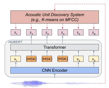
Fig. 1: The HuBERT approach predicts hidden cluster assignments of the masked frames ($y_{2},y_{3},y_{4}$ in the figure) generated by one or more iterations of k-means clustering.

图 1：HuBERT 方法预测由一轮或多轮 k-means 聚类生成的掩蔽帧隐聚类分配（图中 $y_{2},y_{3},y_{4}$）。

Inspired by this, we propose to use acoustic unit discovery models to provide frame-level targets. Let $X$ denote a speech utterance $X=[x_{1},\cdots,x_{T}]$ of $T$ frames. Discovered hidden units are denoted with $h(X)=Z=[z_{1},\cdots,z_{T}]$, where $z_{t}\in[C]$ is a $C$-class categorical variable and $h$ is a clustering model, e.g. k-means.

受此启发，我们提议用声学单元发现模型提供帧级目标。令 $X$ 表示 $T$ 帧的语音话语 $X=[x_{1},\cdots,x_{T}]$。发现的隐单元记为 $h(X)=Z=[z_{1},\cdots,z_{T}]$，其中 $z_{t}\in[C]$ 为 $C$ 类类别变量，$h$ 为聚类模型（例如 k-means）。

II-B Representation Learning via Masked Prediction

II-B 经由掩蔽预测的表征学习

Let $M\subset[T]$ denote the set of indices to be masked for a length-$T$ sequence $X$, and $\tilde{X}=r(X,M)$ denote a corrupted version of $X$ where $x_{t}$ is replaced with a mask embedding $\tilde{x}$ if $t\in M$. A masked prediction model $f$ takes as input $\tilde{X}$ and predicts a distribution over the target indeces at each timestep $p_{f}(\cdot\mid\tilde{X},t)$. There are two decisions to be made for masked prediction: how to mask and where to apply the prediction loss.

令 $M\subset[T]$ 为长度 $T$ 的序列 $X$ 上待掩蔽的下标集合，$\tilde{X}=r(X,M)$ 为 $X$ 的损坏版本：若 $t\in M$，则 $x_{t}$ 被替换为掩蔽嵌入 $\tilde{x}$。掩蔽预测模型 $f$ 以 $\tilde{X}$ 为输入，在每个时间步预测目标下标上的分布 $p_{f}(\cdot\mid\tilde{X},t)$。掩蔽预测有两个决定：如何掩蔽，以及在何处施加预测损失。

Regarding the first decision, we adopt the same strategies used in SpanBERT [34] and wav2vec 2.0 [6] for mask generation, where $p$% of the timesteps are randomly selected as start indices, and spans of $l$ steps are masked. To address the second decision, we denote the cross-entropy loss computed over masked and unmasked timesteps as $L_{m}$ and $L_{u}$, respectively. $L_{m}$ is defined as:

关于第一个决定，我们采用与 SpanBERT [34] 与 wav2vec 2.0 [6] 相同的掩蔽生成策略：随机选 $p\%$ 的时间步为起始下标，并掩蔽长度为 $l$ 的跨度。关于第二个决定，记在掩蔽与未掩蔽时间步上计算的交叉熵损失分别为 $L_{m}$ 与 $L_{u}$。$L_{m}$ 定义为：

$$L_{m}(f;X,M,Z)=\sum_{t\in M}\log p_{f}(z_{t}\mid\tilde{X},t), \tag{1}$$

and $L_{u}$ is of the same form except that it sums over $t\not\in M$. The final loss is computed as a weighted sum of the two terms: $L=\alpha L_{m}+(1-\alpha)L_{u}$. In the extreme case when $\alpha=0$, the loss is computed over the unmasked timesteps, which is similar to acoustic modeling in hybrid speech recognition systems [35, 36, 37, 38]. In our setup, this limits the learning process to mimicking the clustering model.

而 $L_{u}$ 形式相同，只是对 $t\notin M$ 求和。最终损失为两项加权和：$L=\alpha L_{m}+(1-\alpha)L_{u}$。极端情形 $\alpha=0$ 时，损失只在未掩蔽时间步上计算，类似混合语音识别系统中的声学建模 [35, 36, 37, 38]。在我们的设定下，这会把学习限制为模仿聚类模型。

In the other extreme with $\alpha=1$, the loss is only computed over the masked timesteps where the model has to predict the targets corresponding to the unseen frames from context, analogous to language modeling. It forces the model to learn both the acoustic representation of unmasked segments and the long-range temporal structure of the speech data. We hypothesize that the setup with $\alpha=1$ is more resilient to the quality of cluster targets, which is demonstrated in our experiments (see Table VI).

另一极端 $\alpha=1$ 时，损失只在掩蔽时间步上计算：模型必须从上下文预测未见帧对应的目标，类似语言建模。这迫使模型既学习未掩蔽段的声学表征，也学习语音数据的长程时序结构。我们假设 $\alpha=1$ 的设定对聚类目标质量更有韧性，实验也支持这一点（见后文消融）。

II-C Learning with Cluster Ensembles

II-C 用聚类集成学习

A simple idea to improve target quality is to utilize multiple clustering models. While an individual clustering model may perform terribly, cluster ensembles can provide complementary information to facilitate representation learning. For example, an ensemble of k-means models with different codebook sizes can create targets of different granularity, from manner classes (vowel/consonant) to sub-phone states (senones). To extend the proposed framework, let $Z^{(k)}$ be the target sequences generated by the $k$-th clustering model. We can now re-write $L_{m}$ as:

提升目标质量的一个简单想法是使用多个聚类模型。单个聚类可能很差，但聚类集成可提供互补信息以促进表征学习。例如，不同码本大小的 k-means 集成可产生不同粒度的目标，从发音方法类（元音/辅音）到亚音素状态（senones）。为扩展该框架，令 $Z^{(k)}$ 为第 $k$ 个聚类模型生成的目标序列，损失在多个码本上求和。

$$L_{m}(f;X,\{Z^{(k)}\}_{k},M)=\sum_{t\in M}\sum_{k}\log p_{f}^{(k)}(z_{t}^{(k)}\mid\tilde{X},t), \tag{2}$$

and similarly for the unmasked loss $L_{u}$. This is analogous to multi-task learning, but with tasks created by unsupervised clustering.

对未掩蔽损失 $L_{u}$ 亦然。这类似于多任务学习，但任务由无监督聚类创建。

Additionally, ensembling is intriguing because it can be used alongside product quantization (PQ) [39], where a feature space is partitioned into multiple subspaces, and each subspace is quantized separately. PQ allows effective Euclidean distance-based quantization such as k-means for high-dimensional features and heterogeneous features whose scale differs significantly between subspaces. In this case, the theoretical size of the target space is the product of all codebooks’ sizes.

此外，集成很有吸引力，因为它可与乘积量化（PQ）[39] 并用：特征空间划成多个子空间，各子空间分别量化。PQ 使基于欧氏距离的量化（如 k-means）能有效用于高维特征，以及各子空间尺度差异显著的异构特征。此时目标空间的理论大小是各码本大小之积。

II-D Iterative Refinement of Cluster Assignments

II-D 聚类分配的迭代精炼

In addition to using cluster ensembles, another direction for improved representation is refining the cluster assignments throughout the learning process. Since we expect a pre-trained model to provide better representations than the raw acoustic feature such as MFCCs, we can create a new generation of clusters by training a discrete latent model over the learned latent representations. The learning process then proceeds with the newly discovered units.

除聚类集成外，改进表征的另一方向是在学习过程中精炼聚类分配。由于我们预期预训练模型能提供优于 MFCC 等原始声学特征的表征，可在学到的潜表征上训练离散潜模型，生成新一代聚类；学习过程再以新发现的单元继续。

II-E Implementation

II-E 实现

Our pre-trained models follows the wav2vec 2.0 architecture [6], with a convolutional waveform encoder, a BERT encoder [19], a projection layer and a code embedding layer. We consider HuBERT in three different configurations: Base, Large, and X-Large. The fisrt two follow the architectures of wav2vec 2.0 Base and Large closely. The X-Large architecture expands the model size to about 1 billion parameters, similar to the size of the Conformer XXL model in  [40]. The waveform encoder is identical for all the three configurations, which is composed of seven 512-channel layers with strides [5,2,2,2,2,2,2] and kernel widths [10,3,3,3,3,2,2]. The BERT encoder consists of many identical transformer blocks, whose parameters along with the parameter of the subsequent projection layer are specified in Table I.

我们的预训练模型遵循 wav2vec 2.0 架构 [6]，包含卷积波形编码器、BERT 编码器 [19]、投影层与码嵌入层。我们考虑三种 HuBERT 配置：Base、Large 与 X-Large。前两种紧密跟随 wav2vec 2.0 Base 与 Large；X-Large 把规模扩到约 10 亿参数，接近 [40] 中 Conformer XXL。波形编码器在各配置中相同。

		Base	Large	X-Large
CNN Encoder	strides	5, 2, 2, 2, 2, 2, 2
kernel width	10, 3, 3, 3, 3, 2, 2
channel	512
Transformer	layer	12	24	48
embedding dim.	768	1024	1280
inner FFN dim.	3072	4096	5120
layerdrop prob	0.05	0	0
attention heads	8	16	16
Projection	dim.	256	768	1024
Num. of Params	95M	317M	964M

TABLE I: Model architecture summary for Base, Large, and X-Large HuBERT models

		Base	Large	X-Large
CNN Encoder	strides	5, 2, 2, 2, 2, 2, 2
kernel width	10, 3, 3, 3, 3, 2, 2
channel	512
Transformer	layer	12	24	48
embedding dim.	768	1024	1280
inner FFN dim.	3072	4096	5120
layerdrop prob	0.05	0	0
attention heads	8	16	16
Projection	dim.	256	768	1024
Num. of Params	95M	317M	964M

表 I：模型架构摘要

The convolutional waveform encoder generates a feature sequence at a 20ms framerate for audio sampled at 16kHz (CNN encoder down-sampling factor is 320x). The audio encoded features are then randomly masked as described in Section II-B. The BERT encoder takes as input the masked sequence and outputs a feature sequence $[o_{1},\cdots,o_{T}]$. The distribution over codewords is parameterized with

卷积波形编码器对 16kHz 采样音频以 20ms 帧率生成特征序列（CNN 下采样因子为 320×）。音频编码特征再按 II-B 节随机掩蔽。BERT 编码器以掩蔽序列为输入，输出特征序列 $[o_{1},\cdots,o_{T}]$。码字上的分布参数化为

$$p_{f}^{(k)}(c\mid\tilde{X},t)=\frac{\exp(\text{sim}(A^{(k)}o_{t},e_{c})/\tau)}{\sum_{c^{\prime}=1}^{C}\exp(\text{sim}(A^{(k)}o_{t},e_{c^{\prime}})/\tau)}, \tag{3}$$

where $A$ is the projection matrix, $e_{c}$ is the embedding for codeword $c$, $\text{sim}(\cdot,\cdot)$ computes the cosine similarity between two vectors, and $\tau$ scales the logit, which is set to 0.1. When cluster ensembles are used, one projection matrix $A^{(k)}$ is applied for each clustering model $k$.

其中 $A$ 为投影矩阵，$e_{c}$ 为码字 $c$ 的嵌入，$\text{sim}(\cdot,\cdot)$ 计算两向量余弦相似度，$\tau$ 缩放 logit，设为 0.1。使用聚类集成时，对每个聚类模型 $k$ 使用一个投影矩阵 $A^{(k)}$。

After HuBERT pre-training, We use the connectionist temporal classification (CTC) [41] loss for ASR fine-tuning of the whole model weights except the convolutional audio encoder, which remains frozen. The projection layer(s) is removed and replaced with a randomly initialized softmax layer. The CTC target vocabulary includes 26 English characters, a space token, an apostrophe, and a special CTC blank symbol.

HuBERT 预训练之后，我们用连接时序分类（CTC）[41] 损失对整模权重做 ASR 微调，卷积音频编码器保持冻结。投影层被移除，换为随机初始化的 Softmax 层。CTC 目标词表含 26 个英文字母、空格、撇号以及特殊 CTC 空白符。

III Related Work

III 相关工作

We discuss recent studies on self-supervised speech representation learning by grouping them by training objective. The earliest line of work learns representations by postulating a generative model for speech with latent variables, which are assumed to capture the relevant phonetic information. Training of these models amounts to likelihood maximization. Different latent structures have been applied to encode the prior assumption, such as continuous [29], discrete [31, 42], or sequential [30, 28, 43, 32, 33].

我们按训练目标对近期自监督语音表征学习研究分组讨论。最早的一条线通过为语音假定带潜变量的生成模型来学习表征，这些潜变量被假设捕捉相关语音信息；训练即似然最大化。已用不同潜结构编码先验，例如连续 [29]、离散 [31, 42] 或序列 [30, 28, 43, 32, 33]。

Prediction-based self-supervised learning has gathered increasing interests recently, where a model is tasked to predict the content of the unseen regions [4, 44, 45, 46, 47, 48, 49, 50] or to contrast the target unseen frame with randomly sampled ones [1, 3, 2, 6]. Some models combine both the predictive and the contrastive losses [5, 51]. These objectives can usually be interpreted as mutual information maximization [52]. Other objectives do not belong to these categories, for example, [53].

基于预测的自监督学习近来兴趣上升：模型被要求预测未见区域的内容 [4, 44, 45, 46, 47, 48, 49, 50]，或把目标未见帧与随机采样帧做对比 [1, 3, 2, 6]。有些模型同时结合预测与对比损失 [5, 51]。这些目标通常可解释为互信息最大化 [52]。也有不属于这些类别的目标，例如 [53]。

This work is most related to DiscreteBERT [51]: both HuBERT and DiscreteBERT predict discrete targets of masked regions. However, there are several crucial differences. First, instead of taking quantized units as input, HuBERT takes raw waveforms as input to pass as much information as possible to the transformer layers, which was shown to be important in [6]. Furthermore, in the experiment section, we show that our model, with simple k-means targets, can achieve better performance than DiscreteBERT that uses vq-wav2vec [5] learned units. Second, we also present many techniques to improve teacher quality instead of using a single fixed teacher as done in DiscreteBERT.

本工作与 DiscreteBERT [51] 最相关：二者都预测掩蔽区域的离散目标。但有几处关键差异。首先，HuBERT 不以量化单元为输入，而以原始波形为输入，尽量把信息送进 Transformer 层，这一点在 [6] 中被证明重要。其次，实验表明即使用简单的 k-means 目标，我们的模型也能超过使用 vq-wav2vec [5] 学得单元的 DiscreteBERT。再次，我们提出多种提升教师质量的技术，而非像 DiscreteBERT 那样使用单一固定教师。

HuBERT is also related to wav2vec 2.0 [6]. However, the latter employs a contrastive loss that requires careful design of where to sample negative frames from, an auxiliary diversity loss to encourage the discrete unit usage, and demands a proper Gumbel-softmax temperature annealing schedule. In addition, it only explores quantizing the waveform encoder output, which may not be the best feature for quantization due to the limited capacity of the convolutional encoder, as suggested by our ablation studies in Figure 2. Concretely, our proposed method adopts a more direct predictive loss by separating the acoustic unit discovery step from the masked prediction representation learning phase and achieves the state-of-the-art results that match or outperform wav2vec 2.0 on different fine-tuning scales.

HuBERT 也与 wav2vec 2.0 [6] 相关。但后者使用对比损失，需要仔细设计负样本采样位置、用辅助多样性损失鼓励离散单元使用，并要求合适的 Gumbel-softmax 温度退火日程。此外，它只探索量化波形编码器输出；由于卷积编码器容量有限，这未必是量化的最佳特征，如图 2 的消融所示。具体地，我们的方法把声学单元发现与掩蔽预测表征学习分开，采用更直接的预测损失，并在不同微调规模上达到匹配或超过 wav2vec 2.0 的结果。

Finally, the idea of iterative refinement target labels is similar to iterative pseudo labeling for semi-supervised ASR [12, 54], which leverages an improving student model to generate better pseudo-labels for the next iteration of training. The HuBERT approach can be seen as extending this method to the self-supervised setup with a masked prediction loss.

最后，迭代精炼目标标签的想法类似于半监督 ASR 的迭代伪标签 [12, 54]：利用不断改进的学生模型为下一轮训练生成更好伪标签。HuBERT 可视为把该方法扩展到带掩蔽预测损失的自监督设定。

IV Experimental Details

IV 实验细节

IV-A Data

IV-A 数据

For unsupervised pre-training, we use the full 960 hours of LibriSpeech audio [24] or 60,000 hours of Libri-light [25] audio, both of which are derived from the LibriVox project that contains English recordings of copyright-free audiobooks by volunteers from the Internet. For supervised fine-tuning, five different partitions are considered: Libri-light 10-minute, 1-hour, 10-hour splits and LibriSpeech 100-hour (train-clean-100) and 960-hour (train-clean-100, train-clean-360, train-other-500 combined) splits. The three Libri-light splits are subsets of the the LibriSpeech training split, and each of them contain half of the audio from train-clean-* and the other from train-other-500.

无监督预训练使用完整 960 小时 LibriSpeech 音频 [24] 或 6 万小时 Libri-light 音频 [25]，二者均来自 LibriVox：互联网志愿者录制的无版权英文有声书。有监督微调考虑五个划分：Libri-light 的 10 分钟、1 小时、10 小时划分，以及 LibriSpeech 的 100 小时（train-clean-100）与 960 小时（train-clean-100、train-clean-360、train-other-500 合并）划分。三个 Libri-light 划分是 LibriSpeech 训练划分的子集，各自一半来自 train-clean-*，一半来自 train-other-500。

IV-B Unsupervised Unit Discovery

IV-B 无监督单元发现

To demonstrate the effectiveness of the proposed method on utilizing low-quality cluster assignments, we consider the k-means algorithm [55] for acoustic unit discovery by default. It is one of the most naive unit discovery models that can be treated as modeling an isotropic Gaussian with the same scalar variance for each acoustic unit. To generate labels for the first iteration HuBERT training over the 960 hour LibriSpeech training set, we run k-means clustering with 100 clusters on 39-dimensional MFCC features, which are 13 coefficients with the first and the second-order derivatives.

为展示所提方法在利用低质量聚类分配上的有效性，默认用 k-means [55] 做声学单元发现。它是最朴素的单元发现模型之一，可视为为每个声学单元建模具有相同标量方差的各向同性高斯。为给 960 小时 LibriSpeech 训练集上的第一轮 HuBERT 训练生成标签，我们在 39 维 MFCC 特征（13 个系数及其一阶、二阶导数）上跑 100 类 k-means。

To generate better targets for the subsequent iterations, we run k-means clustering with 500 clusters on the latent features extracted from the HuBERT model pre-trained in the previous iteration (not fine-tuned) at some intermediate transformer layer. Since the feature dimension at the transformer output is much higher than the MFCC features (768-D for HuBERT Base), we cannot afford to load the entire 960 hour training split to the memory. So instead, we randomly sample 10% of the data for fitting the k-means model.

为给后续迭代生成更好目标，我们在上一轮预训练（未微调）的 HuBERT 模型某一中间 Transformer 层提取的潜特征上，跑 500 类 k-means。由于 Transformer 输出维远高于 MFCC（HuBERT Base 为 768 维），无法把整个 960 小时训练划分载入内存，因此随机采样 10% 数据拟合 k-means。

The MiniBatchKMeans algorithm implemented in the scikit-learn [56] package is used for clustering, which fits a mini-batch of samples at a time.[^2] We set the mini-batch size to be 10,000 frames. k-means++ [57] with 20 random starts is used for better initialization.

聚类使用 scikit-learn [56] 中的 MiniBatchKMeans，每次拟合一个 mini-batch 样本。[^2] mini-batch 大小设为 10000 帧。为更好初始化，使用带 20 次随机重启的 k-means++ [57]。

IV-C Pre-Training

IV-C 预训练

We train the Base model for two iterations on the 960 hours of LibriSpeech audio on 32 GPUs, with a batch size of at most 87.5 seconds of audio per GPU. The first iteration is trained for 250k steps, while the second iteration is trained for 400k steps using labels generated by clustering the 6-th transformer layer output of the first iteration model. Training for 100k steps takes about 9.5 hours.

我们在 32 块 GPU 上、用 960 小时 LibriSpeech 音频训练 Base 模型两轮，每卡 batch 最多约 87.5 秒音频。第一轮训练 25 万步；第二轮用对第一轮模型第 6 层 Transformer 输出聚类得到的标签训练 40 万步。每 10 万步大约需要 9.5 小时。

Next we train HuBERT Large and X-Large for one iteration on 60,000 hours of Libri-light audio on 128 and 256 GPUs, respectively, for 400k steps. The batch sizes are reduced to 56.25 and 22.5 seconds of audio per GPU due to memory constraints. Instead of restarting the iterative process from clustering MFCC features, we extract features from the 9-th transformer layer of the second iteration Base HuBERT for clustering and use those labels for training these two models. Hence, these two models can also be seen as the third iteration models.

随后在 6 万小时 Libri-light 上分别用 128 与 256 块 GPU 训练 HuBERT Large 与 X-Large 各一轮，共 40 万步。受内存限制，每卡 batch 分别降为约 56.25 与 22.5 秒音频。我们不再从 MFCC 聚类重启迭代，而是从第二轮 Base HuBERT 的第 9 层提取特征做聚类，并用这些标签训练这两个模型；因此它们也可视为第三轮模型。

For all HuBERT configurations, mask span is set to $l=10$, and $p=8\%$ of the waveform encoder output frames are randomly selected as mask start if not otherwise mentioned. Adam [58] optimizer is used with $\beta=(0.9,0.98)$, and the learning rate ramps up linearly from 0 to the peak learning rate for the first 8% of the training steps, and then decays linearly back to zero. The peak learning rates are 5e-4/1.5e-3/3e-3 for Base/Large/X-Large models.

对所有 HuBERT 配置，掩蔽跨度设为 $l=10$，除非另有说明，随机选波形编码器输出帧的 $p=8\%$ 作为掩蔽起点。使用 Adam [58]，$\beta=(0.9,0.98)$；学习率在前 8% 步数从 0 线性升到峰值，再线性降回 0。Base/Large/X-Large 的峰值学习率分别为 5e-4 / 1.5e-3 / 3e-3。

IV-D Supervised Fine-Tuning and Decoding

IV-D 有监督微调与解码

We fine-tune each model on 8 GPUs on the labeled splits described in Section IV-A. The batch sizes per GPU are at most 200/80/40 seconds of audio for Base/Large/X-Large models. During fine-tuning, the convolutional waveform audio encoder parameters are fixed. Like wav2vec 2.0, we introduce a freeze-step hyperparameter to control how many fine-tuning steps the transformer parameters are fixed, and only the new softmax matrix is trained. We sweep over peak learning rate ([1e-5, 1e-4]), learning rate schedule (percentage of steps for linear ramp-up and decay), number of fine-tuning steps, freeze step, and waveform encoder output masking probability for each model size and fine-tuning split combination using the word error rate (WER) on the dev-other subset as a criterion for model selection.

我们在第 IV-A 节所述有标签划分上，用 8 块 GPU 微调各模型。Base/Large/X-Large 每卡 batch 最多约 200/80/40 秒音频。微调时卷积波形编码器参数固定。与 wav2vec 2.0 一样，引入 freeze-step 超参控制前多少微调步只训练新 Softmax 矩阵、Transformer 参数保持固定。对每种模型规模与微调划分组合，以 dev-other 上的词错误率（WER）为准则，扫描峰值学习率（[1e-5, 1e-4]）、学习率日程（线性升温与衰减步数比例）、微调步数、freeze step，以及波形编码器输出掩蔽概率。

We use the wav2letter++ [59] beam search decoder wrapped in Fairseq [60] for language model-fused decoding, which optimizes:

我们使用封装在 Fairseq [60] 中的 wav2letter++ [59] 束搜索解码器做语言模型融合解码，优化：

$$\log p_{CTC}(Y\mid X)+w_{1}\log P_{LM}(Y)+w_{2}|Y|, \tag{4}$$

where $Y$ is the predicted text, $|Y|$ is the length of the text, and $w_{1}$ and $w_{2}$ denote the language model weight and word score. The decoding hyperparameters are searched with Ax, a Bayesian optimization toolkit,[^3]. In this work, we consider both $n$-gram and transformer language models trained on the official Librispeech language modeling data.

其中 $Y$ 为预测文本，$|Y|$ 为文本长度，$w_{1}$ 与 $w_{2}$ 分别表示语言模型权重与词分数。解码超参用贝叶斯优化工具包 Ax 搜索。[^3] 本文同时考虑在官方 Librispeech 语言建模数据上训练的 $n$-gram 与 Transformer 语言模型。

IV-E Metrics of Target Quality

IV-E 目标质量指标

For analysis, we derive frame-level forced-aligned phonetic transcripts using a hybrid ASR system to measure the correlation between the k-means cluster assignments and the actual phonetic units. Given aligned frame-level phonetic labels $[y_{1},\cdots,y_{T}]$ and k-means labels $[z_{1},\cdots,z_{T}]$, the joint distribution between the two variables $p_{yz}(i,j)$ can be estimated by counting the occurrences:

为分析起见，我们用混合 ASR 系统得到帧级强制对齐音素转录，以衡量 k-means 聚类分配与真实音素单元之间的相关。给定对齐的帧级音素标签 $[y_{1},\cdots,y_{T}]$ 与 k-means 标签 $[z_{1},\cdots,z_{T}]$，两变量的联合分布 $p_{yz}(i,j)$ 可通过计数估计：

$$p_{yz}(i,j)=\dfrac{\sum_{t=1}^{T}[y_{t}=i\wedge z_{t}=j]}{T}, \tag{5}$$

where $i$ denotes the $i$-th phoneme class and $j$ denotes the $j$-th k-means label class. The marginal probabilities are computed as $p_{z}(j)=\sum_{i}p_{yz}(i,j)$ and $p_{y}(j)=\sum_{j}p_{yz}(i,j)$.

其中 $i$ 表示第 $i$ 个音素类，$j$ 表示第 $j$ 个 k-means 标签类。边缘概率为 $p_{z}(j)=\sum_{i}p_{yz}(i,j)$，$p_{y}(i)=\sum_{j}p_{yz}(i,j)$。

For each phone class $i$, we further compute the most likely target label as:

对每个音素类 $i$，进一步计算最可能的目标标签为：

$$z^{*}(i)=\arg\max_{j}p_{yz}(i,j). \tag{6}$$

Likewise, for each k-means class $j$, we compute the most likely phone label as:

同样，对每个 k-means 类 $j$，计算最可能的音素标签为：

$$y^{*}(j)=\arg\max_{i}p_{yz}(i,j). \tag{7}$$

Three metrics are considered:

考虑三个指标：

1. phone purity (Phn Pur.): $$\mathbb{E}_{p_{z}(j)}[p_{y\mid z}(y^{*}(j)\mid j)],$$ (8) where $p_{y\mid z}(i\mid j)=p_{yz}(i,j)/p_{z}(j)$ denotes the conditional probability of phone given a k-means label. This metric measures the average phone purity within one class, which can be interpreted as the frame-level phone accuracy if we transcribe each k-means class with its most likely phone label. When comparing different sets of target labels with the same number of units, higher purity indicates better quality. However, this metric is less meaningful when comparing two sets with different numbers of units: in the extreme case where each frame is assigned a unique target label, the phone purity would be 100%.

1. 音素纯度（Phn Pur.）：$$\mathbb{E}_{p_{z}(j)}[p_{y\mid z}(y^{*}(j)\mid j)],$$ (8) 其中 $p_{y\mid z}(i\mid j)=p_{yz}(i,j)/p_{z}(j)$ 表示给定 k-means 标签时音素的条件概率。该指标衡量一类内的平均音素纯度，可解释为：若用最可能音素转写每个 k-means 类，得到的帧级音素准确率。在单元数相同的不同目标标签集合之间比较时，纯度越高质量越好。但比较单元数不同的两套标签时该指标意义较弱：极端情况下每帧一个唯一目标，音素纯度会是 100%。

2. cluster purity (Cls Pur.): $$\mathbb{E}_{p_{y}(i)}[p_{z\mid y}(z^{*}(i)\mid i)],$$ (9) where $p_{z\mid y}(j\mid i)=p_{yz}(i,j)/p_{y}(i)$ denotes the conditional probability of a k-means label given phone label. Cluster purity is the counterpart of phone purity, whose value would typically decrease when the number of units increases. When comparing target labels with the same number of units, higher cluster purity also indicates a better quality, as frames of the same phone are more likely labeled as the same k-means label class.

2. 聚类纯度（Cls Pur.）：$$\mathbb{E}_{p_{y}(i)}[p_{z\mid y}(z^{*}(i)\mid i)],$$ (9) 其中 $p_{z\mid y}(j\mid i)=p_{yz}(i,j)/p_{y}(i)$ 表示给定音素标签时 k-means 标签的条件概率。聚类纯度是音素纯度的对偶；单元数增加时其值通常下降。在单元数相同的目标之间比较时，聚类纯度越高也表示质量越好，因为同一音素的帧更可能落入同一聚类。

3. phone-normalized mutual information (PNMI): $\displaystyle\dfrac{I(y;z)}{H(y)}$ $\displaystyle=\dfrac{\sum_{i}\sum_{j}p_{yz}(i,j)\log\dfrac{p_{yz}(i,j)}{p_{y}(i)p_{z}(j)}}{\sum_{i}p_{y}(i)\log p_{y}(i)}$ (10) $\displaystyle=\dfrac{H(y)-H(y\mid z)}{H(y)}$ (11) $\displaystyle=1-\dfrac{H(y\mid z)}{H(y)}.$ (12) PNMI is an information-theoretic metric that measures the percentage of uncertainty about the phone label $y$ eliminated after observing the k-means label $z$. Higher PNMI also indicates better k-means clustering quality.

3. 音素归一化互信息（PNMI）：$\displaystyle\dfrac{I(y;z)}{H(y)}$。PNMI 是信息论指标，衡量观察到 k-means 标签 $z$ 后关于音素标签 $y$ 的不确定性被消除的比例；越高通常表示目标质量越好。

Model	Unlabeled Data	LM	dev-clean	dev-other	test-clean	test-other
10-min labeled
DiscreteBERT [51]	LS-960	4-gram	15.7	24.1	16.3	25.2
wav2vec 2.0 Base [6]	LS-960	4-gram	8.9	15.7	9.1	15.6
wav2vec 2.0 Large [6]	LL-60k	4-gram	6.3	9.8	6.6	10.3
wav2vec 2.0 Large [6]	LL-60k	Transformer	4.6	7.9	4.8	8.2
HUBERT Base	LS-960	4-gram	9.1	15.0	9.7	15.3
HUBERT Large	LL-60k	4-gram	6.1	9.4	6.6	10.1
HUBERT Large	LL-60k	Transformer	4.3	7.0	4.7	7.6
HUBERT X-Large	LL-60k	Transformer	4.4	6.1	4.6	6.8
1-hour labeled
DeCoAR 2.0 [50]	LS-960	4-gram	-	-	13.8	29.1
DiscreteBERT [51]	LS-960	4-gram	8.5	16.4	9.0	17.6
wav2vec 2.0 Base [6]	LS-960	4-gram	5.0	10.8	5.5	11.3
wav2vec 2.0 Large [6]	LL-60k	Transformer	2.9	5.4	2.9	5.8
HUBERT Base	LS-960	4-gram	5.6	10.9	6.1	11.3
HUBERT Large	LL-60k	Transformer	2.6	4.9	2.9	5.4
HUBERT X-Large	LL-60k	Transformer	2.6	4.2	2.8	4.8
10-hour labeled
SlimIPL [54]	LS-960	4-gram + Transformer	5.3	7.9	5.5	9.0
DeCoAR 2.0 [50]	LS-960	4-gram	-	-	5.4	13.3
DiscreteBERT [51]	LS-960	4-gram	5.3	13.2	5.9	14.1
wav2vec 2.0 Base [6]	LS-960	4-gram	3.8	9.1	4.3	9.5
wav2vec 2.0 Large [6]	LL-60k	Transformer	2.4	4.8	2.6	4.9
HUBERT Base	LS-960	4-gram	3.9	9.0	4.3	9.4
HUBERT Large	LL-60k	Transformer	2.2	4.3	2.4	4.6
HUBERT X-Large	LL-60k	Transformer	2.1	3.6	2.3	4.0
100-hour labeled
IPL [12]	LL-60k	4-gram + Transformer	3.19	6.14	3.72	7.11
SlimIPL [54]	LS-860	4-gram + Transformer	2.2	4.6	2.7	5.2
Noisy Student[61]	LS-860	LSTM	3.9	8.8	4.2	8.6
DeCoAR 2.0 [50]	LS-960	4-gram	-	-	5.0	12.1
DiscreteBERT [51]	LS-960	4-gram	4.0	10.9	4.5	12.1
wav2vec 2.0 Base [6]	LS-960	4-gram	2.7	7.9	3.4	8.0
wav2vec 2.0 Large [6]	LL-60k	Transformer	1.9	4.0	2.0	4.0
HUBERT Base	LS-960	4-gram	2.7	7.8	3.4	8.1
HUBERT Large	LL-60k	Transformer	1.8	3.7	2.1	3.9
HUBERT X-Large	LL-60k	Transformer	1.7	3.0	1.9	3.5

TABLE II: Results and comparison with the literature on low resource setups (10-min, 1-hour, 10-hour, and 100-hour of labeled data).

Model	Unlabeled Data	LM	dev-clean	dev-other	test-clean	test-other
10-min labeled
DiscreteBERT [51]	LS-960	4-gram	15.7	24.1	16.3	25.2
wav2vec 2.0 Base [6]	LS-960	4-gram	8.9	15.7	9.1	15.6
wav2vec 2.0 Large [6]	LL-60k	4-gram	6.3	9.8	6.6	10.3
wav2vec 2.0 Large [6]	LL-60k	Transformer	4.6	7.9	4.8	8.2
HUBERT Base	LS-960	4-gram	9.1	15.0	9.7	15.3
HUBERT Large	LL-60k	4-gram	6.1	9.4	6.6	10.1
HUBERT Large	LL-60k	Transformer	4.3	7.0	4.7	7.6
HUBERT X-Large	LL-60k	Transformer	4.4	6.1	4.6	6.8
1-hour labeled
DeCoAR 2.0 [50]	LS-960	4-gram	-	-	13.8	29.1
DiscreteBERT [51]	LS-960	4-gram	8.5	16.4	9.0	17.6
wav2vec 2.0 Base [6]	LS-960	4-gram	5.0	10.8	5.5	11.3
wav2vec 2.0 Large [6]	LL-60k	Transformer	2.9	5.4	2.9	5.8
HUBERT Base	LS-960	4-gram	5.6	10.9	6.1	11.3
HUBERT Large	LL-60k	Transformer	2.6	4.9	2.9	5.4
HUBERT X-Large	LL-60k	Transformer	2.6	4.2	2.8	4.8
10-hour labeled
SlimIPL [54]	LS-960	4-gram + Transformer	5.3	7.9	5.5	9.0
DeCoAR 2.0 [50]	LS-960	4-gram	-	-	5.4	13.3
DiscreteBERT [51]	LS-960	4-gram	5.3	13.2	5.9	14.1
wav2vec 2.0 Base [6]	LS-960	4-gram	3.8	9.1	4.3	9.5
wav2vec 2.0 Large [6]	LL-60k	Transformer	2.4	4.8	2.6	4.9
HUBERT Base	LS-960	4-gram	3.9	9.0	4.3	9.4
HUBERT Large	LL-60k	Transformer	2.2	4.3	2.4	4.6
HUBERT X-Large	LL-60k	Transformer	2.1	3.6	2.3	4.0
100-hour labeled
IPL [12]	LL-60k	4-gram + Transformer	3.19	6.14	3.72	7.11
SlimIPL [54]	LS-860	4-gram + Transformer	2.2	4.6	2.7	5.2
Noisy Student[61]	LS-860	LSTM	3.9	8.8	4.2	8.6
DeCoAR 2.0 [50]	LS-960	4-gram	-	-	5.0	12.1
DiscreteBERT [51]	LS-960	4-gram	4.0	10.9	4.5	12.1
wav2vec 2.0 Base [6]	LS-960	4-gram	2.7	7.9	3.4	8.0
wav2vec 2.0 Large [6]	LL-60k	Transformer	1.9	4.0	2.0	4.0
HUBERT Base	LS-960	4-gram	2.7	7.8	3.4	8.1
HUBERT Large	LL-60k	Transformer	1.8	3.7	2.1	3.9
HUBERT X-Large	LL-60k	Transformer	1.7	3.0	1.9	3.5

表 II： Results and comparison with the literature on low resource setups (10-min, 1-hour, 10-hour, and 100-hour of labeled data).

Model	Unlabeled Data	LM	dev-clean	dev-other	test-clean	test-other
Superivsed
Conformer L [62]	-	LSTM	-	-	1.9	3.9
Self-Training
IPL [12]	LL-60k	4-gram + Transformer	1.85	3.26	2.10	4.01
Noisy Student [61]	LV-60k	LSTM	1.6	3.4	1.7	3.4
Pre-Training
wav2vec 2.0 Large [6]	LL-60k	Transformer	1.6	3.0	1.8	3.3
pre-trained Conformer XXL [40]	LL-60k	LSTM	1.5	3.0	1.5	3.1
Pre-Training + Self-Training
wav2vec 2.0 + self-training [63]	LL-60k	Transformer	1.1	2.7	1.5	3.1
pre-trained Conformer XXL + Noisy Student [40]	LL-60k	LSTM	1.3	2.6	1.4	2.6
This work (Pre-Training)
HUBERT Large	LL-60k	Transformer	1.5	3.0	1.9	3.3
HUBERT X-Large	LL-60k	Transformer	1.5	2.5	1.8	2.9

TABLE III: Comparison with the literature on high resource setups using all 960 hours of labeled LibriSpeech data.

Model	Unlabeled Data	LM	dev-clean	dev-other	test-clean	test-other
Superivsed
Conformer L [62]	-	LSTM	-	-	1.9	3.9
Self-Training
IPL [12]	LL-60k	4-gram + Transformer	1.85	3.26	2.10	4.01
Noisy Student [61]	LV-60k	LSTM	1.6	3.4	1.7	3.4
Pre-Training
wav2vec 2.0 Large [6]	LL-60k	Transformer	1.6	3.0	1.8	3.3
pre-trained Conformer XXL [40]	LL-60k	LSTM	1.5	3.0	1.5	3.1
Pre-Training + Self-Training
wav2vec 2.0 + self-training [63]	LL-60k	Transformer	1.1	2.7	1.5	3.1
pre-trained Conformer XXL + Noisy Student [40]	LL-60k	LSTM	1.3	2.6	1.4	2.6
This work (Pre-Training)
HUBERT Large	LL-60k	Transformer	1.5	3.0	1.9	3.3
HUBERT X-Large	LL-60k	Transformer	1.5	2.5	1.8	2.9

表 III： Comparison with the literature on high resource setups using all 960 hours of labeled LibriSpeech data.

V Results

V 结果

V-A Main Results: Low- and High-Resource Setups

V-A 主结果：低资源与高资源设定

Table II presents results for the low-resource setup, where pre-trained models are fine-tuned on 10 minutes, 1 hour, 10 hours, or 100 hours of labeled data. We include comparison with semi-supervised (iterative pseudo labeling (IPL) [12], slimIPL [54], noisy student [61]) and self-supervised approaches (DeCoAR 2.0 [50], DiscreteBERT [51], wav2vec 2.0 [6]) in the literature. Increasing the amount of unlabeled data and increasing the model size improve performance, demonstrating the scalability of the proposed HuBERT self-supervised pre-training method. In the ultra-low resource setup with just 10 minutes of labeled data, the HuBERT Large model can achieve a WER of 4.7% on the test-clean set and 7.6% on the test-other set, which is 0.1% and 0.6% WER lower, respectively than the state-of-the-art wav2vec 2.0 Large model. By further scaling up the model size to 1B parameters, the HuBERT X-Large model can further reduce the WER to 4.6% and 6.8% on test-clean and test-other. The superiority of HuBERT persists across setups with different amounts of labeled data, with the only exceptions being fine-tuning on 100 hours of labeled data, where HuBERT Large is 0.1% WER higher than wav2vec 2.0 Large on test-clean, and HuBERT Base is 0.1% WER higher than wav2vec 2.0 Base on test-other. In addition, HuBERT also outperforms DiscreteBERT by a large margin in all setups, while both are trained with a virtually identical objective - masked prediction of discovered units. The considerable performance gap suggests two things. First, using waveform as the input to the model is crucial for avoiding loss of information during quantization. Second, while vq-wav2vec [5], the units that DiscreteBERT uses for training, may discover better units than k-means clustering of MFCC features, the proposed iterative refinement benefits from the improving HuBERT model and learn better units eventually. We will verify these statements in the ablation study sections.

表 II 给出主结果。我们报告在 Librispeech 与 Libri-light 预训练、并在 10 分钟至 960 小时有标签子集上微调后的 WER。HuBERT Base（960h 预训练）在各微调规模上匹配或超过 wav2vec 2.0 Base；在 Libri-light 上训练的 Large 与 X-Large 进一步降低错误率，其中 X-Large 在更具挑战的 dev-other / test-other 上相对 Large 最高约有 19% / 13% 的相对 WER 下降。结果表明：聚类–掩蔽预测范式在低资源到高资源设定下均可扩展，且迭代精炼目标能转化为可观的识别收益。

We report results of fine-tuning HuBERT models on the full 960 hours of Librispeech data and compare with the literature in Table III. Prior studies using additional unpaired speech are classified into:

我们还与下列半监督与自监督范式对照：

1. self-training: first train an ASR on labeled data to annotate unlabeled speech, and then combine both golden and ASR-annotated text-speech pairs for supervised training.

1. 自训练：先在有标签数据上训练 ASR 以标注无标签语音，再把金标与 ASR 标注的文本–语音对合并做有监督训练。

2. pre-training: first use unlabeled speech for pre-training a model, and then fine-tune the model on labeled data with a supervised training objective.

2. 预训练：先用无标签语音预训练模型，再在有标签数据上用有监督目标微调。

3. pre-training + self-training: first pre-train and fine-tune a model, and then use it to annotate unlabeled speech for self-training combined with supervised data.

3. 预训练 + 自训练：先预训练并微调一个模型，再用它标注无标签语音，与有监督数据合并做自训练。

HuBERT outperforms the state-of-the-art supervised and self-training methods and is on par with the two best pre-training results in the literature; both are based on wav2vec 2.0 contrastive learning. In contrast, it lags behind methods combining pre-training with self-training. However, as observed in [63] and [40], we expect that HuBERT can achieve comparable or better performance after combining with self-training, since the pre-trained HuBERT model is on par or better than the pre-trained model those two methods use for pseudo labeling.

总体而言，仅预训练的 HuBERT 已具强竞争力；与自训练结合时可进一步受益，说明表征学习与伪标签流水线互补。

V-B Analysis: K-Means Stability

V-B 分析：K-means 稳定性

To better understand why masked prediction of discovered units is effective, we conduct a series of analyses and ablation studies. We start with probing the stability of the k-means clustering algorithm concerning different numbers of clusters and different sizes of its training data. Two features are considered: 39-dimensional MFCC features and 768-dimensional output from the 6-th transformer layer of the first iteration HuBERT-Base model. These two features are used to produce cluster assignments for the first and the second iteration HUBERT training, respectively.

我们评估 k-means 作为无监督单元发现算法的稳定性。考虑两类特征：39 维 MFCC，以及第一轮 HuBERT-Base 第 6 层 Transformer 的 768 维输出。这两类特征分别用于生成第一轮与第二轮 HuBERT 训练的聚类分配。

For k-means clustering, we consider $K=\{100,500\}$ clusters fitted on {1, 10, 100} hours of speech sampled from the LibriSpeech training split. Each combination of the hyperparameters and the features are trained for 10 trials, and the mean and standard deviation of the supervised PNMI metric on the development set (combining dev-clean and dev-other from LibriSpeech) is reported in Table IV. The results show that the k-means clustering is reasonably stable given the small standard deviations across different hyperparameters and features. Furthermore, increasing the amount of data used for fitting k-means models improves PNMI in general, but the gain is only as much as 0.012, suggesting the feasibility of using k-means for unit discovery even with limited CPU memory relative to the feature matrix size. Lastly, the PNMI score is much higher when clustering on HuBERT features than clustering on MFCC features, and the gap is even larger with 500 clusters, indicating that iterative refinement significantly improves the clustering quality.

对 k-means，我们考虑在从 LibriSpeech 训练划分采样的 {1, 10, 100} 小时语音上拟合 $K\in\{100,500\}$ 类。每种超参与特征组合训练 10 次试验，在开发集（合并 Librispeech 的 dev-clean 与 dev-other）上报告有监督 PNMI 的均值与标准差，见表 IV。结果显示：不同超参与特征下标准差很小，k-means 相当稳定。增加拟合数据量通常提升 PNMI，但增益最多约 0.012，说明即便相对特征矩阵 CPU 内存有限，用 k-means 做单元发现仍可行。最后，在 HuBERT 特征上聚类的 PNMI 远高于 MFCC，且在 500 类时差距更大，表明迭代精炼显著提升聚类质量。

feature	C	PNMI (mean $\pm$ std) with K-means Training Size =
1h	10h	100h
MFCC	100	0.251 $\pm$ 0.001	0.253 $\pm$ 0.001	0.253 $\pm$ 0.001
500	0.283 $\pm$ 0.001	0.285 $\pm$ 0.000	0.287 $\pm$ 0.001
Base-it1-L6	100	0.563 $\pm$ 0.012	0.561 $\pm$ 0.012	0.575 $\pm$ 0.008
500	0.680 $\pm$ 0.005	0.684 $\pm$ 0.003	0.686 $\pm$ 0.004

TABLE IV: Stability of K-means as an unsupervised unit discovery algorithm with respect to different features, numbers of clusters, and training data sizes. PNMI stands for phone-normalized mutual information.

feature	C	PNMI (mean $\pm$ std) with K-means Training Size =
1h	10h	100h
MFCC	100	0.251 $\pm$ 0.001	0.253 $\pm$ 0.001	0.253 $\pm$ 0.001
500	0.283 $\pm$ 0.001	0.285 $\pm$ 0.000	0.287 $\pm$ 0.001
Base-it1-L6	100	0.563 $\pm$ 0.012	0.561 $\pm$ 0.012	0.575 $\pm$ 0.008
500	0.680 $\pm$ 0.005	0.684 $\pm$ 0.003	0.686 $\pm$ 0.004

表 IV： k-means 作为无监督单元发现算法相对不同特征、聚类数与训练数据量的稳定性。PNMI 表示音素归一化互信息。

teacher	C	PNMI	dev-other WER (%)
$\alpha=1.0$	$\alpha=0.5$	$\alpha=0.0$
Chenone (supervised top-line)	8976	0.809	10.38	9.16	9.79
K-means on MFCC	50	0.227	18.68	31.07	94.60
100	0.243	17.86	29.57	96.37
500	0.276	18.40	33.42	97.66
K-means on Base-it1-layer6	500	0.637	11.91	13.47	23.29
K-means on Base-it2-layer9	500	0.704	10.75	11.59	13.79

teacher	WER
K-means {50,100}	17.81
K-means {50,100,500}	17.56
Product K-means-0-100	19.26
Product K-means-1-100	17.64
Product K-means-2-100	18.46
Product K-means-{0,1,2}-100	16.73

TABLE V: The effect of the training objective and clustering quality on performance. $C$ refers to the number of units, and $\alpha$ is the weight for masked frames.

teacher	C	PNMI	dev-other WER (%)
$\alpha=1.0$	$\alpha=0.5$	$\alpha=0.0$
Chenone (supervised top-line)	8976	0.809	10.38	9.16	9.79
K-means on MFCC	50	0.227	18.68	31.07	94.60
100	0.243	17.86	29.57	96.37
500	0.276	18.40	33.42	97.66
K-means on Base-it1-layer6	500	0.637	11.91	13.47	23.29
K-means on Base-it2-layer9	500	0.704	10.75	11.59	13.79

teacher	WER
K-means {50,100}	17.81
K-means {50,100,500}	17.56
Product K-means-0-100	19.26
Product K-means-1-100	17.64
Product K-means-2-100	18.46
Product K-means-{0,1,2}-100	16.73

表 V： 训练目标与聚类质量对表现的影响。$C$ 为单元数，$\alpha$ 为掩蔽帧权重。

Fig. 2: Quality of the cluster assignments obtained by running k-means clustering on features extracted from each transformer layer of the first and the second iteration Base HuBERT models.

图 2：在第一轮与第二轮 Base HuBERT 各 Transformer 层提取特征上跑 k-means 所得聚类分配的质量。

V-C Analysis: Clustering Quality Across Layers and Iterations

V-C 分析：跨层与跨迭代的聚类质量

We next study how each layer of the HuBERT model from each iteration performs when used for clustering to generate training targets. The two Base HuBERT models from the first two iterations as described in Section IV-C are considered, which are referred to as Base-it1 and Base-it2, respectively. There are 26 features representing 12 transformer layers plus the input to the first transformer layer (denoted as “Layer 0”) from the two HuBERT models. For each feature, we fit three k-means models ($K=\{100,500,1000\}$ clusters) on a 100 hour subset randomly sampled from the LibriSpeech training data. The teacher quality measured in cluster purity, phone purity, and phone normalized mutual information (PNMI) is shown in Figure 2. As a baseline, MFCC achieves (cluster purity, phone purity, PNMI) = (0.099, 0.335, 0.255) for $K=100$ and (0.031, 0.356, 0.287) for $K=500$.

我们接着研究每一轮、每一层 HuBERT 特征用于聚类生成训练目标时的表现。考虑第 IV-C 节所述前两轮 Base 模型，分别记为 Base-it1 与 Base-it2。共 26 组特征：两个模型各自 12 个 Transformer 层，外加第一层 Transformer 的输入（记为“Layer 0”）。对每个特征，在从 LibriSpeech 训练数据随机采样的 100 小时子集上拟合三个 k-means（$K\in\{100,500,1000\}$）。以聚类纯度、音素纯度与 PNMI 衡量的教师质量见图 2。作为基线，MFCC 在 $K=100$ 时为（聚类纯度, 音素纯度, PNMI）=（0.099, 0.335, 0.255），$K=500$ 时为（0.031, 0.356, 0.287）。

Both Base-it1 and Base-it2 features result in significantly better clustering quality on all three metrics than MFCC with the same number of clusters. On the other hand, the best Base-it2 feature is better than the best Base-it1 on phone purity and PNMI, but slightly worse on cluster purity. Finally, we observe different trends across layers from Base-it1 and Base-it2: while Base-it2 model features generally improve over layers, Base-it1 has the best features in the middle layers around the 6th layer. Interestingly, the quality of the last few layers degrades dramatically for Base-it1, potentially because it is trained on target assignments of worse quality, and therefore the last few layers learn to mimic their bad label behavior.

在相同聚类数下，Base-it1 与 Base-it2 特征在三项指标上均显著优于 MFCC。另一方面，最好的 Base-it2 特征在音素纯度与 PNMI 上优于最好的 Base-it1，在聚类纯度上略差。最后，两轮模型跨层趋势不同：Base-it2 特征大体随层提升，而 Base-it1 在约第 6 层的中部最好。有趣的是，Base-it1 最后几层质量急剧下降，可能因为它在较差目标分配上训练，最后几层学会模仿那些糟糕标签的行为。

V-D Ablation: The Importance of Predicting Masked Frames

V-D 消融：预测掩蔽帧的重要性

We present a series of ablation studies in the following sections to learn how pre-training objective, cluster quality, and hyperparameters affect the performance. The models for ablation studies are pre-trained for 100k steps and fine-tuned on the 10-hour libri-light split using fixed hyperaprameters. MFCC-based k-means units with C=100 are used if not otherwise mentioned. We report WERs on the dev-other set decoded with the $n$-gram language model using fixed decoding hyperparameters.

后续几节给出一系列消融，考察预训练目标、聚类质量与超参如何影响表现。消融模型预训练 10 万步，并在 10 小时 Libri-light 划分上用固定超参微调。除非另有说明，使用 C=100 的基于 MFCC 的 k-means 单元。我们报告用 $n$-gram 语言模型、固定解码超参在 dev-other 上的 WER。

To understand the importance of our proposal to predict the masked frames only, we compare three conditions: 1) predicting masked frames, 2) predicting all frames, and 3) predicting unmasked frames, which can be simulated by setting $\alpha$ to 1.0, 0.5, and 0.0, respectively. We are comparing three k-means models learned from clustering MFCC teachers with 50, 100, 500 clusters, one learned from clustering HuBERT-Base-it1 6th transformer layer features, and supervised labels obtained from the forced-alignment of character-based HMM models (chenone) [64].

为理解“只预测掩蔽帧”这一提议的重要性，我们比较三种条件：1）预测掩蔽帧；2）预测所有帧；3）预测未掩蔽帧；可分别由 $\alpha$ 取 1.0、0.5、0.0 模拟。比较对象包括：在 MFCC 上聚类得到的 50/100/500 类 k-means、在 HuBERT-Base-it1 第 6 层特征上聚类得到的教师，以及由基于字符的 HMM 强制对齐得到的有监督标签（chenone）[64]。

Results shown in Table VI indicate that when learning from bad cluster assignments, computing loss only from the masked regions achieves the best performance, while the inclusion of unmasked loss results in significantly higher WERs. However, as the clustering quality improves, the model would suffer less when computing losses on the unmasked frames (Base-it1-layer6) or even achieve better performance as the case of chenone.

表 VI 显示：当从糟糕的聚类分配学习时，只在掩蔽区域计算损失表现最好，而加入未掩蔽损失会显著抬高 WER。但随着聚类质量提升，在未掩蔽帧上算损失的损害变小（Base-it1-layer6），在 chenone 情形下甚至更好。

V-E Ablation: The Effect of Cluster Ensembles

V-E 消融：聚类集成的效果

To understand the effect of combining multiple k-means models for generating targets, we consider two setups. The first one has k-means models of different numbers of clusters presented in Table VI, denoted with KM-{50,100,500}. The second one has k-means models trained on spliced MFCC features with a window of three; hence, each input feature is represented as a 117-dimensional vector. In this second case, we apply product quantization on the spliced features, where dimensions are split into the coefficients of the zeroth, first, and second-order derivatives, with each 39-dimensional subspace quantized to a codebook of 100 entries. We denote these codebooks with Product k-means-{0,1,2}-100, respectively. By comparing the results from Table VI and Table VI, it is clear that using an ensemble leads to better performance than what a single k-means clustering can achieve.

为理解组合多个 k-means 生成目标的效果，考虑两种设定。第一种是表 VI 中不同聚类数的 k-means，记为 KM-{50,100,500}。第二种在窗口为三的拼接 MFCC 上训练 k-means，故每个输入为 117 维；对此做乘积量化：维数按零阶、一阶、二阶导数系数划分，每个 39 维子空间量化为 100 项码本，分别记为 Product k-means-{0,1,2}-100。对照表 VI 结果可见，使用集成优于单一 k-means 聚类所能达到的表现。

V-F Ablation: Impact of Hyperparameters

V-F 消融：超参数的影响

Figure 3 and Table VII studies how hyperparameters affect HuBERT pre-training. It is shown that (1) the portion of frames selected as mask start is optimal at $p=$8%; (2) increasing the batch size can significantly improve the performance; (3) training for longer consistently helps for both k-means models with C={50, 100}, and the best model achieves a WER of 11.68%. These findings are also consistent with those from BERT-like models [20]. In addition, we include a comparable result from DiscreteBERT [51] in Table VII which applies k-means to quantize the same MFCC features into 13.5k units, used as both the output and the input to the BERT model. Besides using continuous speech input rather than discrete units, We hypothesize that HuBERT achieves significantly better performance because its fewer k-means clusters of 100 or 500 help capture broad phonetic concepts without delving into inter/intra-speaker variation.

图 3 与表 VII 研究超参如何影响 HuBERT 预训练。结果显示：（1）作为掩蔽起点的帧比例在 $p=$8% 附近最优；（2）增大 batch size 能显著改善表现；（3）对 C={50,100} 的 k-means，更长训练持续有帮助，最好模型 WER 达 11.68%。这些发现也与类 BERT 模型 [20] 一致。此外，表 VII 放入 DiscreteBERT [51] 的可比结果：它对同一 MFCC 量化到 13.5k 单元，同时作为 BERT 的输出与输入。除使用连续语音输入而非离散单元外，我们推测 HuBERT 显著更好，是因为 100 或 500 类的较少 k-means 簇有助于抓住宽泛语音概念，而不陷入说话人内/间变异。

teacher	C	dev-other WER (%)
steps=100k	250k	400k	800k
K-means	50	18.68	13.65	12.40	11.82
100	17.86	12.97	12.32	11.68
[51]	13.5k	26.6

TABLE VII: Varying the number of HuBERT pre-training steps. $p$ is set to 6.5%.

teacher	C	dev-other WER (%)
steps=100k	250k	400k	800k
K-means	50	18.68	13.65	12.40	11.82
100	17.86	12.97	12.32	11.68
[51]	13.5k	26.6

表 VII： 改变 HuBERT 预训练步数。$p$ 设为 6.5%。

Fig. 3: Varying masking probability $p$ (left) and effective batch size through the number of GPUs (right).

图 3：改变掩蔽概率 $p$（左）以及通过 GPU 数量改变有效 batch size（右）。

VI Conclusion

VI 结论

This paper presents HuBERT, a speech representation learning approach that relies on predicting K-means cluster assignments of masked segments of continuous input. On both the Librispeech 960 hours and the 60,000 hours Libri-light pre-training setups, HuBERT matches or outperforms the state-of-the-art systems over all fine-tuning subsets of 10mins, 1h, 10h, 100h, and 960h. Furthermore, the learned representation quality improves dramatically with iteratively refining K-means cluster assignments using learned latent representations for a previous iteration. Finally, HuBERT scales well to a 1B transformer model showing a relative reduction in WER of up to 13% on the test-other subset. For future work, we plan to improve the HuBERT training procedure to consist of a single phase. Furthermore, given the high quality of its representations, we will consider using HuBERT pre-trained representations for multiple downstream recognition and generation tasks beyond ASR.

本文提出 HuBERT：一种依赖对连续输入掩蔽段预测 k-means 聚类分配的语音表征学习方法。在 Librispeech 960 小时与 Libri-light 6 万小时两种预训练设定下，HuBERT 在 10 分钟、1h、10h、100h、960h 全部微调子集上达到或超过当时最好系统。此外，用上一轮学到的潜表征迭代精炼 k-means 聚类分配后，表征质量显著提升。最后，HuBERT 可扩展到约 10 亿参数 Transformer，在 test-other 上相对 WER 最高下降约 13%。未来工作计划把 HuBERT 训练改进为单阶段流程；并鉴于其表征质量，考虑把预训练表征用于 ASR 之外的多种下游识别与生成任务。

References

参考文献

[1] A. v. d. Oord, Y. Li, and O. Vinyals, “Representation learning with contrastive predictive coding,” arXiv preprint arXiv:1807.03748 , 2018.

[2] S. Schneider, A. Baevski, R. Collobert, and M. Auli, “wav2vec: Unsupervised pre-training for speech recognition,” arXiv preprint arXiv:1904.05862 , 2019.

[3] E. Kharitonov, M. Rivière, G. Synnaeve, L. Wolf, P.-E. Mazaré, M. Douze, and E. Dupoux, “Data augmenting contrastive learning of speech representations in the time domain,” arXiv preprint arXiv:2007.00991 , 2020.

[4] Y.-A. Chung, W.-N. Hsu, H. Tang, and J. Glass, “An unsupervised autoregressive model for speech representation learning,” arXiv preprint arXiv:1904.03240 , 2019.

[5] A. Baevski, S. Schneider, and M. Auli, “vq-wav2vec: Self-supervised learning of discrete speech representations,” arXiv preprint arXiv:1910.05453 , 2019.

[6] A. Baevski, H. Zhou, A. Mohamed, and M. Auli, “wav2vec 2.0: A framework for self-supervised learning of speech representations,” arXiv preprint arXiv:2006.11477 , 2020.

[7] G. Zavaliagkos and T. Colthurst, “Utilizing untranscribed training data to improve performance,” in DARPA Broadcast News Transcription and Understanding Workshop , 1998.

[8] J. Ma, S. Matsoukas, O. Kimball, and R. Schwartz, “Unsupervised training on large amounts of broadcast news data,” in ICASSP , 2006.

[9] J. Kahn, A. Lee, and A. Hannun, “Self-training for end-to-end speech recognition,” in ICASSP , 2020.

[10] W.-N. Hsu, A. Lee, G. Synnaeve, and A. Hannun, “Semi-supervised speech recognition via local prior matching,” arXiv preprint arXiv:2002.10336 , 2020.

[11] A. Xiao, C. Fuegen, and A. Mohamed, “Contrastive semi-supervised learning for asr,” arXiv preprint arXiv:2103.05149 , 2021.

[12] Q. Xu, T. Likhomanenko, J. Kahn, A. Hannun, G. Synnaeve, and R. Collobert, “Iterative pseudo-labeling for speech recognition,” arXiv preprint arXiv:2005.09267 , 2020.

[13] M. Caron, I. Misra, J. Mairal, P. Goyal, P. Bojanowski, and A. Joulin, “Unsupervised learning of visual features by contrasting cluster assignments,” CoRR , vol. abs/2006.09882, 2020.

[14] X. Chen and K. He, “Exploring simple siamese representation learning,” CoRR , vol. abs/2011.10566, 2020.

[15] J. Grill, F. Strub, F. Altché, C. Tallec, P. H. Richemond, E. Buchatskaya, C. Doersch, B. Á. Pires, Z. D. Guo, M. G. Azar, B. Piot, K. Kavukcuoglu, R. Munos, and M. Valko, “Bootstrap your own latent: A new approach to self-supervised learning,” CoRR , vol. abs/2006.07733, 2020.

[16] T. B. Brown, B. Mann, N. Ryder, M. Subbiah, J. Kaplan, P. Dhariwal, A. Neelakantan, P. Shyam, G. Sastry, A. Askell, S. Agarwal, A. Herbert-Voss, G. Krueger, T. Henighan, R. Child, A. Ramesh, D. M. Ziegler, J. Wu, C. Winter, C. Hesse, M. Chen, E. Sigler, M. Litwin, S. Gray, B. Chess, J. Clark, C. Berner, S. McCandlish, A. Radford, I. Sutskever, and D. Amodei, “Language models are few-shot learners,” CoRR , vol. abs/2005.14165, 2020.

[17] Y. Liu, M. Ott, N. Goyal, J. Du, M. Joshi, D. Chen, O. Levy, M. Lewis, L. Zettlemoyer, and V. Stoyanov, “Roberta: A robustly optimized bert pretraining approach,” arXiv preprint arXiv:1907.11692 , 2019.

[18] M. Lewis, Y. Liu, N. Goyal, M. Ghazvininejad, A. Mohamed, O. Levy, V. Stoyanov, and L. Zettlemoyer, “Bart: Denoising sequence-to-sequence pre-training for natural language generation, translation, and comprehension,” arXiv preprint arXiv:1910.13461 , 2019.

[19] J. Devlin, M.-W. Chang, K. Lee, and K. Toutanova, “Bert: Pre-training of deep bidirectional transformers for language understanding,” arXiv preprint arXiv:1810.04805 , 2018.

[20] K. Clark, M.-T. Luong, Q. V. Le, and C. D. Manning, “Electra: Pre-training text encoders as discriminators rather than generators,” arXiv preprint arXiv:2003.10555 , 2020.

[21] M. E. Peters, M. Neumann, M. Iyyer, M. Gardner, C. Clark, K. Lee, and L. Zettlemoyer, “Deep contextualized word representations,” in NAACL , 2018.

[22] K. He, H. Fan, Y. Wu, S. Xie, and R. Girshick, “Momentum contrast for unsupervised visual representation learning,” in CVPR , 2020.

[23] M. Caron, P. Bojanowski, A. Joulin, and M. Douze, “Deep clustering for unsupervised learning of visual features,” in ECCV , 2018.

[24] V. Panayotov, G. Chen, D. Povey, and S. Khudanpur, “Librispeech: an asr corpus based on public domain audio books,” in ICASSP , 2015.

[25] J. Kahn et al. , “Libri-light: A benchmark for asr with limited or no supervision,” in ICASSP , 2020.

[26] C.-y. Lee and J. Glass, “A nonparametric bayesian approach to acoustic model discovery,” in ACL , 2012.

[27] L. Ondel, L. Burget, and J. Černockỳ, “Variational inference for acoustic unit discovery,” Procedia Computer Science , vol. 81, pp. 80–86, 2016.

[28] J. Ebbers, J. Heymann, L. Drude, T. Glarner, R. Haeb-Umbach, and B. Raj, “Hidden markov model variational autoencoder for acoustic unit discovery.” in INTERSPEECH , 2017.

[29] W.-N. Hsu, Y. Zhang, and J. Glass, “Learning latent representations for speech generation and transformation,” in INTERSPEECH , 2017.

[30] ——, “Unsupervised learning of disentangled and interpretable representations from sequential data,” in NeurIPS , 2017.

[31] J. Chorowski, R. J. Weiss, S. Bengio, and A. van den Oord, “Unsupervised speech representation learning using wavenet autoencoders,” IEEE/ACM transactions on audio, speech, and language processing , vol. 27, no. 12, pp. 2041–2053, 2019.

[32] S. Khurana, S. R. Joty, A. Ali, and J. Glass, “A factorial deep markov model for unsupervised disentangled representation learning from speech,” in ICASSP , 2019.

[33] S. Khurana, A. Laurent, W.-N. Hsu, J. Chorowski, A. Lancucki, R. Marxer, and J. Glass, “A convolutional deep markov model for unsupervised speech representation learning,” arXiv preprint arXiv:2006.02547 , 2020.

[34] M. Joshi, D. Chen, Y. Liu, D. S. Weld, L. Zettlemoyer, and O. Levy, “Spanbert: Improving pre-training by representing and predicting spans,” Transactions of the Association for Computational Linguistics , 2020.

[35] S. Young, “Large vocabulary continuous speech recognition: A review,” IEEE Signal Processing Magazine , vol. 13, no. 5, pp. 45–57, 1996.

[36] O. Abdel-Hamid, A.-r. Mohamed, H. Jiang, and G. Penn, “Applying convolutional neural networks concepts to hybrid nn-hmm model for speech recognition,” in 2012 IEEE international conference on Acoustics, speech and signal processing (ICASSP) . IEEE, 2012, pp. 4277–4280.

[37] D. Povey, “Discriminative training for large vocabulary speech recognition,” Ph.D. dissertation, University of Cambridge, 2005.

[38] H. A. Bourlard and N. Morgan, Connectionist speech recognition: a hybrid approach . Springer Science & Business Media, 2012, vol. 247.

[39] R. M. Gray and D. L. Neuhoff, “Quantization,” IEEE transactions on information theory , vol. 44, no. 6, pp. 2325–2383, 1998.

[40] Y. Zhang, J. Qin, D. S. Park, W. Han, C.-C. Chiu, R. Pang, Q. V. Le, and Y. Wu, “Pushing the limits of semi-supervised learning for automatic speech recognition,” arXiv preprint arXiv:2010.10504 , 2020.

[41] A. Graves, S. Fernández, F. Gomez, and J. Schmidhuber, “Connectionist temporal classification: labelling unsegmented sequence data with recurrent neural networks,” in ICML , 2006.

[42] A. van den Oord, O. Vinyals et al. , “Neural discrete representation learning,” in NeurIPS , 2017.

[43] T. Glarner, P. Hanebrink, J. Ebbers, and R. Haeb-Umbach, “Full bayesian hidden markov model variational autoencoder for acoustic unit discovery.” in INTERSPEECH , 2018.

[44] Y.-A. Chung and J. Glass, “Generative pre-training for speech with autoregressive predictive coding,” in ICASSP , 2020.

[45] ——, “Improved speech representations with multi-target autoregressive predictive coding,” arXiv preprint arXiv:2004.05274 , 2020.

[46] S. Ling, Y. Liu, J. Salazar, and K. Kirchhoff, “Deep contextualized acoustic representations for semi-supervised speech recognition,” in ICASSP , 2020.

[47] W. Wang, Q. Tang, and K. Livescu, “Unsupervised pre-training of bidirectional speech encoders via masked reconstruction,” in ICASSP , 2020.

[48] A. T. Liu, S.-w. Yang, P.-H. Chi, P.-c. Hsu, and H.-y. Lee, “Mockingjay: Unsupervised speech representation learning with deep bidirectional transformer encoders,” in ICASSP , 2020.

[49] P.-H. Chi, P.-H. Chung, T.-H. Wu, C.-C. Hsieh, S.-W. Li, and H.-y. Lee, “Audio albert: A lite bert for self-supervised learning of audio representation,” arXiv preprint arXiv:2005.08575 , 2020.

[50] S. Ling and Y. Liu, “Decoar 2.0: Deep contextualized acoustic representations with vector quantization,” arXiv preprint arXiv:2012.06659 , 2020.

[51] A. Baevski, M. Auli, and A. Mohamed, “Effectiveness of self-supervised pre-training for speech recognition,” arXiv preprint arXiv:1911.03912 , 2019.

[52] Y.-H. H. Tsai, Y. Wu, R. Salakhutdinov, and L.-P. Morency, “Self-supervised learning from a multi-view perspective,” arXiv preprint arXiv:2006.05576 , 2020.

[53] S. Pascual, M. Ravanelli, J. Serrà, A. Bonafonte, and Y. Bengio, “Learning problem-agnostic speech representations from multiple self-supervised tasks,” in INTERSPEECH , 2019.

[54] T. Likhomanenko, Q. Xu, J. Kahn, G. Synnaeve, and R. Collobert, “slimipl: Language-model-free iterative pseudo-labeling,” arXiv preprint arXiv:2010.11524 , 2020.

[55] S. Lloyd, “Least squares quantization in pcm,” IEEE transactions on information theory , vol. 28, no. 2, pp. 129–137, 1982.

[56] F. Pedregosa et al. , “Scikit-learn: Machine learning in python,” the Journal of machine Learning research , 2011.

[57] D. Arthur and S. Vassilvitskii, “k-means++: The advantages of careful seeding,” Stanford, Tech. Rep., 2006.

[58] D. P. Kingma and J. Ba, “Adam: A method for stochastic optimization,” arXiv preprint arXiv:1412.6980 , 2014.

[59] V. Pratap et al. , “wav2letter++: The fastest open-source speech recognition system,” arXiv preprint arXiv:1812.07625 , 2018.

[60] M. Ott et al. , “fairseq: A fast, extensible toolkit for sequence modeling,” in NAACL , 2019.

[61] D. S. Park, Y. Zhang, Y. Jia, W. Han, C.-C. Chiu, B. Li, Y. Wu, and Q. V. Le, “Improved noisy student training for automatic speech recognition,” arXiv preprint arXiv:2005.09629 , 2020.

[62] A. Gulati, J. Qin, C.-C. Chiu, N. Parmar, Y. Zhang, J. Yu, W. Han, S. Wang, Z. Zhang, Y. Wu et al. , “Conformer: Convolution-augmented transformer for speech recognition,” arXiv preprint arXiv:2005.08100 , 2020.

[63] Q. Xu, A. Baevski, T. Likhomanenko, P. Tomasello, A. Conneau, R. Collobert, G. Synnaeve, and M. Auli, “Self-training and pre-training are complementary for speech recognition,” arXiv preprint arXiv:2010.11430 , 2020.

[64] D. Le, X. Zhang, W. Zheng, C. Fügen, G. Zweig, and M. L. Seltzer, “From senones to chenones: Tied context-dependent graphemes for hybrid speech recognition,” in ASRU , 2019.