How much can language models memorize?
How much do language models memorize?
语言模型记住了多少?
John X. Morris Affiliation: FAIR at Meta Affiliation: Cornell University Chawin Sitawarin Affiliation: Google DeepMind Chuan Guo Affiliation: FAIR at Meta Narine Kokhlikyan Affiliation: FAIR at Meta G. Edward Suh Affiliation: Cornell University Affiliation: NVIDIA Alexander M. Rush Affiliation: Cornell University Kamalika Chaudhuri Affiliation: FAIR at Meta Saeed Mahloujifar Affiliation: FAIR at Meta
Abstract
摘要
We propose a new method for estimating how much a model “knows” about a datapoint and use it to measure the capacity of modern language models. We formally separate memorization into two components: unintended memorization, the information a model contains about a specific dataset, and generalization, the information a model contains about the true data-generation process. By eliminating generalization, we can compute the total memorization of a given model, which provides an estimate of model capacity: our measurements estimate that models in the GPT family have an approximate capacity of 3.6 bits-per-parameter. We train language models on datasets of increasing size and observe that models memorize until their capacity fills, at which point “grokking” begins, and unintended memorization decreases as models begin to generalize. We train hundreds of transformer language models ranging from to parameters and produce a series of scaling laws relating model capacity and data size to membership inference.
我们提出一种新方法,用来估计模型对某条数据「知道」多少,并据此测量现代语言模型的容量。我们把记忆形式地拆成两个部分:非预期记忆(unintended memorization)是模型中关于某个具体数据集的信息,泛化则是模型中关于真实数据生成过程的信息。去掉泛化之后,就可以算出模型的总记忆量,从而估计容量:我们的测量给出,GPT 系列模型的容量大约是每参数 3.6 比特。我们在规模逐渐增大的数据集上训练语言模型,观察到模型会一直记忆,直到容量被填满;此后开始出现「grokking」,非预期记忆下降,模型转入泛化。我们训练了数百个参数量从 到 的 Transformer 语言模型,并给出一组把模型容量、数据规模与成员推断联系起来的缩放律。
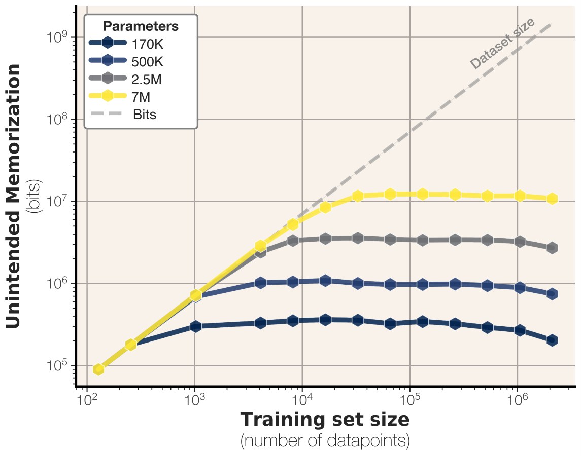
Figure 1: Unintended memorization of uniform random data (Section 3). Memorization plateaus at the empirical capacity limit of different-sized models from the GPT-family, approximately 3.6 bits-per-parameter.
图 1:均匀随机数据上的非预期记忆(第 3 节)。记忆量会在不同规模 GPT 系列模型的经验容量上限处进入平台,大约是每参数 3.6 比特。
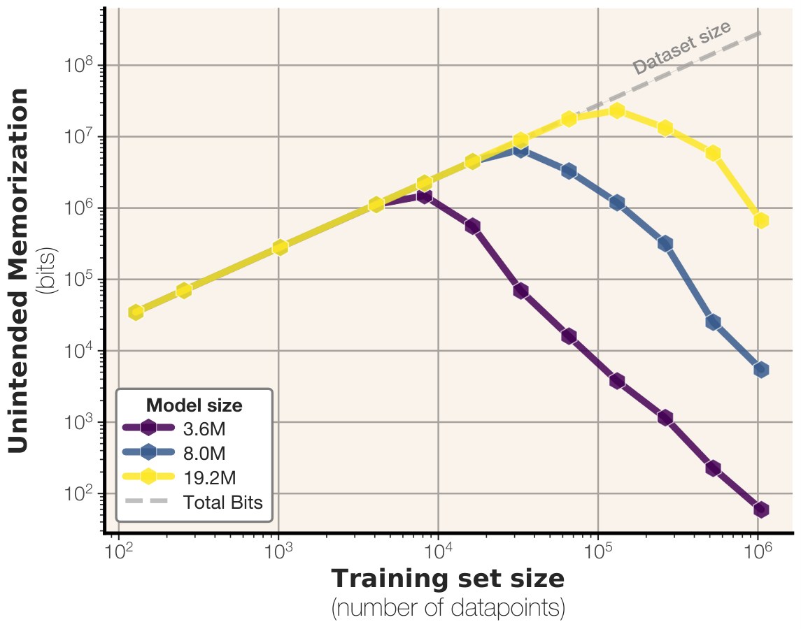
Figure 2: Unintended memorization of text across model and dataset sizes (Section 4). All quantities are calculated with respect to a large oracle model trained on the full data distribution.
图 2:不同模型规模与数据集规模下,文本上的非预期记忆(第 4 节)。所有量都相对于在完整数据分布上训练的大型 oracle 模型计算。
1 Introduction
1 引言
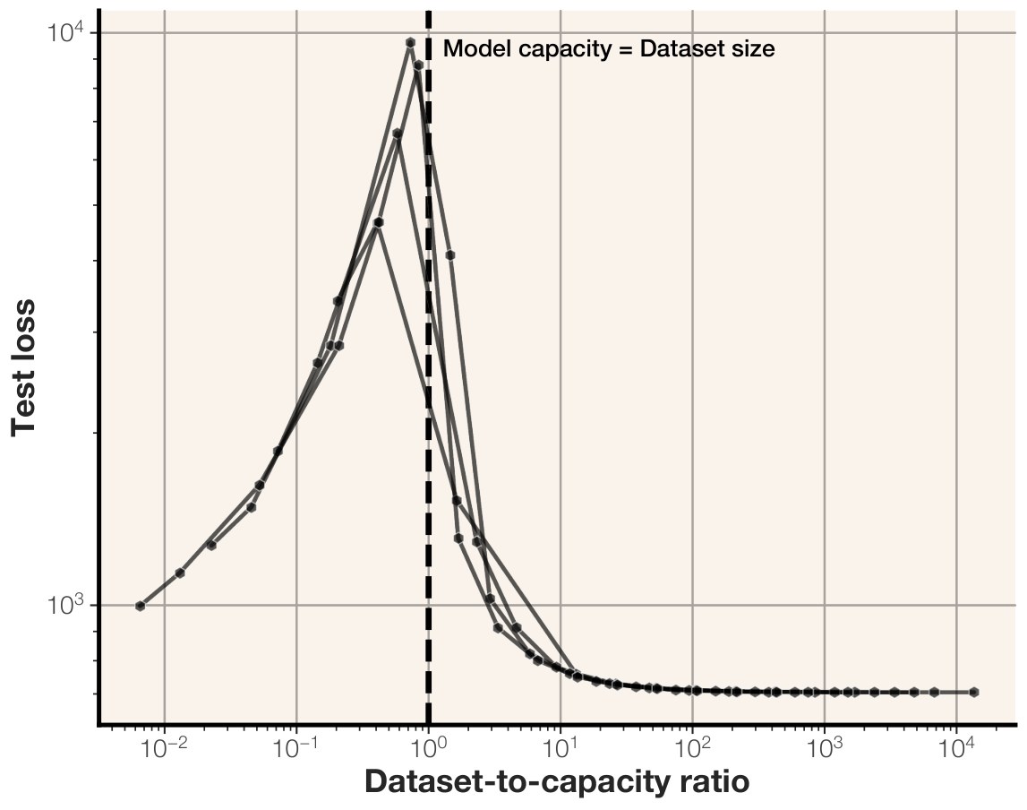
Figure 3: In our experiments on synthetic bitstrings, double descent occurs exactly when the dataset size begins to exceed the model’s capacity, when unintended memorization is no longer beneficial for lowering the loss.
图 3:在合成比特串实验中,双重下降恰好出现在数据集规模开始超过模型容量之时,也就是非预期记忆不再有助于降低损失的时候。
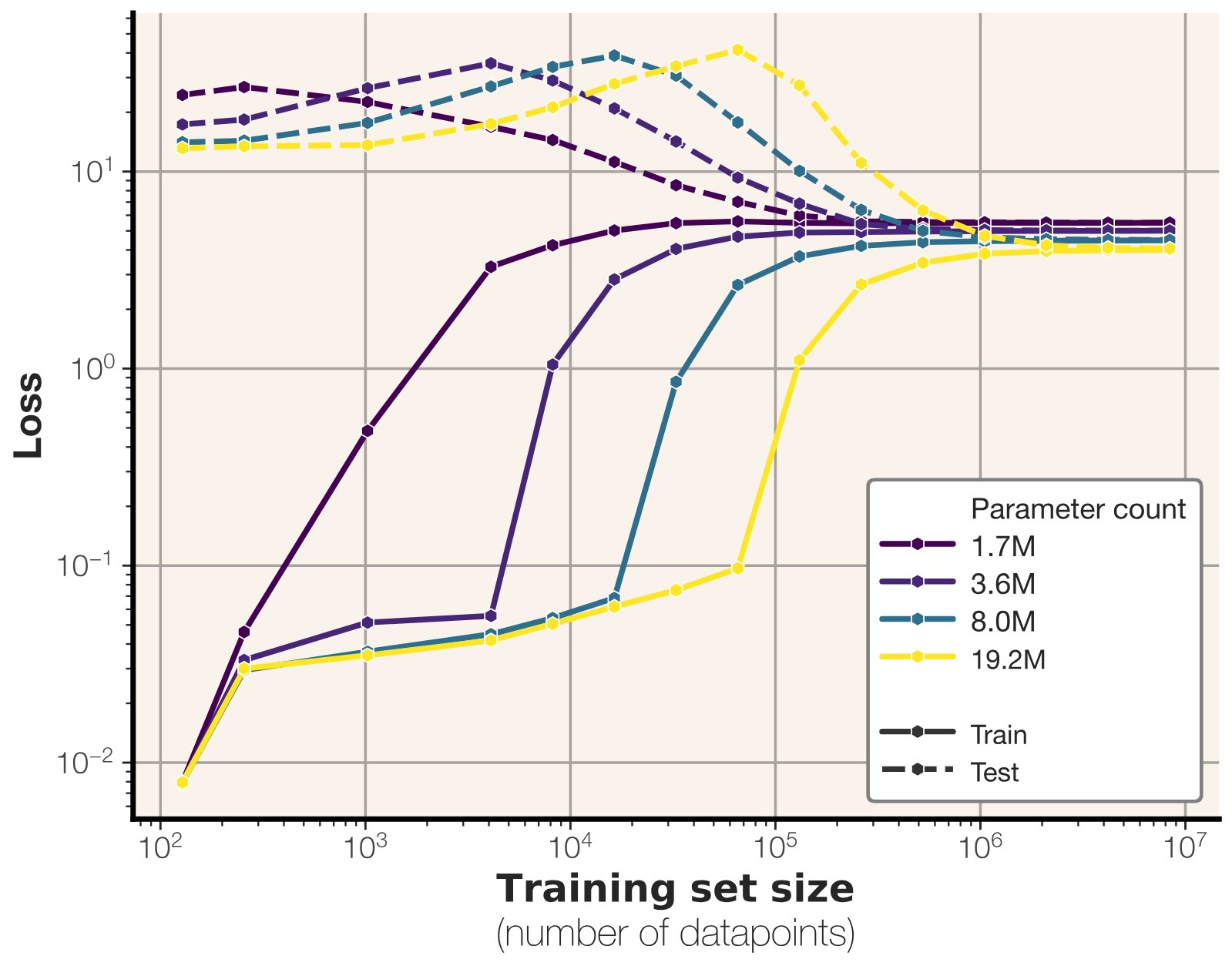
Figure 4: Train and test losses of different model and dataset sizes trained on text. Double descent occurs when dataset size exceeds model capacity.
图 4:在文本上训练的不同模型规模与数据集规模的训练损失和测试损失。当数据集规模超过模型容量时出现双重下降。
For the past several years, modern language models have been trained on increasingly large amounts of data, while parameter counts stay stagnant in the billions. For example, one recent state-of-the-art model (Dubey & et al, 2024) has 8 billion parameters (around on disk) but is trained on 15 trillion tokens (around on disk).
过去几年里,现代语言模型用的数据量越来越大,参数量却仍停留在数十亿的量级。例如,最近一个先进模型(Dubey & et al, 2024)有 80 亿参数(磁盘上大约 ),却在 15 万亿 token(磁盘上大约 )上训练。
A long line of work (Carlini et al., 2019; Mireshghallah et al., 2022; Nasr et al., 2023; Zhang et al., 2023; Carlini et al., 2023b; Schwarzschild et al., 2024) questions whether such pretrained language models memorize their training data in a meaningful way. Most research approaches this problem either through the lens of extraction, aiming to recover full training datapoints from model weights, or membership inference, classifying whether a training point was present in the training data of a given model.
一系列工作(Carlini et al., 2019; Mireshghallah et al., 2022; Nasr et al., 2023; Zhang et al., 2023; Carlini et al., 2023b; Schwarzschild et al., 2024)追问:这类预训练语言模型是否以有意义的方式记住了训练数据。多数研究从两个角度切入:一是抽取,试图从模型权重中恢复完整的训练样本;二是成员推断,判断某条样本是否出现在给定模型的训练集里。
Studies of language model extraction argue that a datapoint is memorized if we can induce the model to generate it (Carlini et al., 2023b; Nasr et al., 2023; Schwarzschild et al., 2024). We argue that such generation does not necessarily serve as a proof of memorization. Language models can be coerced to output almost any string (Geiping et al., 2024); hence the fact that a model outputs something is not necessarily a sign of memorization. To address this issue, some researchers have suggested regularizing the input to the language model, such as by limiting its length (Schwarzschild et al., 2024) or matching it to the prefix (Carlini et al., 2023b) preceding the memorized sentence. However, none of these constraints allow us to distinguish whether a model outputs a string due to memorization or good generalization. For example, a language model prompted to add two numbers can output the answer without having seen the equation before.
语言模型抽取方面的研究认为,如果我们能诱使模型生成某条样本,这条样本就算被记住了(Carlini et al., 2023b; Nasr et al., 2023; Schwarzschild et al., 2024)。我们则认为,能够生成并不必然构成记忆的证据。语言模型几乎可以被诱导输出任意字符串(Geiping et al., 2024);因此,模型输出了某段文字,并不一定说明它记住了这段文字。为处理这一点,有研究者建议约束语言模型的输入,例如限制长度(Schwarzschild et al., 2024),或把输入限制为被记句子前面的前缀(Carlini et al., 2023b)。但这些约束都无法区分:模型输出某串文字,究竟是因为记住了它,还是因为泛化得好。例如,提示语言模型做两个数的加法,它可以给出答案,即使从未见过这道算式。
To address this issue, we propose a definition of memorization that quantifies the extent to which a model retains information about a specific datapoint. Our approach leverages the concept of compression rate in bits: a model is considered to have memorized an input if the input can be compressed into a shorter encoding when the model is available. This framework draws inspiration from Kolmogorov information theory (Kolmogorov, 1963) and Shannon information theory (Shannon, 1948), but remains practical by estimating information content using model likelihoods. We address the fundamental challenge of distinguishing memorization from generalization (Prashanth et al., 2024) by decomposing memorization into two distinct components: unintended memorization, which captures the information the model retains about a specific dataset, and generalization, which represents the knowledge the model acquires about the underlying data-generating process. This separation is similar to the approach in (Brown et al., 2021), which defines memorization using conditional mutual information between the dataset and the trained model, conditioned on the true concept. However, our notion differs in that it enables this separation at the instance level using algorithmic definitions of information.
为此,我们提出一种记忆定义,用来量化模型对某条具体样本保留了多少信息。方法借助以比特计的压缩率:如果在有模型可用时,输入能被压成更短的编码,就认为模型记住了这个输入。这一框架从 Kolmogorov 信息论(Kolmogorov, 1963)和 Shannon 信息论(Shannon, 1948)获得启发,同时保持可操作,用模型似然来估计信息量。要把记忆与泛化区分开(Prashanth et al., 2024),我们把记忆拆成两个不同部分:非预期记忆刻画模型对某个具体数据集保留的信息,泛化则表示模型关于底层数据生成过程学到的知识。这种分离接近 Brown et al. (2021) 的做法,他们用数据集与训练所得模型在真实概念条件下的条件互信息来定义记忆。我们的定义不同之处在于,它借助算法信息的定义,能在实例层面做这种分离。
To understand our new quantities, we measure unintended memorization and generalization by training language models of varying capacity on datasets of different sizes. We first eliminate the question of generalization entirely by training on a dataset of random uniformly-sampled bitstrings. In this setting, we can exactly measure the amount of information contained about the data inside the model. This gives us a principled way to measure language model capacity when trained on uniform datasets of exact known information content. We find that GPT-style transformers can store between 3.5 and 4 bits of information in each model parameter, depending on model architecture and precision.
为理解这些新的量,我们在不同容量的语言模型、不同规模的数据集上测量非预期记忆和泛化。我们先彻底去掉泛化问题,在均匀随机采样的比特串数据集上训练。在这种设定下,可以精确测量模型里存了多少关于数据的信息。当训练数据是信息量精确已知的均匀数据集时,这就给出了一种有原则地测量语言模型容量的方法。我们发现,按架构和精度不同,GPT 风格 Transformer 可以在每个模型参数中存储 3.5 到 4 比特的信息。
We then repeat our experiments with real text, where generalization is possible and even beneficial for learning. On real text, language models memorize up to a certain capacity, at which point they substitute unintended memorization for generalization, and begin to learn general, reusable patterns as opposed to sample-level specifics. Our framework shows that double descent phenomenon begins to occur at this point, when the data size exceeds the model capacity in bits.
随后我们把实验改到真实文本上,这时泛化是可能的,甚至对学习有益。在真实文本上,语言模型会记忆到某一容量为止;此后它们用泛化替代非预期记忆,开始学习可复用的一般模式,而不是样本级的细节。我们的框架表明,双重下降现象正是在这一点开始出现,也就是数据规模(以比特计)超过模型容量的时候。
Finally, we use our results to predict a scaling law for membership inference performance based on model capacity and dataset size. We show that membership inference follows a clean relationship based on model capacity and dataset size: bigger models can memorize more samples, and making datasets bigger makes membership inference harder. Our scaling laws extrapolate to larger models, and predict most modern language models are trained on too much data to do reliable membership inference on the average datapoint.
最后,我们用这些结果预测一条由模型容量和数据集规模决定的成员推断性能缩放律。结果表明,成员推断与模型容量、数据集规模之间有清晰关系:更大的模型能记住更多样本,把数据集做大则使成员推断更难。这些缩放律可以外推到更大的模型,并预测:多数现代语言模型用的数据太多,因而无法对平均样本做可靠的成员推断。
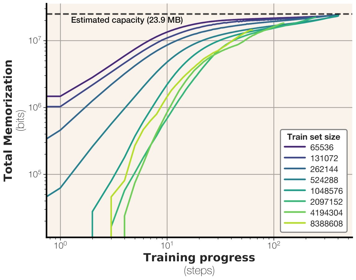
Figure 5: Bits memorized across training. This particular model is a GPT-style transformer with parameters and a capacity of MB.
图 5:训练过程中记住的比特数。这个模型是 GPT 风格 Transformer,有 个参数,容量为 MB。
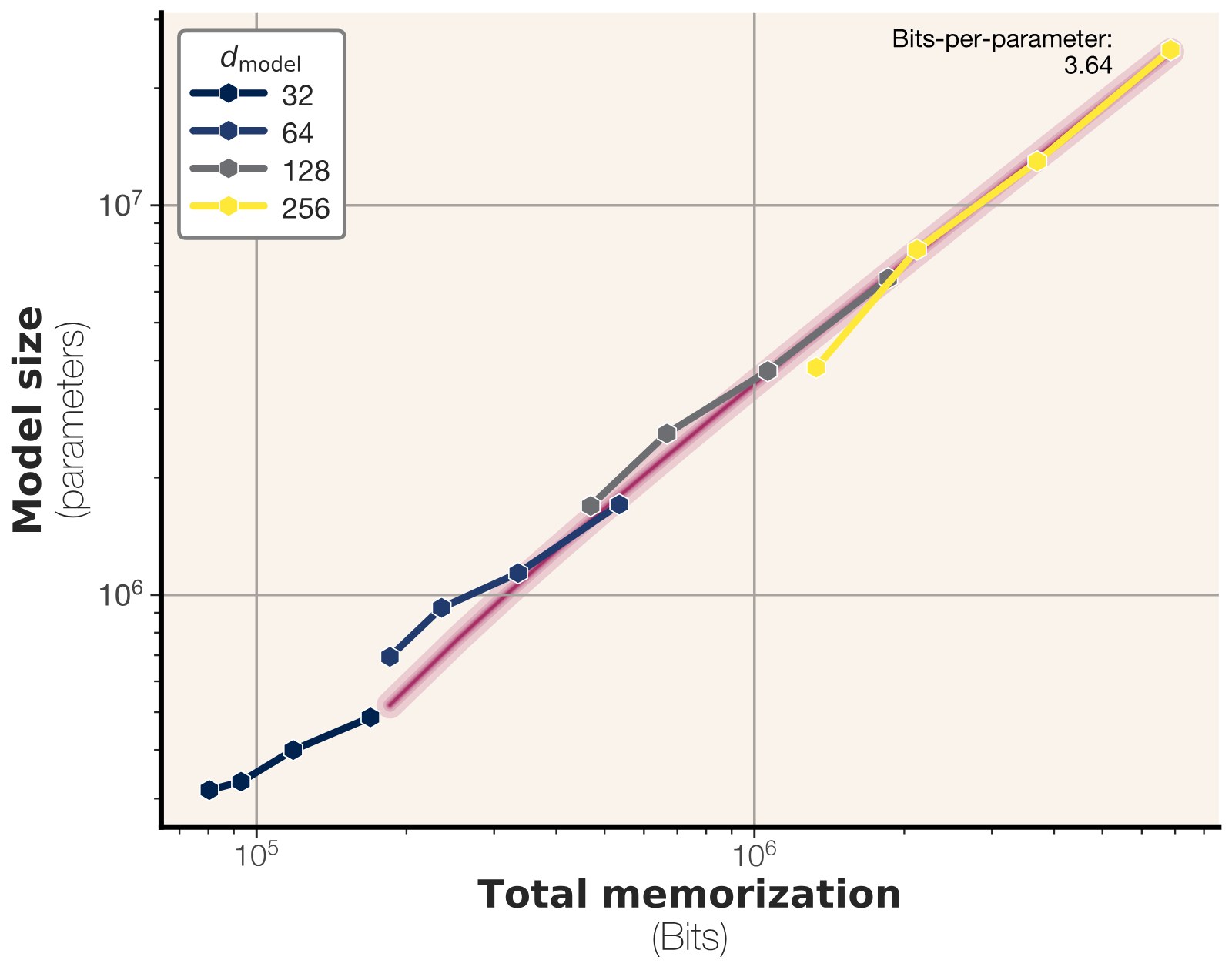
Figure 6: Capacity in bits-per-parameter for models trained on synthetic data. We estimate bits-per-parameter for GPT models trained in half precision.
图 6:在合成数据上训练的模型以每参数比特计的容量。对半精度训练的 GPT 模型,我们估计 比特/参数。
2 Memorization, intended and unintended
2 记忆:预期的与非预期的
When a model is trained using a training algorithm and a dataset , some information is transferred from the sample to the model . A key question in the memorization literature is determining how much of this stored information is intended versus unintended. In this work, we aim to provide a rigorous definition of memorization that satisfies certain properties:
当模型 由训练算法 在数据集 上训练时,一部分信息会从样本 传到模型 。记忆文献里的一个关键问题是:这些被存储的信息里,有多少是预期的,有多少是非预期的。本文希望给出一个满足若干性质的严格记忆定义:
- Separation from generalization. Our notion of unintended memorization must be distinct from intended memorization, which we refer to as generalization. For example, consider a language model trained on the sample: Q: What is ? A: 1267650600228229401496703205376. When assessing how much of this training sample is memorized, we must account for the fact that performing simple math operations is expected from a language model.
- 与泛化分离。 非预期记忆必须不同于预期记忆,后者我们称为泛化。例如,设语言模型在这样一条样本上训练:Q: What is ? A: 1267650600228229401496703205376. 评估这条训练样本被记住了多少时,必须考虑到:完成简单数学运算,本来就是对语言模型的预期。
- Sample-level memorization. We need to define memorization for realizations of random variables, not the random variables themselves. Specifically, we want to determine how much unintended memorization of a sample occurs in a model .
- 样本级记忆。 我们需要针对随机变量的实现来定义记忆,而不是针对随机变量本身。具体来说,我们想确定:模型 对样本 发生了多少非预期记忆。
- Independence from training algorithm. Our definition should be independent of the training algorithm and only a function of the final model and the sample . This is crucial for language models, where we often only have access to the final model and target sample.
- 与训练算法无关。 定义应当不依赖于训练算法 ,而只是最终模型 与样本 的函数。这对语言模型很重要,因为我们往往只能拿到最终模型和目标样本。
Previous works have attempted to define memorization for machine learning models. We aim to provide precise definitions of memorization that meet our criteria, and offer ways to measure it. See Appendix B for a broader discussion on definitions of memorization.
已有工作试图为机器学习模型定义记忆。我们希望给出满足上述条件的精确定义,并提供测量方法。关于记忆定义的更广泛讨论见附录 B。
2.1 Warm-up: A statistical view of memorization
2.1 热身:记忆的统计视角
Notation. In this section, we use capital letters (e.g. , ) to refer to random variables and lowercase letters to refer to instances of a random variable (e.g. and ).
记号。 本节用大写字母(如 、)表示随机变量,用小写字母表示随机变量的实例(如 和 )。
We rely on information theory, which has developed well-understood notions of information for random variables. For a random variable , we use , the entropy of , to define the amount of information present in . For two distinct random variables , we can define as the uncertainty left in after fixing . With these definitions, we can now measure mutual information between and by subtracting the leftover information from the total information: .
我们借助信息论,它为随机变量提供了成熟的信息概念。对随机变量 ,用 的熵 表示 中的信息量。对两个不同的随机变量 ,可以把 定义为固定 之后 中剩余的不确定性。有了这些定义,就可以用总信息减去剩余信息,来测量 与 之间的互信息:。
Now suppose we have a machine learning pipeline. We have a prior on the underlying model that captures our dataset distribution , and a learning algorithm that maps samples from to a trained model . To understand how much information about is stored in , we can use the notion of mutual information:
现在考虑一条机器学习流水线。我们对刻画数据集分布 的底层模型有先验 ,并有学习算法 ,把来自 的样本映射为训练后的模型 。要理解 里存了多少关于 的信息,可以用互信息:
Note that this captures all the information about that is stored in . As we discussed, we need our notion of memorization to account for generalization as well. So when measuring unintended memorization, we are only interested in the information that is present in , which is the uncertainty left in after fixing . Hence, we can define unintended memorization as
注意,这捕获了存储在 中的全部关于 的信息。如前所述,记忆的概念还需要把泛化考虑进去。因此,在测量非预期记忆时,我们只关心 中的信息,也就是固定 之后 里剩下的不确定性。于是可以把非预期记忆定义为
and then the generalization (or intended memorization) must be
于是,泛化(或称预期记忆)就是
having defined our notions of intended and unintended memorization we turn our attention to practically measuring them. Let us first state a proposition that enables measurement of unintended memorization:
在定义了预期记忆与非预期记忆之后,我们转向如何在实践中测量它们。先陈述一条命题,它使我们能够测量非预期记忆:
Proposition 1(Super-additivity of Unintended Memorization).
命题 1(非预期记忆的超可加性)。
Assume is a dataset of i.i.d. samples. We have
设 是由 个独立同分布样本组成的数据集。我们有
This proposition shows that to measure a lower bound on the unintended memorization on the dataset level, we can sum per-sample memorization. On the other hand, the entropy of the information content of the trained model itself servers as an upper bound on the unintended memorization. Another implication of this implies that unintended memorization should scale with the dataset size but cannot exceed the total capacity of the model.
这条命题表明,要在数据集层面给出非预期记忆的下界,可以把各条样本的记忆量加起来。另一方面,训练所得模型自身信息量的熵,构成非预期记忆的上界。由此还可得到:非预期记忆应随数据集规模增大,但不能超过模型的总容量。
We note that this statistical definition of memorization was first introduced by Brown et al. (2021), where they theoretically looked at the role of unintended memorization in enabling successful learning for certain tasks. However, this preliminary definition is unsuitable for us as we aim to practically measure instance-level memorization. In particular, since we observe only a single trained model and a single input sample, we are unable to define probabilities or conditional probabilities over samples conditioned on the model.
我们指出,这种记忆的统计定义最早由 Brown et al. (2021) 提出,他们从理论上考察了非预期记忆在某些任务上促成成功学习所起的作用。不过,这个初步定义对我们并不合适,因为我们希望实际测量实例级记忆。特别是,我们只能观察到一个训练好的模型和一条输入样本,因而无法定义概率,也无法定义以模型为条件的样本条件概率。
2.2 Measuring unintended memorization with Kolmogorov Complexity
2.2 用 Kolmogorov 复杂度测量非预期记忆
Our definitions of memorization and generalization so far are defined using an “entropy-based” notion of information. This means our definitions can only be used for random variables. This brings big challenges in measuring memorization. All our variables in the definition of memorization are singletons. We have a single underlying model , we have a single dataset and we have a single trained model [^1]. It is impossible to measure the entropy (let alone conditional entropy) of the underlying variables using a single sample.
到目前为止,记忆和泛化的定义都建立在「基于熵」的信息概念上。这意味着这些定义只能用于随机变量。这给测量记忆带来很大困难。定义里出现的变量全都是单例:我们有一个底层模型 ,有一个数据集 ,还有一个训练好的模型 [^1]。只用一个样本,不可能测量这些底层变量的熵(更不用说条件熵)。
To this end, we switch to another notion of information based on compression, then later we show how this notion closely approximates the notion of memorization defined above. Kolmogorov complexity defines the information content of a string , denoted as , to be the length of shortest representation of in a given computational model. Similarly, we can define the leftover information , to be the shortest representation of , when we have available as a reference. And the information content of , denoted by , is the length of such description. Then, we can define mutual information in a similar fashion:
为此,我们改用另一种基于压缩的信息概念,稍后再说明它如何密切近似上面定义的记忆。Kolmogorov 复杂度把字符串 的信息量记为 ,定义为在给定计算模型下 的最短表示的长度。类似地,可以把剩余信息 定义为:在 可作为参照时, 的最短表示;而 的信息量记为 ,就是这一描述的长度。然后可以用类似方式定义互信息:
Definition 2(Kolmogorov complexity).
定义 2(Kolmogorov 复杂度)。
Let be an arbitrary computational model that takes a set of inputs and returns an output (e.g. universal Turing machine). The shortest description of with respect to computational model is defined as Also, the Kolmogorov complexity of relative to another string is defined as And we define the Kolmogorov mutual information between and by We assume inputs are bitstrings and is the bit length of the input.
设 是任意一个计算模型,它接受一组输入并返回输出(例如通用图灵机)。相对于计算模型 , 的最短描述定义为 。此外, 相对于另一字符串 的 Kolmogorov 复杂度定义为 。我们把 与 之间的 Kolmogorov 互信息定义为 。假设输入是比特串, 是输入的比特长度。
Definition 3(Kolmogorov memorization).
定义 3(Kolmogorov 记忆)。
Let be a reference model that approximates the true distribution of data, and be a model trained on a dataset . For each we define the memorization of in as We also define intended and unintended variants of memorization:
设 是近似真实数据分布的参照模型, 是在数据集 上训练得到的模型。对每个 ,我们把 在 中的记忆定义为 。我们也定义记忆的预期与非预期变体:
There are known connections between Kolmogorov complexity and Shannon Entropy (Grunwald & Vitanyi, 2004). These results point at the conceptual connection between the two notions and imply that . Interestingly, this implies that our notion of Kolmogorov memorization closely approximates Shannon memorization.
Kolmogorov 复杂度与 Shannon 熵之间已有已知联系(Grunwald & Vitanyi, 2004)。这些结果指出两种概念在思想上的关联,并意味着 。有意思的是,这说明我们的 Kolmogorov 记忆概念能够密切近似 Shannon 记忆。
Proposition 4.
命题 4。
Let be an i.i.d, dataset distribution parametrized by ground-truth model . Let be a training algorithm mapping to . Assume and [^2]. Then we have for some constant independent of and .
设 是由真实模型 参数化的独立同分布数据集分布。设 是把 映射到 的训练算法。假设 且 [^2]。则有 ,其中常数 与 和 无关。
2.3 Estimating Kolmogorov with compression
2.3 用压缩估计 Kolmogorov 复杂度
Fixing our notion of Kolmogorov memorization, we now describe how we can estimate in different setups. Note that exact calculation of Kolmogorov complexity is known to be uncomputable (Kolmogorov, 1965). However, we can still approximate it using the best available compression schemes. These compression schemes could be arbitrary algorithms, e.g. using prompt optimization as in Schwarzschild et al. (2024) or using text prefixes as in Carlini et al. (2023b).
在确定了 Kolmogorov 记忆的概念之后,我们说明如何在不同设定下估计 。需要指出,精确计算 Kolmogorov 复杂度是不可计算的(Kolmogorov, 1965)。但我们仍可用现有最好的压缩方案来近似。这些压缩方案可以是任意算法,例如 Schwarzschild et al. (2024) 的提示优化,或 Carlini et al. (2023b) 使用文本前缀的做法。
We adopt arithmetic coding as the most natural compression algorithm for language. Arithmetic coding is not only effective for text compression Delétang et al. (2024), but it also allows code lengths to be computed efficiently using model likelihoods. A promising direction for future research is to design compression algorithms specifically tailored to minimize the code length of training data in machine learning models and use it to obtain more accurate estimation of Kolmogorov complexity and memorization. Below, we summarize how we approximate each term in our memorization definition using model likelihoods.
对语言而言,我们采用算术编码作为最自然的压缩算法。算术编码不仅对文本压缩有效(Delétang et al., 2024),还能借助模型似然高效计算码长。一个有前景的后续方向,是专门设计用于缩短机器学习模型中训练数据码长的压缩算法,并用它更准确地估计 Kolmogorov 复杂度和记忆。下面我们概括如何用模型似然来近似记忆定义中的各项。
- : Here, is the trained target model, which does not necessarily capture the true data distribution. We do not really calculate the compressed code, instead we use fact that the compression rate of arithmetic coding tied to the likelihood of the model (Shannon, 1950). So, we can estimate by the negative log likelihood of under the target model, .
- :这里 是训练得到的目标模型,它不一定刻画真实数据分布。我们并不真正算出压缩码,而是利用算术编码的压缩率与模型似然相联系这一事实(Shannon, 1950)。因此,可以用目标模型下 的负对数似然 来估计 。
- : In this case, the compression algorithm has access to both target and reference models. We simply compute . In practice, our choice of reference model is a larger model with the same architecture as trained for many steps on a much wider data distribution.
- :这时压缩算法同时可以使用目标模型和参照模型。我们直接计算 。实践中,我们选择的参照模型是与 同结构的更大模型,并在宽得多的数据分布上训练很多步。
A curious reader may notice that we began with a likelihood-based notion of memorization, then shifted to a definition grounded in Kolmogorov complexity, and ultimately returned to likelihood to estimate that complexity. We emphasize, however, that the likelihood used in our approximation of Kolmogorov memorization is distinct from the initial likelihood notion. In particular, this likelihood is dependent on the parameters of the decoding algorithm, such as temperature or top-k sampling. More broadly, we note that any compression algorithm can be used to approximate Kolmogorov complexity, and our choice of arithmetic coding is just one instantiation of this broader framework.
细心的读者可能会注意到:我们从基于似然的记忆概念出发,转到以 Kolmogorov 复杂度为基础的定义,最后又回到似然来估计这一复杂度。但需要强调,用来近似 Kolmogorov 记忆的似然,不同于一开始那个似然概念。特别是,这里的似然依赖于解码算法的参数,例如温度或 top-k 采样。更一般地说,任何压缩算法都可以用来近似 Kolmogorov 复杂度,采用算术编码只是这一更广框架中的一种具体实现。
Choice of reference model.
参照模型的选择。
In this work we use two reference models to compute . In our experiments on synthetic random strings (Section 3) we know the exact underlying data distribution and use that as a reference model. In our experiments on text (Section 4) we select to be a large model of the same family, trained on a much larger superset of the training data for .
本文用两个参照模型来计算 。在合成随机字符串实验(第 3 节)中,我们恰好知道底层数据分布,并把它当作参照模型。在文本实验(第 4 节)中,我们把 选为同一系列的更大模型,它在 训练数据的一个大得多的超集上训练。
| [bits] | [bpp] | |||||
|---|---|---|---|---|---|---|
| Params | fp32 | bf16 | fp32 | bf16 | ||
| 1 | 32 | 8.04 | 3.39 | 3.16 | 4.23 | 3.93 |
| 64 | 1.85 | 7.27 | 6.93 | 3.92 | 3.74 | |
| 128 | 4.69 | 1.71 | 1.69 | 3.65 | 3.61 | |
| 256 | 1.33 | 4.15 | 3.83 | 3.12 | 2.88 | |
| 2 | 32 | 9.31 | 3.87 | 3.31 | 4.16 | 3.56 |
| 64 | 2.35 | 9.60 | 9.27 | 4.08 | 3.94 | |
| 128 | 6.67 | 2.66 | 2.60 | 3.99 | 3.89 | |
| 256 | 2.12 | 8.49 | 7.76 | 4.01 | 3.66 | |
| 4 | 32 | 1.18 | 4.65 | 3.99 | 3.92 | 3.37 |
| 64 | 3.35 | 1.34 | 1.14 | 3.98 | 3.39 | |
| 128 | 1.06 | 4.02 | 3.75 | 3.78 | 3.53 | |
| 256 | 3.70 | 1.36 | 1.30 | 3.68 | 3.51 | |
| 8 | 32 | 1.69 | 5.12 | 4.85 | 3.02 | 2.86 |
| 64 | 5.35 | 2.05 | 1.71 | 3.83 | 3.19 | |
| 128 | 1.86 | 7.23 | 6.49 | 3.89 | 3.49 | |
| 256 | 6.86 | 2.71 | 2.51 | 3.96 | 3.65 | |
| Mean (): | ||||||
| 3.83 | 3.51 |
Table 1: Model capacity estimates across different widths and depths in full and half-precision. Doubling precision from bfloat16 to float32 only increases model capacity from to bits-per-parameter.
| [比特] | [bpp] | |||||
|---|---|---|---|---|---|---|
| 参数量 | fp32 | bf16 | fp32 | bf16 | ||
| 1 | 32 | 8.04 | 3.39 | 3.16 | 4.23 | 3.93 |
| 64 | 1.85 | 7.27 | 6.93 | 3.92 | 3.74 | |
| 128 | 4.69 | 1.71 | 1.69 | 3.65 | 3.61 | |
| 256 | 1.33 | 4.15 | 3.83 | 3.12 | 2.88 | |
| 2 | 32 | 9.31 | 3.87 | 3.31 | 4.16 | 3.56 |
| 64 | 2.35 | 9.60 | 9.27 | 4.08 | 3.94 | |
| 128 | 6.67 | 2.66 | 2.60 | 3.99 | 3.89 | |
| 256 | 2.12 | 8.49 | 7.76 | 4.01 | 3.66 | |
| 4 | 32 | 1.18 | 4.65 | 3.99 | 3.92 | 3.37 |
| 64 | 3.35 | 1.34 | 1.14 | 3.98 | 3.39 | |
| 128 | 1.06 | 4.02 | 3.75 | 3.78 | 3.53 | |
| 256 | 3.70 | 1.36 | 1.30 | 3.68 | 3.51 | |
| 8 | 32 | 1.69 | 5.12 | 4.85 | 3.02 | 2.86 |
| 64 | 5.35 | 2.05 | 1.71 | 3.83 | 3.19 | |
| 128 | 1.86 | 7.23 | 6.49 | 3.89 | 3.49 | |
| 256 | 6.86 | 2.71 | 2.51 | 3.96 | 3.65 | |
| 均值 (): | ||||||
| 3.83 | 3.51 |
表 1:不同宽度与深度下、全精度与半精度的模型容量估计。把精度从 bfloat16 提高到 float32,模型容量只从每参数 比特增加到 比特。
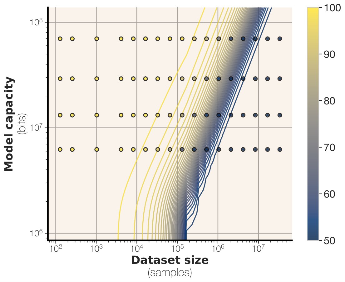
Figure 7: Scaling law curves for membership inference overlaid with empirical data, shown in circles.
图 7:成员推断的缩放律曲线,叠加以圆点表示的经验数据。
3 Model Capacity for Memorization
3 用于记忆的模型容量
Unintended memorization provides us a principled way of measuring the precise number of bits a model knows about a datapoint . If we add up the information for each datapoint in a dataset, we can measure the total amount of bits a model knows about the dataset. And in cases where generalization is not possible because each datapoint is completely independent, we can estimate the capacity of a given model by summing per-datapoint unintended memorization.
非预期记忆提供了一种有原则的方法,用来精确测量模型 对数据点 知道多少比特。如果把数据集中每个数据点的信息加起来,就可以测量模型对整个数据集知道的总比特数。在各条数据完全独立、因而无法泛化的情形下,把逐条非预期记忆求和,就可以估计给定模型 的容量。
3.1 Defining model capacity
3.1 定义模型容量
We first formalize this notion of memorization capacity for a particular language model . Capacity is the total amount of memorization that can be stored in across all its parameters.
我们先把记忆容量的概念形式化,针对某个具体的语言模型 。容量是 可以在其全部参数中存储的记忆总量。
Definition 5(Capacity).
定义 5(容量)。
Let be a distribution and a learning algorithm. We define the capacity of the learning algorithm to be
设 是一个分布, 是学习算法。我们把学习算法 的容量定义为
When the model capacity is reached, will no longer increase with dataset size. In practice, we can compute capacity by training to saturation on varying sizes of and computing the maximum memorization.
一旦达到模型容量, 便不再随数据集规模增大。实践中,可以在不同规模的 上训练至饱和,再取记忆量的最大值来计算容量。
3.2 Measuring model capacity with synthetic sequences
3.2 用合成序列测量模型容量
In this section we measure the capacity of Transformer language models. Our goal is to instantiate multiple datasets and distributions and measure the memorization of them when training a single model . Then, we take the maximum over all datasets to approximate of the model’s capacity. For instantiating our datasets, each token is uniformly sampled from a predefined set of tokens independent of the previous tokens.
本节测量 Transformer 语言模型的容量。目标是构造多个数据集和分布,在训练同一个模型 时测量对它们的记忆,再对所有数据集取最大值,以近似模型容量。构造数据集时,每个 token 都从预先给定的词表中均匀采样,且与前面的 token 独立。
To approximate , we can directly compute entropy under the trained model to calculate the shortest description of the dataset conditioning on . Subtracting the two, we can approximate the unintended memorization . Since the process for sampling the data is completely random, there is no generalization to be stored within (that is, ).
为近似 ,我们可以直接计算训练后模型下的熵,从而得到以 为条件时数据集的最短描述。两者相减,即可近似非预期记忆 。由于数据的采样过程完全随机, 中没有可存储的泛化(也就是 )。
Observe that when we sample synthetic sequences from a uniform distribution, we can compute their Shannon information exactly. Given a dataset size , we construct a dataset of sequences, each of tokens. Given a vocabulary size , we can calculate the total entropy of a dataset with such parameters by . Then we calculate the compressed form using entropy under to compute the code length and use this as an approximation of . Then we calculate the and compute a model’s capacity as the maximum amount of memorization over all datasets.
注意到,当合成序列从均匀分布中采样时,它们的 Shannon 信息可以精确计算。给定数据集规模 ,我们构造由 条序列组成的数据集,每条有 个 token。给定词表大小 ,具有这些参数的数据集 的总熵为 。然后用 下的熵计算 的压缩形式,得到码长,并把它作为 的近似。再计算 ,并把模型容量取为在所有数据集上记忆量的最大值。
Experimental details.
实验细节。
In accordance with Kaplan et al. (2020), we train models with the GPT-2 architecture (Radford et al., 2019) initialized from scratch. Our models have between and layers, hidden dimensions scaled from to , and from to parameters. We train models for steps with a batch size of . We use the Adam optimizer. All models are trained on a single A100 GPU in bfloat16 precision, and we use gradient accumulation if a batch cannot fit in memory. Unless otherwise noted, we set vocabulary size , sequence length and vary only the number of points in a dataset. We train each model on each dataset size over five random seeds, which affect both model initialization and the dataset sampling.
依照 Kaplan et al. (2020),我们从零初始化训练 GPT-2 架构(Radford et al., 2019)的模型。模型有 到 层,隐藏维从 到 ,参数量从 到 。训练 步,批量大小为 ,优化器为 Adam。所有模型都在单块 A100 GPU 上以 bfloat16 精度训练;若一个批次无法放入显存,则使用梯度累积。除非另有说明,词表大小取 ,序列长度取 ,只改变数据集中的样本数。每个模型在每个数据集规模上用五个随机种子训练,种子同时影响模型初始化和数据集采样。
Results.
结果。
We plot memorization across model and data sizes in Figure 2. This allows us to visualize unintended memorization amounts (y-axis) across dataset sizes (x-axis) grouped by model size (line color). We observe a striking plateau once a model reaches its capacity. Given the dataset is large enough, models exhibit an upper bound in net memorization, regardless of data size. Small datasets are completely memorized by all models with enough capacity.
我们在图 2 中画出不同模型规模与数据规模下的记忆量。这样可以按模型规模(线条颜色)分组,观察非预期记忆量(纵轴)如何随数据集规模(横轴)变化。一旦模型达到其容量,会出现非常明显的平台。只要数据集足够大,无论数据再增大,模型的净记忆量都有一个上界。规模较小的数据集则会被所有容量足够的模型完整记住。
We estimate the capacity of each model as the maximum amount of unintended memorization in bits measured across all dataset sizes. We then compare this capacity to the model size in Figure 6. Interestingly, even at this small scale, we see a very smooth relationship between observed capacity (maximum memorization measured over all datasets) and model parameters. We plot this relationship in Figure 6: under these settings, our models consistently memorize between and bits per parameter. This corroborates the findings of prior work such as (Roberts et al., 2020; Lu et al., 2024), which noticed that fact storage scales linearly with model capacity. Ours is a slightly larger estimate than Allen-Zhu & Li (2024), which estimated via quantization that models can store around bits per parameter.
我们把每个模型的容量估计为:在所有数据集规模上测得的非预期记忆比特数的最大值。然后在图 6 中把这一容量与模型规模比较。有意思的是,即便在这一较小尺度上,观测到的容量(所有数据集上测得的最大记忆量)与模型参数量之间已有非常平滑的关系。我们把这一关系画在图 6 中:在这些设定下,模型稳定地记住每参数 到 比特。这与先前工作(Roberts et al., 2020; Lu et al., 2024)的发现相一致,那些工作注意到事实存储随模型容量线性增长。我们的估计略高于 Allen-Zhu & Li (2024),他们通过量化估计模型大约能存储每参数 比特。
Since our models are learned via gradient descent, they are not guaranteed to find the global optima; thus, we are only ever measuring a lower bound on model capacity. We take a closer look at the training curves to analyze the convergence of our 8M parameter language model. We plot model convergence throughout training in Figure 6.
由于模型是用梯度下降学习的,并不保证找到全局最优;因此我们测量的始终只是模型容量的下界。我们更仔细地查看训练曲线,分析这个 800 万参数语言模型的收敛情况,并在图 6 中画出整个训练过程中的收敛。
In this case, all datasets from 16,000 to 4M samples fall within a range of bits memorized. This indicates that our measurements are robust within an order of magnitude, and we do not expect to memorize significantly more information by training for more steps. This finding also confirms our hypothesis that capacity scales roughly with parameter count. The two largest datasets (4M and 8M samples, respectively) converge to total memorization of and bits memorized. We expect that their memorization rates would continue to increase toward the capacity had we trained for more epochs.
在这种情形下,从 16,000 到 400 万条样本的所有数据集,记住的比特数都落在 的范围内。这表明我们的测量在一个数量级内是稳健的,并且不预期再训练更多步会记住显著更多的信息。这一发现也印证了我们的假设:容量大致随参数量缩放。两个最大的数据集(分别为 400 万和 800 万条样本)收敛到的总记忆量为 和 比特。我们预期,若训练更多轮,它们的记忆率还会继续升向容量。
How does precision affect capacity?
精度如何影响容量?
One natural question is how our estimates for depend on the precision of language model training. In fact, although most software defaults to training in 32-bit precision, recent work has shown that language models can be quantized to fewer than 2 bits per parameter and still retain much of their utility. Since all other experiments have been conducted in bfloat16 precision, rerun our experiments in full fp32 precision to analyze the effect on capacity. Across model sizes, we observe a small increase in capacity, and an increase in from 3.51 to bits-per-parameter on average. This is far less than the actual 2x increase in the bits of , indicating that most of the extra model bits added when increasing precision from bfloat16 to float32 are not used for raw storage.
一个自然的问题是:我们对 的估计如何依赖于语言模型训练的精度。事实上,尽管多数软件默认以 32 比特精度训练,近期工作表明语言模型可以被量化到每参数不足 2 比特,同时仍保留很大一部分效用。由于其余实验都在 bfloat16 精度下进行,我们在全精度 fp32 下重跑实验,以分析对容量的影响。在不同模型规模上,我们观察到容量只有小幅增加, 平均从每参数 3.51 比特提高到 比特。这远小于 的比特数实际增加的 2 倍,说明把精度从 bfloat16 提高到 float32 时所增加的那些额外模型比特,大部分并未用于原始存储。
4 Disentangling Unintended Memorization from Generalization
4 把非预期记忆从泛化中分离出来
Our previous experiments analyzed the memorization and membership inference properties of synthetic bitstrings. We now turn to measuring memorization of text. Unlike randomly generated sequences, learning from text data is a mix of both unintended memorization (sample-level) and generalization (population-level). Therefore, as a reference model, we use the model of an equal parameter count trained on the maximum amount of data (in this case, the entire dataset).[^3] We also consider an oracle reference model, which is the model that achieves the best compression rate (lowest loss) on the evaluation dataset, and may have many more parameters.
先前实验分析的是合成比特串的记忆与成员推断性质。现在我们转向测量文本上的记忆。与随机生成的序列不同,从文本数据中学习是非预期记忆(样本级)与泛化(总体级)的混合。因此,作为参照模型,我们使用参数量相同、但在最大数据量(这里是整个数据集)上训练的模型。[^3] 我们也考虑一种 oracle 参照模型,即在评估数据集上压缩率最好(损失最低)的模型,它的参数量可以多得多。
Experimental details.
实验细节。
We repeat the experiments from Section 3.2, substituting our synthetic datapoints for real text. To obtain a distribution of real-world text data, we could use any pre-training scale text dataset; we use the recently proposed FineWeb dataset (Penedo et al., 2024) as it follows state-of-the-art deduplication practices. We use sequences of tokens but perform an additional deduplication step to ensure perfect deduplication (otherwise, that of sequences become duplicates when truncating to tokens). We find careful deduplication extremely important for faithfully measuring extraction rates. As in the previous subsection, we pretrain models of varying sizes on different-sized text datasets and measure the unintended memorization of each model-dataset pair. In addition to memorization, we measure membership inference performance according to a standard loss-based membership inference procedure; we also compute exact extraction rates by greedily decoding prefixes of different lengths.
我们重复第 3.2 节的实验,只是把合成数据点换成真实文本。要得到真实世界文本的分布,原则上可以用任何预训练规模的文本数据集;我们采用近期提出的 FineWeb 数据集(Penedo et al., 2024),因为它遵循当前最好的去重做法。我们使用 个 token 的序列,但又做了一步额外去重,以确保完全没有重复(否则,截成 个 token 时,会有 的序列变成重复项)。我们发现,仔细去重对忠实测量抽取率极为重要。与上一小节一样,我们在不同规模的文本数据集上预训练不同大小的模型,并测量每一对模型–数据集的非预期记忆。除了记忆,我们还按标准的基于损失的成员推断流程测量成员推断性能;同时通过对不同长度的前缀做贪心解码,计算精确抽取率。
Results.
结果。
We first observe that the sample-level unintended memorization increases with model parameters and decreases with training set size (Figure 4). When we measure unintended memorization with respect to an oracle reference model (Figure 2), memorization steadily increases as our smaller model is able to learn more about the small training set than the oracle, and then decreases as our model starts to generalize and perform on average worse than the (higher-capacity) oracle.
我们首先观察到,样本级非预期记忆随模型参数增多而上升,随训练集变大而下降(图 4)。当我们相对于 oracle 参照模型测量非预期记忆时(图 2),记忆量先稳步上升,因为较小的模型能够比 oracle 学到更多关于这个小训练集的信息;随后下降,因为我们的模型开始泛化,平均表现变得不如(容量更高的)oracle。
Dataset-to-capacity ratio predicts double descent.
数据量与容量之比可以预言双重下降。
We observe from the train and test loss that for larger datasets the model only begins to generalize (i.e. evaluation loss decreases) once its capacity is reached, which takes approximately samples, depending on parameter count. As in Nakkiran et al. (2019) we plot the ratio between the dataset size and model capacity (Figure 4). Unlike prior work, in our experiments we can compute the exact dataset size (based on the compression rates of the reference model) and exact model capacity (based on our estimate of ).
从训练损失和测试损失可以看到,对较大的数据集,模型只有在容量被达到之后才开始泛化(即评估损失下降),这大约需要 条样本,具体取决于参数量。与 Nakkiran et al. (2019) 一样,我们画出数据集规模与模型容量之比(图 4)。与先前工作不同,在我们的实验中可以算出精确的数据集规模(基于参照模型的压缩率)和精确的模型容量(基于我们对 的估计)。
We clearly observe double descent evaluation performance decreases as the training set size nears model capacity, and then rapidly drops as the dataset capacity exceeds the capacity of the model. Our observations offer an intuitive explanation for double descent (Belkin et al., 2019; Nakkiran et al., 2019): double descent begins exactly when the data capacity exceeds the model capacity. One theory is that once the model can no longer memorize datapoints individually, it is forced to share information between datapoints to save capacity, which leads to generalization.
我们清楚地观察到双重下降:当训练集规模接近模型容量时,评估性能变差,而一旦数据容量超过模型容量,评估损失就迅速下降。这些观察为双重下降(Belkin et al., 2019; Nakkiran et al., 2019)提供了一种直观解释:双重下降恰好在数据容量超过模型容量时开始。一种理论是,一旦模型无法再逐条记住数据点,它就被迫在数据点之间共享信息以节省容量,从而带来泛化。
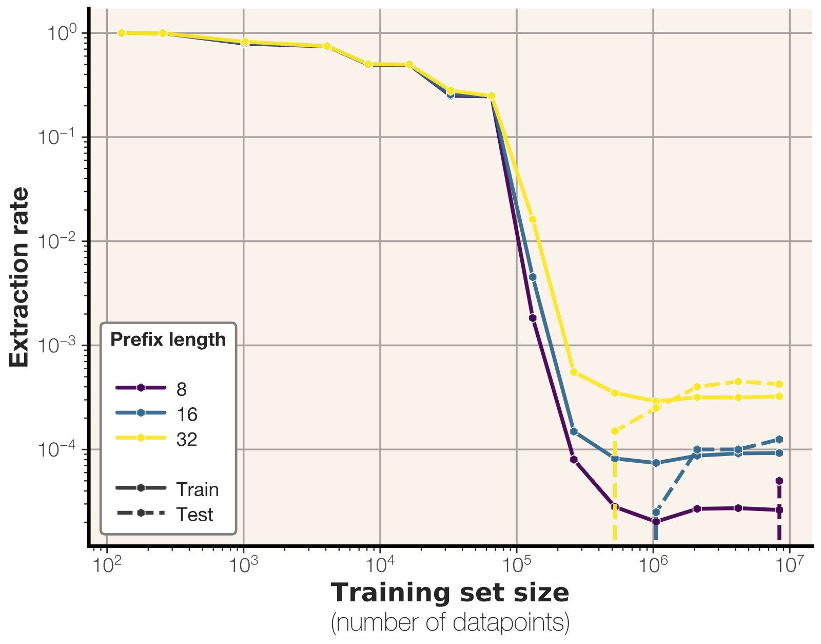
Figure 8: Extraction rates of 64-token training sequences across prefix lengths, for both train and evaluation.
图 8:64 个 token 的训练序列在不同前缀长度下的抽取率,分别给出训练集和评估集的结果。
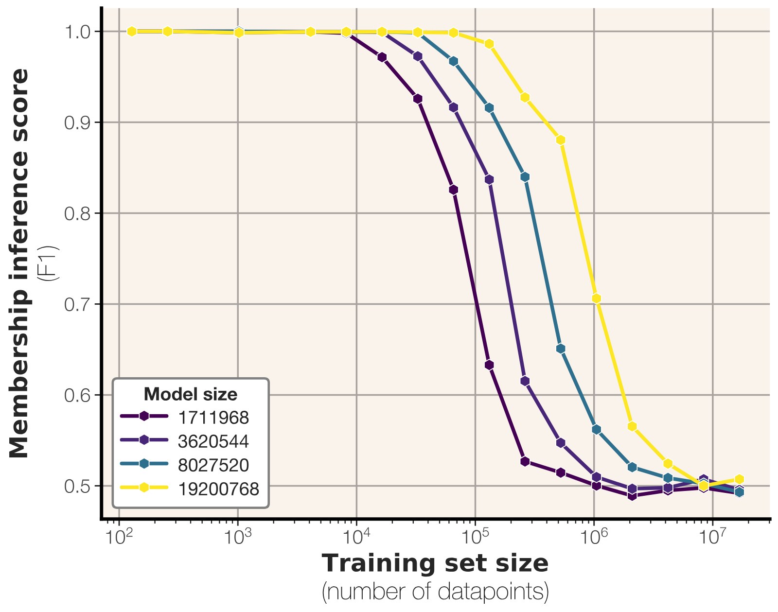
Figure 9: Membership inference F1 across dataset sizes. In this case, F1 score of 0.5 implies random guessing.
图 9:不同数据集规模下的成员推断 F1。在这种情形下,F1 为 0.5 意味着随机猜测。
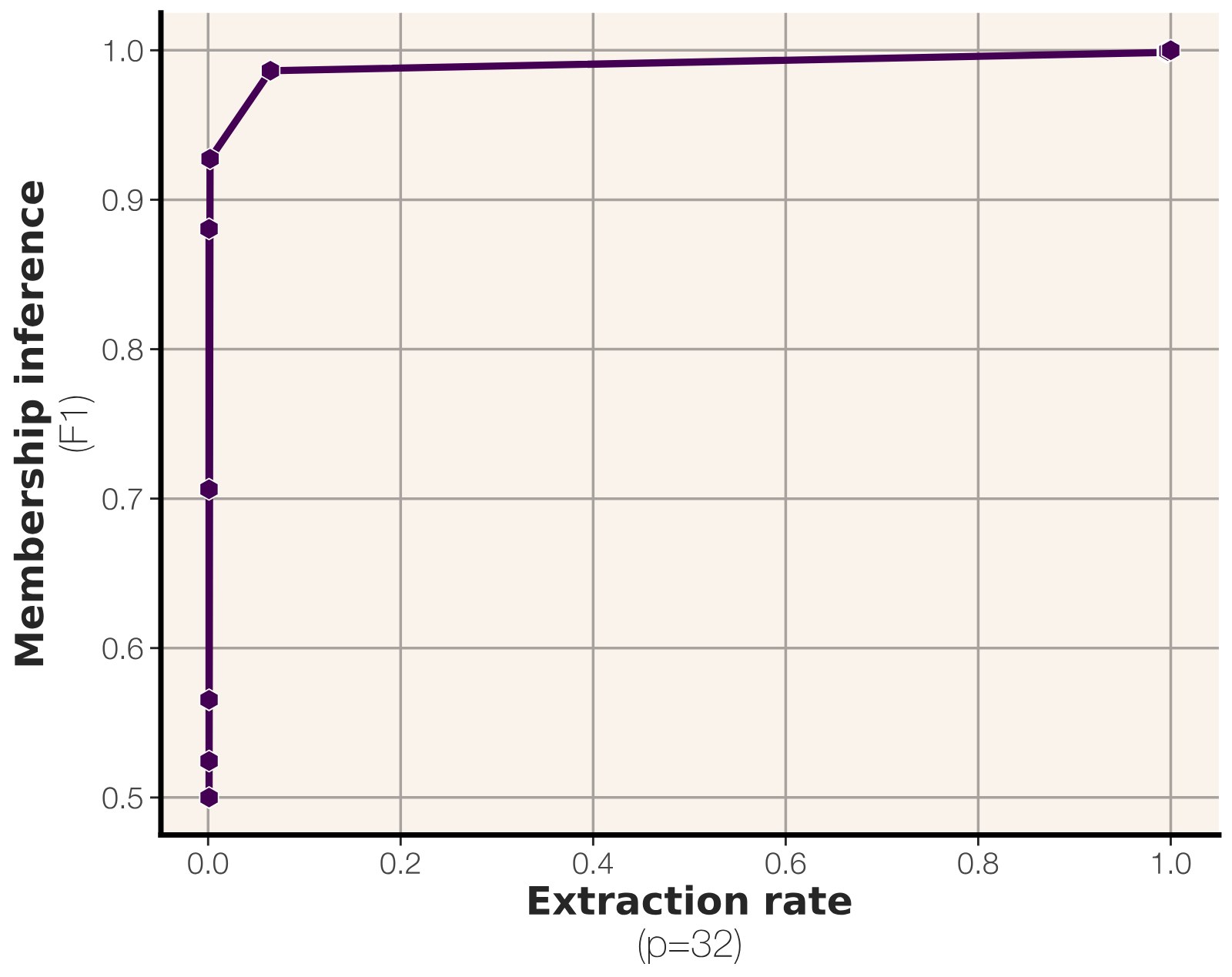
Figure 10: Membership inference vs 32-token-prefix suffix extraction rate. Membership inference is generally easier than extraction.
图 10:成员推断相对 32-token 前缀的后缀抽取率。成员推断通常比抽取更容易。
Generalization explains nonzero extraction rates.
泛化可以解释非零的抽取率。
We measure extraction rates on the full training set and 10,000 non-overlapping test samples (Figure 17). We note that for 32-token prefixes, 100% are extractable for very small training set sizes; predictably, all extraction numbers decrease with training set size. When the dataset sizes grows sufficiently large, the extraction rate does not go fully to zero; however, it converges to nearly exactly the test extraction rate. In other words, when our (deduplicated) dataset grows sufficiently large, all successful training data extraction is attributable to generalization.
我们在完整训练集和 10,000 条互不重叠的测试样本上测量抽取率(图 17)。我们注意到,对于 32-token 前缀,在训练集非常小时 100% 可被抽取;可以预料,所有抽取数字都随训练集变大而下降。当数据集变得足够大时,抽取率并不会完全降到零;不过,它会收敛到几乎恰好等于测试集抽取率。换句话说,当我们(已去重的)数据集变得足够大时,所有成功的训练数据抽取都可以归因于泛化。
5 Memorization and Membership
5 记忆与成员关系
Our training settings allow total control over the train and test data and come with perfect deduplication. This makes our setting ideal for studying the relationship between model size, dataset size, and membership inference success rate.
我们的训练设定可以对训练数据和测试数据做完全控制,并且具有彻底的去重。这使它很适合用来研究模型规模、数据集规模与成员推断成功率之间的关系。
All of our membership inference results come from a standard loss-based membership inference (Yeom et al., 2018; Sablayrolles et al., 2019). The method is very simple: we set a cutoff loss value to predict whether a sample is or is not a member of the training dataset.
我们所有的成员推断结果都来自标准的基于损失的成员推断(Yeom et al., 2018; Sablayrolles et al., 2019)。方法非常简单:设定一个损失截断值,以此来预测某条样本是否属于训练数据集。
5.1 Membership in synthetic and text data
5.1 合成数据与文本数据中的成员关系
Synthetic data.
合成数据。
For each of our models trained on synthetic data, we plot the success rate of the membership inference attack attack across dataset sizes. We show results in Figure 14. Above a certain dataset size, membership inference starts to fail in the average case. This finding indicates that if the dataset size is too large compared to the model, membership inference of an average training sample may not be possible.
对每个在合成数据上训练的模型,我们画出成员推断攻击成功率随数据集规模的变化,结果见图 14。超过某一数据集规模之后,成员推断在平均情形下开始失败。这一发现表明:若数据集相对模型过大,对一条平均训练样本做成员推断可能并不可行。
Text.
文本。
For each of our models trained on text, we use unused non-overlapping data from FineWeb to perform a standard loss-based membership inference (Yeom et al., 2018; Sablayrolles et al., 2019) on each model and plot performance across dataset sizes (10). For a fixed model size, membership inference gets more difficult as the size of the data increases. When comparing membership inference to extraction (Figure 10), membership inference is strictly higher in every case; in some cases we can infer training dataset membership quite well (score of ) with an extraction rate of .
对每个在文本上训练的模型,我们用 FineWeb 中未使用、且互不重叠的数据,对每个模型做标准的基于损失的成员推断(Yeom et al., 2018; Sablayrolles et al., 2019),并画出不同数据集规模下的性能(图 10)。在固定模型规模时,数据越大,成员推断越难。把成员推断与抽取比较(图 10),成员推断在所有情形下都严格更高;有时我们可以很好地推断训练集成员关系(分数为 ),而抽取率却是 。
5.2 Scaling laws for Membership
5.2 成员推断的缩放律
In this section we develop a set of predictive models for memorization. Specifically, we predict the F1 score of a loss-based membership attack given token count, number of examples, and model parameter count. We then validate our predictions on models from K to B parameters.
本节我们为记忆建立一组预测模型。具体来说,给定 token 数、样本数和模型参数量,我们预测基于损失的成员攻击的 F1 分数。然后在参数量从 K 到 B 的模型上验证这些预测。
5.2.1 Functional forms
5.2.1 函数形式
We observe that for a fixed model capacity, membership inference follows a roughly sigmoidal form with respect to dataset size. The intuitive explanation is that M.I. is easy for large models overfit to tiny datasets, so its score begin at 1; as dataset size increases, differentiating train from test data by loss becomes more and more difficult, eventually decaying toward 0.5.
我们观察到,在固定模型容量时,成员推断相对于数据集规模大致呈 sigmoid 形态。直观解释是:大型模型在很小的数据集上过拟合时,成员推断很容易,分数从 1 开始;随着数据集变大,用损失区分训练数据和测试数据变得越来越难,最终向 0.5 衰减。
We reuse the data collected in our text experiments (Section 4) to solve for constants in the following equation:
我们复用文本实验(第 4 节)中收集的数据,求解下列方程中的常数 :
where .
其中 。
Limiting behavior.
极限行为。
We observe that as , performance of our membership inference attack decreases to (essentially random performance). For a model trained on an infinite dataset, our law predicts both membership inference and extraction to be impossible.
我们观察到,当 时,成员推断攻击的性能下降到 (本质上是随机表现)。对在无限数据集上训练的模型,我们的定律预测成员推断和抽取都不可能。
Fitting.
拟合。
We use a non-linear least squares solver to find optimal values for . Solutions found are , , and . We plot the scaling laws along with observed data in Figure 7. Although the sigmoidal function is slightly simplistic (the points do not perfectly fit) our fit produces estimates within of observations.
我们用非线性最小二乘求解器寻找 的最优值。得到的解是 ,,以及 。我们在图 7 中画出缩放律以及观测数据。尽管 sigmoid 函数略显简化(各点并非完全落在曲线上),我们的拟合给出的估计与观测相差在 以内。
5.2.2 Validation on larger models
5.2.2 在更大模型上的验证
We note that all contemporary language models trained with a tokens-per-parameter ratio of or higher, which according to our laws would imply membership inference score of – that is, within our formulation, statistically significant loss-based membership inference is not possible.
我们注意到,当代语言模型都在每参数 个 token 或更高的配比下训练;按我们的定律,这将意味着成员推断分数为 ——也就是说,在我们的表述下,统计上显著的、基于损失的成员推断是不可能的。
| Predicted F1 | Observed F1 | |||||
|---|---|---|---|---|---|---|
| GPT2-XL | 1600 | 48 | 1,556,075,200 | 170,654,583 | 0.55 | |
| 76,795,021 | 0.75 | |||||
| 18,851,574 | 0.95 | |||||
| GPT2-Medium | 768 | 12 | 123,702,528 | 13,566,442 | 0.55 | |
| 6,104,935 | 0.75 | |||||
| 1,498,634 | 0.95 |
Table 2: Dataset sizes that our scaling law predicts will produce a given membership inference F1, along with empirical values.
| 预测 F1 | 观测 F1 | |||||
|---|---|---|---|---|---|---|
| GPT2-XL | 1600 | 48 | 1,556,075,200 | 170,654,583 | 0.55 | |
| 76,795,021 | 0.75 | |||||
| 18,851,574 | 0.95 | |||||
| GPT2-Medium | 768 | 12 | 123,702,528 | 13,566,442 | 0.55 | |
| 6,104,935 | 0.75 | |||||
| 1,498,634 | 0.95 |
表 2:缩放律预测会产生给定成员推断 F1 的数据集规模,以及相应的经验值。
To validate our predictions, we train models with expected membership scores of 0.55, 0.75, and 0.95. For model sizes we select GPT-2 small (M params) and GPT-2 XL (B params). Using our scaling law, we solve for the dataset size required to get the desired membership inference score for the given model size (see Table 2 for more information). We train models on the estimated dataset size and measure F1 score (shown as circles in Figure 7).
为验证预测,我们训练预期成员 分数为 0.55、0.75 和 0.95 的模型。模型规模上,我们选择 GPT-2 small(M 参数)和 GPT-2 XL(B 参数)。利用缩放律,我们求解在给定模型规模下要达到目标成员推断分数所需的数据集规模(更多信息见表 2)。我们在估计出的数据集规模上训练模型,并测量 F1 分数(在图 7 中以圆点表示)。
Our predictions are generally within points of the true F1 score; the score is most inaccurate for estimated F1 of 0.75, which is the point where the sigmoid is steepest. In general, the accuracy of our results indicates that our empirical model of membership inference is relatively accurate and provides evidence for why membership inference attacks fail on models trained on extremely large datasets (Das et al., 2024; Duan et al., 2024; Maini et al., 2024).
我们的预测通常与真实 F1 分数相差不超过 分;最不准的是估计 F1 为 0.75 的情形,也就是 sigmoid 最陡的位置。总体而言,这些结果的精度表明,我们关于成员推断的经验模型相对准确,并为何以成员推断攻击会在极大数据集上训练的模型上失败提供了证据(Das et al., 2024; Duan et al., 2024; Maini et al., 2024)。
6 Related Work
6 相关工作
Language models and compression.
语言模型与压缩。
Shannon’s source coding theorem (Shannon, 1948) first formalized the duality between prediction and compression. The connection between language modeling and compression was studied as far back as Shannon (1950), which observed that more accurate models of English can compress text in fewer bits. Other works note the connection between Kolmogorov complexity (Kolmogorov, 1965) and Shannon information in detail (Grunwald & Vitanyi, 2004). Delétang et al. (2024) investigate using modern transformer-based language models as compressors. We use compression as a tool to measure memorization in models.
Shannon 的信源编码定理(Shannon, 1948)首先形式化了预测与压缩之间的对偶。语言建模与压缩的联系早在 Shannon (1950) 就有研究,该文观察到更准确的英语模型可以用更少的比特压缩文本。其他工作详细指出了 Kolmogorov 复杂度(Kolmogorov, 1965)与 Shannon 信息之间的联系(Grunwald & Vitanyi, 2004)。Delétang et al. (2024) 研究把现代基于 Transformer 的语言模型当作压缩器来用。我们则把压缩当作测量模型记忆的工具。
Language model capacity.
语言模型的容量。
Early research on single-layer perceptrons found that single-layer networks can store up to 2 bits-per-parameter (Cover, 1965; Gardner, 1988; Baldi & Hornik, 1989). (Arpit et al., 2017) formalize the idea of effective capacity of a model and its training procedure; they also observe that both representation capacity and training time have a strong impact on empirical model capacity. Several other works measure language model capacity in the number of facts or random labels that can be memorized by a network such as an RNN (Collins et al., 2017; Boo et al., 2019) or transformer (Roberts et al., 2020; Heinzerling & Inui, 2021; Allen-Zhu & Li, 2024), sometimes under quantization. A few research efforts (Yun et al., 2019; Curth et al., 2023; Mahdavi et al., 2024; Kajitsuka & Sato, 2024) have developed theoretical estimates for the capacity of different model architectures, although none have yet scaled to multi-layer modern transformers. (Shwartz-Ziv et al., 2024) also analyze the ‘capacity’ of neural networks on datasets of varying size. We are the first to measure a clear upper-bound in model capacity using per-sample entropy measurements.
关于单层感知机的早期研究发现,单层网络最多可以存储每参数 2 比特(Cover, 1965; Gardner, 1988; Baldi & Hornik, 1989)。Arpit et al. (2017) 形式化了模型及其训练过程的有效容量概念;他们还观察到,表示容量和训练时间都对经验模型容量有很大影响。另有若干工作用网络能够记住的事实数或随机标签数来测量语言模型容量,对象包括 RNN(Collins et al., 2017; Boo et al., 2019)或 Transformer(Roberts et al., 2020; Heinzerling & Inui, 2021; Allen-Zhu & Li, 2024),有时还在量化设定下进行。也有一些研究(Yun et al., 2019; Curth et al., 2023; Mahdavi et al., 2024; Kajitsuka & Sato, 2024)为不同模型架构给出了容量的理论估计,但尚未扩展到多层的现代 Transformer。Shwartz-Ziv et al. (2024) 也分析了神经网络在不同规模数据集上的「容量」。我们是首个用逐样本熵测量给出模型容量清晰上界的工作。
Information regularization in learning theory.
学习理论中的信息正则。
Several works have explored the role of mutual information between the input and output of a learning algorithm (Bassily et al., 2018; Haghifam et al., 2020; Steinke & Zakynthinou, 2020). This concept closely relates to the notion of memorization based on Shannon information, discussed in Section 2.1. Some of our findings also relate to the discovery of double descent in machine learning (Belkin et al., 2019; Nakkiran et al., 2019) and language modeling (Xia et al., 2023), as well as general discussions of memorization and generalization in deep learning (Zhang et al., 2017; Tänzer et al., 2022).
若干工作探讨了学习算法输入与输出之间互信息的作用(Bassily et al., 2018; Haghifam et al., 2020; Steinke & Zakynthinou, 2020)。这一概念与第 2.1 节讨论的、基于 Shannon 信息的记忆概念密切相关。我们的一些发现也与机器学习(Belkin et al., 2019; Nakkiran et al., 2019)和语言建模(Xia et al., 2023)中的双重下降有关,以及深度学习中关于记忆与泛化的一般讨论(Zhang et al., 2017; Tänzer et al., 2022)。
Alternative definitions of memorization.
记忆的其他定义。
Unintended memorization is deeply related to the many other definitions of memorization proposed in the literature. We provide a detailed comparison in the following subsections.
非预期记忆与文献中提出的许多其他记忆定义有很深的关联。我们在下面几小节给出详细比较。
Prior definitions of memorization.
先前的记忆定义。
Carlini et al. (2019) defined a string as memorized by a language model if the second half of can be generated greedily when prompting the model with the first half. Following this, Nasr et al. (2023) introduced extractable memorization, where model is said to memorize if an adversarial prompt can be found that generates . Mireshghallah et al. (2022) and Schwarzschild et al. (2024) refined this definition by restricting to a certain number of tokens, preventing it from containing the entire . However, even this definition has limitations: for example, generating the sequence “cat cat cat … cat” with the prompt ”repeat cat 1000 times” does not necessarily indicate memorization. Carlini et al. (2019) use perplexity or likelihood, one measure of the compressibility of a sequence, in an effort to distinguish highly memorized sequences from merely easy-to-compress ones. One additional definition of note is counterfactual memorization (Zhang et al., 2023), which measures the impact of a single datapoint on training; this can be seen as an instantiation of our definition where a different model of the same family is used as a reference model. Overall, all these works regarded memorization in terms that can be seen as forms of compression, although did not explicitly define it as such.
Carlini et al. (2019) 把字符串 定义为被语言模型 记住,如果用 的前半部分提示模型时,后半部分可以被贪心生成。随后,Nasr et al. (2023) 引入了可抽取记忆:如果能找到一个对抗提示 使模型 生成 ,就称 记住了 。Mireshghallah et al. (2022) 和 Schwarzschild et al. (2024) 通过把 限制在一定 token 数之内、防止它包含整个 ,对这一定义做了细化。不过,即便这一定义也有局限:例如,用提示「repeat cat 1000 times」生成序列「cat cat cat … cat」,并不一定表明发生了记忆。Carlini et al. (2019) 使用困惑度或似然(这是序列可压缩性的一种度量),试图把高度被记住的序列与仅仅容易压缩的序列区分开。另一个值得注意的定义是反事实记忆(Zhang et al., 2023),它测量单个数据点对训练的影响;这可以看作我们定义的一种实例化,只不过参照模型换成了同一系列的另一个模型。总体而言,这些工作都把记忆理解为某种形式的压缩,尽管并未把它明确地这样定义。
Finally, a concurrent work (Cohen et al., 2024) proposes a theoretical definition for memorization also relying on Kolmogorov.
最后,一篇同期工作(Cohen et al., 2024)也提出了一种同样依赖 Kolmogorov 复杂度的记忆理论定义。
7 Conclusion
7 结论
We propose a new definition of memorization that allows us to measure the exact number of bits a model knows about a dataset. We use our definition to measure the capacity of modern transformer language models and analyze how measurements such as extraction and F1 score scale with model and dataset size. We also propose a scaling law for membership inference and validate it on larger models. Our results help further practitioner understanding of how language models memorize and what they might (or might not) be memorizing across model and dataset scales.
我们提出一种新的记忆定义,使我们能够测量模型对一个数据集精确知道多少比特。我们用这一定义测量现代 Transformer 语言模型的容量,并分析抽取和 F1 分数等指标如何随模型和数据集规模变化。我们还提出一条成员推断的缩放律,并在更大的模型上加以验证。这些结果有助于实践者进一步理解语言模型如何记忆,以及在不同模型和数据规模下它们可能记住了什么(或没有记住什么)。
8 Acknowledgements
8 致谢
Thanks to the many folks who helped us improve our paper, including Karen Ullrich, Niloofar Mireshghallah, Mark Ibrahim, Preetum Nakkiran, and Léon Bottou.
感谢许多帮助我们改进论文的人,包括 Karen Ullrich、Niloofar Mireshghallah、Mark Ibrahim、Preetum Nakkiran 和 Léon Bottou。
References
参考文献
Allen-Zhu & Li (2024) Allen-Zhu, Z. and Li, Y. Physics of language models: Part 3.3, knowledge capacity scaling laws, 2024. URL https://arxiv.org/abs/2404.05405 .
Arpit et al. (2017) Arpit, D., Jastrzebski, S., Ballas, N., Krueger, D., Bengio, E., Kanwal, M. S., Maharaj, T., Fischer, A., Courville, A., Bengio, Y., and Lacoste-Julien, S. A closer look at memorization in deep networks, 2017. URL https://arxiv.org/abs/1706.05394 .
Baldi & Hornik (1989) Baldi, P. and Hornik, K. Neural networks and principal component analysis: Learning from examples without local minima. Neural Networks , 2(1):53–58, 1989.
Bassily et al. (2018) Bassily, R., Moran, S., Nachum, I., Shafer, J., and Yehudayoff, A. Learners that use little information. In Algorithmic Learning Theory , pp. 25–55. PMLR, 2018.
Belkin et al. (2019) Belkin, M., Hsu, D., Ma, S., and Mandal, S. Reconciling modern machine-learning practice and the classical bias–variance trade-off. Proceedings of the National Academy of Sciences , 116(32):15849–15854, July 2019. ISSN 1091-6490. 10.1073/pnas.1903070116 . URL http://dx.doi.org/10.1073/pnas.1903070116 .
Bhattacharjee et al. (2023) Bhattacharjee, R., Dasgupta, S., and Chaudhuri, K. Data-copying in generative models: a formal framework. In International Conference on Machine Learning , pp. 2364–2396. PMLR, 2023.
Boo et al. (2019) Boo, Y., Shin, S., and Sung, W. Memorization capacity of deep neural networks under parameter quantization, 05 2019.
Brown et al. (2021) Brown, G., Bun, M., Feldman, V., Smith, A., and Talwar, K. When is memorization of irrelevant training data necessary for high-accuracy learning? In Proceedings of the 53rd annual ACM SIGACT symposium on theory of computing , pp. 123–132, 2021.
Carlini et al. (2019) Carlini, N., Liu, C., Úlfar Erlingsson, Kos, J., and Song, D. The secret sharer: Evaluating and testing unintended memorization in neural networks, 2019. URL https://arxiv.org/abs/1802.08232 .
Carlini et al. (2023a) Carlini, N., Hayes, J., Nasr, M., Jagielski, M., Sehwag, V., Tramèr, F., Balle, B., Ippolito, D., and Wallace, E. Extracting training data from diffusion models, 2023a. URL https://arxiv.org/abs/2301.13188 .
Carlini et al. (2023b) Carlini, N., Ippolito, D., Jagielski, M., Lee, K., Tramer, F., and Zhang, C. Quantifying memorization across neural language models, 2023b. URL https://arxiv.org/abs/2202.07646 .
Cohen et al. (2024) Cohen, E., Kaplan, H., Mansour, Y., Moran, S., Nissim, K., Stemmer, U., and Tsfadia, E. Data reconstruction: When you see it and when you don’t, 2024. URL https://arxiv.org/abs/2405.15753 .
Collins et al. (2017) Collins, J., Sohl-Dickstein, J., and Sussillo, D. Capacity and trainability in recurrent neural networks, 2017. URL https://arxiv.org/abs/1611.09913 .
Cover (1965) Cover, T. M. Geometrical and statistical properties of systems of linear inequalities with applications in pattern recognition. IEEE Transactions on Electronic Computers , EC-14(3):326–334, 1965.
Curth et al. (2023) Curth, A., Jeffares, A., and van der Schaar, M. A u-turn on double descent: Rethinking parameter counting in statistical learning, 2023. URL https://arxiv.org/abs/2310.18988 .
Das et al. (2024) Das, D., Zhang, J., and Tramèr, F. Blind baselines beat membership inference attacks for foundation models, 2024. URL https://arxiv.org/abs/2406.16201 .
Delétang et al. (2024) Delétang, G., Ruoss, A., Duquenne, P.-A., Catt, E., Genewein, T., Mattern, C., Grau-Moya, J., Wenliang, L. K., Aitchison, M., Orseau, L., Hutter, M., and Veness, J. Language modeling is compression, 2024. URL https://arxiv.org/abs/2309.10668 .
Duan et al. (2024) Duan, M., Suri, A., Mireshghallah, N., Min, S., Shi, W., Zettlemoyer, L., Tsvetkov, Y., Choi, Y., Evans, D., and Hajishirzi, H. Do membership inference attacks work on large language models? In Conference on Language Modeling (COLM) , 2024.
Dubey & et al (2024) Dubey, A. and et al, A. J. The llama 3 herd of models, 2024. URL https://arxiv.org/abs/2407.21783 .
Dwork (2006) Dwork, C. Differential privacy. In International Colloquium on Automata, Languages, and Programming , pp. 1–12. Springer, 2006.
Feldman (2020) Feldman, V. Does learning require memorization? a short tale about a long tail. In Proceedings of the 52nd Annual ACM SIGACT Symposium on Theory of Computing , pp. 954–959, 2020.
Gardner (1988) Gardner, E. The space of interactions in neural network models. Journal of Physics A: Mathematical and General , 21(1):257–270, 1988.
Geiping et al. (2024) Geiping, J., Stein, A., Shu, M., Saifullah, K., Wen, Y., and Goldstein, T. Coercing llms to do and reveal (almost) anything, 2024. URL https://arxiv.org/abs/2402.14020 .
Grunwald & Vitányi (2004) Grunwald, P. and Vitányi, P. Shannon information and kolmogorov complexity. arXiv preprint cs/0410002 , 2004.
Grunwald & Vitanyi (2004) Grunwald, P. and Vitanyi, P. Shannon information and kolmogorov complexity, 2004. URL https://arxiv.org/abs/cs/0410002 .
Haghifam et al. (2020) Haghifam, M., Negrea, J., Khisti, A., Roy, D. M., and Dziugaite, G. K. Sharpened generalization bounds based on conditional mutual information and an application to noisy, iterative algorithms. Advances in Neural Information Processing Systems , 33:9925–9935, 2020.
Heinzerling & Inui (2021) Heinzerling, B. and Inui, K. Language models as knowledge bases: On entity representations, storage capacity, and paraphrased queries, 2021. URL https://arxiv.org/abs/2008.09036 .
Jayaraman & Evans (2022) Jayaraman, B. and Evans, D. Are attribute inference attacks just imputation? In Proceedings of the 2022 ACM SIGSAC Conference on Computer and Communications Security , pp. 1569–1582, 2022.
Kajitsuka & Sato (2024) Kajitsuka, T. and Sato, I. Optimal memorization capacity of transformers, 2024. URL https://arxiv.org/abs/2409.17677 .
Kaplan et al. (2020) Kaplan, J., McCandlish, S., Henighan, T., Brown, T. B., Chess, B., Child, R., Gray, S., Radford, A., Wu, J., and Amodei, D. Scaling laws for neural language models, 2020. URL https://arxiv.org/abs/2001.08361 .
Kolmogorov (1963) Kolmogorov, A. N. On tables of random numbers. Sankhyā: The Indian Journal of Statistics, Series A , 25(4):369–376, 1963. URL http://www.jstor.org/stable/25049284 . Accessed: 21/12/2010 15:32.
Kolmogorov (1965) Kolmogorov, A. N. Three approaches to the quantitative definition of information. Problems of Information Transmission , 1(1):1–7, 1965.
Lee et al. (2022) Lee, K., Ippolito, D., Nystrom, A., Zhang, C., Eck, D., Callison-Burch, C., and Carlini, N. Deduplicating training data makes language models better, 2022. URL https://arxiv.org/abs/2107.06499 .
Lu et al. (2024) Lu, X., Li, X., Cheng, Q., Ding, K., Huang, X., and Qiu, X. Scaling laws for fact memorization of large language models, 2024. URL https://arxiv.org/abs/2406.15720 .
Mahdavi et al. (2024) Mahdavi, S., Liao, R., and Thrampoulidis, C. Memorization capacity of multi-head attention in transformers, 2024. URL https://arxiv.org/abs/2306.02010 .
Maini et al. (2024) Maini, P., Jia, H., Papernot, N., and Dziedzic, A. Llm dataset inference: Did you train on my dataset?, 2024. URL https://arxiv.org/abs/2406.06443 .
Mireshghallah et al. (2022) Mireshghallah, F., Uniyal, A., Wang, T., Evans, D., and Berg-Kirkpatrick, T. Memorization in nlp fine-tuning methods, 2022. URL https://arxiv.org/abs/2205.12506 .
Nakkiran et al. (2019) Nakkiran, P., Kaplun, G., Bansal, Y., Yang, T., Barak, B., and Sutskever, I. Deep double descent: Where bigger models and more data hurt, 2019. URL https://arxiv.org/abs/1912.02292 .
Nasr et al. (2023) Nasr, M., Carlini, N., Hayase, J., Jagielski, M., Cooper, A. F., Ippolito, D., Choquette-Choo, C. A., Wallace, E., Tramèr, F., and Lee, K. Scalable extraction of training data from (production) language models, 2023. URL https://arxiv.org/abs/2311.17035 .
Penedo et al. (2024) Penedo, G., Kydlíček, H., allal, L. B., Lozhkov, A., Mitchell, M., Raffel, C., Werra, L. V., and Wolf, T. The fineweb datasets: Decanting the web for the finest text data at scale, 2024. URL https://arxiv.org/abs/2406.17557 .
Prashanth et al. (2024) Prashanth, U. S., Deng, A., O’Brien, K., V, J. S., Khan, M. A., Borkar, J., Choquette-Choo, C. A., Fuehne, J. R., Biderman, S., Ke, T., Lee, K., and Saphra, N. Recite, reconstruct, recollect: Memorization in lms as a multifaceted phenomenon, 2024. URL https://arxiv.org/abs/2406.17746 .
Radford et al. (2019) Radford, A., Wu, J., Child, R., Luan, D., Amodei, D., and Sutskever, I. Language models are unsupervised multitask learners. 2019.
Roberts et al. (2020) Roberts, A., Raffel, C., and Shazeer, N. How much knowledge can you pack into the parameters of a language model?, 2020. URL https://arxiv.org/abs/2002.08910 .
Sablayrolles et al. (2019) Sablayrolles, A., Douze, M., Ollivier, Y., Schmid, C., and Jégou, H. White-box vs black-box: Bayes optimal strategies for membership inference, 2019. URL https://arxiv.org/abs/1908.11229 .
Schwarzschild et al. (2024) Schwarzschild, A., Feng, Z., Maini, P., Lipton, Z. C., and Kolter, J. Z. Rethinking llm memorization through the lens of adversarial compression, 2024. URL https://arxiv.org/abs/2404.15146 .
Shannon (1948) Shannon, C. E. A Mathematical Theory of Communication . University of Illinois Press, 1948. Reprint in 1998.
Shannon (1950) Shannon, C. E. Prediction and entropy of printed english, Sept 1950.
Shokri et al. (2017) Shokri, R., Stronati, M., Song, C., and Shmatikov, V. Membership inference attacks against machine learning models. In 2017 IEEE symposium on security and privacy (SP) , pp. 3–18. IEEE, 2017.
Shwartz-Ziv et al. (2024) Shwartz-Ziv, R., Goldblum, M., Bansal, A., Bruss, C. B., LeCun, Y., and Wilson, A. G. Just how flexible are neural networks in practice?, 2024. URL https://arxiv.org/abs/2406.11463 .
Steinke & Zakynthinou (2020) Steinke, T. and Zakynthinou, L. Reasoning about generalization via conditional mutual information. In Conference on Learning Theory , pp. 3437–3452. PMLR, 2020.
Tänzer et al. (2022) Tänzer, M., Ruder, S., and Rei, M. Memorisation versus generalisation in pre-trained language models, 2022. URL https://arxiv.org/abs/2105.00828 .
Xia et al. (2023) Xia, M., Artetxe, M., Zhou, C., Lin, X. V., Pasunuru, R., Chen, D., Zettlemoyer, L., and Stoyanov, V. Training trajectories of language models across scales, 2023. URL https://arxiv.org/abs/2212.09803 .
Xu et al. (2020) Xu, Y., Zhao, S., Song, J., Stewart, R., and Ermon, S. A theory of usable information under computational constraints, 2020. URL https://arxiv.org/abs/2002.10689 .
Yeom et al. (2018) Yeom, S., Giacomelli, I., Fredrikson, M., and Jha, S. Privacy risk in machine learning: Analyzing the connection to overfitting, 2018. URL https://arxiv.org/abs/1709.01604 .
Yun et al. (2019) Yun, C., Sra, S., and Jadbabaie, A. Small relu networks are powerful memorizers: a tight analysis of memorization capacity, 2019. URL https://arxiv.org/abs/1810.07770 .
Zhang et al. (2017) Zhang, C., Bengio, S., Hardt, M., Recht, B., and Vinyals, O. Understanding deep learning requires rethinking generalization, 2017. URL https://arxiv.org/abs/1611.03530 .
Zhang et al. (2023) Zhang, C., Ippolito, D., Lee, K., Jagielski, M., Tramèr, F., and Carlini, N. Counterfactual memorization in neural language models, 2023. URL https://arxiv.org/abs/2112.12938 .
Appendix A Appendix
附录 A 附录
A.1 How reliable are our linear estimates of capacity?
A.1 我们对容量的线性估计有多可靠?
| Params. | Memorized | Expected | Error | |
|---|---|---|---|---|
| 4 | 4.19 | |||
| 8 | 1.80 | |||
| 16 | 0.84 | |||
| 32 | 0.41 | |||
| 64 | 2.97 | |||
| 128 | 1.24 | |||
| 256 | 0.44 |
Table 3: Model capacity estimates across sequence length , along with error (%).
| 参数量 | 已记忆 | 预期 | 误差 | |
|---|---|---|---|---|
| 4 | 4.19 | |||
| 8 | 1.80 | |||
| 16 | 0.84 | |||
| 32 | 0.41 | |||
| 64 | 2.97 | |||
| 128 | 1.24 | |||
| 256 | 0.44 |
表 3:不同序列长度 下的模型容量估计,以及误差(%)。
| Params. | Memorized | Expected | Error | |
|---|---|---|---|---|
| 128 | 0.36 | |||
| 512 | 2.78 | |||
| 1024 | 2.70 | |||
| 2048 | 1.11 | |||
| 4096 | 0.47 |
Table 4: Model capacity estimates across vocab size , along with error (%).
| 参数量 | 已记忆 | 预期 | 误差 | |
|---|---|---|---|---|
| 128 | 0.36 | |||
| 512 | 2.78 | |||
| 1024 | 2.70 | |||
| 2048 | 1.11 | |||
| 4096 | 0.47 |
表 4:不同词表大小 下的模型容量估计,以及误差(%)。
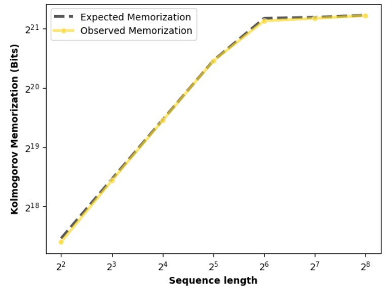
Figure 11: Model memorization across sequence lengths for a fixed-length dataset. Our predictions of total memorization are accurate, with an average error rate of 1.7%.
图 11:在固定总长度的数据集上,模型记忆量随序列长度的变化。我们对总记忆量的预测是准确的,平均误差率为 1.7%。
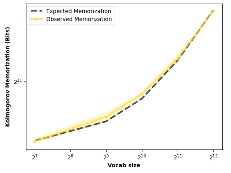
Figure 12: Model memorization across vocabulary size for a fixed-length dataset. Our predictions of total memorization are accurate, with an average error rate of 1.8%. Note that, we do not observe a capacity plateau, since increasing also increases parameters.
图 12:在固定总长度的数据集上,模型记忆量随词表大小的变化。我们对总记忆量的预测是准确的,平均误差率为 1.8%。需要注意,我们没有观察到容量平台,因为增大 同时也会增加参数量。
Instead of scaling the number of examples in a dataset, we scale model sequence length to adjust the size of a dataset. We use the following measurement for expected memorization of a model:
我们不再缩放数据集中的样本数,而是通过缩放模型序列长度来调整数据集大小。我们用下面的量来测量模型的预期记忆:
we substitute our previous estimate of and ensure to adjust the parameter count for increases due to resizing the model’s embedding matrices. We fix the number of training samples to and train a model with layers and a hidden size of . Results are illustrated in Figure 12 and Table 4. Our predictions of total memorization are accurate, with an average error rate of 1.7% while scaling and 1.8% when scaling .
我们代入先前估计的 ,并确保根据模型嵌入矩阵变大所增加的参数量调整参数计数。我们把训练样本数固定为 ,训练一个 层、隐藏维为 的模型。结果见图 12 和表 4。我们对总记忆量的预测是准确的:缩放 时平均误差率为 1.7%,缩放 时为 1.8%。
A.2 Additional memorization results
A.2 额外的记忆结果
Our findings indicate that memorization of text data neatly plateaus near the model capacity just as in the synthetic data case. When the dataset size increases by a factor of , the model divides its memorization between datapoints by an equal amount; the sum of memorization is measured to be constant, presumably at the upper bound of the model’s capacity.
我们的发现表明,文本数据的记忆会像合成数据那样,在接近模型容量处整齐地进入平台。当数据集规模增大 倍时,模型把记忆均匀地分到各条数据点上;测得的记忆总和保持不变,推测就在模型容量的上界。
When the dataset is small enough for each model to fit – that is, below the capacity of the smallest model – we observe very similar performance between the models. For larger data sizes we notice an interesting trend: unintended memorization increases with dataset size for to a point, presumably as a model fills its capacity with the available information, and then decreases, as the model replaces sample-level information with more useful, generalizable knowledge. A given model generalizes the most (and memorizes the least information about any individual sample) when the dataset is maximally large.
当数据集小到每个模型都能装下——也就是低于最小模型的容量——时,我们观察到各模型之间的表现非常接近。对更大的数据规模,我们注意到一个有意思的趋势:非预期记忆先随数据集增大而上升,到某一点为止,推测是模型用可获得的信息填满容量;随后下降,因为模型用更有用、可泛化的知识替换了样本级信息。当数据集最大时,给定模型泛化最多(并且对任何单个样本记住的信息最少)。
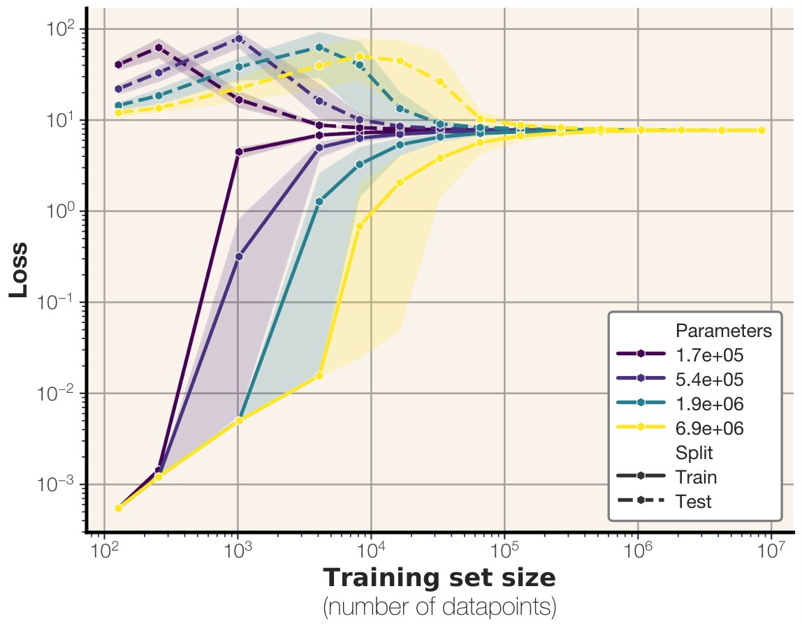
Figure 13: Train and test losses for different-sized language models trained on synthetic data.
图 13:在合成数据上训练的不同规模语言模型的训练损失和测试损失。
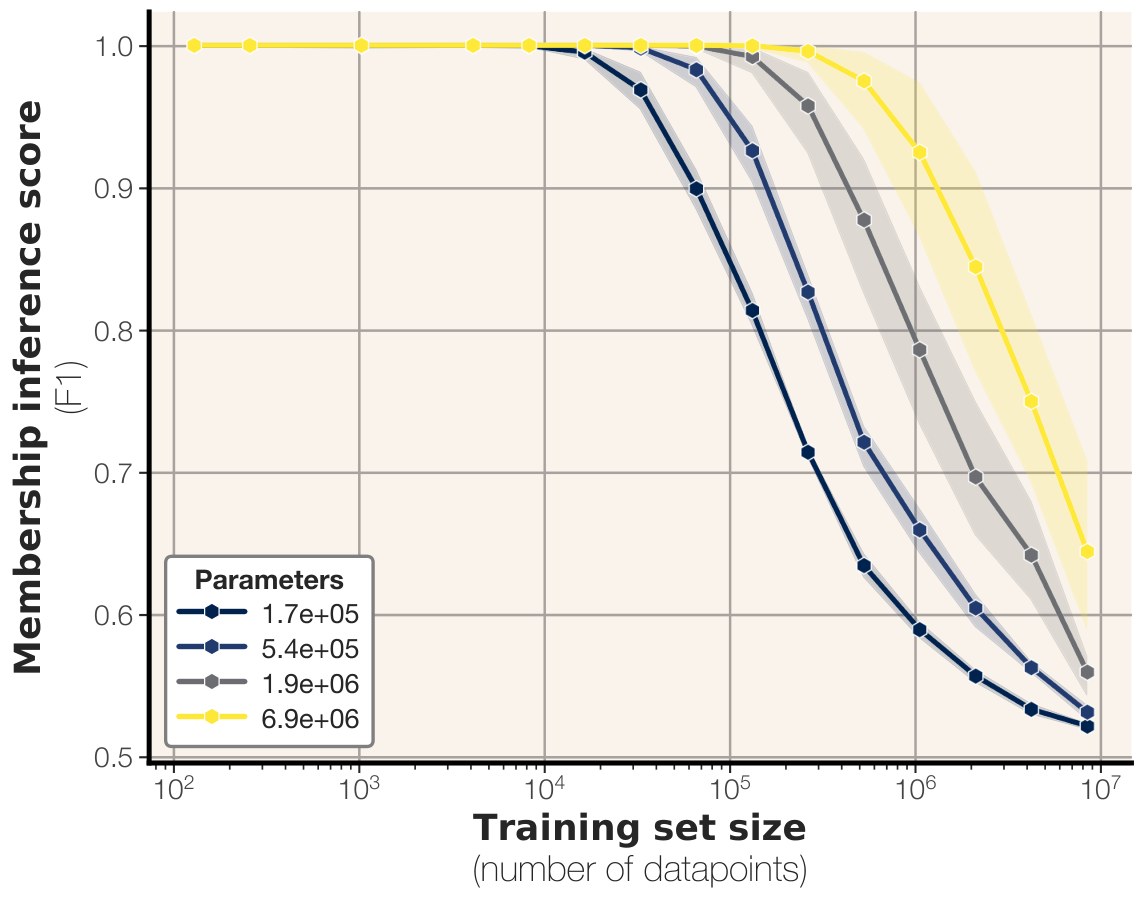
Figure 14: Membership inference attack performance decreases with dataset scale. In the case of uniform synthetic data, membership inference performance never falls below .
图 14:成员推断攻击的性能随数据集规模增大而下降。在均匀合成数据的情形下,成员推断性能从未落到 以下。
A.3 Comparison of distributions memorized
A.3 所记忆分布的比较
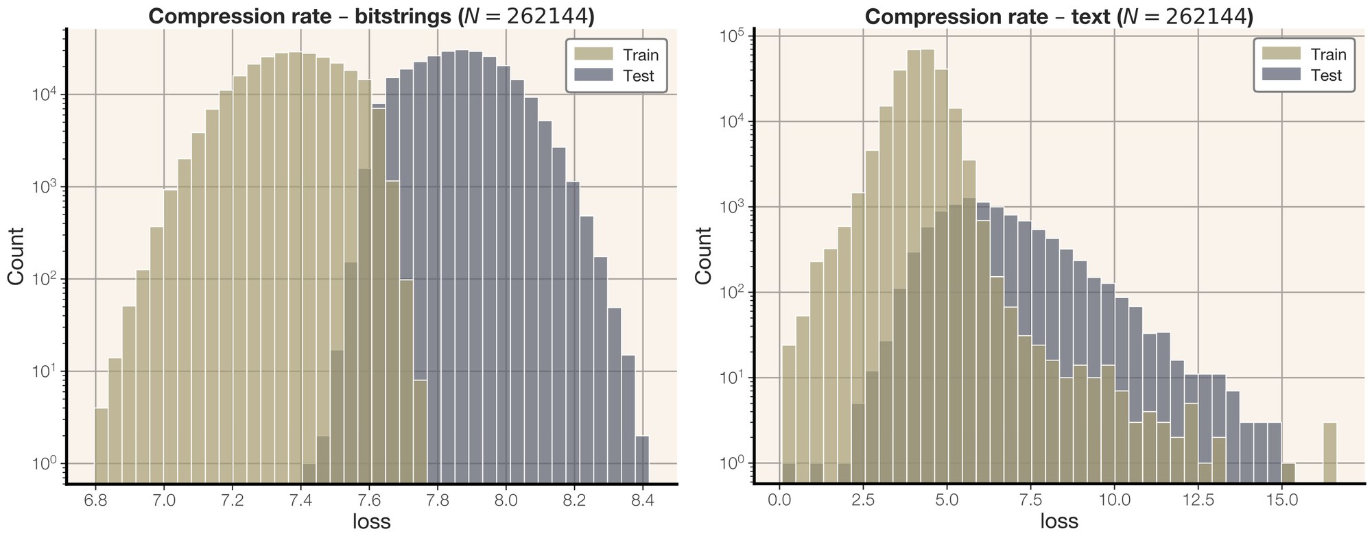
Figure 15: Distribution of compression rates for equal-sized transformers (, ) trained on sequences of equal-length random bitstrings (left) and text (right).
图 15:同等规模 Transformer(,)分别在 条等长随机比特串(左)和文本(右)上训练后,压缩率的分布。
Distribution-level analysis.
分布层面的分析。
Text sequences have very different properties than uniform synthetic bitstrings. We explore how two models of equal capacity spread their memorization across datapoints. We plot a histogram (Figure 15) of train and test compression rates of training data from both synthetic random bitstrings and text. Random training data follows a very normal distribution with a small amount of overlap between train and test compression rates. Text loss is lower on average but more spread out, with low loss on some training points and a long tail of higher losses. There is much more overlap between the train and test loss distributions, which explains why membership inference is more difficult for text data.
文本序列与均匀合成比特串有很不同的性质。我们考察两个容量相同的模型如何把记忆分配到各条数据点上。我们画出直方图(图 15),分别展示合成随机比特串和文本的训练数据在训练集与测试集上的压缩率。随机训练数据呈非常正态的分布,训练与测试压缩率只有少量重叠。文本的损失平均更低,但更分散:一些训练点损失很低,同时有一条更高损失的长尾。训练损失分布与测试损失分布的重叠要大得多,这解释了为什么文本数据上的成员推断更难。
Which datapoints are most memorized?
哪些数据点被记住得最多?
Our distribution-level analysis indicates that unlike in the random-bitstring case, models trained on a large amount of text are able to memorize a small number of datapoints. Prior work has indicated that a large amount of this memorization can be due to duplicated training points (Lee et al., 2022) but our dataset is fully deduplicated so this cannot be an explanation in our case.
分布层面的分析表明,与随机比特串的情形不同,在大量文本上训练的模型能够记住少量数据点。先前工作指出,这类记忆有很大一部分可能来自重复的训练点(Lee et al., 2022),但我们的数据集已完全去重,因此这不能作为我们情形下的解释。
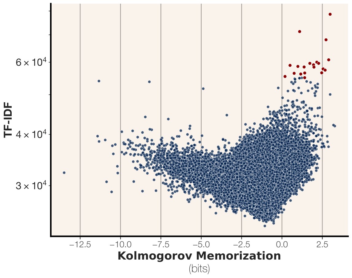
Figure 16: Unintended memorization vs. TF-IDF for all training points of a param model trained past its capacity on sequences of English text. The training documents with rarest words are typically the most memorized.
图 16:一个 参数的模型在超过其容量的 条英语文本序列上训练后,全部训练点的非预期记忆相对 TF-IDF。通常,含有最罕见词的训练文档被记住得最多。
To quantitatively evaluate the number of rare words per document, we measure the TF-IDF of each training document, plotted vs. unintended memorization in Figure 16. We use the following equation for TF-IDF:
为定量评估每篇文档中罕见词的数量,我们测量每个训练文档的 TF-IDF,并在图 16 中相对非预期记忆画出。我们使用下面的 TF-IDF 公式:
where indicates the total number of times word appears in dataset . Intuitively, a higher TF-IDF score for document indicates that contains more words that are rare in .
其中 表示词 在数据集 中出现的总次数。直观上,文档 的 TF-IDF 分数更高,意味着 包含更多在 中罕见的词。
We clearly observe for samples with positive unintended memorization there is a strong correlation between trainset TF-IDF and memorization: examples with more rare words are more memorized. In particular, the sample with highest TF-IDF out of the whole training dataset (a sequence of Japanese words) has the third-highest measured memorization; even though this is just one out of training samples, the model can regurgitate the entire sequence given just a single token (
我们清楚地观察到,对非预期记忆为正的样本,训练集 TF-IDF 与记忆之间有很强的相关:含有更多罕见词的例子被记住得更多。特别是,整个训练集中 TF-IDF 最高的样本(一段日语词)测得的记忆量排在第三;即便它只是 条训练样本中的一条,模型在只给定一个 token(
囚). Out of the top twenty memorized sequences, all but three contain sequences of tokens from other languages (Japanese, Chinese, and Hebrew).
囚)时就能复述整个序列。在被记住最多的前二十条序列中,除了三条以外,都包含来自其他语言(日语、中文和希伯来语)的 token 序列。
Manual analysis (Table 5) indicates that the most memorized datapoints have extremely rare tokens, typically ones not found in English.
人工分析(表 5)表明,被记住最多的数据点具有极为罕见的 token,通常是英语中找不到的那些。
Table 5: Highest TF-IDF training examples from a param model trained past its capacity on sequences of English text. All of the highest TF-IDF examples are considered memorized, and contain text from non-English languages (Japanese, Chinese, Hebrew, and Greek).
表 5:一个 参数的模型在超过其容量的 条英语文本序列上训练后,TF-IDF 最高的训练例子。所有最高 TF-IDF 的例子都被视为已记住,并且包含非英语文本(日语、中文、希伯来语和希腊语)。
A.4 Scaling law fit
A.4 缩放律的拟合
Here we demonstrate the fit of our sigmoidal scaling law to experimental data. We show points in tokens-per-parameter vs. fit in Figure 17. Although the sigmoidal function is slightly simplistic (the points do not perfectly fit the curve) our fit produces estimates within of observations.
这里我们展示 sigmoid 缩放律对实验数据的拟合。我们在图 17 中画出以每参数 token 数计的各点与拟合曲线。尽管 sigmoid 函数略显简化(各点并非完全落在曲线上),我们的拟合给出的估计与观测相差在 以内。
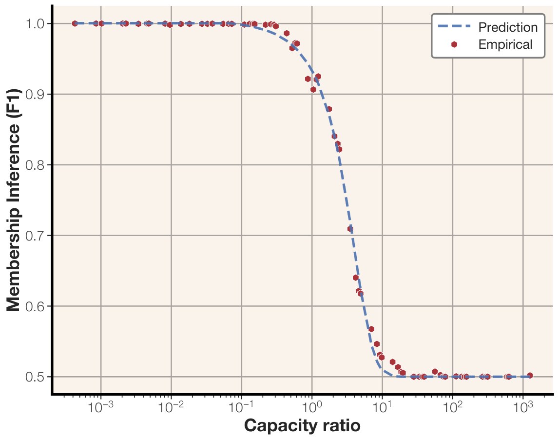
Figure 17: Our sigmoidal scaling law for membership inference fit to experimental data.
图 17:我们为成员推断提出的 sigmoid 缩放律对实验数据的拟合。
A.5 Proofs
A.5 证明
In the section we provide the proofs missing from the main body.
本节给出正文中省略的证明。
A.6 Proof of Proposition 1
A.6 命题 1 的证明
Here we prove Proposition 1
这里我们证明命题 1。
Proof.
证明。
we have
我们有
And since the data is sampled i.i.d., all random variables in are independent. [^4] So we have,
又由于数据是独立同分布采样的,集合 中的所有随机变量都是独立的。[^4] 因此我们有
which implies
从而得到
On the other hand, we have
另一方面,我们有
∎
A.7 Proof of Proposition 4
A.7 命题 4 的证明
Proof.
证明。
We first state a Lemma about connection between algorithmic (kolmogorov) mutual information and mutual information.
我们先陈述一条关于算法(Kolmogorov)互信息与互信息之间联系的引理。
Lemma 6.
引理 6。
[Theorem 3.6 in Grunwald & Vitányi (2004)] Assume be a pair of joint random variables. Let be the density function, Then we have
[Grunwald & Vitányi (2004) 中的定理 3.6]设 是一对联合随机变量。设 为密度函数,。则有
Now we use this lemma to prove the statement of the Proposition. Let be a the density function for the joint distribution . That is . Note that this function is independent of . By definition we have
现在用这条引理来证明命题的陈述。设 是联合分布 的密度函数,即 。注意这个函数与 无关。按定义我们有
Now using Lemma 6 we have
现在利用引理 6,我们有
and this concludes the statement of Proposition by setting ∎
令 ,即得命题的结论。∎
A.8 Limitations
A.8 局限
Our efforts to measure language model memorization come from a line of recent research to discover whether models have analyzed certain texts, and if so, how much. However, our main experimental contributions relate to the practice of training and evaluating language models, including a new perspective on the phenomenon of grokking (Nakkiran et al., 2019) and a new measurement of capacity. Our results are specific to the environment proposed and do not necessarily generalize to other datasets, architectures, or training setups.
我们测量语言模型记忆的努力,来自近期一系列研究:它们想发现模型是否分析过某些文本,以及如果分析过,程度有多大。不过,我们主要的实验贡献与训练和评估语言模型的实践有关,包括对 grokking 现象(Nakkiran et al., 2019)的新视角,以及对容量的新测量。我们的结果针对所提出的环境,并不必然推广到其他数据集、架构或训练设定。
Appendix B Discussion of other notions of memorization
附录 B 对其他记忆概念的讨论
In this section we list multiple other notions of memorization and compare it with our definition. We specifically focus on why these notions do not satisfy all of our requirements.
本节列出多种其他记忆概念,并与我们的定义加以比较。我们特别关注这些概念为何不能满足我们的全部要求。
- Stability-based notions of memorization. There are notions of privacy and memorization that deal with “stability” of the training algorithm to small changes in the training set. Most notably, differential privacy Dwork (2006) considers the worst-cast drift of the model distribution when a single data point changes. Another notion of memorization in Feldman (2020) is based on the change of the model prediction on a point , when we add the labeled pair to the training set of a classification/regression model. Both of these notions are crucially relying on the learning algorithm and how it behaves. Moreover, the definition of differential privacy is not ideal for our case because it is a worst-case definition and cannot be applied at sample/model level. While the notion of memorization in Feldman (2020) does not have this particular issue, it suffers from the fact that it only applies to classification models and mostly deals with the memorization of the association between the label () and input (), and not the memorization of itself. These issues make these notions not ideal for our case.
- 基于稳定性的记忆概念。 有一些隐私和记忆概念处理训练算法对训练集微小变化的「稳定性」。最著名的是差分隐私(Dwork, 2006),它考虑单个数据点变化时模型分布的最坏情况漂移。Feldman (2020) 中的另一种记忆概念,则基于把带标签的对 加入分类/回归模型的训练集后,模型在点 上预测的变化。这两种概念都关键地依赖于学习算法及其行为。此外,差分隐私的定义对我们并不理想,因为它是最坏情况定义,不能在样本/模型层面应用。Feldman (2020) 的记忆概念虽然没有这个问题,却有另一不足:它只适用于分类模型,并且主要处理的是标签()与输入()之间关联的记忆,而不是对 本身的记忆。这些使得它们对我们的情形并不理想。
- Extraction-based memorization. There are multiple works in the literature (Carlini et al., 2019; Mireshghallah et al., 2022; Nasr et al., 2023; Zhang et al., 2023; Carlini et al., 2023b; Schwarzschild et al., 2024) that define memorization of samples in language models based on how easy it is to extract that sample. Specifically, when trying to understand the extent of memorization of a sample in a model they measure some notion of complexity for the task of eliciting the model to output . Although these notions are great in that they only take a model and a sample , they still do not account for generalization. Considering our running example of the following training sample: ”What is ? (A: )”, this will be identified as highly memorized by almost all of the extraction based notions of memorization. Another issue with these definitions are that they are heavily dependent on the details of decoding algorithm. This is not ideal as we do not expect the memorization of a sample in a model to depend on the detailed parameters we use to generate samples using . The work of Schwarzschild et al. (2024) in this category is the closest to ours. This work which is based on prompt-optimization, optimizes a short prompt to make the model elicit , then it calls the sample memorized, if length of is less than . Although this definition is close to our definition in using compression, it still does not account for generalization of the model. Moreover, it focuses on a specific way of compression through prompting. We posit that compression through prompting is an inferior compression scheme and can often lead to compression rates greater than 1.
- 基于抽取的记忆。 文献中有多项工作(Carlini et al., 2019; Mireshghallah et al., 2022; Nasr et al., 2023; Zhang et al., 2023; Carlini et al., 2023b; Schwarzschild et al., 2024)根据把样本从语言模型中抽取出来有多容易,来定义样本的记忆。具体来说,当试图理解样本 在模型 中被记住的程度时,它们测量诱使模型输出 这一任务的某种复杂度。这些概念的优点是只依赖模型 和样本 ,但仍然没有把泛化考虑进去。回到我们一直使用的训练样本例子:「What is ?(A: )」,几乎所有基于抽取的记忆概念都会把它判定为高度被记住。这些定义的另一个问题是,它们严重依赖于解码算法的细节。这并不理想,因为我们并不期望样本 在模型 中的记忆,会依赖于我们用 生成样本时所采用的具体参数。这一类中与我们最接近的是 Schwarzschild et al. (2024)。这项基于提示优化的工作优化一个短提示 ,使模型引出 ,如果 的长度小于 ,就把样本 称为被记住。虽然这一定义在使用压缩这一点上接近我们的定义,它仍然没有考虑模型的泛化。此外,它只关注通过提示这一种压缩方式。我们认为,通过提示做压缩是较差的压缩方案,常常会得到大于 1 的压缩率。
- Membership/attribute inference. Membership inference Shokri et al. (2017) and attribute inference attacks Jayaraman & Evans (2022) have been used for empirically measuring the privacy of machine learning algorithms. These notions which usually aim at approximating the stability notions of memorization are suffering from the same shortcomings. They rely heavily on the learning algorithm and the data distribution. Moreover, they fail at providing a sample level notion of memorization. For example, the obtained accuracy for membership inference attack is only meaningful in the population level. This is because various attack may have different true positives for membership, and the union of all these true positive across different attack may cover the entire training set, rendering it unusable as a sample level notion of memorization.
- 成员/属性推断。 成员推断(Shokri et al., 2017)和属性推断攻击(Jayaraman & Evans, 2022)一直被用来经验地测量机器学习算法的隐私。这些概念通常旨在近似基于稳定性的记忆概念,因而也有同样的不足。它们严重依赖学习算法和数据分布。此外,它们无法提供样本级的记忆概念。例如,成员推断攻击得到的准确率只在总体层面有意义。这是因为不同攻击可能有不同的成员真正例,而这些真正例在不同攻击上的并集可能覆盖整个训练集,从而无法作为样本级的记忆概念来使用。
- Data copying in generative models. There are some interesting notions of memorization designed specifically for generative modeling where a generative model may output a certain portion of training samples (Bhattacharjee et al., 2023; Carlini et al., 2023a). These notions are similar to extraction based definition of memorization but they are more lenient in that they only require extraction of part of the training data. However, they still suffer from the same challenges as of extraction based definitions.
- 生成模型中的数据复制。 还有一些有意思的记忆概念是专门为生成建模设计的,其中生成模型可能输出训练样本的某一部分(Bhattacharjee et al., 2023; Carlini et al., 2023a)。这些概念类似于基于抽取的记忆定义,但更宽松,因为它们只要求抽取训练数据的一部分。不过,它们仍然具有基于抽取的定义所面临的同样困难。