HiFi-GAN: Generative Adversarial Networks for Efficient and High Fidelity Speech Synthesis
HiFi-GAN: Generative Adversarial Networks for Efficient and High Fidelity Speech Synthesis
HiFi-GAN:面向高效高保真语音合成的生成对抗网络
Jungil Kong Affiliation: Kakao Enterprise Email: henry.k@kakaoenterprise.com Jaehyeon Kim Affiliation: Kakao Enterprise Email: jay.xyz@kakaoenterprise.com Jaekyoung Bae Affiliation: Kakao Enterprise Email: storm.b@kakaoenterprise.com
Abstract
摘要
Several recent work on speech synthesis have employed generative adversarial networks (GANs) to produce raw waveforms. Although such methods improve the sampling efficiency and memory usage, their sample quality has not yet reached that of autoregressive and flow-based generative models. In this work, we propose HiFi-GAN, which achieves both efficient and high-fidelity speech synthesis. As speech audio consists of sinusoidal signals with various periods, we demonstrate that modeling periodic patterns of an audio is crucial for enhancing sample quality. A subjective human evaluation (mean opinion score, MOS) of a single speaker dataset indicates that our proposed method demonstrates similarity to human quality while generating 22.05 kHz high-fidelity audio 167.9 times faster than real-time on a single V100 GPU. We further show the generality of HiFi-GAN to the mel-spectrogram inversion of unseen speakers and end-to-end speech synthesis. Finally, a small footprint version of HiFi-GAN generates samples 13.4 times faster than real-time on CPU with comparable quality to an autoregressive counterpart.
近期若干语音合成工作用生成对抗网络(GAN)直接生成原始波形。这类方法提升了采样效率与显存利用率,但样本质量尚未赶上自回归与基于流的生成模型。本文提出 HiFi-GAN,在效率与高保真两方面同时达标。语音由多种周期的正弦成分构成,我们表明对周期模式建模对提升样本质量至关重要。在单说话人数据集上的主观评测(平均意见分,MOS)显示,该方法在单块 V100 GPU 上生成 22.05 kHz 高保真音频时,相对实时快 167.9 倍,听感接近真人。我们还展示了 HiFi-GAN 对未见说话人的梅尔频谱反演以及端到端语音合成的通用性。最后,一个小体积版本在 CPU 上相对实时快 13.4 倍,质量可与自回归对照模型相比。
1 Introduction
1 引言
Voice is one of the most frequent and naturally used communication interfaces for humans. With recent developments in technology, voice is being used as a main interface in artificial intelligence (AI) voice assistant services such as Amazon Alexa, and it is also widely used in automobiles, smart homes and so forth. Accordingly, with the increase in demand for people to converse with machines, technology that synthesizes natural speech like human speech is being actively studied.
语音是人类最常用、最自然的沟通接口之一。随着技术发展,语音正成为 Amazon Alexa 等人工智能语音助手的主界面,也广泛出现在汽车、智能家居等场景。人们与机器对话的需求上升,合成听起来像真人的自然语音也因此成为活跃研究方向。
Recently, with the development of neural networks, speech synthesis technology has made a rapid progress. Most neural speech synthesis models use a two-stage pipeline: 1) predicting a low resolution intermediate representation such as mel-spectrograms (Shen et al. 2018, Ping et al. 2017, Li et al. 2019) or linguistic features (Oord et al. 2016) from text, and 2) synthesizing raw waveform audio from the intermediate representation (Oord et al. 2016, Oord et al. 2018, Prenger et al. 2019, Kumar et al. 2019). The first stage is to model low-level representations of human speech from text, whereas the second stage model synthesizes raw waveforms with up to 24,000 samples per second and up to 16 bit fidelity. In this work, we focus on designing a second stage model that efficiently synthesizes high fidelity waveforms from mel-spectrograms.
近年神经网络推动语音合成快速进步。多数神经语音合成采用两阶段流水线:1)从文本预测低分辨率中间表示,如梅尔频谱(Shen 等 2018、Ping 等 2017、Li 等 2019)或语言学特征(Oord 等 2016);2)再由中间表示合成原始波形(Oord 等 2016、Oord 等 2018、Prenger 等 2019、Kumar 等 2019)。第一阶段从文本建模语音的低层表示,第二阶段则合成每秒最多约 24,000 个采样点、最高约 16 bit 保真度的原始波形。本文聚焦设计第二阶段模型:从梅尔频谱高效合成高保真波形。
Various work have been conducted to improve the audio synthesis quality and efficiency of second stage models. WaveNet (Oord et al. 2016) is an autoregressive (AR) convolutional neural network that demonstrates the ability of neural network based methods to surpass conventional methods in quality. However, because of the AR structure, WaveNet generates one sample at each forward operation; it is prohibitively slow in synthesizing high temporal resolution audio. Flow-based generative models are proposed to address this problem. Because of their ability to model raw waveforms by transforming noise sequences of the same size in parallel, flow-based generative models fully utilize modern parallel computing processors to speed up sampling. Parallel WaveNet (Oord et al. 2018) is an inverse autoregressive flow (IAF) that is trained to minimize its Kullback-Leibler divergence from a pre-trained WaveNet called a teacher. Compared to the teacher model, it improves the synthesis speed to 1,000 times or more, without quality degradation. WaveGlow (Prenger et al. 2019) eliminates the need for distilling a teacher model, and simplifies the learning process through maximum likelihood estimation by employing efficient bijective flows based on Glow (Kingma and Dhariwal 2018). It also produces high-quality audio compared to WaveNet. However, it requires many parameters for its deep architecture with over 90 layers.
已有大量工作提升第二阶段的音质与效率。WaveNet(Oord 等 2016)是自回归(AR)卷积网络,证明基于神经网络的方法可在质量上超越传统手段。但因 AR 结构,每次前向只出一点,合成高时间分辨率音频极慢。基于流的生成模型试图解决这一问题:它们能并行把同尺寸噪声序列变成原始波形,从而充分利用现代并行处理器加速采样。Parallel WaveNet(Oord 等 2018)是逆自回归流(IAF),训练时最小化相对预训练 WaveNet(教师)的 Kullback-Leibler 散度;相对教师,合成速度提升一千倍以上且不掉质量。WaveGlow(Prenger 等 2019)不再需要蒸馏教师,借助基于 Glow(Kingma 与 Dhariwal 2018)的高效双射流,用最大似然简化学习,音质也可与 WaveNet 相比;但其深度超过 90 层,参数量很大。
Generative adversarial networks (GANs) (Goodfellow et al. 2014), which are one of the most dominant deep generative models, have also been applied to speech synthesis. Kumar et al. 2019 proposed a multi-scale architecture for discriminators operating on multiple scales of raw waveforms. With sophisticated architectural consideration, the MelGAN generator is compact enough to enable real-time synthesis on CPU. Yamamoto et al. 2020 proposed multi-resolution STFT loss function to improve and stabilize GAN training and achieved better parameter efficiency and less training time than an IAF model, ClariNet (Ping et al. 2018). Instead of mel-spectrograms, GAN-TTS (Bińkowski et al. 2019) successfully generates high quality raw audio waveforms from linguistic features through multiple discriminators operating on different window sizes. The model also shows fewer FLOPs compared to Parallel WaveNet. Despite the advantages, there is still a gap in sample quality between the GAN models and AR or flow-based models.
生成对抗网络(GAN)(Goodfellow 等 2014)作为主流深度生成模型之一,也被用于语音合成。Kumar 等 2019 提出在原始波形多个尺度上工作的多尺度判别器结构;经细致结构设计,MelGAN 生成器足够紧凑,可在 CPU 上实时合成。Yamamoto 等 2020 提出多分辨率 STFT 损失以改进并稳定 GAN 训练,相对 IAF 模型 ClariNet(Ping 等 2018)参数更省、训练更短。GAN-TTS(Bińkowski 等 2019)不走梅尔频谱,而从语言学特征出发,用多个不同窗长的判别器成功生成高质量原始音频,FLOPs 也少于 Parallel WaveNet。尽管有这些优势,GAN 模型与 AR 或流模型之间仍有样本质量差距。
We propose HiFi-GAN, which achieves both higher computational efficiency and sample quality than AR or flow-based models. As speech audio consists of sinusoidal signals with various periods, modeling the periodic patterns matters to generate realistic speech audio. Therefore, we propose a discriminator which consists of small sub-discriminators, each of which obtains only a specific periodic parts of raw waveforms. This architecture is the very ground of our model successfully synthesizing realistic speech audio. As we extract different parts of audio for the discriminator, we also design a module that places multiple residual blocks each of which observes patterns of various lengths in parallel, and apply it to the generator.
我们提出 HiFi-GAN,在计算效率与样本质量上同时优于 AR 与流模型。语音由多种周期的正弦信号组成,对周期模式建模对生成逼真语音至关重要。因此我们提出由多个小子判别器构成的判别器,每个子判别器只看到原始波形中特定周期位置的部分。正是这一结构,使模型能成功合成逼真语音。既然判别器看的是不同片段,我们也在生成器里设计模块:并列放置多个残差块,各自观察不同长度的模式。
HiFi-GAN achieves a higher MOS score than the best publicly available models, WaveNet and WaveGlow. It synthesizes human-quality speech audio at speed of 3.7 MHz on a single V100 GPU. We further show the generality of HiFi-GAN to the mel-spectrogram inversion of unseen speakers and end-to-end speech synthesis. Finally, the tiny footprint version of HiFi-GAN requires only 0.92M parameters while outperforming the best publicly available models and the fastest version of HiFi-GAN samples 13.44 times faster than real-time on CPU and 1,186 times faster than real-time on single V100 GPU with comparable quality to an autoregressive counterpart.
HiFi-GAN 的 MOS 高于当时公开最好的 WaveNet 与 WaveGlow,可在单块 V100 GPU 上以 3.7 MHz 速度合成接近真人的语音。我们还展示了其对未见说话人梅尔频谱反演与端到端语音合成的通用性。小体积版本仅约 0.92M 参数,仍优于当时公开最佳模型;最快版本在 CPU 上相对实时快 13.44 倍、单块 V100 上快 1,186 倍,质量可与自回归对照相比。
Our audio samples are available on the demo web-site[^1], and we provide the implementation as open source for reproducibility and future work.[^2]
试听样例见演示网站[^1],实现已开源以便复现与后续研究。[^2]
2 HiFi-GAN
2.1 Overview
2.1 概述
HiFi-GAN consists of one generator and two discriminators: multi-scale and multi-period discriminators. The generator and discriminators are trained adversarially, along with two additional losses for improving training stability and model performance.
HiFi-GAN 由一个生成器与两个判别器组成:多尺度判别器与多周期判别器。生成器与判别器对抗训练,另加两项损失以提升训练稳定性与模型表现。
2.2 Generator
2.2 生成器
The generator is a fully convolutional neural network. It uses a mel-spectrogram as input and upsamples it through transposed convolutions until the length of the output sequence matches the temporal resolution of raw waveforms. Every transposed convolution is followed by a multi-receptive field fusion (MRF) module, which we describe in the next paragraph. Figure 1 shows the architecture of the generator. As in previous work (Mathieu et al. 2015, Isola et al. 2017, Kumar et al. 2019), noise is not given to the generator as an additional input.
生成器是全卷积网络。输入为梅尔频谱,经转置卷积逐步上采样,直到输出序列长度与原始波形时间分辨率一致。每次转置卷积后接多感受野融合(MRF)模块,下一小节说明。图 1 给出生成器结构。与先前工作(Mathieu 等 2015、Isola 等 2017、Kumar 等 2019)一样,不向生成器额外输入噪声。
Multi-Receptive Field Fusion
We design the multi-receptive field fusion (MRF) module for our generator, which observes patterns of various lengths in parallel. Specifically, MRF module returns the sum of outputs from multiple residual blocks. Different kernel sizes and dilation rates are selected for each residual block to form diverse receptive field patterns. The architectures of MRF module and a residual block are shown in Figure 1. We left some adjustable parameters in the generator; the hidden dimension , kernel sizes of the transposed convolutions, kernel sizes , and dilation rates of MRF modules can be regulated to match one’s own requirement in a trade-off between synthesis efficiency and sample quality.
多感受野融合
我们为生成器设计多感受野融合(MRF)模块,并行观察不同长度的模式。具体地,MRF 对多个残差块的输出求和。各残差块选用不同卷积核大小与膨胀率,以形成多样感受野。MRF 与残差块结构见图 1。生成器留有若干可调超参:隐层维 、转置卷积核大小 、MRF 中的核大小 与膨胀率 ,可按合成效率与样本质量的权衡自行调节。
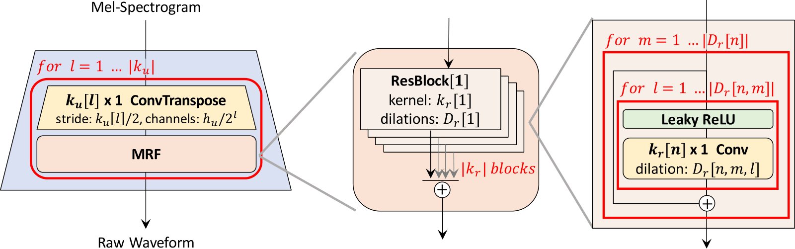
Figure 1: The generator upsamples mel-spectrograms up to times to match the temporal resolution of raw waveforms. A MRF module adds features from residual blocks of different kernel sizes and dilation rates. Lastly, the -th residual block with kernel size and dilation rates in a MRF module is depicted.
图 1:生成器将梅尔频谱上采样至 倍,以匹配原始波形时间分辨率。MRF 模块把 个不同核大小与膨胀率的残差块特征相加。最后画出 MRF 中第 个残差块:核大小 、膨胀率 。
2.3 Discriminator
2.3 判别器
Identifying long-term dependencies is the key for modeling realistic speech audio. For example, a phoneme duration can be longer than 100 ms, resulting in high correlation between more than 2,200 adjacent samples in the raw waveform. This problem has been addressed in the previous work (Donahue et al. 2018) by increasing receptive fields of the generator and discriminator. We focus on another crucial problem that has yet been resolved; as speech audio consists of sinusoidal signals with various periods, the diverse periodic patterns underlying in the audio data need to be identified.
识别长程依赖是建模逼真语音的关键。例如,一个音素可持续超过 100 ms,使原始波形上超过 2,200 个相邻采样高度相关。先前工作(Donahue 等 2018)通过增大生成器与判别器感受野应对这一问题。我们关注另一个尚未充分解决的关键:语音由多种周期正弦成分构成,需要识别数据中多样的周期模式。
To this end, we propose the multi-period discriminator (MPD) consisting of several sub-discriminators each handling a portion of periodic signals of input audio. Additionally, to capture consecutive patterns and long-term dependencies, we use the multi-scale discriminator (MSD) proposed in MelGAN (Kumar et al. 2019), which consecutively evaluates audio samples at different levels. We conducted simple experiments to show the ability of MPD and MSD to capture periodic patterns, and the results can be found in Appendix B.
为此我们提出多周期判别器(MPD):由若干子判别器组成,各自处理输入音频中一部分周期信号。为捕获连续模式与长程依赖,我们沿用 MelGAN(Kumar 等 2019)的多尺度判别器(MSD),在不同层级连续评估音频。附录 B 给出简单实验,展示 MPD 与 MSD 捕获周期模式的能力。
Multi-Period Discriminator
MPD is a mixture of sub-discriminators, each of which only accepts equally spaced samples of an input audio; the space is given as period . The sub-discriminators are designed to capture different implicit structures from each other by looking at different parts of an input audio. We set the periods to [2, 3, 5, 7, 11] to avoid overlaps as much as possible. As shown in Figure 2(b), we first reshape 1D raw audio of length into 2D data of height and width and then apply 2D convolutions to the reshaped data. In every convolutional layer of MPD, we restrict the kernel size in the width axis to be 1 to process the periodic samples independently. Each sub-discriminator is a stack of strided convolutional layers with leaky rectified linear unit (ReLU) activation. Subsequently, weight normalization (Salimans and Kingma 2016) is applied to MPD. By reshaping the input audio into 2D data instead of sampling periodic signals of audio, gradients from MPD can be delivered to all time steps of the input audio.
多周期判别器
MPD 是多个子判别器的混合,每个只接受输入音频上等间距采样;间距即周期 。子判别器通过查看输入的不同部分,彼此捕获不同隐结构。周期设为 [2, 3, 5, 7, 11],尽量减少重叠。如图 2(b),先把长度 的一维原始音频重排为高 、宽 的二维数据,再对其做二维卷积。MPD 每一卷积层在宽度轴上核大小限制为 1,以便独立处理各周期采样。每个子判别器是带泄漏 ReLU 的步幅卷积堆叠,并施加权重归一化(Salimans 与 Kingma 2016)。用重排而非直接抽周期采样,可使 MPD 的梯度传到输入音频的所有时间步。
Multi-Scale Discriminator
Because each sub-discriminator in MPD only accepts disjoint samples, we add MSD to consecutively evaluate the audio sequence. The architecture of MSD is drawn from that of MelGAN (Kumar et al. 2019). MSD is a mixture of three sub-discriminators operating on different input scales: raw audio, 2 average-pooled audio, and 4 average-pooled audio, as shown in Figure 2(a). Each of the sub-discriminators in MSD is a stack of strided and grouped convolutional layers with leaky ReLU activation. The discriminator size is increased by reducing stride and adding more layers. Weight normalization is applied except for the first sub-discriminator, which operates on raw audio. Instead, spectral normalization (Miyato et al. 2018) is applied and stabilizes training as it reported.
多尺度判别器
由于 MPD 各子判别器只看不相交采样,我们加入 MSD 以连续评估音频序列。MSD 结构取自 MelGAN(Kumar 等 2019),由三个子判别器组成,分别作用于不同输入尺度:原始音频、2 平均池化音频、4 平均池化音频,见图 2(a)。各子判别器是带泄漏 ReLU 的步幅与分组卷积堆叠;通过减小步幅、加深层数来增大判别器规模。除作用于原始音频的第一个子判别器外均用权重归一化;第一个改用谱归一化(Miyato 等 2018),据报告可稳定训练。
Note that MPD operates on disjoint samples of raw waveforms, whereas MSD operates on smoothed waveforms.
注意:MPD 作用于原始波形的不相交采样,而 MSD 作用于平滑后的波形。
For previous work using multi-discriminator architecture such as MPD and MSD, Bińkowski et al. 2019’s work can also be referred. The discriminator architecture proposed in the work has resemblance to MPD and MSD in that it is a mixture of discriminators, but MPD and MSD are Markovian window-based fully unconditional discriminator, whereas it averages the output and has conditional discriminators. Also, the resemblance between MPD and RWD (Bińkowski et al. 2019) can be considered in the part of reshaping input audio, but MPD uses periods set to prime numbers to discriminate data of as many periods as possible, whereas RWD uses reshape factors of overlapped periods and does not handle each channel of the reshaped data separately, which are different from what MPD is aimed for. A variation of RWD can perform a similar operation to MPD, but it is also not the same as MPD in terms of parameter sharing and strided convolution to adjacent signals. More details of the architectural difference can be found in Appendix C.
先前也有多判别器结构,如 Bińkowski 等 2019,可对照。其判别器同为多个判别器的混合,与 MPD、MSD 有相似处,但 MPD/MSD 是基于马尔可夫窗的全无条件判别器,而前者对输出取平均并含有条件判别器。MPD 与 RWD(Bińkowski 等 2019)在输入重排上也可对照,但 MPD 用质数周期以尽量覆盖多种周期,而 RWD 的重排因子对应重叠周期,且不单独处理重排后各通道——这与 MPD 的目标不同。RWD 的某种变体可做类似 MPD 的运算,但在参数共享与对相邻信号的步幅卷积上仍不同。更多结构差异见附录 C。
(a)
2.4 Training Loss Terms
2.4 训练损失项
GAN Loss
For brevity, we describe our discriminators, MSD and MPD, as one discriminator throughout Section 2.4. For the generator and discriminator, the training objectives follow LSGAN (Mao et al. 2017), which replace the binary cross-entropy terms of the original GAN objectives (Goodfellow et al. 2014) with least squares loss functions for non-vanishing gradient flows. The discriminator is trained to classify ground truth samples to 1, and the samples synthesized from the generator to 0. The generator is trained to fake the discriminator by updating the sample quality to be classified to a value almost equal to 1. GAN losses for the generator and the discriminator are defined as
GAN 损失
为简洁起见,第 2.4 节把 MSD 与 MPD 统称为一个判别器。生成器与判别器的训练目标沿用 LSGAN(Mao 等 2017),用最小二乘损失替换原始 GAN(Goodfellow 等 2014)中的二元交叉熵,以减轻梯度消失。判别器把真值样本判为 1、生成样本判为 0;生成器则把样本质量抬到接近 1,以骗过判别器。生成器 与判别器 的 GAN 损失定义为
, where denotes the ground truth audio and denotes the input condition, the mel-spectrogram of the ground truth audio.
,其中 为真值音频, 为输入条件,即真值音频的梅尔频谱。
Mel-Spectrogram Loss
In addition to the GAN objective, we add a mel-spectrogram loss to improve the training efficiency of the generator and the fidelity of the generated audio. Referring to previous work (Isola et al. 2017), applying a reconstruction loss to GAN model helps to generate realistic results, and in Yamamoto et al. 2020’s work, time-frequency distribution is effectively captured by jointly optimizing multi-resolution spectrogram and adversarial loss functions. We used mel-spectrogram loss according to the input conditions, which can also be expected to have the effect of focusing more on improving the perceptual quality due to the characteristics of the human auditory system. The mel-spectrogram loss is the L1 distance between the mel-spectrogram of a waveform synthesized by the generator and that of a ground truth waveform. It is defined as
梅尔频谱损失
除 GAN 目标外,我们加入梅尔频谱损失,以提升生成器训练效率与生成音频保真度。参考先前工作(Isola 等 2017),给 GAN 加重建损失有助于生成更真实结果;Yamamoto 等 2020 也表明联合优化多分辨率频谱与对抗损失可有效捕获时频分布。我们按输入条件使用梅尔频谱损失,并期望借助人耳听觉特性更关注感知质量。该损失是生成波形与真值波形梅尔频谱之间的 L1 距离,定义为
, where is the function that transforms a waveform into the corresponding mel-spectrogram. The mel-spectrogram loss helps the generator to synthesize a realistic waveform corresponding to an input condition, and also stabilizes the adversarial training process from the early stages.
,其中 把波形变成对应梅尔频谱。梅尔频谱损失帮助生成器按输入条件合成逼真波形,也从早期就稳定对抗训练。
Feature Matching Loss
The feature matching loss is a learned similarity metric measured by the difference in features of the discriminator between a ground truth sample and a generated sample (Larsen et al. 2016, Kumar et al. 2019). As it was successfully adopted to speech synthesis (Kumar et al. 2019), we use it as an additional loss to train the generator. Every intermediate feature of the discriminator is extracted, and the L1 distance between a ground truth sample and a conditionally generated sample in each feature space is calculated. The feature matching loss is defined as
特征匹配损失
特征匹配损失是一种可学习的相似度度量,由判别器在真值样本与生成样本上的特征差给出(Larsen 等 2016、Kumar 等 2019)。该损失已成功用于语音合成(Kumar 等 2019),我们将其作为生成器的额外损失。提取判别器每一中间特征,在各特征空间计算真值与条件生成样本的 L1 距离。特征匹配损失定义为
, where denotes the number of layers in the discriminator; and denote the features and the number of features in the -th layer of the discriminator, respectively.
,其中 为判别器层数; 与 分别为第 层的特征及其特征数。
Final Loss
Our final objectives for the generator and discriminator are as
最终损失
生成器与判别器的最终目标为
, where we set and . Because our discriminator is a set of sub-discriminators of MPD and MSD, Equations 5 and 6 can be converted with respect to the sub-discriminators as
,其中取 、。由于判别器是 MPD 与 MSD 的子判别器集合,式 5 与 6 可改写为对各子判别器求和:
, where denotes the -th sub-discriminator in MPD and MSD.
,其中 表示 MPD 与 MSD 中的第 个子判别器。
3 Experiments
3 实验
For fair and reproducible comparison with other models, we used the LJSpeech dataset (Ito 2017) in which many speech synthesis models are trained. LJSpeech consists of 13,100 short audio clips of a single speaker with a total length of approximately 24 hours. The audio format is 16-bit PCM with a sample rate of 22 kHz; it was used without any manipulation. HiFi-GAN was compared against the best publicly available models: the popular mixture of logistics (MoL) WaveNet (Oord et al. 2018) implementation (Yamamoto 2018) [^3] and the official implementation of WaveGlow (Valle 2018b) and MelGAN (Kumar 2019). We used the provided pretrained weights for all the models.
为公平、可复现地与其他模型比较,我们使用许多语音合成模型都在其上训练的 LJSpeech 数据集(Ito 2017)。LJSpeech 含单说话人约 13,100 段短音频,总时长约 24 小时;格式为 16-bit PCM、采样率 22 kHz,未做额外处理。对照模型取当时公开最佳:流行的 mixture of logistics(MoL)WaveNet(Oord 等 2018)实现(Yamamoto 2018)[^3],以及 WaveGlow(Valle 2018b)与 MelGAN(Kumar 2019)官方实现。各模型均使用提供的预训练权重。
To evaluate the generality of HiFi-GAN to the mel-spectrogram inversion of unseen speakers, we used the VCTK multi-speaker dataset (Veaux et al. 2017), which consists of approximately 44,200 short audio clips uttered by 109 native English speakers with various accents. The total length of the audio clips is approximately 44 hours. The audio format is 16-bit PCM with a sample rate of 44 kHz. We reduced the sample rate to 22 kHz. We randomly selected nine speakers and excluded all their audio clips from the training set. We then trained MoL WaveNet, WaveGlow, and MelGAN with the same data settings; all the models were trained until 2.5M steps.
为评估对未见说话人梅尔频谱反演的通用性,我们使用 VCTK 多说话人数据集(Veaux 等 2017):约 44,200 段短音频,由 109 位带不同口音的英语母语者录制,总时长约 44 小时;原始 16-bit PCM、44 kHz,我们降到 22 kHz。随机选九位说话人,其全部音频从训练集剔除。再用相同数据设置训练 MoL WaveNet、WaveGlow 与 MelGAN;各模型训至 2.5M 步。
To evaluate the audio quality, we crowd-sourced 5-scale MOS tests via Amazon Mechanical Turk. The MOS scores were recorded with 95% confidence intervals (CI). Raters listened to the test samples randomly, where they were allowed to evaluate each audio sample once. All audio clips were normalized to prevent the influence of audio volume differences on the raters. All quality assessments in Section 4 were conducted in this manner, and were not sourced from other papers.
音质评估通过 Amazon Mechanical Turk 众包 5 分制 MOS;报告带 95% 置信区间(CI)。评分者随机听测样,每段音频只评一次。所有片段归一化,避免音量差影响判断。第 4 节全部质量评估均按此流程,不引用他文数字。
The synthesis speed was measured on GPU and CPU environments according to the recent research trends regarding the efficiency of neural networks (Kumar et al. 2019, Zhai et al. 2020, Tan et al. 2020). The devices used are a single NVIDIA V100 GPU and a MacBook Pro laptop (Intel i7 CPU 2.6GHz). Additionally, we used 32-bit floating point operations for all the models without any optimization methods.
合成速度在 GPU 与 CPU 上测量,以呼应近期对神经网络效率的关注(Kumar 等 2019、Zhai 等 2020、Tan 等 2020)。设备为单块 NVIDIA V100 GPU 与一台 MacBook Pro(Intel i7 CPU 2.6GHz)。各模型均用 32 位浮点运算,不加任何优化技巧。
To confirm the trade-off between synthesis efficiency and sample quality, we conducted experiments based on the three variations of the generator, , , and while maintaining the same discriminator configuration. For , we set , , , and . is simply a smaller version of , which has a smaller hidden dimension but with exactly the same receptive fields. To further reduce the number of layers while maintaining receptive fields wide, the kernel sizes and dilation rates of were selected carefully. The detailed configurations of the models are listed in Appendix A.1. We used 80 bands mel-spectrograms as input conditions. The FFT, window, and hop size were set to 1024, 1024, and 256, respectively. The networks were trained using the AdamW optimizer (Loshchilov and Hutter 2017) with , , and weight decay . The learning rate decay was scheduled by a factor in every epoch with an initial learning rate of .
为确认合成效率与样本质量的权衡,我们在判别器配置不变下,对生成器三个变体 、、 做实验。 取 ,,,。 是更小的 :,感受野完全相同。 则在尽量保持宽感受野的前提下进一步减层,核大小与膨胀率经仔细选取。详细配置见附录 A.1。输入为 80 带梅尔频谱;FFT、窗长、hop 分别为 1024、1024、256。优化器用 AdamW(Loshchilov 与 Hutter 2017),、,权重衰减 。学习率每 epoch 乘 衰减,初始 。
4 Results
4 结果
4.1 Audio Quality and Synthesis Speed
4.1 音质与合成速度
To evaluate the performance of our models in terms of both quality and speed, we performed the MOS test for spectrogram inversion, and the speed measurement. For the MOS test, we randomly selected 50 utterances from the LJSpeech dataset and used the ground truth spectrograms of the utterances which were excluded from training as input conditions.
为同时评估质量与速度,我们对频谱反演做 MOS 测试并测速。MOS 从 LJSpeech 随机抽 50 句,用未参与训练的真值频谱作输入条件。
For easy comparison of audio quality, synthesis speed and model size, the results are compiled and presented in Table1. Remarkably, all variations of HiFi-GAN scored higher than the other models. has 13.92M parameters and achieves the highest MOS with a gap of 0.09 compared to the ground truth audio; this implies that the synthesized audio is nearly indistinguishable from the human voice. In terms of synthesis speed, is faster than WaveGlow and MoL WaveNet. also demonstrates similarity to human quality with a MOS of 4.23 while significantly reducing the memory requirement and inference time, compared to . It only requires 0.92M parameters. Despite having the lowest MOS among our models, can synthesize speech 13.44 times faster than real-time on CPU and 1,186 times faster than real-time on single V100 GPU while showing similar perceptual quality with MoL WaveNet. As efficiently synthesizes speech on CPU, it can be well suited for on-device applications.
音质、合成速度与模型大小汇总见表 1。值得注意的是,HiFi-GAN 各变体均高于其他模型。 有 13.92M 参数,MOS 最高,与真值仅差 0.09,说明合成几乎难以与人声区分。速度上 快于 WaveGlow 与 MoL WaveNet。 MOS 4.23,仍接近真人,相对 大幅降低显存与推理时间,参数仅 0.92M。 在我们模型中 MOS 最低,但 CPU 上相对实时快 13.44 倍、单块 V100 上快 1,186 倍,感知质量与 MoL WaveNet 相近;因能在 CPU 上高效合成,适合端侧应用。
| Model | MOS (CI) | MOS (CI) | Speed on CPU (kHz) | Speed on CPU | (kHz) | Speed on GPU (kHz) | Speed on GPU | (kHz) | # Param (M) | # Param | (M) |
|---|---|---|---|---|---|---|---|---|---|---|---|
| MOS (CI) | |||||||||||
| Speed on CPU | |||||||||||
| (kHz) | |||||||||||
| Speed on GPU | |||||||||||
| (kHz) | |||||||||||
| # Param | |||||||||||
| (M) | |||||||||||
| Ground Truth | 4.45 (0.06) | ||||||||||
| WaveNet (MoL) | 4.02 (0.08) | 0.07 | () | 24.73 | |||||||
| WaveGlow | 3.81 (0.08) | 4.72 | () | 501 | () | 87.73 | |||||
| MelGAN | 3.79 (0.09) | 145.52 | () | 14,238 | () | 4.26 | |||||
| HiFi-GAN | 4.36 (0.07) | 31.74 | (1.43) | 3,701 | (167.86) | 13.92 | |||||
| HiFi-GAN | 4.23 (0.07) | 214.97 | (9.74) | 16,863 | (764.80) | 0.92 | |||||
| HiFi-GAN | 4.05 (0.08) | 296.38 | (13.44) | 26,169 | (1,186.80) | 1.46 |
| MOS (CI) |
|---|
| Speed on CPU |
|---|
| (kHz) |
| Speed on GPU |
|---|
| (kHz) |
| # Param |
|---|
| (M) |
Table 1: Comparison of the MOS and the synthesis speed. Speed of kHz means that the model can generate raw audio samples per second. The numbers in () mean the speed compared to real-time.
| Model | MOS (CI) | Speed on CPU (kHz) | Speed on GPU (kHz) | # Param (M) |
|---|---|---|---|---|
| Ground Truth | 4.45 (0.06) | |||
| WaveNet (MoL) | 4.02 (0.08) | 0.07 () | 24.73 | — |
| WaveGlow | 3.81 (0.08) | 4.72 () | 501 () | 87.73 |
| MelGAN | 3.79 (0.09) | 145.52 () | 14,238 () | 4.26 |
| HiFi-GAN | 4.36 (0.07) | 31.74 (1.43) | 3,701 (167.86) | 13.92 |
| HiFi-GAN | 4.23 (0.07) | 214.97 (9.74) | 16,863 (764.80) | 0.92 |
| HiFi-GAN | 4.05 (0.08) | 296.38 (13.44) | 26,169 (1,186.80) | 1.46 |
表 1:MOS 与合成速度对比。速度 kHz 表示每秒可生成 个原始音频采样。括号内为相对实时的倍数。
4.2 Ablation Study
4.2 消融实验
We performed an ablation study of MPD, MRF, and mel-spectrogram loss to verify the effect of each HiFi-GAN component on the quality of the synthesized audio. that has the smallest expressive power among the three generator variations was used as a generator for the ablation study, and the network parameters were updated up to 500k steps for each configuration.
我们对 MPD、MRF 与梅尔频谱损失做消融,验证各组件对合成音质的影响。生成器取三个变体中表达能力最小的 ,每种配置更新至 500k 步。
The results of the MOS evaluation are shown in Table 2, which show all three components contribute to the performance. Removing MPD causes a significant decrease in perceptual quality, whereas the absence of MSD shows a relatively small but noticeable degradation. To investigate the effect of MRF, one residual block with the widest receptive field was retained in each MRF module. The result is also worse than the baseline. The experiment on the mel-spectrogram loss shows that it helps improve the quality, and we observed that the quality improves more stably when the loss is applied.
MOS 见表 2,三项均有贡献。去掉 MPD 感知质量大幅下降;去掉 MSD 也有可见但相对较小的劣化。为考察 MRF,每个 MRF 只保留感受野最宽的一个残差块,结果仍差于基线。梅尔频谱损失的实验表明它有助于提质,且我们观察到加该项后质量提升更稳。
To verify the effect of MPD in the settings of other GAN models, we introduced MPD in MelGAN. MelGAN trained with MPD outperforms the original one by a gap of 0.47 MOS, which shows statistically significant improvement.
为验证 MPD 在其他 GAN 设定中的作用,我们把 MPD 引入 MelGAN。带 MPD 的 MelGAN 比原版高 0.47 MOS,提升具有统计显著性。
We experimented with periods of powers of 2 to verify the effect of periods set to prime numbers. While the period 2 allows signals to be processed closely, it results in statistically significant degradation with a difference of 0.20 MOS from the baseline.
我们还试过 2 的幂次周期,以对照质数周期。周期 2 虽使信号处理更「密」,但相对基线差 0.20 MOS,劣化具有统计显著性。
| Model | MOS (CI) |
|---|---|
| Ground Truth | 4.57 (0.04) |
| Baseline (HiFi-GAN ) | 4.10 (0.05) |
| w/o MPD | 2.28 (0.09) |
| w/o MSD | 3.74 (0.05) |
| w/o MRF | 3.92 (0.05) |
| w/o Mel-Spectrogram Loss | 3.25 (0.05) |
| MPD =[2,4,8,16,32] | 3.90 (0.05) |
| MelGAN | 2.88 (0.08) |
| MelGAN with MPD | 3.35 (0.07) |
Table 2: Ablation study results. Comparison of the effect of each component on the synthesis quality.
| Model | MOS (CI) |
|---|---|
| Ground Truth | 4.57 (0.04) |
| Baseline (HiFi-GAN ) | 4.10 (0.05) |
| w/o MPD | 2.28 (0.09) |
| w/o MSD | 3.74 (0.05) |
| w/o MRF | 3.92 (0.05) |
| w/o Mel-Spectrogram Loss | 3.25 (0.05) |
| MPD =[2,4,8,16,32] | 3.90 (0.05) |
| MelGAN | 2.88 (0.08) |
| MelGAN with MPD | 3.35 (0.07) |
表 2:消融结果。各组件对合成质量的影响对比。
4.3 Generalization to Unseen Speakers
4.3 推广到未见说话人
We used 50 randomly selected utterances of nine unseen speakers in the VCTK dataset that were excluded from the training set for the MOS test. Table 4 shows the experimental results for the mel-spectrogram inversion of the unseen speakers. The three generator variations scored 3.77, 3.69, and 3.61. They were all better than AR and flow-based models, indicating that the proposed models generalize well to unseen speakers. Additionally, the tendency of difference in MOS scores of the proposed models is similar with the result shown in Section 4.1, which exhibits generalization across different datasets.
从训练时剔除的九位未见说话人中,随机抽 50 句做 MOS。表 3 给出未见说话人梅尔频谱反演结果。三个生成器变体得分 3.77、3.69、3.61,均优于 AR 与流模型,表明对未见说话人推广良好。各变体 MOS 差距趋势也与第 4.1 节相近,说明跨数据集表现一致。
| Model | MOS (CI) |
|---|---|
| Ground Truth | 3.79 (0.07) |
| WaveNet (MoL) | 3.52 (0.08) |
| WaveGlow | 3.52 (0.08) |
| MelGAN | 3.50 (0.08) |
| HiFi-GAN | 3.77 (0.07) |
| HiFi-GAN | 3.69 (0.07) |
| HiFi-GAN | 3.61 (0.07) |
| Model | MOS (CI) |
|---|---|
| Ground Truth | 4.23 (0.07) |
| WaveGlow (w/o fine-tuning) | 3.69 (0.08) |
| HiFi-GAN (w/o fine-tuning) | 3.91 (0.08) |
| HiFi-GAN (w/o fine-tuning) | 3.88 (0.08) |
| HiFi-GAN (w/o fine-tuning) | 3.89 (0.08) |
| WaveGlow (find-tuned) | 3.66 (0.08) |
| HiFi-GAN (find-tuned) | 4.18 (0.08) |
| HiFi-GAN (find-tuned) | 4.12 (0.07) |
| HiFi-GAN (find-tuned) | 4.02 (0.08) |
Table 3: Quality comparison of synthesized utterances for unseen speakers.
| Model | MOS (CI) |
|---|---|
| Ground Truth | 3.79 (0.07) |
| WaveNet (MoL) | 3.52 (0.08) |
| WaveGlow | 3.52 (0.08) |
| MelGAN | 3.50 (0.08) |
| HiFi-GAN | 3.77 (0.07) |
| HiFi-GAN | 3.69 (0.07) |
| HiFi-GAN | 3.61 (0.07) |
| Model | MOS (CI) |
|---|---|
| Ground Truth | 4.23 (0.07) |
| WaveGlow (w/o fine-tuning) | 3.69 (0.08) |
| HiFi-GAN (w/o fine-tuning) | 3.91 (0.08) |
| HiFi-GAN (w/o fine-tuning) | 3.88 (0.08) |
| HiFi-GAN (w/o fine-tuning) | 3.89 (0.08) |
| WaveGlow (fine-tuned) | 3.66 (0.08) |
| HiFi-GAN (fine-tuned) | 4.18 (0.08) |
| HiFi-GAN (fine-tuned) | 4.12 (0.07) |
| HiFi-GAN (fine-tuned) | 4.02 (0.08) |
表 3:未见说话人合成语句的质量对比。
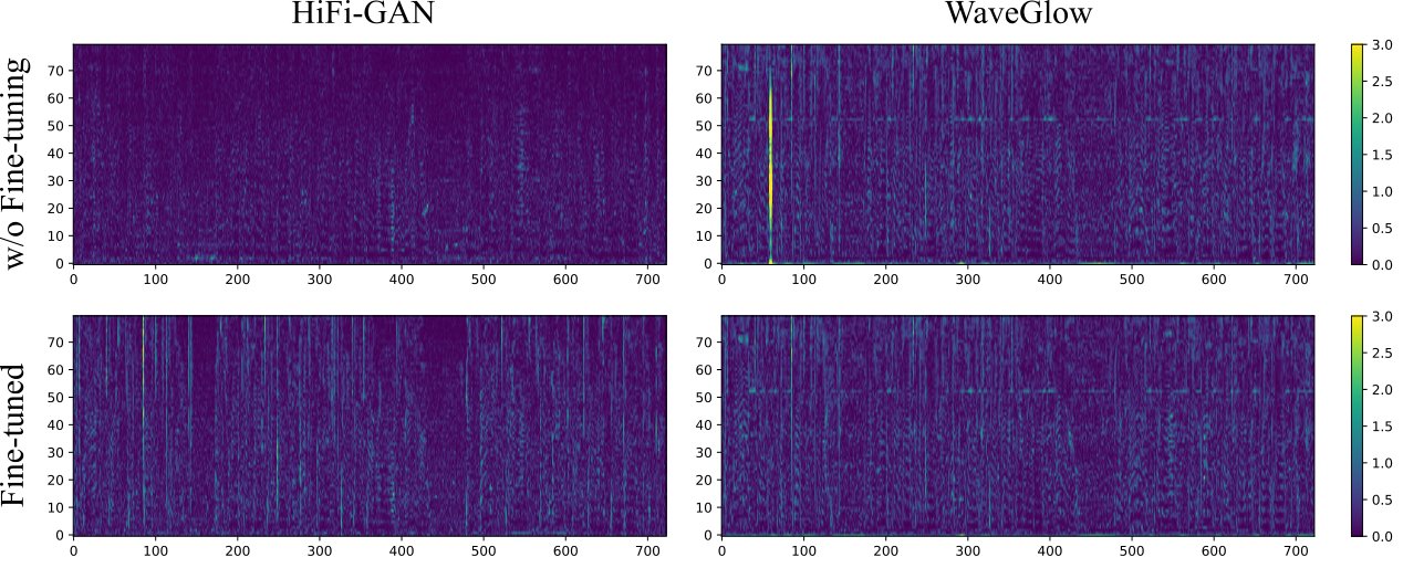
Figure 3: Pixel-wise difference in the mel-spectrogram domain between generated waveforms and a mel-spectrogram from Tacotron2. Before fine-tuning, HiFi-GAN generates waveforms corresponding to input conditions accurately. After fine-tuning, the error of the mel-spectrogram level increased, but the perceptual quality increased.
图 3:生成波形与 Tacotron2 梅尔频谱在梅尔域的逐像素差。微调前,HiFi-GAN 能准确对应输入条件;微调后梅尔级误差上升,但感知质量提升。
4.4 End-to-End Speech Synthesis
4.4 端到端语音合成
We conducted an additional experiment to examine the effectiveness of the proposed models when applied to an end-to-end speech synthesis pipeline, which consists of text to mel-spectrogram and mel-spectrogram to waveform synthesis modules. We herein used Tacotron2 (Shen et al. 2018) to generate mel-spectrograms from text. Without any modification, we synthesized the mel-spectrograms using the most popular implementation of Tacotron2 (Valle 2018a) with the provided pre-trained weights. We then fed them as input conditions into second stage models, including our models and WaveGlow used in Section 4.1.[^4]
我们另做实验,考察模型接在端到端流水线(文本到梅尔频谱 再 梅尔频谱到波形)中的效果。用 Tacotron2(Shen 等 2018)从文本生成梅尔频谱;不做改动,采用最流行的 Tacotron2 实现(Valle 2018a)及提供的预训练权重,再把频谱喂给第 4.1 节中的第二阶段模型(含我们的模型与 WaveGlow)。[^4]
The MOS scores are listed in Table 4. The results without fine-tuning show that all the proposed models outperform WaveGlow in the end-to-end setting, while the audio quality of all models are unsatisfactory compared to the ground truth audio. However, when the pixel-wise difference in the mel-spectrogram domain between generated waveforms and a mel-spectrogram from Tacotron2 are investigated as demonstrated in Figure 3, we found that the difference is insignificant, which means that the predicted mel-spectrogram from Tacotron2 was already noisy. To improve the audio quality in the end-to-end setting, we applied fine-tuning with predicted mel-spectrograms of Tacotron2 in teacher-forcing mode (Shen et al. 2018) to all the models up to 100k steps. MOS scores of all the fine-tuned proposed models over 4, whereas fine-tuned WaveGlow did not show quality improvement. We conclude that HiFi-GAN adapts well on the end-to-end setting with fine-tuning.
MOS 见表 4。未微调时,各提出模型在端到端设定下均优于 WaveGlow,但相对真值仍不够满意。观察生成波形与 Tacotron2 频谱在梅尔域的逐像素差(图 3)发现,差值其实不大——说明 Tacotron2 预测的频谱本身已偏噪。为提升端到端音质,我们用 Tacotron2 在教师强制模式(Shen 等 2018)下的预测梅尔频谱,对各模型微调至 100k 步。微调后提出模型 MOS 均超过 4,而微调 WaveGlow 未见提升。结论是:经微调后,HiFi-GAN 能很好适应端到端设定。
5 Conclusion
5 结论
In this work, we introduced HiFi-GAN, which can efficiently synthesize high quality speech audio. Above all, our proposed model outperforms the best performing publicly available models in terms of synthesis quality, even comparable to human level. Moreover, it shows a significant improvement in terms of synthesis speed. We took inspiration from the characteristic of speech audio that consists of patterns with various periods and applied it to neural networks, and verified that the existence of the proposed discriminator greatly influences the quality of speech synthesis through the ablation study. Additionally, this work presents several experiments that are significant in speech synthesis applications. HiFi-GAN shows ability to generalize unseen speakers and synthesize speech audio comparable to human quality from noisy inputs in an end-to-end setting. In addition, our small footprint model demonstrates comparable sample quality with the best publicly available autoregressive counterpart, while generating samples in an order-of-magnitude faster than real-time on CPU. This shows progress towards on-device natural speech synthesis, which requires low latency and memory footprint. Finally, our experiments show that the generators of various configurations can be trained with the same discriminators and learning mechanism, which indicates the possibility of flexibly selecting a generator configuration according to the target specifications without the need for a time-consuming hyper-parameter search for the discriminators. We release HiFi-GAN as open source. We envisage that our work will serve as a basis for future speech synthesis studies.
本文提出能高效合成高质量语音的 HiFi-GAN。首先,合成质量优于当时公开最佳模型,甚至可与人声接近;其次,合成速度显著提升。我们从「语音由多种周期模式构成」这一特点出发,把它落到网络结构上,并通过消融验证所提判别器对合成质量影响巨大。文中若干实验对应用也很关键:HiFi-GAN 能推广到未见说话人,并在端到端、带噪输入下合成接近真人的语音;小体积版本质量可与公开最佳自回归对照相比,却在 CPU 上比实时快一个数量级,朝低延迟、低占用的端侧自然语音合成迈进一步。实验还表明,同一套判别器与学习机制可训练多种生成器配置,因而可按目标规格灵活选型,而不必为判别器做耗时的超参搜索。HiFi-GAN 已开源,希望能为后续语音合成研究提供基础。
Acknowledgments
致谢
We would like to thank Bokyung Son, Sungwon Kim, Yongjin Cho and Sungwon Lyu.
感谢 Bokyung Son、Sungwon Kim、Yongjin Cho 与 Sungwon Lyu。
References
参考文献
Bińkowski et al. (2019) Mikołaj Bińkowski, Jeff Donahue, Sander Dieleman, Aidan Clark, Erich Elsen, Norman Casagrande, Luis C Cobo, and Karen Simonyan. High fidelity speech synthesis with adversarial networks. arXiv preprint arXiv:1909.11646 , 2019.
Donahue et al. (2018) Chris Donahue, Julian McAuley, and Miller Puckette. Adversarial audio synthesis. arXiv preprint arXiv:1802.04208 , 2018.
Goodfellow et al. (2014) Ian Goodfellow, Jean Pouget-Abadie, Mehdi Mirza, Bing Xu, David Warde-Farley, Sherjil Ozair, Aaron Courville, and Yoshua Bengio. Generative adversarial nets. In Advances in neural information processing systems , pages 2672–2680, 2014.
Isola et al. (2017) Phillip Isola, Jun-Yan Zhu, Tinghui Zhou, and Alexei A Efros. Image-to-image translation with conditional adversarial networks. In Proceedings of the IEEE conference on computer vision and pattern recognition , pages 1125–1134, 2017.
Ito (2017) Keith Ito. The lj speech dataset. https://keithito.com/LJ-Speech-Dataset/ , 2017.
Kingma and Dhariwal (2018) Durk P Kingma and Prafulla Dhariwal. Glow: Generative flow with invertible 1x1 convolutions. In Advances in Neural Information Processing Systems , pages 10215–10224, 2018.
Kumar et al. (2019) Kundan Kumar, Rithesh Kumar, Thibault de Boissiere, Lucas Gestin, Wei Zhen Teoh, Jose Sotelo, Alexandre de Brébisson, Yoshua Bengio, and Aaron C Courville. Melgan: Generative adversarial networks for conditional waveform synthesis. In Advances in Neural Information Processing Systems 32 , pages 14910–14921, 2019.
Kumar (2019) Rithesh Kumar. descriptinc/melgan-neurips. https://github.com/descriptinc/melgan-neurips , 2019.
Larsen et al. (2016) Anders Boesen Lindbo Larsen, Søren Kaae Sønderby, Hugo Larochelle, and Ole Winther. Autoencoding beyond pixels using a learned similarity metric. In International conference on machine learning , pages 1558–1566. PMLR, 2016.
Li et al. (2019) Naihan Li, Shujie Liu, Yanqing Liu, Sheng Zhao, and Ming Liu. Neural speech synthesis with transformer network. In Proceedings of the AAAI Conference on Artificial Intelligence , volume 33, pages 6706–6713, 2019.
Loshchilov and Hutter (2017) Ilya Loshchilov and Frank Hutter. Decoupled weight decay regularization. arXiv preprint arXiv:1711.05101 , 2017.
Mao et al. (2017) Xudong Mao, Qing Li, Haoran Xie, Raymond YK Lau, Zhen Wang, and Stephen Paul Smolley. Least squares generative adversarial networks. In Proceedings of the IEEE International Conference on Computer Vision , pages 2794–2802, 2017.
Mathieu et al. (2015) Michael Mathieu, Camille Couprie, and Yann LeCun. Deep multi-scale video prediction beyond mean square error. arXiv preprint arXiv:1511.05440 , 2015.
Miyato et al. (2018) Takeru Miyato, Toshiki Kataoka, Masanori Koyama, and Yuichi Yoshida. Spectral normalization for generative adversarial networks. arXiv preprint arXiv:1802.05957 , 2018.
Oord et al. (2018) Aaron Oord, Yazhe Li, Igor Babuschkin, Karen Simonyan, Oriol Vinyals, Koray Kavukcuoglu, George Driessche, Edward Lockhart, Luis Cobo, Florian Stimberg, et al. Parallel wavenet: Fast high-fidelity speech synthesis. In International conference on machine learning , pages 3918–3926. PMLR, 2018.
Oord et al. (2016) Aaron van den Oord, Sander Dieleman, Heiga Zen, Karen Simonyan, Oriol Vinyals, Alex Graves, Nal Kalchbrenner, Andrew Senior, and Koray Kavukcuoglu. Wavenet: A generative model for raw audio. arXiv preprint arXiv:1609.03499 , 2016.
Ping et al. (2017) Wei Ping, Kainan Peng, Andrew Gibiansky, Sercan O Arik, Ajay Kannan, Sharan Narang, Jonathan Raiman, and John Miller. Deep voice 3: Scaling text-to-speech with convolutional sequence learning. arXiv preprint arXiv:1710.07654 , 2017.
Ping et al. (2018) Wei Ping, Kainan Peng, and Jitong Chen. Clarinet: Parallel wave generation in end-to-end text-to-speech. arXiv preprint arXiv:1807.07281 , 2018.
Prenger et al. (2019) Ryan Prenger, Rafael Valle, and Bryan Catanzaro. Waveglow: A flow-based generative network for speech synthesis. In ICASSP 2019-2019 IEEE International Conference on Acoustics, Speech and Signal Processing (ICASSP) , pages 3617–3621. IEEE, 2019.
Salimans and Kingma (2016) Tim Salimans and Durk P Kingma. Weight normalization: A simple reparameterization to accelerate training of deep neural networks. In Advances in neural information processing systems , pages 901–909, 2016.
Shen et al. (2018) Jonathan Shen, Ruoming Pang, Ron J Weiss, Mike Schuster, Navdeep Jaitly, Zongheng Yang, Zhifeng Chen, Yu Zhang, Yuxuan Wang, Rj Skerrv-Ryan, et al. Natural tts synthesis by conditioning wavenet on mel spectrogram predictions. In 2018 IEEE International Conference on Acoustics, Speech and Signal Processing (ICASSP) , pages 4779–4783. IEEE, 2018.
Tan et al. (2020) Mingxing Tan, Ruoming Pang, and Quoc V Le. Efficientdet: Scalable and efficient object detection. In Proceedings of the IEEE/CVF Conference on Computer Vision and Pattern Recognition , pages 10781–10790, 2020.
Valle (2018a) Rafael Valle. Nvidia/tacotron2. https://github.com/NVIDIA/tacotron2 , 2018a.
Valle (2018b) Rafael Valle. Nvidia/waveglow. https://github.com/NVIDIA/waveglow , 2018b.
Veaux et al. (2017) Christophe Veaux, Junichi Yamagishi, Kirsten MacDonald, et al. Cstr vctk corpus: English multi-speaker corpus for cstr voice cloning toolkit. University of Edinburgh. The Centre for Speech Technology Research (CSTR) , 2017.
Yamamoto (2018) Ryuichi Yamamoto. wavenet vocoder. https://github.com/r9y9/wavenet_vocoder/ , 2018.
Yamamoto et al. (2020) Ryuichi Yamamoto, Eunwoo Song, and Jae-Min Kim. Parallel wavegan: A fast waveform generation model based on generative adversarial networks with multi-resolution spectrogram. In ICASSP 2020-2020 IEEE International Conference on Acoustics, Speech and Signal Processing (ICASSP) , pages 6199–6203. IEEE, 2020.
Zhai et al. (2020) Bohan Zhai, Tianren Gao, Flora Xue, Daniel Rothchild, Bichen Wu, Joseph E Gonzalez, and Kurt Keutzer. Squeezewave: Extremely lightweight vocoders for on-device speech synthesis. arXiv preprint arXiv:2001.05685 , 2020.
Appendix A
附录 A
A.1. Details of the Model Architecture
A.1. 模型结构细节
The detailed architecture of the generator and MPD is depicted in Figure 4. The configuration of three variants of the generator is listed in Table 5.
生成器与 MPD 的详细结构见图 4。三种生成器变体配置见表 5。
(a)
| Hyper-Parameters | ||||
|---|---|---|---|---|
| Model | ||||
| 512 | [16, 16, 4, 4] | [3, 7, 11] | [[1, 1], [3, 1], [5, 1]] 3 | |
| 128 | [16, 16, 4, 4] | [3, 7, 11] | [[1, 1], [3, 1], [5, 1]] 3 | |
| 256 | [16, 16, 8] | [3, 5, 7] | [[1], [2]], [[2], [6]], [[3], [12]] |
Table 5: Hyper-parameters of three generator , , and .
| Hyper-Parameters | ||||
|---|---|---|---|---|
| Model | ||||
| 512 | [16, 16, 4, 4] | [3, 7, 11] | [[1, 1], [3, 1], [5, 1]] 3 | |
| 128 | [16, 16, 4, 4] | [3, 7, 11] | [[1, 1], [3, 1], [5, 1]] 3 | |
| 256 | [16, 16, 8] | [3, 5, 7] | [[1], [2]], [[2], [6]], [[3], [12]] |
表 5:三种生成器 、、 的超参数。
Each ResBlock in the generators is a structure in which multiple convolution layers and residual connections are stacked. In the ResBlock of V1 and V2, 2 convolution layers and 1 residual connection are stacked 3 times. In the Resblock of V3, 1 convolution layer and 1 residual connection are stacked 2 times. Therefore, V3 consists of a much smaller number of layers than V1 and V2.
生成器中每个 ResBlock 由多层卷积与残差连接堆叠而成。V1 与 V2 的 ResBlock 中,2 层卷积加 1 条残差连接重复堆叠 3 次;V3 的 ResBlock 中,1 层卷积加 1 条残差连接堆叠 2 次。因此 V3 的层数远少于 V1 与 V2。
Appendix B
附录 B
B.1. Periodic signal discrimination experiments
B.1. 周期信号判别实验
We conducted additional experiments similar to training a discriminator using a simple dataset to verify the ability of MPD to discriminate periodic signals. We have assumed that most of the signals generated by the generator are well made, with a very small amount of error signals. We generated 40,000 sinusoidal data of randomly selected frequency in the range of 1~8,000Hz, random phase and random energy. We experimented with 3 ratios to see the performance change according to the difference between the ratio of true and false label. We gave true label [99, 99.5, 99.9]% of the frequencies and false label the remaining frequencies. We added a projection layer to MPD and MSD, trained with these datasets, and compared the classification results of 8,000 unseen data. As this is binary classification, we set the ratio of true label to false label of validation data to 50:50 to facilitate comparison. We repeated this experiment 5 times to get the average, and the results are listed in Table 6. The results show that MPD is superior in discriminating periodic signals than MSD. And remarkably MPD can discriminate 0.1% of false frequencies with 85% accuracy.
我们用简单数据集做额外实验,验证 MPD 判别周期信号的能力。假设生成器产出的多数信号已经不错,只有极少量误差信号。随机在 1~8,000Hz 选频率,并随机相位与能量,生成 40,000 条正弦数据。用三种真/假标签比例观察表现变化:对 [99, 99.5, 99.9]% 的频率给真标签,其余给假标签。给 MPD 与 MSD 加投影层,在这些数据上训练,并在 8,000 条未见数据上比较分类结果。因是二分类,验证集真假比例设为 50:50 便于比较。实验重复 5 次取平均,见表 6。结果显示 MPD 对周期信号的判别优于 MSD;尤为突出的是,MPD 能以约 85% 准确率识别仅占 0.1% 的假频率。
| True Label Ratio | |||
|---|---|---|---|
| Model | 99.0% | 99.5% | 99.9% |
| MSD | 80.76% | 59.01% | 50.42% |
| MPD | 97.01% | 96.38% | 85.33% |
Table 6: Comparison of classification accuracy for periodic signals.
| True Label Ratio | |||
|---|---|---|---|
| Model | 99.0% | 99.5% | 99.9% |
| MSD | 80.76% | 59.01% | 50.42% |
| MPD | 97.01% | 96.38% | 85.33% |
表 6:周期信号分类准确率对比。
B.2. Frequency response analysis of input signals of discriminators
B.2. 判别器输入信号的频率响应分析
(a)
We investigated the importance of modeling discriminators to capture periodic patterns through a toy example. In this example, we train two generators to mimic the sinc function each with MPD and MSD, respectively. we set the domain of sinc function to evenly spaced 1,000 numbers over an interval [-200, 200], and set the function values as the ground-truth signal, which is visualized in Figure 5(a). To maintain the equal structure of MSD and MPD, we set the periods of MPD to [1, 2, 4]. All sub-discriminators of MPD and MSD are designed as feed-forward networks with the same structure. The generator is simply modeled with 1,000 parameters each corresponded to one point of the domain of the ground-truth signal.
我们用玩具例子考察判别器对周期模式建模的重要性。分别用 MPD 与 MSD 训练两个生成器去拟合 sinc 函数。sinc 的定义域取区间 [-200, 200] 上均匀 1,000 个点,函数值作为真值信号,见图 5(a)。为使 MSD 与 MPD 结构对等,MPD 周期取 [1, 2, 4]。MPD 与 MSD 的各子判别器均为同结构前馈网络。生成器仅用 1,000 个参数,各对应真值信号定义域上的一点。

Figure 5(b) shows input signals of sub-discriminators and the magnitude of their frequency responses. In the case of MPD, the frequency responses of input signals are not distorted except for aliasing. On the other hand, the input signals of MSD are getting smoother whenever down-sampling. It is due to the low-pass filtering of average pooling, which results into diminishing amplitudes in high frequencies.
图 5(b) 给出各子判别器输入信号及其频率响应幅度。对 MPD,除混叠外频率响应无明显畸变;对 MSD,每经一次下采样输入更平滑,这是平均池化低通滤波所致,高频幅度被削弱。
When comparing the outputs of learned generators, the difference is more evident. Figure 5(c) shows the outputs of generators each of which is trained with MSD and MPD, respectively. In the case of MPD, the synthesized signal is similar to the ground truth, while in the case of MSD, the synthesized signal is noisy.
比较学到的生成器输出时,差别更明显。图 5(c) 分别给出用 MSD、MPD 训练的生成器输出:MPD 合成接近真值,MSD 则偏噪。
The reason of the sub-optimal outcomes of MSD can be found in average pooling of the down-sampling procedure. Figure 5(d) shows the down-sampled synthesized signals for sub-discriminators and the magnitude of their frequency responses. When it comes to down-sampling synthesized signals for the second and third sub-discriminators of MSD, the result seems similar to that of the ground-truth signal. It indicates that even though there is huge difference between the ground-truth and generated signals, the average-pooled input signals of some sub-discriminators of MSD can be similar. On the other hand, MPD shows similar results to the ground truth regardless of down-sampling factors. In conclusion, we can see that MPD captures more periodic patterns of an input signal than MSD, and capturing periodic patterns is important to model signals.
MSD 效果欠佳的原因可追溯到下采样中的平均池化。图 5(d) 给出供子判别器使用的下采样合成信号及其频率响应幅度。对 MSD 第二、第三子判别器,下采样后的合成信号看起来已接近真值——即便原始真值与生成信号差很大,经平均池化后部分子判别器输入仍可能相近。MPD 则不论下采样因子如何,结果都接近真值。综上,MPD 比 MSD 更能捕获输入的周期模式,而捕获周期模式对建模信号很重要。
Appendix C
附录 C
C.1. Details of architectural difference between RWD and MPD
C.1. RWD 与 MPD 的结构差异细节
When the first layer of RWD is the grouped 1d convolution, the convolution layer of RWD becomes similar to the first 2d convolution with k1 kernels of MPD, but there is still a difference as RWD would not share weights across each group. Moreover, RWD operates on an entire input sequence regardless of input reshaping, while MPD only operates on down-sampled, or evenly spaced, samples from the input sequence. In that regard, it can be seen that RWD uses additional parameters to mix representations of down-sampled samples at each layer, in other words, MPD shares more parameters at each layer than RWD.
若 RWD 第一层是分组一维卷积,则其卷积层会类似 MPD 中核为 k1 的首层二维卷积,但仍有差别:RWD 不会跨组共享权重。此外,无论是否重排,RWD 都对整段输入序列运算;MPD 只对输入中等间距(下采样)采样运算。由此可认为 RWD 在每层额外用参数混合各下采样表示,换言之 MPD 在每层共享的参数更多。