Heat Kernel Textures: the Geodesic Gaussians That Do Not Splat
Heat Kernel Textures: the Geodesic Gaussians That Do Not Splat
Heat Kernel Textures:并不做溅射的测地高斯
Imperial College London
Equal contribution
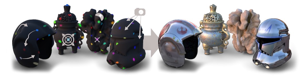
Fig. 1: HKTex: an intrinsic, UV-free texture representation using heat kernels. Left: A Riemannian framework constrains kernel movement to the surface, followed by manifold-aware controllers that manage kernel shape and density. Evaluation occurs within a differentiable ray-tracing pipeline. Right: Final physically based renders.
图 1:HKTex:一种使用热核的内蕴、无需 UV 的纹理表示。左:黎曼框架把核的移动约束在表面上,随后由感知流形的控制器管理核的形状与密度。求值在可微光线追踪流水线中完成。右:最终的基于物理的渲染结果。
Abstract
摘要
3D Gaussian Splatting has recently revolutionised novel view synthesis as well as many other 3D vision methods and applications. Drawing inspiration from this representation, we now rethink textures to overcome the main issues of UV mapping while considerably lowering their memory footprint. Heat Kernel Textures (HKTex) eliminate UV unwrapping as well as their persistent issues of wasted UV space, seams, distortions, vertex-duplication, and varying resolution. Grounded in discrete Riemannian geometry and intrinsically defined on any manifold surface discretised as a triangular mesh, HKTex uses anisotropic heat kernels as geodesic equivalents to Gaussians. Like our kernels, also the optimisation of their position and the adaptive densification strategies were redefined to operate on the surface of the object to be textureised. Our novel representation is also fully integrated with a physically based renderer and can be optimised either from existing textures or multi-view images. Our project page and code are available at circle-group.github.io/research/HeatKernelTextures.
3D Gaussian Splatting 近来不仅改变了新视角合成,也影响了许多其他三维视觉方法与应用。受这一表示启发,我们重新思考纹理,希望克服 UV 映射的主要问题,同时显著降低其内存占用。Heat Kernel Textures(HKTex)不再做 UV 展开,也就避开了 UV 空间浪费、接缝、变形、顶点复制和分辨率不均这些长期存在的问题。它建立在离散黎曼几何之上,内蕴地定义在任何被离散成三角网格的流形表面上,并用各向异性热核作为高斯的测地对应物。与这些核本身一样,位置优化以及自适应加密策略也被重新定义,全部在待纹理化物体的表面上完成。这一新表示还完整接入了基于物理的渲染器,既可以从已有纹理优化,也可以从多视图图像优化。项目页与代码见 circle-group.github.io/research/HeatKernelTextures。
Keywords: Gaussian Splatting · Heat Kernel · Texture · Geodesic
关键词:Gaussian Splatting · 热核 · 纹理 · 测地
1 Introduction
1 引言
Rendering and representation techniques have evolved exponentially over the past decades, but the representation of objects' appearance is still mostly anchored in the traditional and fundamentally flawed UV-mapping. With this representation, points on the surface of a mesh are mapped onto image planes where appearance properties are stored. Not only does this cause visual artifacts like seams, varying resolutions, and distortions, but it also incurs additional storage costs for saving the UV-coordinates associated with every vertex of a mesh and for duplicating vertices on seam lines. Empty UV-mapped regions further exacerbate memory waste. To overcome these limitations, we advocate for a new representation intrinsically defined on the surface of the objects and capable of lowering the memory footprint, with the potential to benefit games, virtual and augmented reality, and visual effects.
过去几十年,渲染与表示技术发展很快,但物体外观的表示大多仍锚定在传统且存在根本缺陷的 UV 映射上。在这种表示里,网格表面上的点被映射到图像平面,外观属性就存放在那里。这样做不仅会造成接缝、分辨率不均和变形这类视觉伪影,还要为网格的每个顶点额外保存 UV 坐标,并在接缝线上复制顶点。空白的 UV 映射区域会进一步加重内存浪费。为克服这些限制,我们主张采用一种内蕴地定义在物体表面上、并能降低内存占用的新表示,它有望用于游戏、虚拟与增强现实以及视觉特效。
Multiple works have attempted to mitigate UV-related issues, most notably through implicit neural representations [19,26] or coloured point clouds [12,45,46]. While promising, these approaches respectively incur considerable memory footprints, present topology-dependent structures, or require a substantial number of primitives. More recently, 3D Gaussian Splatting (3DGS) [18] has revolutionised novel view synthesis through a representation that tightly entangles geometry and appearance. However, standard 3DGS operates entirely in ambient Euclidean space. When applied to surface texturing, this assumption becomes a fundamental flaw: Euclidean optimisation naturally detaches Gaussians from the geometry, and the rigid 3D Gaussians themselves are incapable of bending to conform to the underlying manifold. While recent methods [8,14] attempt to align Gaussians to the surface through the introduction of additional regularisation losses, the fundamental disconnect remains.
已有不少工作试图缓解与 UV 相关的问题,最常见的是隐式神经表示 [19,26],或带颜色的点云 [12,45,46]。这些方法虽有潜力,但分别会带来可观的内存占用、依赖拓扑的结构,或需要大量基元。近来,3D Gaussian Splatting(3DGS)[18] 用一种把几何和外观紧紧缠在一起的表示,改变了新视角合成。不过,标准 3DGS 完全工作在环境欧氏空间中。一旦用来给表面贴纹理,这一假设就成了根本缺陷:欧氏优化会自然地把高斯从几何上拉开,而刚性的三维高斯本身也无法弯曲以贴合底层流形。尽管近期方法 [8,14] 试图靠额外的正则损失把高斯对齐到表面,这种根本上的脱节仍然存在。
In contrast, we introduce a truly intrinsic, geodesic representation where the texturing primitives natively conform to the existing geometry of a mesh. Instead of operating in ambient 3D space, we replace Euclidean Gaussians with anisotropic heat kernels, defining all operations directly on the manifold surface. Specifically, kernel positions are updated through Riemannian geodesic optimisation, and our adaptive density controls also respect the manifold using the exponential map during kernel splits. To continuously and efficiently evaluate kernels across the surface, we devise new techniques to parametrise kernel anisotropies while simultaneously bridging continuous and discrete heat diffusion formulations. Our formulation enables seamless integration into physically based rendering pipelines where our textures can be differentiably ray-traced. It is important to note that our heat kernels are not splatted, but rather dynamically evaluated at ray intersections occurring during rendering. Without loss of generality, we focus this study on albedo texture properties, thus modelling how light reflects. We prove that Heat Kernel Textures (HKTex) can compress existing UV textures and also be used for inverse rendering from 2D photos, thus enabling distortion- and seam-free texture acquisition by construction.
与此相对,我们引入一种真正内蕴的测地表示,其纹理基元天生贴合网格已有的几何。我们不再在环境三维空间中操作,而是用各向异性热核替换欧氏高斯,把全部运算直接定义在流形表面上。具体而言,核的位置通过黎曼测地优化来更新;自适应密度控制在核分裂时也借助指数映射,从而尊重流形。为了在整个表面上连续且高效地求值,我们设计了新的技术来参数化核的各向异性,同时沟通连续与离散的热扩散表述。这一表述可以无缝接入基于物理的渲染流水线,使我们的纹理能够被可微地光线追踪。需要强调的是,我们的热核并不做溅射,而是在渲染过程中于光线交点处动态求值。在不损失一般性的前提下,本研究聚焦于反照率纹理属性,也就是对光如何反射建模。我们证明,Heat Kernel Textures(HKTex)既能压缩已有的 UV 纹理,也能从二维照片做反渲染,从而在构造上实现无变形、无接缝的纹理获取。
To summarise, our main contributions are:
概括起来,本文的主要贡献是:
- A novel intrinsic texture representation grounded in discrete Riemannian geometry that efficiently represents textures without UV-mapping.
- 一种新的内蕴纹理表示,建立在离散黎曼几何之上,无需 UV 映射即可高效表示纹理。
- A Riemannian optimisation framework that strictly constrains kernel movements and momentum to the surface of the mesh.
- 一套黎曼优化框架,把核的移动与动量严格约束在网格表面上。
- Manifold-aware density controllers specifically designed to operate alongside physically based rendering and our continuous texture evaluation.
- 感知流形的密度控制器,专门设计来与基于物理的渲染以及我们的连续纹理求值一起工作。
- The integration of HKTex into a differentiable PBR pipeline, enabling distortion-free texture optimisation from multi-view images.
- 把 HKTex 接入可微的基于物理的渲染流水线,从而能够从多视图图像做无变形的纹理优化。
2 Related Work
2 相关工作
Neural Texture Representations. To circumvent the persistent artifacts of traditional UV-mapping, substantial effort has been directed towards coordinate-based neural networks to represent surface appearance. Early implicit approaches evaluated Multilayer Perceptrons (MLPs) directly on 3D Euclidean coordinates [26]. To improve spatial expressiveness, subsequent methods introduced hierarchical or multi-resolution per-vertex feature encodings that are interpolated and fed into MLPs [21]. Other hybrid approaches, such as NeuTex [42], attempted to map 3D points to an unfolded 2D space before neural evaluation. While these methods reduce reliance on manual UV-unwrapping, they remain fundamentally anchored in ambient 3D space or intermediate 2D mappings. Closely related to our mathematical foundation are Intrinsic Neural Fields [19], which bypass Euclidean coordinates by barycentrically interpolating the eigenvectors of the Laplace-Beltrami Operator (LBO) to condition an MLP. While mathematically elegant, MLP-based evaluations remain computationally heavy and lack the local, adaptive expressivity of explicit primitives.
神经纹理表示。 为避开传统 UV 映射长期存在的伪影,大量工作转向用基于坐标的神经网络来表示表面外观。早期的隐式方法直接在三维欧氏坐标上计算多层感知机(MLP)[26]。为提高空间表达能力,后续方法引入了层次化或多分辨率的逐顶点特征编码,先做插值再送入 MLP [21]。另一些混合方法,如 NeuTex [42],则试图先把三维点映射到展开后的二维空间,再做神经求值。这些方法减少了对手工 UV 展开的依赖,但根本上仍锚定在环境三维空间或中间的二维映射上。与我们的数学基础更为接近的是 Intrinsic Neural Fields [19],它通过对 Laplace-Beltrami 算子(LBO)的特征向量做重心插值来条件化 MLP,从而绕开欧氏坐标。这一思路在数学上很优雅,但基于 MLP 的求值计算仍然很重,也缺少显式基元那种局部、自适应的表达力。
Gaussian Splatting and Explicit Surfaces. Point-based graphics and surface splatting have long been utilized for rendering [51], but they have seen a massive resurgence following the introduction of 3D Gaussian Splatting (3DGS) [18]. The unprecedented speed and visual fidelity of 3DGS have inspired attempts to adapt Gaussians to 2D domains, such as replacing image pixels with explicit 2D Gaussians [48,50]. To apply this expressive power to 3D meshes, recent works have attempted to bridge GS with texture mapping. However, these methods typically regress to utilizing UV-parameterizations, either by storing Gaussians within the UV-images of a sphere [33] or by splatting within unfolded texture spaces [43]. Other advanced hybrid representations, such as Neural Shell Textures [47], use 2D Gaussians to represent local geometry while storing colors in multi-resolution hash grids [24]. Crucially, all of these GS-based approaches either rely on explicit UV-maps or operate in ambient Euclidean space, meaning their primitives cannot intrinsically bend or conform to general topological manifolds.
高斯溅射与显式表面。 基于点的图形学和表面溅射很早就被用于渲染 [51],但在 3D Gaussian Splatting(3DGS)[18] 出现后重新受到广泛关注。3DGS 前所未有的速度与视觉保真度,也激发了把高斯改写到二维域的尝试,例如用显式的二维高斯替换图像像素 [48,50]。为把这种表达力用到三维网格上,近期工作试图沟通高斯溅射与纹理映射。不过,这些方法往往又回到了 UV 参数化:要么把高斯存在球面的 UV 图像里 [33],要么在展开后的纹理空间中做溅射 [43]。其他更复杂的混合表示,如 Neural Shell Textures [47],用二维高斯表示局部几何,同时把颜色存在多分辨率哈希网格中 [24]。关键在于,这些基于高斯溅射的方法要么依赖显式 UV 图,要么工作在环境欧氏空间中,因此其基元无法内蕴地弯曲或贴合一般的拓扑流形。
Integration with Physically Based Rendering. While 3DGS was designed for rapid rasterisation, its integration into ray-traced physically based rendering (PBR) is an emerging frontier. Recent works have incorporated Gaussians into PBR frameworks for phenomena like particle rendering [10], and extended them for complex inverse rendering and relighting tasks [13,44]. However, these approaches still rely on volumetric clouds of Euclidean primitives. Our work aligns with this trajectory but fundamentally shifts the paradigm: rather than rasterising ambient Gaussians, we natively integrate intrinsic, manifold-bound heat kernels as a continuous, differentiable texture evaluated directly at ray intersections within a PBR engine.
与基于物理的渲染相结合。 3DGS 原本是为快速光栅化设计的,把它接入光线追踪的基于物理的渲染(PBR)则是一个正在展开的方向。近期工作已把高斯纳入 PBR 框架,用于粒子渲染等现象 [10],并扩展到复杂的反渲染与重新光照任务 [13,44]。不过,这些方法仍然依赖欧氏基元组成的体绘制云。我们的工作与这一方向一致,但从根本上转换了范式:我们不再光栅化环境空间中的高斯,而是把内蕴的、约束在流形上的热核,作为连续、可微的纹理,直接在 PBR 引擎的光线交点处求值。
3 Background & Notation
3 背景与记号
Let be a manifold mesh with representing the positions of the vertices used to discretise the continuous surface of an object, and the face matrix indexing how vertices are connected into faces. We also group edges in a matrix . Points on the surface of are defined by the pair , where index the face on which a point lies, and are its barycentric coordinates on . The coordinates of are barycentrically interpolated from the vertex coordinates of as: . Similarly, barycentric interpolation can be used to interpolate any other attribute defined on the vertices of the mesh. The simultaneous barycentric interpolation over multiple points , is hereafter indicated as: . Therefore, , which we also represent as for simplicity.
设 为流形网格,其中 表示用来离散物体连续表面的 个顶点位置, 是记录顶点如何连成面的面矩阵。我们还将边归入矩阵 。表面上的点由二元组 定义,其中 指示该点所在的面 , 是它在 上的重心坐标。 的坐标由该面三个顶点 做重心插值得到:。同样,重心插值也可用于插值定义在网格顶点上的任何其他属性 。此后,对多个点 同时做重心插值记为 。因此 ,为简便起见我们也把它写成 。
Laplace Beltrami Operators. We now briefly introduce the Laplace Beltrami operator (LBO) in both its isotropic and anisotropic [2, 22, 40] versions. We generally define the Laplacian as , where is the diagonal mass matrix, whose diagonal entries are proportional to the total area of the faces surrounding each vertex [12,35], and is the stiffness matrix composed of weights:
Laplace-Beltrami 算子。 下面简要介绍 Laplace-Beltrami 算子(LBO)的各向同性与各向异性 [2, 22, 40] 两种形式。我们一般把拉普拉斯写成 ,其中 是对角的质量矩阵,对角元与每个顶点周围各面的总面积成正比 [12,35]; 则是由如下权重组成的刚度矩阵:
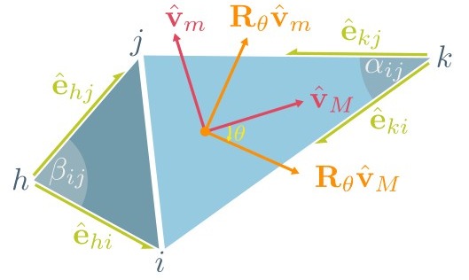
The inner products between the edge versors are weighted by a shear matrix . is the matrix containing a local reference frame defined on a face, with being the normal to the surface and , being the orthogonal components defined on the face — a common choice involves using the principal curvatures and setting and . is the rotation matrix rotating the reference frame, and is a diagonal matrix controlling the anisotropy. When we have , thus and . This reduces Eq. (1) to the traditional isotropic LBO formulation, which we indicate with . For we have the anisotropic LBO (ALBO), which we indicate as .
边单位向量之间的内积由剪切矩阵 加权。 是定义在一个面上的局部参考系矩阵,其中 是表面法向,、 是面上的正交分量——常见做法是采用主曲率方向,并取 、。 是旋转该参考系的旋转矩阵, 是控制各向异性的 对角矩阵。当 时,,于是 ,且 。这时式 (1) 就退化成传统的各向同性 LBO,我们把它记为 。当 时,得到各向异性 LBO(ALBO),记为 。
The generalised eigendecomposition of the LBO can be written as , where represents the first eigenvectors defined at the vertices of the mesh, and is the diagonal matrix containing the eigenvalues. The eigendecomposition of the ALBO follows the same procedure to determine the - and -dependent and .
LBO 的广义特征分解可写成 ,其中 表示定义在网格顶点上的前 个特征向量, 是由特征值构成的对角矩阵。ALBO 的特征分解沿用同一手续,以得到依赖于 和 的 与 。
Heat Diffusion and Kernels. The heat diffusion process over a mesh is mathematically described as: , where the vertex-valued scalar function represents how an initial heat distribution over evolves for times . Indicating with the vector obtained by evaluating for all vertices, the solution of the heat equation has the form [9,12,34,37]:
热扩散与热核。 网格上的热扩散过程可写成 ,其中定义在顶点上的标量函数 描述 上的初始热量分布如何随时间 演化。用 表示在所有顶点上计算 得到的向量,则热方程的解具有如下形式 [9,12,34,37]:
When the initial distribution is a delta function, , Eq. (2) is referred to as heat kernel and it represents how the heat generated by a single point source diffuses over the surface. In Euclidean space, it has the explicit expression of a Gaussian [36]. Note that while it is possible to simulate the diffusion by solving a sparse linear system, the spectral approach we adopt proved to be one order of magnitude faster and to scale to high-resolution meshes [34].
当初始分布是一个 delta 函数,即 时,式 (2) 被称为热核,它描述单个点源产生的热量如何在表面上扩散。在欧氏空间中,它具有高斯的显式表达式 [36]。需要说明的是,虽然也可以通过求解稀疏线性系统来模拟扩散,但我们采用的谱方法已被证明大约快一个数量级,并且能够扩展到高分辨率网格 [34]。
4 Heat Kernel Textures
4 热核纹理
We now detail our HKTex model, which uses arbitrarily positioned heat kernels to intrinsically represent textures directly on the surface of manifold meshes.
下面详细介绍我们的 HKTex 模型:它使用可任意放置的热核,在流形网格表面上内蕴地表示纹理。
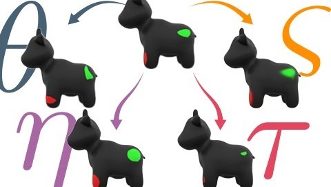
Kernel parameters. We define our HKTex as a collection of optimisable heat kernels, . Each kernel is parametrised as , where is the position of the heat source, and are the angle and anisotropy controlling the diffusion process, is the threshold controlling the scale of the kernel, is the parameter controlling the sharpness of its border, and is the RGB colour. The parameters of all are jointly optimised.
核参数。 我们把 HKTex 定义成 个可优化热核的集合 。每个核参数化为 ,其中 是热源位置, 与 是控制扩散过程的角度与各向异性, 是控制核尺度的阈值, 控制其边界锐度, 是 RGB 颜色。集合 中全部核的参数一起联合优化。
Normalised heat kernels. In Sec. 3 we have introduced the discrete formulation of heat kernels and diffusion. While this is the gold standard on 3D meshes, we seek to break free from the mesh discretisation and represent textures beyond vertices. We thus leverage the continuous manifold formulation of heat kernels and define how to transform discrete quantities into continuous ones. Anisotropically heat diffusing a Dirac delta function centred in for a time , we have the truncated continuous anisotropic heat kernel:
归一化热核。 第 3 节已经给出热核与扩散的离散表述。这在三维网格上虽是金标准,但我们希望摆脱网格离散化的束缚,把纹理表示扩展到顶点以外。因此我们借助热核的连续流形表述,并说明如何把离散量变成连续量。将以 为中心的 Dirac delta 函数做时间为 的各向异性热扩散,便得到截断的连续各向异性热核:
where is any arbitrary point on the surface of , is the -th eigenvalue with its corresponding eigenfunction evaluated at or , and is the mass at the source. Since the physical heat diffusion process conserves energy, as heat spreads, the source temperature decreases. Therefore, the size and shape of kernels would affect their overall temperature. To stabilise optimisation and make filtering predictable, we guarantee a maximum temperature of at the kernel centre by normalising with respect to the post-diffusion source temperature:
其中 是 表面上的任意点, 是第 个特征值,对应的特征函数 在 或 处求值, 是源点处的质量。物理上的热扩散过程守恒能量,热量扩散开后,源点温度会下降。因此,核的大小和形状会影响其整体温度。为了稳定优化并使过滤可预期,我们按扩散后源点温度做归一化,保证核中心的最高温度为 :
Biharmonic distance weighting. Heat kernels have a global support across the entire surface of the object. While they should decay with distance from the heat source, since we adopt a spectral truncation to the most significant frequencies, the kernels suffer from a Gibbs-like phenomenon [30,31] producing spectral ringing artifacts in distant regions (see supplementary materials). To suppress these unwanted artifacts and enforce local support, we introduce a Biharmonic distance Gaussian weighting that dampens the contributions of distant kernels. We compute the Biharmonic distance [20] using isotropic eigenproperties: . Then, we weight our normalised kernels:
双调和距离加权。 热核在整个物体表面上具有全局支集。按理说它应随离开热源的距离衰减,但由于我们采用谱截断、只保留 个最显著频率,这些核会出现类似 Gibbs 的现象 [30,31],在远处区域产生频谱振铃伪影(见补充材料)。为抑制这些不需要的伪影并强制局部支集,我们引入双调和距离上的高斯加权,以减弱远处核的贡献。双调和距离 [20] 用各向同性的特征量计算:。然后,我们这样加权归一化后的核:
Kernel filtering. produces a Gaussian-like geodesic kernel, with values in , that gradually fades from the source location. Instead of optimising the diffusion time to scale the kernel, we fix and modulate kernel scale () and sharpness () via a rescaled soft-step filtering function:
核过滤。 会得到一个类似高斯的测地核,取值在 ,并从源位置逐渐减弱。我们不通过优化扩散时间来缩放核,而是固定 ,再用经过重标定的软阶跃过滤函数来调节核的尺度()与锐度():
where is a sigmoid function. This filtering preserves the value range and provides more control over the kernel appearance, which can now be easily scaled down to point-sized dimensions while controlling the rate of signal decay. A filtered kernel can now either preserve its characteristic fading appearance or transform into a crisp geodesic ellipsoid defined on the surface of the mesh.
其中 是 sigmoid 函数。这种过滤保持 的取值范围,并对核的外观提供更多控制:现在可以方便地把核缩小到接近点的尺度,同时控制信号衰减的速度。过滤后的核既可以保留其特有的渐隐外观,也可以变成定义在网格表面上的清晰测地椭球。
Colour formation. For a given kernel , we denote its evaluated spatial footprint as . To determine the final texture colour at a surface point , we need to aggregate the contributions of all kernels. Inspired by [49], we select the top-contributing kernels to . In our formulation, this can be achieved by dynamically identifying the kernels with the highest . The local texture is then computed via an alpha-weighted partition of unity over these selected kernels (), which is added as a residual to an optimisable global base colour :
颜色形成。 对给定核 ,我们把它求值后的空间足迹记为 。要确定表面点 处的最终纹理颜色 ,需要聚合所有核的贡献。受 [49] 启发,我们选出对 贡献最大的 个核。在我们的表述中,这可以通过动态找出 最高的那些核来完成。局部纹理随即在这些被选中的核()上,按 alpha 加权的单位分解计算,并作为残差加到可优化的全局底色 上:
This colour formation paradigm guarantees a controlled blending between locally overlapping kernels, while empty regions seamlessly default to the underlying base colour.
这一颜色形成方式保证了局部重叠的核之间能够受控地混合,而空白区域则会自然回退到底层底色。
4.1 Parametric Interpolation of the Spectral Bases
4.1 谱基底的参数插值
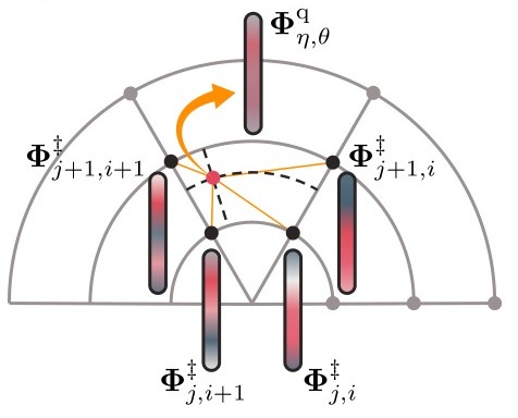
Interpolation of ALBO eigenproperties. Evaluating the continuous anisotropic heat kernel in Eq. (3) requires the spectral properties associated with a kernel's specific shape parameters . Since constructing and eigendecomposing a unique ALBO for every kernel during an optimisation pipeline is computationally prohibitive, we devise a simplified and easily differentiable alternative. We thus discretise the parameter space of angles and anisotropies into a half-polar-like grid, where anisotropies are log-scaled to make the space more perceptually uniform and prevent high anisotropies from dominating. We associate each grid node , located at discrete angle and log-scaled anisotropy , with its precomputed and . To evaluate a continuous kernel query with parameters , we first project the queried anisotropy into the same logarithmic space, . We then perform a binary search to identify the bounding grid cell indices and such that and . Within this cell, we compute the normalized local coordinates: and . The queried eigenproperties are then efficiently approximated via bilinear interpolation over the four cell corners :
ALBO 特征量的插值。 计算式 (3) 中的连续各向异性热核,需要与该核特定形状参数 相对应的谱性质。如果在优化过程中为每个核都构造并特征分解一套独特的 ALBO,计算上难以承受,因此我们设计了一种更简化、也易于微分的替代方案。于是我们把角度与各向异性的参数空间离散成一个半极坐标式的网格,其中各向异性做对数缩放,以使该空间在感知上更均匀,并避免高各向异性占主导。我们为每个位于离散角度 与对数各向异性 处的网格节点 ,预先计算 与 。要计算参数为 的连续核查询,先把查询的各向异性投影到同一对数空间,。再通过二分搜索确定包围该查询的网格单元指标 、,使得 且 。在该单元内计算归一化局部坐标:,。随后,在该单元四个角点 上做双线性插值,即可高效近似所查询的特征量:
where the interpolation weights are derived from the fractional distances and (i.e., , , etc.).
其中插值权重 由分数距离 与 得到(例如 ,,以此类推)。
Alignment of precomputed ALBO eigenproperties. When eigendecomposing the precomputed ALBOs, we observe the same permutation, rotations, and sign ambiguities that are widely observed in shape matching problems (e.g., [27]). Since this behaviour would hinder the correctness of the bilinear interpolation in Eq. (8), we introduce an eigenproperties alignment procedure during the grid construction and thus ensure that all and are consistent with the and of the isotropic LBO. First, we resolve the permutation switching issue by maximizing the mass-weighted cross-correlation between two sets of eigenvectors: and . We compute the correlation matrix and apply the Hungarian algorithm to find the optimal assignment matrix , yielding the permuted eigenvectors . Next, we solve the Orthogonal Procrustes problem minimising the mass-weighted Frobenius distance via the Singular Value Decomposition (SVD) of . The resulting rotation determines . Finally, we correct the sign flips by constructing a diagonal matrix where . The fully aligned spectral basis stored at each grid node is thus obtained as . Eigenvalues are simply reordered according to . The initial reference eigenvectors are those of the LBO, then we use the last set aligned during the grid construction. Hereafter, we consider all and to be implicitly aligned for ease of notation.
预计算 ALBO 特征量的对齐。 在对预计算的 ALBO 做特征分解时,我们观察到与形状匹配问题中常见的同样排列、旋转和符号歧义(例如 [27])。这种行为会破坏式 (8) 中双线性插值的正确性,因此我们在构建网格时引入特征量对齐步骤,从而保证所有 与 都与各向同性 LBO 的 、 相一致。首先,通过最大化两组特征向量 与 之间按质量加权的互相关,来解决排列交换问题。我们计算相关矩阵 ,并用匈牙利算法求最优分配矩阵 ,得到排列后的特征向量 。接着,我们求解正交 Procrustes 问题,通过 的奇异值分解(SVD),最小化按质量加权的 Frobenius 距离 。由此得到的旋转给出 。最后,构造对角矩阵 ,其中 ,以校正符号翻转。于是,存储在每个网格节点上、完全对齐后的谱基底为 。特征值只需按 重新排序。最初的参考特征向量取自 LBO,随后使用网格构建过程中最近一次对齐得到的那一组。此后为书写简便,我们默认所有 与 都已隐式对齐。
4.2 Spatial Evaluation of Spectral Properties and Masses
4.2 谱性质与质量的空间求值
Continuous spatial evaluation. All precomputed spectral properties are strictly defined on the vertices of . Limiting kernel placement and evaluation exclusively to these locations would bind our model to the surface discretisation. To overcome this limitation and evaluate any vertex-based spectral quantity at an arbitrary continuous location , we exploit the inherent smoothness of the spectral bases. Inspired by [12], we approximate this continuous spatial evaluation via barycentric interpolation: .
连续空间求值。 所有预计算的谱性质都严格定义在 的顶点上。如果把核的放置和求值都限制在这些位置,模型就会被绑在表面的离散化上。为克服这一限制,并在任意连续位置 上计算任何定义在顶点上的谱量 ,我们利用谱基底固有的光滑性。受 [12] 启发,我们用重心插值来近似这种连续空间求值:。
Biharmonic KNN search. Evaluating the heat equation for all kernels and target points using Eq. (3), yields an intractable complexity. Because our biharmonic distance weighting (Eq. (5)) forces kernels to decay to zero outside a local radius, we can safely prune distant sources. We define a spectral embedding at the vertices as . In this space, Euclidean distance corresponds to the biharmonic distance on the manifold. Using our continuous evaluation strategy, we compute these embeddings for kernel sources and target points as and . We then construct a K-Nearest Neighbours (KNN) graph in this embedded space to dynamically restrict the evaluation of each point to only its nearest sources .
双调和 KNN 搜索。 若用式 (3) 对全部 个核和 个目标点计算热方程,复杂度将达到难以承受的 。由于双调和距离加权(式 (5))会迫使核在局部半径之外衰减到零,我们可以安全地剪掉远处的源。我们在顶点上定义谱嵌入 。在这一空间中,欧氏距离对应于流形上的双调和距离 。利用前面的连续求值策略,核源与目标点的嵌入可写成 以及 。随后在该嵌入空间中构建 近邻(KNN)图,从而把每个点 的求值动态限制在其 个最近源 上。
Local anisotropic evaluation. Once the local subset of sources is identified, we must evaluate the continuous anisotropic eigenfunctions specifically required by those sources. Rather than computing the basis for all kernels globally, we retrieve the queried discrete eigenvectors corresponding to the specific shape parameters of only the neighbouring sources. Applying our continuous evaluation strategy, we approximate these source-specific eigenfunctions at both the source location and the target location . Specifically, we compute and . This dual evaluation allows us to construct the heat kernel between and (Eq. (3)), while keeping the computational complexity strictly bounded to .
局部各向异性求值。 一旦确定了局部源子集 ,就必须计算这些源所特别需要的连续各向异性特征函数。我们并不为所有核全局计算基底,而是只取这 个邻近源在其特定形状参数 下查询得到的离散特征向量 。再利用连续求值策略,在源位置 和目标位置 上近似这些源特有的特征函数。具体而言,我们计算 以及 。这种双向求值使我们能构造 与 之间的热核(式 (3)),同时把计算复杂度严格限制在 。
Mass definition for arbitrary points on . Finally, evaluating the continuous heat kernel (Eq. (3)) requires the mass at the continuous source point . Since the discrete mass matrix () is proportional to vertex areas and thus local sampling density, we cannot simply use barycentric interpolations like we did for the eigenvectors. We thus formulate a Kernel Density Estimation (KDE) approach to correctly estimate the mass of every point based on the density of surrounding points (see supplementary materials). While this approach approximates the real mass, we empirically find that assigning a uniform unit mass to all sources () is significantly faster and does not deteriorate performance. Because the pointwise evaluation depends solely on the source mass as a linear scalar (Eq. (3)), during optimisation the other kernel properties can learn to compensate for the missing local integration weights.
上任意点的质量定义。 最后,计算连续热核(式 (3))还需要连续源点 处的质量 。由于离散质量矩阵()与顶点面积成正比,因而也与局部采样密度成正比,我们不能像对待特征向量那样直接做重心插值。于是我们构造了一种核密度估计(KDE)方法,根据周围点的密度来正确估计每个点的质量(见补充材料)。这一方法只是在近似真实质量;我们在实验中发现,给所有源赋均匀的单位质量()要快得多,而且不会损害性能。因为逐点求值只通过一个线性标量依赖源质量(式 (3)),优化过程中其他核属性可以学会补偿所缺失的局部积分权重。
4.3 Optimisation & Density Control
4.3 优化与密度控制
Geodesic position optimisation. Standard Euclidean optimisation would apply gradient updates directly to the 3D coordinates, inevitably pulling the heat kernel sources off the mesh surface. Since sources are intrinsically defined on , we must restrict movements exclusively to the surface. We thus formulate a Riemannian gradient descent optimiser: each gradient is projected to the local tangent plane and scaled to define an initial velocity . We then compute the exponential map , tracing the geodesic defined by this vector to determine the updated kernel position. To accelerate convergence with momentum, we parallel transport the accumulated momentum to the new kernel position. Both the exponential map and parallel transport are computed via the straightest geodesic algorithm [32], utilising the optimisation-friendly and CUDA-parallelised implementation introduced by [38].
测地位置优化。 标准的欧氏优化会把梯度更新直接加在三维坐标上,不可避免地把热核源拉离网格表面。由于源 是内蕴地定义在 上的,移动必须被限制在表面上。因此我们构造黎曼梯度下降优化器:每个梯度 被投影到局部切平面 上,再缩放得到初始速度 。随后计算指数映射 ,沿该向量所定义的测地线追踪,以确定更新后的核位置。为用动量加快收敛,我们把累积动量平行移动到新的核位置。指数映射与平行移动都通过最直测地线算法 [32] 计算,并采用 [38] 提出的便于优化、且经 CUDA 并行化的实现。
Kernel pruning strategy. Like most Gaussian Splatting techniques, we adaptively control the density of our heat kernels throughout the optimisation process. In order to decrease computational overhead and storage costs, we aim to delete kernels that contribute little to the final texture. During an accumulation window , we record two metrics for every kernel : a hit count indicating how frequently it is selected in the local partition of unity (Eq. (7)), and an energy score aggregating its filtered weights . Periodically, we prune kernels that are either rarely hit () or energetically weak ().
核剪枝策略。 与大多数高斯溅射技术类似,我们在整个优化过程中自适应地控制热核密度。为降低计算开销和存储成本,我们希望删掉对最终纹理贡献很少的核。在累积窗口 内,我们为每个核 记录两项指标:命中次数 ,表示它在局部单位分解 (式 (7))中被选中的频率;以及能量分数 ,汇总其过滤后的权重 。我们定期剪掉很少被命中的核(),或能量过弱的核()。
Kernel densification strategy. To capture missing details, we dynamically densify kernels based on local reconstruction error. Over an accumulation window , we compute the spatial error and distribute it to contributing kernels weighted by their normalised partition of unity, yielding a per-kernel score . Kernels exceeding an error threshold are densified according to their spatial extent (). Small kernels () are cloned in place, allowing the optimiser to naturally separate them. Large kernels () are split into two smaller kernels. Crucially, to respect manifold constraints during splitting, we displace the new kernels along their principal axis using the exponential map provided by [38]. A maximum growth ratio caps additions per step to ensure stability.
核加密策略。 为补上缺失的细节,我们根据局部重建误差动态加密核。在累积窗口 内,计算空间误差 ,再按归一化后的单位分解权重把它分配给各个贡献核,得到每个核的分数 。超过误差阈值 的核,按其空间范围()进行加密。小核()就地克隆,让优化器自然地把它们分开。大核()则被分裂成两个更小的核。关键在于,为在分裂时尊重流形约束,我们借助 [38] 提供的指数映射,沿主轴移动新核。每一步的新增数量由最大增长比 封顶,以保证稳定。
4.4 Rendering & Applications
4.4 渲染与应用
Physically based rendering. Because our HKTex formulation is continuously evaluated across , it seamlessly integrates into modern physically based rendering (PBR) pipelines. We implement HKTex also as a differentiable texture within the Mitsuba3 renderer [16]. During ray tracing, when a ray intersects the mesh at an arbitrary continuous point , the renderer queries the corresponding local subset of kernels and computes following Eq. (7). By wrapping our PyTorch-based evaluation within Dr.Jit [15], we allow gradients to backpropagate directly from the rendered image pixels to our intrinsic kernel parameters.
基于物理的渲染。 由于 HKTex 的表述在整个 上连续求值,它可以无缝接入现代的基于物理的渲染(PBR)流水线。我们还把 HKTex 实现为 Mitsuba3 渲染器 [16] 中的可微纹理。光线追踪时,当光线在任意连续点 处与网格相交,渲染器会查询对应的局部核子集 ,并按式 (7) 计算 。通过把基于 PyTorch 的求值封装进 Dr.Jit [15],我们可以让梯度从渲染得到的图像像素直接回传到内蕴的核参数。
Optimise existing UV-textures. When a ground-truth UV texture is available, we can directly optimise our kernels. At each optimisation step, we uniformly sample a dense set of points directly on the faces of , and evaluate their colour with . Our HKTex model is then updated by minimizing the photometric error with respect to , the colour queried from the UV texture at the same location: .
优化已有 UV 纹理。 当有真值 UV 纹理可用时,我们可以直接优化这些核。在每一步优化中,我们在 的面上均匀采样一组密集的点 ,并用 计算它们的颜色。随后通过最小化相对于 ——即同一位置从 UV 纹理查询到的颜色——的光度误差来更新 HKTex 模型:。
Optimise multi-view images. Our HKTex model can also be optimised from multi-view images via the differentiable PBR renderer. In this scenario, we suppose the target mesh to be given alongside a set of camera poses. At each training step, we sample camera views, identify all the rays hitting the mesh across views, and select a random subset to provide uniform coverage around the object. Minimising the rendering error against the ground-truth pixels at the ray intersections drives the HKTex optimisation.
优化多视图图像。 HKTex 也可以通过可微的 PBR 渲染器,从多视图图像进行优化。在这一设定中,我们假定目标网格与一组相机位姿一并给出。每一步训练时,我们采样 个相机视角,找出各视角中所有打到网格上的光线,再随机选取一个子集,以在物体周围提供均匀覆盖。最小化光线交点处相对于真值像素的渲染误差,就推动了 HKTex 的优化。
5 Experiments
5 实验
5.1 Data
5.1 数据
We conduct experiments on a curated subset of Objaverse [11]. Since the full dataset comprises scraped online assets, mesh quality is not guaranteed. We therefore filter for objects that possess LVIS category labels, valid textures, and at least one community like and view, while excluding point clouds and animated models. To maintain a reasonable computational overhead, we restrict the maximum vertex count to . To ensure compatibility with our HKTex representation, we also define a rigorous geometric filtering: we exclude meshes with multiple disconnected components, with non-manifold geometries, and with complex internal structures (i.e. models presenting more than 20 intersections on any ray cast from a regular grid defined on the bounding box of the object). Finally, since our method is heavily reliant on the eigenfunctions of LBO, we reject models where such eigendecomposition fails. After filtering, we retain high-quality models. Note that while having an eigendecomposable LBO is essential, our filtering criteria can be relaxed at the cost of overall dataset quality or of separately processing parts of non-manifold and complex meshes. When fitting multi-view images, meshes are rendered with their albedos as the sole texture map.
我们在经过筛选的 Objaverse [11] 子集上开展实验。由于完整数据集由网上抓取的资产组成,网格质量并无保证。因此我们筛选出带有 LVIS 类别标签、有效纹理,并且至少有一次社区点赞和浏览的物体,同时排除点云和动画模型。为把计算开销控制在合理范围,我们将最大顶点数限制为 。为与 HKTex 表示相容,我们还设定了严格的几何过滤:排除具有多个不连通部件、非流形几何,以及内部结构过于复杂的网格(即从物体包围盒上规则网格射出的任意射线上,相交次数超过 20 的模型)。最后,由于方法高度依赖 LBO 的特征函数,特征分解失败的模型也被剔除。过滤之后,我们保留约 个高质量模型。需要说明的是,虽然 LBO 必须能够做特征分解,但这些过滤条件可以放宽,代价是整体数据质量下降,或需要把非流形和复杂网格的部件分开处理。在拟合多视图图像时,网格仅用其反照率作为纹理贴图来渲染。
5.2 Implementation details
5.2 实现细节
Our HKTex pipeline is built with PyTorch [29], utilizing the GPU version of FAISS [17] for the biharmonic distance KNN search and Mitsuba3 [16] with Dr.Jit [15] for differentiable ray tracing. Instead of building specialized CUDA kernels, we use PyTorch's Triton code generation [3]. For all meshes, we precompute a 64-dimensional eigendecomposition of the isotropic LBO for calculating biharmonic distances, and 256-dimensional eigendecompositions for all the ALBOs in our grid with the cross product of 7 angles and 7 anisotropies. The network parameters are initialized as in the following paragraph, and we use a projected gradient descent (PGD) algorithm to enforce the correct ranges. For all parameters except kernel locations, we use an Adam optimiser with a step-function learning rate scheduler for fitting UV-textures and multi-view images. To optimize kernel locations, we utilize a geodesic Riemannian-SGD algorithm on the GPU using the library from [38]. We run a short Bayesian hyperparameter tuning on 5 meshes excluded from the evaluation dataset for both setups using Optuna [1] with the Tree-Structured Parzen Estimator [4], and we share the exact hyperparameters in our supplementary. We use an importance sampling strategy, as detailed in our supplementary material, when fitting UV-textures. To render our output images and to perform differentiable ray tracing for inverse rendering, we utilize Mitsuba3 [16] with Dr.Jit [15]. We use a path-replay backpropagation (PRB) integrator with a ray depth of 3 for training, and differentiate through the ray tracing process to optimize our textures. During inference, we only build the KNN database and pre-compute the self-reference heat kernels once, reducing computation significantly. We use the tuned hyperparameters to set the pruning and densification hyperparameters for both settings.
HKTex 流水线用 PyTorch [29] 搭建,双调和距离上的 KNN 搜索使用 FAISS [17] 的 GPU 版本,可微光线追踪则使用带 Dr.Jit [15] 的 Mitsuba3 [16]。我们没有编写专门的 CUDA 核,而是使用 PyTorch 的 Triton 代码生成 [3]。对所有网格,我们预先计算 64 维的各向同性 LBO 特征分解以用于双调和距离,并在由 7 个角度与 7 个各向异性叉乘得到的网格上,为所有 ALBO 预计算 256 维特征分解。网络参数按下一小节初始化,并用投影梯度下降(PGD)算法把参数限制在正确范围内。除核位置外的所有参数,在拟合 UV 纹理和多视图图像时都使用带阶梯学习率调度的 Adam 优化器。核位置则使用 [38] 提供的程序库,在 GPU 上用测地黎曼 SGD 算法优化。我们在两个设定下,都用 Optuna [1] 和 Tree-Structured Parzen Estimator [4],在 5 个排除在评估集之外的网格上做了简短的贝叶斯超参数调节,并在补充材料中给出了确切的超参数。拟合 UV 纹理时,我们采用补充材料中详述的重要性采样策略。输出图像的渲染,以及反渲染中的可微光线追踪,都使用带 Dr.Jit [15] 的 Mitsuba3 [16]。训练时采用路径回放反向传播(PRB)积分器,光线深度为 3,并穿过光线追踪过程求微分以优化纹理。推理时只需构建一次 KNN 数据库并预计算自参照热核,从而显著减少计算。两个设定下的剪枝与加密超参数,都使用调好的超参数来设置。
Initialisation. We use a uniform sampling strategy based on mesh area to first oversample a large number of points on the mesh surface, and then use farthest-point sampling to obtain kernel locations and face indices. The kernel colours are sampled from a uniform distribution between -1 and 1, with the mean subtracted and the mean set to our global base colour. The angles and anisotropies are sampled from a uniform distribution between 0 and and 1 and 100, respectively. For sharpness and threshold initialization, we sample from the beta distributions and , respectively. Then, the sharpnesses are scaled and shifted to the range 10–50, and the thresholds to 0.9–1.0 (0.7–1.0 for the multi-view rendering case). The parameters are then optimized, as detailed before and in the supplementary, using PGD.
初始化。 我们先按网格面积做均匀采样,在网格表面上过采样大量点,再用最远点采样得到核位置和面索引。核颜色从 到 的均匀分布中采样,减去均值后再把均值设为全局底色。角度从 到 的均匀分布中采样,各向异性从 到 的均匀分布中采样。锐度和阈值的初始化分别从 beta 分布 与 中采样。随后把锐度缩放并平移到 –,阈值平移到 –(多视图渲染时为 –)。这些参数再按前文及补充材料所述,用 PGD 进行优化。
5.3 Evaluation metrics
5.3 评价指标
To quantitatively assess textures against the ground truth, we render five distinct views for each object and measure image metrics on them. In particular, we compute Mean Squared Errors (MSE) and Peak Signal-to-Noise Ratio (PSNR). To evaluate the preservation of structural details and contrast, we use the Structural Similarity Index (SSIM) and its multi-scale variant (MS-SSIM). Furthermore, we report the Learned Perceptual Image Patch Similarity (LPIPS) to measure perceptual quality. Finally, to validate our core claim of memory efficiency, we report the total Storage footprint in kilobytes (KB), strictly accounting for all intrinsic parameters, network weights, and any topological overheads (e.g., UV-coordinates) required by the baselines. We store with the same formats and without method-specific quantizations. Identical zip compression was already applied across all methods to provide a fair baseline for comparing intrinsic information density.
为定量评估纹理相对真值的表现,我们为每个物体渲染五个不同视角,并在这些图像上计算指标。具体包括均方误差(MSE)和峰值信噪比(PSNR)。为评估结构细节与对比度的保持情况,我们使用结构相似性指数(SSIM)及其多尺度变体(MS-SSIM)。此外还报告学习感知图像块相似度(LPIPS),以衡量感知质量。最后,为验证我们关于内存效率的核心主张,我们报告以千字节(KB)计的总存储占用,严格计入全部内蕴参数、网络权重,以及基线方法所需的任何拓扑开销(例如 UV 坐标)。各方法采用相同的存储格式,并且不做方法特有的量化。所有方法都已施加相同的 zip 压缩,以便公平比较内蕴信息密度。
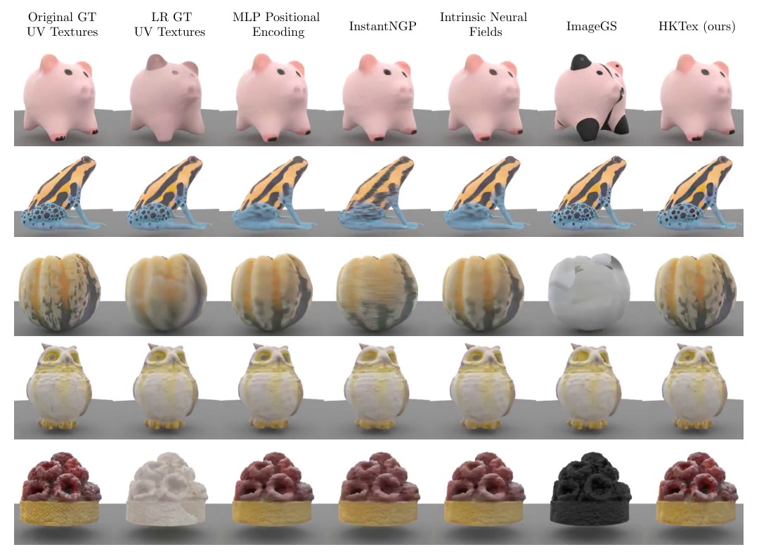
Fig. 2: Qualitative comparison against SotA methods. With the exception of the GT UV Textures, all other methods have similar or bigger storage size. For visual clarity, we render only the albedo textures under constant ambient illumination.
图 2:与当前最先进方法的定性比较。除真值 UV 纹理外,其余方法的存储占用相当或更大。为便于观察,我们只在恒定环境光照下渲染反照率纹理。
5.4 Fitting UV-textures
5.4 拟合 UV 纹理
We first demonstrate our method's ability to represent existing UV textures at a significantly reduced storage cost. We optimise our HKTex against the ground truth albedo UV-texture of 313 meshes, arbitrarily selected from our curated dataset. We then quantitatively and qualitatively compare against leading state-of-the-art intrinsic texture representations and image-based baselines under strictly matched memory budgets.
我们首先展示,该方法能以显著更低的存储成本表示已有的 UV 纹理。在从筛选数据集中任意选取的 313 个网格上,我们用真值反照率 UV 纹理优化 HKTex。随后在严格对齐的内存预算下,与领先的内蕴纹理表示以及基于图像的基线做定量和定性比较。
For the neural baselines, we implement three multilayer perceptrons (MLPs) taking as input different positional encodings of the ray-intersection points. Specifically, we evaluate a standard MLP with traditional Fourier positional encoding [23], an adaptation of InstantNGP [24] utilizing hash-grid encoding, and Intrinsic Neural Fields [19], which barycentrically interpolates the eigenvectors of the LBO. To ensure a fair comparison, we conduct a grid search over the network width, depth, and hash-grid size to exactly match the storage cost of our optimised HKTex.
神经基线方面,我们实现了三个多层感知机(MLP),输入为光线交点上不同的位置编码。具体而言,我们评估了使用传统傅里叶位置编码的标准 MLP [23]、采用哈希网格编码的 InstantNGP 改写版本 [24],以及通过对 LBO 特征向量做重心插值的 Intrinsic Neural Fields [19]。为保证公平比较,我们对网络宽度、深度和哈希网格大小做网格搜索,以精确匹配优化后 HKTex 的存储成本。
Furthermore, we compare against two explicit 2D baselines: downsampled ground-truth images and ImageGS [49] (a 2D Gaussian Splatting approach). Crucially, both image-based methods fundamentally rely on UV-mapping. Even when the UVmap is provided, the storage of per-vertex UV-coordinates incurs a fixed memory overhead that must be accounted for in the total texture budget. Consequently, for meshes with high vertex counts, this overhead dominates the budget, severely restricting the memory available for the actual texture or 2D Gaussians. As shown in Tab. 1, an exact storage match is often impossible for these baselines; even when limiting the downsampled texture to a minimum resolution of pixels and ImageGS to just 10 Gaussians, the performance penalty is catastrophic for densely sampled meshes (Fig. 2).
此外,我们还与两种显式二维基线比较:降采样后的真值图像,以及 ImageGS [49](一种二维高斯溅射方法)。关键在于,这两种基于图像的方法根本上都依赖 UV 映射。即便提供了 UV 图,逐顶点 UV 坐标的存储仍会带来固定的内存开销,必须计入总的纹理预算。因此,对于顶点很多的网格,这项开销会占满预算,严重限制真正可用于纹理或二维高斯的内存。如表 1 所示,这些基线往往无法做到存储完全对齐;即便把降采样纹理限制到最低 像素、把 ImageGS 限制到仅 10 个高斯,在稠密采样的网格上性能损失也是灾难性的(图 2)。
Finally, we compare against vertex colours directly sampled from the GT UV-textures at the native mesh resolution (GT VTex) as well as iteratively subdividing the mesh to match our storage budget (HR GT VTex).
最后,我们还与直接从真值 UV 纹理、按网格原生分辨率采样的顶点颜色(GT VTex)进行比较,以及为匹配我们的存储预算而迭代细分网格后的顶点颜色(HR GT VTex)。
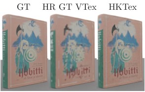
Fig. 3: Comparison with vertex colours.
图 3:与顶点颜色的比较。
As reported in Tab. 1, HKTex achieves the lowest storage footprint after GT VTex while maintaining competitive reconstruction quality across all metrics. Although LR GT UV-textures achieve the highest PSNR due to directly storing image samples, our representation yields the second best perceptual quality (LPIPS) and the best SSIM, MS-SSIM, and MSE, indicating improved preservation of structural details despite using fewer parameters. Neural baselines and HR GT VTex require significantly larger storage budgets to achieve almost comparable accuracy, highlighting the efficiency of our geodesic heat kernel representations.
如表 1 所示,HKTex 的存储占用仅高于 GT VTex,同时在全部指标上保持有竞争力的重建质量。低分辨率真值 UV 纹理因直接存储图像样本而取得最高的 PSNR,但我们的表示得到了第二好的感知质量(LPIPS),以及最好的 SSIM、MS-SSIM 和 MSE,说明尽管参数更少,对结构细节的保持反而更好。神经基线与高分辨率顶点颜色(HR GT VTex)需要显著更大的存储预算,才能达到几乎相当的精度,这凸显了测地热核表示的效率。
The qualitative comparisons in Fig. 2 further highlight the behaviour of the different representations. Neural field baselines tend to oversmooth fine texture details, particularly in regions with sharp colour transitions or high-frequency patterns (e.g., the frog and raspberry examples). ImageGS occasionally produces noticeable artifacts due to the limited number of splats available under the storage constraints, sometimes failing to capture the correct colour distribution. Vertex colours, even when subdivided (Fig. 3), fail to correctly represent textures because the vertex positioning is determined by geometry rather than texture content. In contrast, HKTex preserves sharper texture boundaries and more faithful colour distributions across objects while remaining within the same or smaller storage budgets.
图 2 中的定性比较进一步凸显了不同表示的行为。神经场基线往往把细腻的纹理细节抹得过平,尤其是在颜色过渡陡峭或高频图案的区域(例如青蛙和覆盆子这两个例子)。ImageGS 有时会因为存储约束下可用的溅射数量有限而产生明显伪影,偶尔无法捕捉正确的颜色分布。顶点颜色即便经过细分(图 3),也难以正确表示纹理,因为顶点位置由几何而不是纹理内容决定。相比之下,HKTex 能在相同或更小的存储预算内,在不同物体上保持更锐利的纹理边界和更忠实的颜色分布。
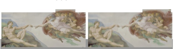
Fig. 4: Image on two triangles.
图 4:画在两个三角形上的图像。
Fitting Images. To test HKTex's ability to represent high-resolution textures on coarse meshes, we fit an image onto a rectangle made of two triangles. In this special case of UV-texture fitting, we found it beneficial to amplify the weighted and normalised kernels as before filtering them (with ). Nevertheless, is sufficient for most meshes.
拟合图像。 为检验 HKTex 在粗糙网格上表示高分辨率纹理的能力,我们把一幅图像拟合到由两个三角形构成的矩形上。在这一特殊的 UV 纹理拟合情形中,我们发现在过滤前把加权并归一化的核放大为 (取 )是有益的。不过,对大多数网格而言, 就足够了。
5.5 Fitting multi-view images
5.5 拟合多视图图像
To demonstrate our method's ability to optimize multi-view images, we create a synthetic training scenario in which, instead of UV textures, we use rendered images of the ground-truth UV textures, following the same data setup in UV texture fitting but with a smaller subset of the data. To generate training data, we sample rays from random views during training and select a random subset to form minibatches at each epoch.
为展示该方法优化多视图图像的能力,我们构造了一个合成训练场景:不再使用 UV 纹理,而是使用真值 UV 纹理渲染出的图像;数据设置与 UV 纹理拟合相同,但子集更小。为生成训练数据,我们在训练过程中从随机视角采样光线,并在每个 epoch 随机选取一个子集组成小批量。
Similar to the UV fitting setup, we implement two MLP architectures conditioned on different positional encodings, corresponding to the spatially varying albedo map. For a fair comparison, these representations are also trained using automatic differentiation and the interoperability between Mitsuba3 and PyTorch. The first baseline utilizes traditional positional encodings. The second baseline is an adaptation of NVDiffRec [25], with the mesh and environment map fixed to the ground-truth mesh and environment map using hash encoding and with only the albedo map output. Like in the uv-fitting setting, we also conduct a grid search over the width, depth, and the hash-grid size to try to match the storage cost of our model.
与 UV 拟合设定类似,我们实现了两个由不同位置编码条件化的 MLP 架构,对应于空间变化的反照率图。为公平比较,这些表示同样借助 Mitsuba3 与 PyTorch 的互操作,用自动微分训练。第一条基线使用传统位置编码。第二条基线是 NVDiffRec [25] 的改写版本:网格与环境贴图被固定为真值网格与环境贴图,采用哈希编码,并且只输出反照率图。与 uv 拟合设定一样,我们也对宽度、深度和哈希网格大小做网格搜索,以尽量匹配我们模型的存储成本。
As shown in Tab. 2, HKTex consistently outperforms the high-resolution vertex colours and neural baselines across all evaluation metrics while requiring substantially less storage. In particular, the improvements in LPIPS and SSIM indicate that our intrinsic formulation preserves perceptual details and structural consistency more effectively during inverse rendering. These results suggest that constraining the representation directly to the surface manifold provides a strong inductive bias for recovering appearance from sparse multi-view observations.
如表 2 所示,HKTex 在全部评价指标上持续优于高分辨率顶点颜色和神经基线,同时所需存储显著更少。尤其是 LPIPS 和 SSIM 上的提升表明,这种内蕴表述在反渲染中能更有效地保持感知细节和结构一致性。这些结果说明,把表示直接约束在表面流形上,为从稀疏的多视图观测中恢复外观提供了很强的归纳偏置。
While our representation introduces additional evaluation overhead due to kernel aggregation and geodesic neighbourhood queries as seen in Table 1, this cost is partially amortized in the multi-view setting where ray tracing (with an increased depth) dominates the rendering time as seen in Table 2.
如表 1 所示,由于核聚合和测地邻域查询,我们的表示会带来额外的求值开销;但在多视图设定中,这一成本被部分摊销,因为加深后的光线追踪主导了渲染时间,见表 2。
Table 1: Quantitative comparison of the UV-texture fitting on 313 meshes from our curated subset of Objaverse [11]. HR and LR indicate high and low resolution.
| PSNR(↑) | LPIPS(, ↓) | SSIM(, ↑) | MS-SSIM(, ↑) | MSE(, ↓) | Render(ms, ↓) | Storage(KB, ↓) | |
|---|---|---|---|---|---|---|---|
| LR GT UVTextures | 48.4 ±15.2 | 2.3 ±4.2 | 98.2 ±3.4 | 97.7 ±5.6 | 0.89 ±3.61 | 33.7 ±3.2 | 115.8 ±103.2 |
| GT VTex (N≈7.7k) | 37.9 ±8.5 | 4.0 ±5.0 | 96.8 ±4.2 | 96.1 ±6.6 | 0.94 ±2.33 | 25.4 ±3.1 | 17.3 ±32.6 |
| HR GT VTex (N≈210k) | 45.3 ±5.7 | 1.1 ±1.7 | 98.8 ±2.1 | 99.4 ±1.4 | 0.08 ±0.20 | 50.3 ±49.4 | 179.6 ±89.5 |
| MLP Pos. Enc. | 42.9 ±6.6 | 2.3 ±2.5 | 98.2 ±2.2 | 99.0 ±1.3 | 0.15 ±0.30 | 90.9 ±35.2 | 551.3 ±759.6 |
| InstantNGP [24] | 41.3 ±7.4 | 3.2 ±3.5 | 97.5 ±3.1 | 98.2 ±2.7 | 0.26 ±0.52 | 90.8 ±35.3 | 473.2 ±714.9 |
| INFs [19] | 42.5 ±6.8 | 2.7 ±3.4 | 98.0 ±2.7 | 98.8 ±1.9 | 0.19 ±0.44 | 91.4 ±35.3 | 928.2 ±1,439.8 |
| ImageGS [49] | 44.6 ±14.6 | 2.9 ±5.4 | 97.3 ±5.6 | 95.9 ±9.6 | 3.65 ±11.95 | NA | 115.4 ±93.9 |
| HKTex (S ≈4.8k) | 44.8 ±5.8 | 1.3 ±1.6 | 98.9 ±1.5 | 99.5 ±0.7 | 0.08 ±0.20 | 784.7 ±474.3 | 96.6 ±12.2 |
表 1: 在我们筛选的 Objaverse [11] 子集中 313 个网格上拟合 UV 纹理的定量比较。HR 与 LR 分别表示高分辨率与低分辨率。
| PSNR(↑) | LPIPS(,↓) | SSIM(,↑) | MS-SSIM(,↑) | MSE(,↓) | 渲染(ms,↓) | 存储(KB,↓) | |
|---|---|---|---|---|---|---|---|
| LR GT UVTextures | 48.4 ±15.2 | 2.3 ±4.2 | 98.2 ±3.4 | 97.7 ±5.6 | 0.89 ±3.61 | 33.7 ±3.2 | 115.8 ±103.2 |
| GT VTex (N≈7.7k) | 37.9 ±8.5 | 4.0 ±5.0 | 96.8 ±4.2 | 96.1 ±6.6 | 0.94 ±2.33 | 25.4 ±3.1 | 17.3 ±32.6 |
| HR GT VTex (N≈210k) | 45.3 ±5.7 | 1.1 ±1.7 | 98.8 ±2.1 | 99.4 ±1.4 | 0.08 ±0.20 | 50.3 ±49.4 | 179.6 ±89.5 |
| MLP Pos. Enc. | 42.9 ±6.6 | 2.3 ±2.5 | 98.2 ±2.2 | 99.0 ±1.3 | 0.15 ±0.30 | 90.9 ±35.2 | 551.3 ±759.6 |
| InstantNGP [24] | 41.3 ±7.4 | 3.2 ±3.5 | 97.5 ±3.1 | 98.2 ±2.7 | 0.26 ±0.52 | 90.8 ±35.3 | 473.2 ±714.9 |
| INFs [19] | 42.5 ±6.8 | 2.7 ±3.4 | 98.0 ±2.7 | 98.8 ±1.9 | 0.19 ±0.44 | 91.4 ±35.3 | 928.2 ±1,439.8 |
| ImageGS [49] | 44.6 ±14.6 | 2.9 ±5.4 | 97.3 ±5.6 | 95.9 ±9.6 | 3.65 ±11.95 | NA | 115.4 ±93.9 |
| HKTex (S ≈4.8k) | 44.8 ±5.8 | 1.3 ±1.6 | 98.9 ±1.5 | 99.5 ±0.7 | 0.08 ±0.20 | 784.7 ±474.3 | 96.6 ±12.2 |
Table 2: Quantitative evaluation of the multi-view rendering on a curated subset of 162 meshes from Objaverse [11]. NVDiffRec [25] is our adaptation with the ground truth mesh and environment map fixed instead of learned, and with only albedo map output like our method.
| PSNR(↑) | LPIPS(, ↓) | SSIM(, ↑) | MS-SSIM(, ↑) | MSE(, ↓) | Render(s, ↓) | Storage(KB, ↓) | |
|---|---|---|---|---|---|---|---|
| MLP Pos. Enc. | 35.75 ±7.76 | 3.7 ±3.8 | 97.2 ±3.1 | 96.8 ±4.9 | 1.55 ±4.83 | 0.68 ±0.12 | 602.71 ±755.89 |
| NVDiffRec* [25] | 36.40 ±6.83 | 3.4 ±3.6 | 97.4 ±2.9 | 97.4 ±3.5 | 0.79 ±2.04 | 0.66 ±0.11 | 516.12 ±722.66 |
| HR VTex | 37.16 ±5.69 | 3.1 ±3.4 | 97.5 ±2.8 | 97.9 ±2.6 | 0.44 ±0.85 | 0.58 ±0.08 | 81.06 ±131.16 |
| HKTex (S ≈ 3.8k) | 37.61 ±4.71 | 2.1 ±1.9 | 98.3 ±1.6 | 98.6 ±1.4 | 0.30 ±0.53 | 1.2 ±0.3 | 78.73 ±23.12 |
表 2: 在来自 Objaverse [11] 的 162 个网格筛选子集上,多视图渲染的定量评估。NVDiffRec [25] 是我们的改写版本:真值网格与环境贴图被固定而非学习得到,并且与我们的方法一样只输出反照率图。
| PSNR(↑) | LPIPS(,↓) | SSIM(,↑) | MS-SSIM(,↑) | MSE(,↓) | 渲染(s,↓) | 存储(KB,↓) | |
|---|---|---|---|---|---|---|---|
| MLP Pos. Enc. | 35.75 ±7.76 | 3.7 ±3.8 | 97.2 ±3.1 | 96.8 ±4.9 | 1.55 ±4.83 | 0.68 ±0.12 | 602.71 ±755.89 |
| NVDiffRec* [25] | 36.40 ±6.83 | 3.4 ±3.6 | 97.4 ±2.9 | 97.4 ±3.5 | 0.79 ±2.04 | 0.66 ±0.11 | 516.12 ±722.66 |
| HR VTex | 37.16 ±5.69 | 3.1 ±3.4 | 97.5 ±2.8 | 97.9 ±2.6 | 0.44 ±0.85 | 0.58 ±0.08 | 81.06 ±131.16 |
| HKTex (S ≈ 3.8k) | 37.61 ±4.71 | 2.1 ±1.9 | 98.3 ±1.6 | 98.6 ±1.4 | 0.30 ±0.53 | 1.2 ±0.3 | 78.73 ±23.12 |
6 Conclusion
6 结论
In this work, we presented HKTex, an intrinsic texture representation that replaces traditional UV-mapped textures with anisotropic heat kernels defined directly on the surface manifold. By operating entirely in the intrinsic geometry of the mesh, our formulation eliminates seams, distortions, and redundant storage associated with UV parametrisations. Through the use of geodesic heat kernels and Riemannian optimisation, our approach maintains strict alignment with the underlying surface while enabling continuous appearance evaluation within a differentiable physically based renderer. This formulation enables both the compression of existing UV textures and the direct reconstruction of surface appearance from multi-view imagery, while remaining entirely intrinsic to the mesh and independent of any global surface parametrisation. HKTex's mathematical continuity essentially acts as diffusion curves on surfaces, establishing a foundational step toward manifold vector graphics.
本文提出了 HKTex,一种内蕴纹理表示:它用直接定义在表面流形上的各向异性热核,替代传统的 UV 映射纹理。由于完全工作在网格的内蕴几何中,这一表述消除了与 UV 参数化相伴的接缝、变形和冗余存储。借助测地热核和黎曼优化,该方法与底层表面保持严格对齐,同时能在可微的基于物理的渲染器中连续求值外观。这一表述既能够压缩已有的 UV 纹理,也能够从多视图图像直接重建表面外观,并且始终内蕴于网格、不依赖任何全局表面参数化。HKTex 在数学上的连续性,本质上相当于曲面上的扩散曲线,为走向流形矢量图形迈出了基础性的一步。
Limitations and future work. Future work may extend the representation beyond albedo to additional appearance attributes such as spatially varying BSDF parameters. While our current evaluation focuses on albedo textures, each kernel could be augmented with additional material parameters (e.g., roughness or specular components) and optimized through differentiable rendering with Mitsuba3.
局限与后续工作。 后续工作可以把这一表示从反照率扩展到其他外观属性,例如空间变化的 BSDF 参数。尽管当前评估聚焦于反照率纹理,每个核都可以被赋予额外的材质参数(例如粗糙度或镜面分量),并通过 Mitsuba3 的可微渲染来优化。
Acknowledgements
致谢
T. Birdal was supported by a UKRI Future Leaders Fellowship [grant number MR/Y018818/1]. S. Foti, S. Zafeiriou, and T. Birdal were supported by the EPSRC Project GNOMON (EP/X011364/1). S. Foti and S. Zafeiriou were also supported by the Turing AI Fellowship MAGAL (EP/Z534699/1).
References
参考文献
[1] Akiba, T., Sano, S., Yanase, T., Ohta, T., Koyama, M.: Optuna: A next-generation hyperparameter optimization framework (2019), https://arxiv.org/abs/1907.10902
[2] Andreux, M., Rodola, E., Aubry, M., Cremers, D.: Anisotropic laplace-beltrami operators for shape analysis. In: European conference on computer vision. pp. 299–312. Springer (2014)
[3] Ansel, J., Yang, E., He, H., Gimelshein, N., Jain, A., Voznesensky, M., Bao, B., Bell, P., Berard, D., Burovski, E., Chauhan, G., Chourdia, A., Constable, W., Desmaison, A., DeVito, Z., Ellison, E., Feng, W., Gong, J., Gschwind, M., Hirsh, B., Huang, S., Kalambarkar, K., Kirsch, L., Lazos, M., Lezcano, M., Liang, Y., Liang, J., Lu, Y., Luk, C.K., Maher, B., Pan, Y., Puhrsch, C., Reso, M., Saroufim, M., Siraichi, M.Y., Suk, H., Zhang, S., Suo, M., Tillet, P., Zhao, X., Wang, E., Zhou, K., Zou, R., Wang, X., Mathews, A., Wen, W., Chanan, G., Wu, P., Chintala, S.: Pytorch 2: Faster machine learning through dynamic python bytecode transformation and graph compilation. In: Proceedings of the 29th ACM International Conference on Architectural Support for Programming Languages and Operating Systems, Volume 2. p. 929–947. ASPLOS ’24, Association for Computing Machinery, New York, NY, USA (2024). https://doi.org/10.1145/3620665.3640366, https://doi.org/10.1145/3620665.3640366
[4] Bergstra, J., Bardenet, R., Bengio, Y., Kégl, B.: Algorithms for hyper-parameter optimization. In: Shawe-Taylor, J., Zemel, R., Bartlett, P., Pereira, F., Weinberger, K. (eds.) Advances in Neural Information Processing Systems. vol. 24. Curran Associates, Inc. (2011), https://proceedings.neurips.cc/paper_files/paper/2011/file/86e8f7ab32cfd12577bc2619bc635690-Paper.pdf
[5] Burley, B.: Physically Based Shading at Disney. SIGGRAPH 2012 Course Notes (2012), https://www.disneyanimation.com/publications/physically-based-shading-at-disney/
[6] Burley, B.: Extending the Disney BRDF to a BSDF with Integrated Subsurface Scattering. SIGGRAPH 2015 Course Notes (2015), https://blog.selfshadow.com/publications/s2015-shading-course/#course_content
[7] Chaitanya, C.R.A., Kaplanyan, A.S., Schied, C., Salvi, M., Lefohn, A., Nowrouzezahrai, D., Aila, T.: Interactive reconstruction of monte carlo image sequences using a recurrent denoising autoencoder. ACM Trans. Graph. 36(4) (Jul 2017). https://doi.org/10.1145/3072959.3073601, https://doi.org/10.1145/3072959.3073601
[8] Choi, J., Lee, Y., Lee, H., Kwon, H., Manocha, D.: Meshgs: Adaptive mesh-aligned gaussian splatting for high-quality rendering. In: Proceedings of the Asian Conference on Computer Vision. pp. 3310–3326 (2024)
[9] Chung, M.K., Qiu, A., Seo, S., Vorperian, H.K.: Unified heat kernel regression for diffusion, kernel smoothing and wavelets on manifolds and its application to mandible growth modeling in ct images. Medical image analysis 22(1), 63–76 (2015)
[10] Condor, J., Speierer, S., Bode, L., Bozic, A., Green, S., Didyk, P., Jarabo, A.: Don’t splat your gaussians: Volumetric ray-traced primitives for modeling and rendering scattering and emissive media. ACM Transactions on Graphics 44(1), 1–17 (2025)
[11] Deitke, M., Schwenk, D., Salvador, J., Weihs, L., Michel, O., VanderBilt, E., Schmidt, L., Ehsani, K., Kembhavi, A., Farhadi, A.: Objaverse: A universe of annotated 3d objects. In: Proceedings of the IEEE/CVF conference on computer vision and pattern recognition. pp. 13142–13153 (2023)
[12] Foti, S., Zafeiriou, S., Birdal, T.: Uv-free texture generation with denoising and geodesic heat diffusion. Advances in Neural Information Processing Systems 37, 128053–128081 (2024)
[13] Gao, J., Gu, C., Lin, Y., Li, Z., Zhu, H., Cao, X., Zhang, L., Yao, Y.: Relightable 3d gaussians: Realistic point cloud relighting with brdf decomposition and ray tracing. In: European Conference on Computer Vision. pp. 73–89. Springer (2024)
[14] Guédon, A., Lepetit, V.: Sugar: Surface-aligned gaussian splatting for efficient 3d mesh reconstruction and high-quality mesh rendering. In: Proceedings of the IEEE/CVF conference on computer vision and pattern recognition. pp. 5354–5363 (2024)
[15] Jakob, W., Speierer, S., Roussel, N., Vicini, D.: Dr.jit: A just-in-time compiler for differentiable rendering. Transactions on Graphics (Proceedings of SIGGRAPH) 41(4) (Jul 2022). https://doi.org/10.1145/3528223.3530099
[16] Jakob, W., Speierer, S., Roussel, N., Nimier-David, M., Vicini, D., Zeltner, T., Nicolet, B., Crespo, M., Leroy, V., Zhang, Z.: Mitsuba 3 renderer (2022), https://mitsuba-renderer.org
[17] Johnson, J., Douze, M., Jégou, H.: Billion-scale similarity search with GPUs. IEEE Transactions on Big Data 7(3), 535–547 (2019)
[18] Kerbl, B., Kopanas, G., Leimkühler, T., Drettakis, G.: 3d gaussian splatting for real-time radiance field rendering. ACM Trans. Graph. 42(4), 139–1 (2023)
[19] Koestler, L., Grittner, D., Moeller, M., Cremers, D., Lähner, Z.: Intrinsic neural fields: Learning functions on manifolds. In: European Conference on Computer Vision. pp. 622–639. Springer (2022)
[20] Lipman, Y., Rustamov, R.M., Funkhouser, T.A.: Biharmonic distance. ACM Transactions on Graphics (TOG) 29(3), 1–11 (2010)
[21] Mahajan, M., Hofherr, F., Cremers, D.: Meshfeat: Multi-resolution features for neural fields on meshes. In: European Conference on Computer Vision. pp. 268– 285. Springer (2024)
[22] Melzi, S., Rodolà, E., Castellani, U., Bronstein, M.M.: Shape analysis with anisotropic windowed fourier transform. In: 2016 Fourth International Conference on 3D Vision (3DV). pp. 470–478. IEEE (2016)
[23] Mildenhall, B., Srinivasan, P.P., Tancik, M., Barron, J.T., Ramamoorthi, R., Ng, R.: Nerf: Representing scenes as neural radiance fields for view synthesis. Communications of the ACM 65(1), 99–106 (2021)
[24] Müller, T., Evans, A., Schied, C., Keller, A.: Instant neural graphics primitives with a multiresolution hash encoding. ACM transactions on graphics (TOG) 41(4), 1–15 (2022)
[25] Munkberg, J., Hasselgren, J., Shen, T., Gao, J., Chen, W., Evans, A., Müller, T., Fidler, S.: Extracting Triangular 3D Models, Materials, and Lighting From Images. In: Proceedings of the IEEE/CVF Conference on Computer Vision and Pattern Recognition (CVPR). pp. 8280–8290 (June 2022)
[26] Oechsle, M., Mescheder, L., Niemeyer, M., Strauss, T., Geiger, A.: Texture fields: Learning texture representations in function space. In: Proceedings of the IEEE/CVF international conference on computer vision. pp. 4531–4540 (2019)
[27] Ovsjanikov, M., Ben-Chen, M., Solomon, J., Butscher, A., Guibas, L.: Functional maps: a flexible representation of maps between shapes. ACM Transactions on Graphics (ToG) 31(4), 1–11 (2012)
[28] Parker, S.G., Bigler, J., Dietrich, A., Friedrich, H., Hoberock, J., Luebke, D., McAllister, D., McGuire, M., Morley, K., Robison, A., Stich, M.: Optix: a general purpose ray tracing engine. ACM Trans. Graph. 29(4) (Jul 2010). https://doi.org/10.1145/1778765.1778803, https://doi.org/10.1145/1778765.1778803
[29] Paszke, A., Gross, S., Massa, F., Lerer, A., Bradbury, J., Chanan, G., Killeen, T., Lin, Z., Gimelshein, N., Antiga, L., Desmaison, A., Köpf, A., Yang, E., DeVito, Z., Raison, M., Tejani, A., Chilamkurthy, S., Steiner, B., Fang, L., Bai, J., Chintala, S.: Pytorch: An imperative style, high-performance deep learning library (2019), https://arxiv.org/abs/1912.01703
[30] Patané, G.: Star-laplacian spectral kernels and distances for geometry processing and shape analysis. In: Computer Graphics Forum. vol. 35, pp. 599–624. Wiley Online Library (2016)
[31] Patané, G.: Spectral laplace transform of signals on arbitrary domains. Journal of Scientific Computing 96(3), 65 (2023)
[32] Polthier, K., Schmies, M.: Straightest geodesics on polyhedral surfaces. In: ACM SIGGRAPH 2006 Courses. p. 30–38. SIGGRAPH ’06, Association for Computing Machinery, New York, NY, USA (2006). https://doi.org/10.1145/1185657.1185664, https://doi.org/10.1145/1185657.1185664
[33] Rai, A., Wang, D., Jain, M., Sarafianos, N., Chen, K., Sridhar, S., Prakash, A.: Uvgs: Reimagining unstructured 3d gaussian splatting using uv mapping. In: Proceedings of the Computer Vision and Pattern Recognition Conference. pp. 5927– 5937 (2025)
[34] Sharp, N., Attaiki, S., Crane, K., Ovsjanikov, M.: Diffusionnet: Discretization agnostic learning on surfaces. ACM Transactions on Graphics (TOG) 41(3), 1–16 (2022)
[35] Sharp, N., Crane, K.: A laplacian for nonmanifold triangle meshes. In: Computer Graphics Forum. vol. 39, pp. 69–80. Wiley Online Library (2020)
[36] Sharp, N., Soliman, Y., Crane, K.: The vector heat method. ACM Transactions on Graphics (TOG) 38(3), 1–19 (2019)
[37] Sun, J., Ovsjanikov, M., Guibas, L.: A concise and provably informative multiscale signature based on heat diffusion. In: Computer graphics forum. vol. 28, pp. 1383–1392. Wiley Online Library (2009)
[38] Verninas, H., Korkmaz, C., Zafeiriou, S., Birdal, T., Foti, S.: Parallelised differentiable straightest geodesics for 3d meshes. In: Proceedings of the IEEE/CVF Conference on Computer Vision and Pattern Recognition (2026)
[39] Vicini, D., Speierer, S., Jakob, W.: Path replay backpropagation: Differentiating light paths using constant memory and linear time. Transactions on Graphics (Proceedings of SIGGRAPH) 40(4), 108:1–108:14 (Aug 2021). https://doi.org/10.1145/3450626.3459804
[40] Wardetzky, M., Mathur, S., Kälberer, F., Grinspun, E.: Discrete laplace operators: no free lunch. In: Symposium on Geometry processing. vol. 33, p. 37. Aire-la-Ville, Switzerland (2007)
[41] Wiersma, R., Philip, J., Hasan, M., Mullia, K., Luan, F., Eisemann, E., Deschaintre, V.: Uncertainty for svbrdf acquisition using frequency analysis. In: Proceedings of the Special Interest Group on Computer Graphics and Interactive Techniques Conference Conference Papers. pp. 1–12 (2025)
[42] Xiang, F., Xu, Z., Hasan, M., Hold-Geoffroy, Y., Sunkavalli, K., Su, H.: Neutex: Neural texture mapping for volumetric neural rendering. In: Proceedings of the IEEE/CVF Conference on Computer Vision and Pattern Recognition. pp. 7119– 7128 (2021)
[43] Xu, T.X., Hu, W., Lai, Y.K., Shan, Y., Zhang, S.H.: Texture-gs: Disentangling the geometry and texture for 3d gaussian splatting editing. In: European Conference on Computer Vision. pp. 37–53. Springer (2024)
[44] Ye, K., Gao, C., Li, G., Chen, W., Chen, B.: Geosplatting: Towards geometry guided gaussian splatting for physically-based inverse rendering. In: Proceedings of the IEEE/CVF International Conference on Computer Vision. pp. 28991–29000 (2025)
[45] Yuksel, C.: Mesh color textures. In: Proceedings of High Performance Graphics. HPG ’17, Association for Computing Machinery, New York, NY, USA (2017). https://doi.org/10.1145/3105762.3105780, https://doi.org/10.1145/3105762.3105780
[46] Yuksel, C., Keyser, J., House, D.H.: Mesh colors. ACM Transactions on Graphics (TOG) 29(2), 1–11 (2010)
[47] Zhang, X., Chen, A., Xiong, J., Dai, P., Shen, Y., Xu, W.: Neural shell texture splatting: More details and fewer primitives. In: Proceedings of the IEEE/CVF International Conference on Computer Vision. pp. 25229–25238 (2025)
[48] Zhang, X., Ge, X., Xu, T., He, D., Wang, Y., Qin, H., Lu, G., Geng, J., Zhang, J.: Gaussianimage: 1000 fps image representation and compression by 2d gaussian splatting. In: European Conference on Computer Vision. pp. 327–345. Springer (2024)
[49] Zhang, Y., Li, B., Kuznetsov, A., Jindal, A., Diolatzis, S., Chen, K., Sochenov, A., Kaplanyan, A., Sun, Q.: Image-gs: Content-adaptive image representation via 2d gaussians. In: Proceedings of the Special Interest Group on Computer Graphics and Interactive Techniques Conference Conference Papers. pp. 1–11 (2025)
[50] Zhu, L., Lin, G., Chen, J., Zhang, X., Jin, Z., Wang, Z., Yu, L.: Large images are gaussians: High-quality large image representation with levels of 2d gaussian splatting. In: Proceedings of the AAAI Conference on Artificial Intelligence. vol. 39, pp. 10977–10985 (2025)
[51] Zwicker, M., Pfister, H., Van Baar, J., Gross, M.: Surface splatting. In: Proceedings of the 28th annual conference on Computer graphics and interactive techniques. pp. 371–378 (2001)