Categorical Reparameterization with Gumbel-Softmax

Eric Jang Affiliation:  Google Brain Email:  ejang@google.com    Shixiang Gu † † thanks: Work done during an internship at Google Brain. Affiliation:  University of Cambridge Affiliation:  MPI Tübingen Email:  sg717@cam.ac.uk    Ben Poole † † footnotemark: Affiliation:  Stanford University Email:  poole@cs.stanford.edu

Abstract

摘要

Categorical variables are a natural choice for representing discrete structure in the world. However, stochastic neural networks rarely use categorical latent variables due to the inability to backpropagate through samples. In this work, we present an efficient gradient estimator that replaces the non-differentiable sample from a categorical distribution with a differentiable sample from a novel Gumbel-Softmax distribution. This distribution has the essential property that it can be smoothly annealed into a categorical distribution. We show that our Gumbel-Softmax estimator outperforms state-of-the-art gradient estimators on structured output prediction and unsupervised generative modeling tasks with categorical latent variables, and enables large speedups on semi-supervised classification.

类别变量是表示世界中离散结构的自然选择。然而，随机神经网络很少使用类别潜变量，因为无法对样本做反向传播。本文提出一种高效的梯度估计器：用新颖的 Gumbel-Softmax 分布中的可微样本，替换来自类别分布的不可微样本。这一分布的关键性质是，它可以平滑地退火成类别分布。我们表明，Gumbel-Softmax 估计器在带有类别潜变量的结构化输出预测和无监督生成建模任务上优于当时最好的梯度估计器，并在半监督分类中带来显著加速。

1 Introduction

1 引言

Stochastic neural networks with discrete random variables are a powerful technique for representing distributions encountered in unsupervised learning, language modeling, attention mechanisms, and reinforcement learning domains. For example, discrete variables have been used to learn probabilistic latent representations that correspond to distinct semantic classes (Kingma et al., 2014), image regions (Xu et al., 2015), and memory locations (Graves et al., 2014; Graves et al., 2016). Discrete representations are often more interpretable (Chen et al., 2016) and more computationally efficient (Rae et al., 2016) than their continuous analogues.

带有离散随机变量的随机神经网络，是表示无监督学习、语言建模、注意力机制和强化学习等领域中常见分布的有力手段。例如，离散变量被用来学习对应于不同语义类别的概率潜表示（Kingma et al., 2014）、图像区域（Xu et al., 2015）以及记忆位置（Graves et al., 2014; Graves et al., 2016）。与连续对应物相比，离散表示往往更可解释（Chen et al., 2016），计算上也更高效（Rae et al., 2016）。

However, stochastic networks with discrete variables are difficult to train because the backpropagation algorithm — while permitting efficient computation of parameter gradients — cannot be applied to non-differentiable layers. Prior work on stochastic gradient estimation has traditionally focused on either score function estimators augmented with Monte Carlo variance reduction techniques (Paisley et al., 2012; Mnih & Gregor, 2014; Gu et al., 2016; Gregor et al., 2013), or biased path derivative estimators for Bernoulli variables (Bengio et al., 2013). However, no existing gradient estimator has been formulated specifically for categorical variables. The contributions of this work are threefold:

然而，带离散变量的随机网络很难训练，因为反向传播算法虽然能高效计算参数梯度，却不能用于不可微的层。已有的随机梯度估计工作，传统上主要集中在两类方法：一类是配以蒙特卡洛方差缩减技术的得分函数估计器（Paisley et al., 2012; Mnih & Gregor, 2014; Gu et al., 2016; Gregor et al., 2013），另一类是面向伯努利变量的有偏路径导数估计器（Bengio et al., 2013）。但此前还没有专门为类别变量设计的梯度估计器。本文的贡献有三点：

1. We introduce Gumbel-Softmax, a continuous distribution on the simplex that can approximate categorical samples, and whose parameter gradients can be easily computed via the reparameterization trick.

1. 我们提出 Gumbel-Softmax，这是单纯形上的一种连续分布，可以逼近类别样本，并且其参数梯度可以通过重参数化技巧方便地计算。

2. We show experimentally that Gumbel-Softmax outperforms all single-sample gradient estimators on both Bernoulli variables and categorical variables.

2. 我们用实验表明，Gumbel-Softmax 在伯努利变量和类别变量上都优于所有单样本梯度估计器。

3. We show that this estimator can be used to efficiently train semi-supervised models (e.g. Kingma et al. (2014)) without costly marginalization over unobserved categorical latent variables.

3. 我们表明，这一估计器可以用于高效训练半监督模型（例如 Kingma et al. (2014)），而不必对未观测的类别潜变量做代价高昂的边缘化。

The practical outcome of this paper is a simple, differentiable approximate sampling mechanism for categorical variables that can be integrated into neural networks and trained using standard backpropagation.

本文的实际结果，是一种简单、可微的类别变量近似采样机制，可以嵌入神经网络并用标准反向传播训练。

2 The Gumbel-Softmax distribution

2 Gumbel-Softmax 分布

We begin by defining the Gumbel-Softmax distribution, a continuous distribution over the simplex that can approximate samples from a categorical distribution. Let $z$ be a categorical variable with class probabilities $\pi_{1},\pi_{2},...\pi_{k}$. For the remainder of this paper we assume categorical samples are encoded as $k$-dimensional one-hot vectors lying on the corners of the $(k-1)$-dimensional simplex, $\Delta^{k-1}$. This allows us to define quantities such as the element-wise mean $\mathbb{E}_{p}[z]=\left[\pi_{1},...,\pi_{k}\right]$ of these vectors.

我们首先定义 Gumbel-Softmax 分布：这是单纯形上的一种连续分布，可以逼近来自类别分布的样本。设 $z$ 是具有类别概率 $\pi_{1},\pi_{2},...\pi_{k}$ 的类别变量。在本文余下部分，我们假定类别样本被编码为落在 $(k-1)$ 维单纯形 $\Delta^{k-1}$ 顶点上的 $k$ 维 one-hot 向量。这样就可以定义这些向量的逐元素均值 $\mathbb{E}_{p}[z]=\left[\pi_{1},...,\pi_{k}\right]$ 这类量。

The Gumbel-Max trick (Gumbel, 1954; Maddison et al., 2014) provides a simple and efficient way to draw samples $z$ from a categorical distribution with class probabilities $\pi$:

Gumbel-Max 技巧（Gumbel, 1954; Maddison et al., 2014）提供了一种从具有类别概率 $\pi$ 的类别分布中抽取样本 $z$ 的简单高效方法：

$$z=\verb|one_hot|\left(\argmax_{i}{\left[g_{i}+\log\pi_{i}\right]}\right) \tag{1}$$

where $g_{1}...g_{k}$ are i.i.d samples drawn from $\text{Gumbel}(0,1)$[^1]. We use the softmax function as a continuous, differentiable approximation to $\argmax$, and generate $k$-dimensional sample vectors $y\in\Delta^{k-1}$ where

其中 $g_{1}...g_{k}$ 是从 $\text{Gumbel}(0,1)$ 中独立同分布抽取的样本[^1]。我们用 softmax 函数作为 $\argmax$ 的连续、可微近似，并生成 $k$ 维样本向量 $y\in\Delta^{k-1}$，其中

$$y_{i}=\frac{\text{exp}((\log(\pi_{i})+g_{i})/\tau)}{\sum_{j=1}^{k}\text{exp}((\log(\pi_{j})+g_{j})/\tau)}\qquad\text{for }i=1,...,k. \tag{2}$$

The density of the Gumbel-Softmax distribution (derived in Appendix B) is:

Gumbel-Softmax 分布的密度（推导见附录 B）为：

$$p_{\pi,\tau}(y_{1},...,y_{k})=\Gamma(k)\tau^{k-1}\left(\sum_{i=1}^{k}\pi_{i}/{y_{i}^{\tau}}\right)^{-k}\prod_{i=1}^{k}\left(\pi_{i}/y_{i}^{\tau+1}\right)\
\tag{3}$$

This distribution was independently discovered by Maddison et al. (2016), where it is referred to as the concrete distribution. As the softmax temperature $\tau$ approaches $0$, samples from the Gumbel-Softmax distribution become one-hot and the Gumbel-Softmax distribution becomes identical to the categorical distribution $p(z)$.

这一分布也被 Maddison et al. (2016) 独立发现，并被称为 concrete 分布。当 softmax 温度 $\tau$ 趋于 $0$ 时，来自 Gumbel-Softmax 分布的样本变成 one-hot，该分布也与类别分布 $p(z)$ 相同。

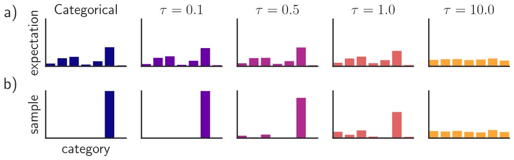
Figure 1: The Gumbel-Softmax distribution interpolates between discrete one-hot-encoded categorical distributions and continuous categorical densities. (a) For low temperatures ($\tau=0.1,\tau=0.5$), the expected value of a Gumbel-Softmax random variable approaches the expected value of a categorical random variable with the same logits. As the temperature increases ($\tau=1.0,\tau=10.0$), the expected value converges to a uniform distribution over the categories. (b) Samples from Gumbel-Softmax distributions are identical to samples from a categorical distribution as $\tau\to 0$. At higher temperatures, Gumbel-Softmax samples are no longer one-hot, and become uniform as $\tau\to\infty$.

图 1：Gumbel-Softmax 分布在离散的 one-hot 类别分布与连续的类别密度之间插值。(a) 在低温下（$\tau=0.1,\tau=0.5$），Gumbel-Softmax 随机变量的期望接近具有相同 logits 的类别随机变量的期望。随着温度升高（$\tau=1.0,\tau=10.0$），期望收敛到各类别上的均匀分布。(b) 当 $\tau\to 0$ 时，Gumbel-Softmax 样本与类别分布样本相同。在更高温度下，样本不再是 one-hot，并在 $\tau\to\infty$ 时趋于均匀。

2.1 Gumbel-Softmax Estimator

2.1 Gumbel-Softmax 估计器

The Gumbel-Softmax distribution is smooth for $\tau>0$, and therefore has a well-defined gradient $\nicefrac{{\partial y}}{{\partial\pi}}$ with respect to the parameters $\pi$. Thus, by replacing categorical samples with Gumbel-Softmax samples we can use backpropagation to compute gradients (see Section 3.1). We denote this procedure of replacing non-differentiable categorical samples with a differentiable approximation during training as the Gumbel-Softmax estimator.

Gumbel-Softmax 分布在 $\tau>0$ 时是光滑的，因此对参数 $\pi$ 有定义良好的梯度 $\nicefrac{{\partial y}}{{\partial\pi}}$。于是，用 Gumbel-Softmax 样本替换类别样本后，就可以用反向传播计算梯度（见第 3.1 节）。我们把训练时用可微近似替换不可微类别样本的这一做法，称为 Gumbel-Softmax 估计器。

While Gumbel-Softmax samples are differentiable, they are not identical to samples from the corresponding categorical distribution for non-zero temperature. For learning, there is a tradeoff between small temperatures, where samples are close to one-hot but the variance of the gradients is large, and large temperatures, where samples are smooth but the variance of the gradients is small (Figure 1). In practice, we start at a high temperature and anneal to a small but non-zero temperature.

尽管 Gumbel-Softmax 样本可微，但在温度非零时，它们并不等同于相应类别分布中的样本。对学习而言，低温与高温之间存在权衡：温度较小时样本接近 one-hot，但梯度方差较大；温度较大时样本更光滑，梯度方差较小（图 1）。实践中，我们从较高温度出发，退火到一个仍大于零的小温度。

In our experiments, we find that the softmax temperature $\tau$ can be annealed according to a variety of schedules and still perform well. If $\tau$ is a learned parameter (rather than annealed via a fixed schedule), this scheme can be interpreted as entropy regularization (Szegedy et al., 2015; Pereyra et al., 2016), where the Gumbel-Softmax distribution can adaptively adjust the “confidence” of proposed samples during the training process.

在实验中，我们发现 softmax 温度 $\tau$ 可以按多种日程退火，并且仍然表现良好。如果 $\tau$ 是一个学习得到的参数（而不是按固定日程退火），这一方案可以理解为熵正则化（Szegedy et al., 2015; Pereyra et al., 2016），此时 Gumbel-Softmax 分布可以在训练过程中自适应地调整所提样本的“置信度”。

2.2 Straight-Through Gumbel-Softmax Estimator

2.2 Straight-Through Gumbel-Softmax 估计器

Continuous relaxations of one-hot vectors are suitable for problems such as learning hidden representations and sequence modeling. For scenarios in which we are constrained to sampling discrete values (e.g. from a discrete action space for reinforcement learning, or quantized compression), we discretize $y$ using $\argmax$ but use our continuous approximation in the backward pass by approximating $\nabla_{\theta}z\approx\nabla_{\theta}y$. We call this the Straight-Through (ST) Gumbel Estimator, as it is reminiscent of the biased path derivative estimator described in Bengio et al. (2013). ST Gumbel-Softmax allows samples to be sparse even when the temperature $\tau$ is high.

one-hot 向量的连续松弛适合于学习隐表示和序列建模这类问题。在必须采样离散值的情形（例如强化学习中的离散动作空间，或量化压缩），我们用 $\argmax$ 对 $y$ 离散化，但在反向传播中使用连续近似，即用 $\nabla_{\theta}y$ 来近似 $\nabla_{\theta}z$。我们称其为 Straight-Through（ST）Gumbel 估计器，因为它让人想起 Bengio et al. (2013) 中描述的有偏路径导数估计器。即便温度 $\tau$ 较高，ST Gumbel-Softmax 也能让样本保持稀疏。

3 Related Work

3 相关工作

In this section we review existing stochastic gradient estimation techniques for discrete variables (illustrated in Figure 2). Consider a stochastic computation graph (Schulman et al., 2015) with discrete random variable $z$ whose distribution depends on parameter $\theta$, and cost function $f(z)$. The objective is to minimize the expected cost $L(\theta)=\mathbb{E}_{z\sim p_{\theta}(z)}[f(z)]$ via gradient descent, which requires us to estimate $\nabla_{\theta}\mathbb{E}_{z\sim p_{\theta}(z)}[f(z)]$.

本节回顾已有的离散变量随机梯度估计技术（如图 2 所示）。考虑一个随机计算图（Schulman et al., 2015），其中有依赖于参数 $\theta$ 的离散随机变量 $z$，以及代价函数 $f(z)$。目标是通过梯度下降最小化期望代价 $L(\theta)=\mathbb{E}_{z\sim p_{\theta}(z)}[f(z)]$，这要求我们估计 $\nabla_{\theta}\mathbb{E}_{z\sim p_{\theta}(z)}[f(z)]$。

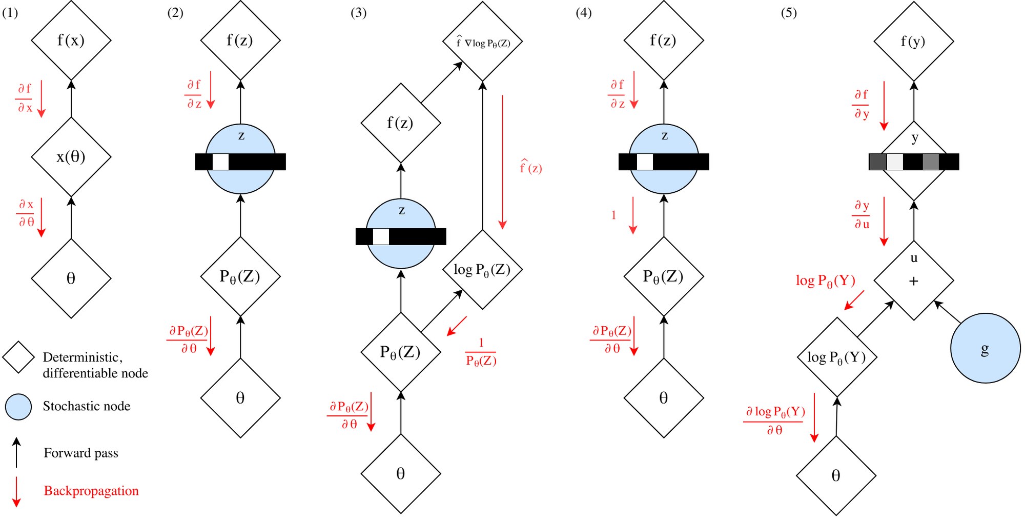
Figure 2: Gradient estimation in stochastic computation graphs. (1) $\nabla_{\theta}{f(x)}$ can be computed via backpropagation if $x(\theta)$ is deterministic and differentiable. (2) The presence of stochastic node $z$ precludes backpropagation as the sampler function does not have a well-defined gradient. (3) The score function estimator and its variants (NVIL, DARN, MuProp, VIMCO) obtain an unbiased estimate of $\nabla_{\theta}{f(x)}$ by backpropagating along a surrogate loss $\hat{f}\log p_{\theta}(z)$, where $\hat{f}=f(x)-b$ and $b$ is a baseline for variance reduction. (4) The Straight-Through estimator, developed primarily for Bernoulli variables, approximates $\nabla_{\theta}z\approx 1$. (5) Gumbel-Softmax is a path derivative estimator for a continuous distribution $y$ that approximates $z$. Reparameterization allows gradients to flow from $f(y)$ to $\theta$. $y$ can be annealed to one-hot categorical variables over the course of training.

图 2：随机计算图中的梯度估计。(1) 如果 $x(\theta)$ 是确定且可微的，则 $\nabla_{\theta}{f(x)}$ 可以通过反向传播计算。(2) 随机节点 $z$ 的出现使反向传播无法进行，因为采样函数没有定义良好的梯度。(3) 得分函数估计器及其变体（NVIL、DARN、MuProp、VIMCO）沿着替代损失 $\hat{f}\log p_{\theta}(z)$ 做反向传播，得到 $\nabla_{\theta}{f(x)}$ 的无偏估计，其中 $\hat{f}=f(x)-b$，$b$ 是用于方差缩减的基线。(4) 主要为伯努利变量发展的 Straight-Through 估计器，近似 $\nabla_{\theta}z\approx 1$。(5) Gumbel-Softmax 是对逼近 $z$ 的连续分布 $y$ 的路径导数估计器。重参数化使梯度可以从 $f(y)$ 流向 $\theta$。在训练过程中，$y$ 可以退火成 one-hot 类别变量。

3.1 Path Derivative Gradient Estimators

3.1 路径导数梯度估计器

For distributions that are reparameterizable, we can compute the sample $z$ as a deterministic function $g$ of the parameters $\theta$ and an independent random variable $\epsilon$, so that $z=g(\theta,\epsilon)$. The path-wise gradients from $f$ to $\theta$ can then be computed without encountering any stochastic nodes:

对于可重参数化的分布，我们可以把样本 $z$ 写成参数 $\theta$ 与一个独立随机变量 $\epsilon$ 的确定性函数 $g$，即 $z=g(\theta,\epsilon)$。于是从 $f$ 到 $\theta$ 的路径梯度可以在不经过任何随机节点的情况下计算：

$$\frac{\partial}{\partial\theta}\mathbb{E}_{z\sim p_{\theta}}\left[f(z))\right]=\frac{\partial}{\partial\theta}\mathbb{E}_{\epsilon}\left[f(g(\theta,\epsilon))\right]=\mathbb{E}_{\epsilon\sim p_{\epsilon}}\left[\frac{\partial f}{\partial g}\frac{\partial g}{\partial\theta}\right] \tag{4}$$

For example, the normal distribution $z\sim\mathcal{N}(\mu,\sigma)$ can be re-written as $\mu+\sigma\cdot\mathcal{N}(0,1)$, making it trivial to compute $\nicefrac{{\partial z}}{{\partial\mu}}$ and $\nicefrac{{\partial z}}{{\partial\sigma}}$. This reparameterization trick is commonly applied to training variational autooencoders with continuous latent variables using backpropagation (Kingma & Welling, 2013; Rezende et al., 2014b). As shown in Figure 2, we exploit such a trick in the construction of the Gumbel-Softmax estimator.

例如，正态分布 $z\sim\mathcal{N}(\mu,\sigma)$ 可以改写成 $\mu+\sigma\cdot\mathcal{N}(0,1)$，从而很容易计算 $\nicefrac{{\partial z}}{{\partial\mu}}$ 和 $\nicefrac{{\partial z}}{{\partial\sigma}}$。这一重参数化技巧常被用于用反向传播训练带有连续潜变量的变分自编码器（Kingma & Welling, 2013; Rezende et al., 2014b）。如图 2 所示，我们在构造 Gumbel-Softmax 估计器时也利用了这一技巧。

Biased path derivative estimators can be utilized even when $z$ is not reparameterizable. In general, we can approximate $\nabla_{\theta}z\approx\nabla_{\theta}m(\theta)$, where $m$ is a differentiable proxy for the stochastic sample. For Bernoulli variables with mean parameter $\theta$, the Straight-Through (ST) estimator (Bengio et al., 2013) approximates $m=\mu_{\theta}(z)$, implying $\nabla_{\theta}m=1$. For $k=2$ (Bernoulli), ST Gumbel-Softmax is similar to the slope-annealed Straight-Through estimator proposed by Chung et al. (2016), but uses a softmax instead of a hard sigmoid to determine the slope. Rolfe (2016) considers an alternative approach where each binary latent variable parameterizes a continuous mixture model. Reparameterization gradients are obtained by backpropagating through the continuous variables and marginalizing out the binary variables.

即便 $z$ 不可重参数化，也可以使用有偏的路径导数估计器。一般地，我们可以近似 $\nabla_{\theta}z\approx\nabla_{\theta}m(\theta)$，其中 $m$ 是随机样本的可微代理。对均值为 $\theta$ 的伯努利变量，Straight-Through（ST）估计器（Bengio et al., 2013）取 $m=\mu_{\theta}(z)$，从而 $\nabla_{\theta}m=1$。当 $k=2$（伯努利）时，ST Gumbel-Softmax 类似于 Chung et al. (2016) 提出的斜坡退火 Straight-Through 估计器，但用 softmax 而不是硬 sigmoid 来确定斜率。Rolfe (2016) 考虑了另一种做法：每个二值潜变量参数化一个连续混合模型。通过对连续变量反向传播并对二值变量边缘化，得到重参数化梯度。

One limitation of the ST estimator is that backpropagating with respect to the sample-independent mean may cause discrepancies between the forward and backward pass, leading to higher variance. Gumbel-Softmax avoids this problem because each sample $y$ is a differentiable proxy of the corresponding discrete sample $z$.

ST 估计器的一个局限是，沿着与样本无关的均值做反向传播，可能导致前向与反向不一致，从而带来更高的方差。Gumbel-Softmax 避免了这一问题，因为每个样本 $y$ 都是相应离散样本 $z$ 的可微代理。

3.2 Score Function-Based Gradient Estimators

3.2 基于得分函数的梯度估计器

The score function estimator (SF, also referred to as REINFORCE (Williams, 1992) and likelihood ratio estimator (Glynn, 1990)) uses the identity $\nabla_{\theta}p_{\theta}(z)=p_{\theta}(z)\nabla_{\theta}\log p_{\theta}(z)$ to derive the following unbiased estimator:

得分函数估计器（SF，也称为 REINFORCE（Williams, 1992）和似然比估计器（Glynn, 1990））利用恒等式 $\nabla_{\theta}p_{\theta}(z)=p_{\theta}(z)\nabla_{\theta}\log p_{\theta}(z)$，得到如下无偏估计器：

$$\nabla_{\theta}\mathbb{E}_{z}\left[f(z)\right]=\mathbb{E}_{z}\left[f(z)\nabla_{\theta}\log p_{\theta}(z)\right] \tag{5}$$

SF only requires that $p_{\theta}(z)$ is continuous in $\theta$, and does not require backpropagating through $f$ or the sample $z$. However, SF suffers from high variance and is consequently slow to converge. In particular, the variance of SF scales linearly with the number of dimensions of the sample vector (Rezende et al., 2014a), making it especially challenging to use for categorical distributions.

SF 只要求 $p_{\theta}(z)$ 对 $\theta$ 连续，并不要求对 $f$ 或样本 $z$ 做反向传播。然而，SF 的方差很大，因此收敛缓慢。尤其是，SF 的方差随样本向量的维数线性增长（Rezende et al., 2014a），这对类别分布来说特别棘手。

The variance of a score function estimator can be reduced by subtracting a control variate $b(z)$ from the learning signal $f$, and adding back its analytical expectation $\mu_{b}=\mathbb{E}_{z}\left[b(z)\nabla_{\theta}\log p_{\theta}(z)\right]$ to keep the estimator unbiased:

得分函数估计器的方差，可以通过从学习信号 $f$ 中减去一个控制变量 $b(z)$，再把它的解析期望 $\mu_{b}=\mathbb{E}_{z}\left[b(z)\nabla_{\theta}\log p_{\theta}(z)\right]$ 加回去来降低，从而保持估计器无偏：

$$\displaystyle\nabla_{\theta}\mathbb{E}_{z}\left[f(z)\right] \\ \displaystyle=\mathbb{E}_{z}\left[f(z)\nabla_{\theta}\log p_{\theta}(z)+(b(z)\nabla_{\theta}\log p_{\theta}(z)-b(z)\nabla_{\theta}\log p_{\theta}(z))\right] \\ \displaystyle=\mathbb{E}_{z}\left[(f(z)-b(z))\nabla_{\theta}\log p_{\theta}(z)\right]+\mu_{b} \tag{6}$$

We briefly summarize recent stochastic gradient estimators that utilize control variates. We direct the reader to Gu et al. (2016) for further detail on these techniques.

我们简要回顾近年来使用控制变量的随机梯度估计器。关于这些技术的更多细节，请读者参阅 Gu et al. (2016)。

• • NVIL (Mnih & Gregor, 2014) uses two baselines: (1) a moving average $\bar{f}$ of $f$ to center the learning signal, and (2) an input-dependent baseline computed by a 1-layer neural network fitted to $f-\bar{f}$ (a control variate for the centered learning signal itself). Finally, variance normalization divides the learning signal by $\max(1,\sigma_{f})$, where $\sigma_{f}^{2}$ is a moving average of $\text{Var}[f]$.

• NVIL（Mnih & Gregor, 2014）使用两个基线：(1) $f$ 的滑动平均 $\bar{f}$，用来把学习信号中心化；(2) 由一层神经网络拟合 $f-\bar{f}$ 得到的、依赖于输入的基线（这是对已中心化学习信号本身的控制变量）。最后，方差归一化把学习信号除以 $\max(1,\sigma_{f})$，其中 $\sigma_{f}^{2}$ 是 $\text{Var}[f]$ 的滑动平均。

• • DARN (Gregor et al., 2013) uses $b=f(\bar{z})+f^{\prime}(\bar{z})(z-\bar{z})$, where the baseline corresponds to the first-order Taylor approximation of $f(z)$ from $f(\bar{z})$. $z$ is chosen to be $\nicefrac{{1}}{{2}}$ for Bernoulli variables, which makes the estimator biased for non-quadratic $f$, since it ignores the correction term $\mu_{b}$ in the estimator expression.

• DARN（Gregor et al., 2013）使用 $b=f(\bar{z})+f^{\prime}(\bar{z})(z-\bar{z})$，其中基线对应于从 $f(\bar{z})$ 出发对 $f(z)$ 的一阶泰勒近似。对伯努利变量，$z$ 取为 $\nicefrac{{1}}{{2}}$，这使得该估计器对非二次的 $f$ 是有偏的，因为它忽略了估计器表达式中的校正项 $\mu_{b}$。

• • MuProp (Gu et al., 2016) also models the baseline as a first-order Taylor expansion: $b=f(\bar{z})+f^{\prime}(\bar{z})(z-\bar{z})$ and $\mu_{b}=f^{\prime}(\bar{z})\nabla_{\theta}\mathbb{E}_{z}\left[z\right]$. To overcome backpropagation through discrete sampling, a mean-field approximation $f_{MF}(\mu_{\theta}(z))$ is used in place of $f(z)$ to compute the baseline and derive the relevant gradients.

• MuProp（Gu et al., 2016）同样把基线建模为一阶泰勒展开：$b=f(\bar{z})+f^{\prime}(\bar{z})(z-\bar{z})$，且 $\mu_{b}=f^{\prime}(\bar{z})\nabla_{\theta}\mathbb{E}_{z}\left[z\right]$。为克服对离散采样的反向传播，它用平均场近似 $f_{MF}(\mu_{\theta}(z))$ 代替 $f(z)$ 来计算基线并推导相关梯度。

• • VIMCO (Mnih & Rezende, 2016) is a gradient estimator for multi-sample objectives that uses the mean of other samples $b=\nicefrac{{1}}{{m}}\sum_{j\neq i}f(z_{j})$ to construct a baseline for each sample $z_{i}\in z_{1:m}$. We exclude VIMCO from our experiments because we are comparing estimators for single-sample objectives, although Gumbel-Softmax can be easily extended to multi-sample objectives.

• VIMCO（Mnih & Rezende, 2016）是面向多样本目标的梯度估计器，它用其他样本的均值 $b=\nicefrac{{1}}{{m}}\sum_{j\neq i}f(z_{j})$ 为每个样本 $z_{i}\in z_{1:m}$ 构造基线。我们没有把它纳入实验，因为我们比较的是单样本目标的估计器；不过 Gumbel-Softmax 可以很容易地推广到多样本目标。

3.3 Semi-Supervised Generative Models

3.3 半监督生成模型

Semi-supervised learning considers the problem of learning from both labeled data $(x,y)\sim\mathcal{D}_{L}$ and unlabeled data $x\sim\mathcal{D}_{U}$, where $x$ are observations (i.e. images) and $y$ are corresponding labels (e.g. semantic class). For semi-supervised classification, Kingma et al. (2014) propose a variational autoencoder (VAE) whose latent state is the joint distribution over a Gaussian “style” variable $z$ and a categorical “semantic class” variable $y$ (Figure 6, Appendix). The VAE objective trains a discriminative network $q_{\phi}(y|x)$, inference network $q_{\phi}(z|x,y)$, and generative network $p_{\theta}(x|y,z)$ end-to-end by maximizing a variational lower bound on the log-likelihood of the observation under the generative model. For labeled data, the class $y$ is observed, so inference is only done on $z\sim q(z|x,y)$. The variational lower bound on labeled data is given by:

半监督学习考虑的是同时从有标签数据 $(x,y)\sim\mathcal{D}_{L}$ 和无标签数据 $x\sim\mathcal{D}_{U}$ 中学习，其中 $x$ 是观测（例如图像），$y$ 是对应的标签（例如语义类别）。对半监督分类，Kingma et al. (2014) 提出一种变分自编码器（VAE），其潜状态是高斯“风格”变量 $z$ 与类别“语义类”变量 $y$ 的联合分布（图 6，附录）。VAE 目标通过最大化观测在生成模型下的对数似然的变分下界，端到端地训练判别网络 $q_{\phi}(y|x)$、推断网络 $q_{\phi}(z|x,y)$ 和生成网络 $p_{\theta}(x|y,z)$。对有标签数据，类别 $y$ 是观测到的，因此推断只对 $z\sim q(z|x,y)$ 进行。有标签数据上的变分下界为：

$$\log p_{\theta}(x,y)\geq-\mathcal{L}(x,y)=\mathbb{E}_{z\sim q_{\phi}(z|x,y)}\left[\log p_{\theta}(x|y,z)]-KL[q(z|x,y)||p_{\theta}(y)p(z)\right] \tag{8}$$

For unlabeled data, difficulties arise because the categorical distribution is not reparameterizable. Kingma et al. (2014) approach this by marginalizing out $y$ over all classes, so that for unlabeled data, inference is still on $q_{\phi}(z|x,y)$ for each $y$. The lower bound on unlabeled data is:

对无标签数据，困难在于类别分布不可重参数化。Kingma et al. (2014) 的做法是对 $y$ 在所有类别上边缘化，从而对无标签数据，推断仍然是对每个 $y$ 做 $q_{\phi}(z|x,y)$。无标签数据上的下界为：

$$\displaystyle\log p_{\theta}(x)\geq-\mathcal{U}(x) \\ \displaystyle=\mathbb{E}_{z\sim q_{\phi}(y,z|x)}[\log p_{\theta}(x|y,z)+\log p_{\theta}(y)+\log p(z)-q_{\phi}(y,z|x)] \\ \displaystyle=\sum_{y}q_{\phi}(y|x)(-\mathcal{L}(x,y)+\mathcal{H}(q_{\phi}(y|x))) \tag{9}$$

The full maximization objective is:

完整的最大化目标为：

$$\mathcal{J}=\mathbb{E}_{(x,y)\sim\mathcal{D}_{L}}\left[-\mathcal{L}(x,y)\right]+\mathbb{E}_{x\sim\mathcal{D}_{U}}\left[-\mathcal{U}(x)\right]+\alpha\cdot\mathbb{E}_{(x,y)\sim\mathcal{D}_{L}}[\log q_{\phi}(y|x)] \tag{11}$$

where $\alpha$ is the scalar trade-off between the generative and discriminative objectives.

其中 $\alpha$ 是生成目标与判别目标之间的标量权衡系数。

One limitation of this approach is that marginalization over all $k$ class values becomes prohibitively expensive for models with a large number of classes. If $D,I,G$ are the computational cost of sampling from $q_{\phi}(y|x)$, $q_{\phi}(z|x,y)$, and $p_{\theta}(x|y,z)$ respectively, then training the unsupervised objective requires $\mathcal{O}(D+k(I+G))$ for each forward/backward step. In contrast, Gumbel-Softmax allows us to backpropagate through $y\sim q_{\phi}(y|x)$ for single sample gradient estimation, and achieves a cost of $\mathcal{O}(D+I+G)$ per training step. Experimental comparisons in training speed are shown in Figure 5.

这一做法的一个局限是，当类别数 $k$ 很大时，对所有类别取值做边缘化会变得过于昂贵。若 $D$、$I$、$G$ 分别是从 $q_{\phi}(y|x)$、$q_{\phi}(z|x,y)$ 和 $p_{\theta}(x|y,z)$ 采样的计算代价，则训练无监督目标时，每一步前向/反向都需要 $\mathcal{O}(D+k(I+G))$。相比之下，Gumbel-Softmax 允许我们对 $y\sim q_{\phi}(y|x)$ 反向传播以做单样本梯度估计，每一步训练的代价为 $\mathcal{O}(D+I+G)$。训练速度上的实验比较见图 5。

4 Experimental Results

4 实验结果

In our first set of experiments, we compare Gumbel-Softmax and ST Gumbel-Softmax to other stochastic gradient estimators: Score-Function (SF), DARN, MuProp, Straight-Through (ST), and Slope-Annealed ST. Each estimator is evaluated on two tasks: (1) structured output prediction and (2) variational training of generative models. We use the MNIST dataset with fixed binarization for training and evaluation, which is common practice for evaluating stochastic gradient estimators (Salakhutdinov & Murray, 2008; Larochelle & Murray, 2011).

在第一组实验中，我们把 Gumbel-Softmax 和 ST Gumbel-Softmax 与其他随机梯度估计器进行比较：得分函数（SF）、DARN、MuProp、Straight-Through（ST）以及斜坡退火 ST。每个估计器在两项任务上评估：(1) 结构化输出预测；(2) 生成模型的变分训练。我们使用固定二值化的 MNIST 进行训练和评测，这是评估随机梯度估计器的常见做法（Salakhutdinov & Murray, 2008; Larochelle & Murray, 2011）。

Learning rates are chosen from $\{3\mathrm{e}{-5},1\mathrm{e}{-5},3\mathrm{e}{-4},1\mathrm{e}{-4},3\mathrm{e}{-3},1\mathrm{e}{-3}\}$; we select the best learning rate for each estimator using the MNIST validation set, and report performance on the test set. Samples drawn from the Gumbel-Softmax distribution are continuous during training, but are discretized to one-hot vectors during evaluation. We also found that variance normalization was necessary to obtain competitive performance for SF, DARN, and MuProp. We used sigmoid activation functions for binary (Bernoulli) neural networks and softmax activations for categorical variables. Models were trained using stochastic gradient descent with momentum $0.9$.

学习率从 $\{3\mathrm{e}{-5},1\mathrm{e}{-5},3\mathrm{e}{-4},1\mathrm{e}{-4},3\mathrm{e}{-3},1\mathrm{e}{-3}\}$ 中选取；我们在 MNIST 验证集上为每个估计器选择最好的学习率，并报告测试集表现。训练时从 Gumbel-Softmax 分布抽取的样本是连续的，评测时则离散化为 one-hot 向量。我们还发现，要使 SF、DARN 和 MuProp 具有竞争力，方差归一化是必要的。二值（伯努利）神经网络使用 sigmoid 激活，类别变量使用 softmax 激活。模型用带动量 $0.9$ 的随机梯度下降训练。

4.1 Structured Output Prediction with Stochastic Binary Networks

4.1 用随机二值网络做结构化输出预测

The objective of structured output prediction is to predict the lower half of a $28\times 28$ MNIST digit given the top half of the image ($14\times 28$). This is a common benchmark for training stochastic binary networks (SBN) (Raiko et al., 2014; Gu et al., 2016; Mnih & Rezende, 2016). The minimization objective for this conditional generative model is an importance-sampled estimate of the likelihood objective, $\mathbb{E}_{h\sim p_{\theta}(h_{i}|x_{\text{upper}})}\left[\frac{1}{m}\sum_{i=1}^{m}\log p_{\theta}(x_{\text{lower}}|h_{i})\right]$, where $m=1$ is used for training and $m=1000$ is used for evaluation.

结构化输出预测的目标，是在给定 $28\times 28$ MNIST 数字上半部分（$14\times 28$）的条件下，预测下半部分。这是训练随机二值网络（SBN）的常见基准（Raiko et al., 2014; Gu et al., 2016; Mnih & Rezende, 2016）。这一条件生成模型的最小化目标，是似然目标的重要性采样估计 $\mathbb{E}_{h\sim p_{\theta}(h_{i}|x_{\text{upper}})}\left[\frac{1}{m}\sum_{i=1}^{m}\log p_{\theta}(x_{\text{lower}}|h_{i})\right]$，训练时取 $m=1$，评测时取 $m=1000$。

We trained a SBN with two hidden layers of 200 units each. This corresponds to either 200 Bernoulli variables (denoted as $392$-$200$-$200$-$392$) or 20 categorical variables (each with 10 classes) with binarized activations (denoted as $392$-$(20\times 10)$-$(20\times 10)$-$392$).

我们训练了一个有两层隐藏层、每层 200 个单元的 SBN。这对应于要么是 200 个伯努利变量（记为 $392$-$200$-$200$-$392$），要么是 20 个类别变量（每个有 10 类）并对其激活做二值化（记为 $392$-$(20\times 10)$-$(20\times 10)$-$392$）。

As shown in Figure 3, ST Gumbel-Softmax is on par with the other estimators for Bernoulli variables and outperforms on categorical variables. Meanwhile, Gumbel-Softmax outperforms other estimators on both Bernoulli and Categorical variables. We found that it was not necessary to anneal the softmax temperature for this task, and used a fixed $\tau=1$.

如图 3 所示，ST Gumbel-Softmax 在伯努利变量上与其他估计器相当，在类别变量上则更优。与此同时，Gumbel-Softmax 在伯努利和类别两种变量上都优于其他估计器。我们发现这一任务不必对 softmax 温度退火，因而使用了固定的 $\tau=1$。

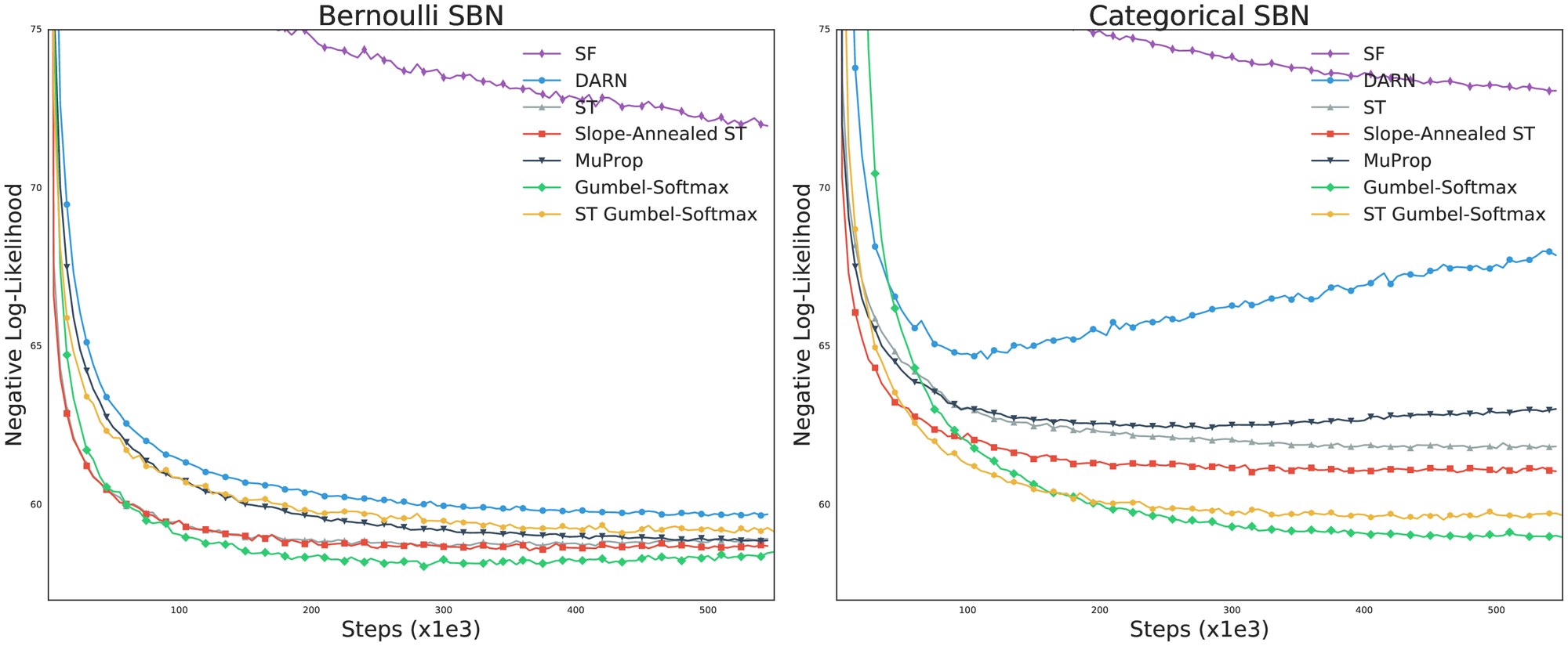
Figure 3: Test loss (negative log-likelihood) on the structured output prediction task with binarized MNIST using a stochastic binary network with (a) Bernoulli latent variables ($392$-$200$-$200$-$392$) and (b) categorical latent variables ($392$-$(20\times 10)$-$(20\times 10)$-$392$).

图 3：在固定二值化 MNIST 上，用随机二值网络做结构化输出预测时的测试损失（负对数似然）。(a) 伯努利潜变量（$392$-$200$-$200$-$392$）；(b) 类别潜变量（$392$-$(20\times 10)$-$(20\times 10)$-$392$）。

4.2 Generative Modeling with Variational Autoencoders

4.2 用变分自编码器做生成建模

We train variational autoencoders (Kingma & Welling, 2013), where the objective is to learn a generative model of binary MNIST images. In our experiments, we modeled the latent variable as a single hidden layer with 200 Bernoulli variables or 20 categorical variables ($20\times 10$). We use a learned categorical prior rather than a Gumbel-Softmax prior in the training objective. Thus, the minimization objective during training is no longer a variational bound if the samples are not discrete. In practice, we find that optimizing this objective in combination with temperature annealing still minimizes actual variational bounds on validation and test sets. Like the structured output prediction task, we use a multi-sample bound for evaluation with $m=1000$.

我们训练变分自编码器（Kingma & Welling, 2013），目标是学习二值 MNIST 图像的生成模型。实验中，我们把潜变量建模为单层隐藏层，其中有 200 个伯努利变量，或 20 个类别变量（$20\times 10$）。在训练目标中，我们使用学习得到的类别先验，而不是 Gumbel-Softmax 先验。因此，若样本不是离散的，训练时的最小化目标便不再是变分界。实践中，我们发现优化这一目标并配合温度退火，仍然能够降低验证集和测试集上真正的变分界。与结构化输出预测任务一样，评测使用 $m=1000$ 的多样本界。

The temperature is annealed using the schedule $\tau=\text{max}(0.5,\text{exp}(-rt))$ of the global training step $t$, where $\tau$ is updated every $N$ steps. $N\in\{500,1000\}$ and $r\in\{1\mathrm{e}{-5},1\mathrm{e}{-4}\}$ are hyperparameters for which we select the best-performing estimator on the validation set and report test performance.

温度按全局训练步 $t$ 的日程 $\tau=\text{max}(0.5,\text{exp}(-rt))$ 退火，每 $N$ 步更新一次 $\tau$。$N\in\{500,1000\}$ 和 $r\in\{1\mathrm{e}{-5},1\mathrm{e}{-4}\}$ 是超参数，我们在验证集上为表现最好的估计器选定它们，并报告测试表现。

As shown in Figure 4, ST Gumbel-Softmax outperforms other estimators for Categorical variables, and Gumbel-Softmax drastically outperforms other estimators in both Bernoulli and Categorical variables.

如图 4 所示，ST Gumbel-Softmax 在类别变量上优于其他估计器，而 Gumbel-Softmax 在伯努利和类别两种变量上都大幅优于其他估计器。

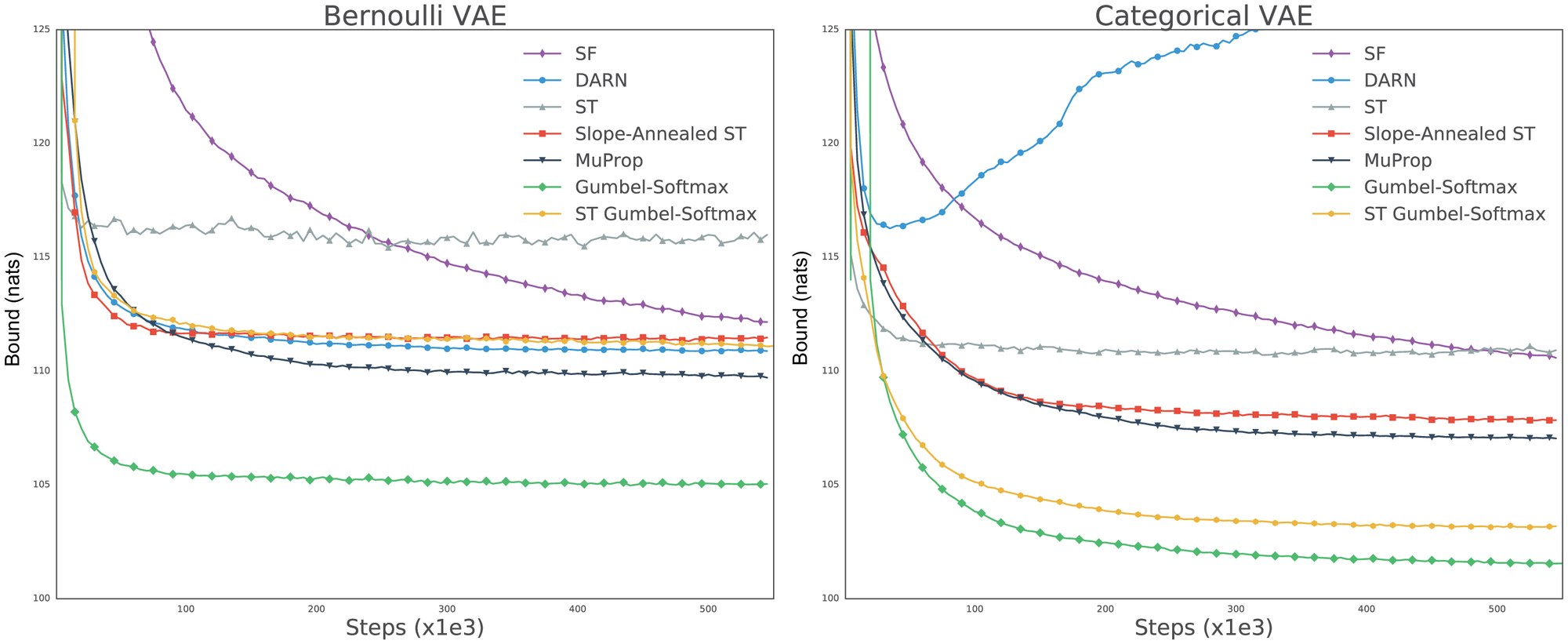
Figure 4: Test loss (negative variational lower bound) on binarized MNIST VAE with (a) Bernoulli latent variables ($784-200-784$) and (b) categorical latent variables ($784-(20\times 10)-200$).

图 4：二值化 MNIST 上 VAE 的测试损失（负变分下界）。(a) 伯努利潜变量（$784-200-784$）；(b) 类别潜变量（$784-(20\times 10)-200$）。

	SF	DARN	MuProp	ST	Annealed ST	Gumbel-S.	ST Gumbel-S.
SBN (Bern.)	72.0	59.7	58.9	58.9	58.7	58.5	59.3
SBN (Cat.)	73.1	67.9	63.0	61.8	61.1	59.0	59.7
VAE (Bern.)	112.2	110.9	109.7	116.0	111.5	105.0	111.5
VAE (Cat.)	110.6	128.8	107.0	110.9	107.8	101.5	107.8

Table 1: The Gumbel-Softmax estimator outperforms other estimators on Bernoulli and Categorical latent variables. For the structured output prediction (SBN) task, numbers correspond to negative log-likelihoods (nats) of input images (lower is better). For the VAE task, numbers correspond to negative variational lower bounds (nats) on the log-likelihood (lower is better).

	SF	DARN	MuProp	ST	Annealed ST	Gumbel-S.	ST Gumbel-S.
SBN（伯努利）	72.0	59.7	58.9	58.9	58.7	58.5	59.3
SBN（类别）	73.1	67.9	63.0	61.8	61.1	59.0	59.7
VAE（伯努利）	112.2	110.9	109.7	116.0	111.5	105.0	111.5
VAE（类别）	110.6	128.8	107.0	110.9	107.8	101.5	107.8

表 1：Gumbel-Softmax 估计器在伯努利和类别潜变量上都优于其他估计器。对结构化输出预测（SBN）任务，数字是输入图像的负对数似然（nats，越低越好）。对 VAE 任务，数字是对数似然的负变分下界（nats，越低越好）。

4.3 Generative Semi-Supervised Classification

4.3 生成式半监督分类

We apply the Gumbel-Softmax estimator to semi-supervised classification on the binary MNIST dataset. We compare the original marginalization-based inference approach (Kingma et al., 2014) to single-sample inference with Gumbel-Softmax and ST Gumbel-Softmax.

我们把 Gumbel-Softmax 估计器用于二值 MNIST 数据集上的半监督分类，并把原先基于边缘化的推断方法（Kingma et al., 2014）与使用 Gumbel-Softmax 和 ST Gumbel-Softmax 的单样本推断加以比较。

We trained on a dataset consisting of 100 labeled examples (distributed evenly among each of the 10 classes) and 50,000 unlabeled examples, with dynamic binarization of the unlabeled examples for each minibatch. The discriminative model $q_{\phi}(y|x)$ and inference model $q_{\phi}(z|x,y)$ are each implemented as 3-layer convolutional neural networks with ReLU activation functions. The generative model $p_{\theta}(x|y,z)$ is a 4-layer convolutional-transpose network with ReLU activations. Experimental details are provided in Appendix A.

我们在由 100 个有标签样本（在 10 个类别中均匀分配）和 50,000 个无标签样本组成的数据集上训练，并对每个小批量的无标签样本做动态二值化。判别模型 $q_{\phi}(y|x)$ 和推断模型 $q_{\phi}(z|x,y)$ 各自实现为带 ReLU 激活的 3 层卷积神经网络。生成模型 $p_{\theta}(x|y,z)$ 是带 ReLU 激活的 4 层转置卷积网络。实验细节见附录 A。

Estimators were trained and evaluated against several values of $\alpha=\{0.1,0.2,0.3,0.8,1.0\}$ and the best unlabeled classification results for test sets were selected for each estimator and reported in Table 2. We used an annealing schedule of $\tau=\text{max}(0.5,\text{exp}(-3\mathrm{e}{-5}\cdot t))$, updated every 2000 steps.

估计器在若干 $\alpha=\{0.1,0.2,0.3,0.8,1.0\}$ 取值下训练和评估，每个估计器选取测试集上最好的无标签分类结果，报告于表 2。我们使用的退火日程为 $\tau=\text{max}(0.5,\text{exp}(-3\mathrm{e}{-5}\cdot t))$，每 2000 步更新一次。

In Kingma et al. (2014), inference over the latent state is done by marginalizing out $y$ and using the reparameterization trick for sampling from $q_{\phi}(z|x,y)$. However, this approach has a computational cost that scales linearly with the number of classes. Gumbel-Softmax allows us to backpropagate directly through single samples from the joint $q_{\phi}(y,z|x)$, achieving drastic speedups in training without compromising generative or classification performance. (Table 2, Figure 5).

在 Kingma et al. (2014) 中，对潜状态的推断是通过对 $y$ 边缘化、并对 $q_{\phi}(z|x,y)$ 的采样使用重参数化技巧完成的。然而，这一做法的计算代价随类别数线性增长。Gumbel-Softmax 使我们能够直接对来自联合分布 $q_{\phi}(y,z|x)$ 的单次样本反向传播，从而在不牺牲生成或分类性能的前提下，大幅加快训练（表 2，图 5）。

	ELBO	Accuracy
Marginalization	-106.8	92.6%
Gumbel	-109.6	92.4%
ST Gumbel-Softmax	-110.7	93.6%

Table 2: Marginalizing over $y$ and single-sample variational inference perform equally well when applied to image classification on the binarized MNIST dataset (Larochelle & Murray, 2011). We report variational lower bounds and image classification accuracy for unlabeled data in the test set.

	ELBO	准确率
边缘化	-106.8	92.6%
Gumbel	-109.6	92.4%
ST Gumbel-Softmax	-110.7	93.6%

表 2：在二值化 MNIST 数据集（Larochelle & Murray, 2011）的图像分类上，对 $y$ 做边缘化与单样本变分推断的表现相当。我们报告测试集中无标签数据的变分下界和图像分类准确率。

In Figure 5, we show how Gumbel-Softmax versus marginalization scales with the number of categorical classes. For these experiments, we use MNIST images with randomly generated labels. Training the model with the Gumbel-Softmax estimator is $2\times$ as fast for $10$ classes and $9.9\times$ as fast for $100$ classes.

在图 5 中，我们展示 Gumbel-Softmax 相对边缘化如何随类别数扩展。这些实验使用带有随机生成标签的 MNIST 图像。用 Gumbel-Softmax 估计器训练模型时，10 类大约快 $2\times$，100 类大约快 $9.9\times$。

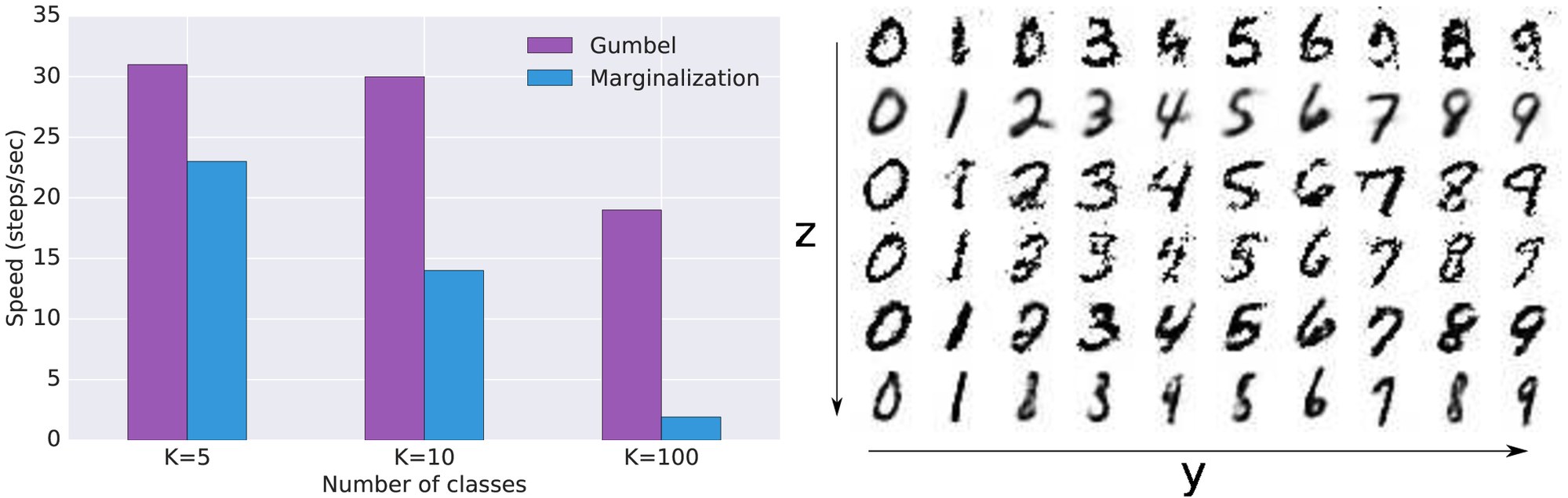
Figure 5: Gumbel-Softmax allows us to backpropagate through samples from the posterior $q_{\phi}(y|x)$, providing a scalable method for semi-supervised learning for tasks with a large number of classes. (a) Comparison of training speed (steps/sec) between Gumbel-Softmax and marginalization (Kingma et al., 2014) on a semi-supervised VAE. Evaluations were performed on a GTX Titan X® GPU. (b) Visualization of MNIST analogies generated by varying style variable $z$ across each row and class variable $y$ across each column.

图 5：Gumbel-Softmax 允许我们对来自后验 $q_{\phi}(y|x)$ 的样本反向传播，从而为类别数较多的任务提供一种可扩展的半监督学习方法。(a) 半监督 VAE 上 Gumbel-Softmax 与边缘化（Kingma et al., 2014）的训练速度（步/秒）比较。评测在一块 GTX Titan X® GPU 上进行。(b) 通过沿每行改变风格变量 $z$、沿每列改变类别变量 $y$ 生成的 MNIST 类比可视化。

5 Discussion

5 讨论

The primary contribution of this work is the reparameterizable Gumbel-Softmax distribution, whose corresponding estimator affords low-variance path derivative gradients for the categorical distribution. We show that Gumbel-Softmax and Straight-Through Gumbel-Softmax are effective on structured output prediction and variational autoencoder tasks, outperforming existing stochastic gradient estimators for both Bernoulli and categorical latent variables. Finally, Gumbel-Softmax enables dramatic speedups in inference over discrete latent variables.

本文的主要贡献是可重参数化的 Gumbel-Softmax 分布，与之对应的估计器为类别分布提供了低方差的路径导数梯度。我们表明，Gumbel-Softmax 和 Straight-Through Gumbel-Softmax 在结构化输出预测和变分自编码器任务上是有效的，在伯努利和类别潜变量上都优于已有的随机梯度估计器。最后，Gumbel-Softmax 使对离散潜变量的推断获得了显著加速。

Acknowledgments

We sincerely thank Luke Vilnis, Vincent Vanhoucke, Luke Metz, David Ha, Laurent Dinh, George Tucker, and Subhaneil Lahiri for helpful discussions and feedback.

致谢

我们衷心感谢 Luke Vilnis、Vincent Vanhoucke、Luke Metz、David Ha、Laurent Dinh、George Tucker 和 Subhaneil Lahiri 的有益讨论与反馈。

References

参考文献

Bengio et al. (2013) Y. Bengio, N. Léonard, and A. Courville. Estimating or propagating gradients through stochastic neurons for conditional computation. arXiv preprint arXiv:1308.3432 , 2013.

Chen et al. (2016) Xi Chen, Yan Duan, Rein Houthooft, John Schulman, Ilya Sutskever, and Pieter Abbeel. Infogan: Interpretable representation learning by information maximizing generative adversarial nets. CoRR , abs/1606.03657, 2016.

Chung et al. (2016) J. Chung, S. Ahn, and Y. Bengio. Hierarchical multiscale recurrent neural networks. arXiv preprint arXiv:1609.01704 , 2016.

Glynn (1990) P. W Glynn. Likelihood ratio gradient estimation for stochastic systems. Communications of the ACM , 33(10):75–84, 1990.

Graves et al. (2016) A. Graves, G. Wayne, M. Reynolds, T. Harley, I. Danihelka, A. Grabska-Barwińska, S. G. Colmenarejo, E. Grefenstette, T. Ramalho, J. Agapiou, et al. Hybrid computing using a neural network with dynamic external memory. Nature , 538(7626):471–476, 2016.

Graves et al. (2014) Alex Graves, Greg Wayne, and Ivo Danihelka. Neural turing machines. CoRR , abs/1410.5401, 2014.

Gregor et al. (2013) K. Gregor, I. Danihelka, A. Mnih, C. Blundell, and D. Wierstra. Deep autoregressive networks. arXiv preprint arXiv:1310.8499 , 2013.

Gu et al. (2016) S. Gu, S. Levine, I. Sutskever, and A Mnih. MuProp: Unbiased Backpropagation for Stochastic Neural Networks. ICLR , 2016.

Gumbel (1954) E. J. Gumbel. Statistical theory of extreme values and some practical applications: a series of lectures . Number 33. US Govt. Print. Office, 1954.

Kingma & Welling (2013) D. P. Kingma and M. Welling. Auto-encoding variational bayes. arXiv preprint arXiv:1312.6114 , 2013.

Kingma et al. (2014) D. P. Kingma, S. Mohamed, D. J. Rezende, and M. Welling. Semi-supervised learning with deep generative models. In Advances in Neural Information Processing Systems , pp. 3581–3589, 2014.

Larochelle & Murray (2011) H. Larochelle and I. Murray. The neural autoregressive distribution estimator. In AISTATS , volume 1, pp.  2, 2011.

Maddison et al. (2014) C. J. Maddison, D. Tarlow, and T. Minka. A* sampling. In Advances in Neural Information Processing Systems , pp. 3086–3094, 2014.

Maddison et al. (2016) C. J. Maddison, A. Mnih, and Y. Whye Teh. The Concrete Distribution: A Continuous Relaxation of Discrete Random Variables. ArXiv e-prints , November 2016.

Mnih & Gregor (2014) A. Mnih and K. Gregor. Neural variational inference and learning in belief networks. ICML , 31, 2014.

Mnih & Rezende (2016) A. Mnih and D. J. Rezende. Variational inference for monte carlo objectives. arXiv preprint arXiv:1602.06725 , 2016.

Paisley et al. (2012) J. Paisley, D. Blei, and M. Jordan. Variational Bayesian Inference with Stochastic Search. ArXiv e-prints , June 2012.

Pereyra et al. (2016) Gabriel Pereyra, Geoffrey Hinton, George Tucker, and Lukasz Kaiser. Regularizing neural networks by penalizing confident output distributions. 2016.

Rae et al. (2016) J. W Rae, J. J Hunt, T. Harley, I. Danihelka, A. Senior, G. Wayne, A. Graves, and T. P Lillicrap. Scaling Memory-Augmented Neural Networks with Sparse Reads and Writes. ArXiv e-prints , October 2016.

Raiko et al. (2014) T. Raiko, M. Berglund, G. Alain, and L. Dinh. Techniques for learning binary stochastic feedforward neural networks. arXiv preprint arXiv:1406.2989 , 2014.

Rezende et al. (2014a) D. J. Rezende, S. Mohamed, and D. Wierstra. Stochastic backpropagation and approximate inference in deep generative models. arXiv preprint arXiv:1401.4082 , 2014a.

Rezende et al. (2014b) D. J. Rezende, S. Mohamed, and D. Wierstra. Stochastic backpropagation and approximate inference in deep generative models. In Proceedings of The 31st International Conference on Machine Learning , pp. 1278–1286, 2014b.

Rolfe (2016) J. T. Rolfe. Discrete Variational Autoencoders. ArXiv e-prints , September 2016.

Salakhutdinov & Murray (2008) R. Salakhutdinov and I. Murray. On the quantitative analysis of deep belief networks. In Proceedings of the 25th international conference on Machine learning , pp. 872–879. ACM, 2008.

Schulman et al. (2015) J. Schulman, N. Heess, T. Weber, and P. Abbeel. Gradient estimation using stochastic computation graphs. In Advances in Neural Information Processing Systems , pp. 3528–3536, 2015.

Szegedy et al. (2015) C. Szegedy, V. Vanhoucke, S. Ioffe, J. Shlens, and Z. Wojna. Rethinking the inception architecture for computer vision. arXiv preprint arXiv:1512.00567 , 2015.

Williams (1992) R. J. Williams. Simple statistical gradient-following algorithms for connectionist reinforcement learning. Machine learning , 8(3-4):229–256, 1992.

Xu et al. (2015) K. Xu, J. Ba, R. Kiros, K. Cho, A. C. Courville, R. Salakhutdinov, R. S. Zemel, and Y. Bengio. Show, attend and tell: Neural image caption generation with visual attention. CoRR , abs/1502.03044, 2015.

Appendix A Semi-Supervised Classification Model

附录 A 半监督分类模型

Figures 6 and 7 describe the architecture used in our experiments for semi-supervised classification (Section 4.3).

图 6 和图 7 描述了我们在半监督分类实验中使用的结构（第 4.3 节）。

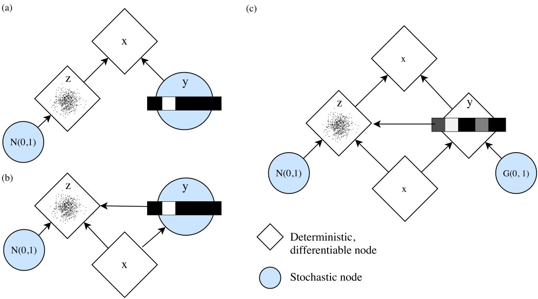
Figure 6: Semi-supervised generative model proposed by Kingma et al. (2014). (a) Generative model $p_{\theta}(x|y,z)$ synthesizes images from latent Gaussian “style” variable $z$ and categorical class variable $y$. (b) Inference model $q_{\phi}(y,z|x)$ samples latent state $y,z$ given $x$. Gaussian $z$ can be differentiated with respect to its parameters because it is reparameterizable. In previous work, when $y$ is not observed, training the VAE objective requires marginalizing over all values of $y$. (c) Gumbel-Softmax reparameterizes $y$ so that backpropagation is also possible through $y$ without encountering stochastic nodes.

图 6：Kingma et al. (2014) 提出的半监督生成模型。(a) 生成模型 $p_{\theta}(x|y,z)$ 从潜在的高斯“风格”变量 $z$ 和类别变量 $y$ 合成图像。(b) 推断模型 $q_{\phi}(y,z|x)$ 在给定 $x$ 时采样潜状态 $y,z$。高斯变量 $z$ 对其参数可微，因为它是可重参数化的。在以往工作中，当 $y$ 未被观测时，训练 VAE 目标需要对 $y$ 的所有取值做边缘化。(c) Gumbel-Softmax 对 $y$ 做重参数化，从而使反向传播也可以穿过 $y$ 而不遇到随机节点。

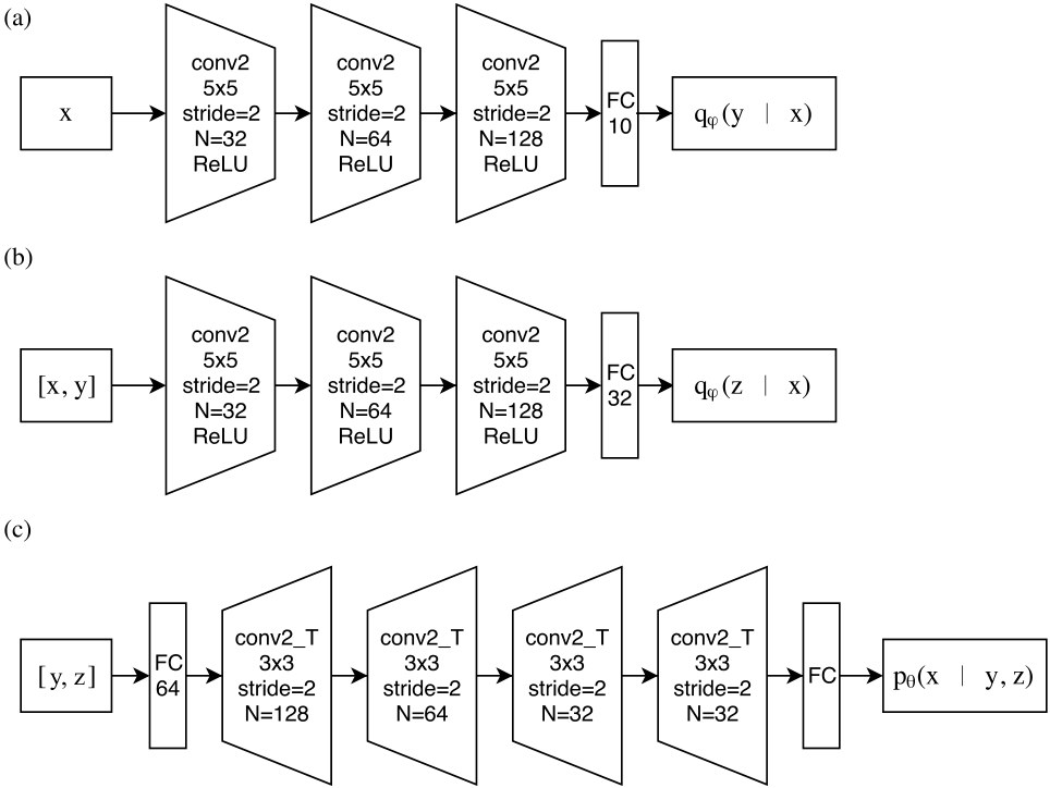
Figure 7: Network architecture for (a) classification $q_{\phi}(y|x)$ (b) inference $q_{\phi}(z|x,y)$, and (c) generative $p_{\theta}(x|y,z)$ models. The output of these networks parameterize Categorical, Gaussian, and Bernoulli distributions which we sample from.

图 7：(a) 分类 $q_{\phi}(y|x)$、(b) 推断 $q_{\phi}(z|x,y)$ 和 (c) 生成 $p_{\theta}(x|y,z)$ 模型的网络结构。这些网络的输出分别参数化我们从中采样的类别、高斯和伯努利分布。

Appendix B Deriving the density of the Gumbel-Softmax distribution

附录 B 推导 Gumbel-Softmax 分布的密度

Here we derive the probability density function of the Gumbel-Softmax distribution with probabilities $\pi_{1},...,\pi_{k}$ and temperature $\tau$. We first define the logits $x_{i}=\log\pi_{i}$, and Gumbel samples $g_{1},...,g_{k}$, where $g_{i}\sim\text{Gumbel}(0,1)$. A sample from the Gumbel-Softmax can then be computed as:

这里我们推导具有概率 $\pi_{1},...,\pi_{k}$ 和温度 $\tau$ 的 Gumbel-Softmax 分布的概率密度函数。首先定义 logits $x_{i}=\log\pi_{i}$，以及 Gumbel 样本 $g_{1},...,g_{k}$，其中 $g_{i}\sim\text{Gumbel}(0,1)$。于是 Gumbel-Softmax 的一个样本可以计算为：

$$y_{i}=\frac{\exp\left((x_{i}+g_{i})/\tau\right)}{\sum_{j=1}^{k}\exp\left((x_{j}+g_{j})/\tau\right)}\qquad\text{for }i=1,...,k \tag{12}$$

B.1 Centered Gumbel density

B.1 中心化 Gumbel 密度

The mapping from the Gumbel samples $g$ to the Gumbel-Softmax sample $y$ is not invertible as the normalization of the softmax operation removes one degree of freedom. To compensate for this, we define an equivalent sampling process that subtracts off the last element, $(x_{k}+g_{k})/\tau$ before the softmax:

从 Gumbel 样本 $g$ 到 Gumbel-Softmax 样本 $y$ 的映射不是可逆的，因为 softmax 的归一化去掉了一个自由度。为补偿这一点，我们定义一个等价的采样过程：在 softmax 之前减去最后一项 $(x_{k}+g_{k})/\tau$：

$$y_{i}=\frac{\exp\left((x_{i}+g_{i}-(x_{k}+g_{k}))/\tau\right)}{\sum_{j=1}^{k}\exp\left((x_{j}+g_{j}-(x_{k}+g_{k}))/\tau\right)}\qquad\text{for }i=1,...,k \tag{13}$$

To derive the density of this equivalent sampling process, we first derive the density for the ”centered” multivariate Gumbel density corresponding to:

为推导这一等价采样过程的密度，我们首先推导对应于下式的“中心化”多元 Gumbel 密度：

$$u_{i}=x_{i}+g_{i}-(x_{k}+g_{k})\qquad\text{for }i=1,...,k-1 \tag{14}$$

where $g_{i}\sim\text{Gumbel}(0,1)$. Note the probability density of a Gumbel distribution with scale parameter $\beta=1$ and mean $\mu$ at $z$ is: $f(z,\mu)=e^{\mu-z-e^{\mu-z}}$. We can now compute the density of this distribution by marginalizing out the last Gumbel sample, $g_{k}$:

其中 $g_{i}\sim\text{Gumbel}(0,1)$。注意，尺度参数 $\beta=1$、均值为 $\mu$ 的 Gumbel 分布在 $z$ 处的概率密度为：$f(z,\mu)=e^{\mu-z-e^{\mu-z}}$。我们现在可以通过对最后一个 Gumbel 样本 $g_{k}$ 边缘化来计算这一分布的密度：

$$\displaystyle p(u_{1},...,u_{k-1}) \\ \displaystyle=\int_{-\infty}^{\infty}dg_{k}\,p(u_{1},...,u_{k}|g_{k})p(g_{k}) \\ \displaystyle=\int_{-\infty}^{\infty}dg_{k}\,p(g_{k})\prod_{i=1}^{k-1}p(u_{i}|g_{k}) \\ \displaystyle=\int_{-\infty}^{\infty}dg_{k}\,f(g_{k},0)\prod_{i=1}^{k-1}f(x_{k}+g_{k},x_{i}-u_{i}) \\ \displaystyle=\int_{-\infty}^{\infty}dg_{k}\,e^{-g_{k}-e^{-g_{k}}}\prod_{i=1}^{k-1}e^{x_{i}-u_{i}-x_{k}-g_{k}-e^{x_{i}-u_{i}-x_{k}-g_{k}}}$$

We perform a change of variables with $v=e^{-g_{k}}$, so $dv=-e^{-g_{k}}dg_{k}$ and $dg_{k}=-dv\,e^{g_{k}}=dv/v$, and define $u_{k}=0$ to simplify notation:

我们做变量替换 $v=e^{-g_{k}}$，于是 $dv=-e^{-g_{k}}dg_{k}$，$dg_{k}=-dv\,e^{g_{k}}=dv/v$，并定义 $u_{k}=0$ 以简化记号：

$$\displaystyle p(u_{1},...,u_{k,-1}) \\ \displaystyle=\delta(u_{k}=0)\int_{0}^{\infty}dv\,\frac{1}{v}ve^{x_{k}-v}\prod_{i=1}^{k-1}ve^{x_{i}-u_{i}-x_{k}-ve^{x_{i}-u_{i}-x_{k}}} \\ \displaystyle=\exp\left(x_{k}+\sum_{i=1}^{k-1}(x_{i}-u_{i})\right)\left(e^{x_{k}}+\sum_{i=1}^{k-1}\left(e^{x_{i}-u_{i}}\right)\right)^{-k}\Gamma(k) \\ \displaystyle=\Gamma(k)\exp\left(\sum_{i=1}^{k}(x_{i}-u_{i})\right)\left(\sum_{i=1}^{k}\left(e^{x_{i}-u_{i}}\right)\right)^{-k} \\ \displaystyle=\Gamma(k)\left(\prod_{i=1}^{k}\exp\left(x_{i}-u_{i}\right)\right)\left(\sum_{i=1}^{k}\exp\left(x_{i}-u_{i}\right)\right)^{-k} \tag{15}$$

B.2 Transforming to a Gumbel-Softmax

B.2 变换到 Gumbel-Softmax

Given samples $u_{1},...,u_{k,-1}$ from the centered Gumbel distribution, we can apply a deterministic transformation $h$ to yield the first $k-1$ coordinates of the sample from the Gumbel-Softmax:

给定来自中心化 Gumbel 分布的样本 $u_{1},...,u_{k,-1}$，我们可以施加一个确定性变换 $h$，得到 Gumbel-Softmax 样本的前 $k-1$ 个坐标：

$$y_{1:k-1}=h(u_{1:k-1}),\qquad h_{i}(u_{1:k-1})=\frac{\exp(u_{i}/\tau)}{1+\sum_{j=1}^{k-1}\exp(u_{j}/\tau)}\forall i=1,\dots,{k-1} \tag{19}$$

Note that the final coordinate probability $y_{k}$ is fixed given the first $k-1$, as $\sum_{i=1}^{k}y_{i}=1$:

注意，给定前 $k-1$ 个坐标后，最后的坐标概率 $y_{k}$ 是确定的，因为 $\sum_{i=1}^{k}y_{i}=1$：

$$y_{k}=\left(1+{\sum_{j=1}^{k-1}\exp(u_{j}/\tau)}\right)^{-1}=1-\sum_{j=1}^{k-1}y_{j} \tag{20}$$

We can thus compute the probability of a sample from the Gumbel-Softmax using the change of variables formula on only the first $k-1$ variables:

因此，我们可以只对前 $k-1$ 个变量使用变量替换公式，来计算 Gumbel-Softmax 样本的概率：

$$p(y_{1:k})=p\left(h^{-1}(y_{1:k-1})\right)\text{det}\left(\frac{\partial h^{-1}(y_{1:k-1})}{\partial y_{1:k-1}}\right) \tag{21}$$

Thus we need to compute two more pieces: the inverse of $h$ and its Jacobian determinant. The inverse of $h$ is:

于是还需要计算两样东西：$h$ 的逆及其雅可比行列式。$h$ 的逆为：

$$\displaystyle h^{-1}(y_{1:k-1})=\tau\times\left(\log y_{i}-\log\left(1-\sum_{j=1}^{k-1}y_{j}\right)\right)=\tau\times\left(\log y_{i}-\log y_{k}\right) \tag{22}$$

with Jacobian

其雅可比为

$$\frac{\partial h^{-1}(y_{1:k-1})}{\partial y_{1:k-1}}=\tau\times\left(\text{diag}\left(\frac{1}{y_{1:k-1}}\right)+\frac{1}{y_{k}}\right)=\begin{bmatrix}\frac{1}{y_{1}}+\frac{1}{y_{k}}&\frac{1}{y_{k}}&\dots&\frac{1}{y_{k}}\
\frac{1}{y_{k}}&\frac{1}{y_{2}}+\frac{1}{y_{k}}&\dots&\frac{1}{y_{k}}\
\vdots&\vdots&\ddots&\vdots\
\frac{1}{y_{k}}&\frac{1}{y_{k}}&\dots&\frac{1}{y_{k-1}}+\frac{1}{y_{k}}\end{bmatrix} \tag{23}$$

Next, we compute the determinant of the Jacobian:

接下来，我们计算雅可比的行列式：

$$\displaystyle\text{det}\left(\frac{\partial h^{-1}(y_{1:k-1})}{\partial y_{1:k-1}}\right) \\ \displaystyle=\tau^{k-1}\text{det}\left(\left(I+\frac{1}{y_{k}}ee^{T}\text{diag}\left(y_{1:k-1}\right)\right)\left(\text{diag}\left(\frac{1}{y_{1:k-1}}\right)\right)\right) \\ \displaystyle=\tau^{k-1}\left(1+\frac{1-y_{k}}{y_{k}}\right)\prod_{j=1}^{k-1}y_{j}^{-1} \\ \displaystyle=\tau^{k-1}\prod_{j=1}^{k}y_{j}^{-1} \tag{24}$$

where $e$ is a $k-1$ dimensional vector of ones, and we’ve used the identities: $\text{det}(AB)=\text{det}(A)\text{det}(B)$, $\text{det}(\text{diag}(x))=\prod_{i}x_{i}$, and $\text{det}(I+uv^{T})=1+u^{T}v$.

其中 $e$ 是 $k-1$ 维的全 1 向量，并且我们使用了恒等式：$\text{det}(AB)=\text{det}(A)\text{det}(B)$，$\text{det}(\text{diag}(x))=\prod_{i}x_{i}$，以及 $\text{det}(I+uv^{T})=1+u^{T}v$。

We can then plug into the change of variables formula (Eq. 21) using the density of the centered Gumbel (Eq.15), the inverse of $h$ (Eq. 22) and its Jacobian determinant (Eq. 26):

然后我们可以把中心化 Gumbel 的密度（式 15）、$h$ 的逆（式 22）及其雅可比行列式（式 26）代入变量替换公式（式 21）：

$$\displaystyle p(y_{1},..,y_{k}) \\ \displaystyle=\Gamma(k)\left(\prod_{i=1}^{k}\exp\left(x_{i}\right)\frac{y_{k}^{\tau}}{y_{i}^{\tau}}\right)\left(\sum_{i=1}^{k}\exp\left(x_{i}\right)\frac{y_{k}^{\tau}}{y_{i}^{\tau}}\right)^{-k}\tau^{k-1}\prod_{i=1}^{k}y_{i}^{-1} \\ \displaystyle=\Gamma(k)\tau^{k-1}\left(\sum_{i=1}^{k}\exp\left(x_{i}\right)/{y_{i}^{\tau}}\right)^{-k}\prod_{i=1}^{k}\left(\exp\left(x_{i}\right)/y_{i}^{\tau+1}\right) \tag{27}$$