To Grok Grokking: Provable Grokking in Ridge Regression
To Grok Grokking: Provable Grokking in Ridge Regression
To Grok Grokking:岭回归中可证明的 Grokking
Mingyue Xu Affiliation: Department of Computer Science, Purdue University, West Lafayette, IN, USA Correspondence to: xu1864@purdue.edu Gal Vardi Affiliation: Department of Computer Science and Applied Mathematics, Weizmann Institute of Science, Israel Itay Safran Affiliation: Stein Faculty of Computer and Information Science, Ben-Gurion University of the Negev, Israel
Abstract
摘要
We study grokking—the onset of generalization long after overfitting—in a classical ridge regression setting. We prove end-to-end grokking results for learning over-parameterized linear regression models using gradient descent with weight decay. Specifically, we prove that the following stages occur: (i) the model overfits the training data early during training; (ii) poor generalization persists long after overfitting has manifested; and (iii) the generalization error eventually becomes arbitrarily small. Moreover, we show, both theoretically and empirically, that grokking can be amplified or eliminated in a principled manner through proper hyperparameter tuning. To the best of our knowledge, these are the first rigorous quantitative bounds on the generalization delay (which we refer to as the “grokking time”) in terms of training hyperparameters. Lastly, going beyond the linear setting, we empirically demonstrate that our quantitative bounds also capture the behavior of grokking on non-linear neural networks. Our results suggest that grokking is not an inherent failure mode of deep learning, but rather a consequence of specific training conditions, and thus does not require fundamental changes to the model architecture or learning algorithm to avoid.
我们在经典的岭回归设定下研究 grokking——也就是过拟合之后很久,泛化才开始出现。我们证明:用带权衰减的梯度下降去学习过参数线性回归模型时,可以得到端到端的 grokking 结果。具体来说,我们证明会出现如下阶段:(i) 模型在训练早期就拟合了训练数据;(ii) 过拟合出现之后,很差的泛化还会持续很长时间;(iii) 泛化误差最终会变得任意小。此外,我们从理论上和实验上都表明,只要把超参数调到位,grokking 可以被有原则地放大,也可以被消掉。据我们所知,这是第一组用训练超参数写出泛化延迟(我们称之为「grokking 时间」)的严格定量界。最后,走出线性设定,我们还用实验表明,这组定量界也能刻画非线性神经网络上的 grokking。这些结果说明,grokking 并不是深度学习固有的失效模式,而是特定训练条件的产物,因此不必先对模型结构或学习算法做根本改动才能避免。
Keywords:
关键词:
1 Introduction
1 引言
By the standard of classical machine learning, overfitting the training data is usually believed to be harmful to generalization. To overcome this, regularization techniques such as early-stopping, dropout and weight decay have been developed. However, deep learning can sometimes exhibit counterintuitive phenomena that contravene this traditional wisdom. One of the most striking examples is “grokking” (Power et al., 2022), a phenomenon where generalization only starts improving long after the model achieves perfect training performance. The phenomenon of grokking has been extensively studied in recent years (Chughtai et al., 2023; Tan and Huang, 2023; Notsawo Jr et al., 2023; Fan et al., 2024), and was also encountered in models that are different from neural networks (Blanc et al., 2020; Humayun et al., 2024; Merrill et al., 2023), as well as in large language models (Zhu et al., 2024; Wang et al., 2024; Xu et al., 2025) (see Subsection 1.1 for further discussion). But despite its increasing popularity, only a few prior works have established rigorous theoretical guarantees.
按经典机器学习的标准看法,把训练数据过拟合通常被认为不利于泛化。为此,人们发展了早停、dropout 和权衰减等正则化技术。不过,深度学习有时会出现与这一传统看法相悖的反直觉现象。最醒目的例子之一就是「grokking」(Power et al., 2022):模型早已达到近乎完美的训练表现之后很久,泛化才开始变好。近年来,grokking 已被广泛研究(Chughtai et al., 2023; Tan and Huang, 2023; Notsawo Jr et al., 2023; Fan et al., 2024),也在不同于神经网络的模型里出现过(Blanc et al., 2020; Humayun et al., 2024; Merrill et al., 2023),并在大语言模型中被观察到(Zhu et al., 2024; Wang et al., 2024; Xu et al., 2025)(更多讨论见第 1.1 小节)。尽管它越来越受关注,此前只有少数工作给出了严格的理论保证。
Several existing theoretical papers attribute the occurrence of grokking to a transition in the optimization dynamics from the lazy to the rich regime (Lyu et al., 2024; Mohamadi et al., 2024; Kumar et al., 2024). Among these works, Lyu et al. (2024) consider training homogeneous neural networks for both classification and regression problems using gradient flow with weight decay, and prove a sharp transition between the kernel and rich regimes. However, their technique only guarantees convergence to a KKT (Karush-Kuhn-Tucker) point, which is, in general, not sufficient for arguing global optimality, and their result does not provably imply grokking. In another work, Mohamadi et al. (2024) provide a theoretical foundation for grokking on the specific regression problem of modular addition. They consider training two-layer quadratic networks with an regularization, and show that grokking is a consequence of the transition from kernel-like behavior to the limiting behavior of gradient descent (GD). Yet, their analysis does not establish that GD converges to a solution with a small weight norm that generalizes well, despite empirically verifying this. To the best of our knowledge, the work closest to showing a provable grokking result is Xu et al. (2024). By studying a high-dimensional clustered XOR dataset in a binary classification setting, they show that after a catastrophic one-step overfitting—where generalization is no better than a random guess—the model eventually achieves perfect test accuracy. Still, they do not show that the onset of generalization is delayed beyond the first iteration of GD, which could begin as early as the second iteration. While many prior works attribute grokking to the transition between the lazy and rich regimes during optimization, a recent work by Boursier et al. (2025) focused specifically on studying the role of weight decay in grokking, revealing that grokking can also arise from the transition between the “ridgeless” to the “ridge” regimes. They considered training using gradient flow with weight decay on a smooth loss objective and showed a two-phase behavior of the trajectory. Nevertheless, they do not prove that the unregularized solution does not generalize and the ridge solution does generalize, and thus their results do not imply provable grokking. Relatedly, Tikeng Notsawo et al. (2025) study a general loss-plus-regularizer framework, showing an early loss-minimization phase followed by a regularization-driven phase on a time scale proportional to . Our work provides sharper end-to-end guarantees in the specific setting of ridge regression.
已有若干理论论文把 grokking 的出现归因于优化动力学从懒惰(lazy)区走到富裕(rich)区的转变(Lyu et al., 2024; Mohamadi et al., 2024; Kumar et al., 2024)。其中,Lyu et al. (2024) 考虑用带权衰减的梯度流训练齐次神经网络,同时覆盖分类和回归,并证明了核方法(kernel)区与富裕区之间存在尖锐转变。不过,他们的方法只保证收敛到 KKT(Karush-Kuhn-Tucker)点,一般并不足以论证全局最优,其结果也不能在可证明的意义上推出 grokking。另一项工作中,Mohamadi et al. (2024) 为模加法这一特定回归问题提供了 grokking 的理论基础。他们考虑用 正则训练两层二次网络,并表明 grokking 来自从类似核方法的行为走到梯度下降(GD)极限行为的转变。可是,尽管实验上看到了这一点,他们的分析并没有证明 GD 会收敛到权范数较小、因而泛化良好的解。据我们所知,最接近给出可证明 grokking 结果的是 Xu et al. (2024)。他们在二分类设定下研究高维聚类 XOR 数据,证明在灾难性的一步过拟合——此时泛化并不比随机猜测更好——之后,模型最终能达到完美的测试精度。不过,他们并没有证明泛化的到来会推迟到 GD 的第一次迭代之后,而泛化最早可能从第二次迭代就开始。许多先前工作把 grokking 归因于优化过程中懒惰区与富裕区之间的转变,而 Boursier et al. (2025) 的近期工作则专门研究权衰减在 grokking 中的作用,指出 grokking 也可以来自从「无岭」(ridgeless)区到「有岭」(ridge)区的转变。他们考虑在光滑损失目标上用带权衰减的梯度流训练,并展示了轨迹的两阶段行为。然而,他们并没有证明无正则解不能泛化、而岭回归解能够泛化,因此其结果并不意味着可证明的 grokking。与此相关,Tikeng Notsawo et al. (2025) 研究一般的「损失加正则」框架,证明先有一个损失最小化阶段,随后是一个时间尺度与 成正比的正则驱动阶段。我们的工作在岭回归这一具体设定下,给出了更尖锐的端到端保证。
Given the current theoretical gaps around grokking, our goal is to prove an end-to-end grokking guarantee demonstrating that: (i) the model overfits early, while test performance remains poor; (ii) poor generalization persists long after overfitting; and (iii) the optimization algorithm eventually converges to a model that achieves good generalization. See Figure 1 for an illustration. To this end, we investigate the phenomenon of grokking within a classical teacher-student framework. We specifically consider linear regression, a classical statistical method that has been extensively studied over the centuries (Galton, 1886; Tikhonov, 1963; Hoerl and Kennard, 1970; Uyanık and Güler, 2013). To address overfitting, fundamental regularization techniques such as Lasso and ridge regression have been developed and proven invaluable. Despite being a special case of overfitting, it is surprising that almost no previous work has focused on grokking in linear regression. While prior work has observed this phenomenon mainly in complex, non-linear architectures, our findings reveal that neither deep nor non-linear structural components are strictly necessary for grokking to occur, offering a rigorous, foundational framework for the phenomenon in purely linear settings. To our best knowledge, the only theoretical work on this topic is Levi et al. (2024), in which the authors analyze grokking in a linear regression setting by leveraging random matrix theory. Yet, despite the similar setting being studied, their analysis lacks formal guarantees. Apart from the fact that the results are non-rigorous, their work differs from ours in the following aspects. (1) They assume only Gaussian data, whereas our data distribution is more general; (2) their results consider the regimes where the feature dimension roughly equals the sample size, while we allow arbitrary over-parameterization; and (3) they do not include weight decay as we do.
面对 grokking 目前的这些理论空白,我们的目标是证明一个端到端的 grokking 保证,表明:(i) 模型很早就会过拟合,而测试表现仍然很差;(ii) 过拟合之后,很差的泛化还会持续很久;(iii) 优化算法最终会收敛到泛化良好的模型。示意图见图 1。为此,我们在经典的教师–学生框架里考察 grokking。我们具体考虑线性回归——这是被研究了几个世纪的经典统计方法(Galton, 1886; Tikhonov, 1963; Hoerl and Kennard, 1970; Uyanık and Güler, 2013)。为了应对过拟合,Lasso 和岭回归等基本正则化技术被发展出来,并被证明极为有用。尽管 grokking 可以看成过拟合的一种特殊情形,令人意外的是,几乎没有先前工作把目光放在线性回归中的 grokking 上。先前工作主要是在复杂的非线性结构里观察到这一现象,而我们的结果说明,grokking 的出现并不严格要求深度或非线性结构,从而为纯线性设定下的这一现象提供了一个严格的基础框架。据我们所知,这方面唯一的理论工作是 Levi et al. (2024),作者借助随机矩阵理论分析线性回归中的 grokking。尽管设定相近,他们的分析缺少形式化保证。除了结果并不严格之外,他们的工作与本文还有如下不同。(1) 他们只假设高斯数据,而我们的数据分布更一般;(2) 他们的结果考虑特征维大致等于样本量的区间,而我们允许任意的过参数化;(3) 他们不像我们这样引入权衰减。
In this paper, we consider an over-parameterized linear regression problem of learning a ground-truth realizable teacher function, by training a student linear model using randomly initialized GD, on a squared loss objective, and with an regularization. We provide the first end-to-end provable grokking result, and unlike Xu et al. (2024), we are able to prove that poor generalization persists beyond the point where we overfit. Our results hold for a family of teacher functions: any function that is realizable by a linear model over any fixed feature map. Moreover, we also demonstrate, both theoretically and empirically, that grokking can be fully and quantitatively controlled by hyperparameter tuning. Specifically, one way to effectively manipulate the delay before generalization begins is to tune the weight decay, which aligns with the empirical findings of Lyu et al. (2024). To summarize the main novelty in this work, for the first time, (1) we show an end-to-end provable grokking result, while all prior works on grokking in neural networks or linear models did not establish such a comprehensive result; (2) we give a formal analysis of grokking in the fundamental setting of linear/ridge regression; and (3), we provide exact quantitative bounds on the grokking time that reveal how each hyperparameter affects grokking.
本文考虑一个过参数线性回归问题:学习一个可实现的真实教师函数,学生是线性模型,用随机初始化的 GD 在平方损失目标上训练,并加上 正则。我们给出第一组端到端可证明的 grokking 结果,并且与 Xu et al. (2024) 不同,我们能够证明很差的泛化会持续到过拟合出现之后。我们的结果适用于一类教师函数:任何能被某个固定特征映射上的线性模型实现的函数。此外,我们还从理论上和实验上表明,grokking 可以被超参数调节完整、定量地控制。具体来说,有效操纵泛化开始之前那段延迟的一种办法,就是调节权衰减,这与 Lyu et al. (2024) 的经验发现一致。概括本文的主要新意,这是第一次:(1) 我们给出端到端可证明的 grokking 结果,而此前关于神经网络或线性模型中 grokking 的工作都没有建立这样完整的结论;(2) 我们在线性/岭回归这一基本设定下给出 grokking 的形式化分析;(3) 我们给出 grokking 时间的精确定量界,从而揭示各超参数如何影响 grokking。
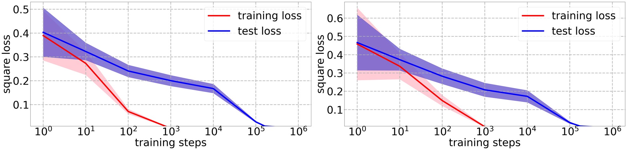
Figure 1: Comparing training and test squared losses using GD with weight decay over 50 independent runs (with independent datasets and student initializations). Left: training a ridge regression model to learn the zero teacher; Right: training a two-layer ReLU neural network (training both layers) to learn the zero teacher. We scale the x-axis logarithmically, which is commonly adopted for plotting the grokking phenomenon (Power et al., 2022; Lyu et al., 2024; Xu et al., 2024; Mohamadi et al., 2024). See Section 5 for further details of the experimental setup.
图 1:用带权衰减的 GD,在 50 次独立运行(数据集和学生初始化均独立)中比较训练平方损失与测试平方损失。左:训练岭回归模型以学习零教师;右:训练两层 ReLU 神经网络(两层都训)以学习零教师。横轴按对数尺度,这是绘制 grokking 现象时的常用做法(Power et al., 2022; Lyu et al., 2024; Xu et al., 2024; Mohamadi et al., 2024)。实验设置的更多细节见第 5 节。
In a bit more detail, our main contributions are as follows:
再稍作展开,我们的主要贡献如下:
- We study an over-parameterized ridge regression problem (Section 4), and show the first end-to-end provable grokking result (Theorem 4.2) for learning any realizable teacher function using gradient descent. Specifically, we prove the following separate components: – We prove that when optimizing the regularized squared loss using gradient descent, the training (empirical) squared error decays at a fast convergence rate (Theorem 4.4). – We provide a lower bound for the generalization error which admits a slower convergence rate than the one for the training error, implying long-term overfitting (Theorem 4.5). – Lastly, we show that gradient descent will eventually reach a global minimum with a generalization guarantee (Theorem 4.6).
- 我们研究过参数岭回归问题(第 4 节),并给出用梯度下降学习任意可实现教师函数时,第一组端到端可证明的 grokking 结果(定理 4.2)。具体来说,我们分别证明如下几个部分:– 我们证明,用梯度下降优化带 正则的平方损失时,训练(经验)平方误差以较快的速率衰减(定理 4.4)。– 我们为泛化误差给出一个下界,其收敛速率慢于训练误差,从而意味着长时间的过拟合(定理 4.5)。– 最后,我们证明梯度下降最终会到达具有泛化保证的全局最小值(定理 4.6)。
- We quantitatively state the sufficient conditions of the hyperparameters to realize grokking (Equations (3), (4) and (5)) and provide a rigorous lower bound on the grokking time in terms of model hyperparameters (Equations (6) and (7)). We then analyze how different hyperparameters affect grokking, which is in keeping with our experimental verifications.
- 我们定量给出实现 grokking 的超参数充分条件(式 (3)、(4) 和 (5)),并就 grokking 时间给出用模型超参数写出的严格下界(式 (6) 和 (7))。随后我们分析不同超参数如何影响 grokking,这与我们的实验验证相符。
- We support our theoretical findings with empirical simulations that illustrate how grokking can be controlled in a principled manner (Section 5).
- 我们用经验模拟支持理论结果,说明 grokking 可以按有原则的方式加以控制(第 5 节)。
- Finally, we conduct experiments on non-linear neural networks, and demonstrate empirically that the dependencies of the grokking time on hyperparameters qualitatively match our provable predictions in linear regression.
- 最后,我们在非线性神经网络上做实验,经验表明 grokking 时间对超参数的依赖,在定性上与我们在线性回归中可证明的预测相符。
1.1 Additional Related Work
1.1 其他相关工作
The intriguing phenomenon of grokking was first coined by Power et al. (2022), who observed it when training on algorithmic datasets for modular addition. However, the underlying behavior—where generalization emerges long after overfitting—had already been noted in earlier work by Blanc et al. (2020), in the context of matrix sensing and simplified shallow neural networks. Following these seminal works, grokking has also been observed in other learning paradigms, which include learning sparse parities (Barak et al., 2022; Merrill et al., 2023), learning the greatest common divisor of integers (Charton, 2024), and image classification (Radhakrishnan et al., 2022).
grokking 这一引人注目的现象首先由 Power et al. (2022) 命名,他们是在模加法一类算法数据集上训练时观察到的。不过,泛化在过拟合很久之后才出现这一底层行为,早已被 Blanc et al. (2020) 在矩阵感知和简化浅层神经网络的语境中指出。在这些开创性工作之后,grokking 也在其他学习范式中被观察到,包括学习稀疏奇偶(Barak et al., 2022; Merrill et al., 2023)、学习整数的最大公约数(Charton, 2024),以及图像分类(Radhakrishnan et al., 2022)。
Several works proposed thoughtful ideas to explain grokking, although none of them provided rigorous end-to-end grokking results. Liu et al. (2022) offered an explanation via the lens of representation learning. Thilak et al. (2022) attributed grokking to the use of adaptive optimizers—an optimization anomaly named the “Slingshot Mechanism” (cyclic phase transitions). Liu et al. (2023) identified a mismatch between training and test loss landscapes, which they called the “LU mechanism”, and used it to explain certain aspects of grokking. Nanda et al. (2023) revealed that grokking can arise from the gradual amplification of structured mechanisms encoded in the weights via progress measuring. Davies et al. (2023) hypothesized that grokking and double descent can be understood using the same pattern-learning model, and provided the first demonstration of model-wise grokking. Merrill et al. (2023) studied the problem of training two-layer neural networks on a sparse parity task, and attributed grokking therein to the competition between dense and sparse subnetworks. Gromov (2023) demonstrated that fully-connected two-layer networks exhibit grokking on modular arithmetic tasks without any regularization and attributed grokking to feature learning. Miller et al. (2024) studied grokking beyond neural networks, e.g. Bayesian models. Beck et al. (2025) explored the phenomenon of grokking in a logistic regression problem. They provided evidence that grokking may occur under some asymptotic assumptions on the hyperparameters, but they did not rigorously prove grokking. Varma et al. (2023) interpreted grokking from the perspective of circuit efficiency, and discovered two related phenomena named “ungrokking” and “semi-grokking”. Jeffares et al. (2024) provided empirical insights into grokking, by investigating a telescoping model that suggests that grokking may reflect a transition to a measurably benign overfitting regime during training. Humayun et al. (2024) attributed grokking of deep neural networks to their delayed robustness. Prieto et al. (2025) demonstrated the dependence of grokking on regularization by showing that Softmax Collapse (i.e. floating point errors due to numerical instability) is responsible for the absence of grokking without regularization. We note that in addition to Prieto et al. (2025), several other papers considered grokking without explicit regularization (e.g., Xu et al. (2024); Levi et al. (2024)), but the grokking literature mostly focuses on settings with explicit regularization, as in this paper. Mallinar et al. (2025) revealed that grokking is not specific to neural networks nor to GD-based optimization methods by showing that grokking occurs when learning modular arithmetic with Recursive Feature Machines (RFM). Žunkovič and Ilievski (2024) analyzed grokking in linear classification, and showed quantitative bounds on the grokking time, but they did not provide rigorous proofs. Yunis et al. (2024) showed empirically that grokking is connected to rank minimization, namely, that the sudden drop in the test loss coincides precisely with the onset of low-rank behavior in the singular values of the weight matrices. Jeffares and van der Schaar (2025) argue that the settings in which grokking and other counterintuitive phenomena in deep learning can be shown to occur are limited in practice, as they may only appear in very specific situations.
已有若干工作提出了有启发的想法来解释 grokking,但其中没有一项给出严格的端到端 grokking 结果。Liu et al. (2022) 从表示学习的角度给出解释。Thilak et al. (2022) 把 grokking 归因于自适应优化器的使用——一种称为「弹弓机制」(Slingshot Mechanism)的优化异常(循环相变)。Liu et al. (2023) 指出训练损失景观与测试损失景观之间存在错配,并称之为「LU 机制」,用它来解释 grokking 的某些方面。Nanda et al. (2023) 揭示,grokking 可以来自权重中所编码的结构化机制经由进度度量被逐步放大。Davies et al. (2023) 提出,grokking 与双重下降可以用同一套模式学习模型来理解,并首次展示了模型维(model-wise)grokking。Merrill et al. (2023) 研究在稀疏奇偶任务上训练两层神经网络,并把其中的 grokking 归因于稠密子网络与稀疏子网络之间的竞争。Gromov (2023) 表明,全连接两层网络在模运算任务上即使不加任何正则也会出现 grokking,并将其归因于特征学习。Miller et al. (2024) 研究了超出神经网络的 grokking,例如贝叶斯模型。Beck et al. (2025) 探索了逻辑回归中的 grokking。他们给出证据,表明在超参数的某些渐近假设下可能出现 grokking,但并没有严格证明 grokking。Varma et al. (2023) 从回路效率的角度解释 grokking,并发现了两个相关现象,分别称为「ungrokking」和「semi-grokking」。Jeffares et al. (2024) 通过考察一个套叠(telescoping)模型,为 grokking 提供了经验见解,该模型表明 grokking 可能反映训练过程中向可度量的良性过拟合区间的转变。Humayun et al. (2024) 把深度神经网络的 grokking 归因于其延迟稳健性。Prieto et al. (2025) 通过表明 Softmax 崩溃(Softmax Collapse,即数值不稳定带来的浮点误差)是没有正则时观察不到 grokking 的原因,展示了 grokking 对正则化的依赖。我们注意到,除了 Prieto et al. (2025) 之外,也有若干论文考虑了没有显式正则的 grokking(例如 Xu et al. (2024); Levi et al. (2024)),但 grokking 文献大多像本文一样,关注带显式正则的设定。Mallinar et al. (2025) 表明 grokking 并不专属于神经网络,也不专属于基于 GD 的优化方法:在用递归特征机(Recursive Feature Machines,RFM)学习模运算时也会出现 grokking。Žunkovič and Ilievski (2024) 分析了线性分类中的 grokking,并给出了 grokking 时间的定量界,但他们没有提供严格证明。Yunis et al. (2024) 从经验上表明 grokking 与秩最小化有关,也就是说,测试损失的突然下降恰好与权矩阵奇异值开始呈现低秩行为同时发生。Jeffares and van der Schaar (2025) 认为,能够展示 grokking 以及深度学习中其他反直觉现象的设定在实践中相当有限,因为它们可能只在非常特定的情形下出现。
1.2 Organization
1.2 文章结构
The remaining of the paper is organized as follows. In Section 2, we formally describe the problem setup and introduce necessary notations. In Section 3, we provide an informal theorem to convey our main results in an accessible manner. In Section 4, we present our main results of end-to-end provable grokking in ridge regression. In Section 5, we support our theory with empirical verifications. In Section 6, we conclude the paper and propose some interesting future research directions. All proofs and additional experiments are deferred to the appendix.
本文其余部分安排如下。第 2 节形式化描述问题设定并引入必要记号。第 3 节给出一个非正式定理,以便用更易读的方式呈现主要结果。第 4 节给出岭回归中端到端可证明 grokking 的主要结果。第 5 节用经验验证支持理论。第 6 节总结全文并提出若干有意思的未来研究方向。全部证明和补充实验放在附录中。
2 Preliminaries
2 预备知识
Notations. We use bold-face letters to denote vectors such as and use bold-face capital letters to denote matrices such as . We denote by the -dimensional identity matrix. For a vector , we denote by its norm. For a matrix , we denote by and its operator and Frobenius norms, respectively. For a symmetric matrix , let and denote its smallest eigenvalue and its smallest positive eigenvalue, respectively. We use to denote the indicator function, which equals one when its Boolean input is true and zero otherwise. We use standard asymptotic notations and to hide numerical constant factors.
记号。 我们用粗体小写字母表示向量,例如 ,用粗体大写字母表示矩阵,例如 。我们用 表示 维单位矩阵。对向量 ,用 表示其 范数。对矩阵 ,分别用 和 表示其算子范数和 Frobenius 范数。对对称矩阵 ,分别用 和 表示其最小特征值和最小正特征值。我们用 表示示性函数,当其布尔输入为真时取一,否则取零。我们使用标准的渐近记号 和 来隐去数值常数因子。
Linear regression and data generation. We consider a fundamental regression problem of learning a teacher function where . The training data are generated according to the following: the input follows some marginal distribution (which we do not specify), and is exactly labeled by the teacher function, i.e. . We train a student linear regression model
线性回归与数据生成。 我们考虑学习教师函数 这一基本回归问题,其中 。训练数据 按如下方式生成:输入 服从某个边际分布 (我们不对其作具体指定),并由教师函数精确标注,即 。我们训练一个学生线性回归模型
where is some fixed feature map and is the trainable parameters, to learn the teacher. We assume that the teacher is realizable, i.e., for some .
其中 是某个固定的特征映射, 是可训练参数,用来学习教师。我们假设教师是可实现的,即对某个 ,有 。
Ridge regression. In a regression problem, it is natural to train the model by minimizing the empirical mean squared loss and evaluate the learning performance on the population squared loss . We use ridge regression by appending an -regularization term to the loss function. Let denote the regularized mean squared training error, let denote the unregularized mean squared loss, and let denote the penalty. Our training objective is
岭回归。 在回归问题中,自然的做法是通过最小化经验均方损失 来训练模型,并在总体平方损失 上评估学习表现。我们使用岭回归,也就是在损失函数上附加一项 正则。设 表示正则化后的均方训练误差, 表示未正则化的均方损失, 表示 惩罚项。我们的训练目标是
where is the regularization parameter. We scale the loss objective by a constant factor of for the simplicity of gradient analysis. We optimize Equation (1) using the vanilla Gradient Descent (GD) algorithm, which updates via
其中 是正则化参数。为了简化梯度分析,我们把损失目标乘上常数因子 。我们用普通的梯度下降(GD)算法优化式 (1),它通过如下方式更新
where is the step-size or learning rate. While we focus on GD with a fixed step size, we note that our analysis should also hold for GD with a decaying step size and for gradient flow.
其中 是步长或学习率。尽管我们关注固定步长的 GD,但需要指出,我们的分析也应当适用于步长递减的 GD 以及梯度流。
When and , our loss objective in Equation (1) can be simplified to
当 且 时,式 (1) 中的损失目标可以简化为
and each GD iteration realizes an update in the form of
并且每一次 GD 迭代实现如下形式的更新
To present our results, we introduce the following additional notations. Let denote the generalization (population) squared loss. We define the empirical feature map as . Let denote the (average) norm of the feature vectors. Let denote the feature population covariance matrix.
为了陈述结果,我们再引入如下记号。设 表示泛化(总体)平方损失。我们把经验特征映射定义为 。设 表示特征向量的(平均)范数。设 表示特征的总体协方差矩阵。
3 Informal Results
3 非正式结果
To demonstrate a clear manifestation of grokking, our main theorem is formulated as follows: GD achieves a training error smaller than in an early stage of training (at step ), while a poor generalization error well above some constant persists far beyond the point of overfitting (until step ), yet eventually a generalization error smaller than is reached. In particular, this establishes grokking when . Our results give a lower bound on in terms of both and , where this difference can be made arbitrarily large via proper hyperparameter tuning for any choice of and . Specifically, let be the largest number of training steps such that the empirical squared loss is above , and let be the smallest number of training steps for which the generalization loss is below . Our main results are summarized by the following informal theorem, establishing end-to-end provable grokking in ridge regression.
为了把 grokking 表现得足够清楚,我们把主要定理表述如下:GD 在训练较早阶段(第 步)就把训练误差降到小于 ,而明显高于某个常数 的很差泛化误差会持续到过拟合点之后很久(直到第 步),但最终泛化误差仍会降到小于 。特别地,当 时,这就确立了 grokking。我们的结果给出 关于 和 的下界,并且对任意选定的 和 ,都可以通过适当的超参数调节把这一差值拉到任意大。具体来说,设 是经验平方损失仍高于 的最大训练步数,设 是泛化损失低于 的最小训练步数。下述非正式定理概括了我们的主要结果,确立了岭回归中端到端可证明的 grokking。
Informal Theorem(End-to-end provable grokking for ridge regression).
非正式定理(岭回归的端到端可证明 grokking)。
Consider a linear regression problem of training a student model to learn a realizable teacher $N^{}(\bm{x})=\langle\bm{\theta}^{},\bm{\phi}(\bm{x})\rangle\bm{\theta}\in\mathbb{R}^{m}\bm{\theta}^{}n\bm{\theta}^{(0)}\lambda$.*
考虑如下线性回归问题:训练学生模型 ,以学习可实现教师 $N^{}(\bm{x})=\langle\bm{\theta}^{},\bm{\phi}(\bm{x})\rangle\bm{\theta}\in\mathbb{R}^{m}\bm{\theta}^{}n\bm{\theta}^{(0)}\lambda$ 的梯度下降。*
Under the initialization for some , and some mild distributional assumptions on the feature map , we have with high probability that for a sufficiently large sample size , and a sufficiently large feature space dimensionality , can be lower bounded by an arbitrarily large value by choosing a sufficiently small weight decay .
在初始化 (对某个 )以及特征映射 满足若干温和分布假设的条件下,我们以高概率得到:当样本量 足够大、特征空间维数 足够大时,只要把权衰减 取得足够小, 就可以被下界成任意大。
4 Grokking in Ridge Regression
4 岭回归中的 Grokking
We now formalize our end-to-end provable grokking results for ridge regression problems. For any realizable teacher function, we provide a quantitative lower bound for the grokking time in terms of training hyperparameters, as well as bounds on the hyperparameters that suffice to realize grokking. Based on these bounds, we analyze how the different hyperparameters affect grokking, which is corroborated in our experiments in Section 5.
我们现在把岭回归问题中端到端可证明的 grokking 结果形式化。对任意可实现的教师函数,我们用训练超参数给出 grokking 时间 的定量下界,以及足以实现 grokking 的超参数界。基于这些界,我们分析不同超参数如何影响 grokking,这与第 5 节的实验相一致。
4.1 Warmup: Grokking with the Zero Teacher
4.1 热身:零教师情形下的 Grokking
We start by considering a simple scenario where the target teacher is the zero function. When , we have
我们先考虑目标教师为零函数的简单情形。当 时,我们有
The following theorem describes an end-to-end provable grokking result for learning the zero teacher in a ridge regression setting using gradient descent. To develop some initial intuition on what causes grokking, we state the aforementioned three stages of grokking in terms of the convergence rates of the training/generalization squared losses, in contrast to the format of our Theorem 4.2 which appears later.
下述定理给出在岭回归设定下用梯度下降学习零教师时,端到端可证明的 grokking 结果。为了对 grokking 的成因建立初步直觉,我们用训练/泛化平方损失的收敛速率来陈述前述三个 grokking 阶段,这与稍后出现的定理 4.2 的表述形式不同。
Theorem 4.1(End-to-end provable grokking for the zero teacher).
定理 4.1(零教师情形的端到端可证明 grokking)。
Suppose that the teacher function is $N^{}(\bm{x})=0N(\bm{x};\bm{\theta})=\langle\bm{\theta},\bm{\phi}(\bm{x})\rangle\bm{\theta}^{(0)}\sim\mathcal{N}(\bm{0},\nu^{2}\bm{I}_{m})\eta\leq 2/(L+2\lambda)t\in\mathbb{N}$, we have*
设教师函数为 $N^{}(\bm{x})=0N(\bm{x};\bm{\theta})=\langle\bm{\theta},\bm{\phi}(\bm{x})\rangle\bm{\theta}^{(0)}\sim\mathcal{N}(\bm{0},\nu^{2}\bm{I}_{m})\eta\leq 2/(L+2\lambda)t\in\mathbb{N}$,我们有*
- With probability at least,
- 以至少 的概率,
Studying the zero teacher as a warmup yields the following advantages. First, choosing the zero teacher enables us to build a much simpler generalization guarantee. Clearly, item (iii) above implies that GD eventually converges to the solution . Since , this yields generalization. Additionally, choosing the zero teacher allows us to derive matching lower (ii) and upper (iii) bounds for the generalization loss in terms of the convergence rate.
把零教师作为热身来研究,有如下好处。首先,选择零教师使我们能够建立简单得多的泛化保证。显然,上面的第 (iii) 项意味着 GD 最终会收敛到解 。由于 ,这就给出了泛化。此外,选择零教师还使我们能够就泛化损失给出在收敛速率上相匹配的下界 (ii) 与上界 (iii)。
More importantly, Theorem 4.1 reveals that the training and test losses can decrease at different rates, and the potentially considerable discrepancy between these rates causes grokking. Specifically, given the empirical feature map , a sufficiently small regularization can only have a negligible effect on the convergence rate of the training MSE. This is because the convergence rate of will be dominated by the term when is sufficiently small. However, decreasing can make the generalization convergence rate arbitrarily slow. In conclusion, Theorem 4.1 establishes a provable instance of grokking whenever , and .
更重要的是,定理 4.1 揭示出训练损失和测试损失可以按不同速率下降,而这两种速率之间可能相当可观的差距,正是 grokking 的成因。具体来说,给定经验特征矩阵 ,足够小的正则 对训练 MSE 的收敛速率几乎没有影响。这是因为当 足够小时, 的收敛速率将被 主导。但是,减小 却可以使泛化收敛速率 变得任意慢。总之,只要 、 且 ,定理 4.1 就给出了一个可证明的 grokking 实例。
4.2 Grokking with Realizable Teachers
4.2 可实现教师情形下的 Grokking
For the most general setting studied in this paper, we consider the realizable case where the ground-truth teacher is for some unknown , and the student is where is the vector of trainable parameters. We show that for any teacher, there is a realization of training hyperparameters that results in an arbitrarily long grokking time. Our main result is the following.
就本文研究的最一般设定而言,我们考虑可实现情形:真实教师为 ,其中 未知;学生为 ,其中 是可训练参数向量。我们证明,对任意教师,都存在一组训练超参数的实现,使得 grokking 时间可以任意长。我们的主要结果如下。
Theorem 4.2(End-to-end provable grokking for realizable ridge regression).
定理 4.2(可实现岭回归的端到端可证明 grokking)。
Assume a realizable teacher function $N^{}(\bm{x})=\langle\bm{\theta}^{},\bm{\phi}(\bm{x})\rangle\bm{\theta}^{}\in\mathbb{R}^{m}\lVert\bm{\phi}(\bm{x})\rVert_{2}\leq b\bm{x}b>0N(\bm{x};\bm{\theta})=\langle\bm{\theta},\bm{\phi}(\bm{x})\rangle\bm{\theta}^{(0)}\sim\mathcal{N}(\bm{0},\nu^{2}\bm{I}_{m})\epsilon>0c\geq\epsilon$ be arbitrary. We define*
假设存在可实现的教师函数 $N^{}(\bm{x})=\langle\bm{\theta}^{},\bm{\phi}(\bm{x})\rangle\bm{\theta}^{}\in\mathbb{R}^{m}\bm{x}b>0\lVert\bm{\phi}(\bm{x})\rVert_{2}\leq bN(\bm{x};\bm{\theta})=\langle\bm{\theta},\bm{\phi}(\bm{x})\rangle\bm{\theta}^{(0)}\sim\mathcal{N}(\bm{0},\nu^{2}\bm{I}_{m})\epsilon>0c\geq\epsilon$ 为任意常数。我们定义*
and
以及
For any , assume a sufficiently large sample size:
对任意 ,假设样本量足够大:
a sufficiently large dimensionality of the feature map:
特征映射的维数足够大:
and finally, a sufficiently small weight decay:
最后,权衰减足够小:
Then, if , we have with probability at least that
那么,若 ,则以至少 的概率,我们有
and
以及
Moreover, for all sufficiently large .
此外,对所有足够大的 ,有 。
The main intuition behind this discrepancy between and can be explained as follows: When the student regression model is sufficiently over-parameterized (), we are solving a high-dimensional regression problem. Therefore, when the weight decay is small, the GD optimization process only effectively updates the projection of the weight vector onto the data-spanning subspace to fit the training data, while having negligible effect on the component in the complementary subspace, which remains close to its initialization. This occurs since the information captured by the data only contributes to the convergence of at a rate of . In contrast, converges at a negligible rate of as a consequence of long-term weight decay. Such an imbalanced trajectory prevents timely generalization and leads to harmful overfitting. As a remedy, weight decay plays a crucial role in decreasing the complexity of the model class, which eventually guarantees uniform convergence and thus good generalization.
关于 与 之间这一差距的主要直觉,可以解释如下:当学生回归模型充分过参数化()时,我们是在解一个高维回归问题。因此,当权衰减 较小时,GD 优化过程只会有效更新权向量在数据张成子空间上的投影 ,以拟合训练数据,而对互补子空间中的分量 几乎没有影响,后者仍接近其初始化。之所以如此,是因为数据所捕获的信息只以 的速率贡献于 的收敛。与此相对, 以可忽略的速率 收敛,这是长期权衰减的结果。这样不平衡的轨迹妨碍了及时泛化,并导致有害的过拟合。作为补救,权衰减在降低模型类复杂度方面起着关键作用,最终保证一致收敛,从而保证良好的泛化。
Next, we disentangle the influence of individual hyperparameters on the grokking time according to our theory, which aligns closely with our experimental results in Section 5. Notably, these functional dependencies on the hyperparameters are not only qualitatively corroborated by our experiments, but they also quantitatively predict the expected scaling rates (see Figure 2).
接下来,我们按理论把各个超参数对 grokking 时间的影响拆开,这与第 5 节的实验结果密切相符。值得注意的是,这些关于超参数的函数依赖不仅在定性上得到实验支持,而且在定量上也能预测期望的缩放速率(见图 2)。
Evidently, Equations (6) and (7) together provide strong control of the grokking time , which reveals the following effects of hyperparameter tuning on grokking:
显然,式 (6) 和式 (7) 合在一起对 grokking 时间 给出了很强的控制,并从中可以看出超参数调节对 grokking 的如下影响:
- Weight decay : For small , decreasing increases with when other hyperparameters are held fixed, and has no effect on our bound for . Therefore, as . We remark that for large (which is not our focus in this work), our upper bound in Equation (6) is not tight in general, as a tight bound should incorporate the term in the denominator.
- 权衰减 :当 较小时,在其他超参数固定的前提下,减小 会使 增大,并且 ,而 对我们给出的 的界没有影响。因此,当 时,。需要说明的是,对较大的 (这不是本文的重点),式 (6) 中的上界一般并不紧,因为紧的界应当在分母中纳入 这一项。
- Sample size and feature dimensionality : It is difficult to deduce clean dependencies that capture the behavior of as a function of and , since there is no known quantitative bound revealing how depends on and , even when making strong assumptions on the distribution of the features (see Remark 4.3 for a discussion). On a more positive note, we show empirically that the behavior of as a function of and strongly accords with our theoretical bound in Equation (6). As for , since we make no assumption on the feature map , the quantity is not necessarily controlled. Indeed, more explicit dependencies of on and can be derived by assuming distributional assumptions. For instance, if are i.i.d. spherical Gaussian vectors. We present such clean bounds in Equation (8) and show that it strongly matches our experimental results.
- 样本量 与特征维数 :要推出能够刻画 作为 和 的函数行为的干净依赖关系并不容易,因为即便对特征分布作很强的假设,目前也还没有定量界揭示 如何依赖于 和 (讨论见备注 4.3)。较为正面的是,我们从经验上表明, 作为 和 的函数,其行为与式 (6) 中的理论界高度一致。至于 ,由于我们对特征映射 不作假设,量 不一定能被控制。确实,若再加入分布假设,就可以推出 对 和 更显式的依赖。例如,设 是独立同分布的球面高斯向量。我们在式 (8) 中给出这样干净的界,并表明它与实验结果高度吻合。
- Initialization scale : Increasing increases and simultaneously with . More precisely, when is sufficiently small, we have , and moreover and for some and some . In such a scenario, increasing increases and amplifies grokking.
- 初始化尺度 :增大 会同时增大 和 ,并且 。更精确地说,当 足够小时,有 ,并且存在某些 以及某些 ,使得 且 。在这种情形下,增大 会增大 ,从而放大 grokking。
Remark 4.3(on and its dependence on and ).
备注 4.3(关于 及其对 和 的依赖)。
is an empirical quantity which depends on the sampled features. We note that even for simple distributions such as , the behavior of as a function of and is not yet fully understood. While there is a known asymptotic result given by the celebrated Marchenko–Pastur law (Marčenko and Pastur, 1967), showing that when and for some , , to the best of our knowledge, there is no quantitative bound revealing how this depends on and .
是依赖于所采样特征的经验量。我们注意到,即便对 这样简单的分布, 作为 和 的函数,其行为也尚未被完全理解。虽然著名的 Marchenko–Pastur 定律(Marčenko and Pastur, 1967)给出了已知的渐近结果:当 且 (对某个 )时,,但据我们所知,还没有定量界揭示它如何依赖于 和 。
Next, we state a separate theorem for each of the three stages of our grokking result, as it is helpful for understanding each hyperparameter effect separately.
接下来,我们为 grokking 结果的三个阶段分别陈述一条定理,这有助于分别理解各个超参数的影响。
Theorem 4.4(Training loss convergence).
定理 4.4(训练损失的收敛)。
Suppose that $N^{}(\bm{x})=\langle\bm{\theta}^{},\bm{\phi}(\bm{x})\rangle\bm{\theta}^{}\in\mathbb{R}^{m}\bm{\theta}^{(0)}\sim\mathcal{N}(\bm{0},\nu^{2}\bm{I}_{m})\eta<1/(\lambda+\lambda_{\mathrm{max}}(\bm{\Phi}^{\top}\bm{\Phi})/n)\epsilon>0\delta\in(0,1)$, suppose that*
设 $N^{}(\bm{x})=\langle\bm{\theta}^{},\bm{\phi}(\bm{x})\rangle\bm{\theta}^{}\in\mathbb{R}^{m}\bm{\theta}^{(0)}\sim\mathcal{N}(\bm{0},\nu^{2}\bm{I}_{m})\eta<1/(\lambda+\lambda_{\mathrm{max}}(\bm{\Phi}^{\top}\bm{\Phi})/n)\epsilon>0\delta\in(0,1)$,设*
and
以及
Then, with probability at least , we have for all
那么,以至少 的概率,对所有满足下式的 ,有
The above assumption that implies that the student is initialized to have a large norm with respect to the teacher’s norm. Since we aim to upper bound and not , the assumed upper bound on is for technical purposes, and it does not limit our results since small values of facilitate grokking.
上面关于 的假设意味着,学生被初始化成相对于教师范数而言具有较大范数。由于我们要上界的是 而不是 ,对 所假设的上界是出于技术原因;它并不限制我们的结果,因为较小的 反而有助于 grokking。
Theorem 4.5(Poor generalization when overfitting).
定理 4.5(过拟合时的较差泛化)。
Suppose that $N^{}(\bm{x})=\langle\bm{\theta}^{},\bm{\phi}(\bm{x})\rangle\bm{\theta}^{}\in\mathbb{R}^{m}\bm{\theta}^{(0)}\sim\mathcal{N}(\bm{0},\nu^{2}\bm{I}_{m})\eta<1/\lambdac>0\delta\in(0,1)$, suppose that*
设 $N^{}(\bm{x})=\langle\bm{\theta}^{},\bm{\phi}(\bm{x})\rangle\bm{\theta}^{}\in\mathbb{R}^{m}\bm{\theta}^{(0)}\sim\mathcal{N}(\bm{0},\nu^{2}\bm{I}_{m})\eta<1/\lambdac>0\delta\in(0,1)$,设*
Then, with probability at least , we have for all
那么,以至少 的概率,对所有满足下式的 ,有
The lower bound on here is stronger than the one in Theorem 4.4, which ensures that we are in a high-dimensional regression situation. In our last theorem, we prove that good generalization eventually occurs.
这里对 的下界比定理 4.4 中的更强,这保证我们处于高维回归情形。在最后一条定理中,我们证明良好的泛化最终会发生。
Theorem 4.6(Generalization).
定理 4.6(泛化)。
Suppose that $N^{}(\bm{x})=\langle\bm{\theta}^{},\bm{\phi}(\bm{x})\rangle\bm{\theta}^{}\in\mathbb{R}^{m}\lVert\bm{\phi}(\bm{x})\rVert_{2}\leq b\bm{x}b>0\bm{\theta}^{}{\lambda}=\argmin{\bm{\theta}}\left{L_{n}(\bm{\theta};\lambda)\right}\epsilon>0\delta\in(0,1)$, suppose that
设 $N^{}(\bm{x})=\langle\bm{\theta}^{},\bm{\phi}(\bm{x})\rangle\bm{\theta}^{}\in\mathbb{R}^{m}\bm{x}b>0\lVert\bm{\phi}(\bm{x})\rVert_{2}\leq b\bm{\theta}^{}{\lambda}=\argmin{\bm{\theta}}\left{L_{n}(\bm{\theta};\lambda)\right}\epsilon>0\delta\in(0,1)$,设
Then, if , GD converges to $\bm{\theta}^{}{\lambda}L(\bm{\theta}^{*}{\lambda})\leq 2L_{n}(\bm{\theta}^{}_{\lambda})+\epsilon1-\delta$.
那么,若 ,则 GD 收敛到满足 $L(\bm{\theta}^{}{\lambda})\leq 2L{n}(\bm{\theta}^{}_{\lambda})+\epsilon\bm{\theta}^{}_{\lambda}1-\delta$。*
The lower bound on the sample size stems from a standard uniform convergence argument based on Rademacher complexity.
对样本量的下界 来自基于 Rademacher 复杂度的标准一致收敛论证。
5 Experiments
5 实验
In this section, we systematically verify our theoretical understanding of grokking via experiments. Throughout, we use and to denote the training sample size, GD step size and weight decay parameter, respectively. In all of our experiments, we set the error thresholds .
本节我们通过实验系统验证对 grokking 的理论理解。全文用 、 和 分别表示训练样本量、GD 步长和权衰减参数。在所有实验中,我们把误差阈值都设成 。
5.1 Hyperparameter Control
5.1 超参数控制
We empirically verify our quantitative bounds on how the model’s hyperparameters affect grokking in realizable ridge regression. Specifically, we train a student linear regression model using gradient descent with weight decay, to learn a realizable teacher with unit norm, i.e. . We simply choose the feature map to be the identity function, i.e. . We use to denote the initialization scale of weights in line with our theory.
我们从经验上验证,在可实现岭回归中,模型超参数如何影响 grokking 的定量界。具体来说,我们用带权衰减的梯度下降训练学生线性回归模型,以学习范数为 1 的可实现教师,即 。我们简单地取特征映射为恒等函数,即 。与理论保持一致,我们用 表示权重的初始化尺度。
As discussed in Section 4, cannot be controlled without making additional assumptions on . Consequentially, by introducing additional distributional assumptions, we are able to provide more explicit bounds for and based on Theorem 4.2. Specifically, we assume that are drawn i.i.d. from a Gaussian distribution . In such a case, if , a simple calculation (see Remark A.14 for details) yields that
如第 4 节所讨论,若不对 作额外假设, 便无法被控制。因此,引入额外的分布假设后,我们就能基于定理 4.2 为 和 给出更显式的界。具体来说,我们假设 独立同分布地取自高斯分布 。在这种情形下,若 ,简单计算(细节见备注 A.14)可得
Our experiments are also implemented with such a distributional assumption. We set , and unless otherwise stated for comparison purposes, we use the default values , , and .
我们的实验也是在这样的分布假设下实现的。我们取 ,并且除非另有说明以便比较,默认取 、、 和 。
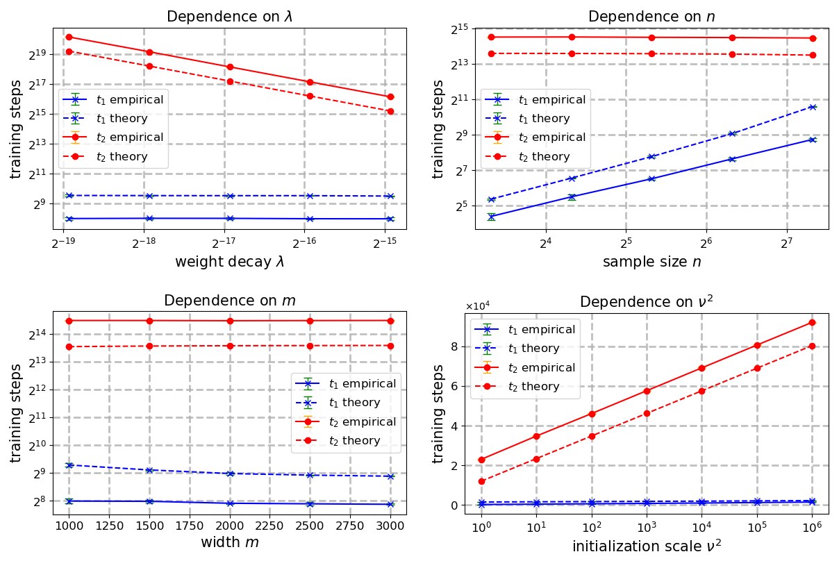
Figure 2: Plots for the effects of hyperparameters on grokking in ridge regression. Left Upper: decreasing weight decay extends the generalization delay (); Right Upper: decreasing sample size amplifies grokking by speeding up the convergence of the training loss (affects ); Left Lower: increasing the feature dimension has little effect on and ; Right Lower: increasing the initialization scale increases and simultaneously at logarithmic rates ().
图 2:岭回归中超参数对 grokking 影响的曲线。左上:减小权衰减会延长泛化延迟();右上:减小样本量会加快训练损失的收敛(影响 ),从而放大 grokking;左下:加大特征维对 和 几乎没有影响;右下:加大初始化尺度会同时按对数速率增大 和 ()。
The results are shown in Figure 2, where the dashed lines represent our theoretical bounds for and in Equation (8), and solid lines represent the values of and that were observed empirically. Notably, all pairs of solid and dashed lines seem to match in their behavior, implying that our theoretical bounds provide strong control.
结果见图 2,其中虚线表示式 (8) 中我们对 和 的理论界,实线表示经验观察到的 和 取值。值得注意的是,每一对实线与虚线在走势上都显得吻合,说明我们的理论界提供了很强的控制。
5.2 Random-Features Neural Networks
5.2 随机特征神经网络
In this subsection, we train a two-layer random ReLU features network to learn a single ReLU neuron teacher network with unit norm weights, i.e. with , where is the ReLU activation. A two-layer ReLU neural network is in the form of for all . For random-features neural networks, we only optimize the output layer weights , and the hidden layer weights are initialized and then fixed during training. Clearly, this random feature model is a special case of linear regression with feature map where for all . We use the following initialization scheme for each .
本小节中,我们训练一个两层随机 ReLU 特征网络,以学习权重范数为 1 的单 ReLU 神经元教师网络,即 且 ,其中 是 ReLU 激活。两层 ReLU 神经网络的形式为:对所有 ,。对随机特征神经网络,我们只优化输出层权重 ,隐层权重在初始化后于训练中保持固定。显然,这一随机特征模型是线性回归的特例,特征映射为 ,其中对所有 有 。我们采用如下初始化方案:对每个 ,,。
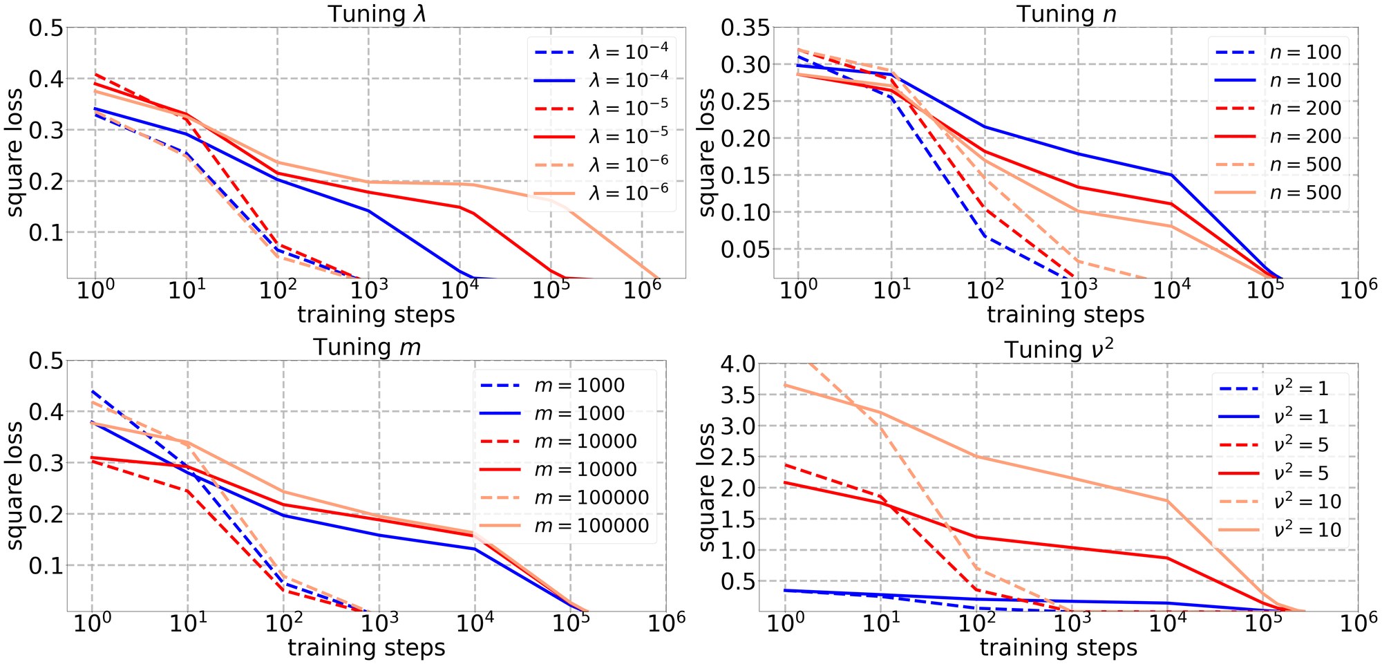
Figure 3: Plots of training and test losses of a two-layer random ReLU features network. Dashed/solid lines indicate train/test loss respectively. Left Upper: using smaller weight decay amplifies the grokking time by delaying generalization (increases ); Right Upper: having smaller sample size amplifies grokking by speeding up the training convergence (decreases ); Left Lower: increasing the student’s width does not significantly prolong grokking; Left Lower: increasing the initialization scale does not significantly prolong grokking, but instead widens the gap between the generalization and training losses during the overfitting stage.
图 3:两层随机 ReLU 特征网络的训练损失与测试损失曲线。虚线/实线分别表示训练/测试损失。左上:使用更小的权衰减会推迟泛化(增大 ),从而放大 grokking 时间;右上:更小的样本量会加快训练收敛(减小 ),从而放大 grokking;左下:加大学生宽度并不会显著延长 grokking;右下:加大初始化尺度并不会显著延长 grokking,但会在过拟合阶段拉大泛化损失与训练损失之间的差距。
We present the results in Figure 3, by a standard comparison between the training and test losses. We set: , , and unless otherwise stated for comparison purposes, we use the default values , , and . Since the teacher is sampled independently of the student network, this sets us in a non-realizable setting. However, since a sufficiently wide student network can approximate any teacher to arbitrary accuracy with high probability, we are essentially arbitrarily close to the realizable setting with sufficient over-parameterization. The figure shows behavior similar to that of realizable ridge regression.
我们在图 3 中以训练损失与测试损失的标准比较来呈现结果。我们取:,,并且除非另有说明以便比较,默认取 、、 和 。由于教师 是独立于学生网络采样的,这把我们放在了不可实现的设定中。不过,足够宽的学生网络可以以高概率把任意教师逼近到任意精度,因此在充分过参数化时,我们实质上任意接近可实现设定。该图显示的行为与可实现岭回归相似。
5.3 Non-linear Neural Networks
5.3 非线性神经网络
We also study empirically the effects of the different hyperparameters on grokking for training (both layers of) a two-layer ReLU neural network as defined in Subsection 5.2 with . We use the following initialization scheme for each . Specifically, we choose the zero function to be the underlying teacher, and set , , and unless otherwise stated for comparison purposes, we use the default values , , and .
我们还从经验上研究,在训练(两层都训)第 5.2 小节所定义、参数为 的两层 ReLU 神经网络时,不同超参数对 grokking 的影响。我们采用如下初始化方案:对每个 ,,。具体来说,我们取零函数作为底层教师,并取 、,并且除非另有说明以便比较,默认取 、、 和 。
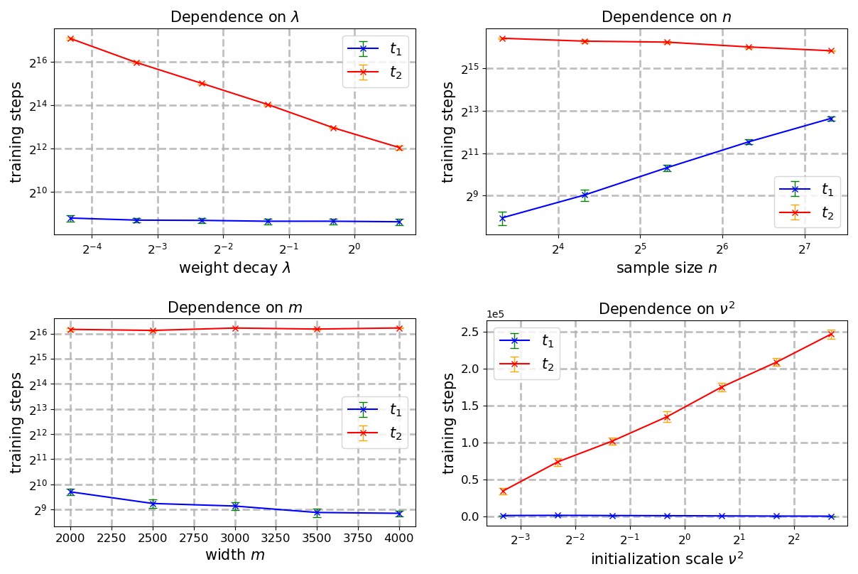
Figure 4: Plots for the effect of the hyperparameters on grokking when training a two-layer ReLU network with the zero teacher.
图 4:以零教师训练两层 ReLU 网络时,超参数对 grokking 的影响曲线。
The results are presented in Figure 4. Notably, the dependencies of and on the hyperparameters match qualitatively to those in Figure 2. This suggests that our bounds might capture behaviors that hold much more generally than our currently analyzed setting, and thus exploring it further is an intriguing direction for future work.
结果见图 4。值得注意的是, 和 对超参数的依赖在定性上与图 2 相符。这表明,我们的界所捕获的行为,其适用范围可能远大于当前已分析的设定,因此进一步探索是一个有吸引力的未来方向。
Finally, we include the experimental setup for Figure 1 for completeness. Left: , , , and ; Right: , , , , and . See Appendix B for additional experiments.
最后,为完整起见,我们补充图 1 的实验设置。左:,,, 且 ;右:,,,, 且 。补充实验见附录 B。
6 Discussion and Future Directions
6 讨论与未来方向
We study grokking and establish the first end-to-end provable grokking result for the classical ridge regression model. We derive quantitative bounds for the grokking time in terms of the model hyperparameters and verify our theoretical findings via experiments. Our work establishes a rigorous theoretical foundation for grokking. Observing this phenomenon within the fundamental framework of linear regression is not only surprising in its simplicity, but also highly illuminating; it provides a controlled environment that allows us to cleanly isolate the precise effects of individual hyperparameters. By uncovering the root causes of grokking in this transparent setting, our analysis may serve as a stepping stone toward demystifying its dynamics in modern deep learning architectures.
我们研究 grokking,并在经典岭回归模型上给出第一组端到端可证明的 grokking 结果。我们用模型超参数写出 grokking 时间的定量界,并用实验验证理论发现。这项工作为 grokking 建立了严格的理论基础。在线性回归这一基本框架里观察到这一现象,不仅因其简单而令人意外,也极具启发性:它提供了一个可控的环境,使我们能够干净地分离各个超参数的精确影响。通过在这一透明设定中揭示 grokking 的根源,我们的分析也许可以成为理解它在现代深度学习结构中动力学的一块垫脚石。
Our work leaves several interesting questions open. Firstly, can we show end-to-end provable grokking results for non-realizable ridge regression? This includes the special case of ridge regression with label noise (see Figure 6 in Appendix B). Since we have already observed grokking empirically in non-realizable learning with two-layer random-features neural networks, it is natural to start studying such random features models. Indeed, deriving provable grokking results for learning agnostically with two-layer ReLU random features neural networks seems challenging. We find that current theoretical analyses fail to identify a hyperparameter realization for grokking. Specifically, when using our techniques, choosing an arbitrarily small weight decay parameter in the agnostic learning setting may impede generalization entirely. This suggests that new tools and more careful convergence analyses might be required.
我们的工作留下了若干有意思的未解问题。首先,能否为不可实现的岭回归给出端到端可证明的 grokking 结果?这包括带标签噪声的岭回归这一特例(见附录 B 中的图 6)。既然我们已经在两层随机特征神经网络的不可实现学习中从经验上观察到 grokking,自然可以从这类随机特征模型入手。确实,要为用两层 ReLU 随机特征神经网络做不可知学习给出可证明的 grokking 结果,看起来相当困难。我们发现,现有理论分析无法为 grokking 找出一组超参数实现。具体来说,若沿用我们的技术,在不可知学习设定下把权衰减取得任意小,甚至可能彻底妨碍泛化。这说明可能需要新的工具和更细致的收敛分析。
Another question left open by our research is whether we can show end-to-end provable grokking as a result of a transition from the lazy to the rich regime of training neural networks. As discussed earlier, many existing works attribute grokking to such lazy-to-rich regime transitions, and have verified it empirically, but none provided a rigorous theoretical analysis proving it. Motivated by this, we have also explored grokking in a setting where we learn a target neural network teacher, by training a two-layer student network using GD with weight decay. Unlike the ridge regression setting addressed in this paper, proving that overfitting occurs remains challenging even under strong assumptions, such as a zero-teacher model where GD only optimizes the hidden layer weights. While a classical neural tangent kernel (NTK) analysis implies that each neuron remains close to its initialization during training, this does not guarantee persistent poor generalization; the collective contribution of neurons may still allow the trained network to converge toward the zero function.
我们的研究留下的另一个问题是:能否证明,作为神经网络训练从懒惰区走到富裕区的结果,也会出现端到端可证明的 grokking。如前所述,许多已有工作把 grokking 归因于这种从懒惰区到富裕区的转变,并在经验上予以验证,但没有一项给出证明这一点的严格理论分析。受此启发,我们也探索了如下设定中的 grokking:通过用带权衰减的 GD 训练两层学生网络,来学习一个目标神经网络教师。与本文处理的岭回归设定不同,即便在很强的假设下——例如零教师模型、且 GD 只优化隐层权重——要证明过拟合会发生仍然很困难。虽然经典的神经正切核(NTK)分析意味着每个神经元在训练中都保持接近其初始化,但这并不保证持续较差的泛化; 个神经元的集体贡献仍可能使训练后的网络向零函数收敛。
We note that when training with a small weight decay coefficient, the overfitting solution that we obtain corresponds to training without weight decay, and the asymptotic solution is the minimum-norm interpolating predictor, which corresponds to training with zero initialization without weight decay (Gunasekar et al., 2018; Vardi and Shamir, 2021). Hence, in our setting grokking corresponds to a transition from a misspecified to a well-specified prior. Moreover, Lauditi et al. (2025) showed that weight decay in wide non-linear neural networks may cause the initial NTK to decay leaving only a data-dependent NTK. Thus, similarly to our work, in their setting weight decay changes an implicit prior. However, it is unclear whether their prior change can lead to grokking.
我们注意到,当用较小的权衰减系数训练时,我们所得到的过拟合解对应于不带权衰减的训练,而渐近解是最小范数插值预测器,它对应于零初始化且不带权衰减的训练(Gunasekar et al., 2018; Vardi and Shamir, 2021)。因此,在我们的设定中,grokking 对应于从错误指定先验走到正确指定先验的转变。此外,Lauditi et al. (2025) 表明,宽的非线性神经网络中的权衰减可能使初始 NTK 衰减,只留下依赖于数据的 NTK。因此,与我们的工作类似,在他们的设定中权衰减也改变了隐式先验。不过,他们的先验改变是否会导致 grokking,目前并不清楚。
Finally, it is worth noting that grokking in regression tasks exhibits structural differences from its classification counterpart, particularly regarding the characteristic “test error plateau”. In classification, this plateau is typically an artifact of evaluating a discrete metric (accuracy) rather than a continuous loss (e.g. Gromov, 2023, Figure 1). In regression, however, the continuous loss is the natural primary metric, which typically decays smoothly without an explicit plateau. To bridge this gap and investigate whether our setting captures this classic phenomenon, we define a threshold-based surrogate accuracy metric given by for a fixed . Remarkably, evaluating our model under this metric reveals the familiar plateauing phenomenon experimentally (see Figure 5 in Appendix B). This confirms that the plateau is not unique to classification settings but can be recovered in linear regression under appropriate evaluation, offering a promising direction for future theoretical analysis.
最后值得指出的是,回归任务中的 grokking 与其分类对应物在结构上有所不同,尤其是在典型的「测试误差平台」方面。在分类中,这一平台通常是评估离散指标(精度)而非连续损失的产物(例如 Gromov, 2023, 图 1)。而在回归中,连续损失本身就是自然的主要指标,它通常会平滑下降,并没有显式的平台。为了弥合这一差距,并考察我们的设定是否捕获了这一经典现象,我们定义一个基于阈值的替代精度指标:,其中 固定。值得注意的是,用这一指标评估我们的模型,会在实验中显现出熟悉的平台现象(见附录 B 中的图 5)。这证实平台并不为分类设定所独有,在适当的评估方式下也可以在线性回归中被恢复,从而为未来的理论分析提供了一个有希望的方向。
Acknowledgements
致谢
We thank the anonymous reviewers who provided useful suggestions to improve the quality of this paper. GV is supported by the Israel Science Foundation (grant No. 2574/25), by a research grant from Mortimer Zuckerman (the Zuckerman STEM Leadership Program), and by research grants from the Center for New Scientists at the Weizmann Institute of Science, and the Shimon and Golde Picker – Weizmann Annual Grant. IS is supported by the Israel Science Foundation (grant No. 1753/25).
我们感谢匿名审稿人提出的有益建议,这些建议帮助提高了本文的质量。GV 得到以色列科学基金会(Israel Science Foundation,资助号 2574/25)、Mortimer Zuckerman 的研究资助(Zuckerman STEM Leadership Program),以及魏茨曼科学研究院新科学家中心(Center for New Scientists)和 Shimon and Golde Picker – Weizmann 年度资助的研究经费支持。IS 得到以色列科学基金会(资助号 1753/25)的支持。
Impact Statement
影响声明
This paper presents work whose goal is to advance the field of Machine Learning. Since this work is mainly theoretical in its nature, there are no societal implications that require discloser as far as we can discern.
本文工作的目标是推动机器学习领域的进展。由于这项工作在性质上主要是理论的,就我们所能分辨的范围而言,并不存在需要披露的社会影响。
References
参考文献
Barak et al. (2022) B. Barak, B. Edelman, S. Goel, S. Kakade, E. Malach, and C. Zhang Hidden progress in deep learning: sgd learns parities near the computational limit . Advances in Neural Information Processing Systems 35 , pp. 21750–21764 . Cited by: §1.1 .
Bartlett and Mendelson (2002) P. L. Bartlett and S. Mendelson Rademacher and gaussian complexities: risk bounds and structural results . Journal of Machine Learning Research 3 ( Nov ), pp. 463–482 . Cited by: Lemma A.13 .
Beck et al. (2025) A. Beck, N. Levi, and Y. Bar-Sinai Grokking at the edge of linear separability . In Forty-second International Conference on Machine Learning , Cited by: §1.1 .
Blanc et al. (2020) G. Blanc, N. Gupta, G. Valiant, and P. Valiant Implicit regularization for deep neural networks driven by an ornstein-uhlenbeck like process . In Conference on Learning Theory , pp. 483–513 . Cited by: §1.1 , §1 .
Boursier et al. (2025) E. Boursier, S. Pesme, and R. Dragomir A theoretical framework for grokking: interpolation followed by riemannian norm minimisation . Advances in Neural Information Processing Systems . Cited by: §1 .
Charton (2024) F. Charton Learning the greatest common divisor: explaining transformer predictions . The Twelfth International Conference on Learning Representations . Cited by: §1.1 .
Chughtai et al. (2023) B. Chughtai, L. Chan, and N. Nanda A toy model of universality: reverse engineering how networks learn group operations . In International Conference on Machine Learning , pp. 6243–6267 . Cited by: §1 .
Davies et al. (2023) X. Davies, L. Langosco, and D. Krueger Unifying grokking and double descent . arXiv preprint arXiv:2303.06173 . Cited by: §1.1 .
Dudeja and Hsu (2018) R. Dudeja and D. Hsu Learning single-index models in gaussian space . In Conference On Learning Theory , pp. 1887–1930 . Cited by: Appendix A .
Fan et al. (2024) S. Fan, R. Pascanu, and M. Jaggi Deep grokking: would deep neural networks generalize better? . arXiv preprint arXiv:2405.19454 . Cited by: §1 .
Galton (1886) F. Galton Regression towards mediocrity in hereditary stature . The Journal of the Anthropological Institute of Great Britain and Ireland 15 , pp. 246–263 . Cited by: §1 .
Gromov (2023) A. Gromov Grokking modular arithmetic . arXiv preprint arXiv:2301.02679 . Cited by: §1.1 , §6 .
Gunasekar et al. (2018) S. Gunasekar, J. Lee, D. Soudry, and N. Srebro Characterizing implicit bias in terms of optimization geometry . In International Conference on Machine Learning , pp. 1832–1841 . Cited by: §6 .
Hoerl and Kennard (1970) A. E. Hoerl and R. W. Kennard Ridge regression: biased estimation for nonorthogonal problems . Technometrics 12 ( 1 ), pp. 55–67 . Cited by: §1 .
Humayun et al. (2024) A. I. Humayun, R. Balestriero, and R. Baraniuk Deep networks always grok and here is why . In International Conference on Machine Learning , pp. 20722–20745 . Cited by: §1.1 , §1 .
Jeffares et al. (2024) A. Jeffares, A. Curth, and M. van der Schaar Deep learning through a telescoping lens: a simple model provides empirical insights on grokking, gradient boosting & beyond . Advances in Neural Information Processing Systems 37 , pp. 123498–123533 . Cited by: §1.1 .
Jeffares and van der Schaar (2025) A. Jeffares and M. van der Schaar Position: not all explanations for deep learning phenomena are equally valuable . In Forty-second International Conference on Machine Learning Position Paper Track , Cited by: §1.1 .
Kumar et al. (2024) T. Kumar, B. Bordelon, S. J. Gershman, and C. Pehlevan Grokking as the transition from lazy to rich training dynamics . In The Twelfth International Conference on Learning Representations , Cited by: §1 .
Lauditi et al. (2025) C. Lauditi, B. Bordelon, and C. Pehlevan Adaptive kernel predictors from feature-learning infinite limits of neural networks . In Proceedings of the Forty-second International Conference on Machine Learning , pp. 32617–32648 . Cited by: §6 .
Levi et al. (2024) N. Levi, A. Beck, and Y. Bar-Sinai Grokking in linear estimators–a solvable model that groks without understanding . In The Twelfth International Conference on Learning Representations , Cited by: §1.1 , §1 .
Liu et al. (2022) Z. Liu, O. Kitouni, N. S. Nolte, E. Michaud, M. Tegmark, and M. Williams Towards understanding grokking: an effective theory of representation learning . Advances in Neural Information Processing Systems 35 , pp. 34651–34663 . Cited by: §1.1 .
Liu et al. (2023) Z. Liu, E. J. Michaud, and M. Tegmark Omnigrok: grokking beyond algorithmic data . The Eleventh International Conference on Learning Representations . Cited by: §1.1 .
Lyu et al. (2024) K. Lyu, J. Jin, Z. Li, S. S. Du, J. D. Lee, and W. Hu Dichotomy of early and late phase implicit biases can provably induce grokking . The Twelfth International Conference on Learning Representations . Cited by: Figure 1 , Figure 1 , §1 , §1 .
Mallinar et al. (2025) N. R. Mallinar, D. Beaglehole, L. Zhu, A. Radhakrishnan, P. Pandit, and M. Belkin Emergence in non-neural models: grokking modular arithmetic via average gradient outer product . In Forty-second International Conference on Machine Learning , Cited by: §1.1 .
Marčenko and Pastur (1967) V. A. Marčenko and L. A. Pastur Distribution of eigenvalues for some sets of random matrices . Mathematics of the USSR-Sbornik 1 ( 4 ), pp. 457 . Cited by: Remark 4.3 .
Merrill et al. (2023) W. Merrill, N. Tsilivis, and A. Shukla A tale of two circuits: grokking as competition of sparse and dense subnetworks . arXiv preprint arXiv:2303.11873 . Cited by: §1.1 , §1.1 , §1 .
Miller et al. (2024) J. W. Miller, C. O’Neill, and T. D. Bui Grokking beyond neural networks: an empirical exploration with model complexity . Transactions on Machine Learning Research . External Links: ISSN 2835-8856 Cited by: §1.1 .
Mohamadi et al. (2024) M. A. Mohamadi, Z. Li, L. Wu, and D. J. Sutherland Why do you grok? a theoretical analysis on grokking modular addition . In International Conference on Machine Learning , pp. 35934–35967 . Cited by: Figure 1 , Figure 1 , §1 .
Nanda et al. (2023) N. Nanda, L. Chan, T. Lieberum, J. Smith, and J. Steinhardt Progress measures for grokking via mechanistic interpretability . In The Eleventh International Conference on Learning Representations , Cited by: §1.1 .
Notsawo Jr et al. (2023) P. Notsawo Jr, H. Zhou, M. Pezeshki, I. Rish, G. Dumas, et al. Predicting grokking long before it happens: a look into the loss landscape of models which grok . arXiv preprint arXiv:2306.13253 . Cited by: §1 .
Power et al. (2022) A. Power, Y. Burda, H. Edwards, I. Babuschkin, and V. Misra Grokking: generalization beyond overfitting on small algorithmic datasets . arXiv preprint arXiv:2201.02177 . Cited by: Figure 1 , Figure 1 , §1.1 , §1 .
Prieto et al. (2025) L. Prieto, M. Barsbey, P. A. Mediano, and T. Birdal Grokking at the edge of numerical stability . In The Thirteenth International Conference on Learning Representations , Cited by: §1.1 .
Radhakrishnan et al. (2022) A. Radhakrishnan, D. Beaglehole, P. Pandit, and M. Belkin Mechanism of feature learning in deep fully connected networks and kernel machines that recursively learn features . arXiv preprint arXiv:2212.13881 . Cited by: §1.1 .
Shalev-Shwartz and Ben-David (2014) S. Shalev-Shwartz and S. Ben-David Understanding machine learning: from theory to algorithms . Cambridge university press . Cited by: Lemma A.13 .
Tan and Huang (2023) Z. Tan and W. Huang Understanding grokking through a robustness viewpoint . arXiv preprint arXiv:2311.06597 . Cited by: §1 .
Thilak et al. (2022) V. Thilak, E. Littwin, S. Zhai, O. Saremi, R. Paiss, and J. Susskind The slingshot mechanism: an empirical study of adaptive optimizers and the grokking phenomenon . arXiv preprint arXiv:2206.04817 . Cited by: §1.1 .
Tikeng Notsawo et al. (2025) Jr. Tikeng Notsawo, G. Dumas, and G. Rabusseau Grokking beyond the Euclidean norm of model parameters . In Proceedings of the 42nd International Conference on Machine Learning , Proceedings of Machine Learning Research , Vol. 267 , pp. 28552–28618 . External Links: Link Cited by: §1 .
Tikhonov (1963) A. N. Tikhonov Solution of incorrectly formulated problems and the regularization method. . Sov Dok 4 , pp. 1035–1038 . Cited by: §1 .
Uyanık and Güler (2013) G. K. Uyanık and N. Güler A study on multiple linear regression analysis . Procedia-Social and Behavioral Sciences 106 , pp. 234–240 . Cited by: §1 .
Vardi and Shamir (2021) G. Vardi and O. Shamir Implicit regularization in relu networks with the square loss . In Conference on Learning Theory , pp. 4224–4258 . Cited by: §6 .
Varma et al. (2023) V. Varma, R. Shah, Z. Kenton, J. Kramár, and R. Kumar Explaining grokking through circuit efficiency . arXiv preprint arXiv:2309.02390 . Cited by: §1.1 .
Wang et al. (2024) B. Wang, X. Yue, Y. Su, and H. Sun Grokking of implicit reasoning in transformers: a mechanistic journey to the edge of generalization . Advances in Neural Information Processing Systems 37 , pp. 95238–95265 . Cited by: §1 .
Xu et al. (2025) Z. Xu, Z. Ni, Y. Wang, and W. Hu Let me grok for you: accelerating grokking via embedding transfer from a weaker model . The Thirteenth International Conference on Learning Representations . Cited by: §1 .
Xu et al. (2024) Z. Xu, Y. Wang, S. Frei, G. Vardi, and W. Hu Benign overfitting and grokking in relu networks for xor cluster data . The Twelfth International Conference on Learning Representations . Cited by: Figure 1 , Figure 1 , §1.1 , §1 , §1 .
Yunis et al. (2024) D. Yunis, K. K. Patel, S. Wheeler, P. Savarese, G. Vardi, K. Livescu, M. Maire, and M. R. Walter Approaching deep learning through the spectral dynamics of weights . arXiv preprint arXiv:2408.11804 . Cited by: §1.1 .
Zhu et al. (2024) X. Zhu, Y. Fu, B. Zhou, and Z. Lin Critical data size of language models from a grokking perspective . arXiv preprint arXiv:2401.10463 . Cited by: §1 .
Žunkovič and Ilievski (2024) B. Žunkovič and E. Ilievski Grokking phase transitions in learning local rules with gradient descent . Journal of Machine Learning Research 25 ( 199 ), pp. 1–52 . Cited by: §1.1 .
Appendix A Missing Proofs
附录 A 缺失的证明
Theorem A.1(Theorem 4.1 restated).
定理 A.1(定理 4.1 的重述)。
Assume that and . Then for any , we have
假设 且 。则对任意 ,我们有
- w.p. at least,
- 以至少 的概率,
Proof of Theorem A.1.
定理 A.1 的证明。
The proof of Theorem A.1 follows from the following Theorem A.2, Theorem A.4 and Theorem A.5. ∎
定理 A.1 的证明由下面的定理 A.2、定理 A.4 和定理 A.5 推出。∎
Theorem A.2(Training loss convergence).
定理 A.2(训练损失的收敛)。
For all , we have
对所有 ,我们有
Remark A.3.
备注 A.3。
Let and let denote its smallest eigenvalue. Following a standard argument for showing convergence for ridge regression, we can easily prove . To show grokking, we need to prove that the convergence of the training error is faster than the generalization error. However, when the feature map is not full rank, , making this rate match the lower bound in Theorem A.4 below, and thus does not suffice to prove grokking. Therefore, a more tight bound on the convergence rate is required here.
设 ,并设 表示其最小特征值。沿用证明岭回归收敛的标准论证,我们容易证明 。为了证明 grokking,我们需要证明训练误差的收敛快于泛化误差。然而,当特征映射 不是满秩时,,这一速率便与下面定理 A.4 中的下界相匹配,因而不足以证明 grokking。因此,这里需要对收敛速率给出更紧的界。
Proof of Theorem A.2.
定理 A.2 的证明。
For any vector , we write the following unique decomposition where is in the row space of and is orthogonal to the row space of (or equivalently, is in the null space of ). We can express the training loss (at )
对任意向量 ,我们写出如下唯一分解 ,其中 位于 的行空间中, 与 的行空间正交(等价地, 位于 的零空间中)。我们可以把(在 处的)训练损失写成
as a function of . Note that
作为 的函数。注意
Due to the above Lipschitz continuity of the gradient, we have
由于梯度具有上述 Lipschitz 连续性,我们有
Next, we write out the GD iteration as
接下来,我们把 GD 迭代写成
Based on the orthogonal decomposition, we can further write
基于正交分解,我们可以进一步写成
Let denote the smallest non-zero eigenvalue of the matrix . It follows that
设 表示矩阵 的最小非零特征值。由此可得
To have the above hold, it suffices to choose a sufficiently small step size
为使上式成立,只需选取足够小的步长
Since and , we have from Equations (9) and (11) that
由于 且 ,由式 (9) 和式 (11) 我们有
Note that the convergence rate of is always faster than . In particular, a small weight decay will amplify grokking. The proof is done! ∎
注意, 的收敛速率总是快于 。特别地,较小的权衰减 会放大 grokking。证明完毕。∎
Theorem A.4(Overfitting).
定理 A.4(过拟合)。
Assume that . Then, for all , we have
假设 。则对所有 ,我们有
with probability at least .
并且概率至少为 。
Proof of Theorem A.4.
定理 A.4 的证明。
By definition, the generalization error satisfies
按定义,泛化误差满足
Recall that and . For any , we inherit the notations used in the proof of Theorem A.2. It holds that
回顾 以及 。对任意 ,我们沿用定理 A.2 证明中的记号 。于是有
Hence, we have at step that
因此,在第 步,我们有
Note that lies in a subspace of dimensionality , which is at least . Let represent an orthogonal basis for the subspace, we have
注意 位于一个维数为 的子空间中,该维数至少为 。设 表示该子空间的一组正交基,我们有
Since , we have that are independent random variables. By standard concentration inequality for Chi-squared distribution (c.f. Dudeja and Hsu, 2018, Fact 5), we have that with probability at least ,
由于 ,我们有 是独立的 随机变量。由卡方分布的标准集中不等式(参见 Dudeja and Hsu, 2018, Fact 5),我们有:以至少 的概率,
Since , we have with probability of at least ,
由于 ,我们以至少 的概率有
It follows that
由此可得
with probability at least . ∎
并且概率至少为 。∎
Theorem A.5(Generalization).
定理 A.5(泛化)。
Assume that . Then, for all , we have
假设 。则对所有 ,我们有
Remark A.6.
备注 A.6。
Note that a student network with zero output weights is exactly the zero function.
注意,输出权重为零的学生网络恰好就是零函数。
Proof of Theorem A.5.
定理 A.5 的证明。
We analyze the behavior of the regularization. Note that
我们分析正则化的行为。注意
and then we have
于是我们有
It is clear that when
显然,当
the total norm of parameters is decreasing in a linear rate:
时,参数的总范数以线性速率递减:
This implies that GD eventually reaches and yields generalization. ∎
这意味着 GD 最终会到达 ,并给出泛化。∎
Theorem A.7(Theorem 4.2 restated).
定理 A.7(定理 4.2 的重述)。
Assume a realizable teacher function $N^{}(\bm{x})=\langle\bm{\theta}^{},\bm{\phi}(\bm{x})\rangle\bm{\theta}^{}\in\mathbb{R}^{m}\lVert\bm{\phi}(\bm{x})\rVert_{2}\leq b\bm{x}b>0N(\bm{x};\bm{\theta}^{(0)})=\langle\bm{\theta}^{(0)},\bm{\phi}(\bm{x})\rangle\bm{\theta}^{(0)}\sim\mathcal{N}(\bm{0},\nu^{2}\bm{I}_{m})c\geq\epsilon\epsilon>0$, define*
假设存在可实现的教师函数 $N^{}(\bm{x})=\langle\bm{\theta}^{},\bm{\phi}(\bm{x})\rangle\bm{\theta}^{}\in\mathbb{R}^{m}\bm{x}b>0\lVert\bm{\phi}(\bm{x})\rVert_{2}\leq bN(\bm{x};\bm{\theta}^{(0)})=\langle\bm{\theta}^{(0)},\bm{\phi}(\bm{x})\rangle\bm{\theta}^{(0)}\sim\mathcal{N}(\bm{0},\nu^{2}\bm{I}_{m})c\geq\epsilon\epsilon>0$,定义*
For any , assume a sufficiently large sample size:
对任意 ,假设样本量足够大:
a sufficiently wide regression model:
回归模型足够宽:
and finally a sufficiently small weight decay:
最后,权衰减足够小:
Then, if , we have with probability at least ,
那么,若 ,则以至少 的概率,我们有
and
以及
Moreover, for sufficiently large .
此外,对足够大的 ,有 。
Proof of Theorem A.7.
定理 A.7 的证明。
Based on the following Theorem A.8 and Theorem A.9, we can obtain that, with probability at least ,
基于下面的定理 A.8 和定理 A.9,我们可以得到:以至少 的概率,
and with probability at least ,
并且以至少 的概率,
We use the following Taylor expansion . For a sufficiently small , it implies that and also . Now, we can further write
我们使用如下泰勒展开 。对足够小的 ,它意味着 ,并且也有 。于是我们可以进一步写成
and
以及
The bounds on the grokking time are proved via bounding . Finally, we explain the generalization guarantee. Let . Fix some , we have by triangle inequality that
关于 grokking 时间的界,是通过上界 得到的。最后,我们解释泛化保证。设 。固定某个 ,由三角不等式我们有
Since converges to (as we show in the proof of Theorem A.10), we have for some sufficiently large . Applying Theorem A.10 with yields that , with probability at least . Also, we can have with a sufficiently small . Note that we proved the theorem with probability here. This does not matter since in the theorem assumptions only appears in asymptotic notations which ignore constant factors. ∎
由于 收敛到 (如我们在定理 A.10 的证明中所示),对某个足够大的 ,有 。把定理 A.10 应用于 ,即以至少 的概率得到 。此外,当 足够小时,也可以有 。注意,我们在这里是以概率 证明该定理的。这并不要紧,因为在定理假设中, 只出现在忽略常数因子的渐近记号里。∎
Theorem A.8(Theorem 4.4 restated).
定理 A.8(定理 4.4 的重述)。
Suppose that $N^{}(\bm{x})=\langle\bm{\theta}^{},\bm{\phi}(\bm{x})\rangle\bm{\theta}^{}\in\mathbb{R}^{m}\bm{\theta}^{(0)}\sim\mathcal{N}(\bm{0},\nu^{2}\bm{I}_{m})\epsilon>0\delta\in(0,1)$, if*
设 $N^{}(\bm{x})=\langle\bm{\theta}^{},\bm{\phi}(\bm{x})\rangle\bm{\theta}^{}\in\mathbb{R}^{m}\bm{\theta}^{(0)}\sim\mathcal{N}(\bm{0},\nu^{2}\bm{I}_{m})\epsilon>0\delta\in(0,1)$,若*
then, if , when
那么,若 ,当
we have with probability at least .
时,以至少 的概率有 。
Proof of Theorem A.8.
定理 A.8 的证明。
Let denote the global minimum of the regularized objective. We consider the following decomposition of the unregularized squared loss objective:
设 表示正则化目标的全局最小值。我们考虑未正则化平方损失目标的如下分解:
Since is the global minimum, we have
由于 是全局最小值,我们有
Now, the gradient descent iteration can be written as
现在,梯度下降迭代可以写成
Let for any . The above implies that
对任意 ,设 。上式意味着
For any vector , we can write a unique decomposition where is in the row space of and is orthogonal to the row space of (or equivalently, is in the null space of ). Then, we can further write the gradient descent along with the orthogonal decomposition:
对任意向量 ,我们可以写出唯一分解 ,其中 位于 的行空间中, 与 的行空间正交(等价地, 位于 的零空间中)。然后,我们可以进一步把梯度下降连同正交分解写成:
which implies
这意味着
To have the above hold, it suffices to choose a sufficiently small step size:
为使上式成立,只需选取足够小的步长:
From here, we cannot follow the same argument as in the proof of Theorem A.2 via analyzing the Lipschitz continuity since . Note that for any vector , we can write the squared loss (at ) as a function of :
由此出发,我们不能再像定理 A.2 的证明那样,通过分析梯度的 Lipschitz 连续性,因为 。注意,对任意向量 ,我们可以把(在 处的)平方损失写成 的函数:
We can write as follow:
我们可以把 写成如下形式:
Recall that , which implies that and thus
回顾 ,这意味着 ,从而
It remains to bound and . Since is the global minimum of the regularized objective and , we have
还需要对 和 给出上界。由于 是正则化目标的全局最小值,且 ,我们有
It follows immediately that and . Moreover, note that
由此立即得到 以及 。此外,注意
where the last step holds if . Since , when , we have from Lemma C.1 that with probability at least . In particular, when
其中最后一步在 时成立。由于 ,当 时,由引理 C.1 可知,以至少 的概率有 。特别地,当
we have with probability at least . Altogether, we have for any ,
时,以至少 的概率有 。综合起来,对任意 ,我们有
with probability at least . Finally, for any , we have
并且概率至少为 。最后,对任意 ,我们有
with probability at least , if the following holds:
并且概率至少为 ,如果下述条件成立:
∎
Theorem A.9(Theorem 4.5 restated).
定理 A.9(定理 4.5 的重述)。
Suppose that $N^{}(\bm{x})=\langle\bm{\theta}^{},\bm{\phi}(\bm{x})\rangle\bm{\theta}^{}\in\mathbb{R}^{m}\bm{\theta}^{(0)}\sim\mathcal{N}(\bm{0},\nu^{2}\bm{I}_{m})c>0\delta\in(0,1)$, if*
设 $N^{}(\bm{x})=\langle\bm{\theta}^{},\bm{\phi}(\bm{x})\rangle\bm{\theta}^{}\in\mathbb{R}^{m}\bm{\theta}^{(0)}\sim\mathcal{N}(\bm{0},\nu^{2}\bm{I}_{m})c>0\delta\in(0,1)$,若*
then, if , when
那么,若 ,当
we have with probability at least .
时,以至少 的概率有 。
Proof of Theorem A.9.
定理 A.9 的证明。
Let . Since , we have
设 。由于 ,我们有
Moreover, the gradient descent follows as
此外,梯度下降遵循
Using the same notation for any where is orthogonal to the row space of , we can write
对任意 ,沿用同一记号 ,其中 与 的行空间正交,我们可以写成
Hence, we have at step that
因此,在第 步,我们有
By triangle inequality, we have
由三角不等式,我们有
When , following the same analysis in the proof of Theorem A.4, we get
当 时,沿用定理 A.4 证明中的同一分析,我们得到
with probability at least . When , we have . This implies that with probability at least ,
并且概率至少为 。当 时,有 。这意味着以至少 的概率,
Now, for any constant ,
现在,对任意常数 ,
suffice to guarantee that . Then, when
足以保证 。然后,当
we have , with probability at least . ∎
时,以至少 的概率有 。∎
Theorem A.10(Theorem 4.6 restated).
定理 A.10(定理 4.6 的重述)。
Suppose that $N^{}(\bm{x})=\langle\bm{\theta}^{},\bm{\phi}(\bm{x})\rangle\bm{\theta}^{}\in\mathbb{R}^{m}\lVert\bm{\phi}(\bm{x})\rVert_{2}\leq b,\forall\bm{x}b>0\epsilon>0\delta\in(0,1)$, if*
设 $N^{}(\bm{x})=\langle\bm{\theta}^{},\bm{\phi}(\bm{x})\rangle\bm{\theta}^{}\in\mathbb{R}^{m}\bm{x}b>0\lVert\bm{\phi}(\bm{x})\rVert_{2}\leq b\epsilon>0\delta\in(0,1)$,若*
then, if , we have with probability at least ,
那么,若 ,则以至少 的概率,我们有
Proof of Theorem A.10.
定理 A.10 的证明。
The proof of generalization follows from the standard argument of uniform convergence based on Rademacher complexity, which is defined formally as
泛化的证明来自基于 Rademacher 复杂度的标准一致收敛论证,其形式化定义如下
Definition A.11(Rademacher Complexity).
定义 A.11(Rademacher 复杂度)。
Let be a dataset and let be a function class. The (empirical) Rademacher complexity of with respect to is defined as follow
设 为一个数据集,设 为一个函数类。 关于 的(经验)Rademacher 复杂度定义如下
where are called Rademacher variables.
其中 称为 Rademacher 变量。
Let us first define the following class of regression models for any positive value :
我们先对任意正值 定义如下回归模型类:
The (empirical) Rademacher complexity of can be bounded as shown in the following lemma.
的(经验)Rademacher 复杂度可以如下面引理所示被界定。
Lemma A.12.
引理 A.12。
We have where .
我们有 ,其中 。
Proof of Lemma A.12.
引理 A.12 的证明。
∎
Next, we introduce the following classical generalization bound based on the Rademacher complexity. The theorem has been adjusted for the purpose of our setting.
接下来,我们引入下述基于 Rademacher 复杂度的经典泛化界。该定理已按我们的设定作了调整。
Lemma A.13(Shalev-Shwartz and Ben-David, 2014, Theorem 26.5).
引理 A.13(Shalev-Shwartz and Ben-David, 2014, 定理 26.5)。
Let be a function class and be a dataset independently selected according to some probability measure . For any , let
设 为一个函数类, 为按某个概率测度 独立抽取的数据集。对任意 ,设
with some loss function . Assume the boundedness of the loss function, i.e. . Then, for any integer and any , we have that with probability of at least over samples ,
其中使用某个损失函数 。假设损失函数有界,即 。则对任意整数 和任意 ,我们有:关于样本 ,以至少 的概率,
where . Specifically, if the loss function is -Lipschitz in the first argument, we can have (Bartlett and Mendelson, 2002, c.f. Theorem 12).
其中 。特别地,若损失函数 对第一个自变量是 -Lipschitz 的,则可以有 (Bartlett and Mendelson, 2002,参见定理 12)。
With all these technical tools in hand, we now continue to prove Theorem A.10. Note that our kernel ridge regression objective is convex
有了这些技术工具之后,我们继续证明定理 A.10。注意,我们的核岭回归目标是凸的
Moreover, since
此外,由于
we have by triangle inequality that
由三角不等式我们有
i.e., the loss objective is smooth. Hence, we know that GD converges to the global minimum of the regularized loss objective if using a small enough step size . Moreover, since and , we have , i.e., . Now, we know .
也就是说,损失目标是光滑的。因此,我们知道,只要使用足够小的步长 ,GD 就会收敛到正则化损失目标的全局最小值 。此外,由于 且 ,我们有 ,即 。于是,我们知道 。
Note that, in order to apply Lemma A.13 to , we need to argue the Lipschitzness of the loss function. While the squared loss is not Lipschitz globally, it is indeed Lipschitz on a bounded domain. Since we assume that for some universal constant , we have for any ,
注意,为了把引理 A.13 应用到 上,我们需要论证损失函数的 Lipschitz 性。平方损失虽然并非全局 Lipschitz,但在有界区域上确实是 Lipschitz 的。由于我们假设对某个普适常数 有 ,故对任意 ,我们有
Hence, the squared loss is -Lipschitz in the first argument for . Next, we argue the boundedness of the squared loss objective. This is clear since for any , we have
因此,平方损失对 的第一个自变量是 -Lipschitz 的。接下来,我们论证平方损失目标的有界性。这一点是清楚的,因为对任意 ,我们有
Additionally, we also have .
此外,我们也有 。
Now, applying the uniform convergence (Lemma A.13), we get with probability at least ,
现在,应用一致收敛(引理 A.13),我们以至少 的概率得到
where is some universal constant. Finally, for any , if the following holds:
其中 是某个普适常数。最后,对任意 ,若下述条件成立:
then we have
则我们有
Therefore, with probability at least , we have . ∎
因此,以至少 的概率,我们有 。∎
Remark A.14.
备注 A.14。
We discuss how to derive our bounds in Equation (8) when assuming specific distributions over features. Specifically, under the setting and notations of Theorem 4.2, we assume further that are drawn i.i.d. from . For any , we also assume that $m=\Omega(\lVert\bm{\theta}^{}\rVert_{2}^{2}/\epsilon)\bm{\phi}(\bm{x}{1}),\ldots,\bm{\phi}(\bm{x}{n})\mathcal{N}(\bm{0},\frac{1}{m}\bm{I}{m})b^{2}=3/2\lambda{\mathrm{min}}(\bm{\Sigma})=1/m\bm{\theta}^{(0)}\sim\mathcal{N}(\bm{0},\nu^{2}\bm{I}{m})m\nu^{2}/2\leq\lVert\bm{\theta}^{(0)}\rVert{2}^{2}\leq 3m\nu^{2}/2t_{1}$, we have*
我们讨论在对特征作特定分布假设时,如何推出式 (8) 中的界。具体来说,在定理 4.2 的设定和记号下,我们进一步假设 独立同分布地取自 。对任意 ,我们还假设 $m=\Omega(\lVert\bm{\theta}^{}\rVert_{2}^{2}/\epsilon)\bm{\phi}(\bm{x}{1}),\ldots,\bm{\phi}(\bm{x}{n})\mathcal{N}(\bm{0},\frac{1}{m}\bm{I}{m})b^{2}=3/2\lambda{\mathrm{min}}(\bm{\Sigma})=1/m\bm{\theta}^{(0)}\sim\mathcal{N}(\bm{0},\nu^{2}\bm{I}{m})m\nu^{2}/2\leq\lVert\bm{\theta}^{(0)}\rVert{2}^{2}\leq 3m\nu^{2}/2t_{1}$,我们有*
For , note that according to the assumption, we have and $\epsilon>\lambda_{\mathrm{min}}(\bm{\Sigma})\lVert\bm{\theta}^{}\rVert_{2}^{2}=\lVert\bm{\theta}^{}\rVert_{2}^{2}/m$ and thus
对 ,注意按假设有 且 $\epsilon>\lambda_{\mathrm{min}}(\bm{\Sigma})\lVert\bm{\theta}^{}\rVert_{2}^{2}=\lVert\bm{\theta}^{}\rVert_{2}^{2}/m$,从而
Moreover, to get a better approximation, we note that the inequality used in the proof of Theorem A.7 is loose when is sufficiently small. Instead, we can have when . This gives a more tight bound followed from the same analysis:
此外,为了得到更好的近似,我们注意到定理 A.7 证明中使用的不等式 在 足够小时是宽松的。相反,当 时,我们可以有 。由同一分析可得到更紧的界:
Putting together, we get
综合以上,我们得到
Appendix B Additional Experiments
附录 B 补充实验
In this section we provide several additional experiments.
本节我们提供若干补充实验。
First, we define a threshold-based surrogate accuracy metric by
首先,我们把基于阈值的替代精度指标定义为
for a fixed . Evaluating our model under this metric reveals the familiar plateauing phenomenon experimentally (Figure 5). This confirms that the plateau can be recovered in linear regression under appropriate evaluation, offering a promising direction for future theoretical analysis.
其中 固定。用这一指标评估我们的模型,会在实验中显现出熟悉的平台现象(图 5)。这证实在适当的评估方式下,平台也可以在线性回归中被恢复,从而为未来的理论分析提供了一个有希望的方向。
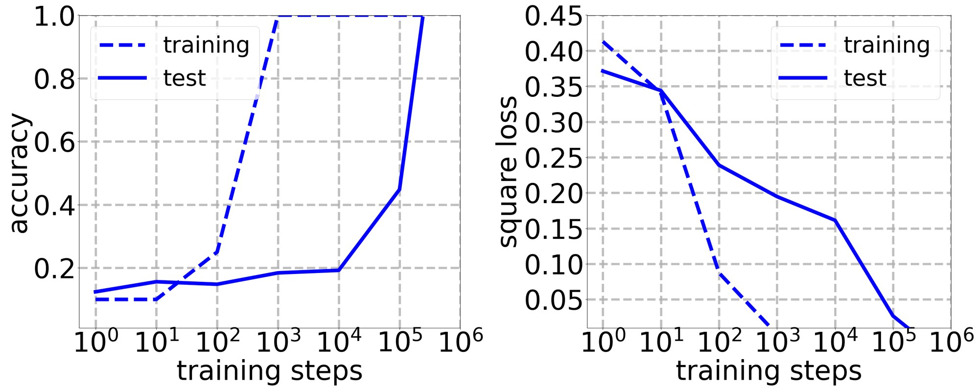
Figure 5: Plotting the grokking by evaluating the surrogate loss (an accuracy-type metric) compared to evaluating the actual loss. The data for the two plots are collected from a single simulation. We set , , , , and .
图 5:用替代损失(一种精度类指标)评估 grokking,并与用实际损失评估作比较。两幅图的数据来自同一次模拟。我们取 ,,,, 和 。
We also observe grokking in ridge regression with labels that are contaminated with mean-zero variance- Gaussian noise (Figure 6).
我们还在标签被均值为零、方差为 的高斯噪声污染的岭回归中观察到 grokking(图 6)。
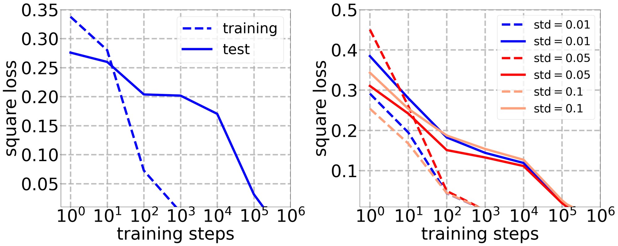
Figure 6: Ridge regression with label noise — Left: We set , , , , and ; Right: We notice that different noise levels do not affect the grokking time by much. We set , , , , and .
图 6:带标签噪声的岭回归——左:我们取 ,,,, 和 ;右:我们注意到,不同噪声水平对 grokking 时间影响不大。我们取 ,,,,以及 。
Finally, we observe grokking in the following setting. We study training a random Fourier feature network to learn a randomly-initialized realizable teacher. We implemented the random Fourier feature map where each row of is sampled from and each entry of is sampled from . Our randomly-initialized realizable teacher is a single such Fourier feature function generated from the same distribution. We note that this setting requires careful hyperparameter tuning to observe grokking (Figure 7).
最后,我们在如下设定中观察到 grokking。我们研究训练一个随机傅里叶特征网络,以学习一个随机初始化的可实现教师。我们实现随机傅里叶特征映射 ,其中 的每一行取自 , 的每个分量取自 。我们随机初始化的可实现教师,是从同一分布生成的单个这样的傅里叶特征函数。我们注意到,这一设定需要仔细调节超参数才能观察到 grokking(图 7)。
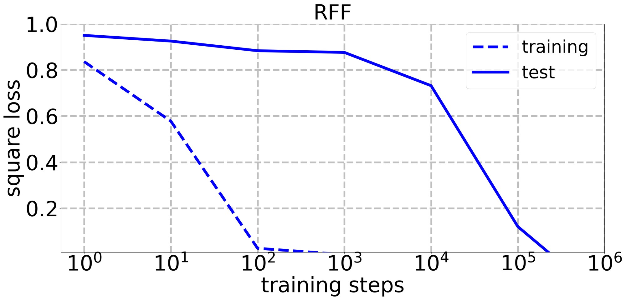
Figure 7: Random Fourier features — we set , , , , and .
图 7:随机傅里叶特征——我们取 ,,,, 和 。
Appendix C Technical Lemmas
附录 C 技术引理
Lemma C.1(Chi-squared Concentration).
引理 C.1(卡方集中)。
Let such that for some . For all ,
设 满足 ,其中 。对所有 ,