Inductive Representation Learning on Large Graphs
Inductive Representation Learning on Large Graphs
大规模图上的归纳式表示学习
William L. Hamilton † † thanks: The two first authors made equal contributions. Email: wleif@stanford.edu Rex Ying † † footnotemark: Email: rexying@stanford.edu Jure Leskovec Affiliation: jure@cs.stanford.edu Affiliation: Stanford University Affiliation: Stanford, CA, 94305
Abstract
摘要
Low-dimensional embeddings of nodes in large graphs have proved extremely useful in a variety of prediction tasks, from content recommendation to identifying protein functions. However, most existing approaches require that all nodes in the graph are present during training of the embeddings; these previous approaches are inherently transductive and do not naturally generalize to unseen nodes. Here we present GraphSAGE, a general inductive framework that leverages node feature information (e.g., text attributes) to efficiently generate node embeddings for previously unseen data. Instead of training individual embeddings for each node, we learn a function that generates embeddings by sampling and aggregating features from a node’s local neighborhood. Our algorithm outperforms strong baselines on three inductive node-classification benchmarks: we classify the category of unseen nodes in evolving information graphs based on citation and Reddit post data, and we show that our algorithm generalizes to completely unseen graphs using a multi-graph dataset of protein-protein interactions.
大规模图上节点的低维嵌入,在内容推荐到蛋白质功能识别等各类预测任务中已被证明极为有用。然而,现有方法大多要求训练嵌入时图中全部节点都已出现;这类做法本质上是直推式的,无法自然泛化到未见节点。本文提出 GraphSAGE:一种通用的归纳式框架,利用节点特征信息(例如文本属性),高效地为先前未见的数据生成节点嵌入。我们不为每个节点单独训练嵌入,而是学习一个函数:通过对节点局部邻域采样并聚合特征来生成嵌入。算法在三个归纳式节点分类基准上超过强基线:我们基于引文与 Reddit 帖子数据,对演化信息图中未见节点的类别做分类;并在蛋白质–蛋白质相互作用的多图数据集上表明,算法可泛化到完全未见的图。
1 Introduction
1 引言
Low-dimensional vector embeddings of nodes in large graphs have proved extremely useful as feature inputs for a wide variety of prediction and graph analysis tasks [5, 11, 28, 35, 36]. The basic idea behind node embedding approaches is to use dimensionality reduction techniques to distill the high-dimensional information about a node’s graph neighborhood into a dense vector embedding. These node embeddings can then be fed to downstream machine learning systems and aid in tasks such as node classification, clustering, and link prediction [11, 28, 35].
大规模图上节点的低维向量嵌入,作为特征输入,已被广泛用于各类预测与图分析任务 [5, 11, 28, 35, 36]。节点嵌入方法的基本思路是用降维技术,把节点图邻域的高维信息浓缩成稠密向量嵌入。这些嵌入可再交给下游机器学习系统,辅助节点分类、聚类与链路预测等任务 [11, 28, 35]。
However, previous works have focused on embedding nodes from a single fixed graph, and many real-world applications require embeddings to be quickly generated for unseen nodes, or entirely new (sub)graphs. This inductive capability is essential for high-throughput, production machine learning systems, which operate on evolving graphs and constantly encounter unseen nodes (e.g., posts on Reddit, users and videos on Youtube). An inductive approach to generating node embeddings also facilitates generalization across graphs with the same form of features: for example, one could train an embedding generator on protein-protein interaction graphs derived from a model organism, and then easily produce node embeddings for data collected on new organisms using the trained model.
然而,以往工作多聚焦于在单张固定图上嵌入节点,而许多现实应用需要为未见节点、乃至全新的(子)图快速生成嵌入。这种归纳能力对高吞吐的生产机器学习系统至关重要——它们运行在演化图上,不断遇到未见节点(例如 Reddit 上的帖子、YouTube 上的用户与视频)。归纳式生成节点嵌入,也便于在具有同种特征形式的图之间泛化:例如,可先在模式生物的蛋白质–蛋白质相互作用图上训练嵌入生成器,再用该模型为新生物上收集的数据直接产出节点嵌入。
The inductive node embedding problem is especially difficult, compared to the transductive setting, because generalizing to unseen nodes requires “aligning” newly observed subgraphs to the node embeddings that the algorithm has already optimized on. An inductive framework must learn to recognize structural properties of a node’s neighborhood that reveal both the node’s local role in the graph, as well as its global position.
与直推设定相比,归纳式节点嵌入尤其困难:泛化到未见节点,需要把新观测到的子图“对齐”到算法已在其上优化过的节点嵌入。归纳框架必须学会识别节点邻域的结构性质,这些性质既揭示节点在图中的局部角色,也反映其全局位置。
Most existing approaches to generating node embeddings are inherently transductive. The majority of these approaches directly optimize the embeddings for each node using matrix-factorization-based objectives, and do not naturally generalize to unseen data, since they make predictions on nodes in a single, fixed graph [5, 11, 23, 28, 35, 36, 37, 39]. These approaches can be modified to operate in an inductive setting (e.g., [28]), but these modifications tend to be computationally expensive, requiring additional rounds of gradient descent before new predictions can be made. There are also recent approaches to learning over graph structures using convolution operators that offer promise as an embedding methodology [17]. So far, graph convolutional networks (GCNs) have only been applied in the transductive setting with fixed graphs [17, 18]. In this work we both extend GCNs to the task of inductive unsupervised learning and propose a framework that generalizes the GCN approach to use trainable aggregation functions (beyond simple convolutions).
现有多数节点嵌入方法本质上是直推式的。它们大多用基于矩阵分解的目标直接优化每个节点的嵌入,由于预测仅针对单张固定图上的节点,无法自然泛化到未见数据 [5, 11, 23, 28, 35, 36, 37, 39]。这类方法可改造成归纳设定(例如 [28]),但改造往往计算昂贵,在做出新预测前还需要额外多轮梯度下降。也有近期工作用卷积算子在图结构上学习,有望成为嵌入方法 [17]。迄今为止,图卷积网络(GCN)只在固定图的直推设定中应用 [17, 18]。本文既把 GCN 扩展到归纳式无监督学习任务,也提出一个框架,把 GCN 思路推广到可训练的聚合函数(而不限于简单卷积)。
Present work. We propose a general framework, called GraphSAGE (sample and aggregate), for inductive node embedding. Unlike embedding approaches that are based on matrix factorization, we leverage node features (e.g., text attributes, node profile information, node degrees) in order to learn an embedding function that generalizes to unseen nodes. By incorporating node features in the learning algorithm, we simultaneously learn the topological structure of each node’s neighborhood as well as the distribution of node features in the neighborhood. While we focus on feature-rich graphs (e.g., citation data with text attributes, biological data with functional/molecular markers), our approach can also make use of structural features that are present in all graphs (e.g., node degrees). Thus, our algorithm can also be applied to graphs without node features.
本文工作。我们提出名为 GraphSAGE(采样与聚合,SAmple and aggreGatE)的通用归纳式节点嵌入框架。与基于矩阵分解的嵌入方法不同,我们利用节点特征(例如文本属性、节点画像信息、节点度数),学习一个可泛化到未见节点的嵌入函数。把节点特征纳入学习算法后,我们同时学到每个节点邻域的拓扑结构,以及邻域内节点特征的分布。我们聚焦特征丰富的图(例如带文本属性的引文数据、带功能/分子标记的生物数据),但方法也可利用所有图都具备的结构特征(例如节点度数)。因此,算法也能用于没有节点特征的图。
Instead of training a distinct embedding vector for each node, we train a set of aggregator functions that learn to aggregate feature information from a node’s local neighborhood (Figure ). Each aggregator function aggregates information from a different number of hops, or search depth, away from a given node. At test, or inference time, we use our trained system to generate embeddings for entirely unseen nodes by applying the learned aggregation functions. Following previous work on generating node embeddings, we design an unsupervised loss function that allows GraphSAGE to be trained without task-specific supervision. We also show that GraphSAGE can be trained in a fully supervised manner.
我们不为每个节点训练互异的嵌入向量,而是训练一组聚合函数,学会从节点局部邻域聚合特征信息(图)。每个聚合函数聚合距给定节点不同跳数(或搜索深度)的信息。在测试或推理时,用训练好的系统对完全未见的节点施加学到的聚合函数,即可生成嵌入。沿用此前节点嵌入工作,我们设计了无监督损失函数,使 GraphSAGE 可在没有任务特定监督时训练;同时也表明 GraphSAGE 可以完全监督的方式训练。
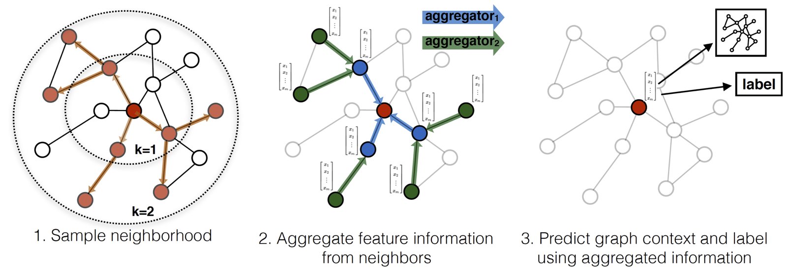
Figure 1: Visual illustration of the GraphSAGE sample and aggregate approach.
图 1:GraphSAGE 采样与聚合方法的示意。
We evaluate our algorithm on three node-classification benchmarks, which test GraphSAGE’s ability to generate useful embeddings on unseen data. We use two evolving document graphs based on citation data and Reddit post data (predicting paper and post categories, respectively), and a multi-graph generalization experiment based on a dataset of protein-protein interactions (predicting protein functions). Using these benchmarks, we show that our approach is able to effectively generate representations for unseen nodes and outperform relevant baselines by a significant margin: across domains, our supervised approach improves classification F1-scores by an average of 51% compared to using node features alone and GraphSAGE consistently outperforms a strong, transductive baseline [28], despite this baseline taking longer to run on unseen nodes. We also show that the new aggregator architectures we propose provide significant gains (7.4% on average) compared to an aggregator inspired by graph convolutional networks [17]. Lastly, we probe the expressive capability of our approach and show, through theoretical analysis, that GraphSAGE is capable of learning structural information about a node’s role in a graph, despite the fact that it is inherently based on features (Section ).
我们在三个节点分类基准上评估算法,检验 GraphSAGE 在未见数据上生成有用嵌入的能力。两个演化文档图分别基于引文数据与 Reddit 帖子数据(分别预测论文与帖子类别),另有一个基于蛋白质–蛋白质相互作用数据集的多图泛化实验(预测蛋白质功能)。在这些基准上,我们的方法能有效为未见节点生成表示,并以显著优势超过相关基线:跨领域平均来看,监督式方法相对仅用节点特征,分类 F1 提升约 51%;GraphSAGE 也持续超过一个强的直推基线 [28],尽管该基线在未见节点上运行约慢 。我们还表明,所提出的新聚合器结构相对受图卷积网络启发的聚合器平均再提升 7.4% [17]。最后,我们剖析方法的表达能力,并通过理论分析表明:尽管 GraphSAGE 本质上基于特征,仍能学到关于节点在图中角色的结构信息(第 节)。
2 Related work
2 相关工作
Our algorithm is conceptually related to previous node embedding approaches, general supervised approaches to learning over graphs, and recent advancements in applying convolutional neural networks to graph-structured data.
我们的算法在概念上与此前的节点嵌入方法、图上的一般监督学习方法,以及近期把卷积神经网络用于图结构数据的进展相关。
Factorization-based embedding approaches. There are a number of recent node embedding approaches that learn low-dimensional embeddings using random walk statistics and matrix factorization-based learning objectives [5, 11, 28, 35, 36]. These methods also bear close relationships to more classic approaches to spectral clustering [23], multi-dimensional scaling [19], as well as the PageRank algorithm [25]. Since these embedding algorithms directly train node embeddings for individual nodes, they are inherently transductive and, at the very least, require expensive additional training (e.g., via stochastic gradient descent) to make predictions on new nodes. In addition, for many of these approaches (e.g., [11, 28, 35, 36]) the objective function is invariant to orthogonal transformations of the embeddings, which means that the embedding space does not naturally generalize between graphs and can drift during re-training. One notable exception to this trend is the Planetoid-I algorithm introduced by Yang et al. [40], which is an inductive, embedding-based approach to semi-supervised learning. However, Planetoid-I does not use any graph structural information during inference; instead, it uses the graph structure as a form of regularization during training. Unlike these previous approaches, we leverage feature information in order to train a model to produce embeddings for unseen nodes.
基于分解的嵌入方法。近期有一批节点嵌入方法,用随机游走统计量与基于矩阵分解的学习目标来学习低维嵌入 [5, 11, 28, 35, 36]。它们也与更经典的谱聚类 [23]、多维尺度变换 [19] 以及 PageRank 算法 [25] 关系密切。由于这些算法直接为每个节点训练嵌入,本质上是直推式的;至少也需要昂贵的额外训练(例如通过随机梯度下降)才能对新节点做预测。此外,对其中许多方法(例如 [11, 28, 35, 36]),目标函数对嵌入的正交变换不变,这意味着嵌入空间不会在图之间自然泛化,并可能在重训时漂移。一个值得注意的例外是 Yang 等人提出的 Planetoid-I [40]:它是一种归纳式、基于嵌入的半监督学习方法。但 Planetoid-I 在推理时不使用任何图结构信息;图结构只在训练时作为正则。与这些先前方法不同,我们利用特征信息,训练一个能为未见节点产出嵌入的模型。
Supervised learning over graphs. Beyond node embedding approaches, there is a rich literature on supervised learning over graph-structured data. This includes a wide variety of kernel-based approaches, where feature vectors for graphs are derived from various graph kernels (see [32] and references therein). There are also a number of recent neural network approaches to supervised learning over graph structures [7, 10, 21, 31]. Our approach is conceptually inspired by a number of these algorithms. However, whereas these previous approaches attempt to classify entire graphs (or subgraphs), the focus of this work is generating useful representations for individual nodes.
图上的监督学习。在节点嵌入之外,图结构数据上的监督学习文献也很丰富。其中包括大量基于核的方法:图的特征向量由各类图核导出(见 [32] 及其引用)。也有一批近期用神经网络在图结构上做监督学习的工作 [7, 10, 21, 31]。我们的方法在概念上受其中若干算法启发。不过,这些先前工作试图分类整张图(或子图),而本文的重点是为单个节点生成有用表示。
Graph convolutional networks. In recent years, several convolutional neural network architectures for learning over graphs have been proposed (e.g., [4, 9, 8, 17, 24]). The majority of these methods do not scale to large graphs or are designed for whole-graph classification (or both) [4, 9, 8, 24]. However, our approach is closely related to the graph convolutional network (GCN), introduced by Kipf et al. [17, 18]. The original GCN algorithm [17] is designed for semi-supervised learning in a transductive setting, and the exact algorithm requires that the full graph Laplacian is known during training. A simple variant of our algorithm can be viewed as an extension of the GCN framework to the inductive setting, a point which we revisit in Section .
图卷积网络。近年来,已有若干面向图学习的卷积神经网络结构被提出(例如 [4, 9, 8, 17, 24])。其中多数无法扩展到大图,或面向整图分类(或两者皆是)[4, 9, 8, 24]。不过,我们的方法与 Kipf 等人提出的图卷积网络(GCN)密切相关 [17, 18]。原始 GCN 算法 [17] 面向直推设定下的半监督学习,精确算法要求训练时已知完整图拉普拉斯。我们算法的一个简单变体,可视为把 GCN 框架扩展到归纳设定;这一点我们在第 节还会回到。
3 Proposed method: GraphSAGE
3 方法:GraphSAGE
The key idea behind our approach is that we learn how to aggregate feature information from a node’s local neighborhood (e.g., the degrees or text attributes of nearby nodes). We first describe the GraphSAGE embedding generation (i.e., forward propagation) algorithm, which generates embeddings for nodes assuming that the GraphSAGE model parameters are already learned (Section ). We then describe how the GraphSAGE model parameters can be learned using standard stochastic gradient descent and backpropagation techniques (Section ).
方法的核心思想是:学习如何从节点局部邻域聚合特征信息(例如邻近节点的度数或文本属性)。我们先描述 GraphSAGE 的嵌入生成(即前向传播)算法——假定 GraphSAGE 模型参数已学好,如何为节点生成嵌入(第 节);再说明如何用标准随机梯度下降与反向传播学习这些参数(第 节)。
3.1 Embedding generation (i.e., forward propagation) algorithm
3.1 嵌入生成(即前向传播)算法
Input : Graph ; input features ; depth ; weight matrices ; non-linearity ; differentiable aggregator functions ; neighborhood function
Output : Vector representations for all
1 ;
2 for do
3 for do
4 ;
5
6 end for
7
8 end for
9
Algorithm 1 GraphSAGE embedding generation (i.e., forward propagation) algorithm
输入: 图 ;输入特征 ;深度 ;权重矩阵 ;非线性 ;可微聚合函数 ;邻域函数
输出: 所有 的向量表示
1 ;
2 for do
3 for do
4 ;
5
6 end for
7
8 end for
9
算法 1 GraphSAGE 嵌入生成(即前向传播)算法
In this section, we describe the embedding generation, or forward propagation algorithm (Algorithm ), which assumes that the model has already been trained and that the parameters are fixed. In particular, we assume that we have learned the parameters of aggregator functions (denoted ), which aggregate information from node neighbors, as well as a set of weight matrices , which are used to propagate information between different layers of the model or “search depths”. Section describes how we train these parameters.
本节描述嵌入生成(即前向传播)算法(算法),假定模型已训练完毕、参数固定。具体而言,假定我们已学到 个聚合函数的参数(记为 ),它们聚合来自节点邻居的信息;以及一组权重矩阵 ,用于在模型不同层或“搜索深度”之间传播信息。第 节说明如何训练这些参数。
The intuition behind Algorithm is that at each iteration, or search depth, nodes aggregate information from their local neighbors, and as this process iterates, nodes incrementally gain more and more information from further reaches of the graph.
算法 背后的直觉是:在每次迭代(或搜索深度),节点从其局部邻居聚合信息;随着过程迭代,节点逐步获得来自图更远处的信息。
Algorithm describes the embedding generation process in the case where the entire graph, , and features for all nodes , are provided as input. We describe how to generalize this to the minibatch setting below. Each step in the outer loop of Algorithm proceeds as follows, where denotes the current step in the outer loop (or the depth of the search) and denotes a node’s representation at this step: First, each node aggregates the representations of the nodes in its immediate neighborhood, , into a single vector . Note that this aggregation step depends on the representations generated at the previous iteration of the outer loop (i.e., ), and the (“base case”) representations are defined as the input node features. After aggregating the neighboring feature vectors, GraphSAGE then concatenates the node’s current representation, , with the aggregated neighborhood vector, , and this concatenated vector is fed through a fully connected layer with nonlinear activation function , which transforms the representations to be used at the next step of the algorithm (i.e., ). For notational convenience, we denote the final representations output at depth as . The aggregation of the neighbor representations can be done by a variety of aggregator architectures (denoted by the aggregate placeholder in Algorithm 1), and we discuss different architecture choices in Section below.
算法 描述的是整张图 以及所有节点特征 都作为输入给出时的嵌入生成过程。下文再说明如何推广到小批量设定。算法外层循环的每一步如下,其中 表示外层循环当前步(或搜索深度), 表示该步的节点表示:首先,每个节点 把其直接邻域中节点的表示 聚合成单个向量 。注意该聚合步依赖于外层循环上一轮(即 )生成的表示,(“基准情形”)的表示定义为输入节点特征。聚合邻域特征向量后,GraphSAGE 再把节点当前表示 与聚合后的邻域向量 拼接,并将拼接向量送入带非线性激活 的全连接层,变换得到算法下一步要用的表示(即 )。为记法方便,把深度 输出的最终表示记为 。邻居表示的聚合可由多种聚合器结构完成(算法 1 中用 aggregate 占位符表示),不同结构选择见下文第 节。
To extend Algorithm to the minibatch setting, given a set of input nodes, we first forward sample the required neighborhood sets (up to depth ) and then we run the inner loop (line 3 in Algorithm ), but instead of iterating over all nodes, we compute only the representations that are necessary to satisfy the recursion at each depth (Appendix contains complete minibatch pseudocode).
要把算法 扩展到小批量设定:给定一组输入节点,先前向采样所需的邻域集合(直到深度 ),再运行内层循环(算法 第 3 行);但不是遍历所有节点,而只计算满足每层递归所需的那些表示(附录给出完整小批量伪代码)。
Relation to the Weisfeiler-Lehman Isomorphism Test. The GraphSAGE algorithm is conceptually inspired by a classic algorithm for testing graph isomorphism. If, in Algorithm , we (i) set , (ii) set the weight matrices as the identity, and (iii) use an appropriate hash function as an aggregator (with no non-linearity), then Algorithm is an instance of the Weisfeiler-Lehman (WL) isomorphism test, also known as “naive vertex refinement” [32]. If the set of representations output by Algorithm for two subgraphs are identical then the WL test declares the two subgraphs to be isomorphic. This test is known to fail in some cases, but is valid for a broad class of graphs [32]. GraphSAGE is a continuous approximation to the WL test, where we replace the hash function with trainable neural network aggregators. Of course, we use GraphSAGE to generate useful node representations–not to test graph isomorphism. Nevertheless, the connection between GraphSAGE and the classic WL test provides theoretical context for our algorithm design to learn the topological structure of node neighborhoods.
与 Weisfeiler-Lehman 同构检验的关系。GraphSAGE 算法在概念上受经典图同构检验算法启发。若在算法 中我们 (i) 取 ,(ii) 把权重矩阵设为单位阵,(iii) 用合适的哈希函数作聚合器(且无非线性),则算法 就是 Weisfeiler-Lehman(WL)同构检验的一个实例,也称为“朴素顶点细化”[32]。若算法 对两个子图输出的表示集合 相同,则 WL 检验宣告这两个子图同构。该检验在某些情形会失败,但对广泛一类图是有效的 [32]。GraphSAGE 是 WL 检验的连续近似:我们用可训练的神经网络聚合器替换哈希函数。当然,我们用 GraphSAGE 是为生成有用的节点表示,而非检验图同构。尽管如此,GraphSAGE 与经典 WL 检验的联系,为我们设计算法以学习节点邻域拓扑结构提供了理论语境。
Neighborhood definition. In this work, we uniformly sample a fixed-size set of neighbors, instead of using full neighborhood sets in Algorithm , in order to keep the computational footprint of each batch fixed. That is, using overloaded notation, we define as a fixed-size, uniform draw from the set , and we draw different uniform samples at each iteration, , in Algorithm . Without this sampling the memory and expected runtime of a single batch is unpredictable and in the worst case . In contrast, the per-batch space and time complexity for GraphSAGE is fixed at , where and are user-specified constants. Practically speaking we found that our approach could achieve high performance with and (see Section for details).
邻域定义。本文不在算法 中使用完整邻域集合,而是均匀采样固定大小的邻居集合,以使每批的计算足迹固定。也就是说,我们重载记号,把 定义为从集合 中均匀抽取的固定大小样本,并在算法 的每次迭代 重新独立均匀抽样。若不做采样,单批的内存与期望运行时间不可预测,最坏情形为 。相比之下,GraphSAGE 每批的空间与时间复杂度固定为 ,其中 与 均为用户指定常数。实践中我们发现, 且 即可达到高性能(细节见第 节)。
3.2 Learning the parameters of GraphSAGE
3.2 学习 GraphSAGE 的参数
In order to learn useful, predictive representations in a fully unsupervised setting, we apply a graph-based loss function to the output representations, , and tune the weight matrices, , and parameters of the aggregator functions via stochastic gradient descent. The graph-based loss function encourages nearby nodes to have similar representations, while enforcing that the representations of disparate nodes are highly distinct:
为了在完全无监督设定下学到有用、可预测的表示,我们对输出表示 施加基于图的损失函数,并通过随机梯度下降调节权重矩阵 以及聚合函数的参数。该基于图的损失鼓励邻近节点具有相似表示,同时迫使相距较远节点的表示高度可分:
where is a node that co-occurs near on fixed-length random walk, is the sigmoid function, is a negative sampling distribution, and defines the number of negative samples. Importantly, unlike previous embedding approaches, the representations that we feed into this loss function are generated from the features contained within a node’s local neighborhood, rather than training a unique embedding for each node (via an embedding look-up).
其中 是固定长度随机游走中与 共同出现在附近的节点, 为 sigmoid 函数, 为负采样分布, 为负样本数。重要的是,与以往嵌入方法不同,我们送入该损失的表示 由节点局部邻域内所含特征生成,而不是(通过嵌入查找表)为每个节点训练唯一嵌入。
This unsupervised setting emulates situations where node features are provided to downstream machine learning applications, as a service or in a static repository. In cases where representations are to be used only on a specific downstream task, the unsupervised loss (Equation ) can simply be replaced, or augmented, by a task-specific objective (e.g., cross-entropy loss).
这一无监督设定模拟了把节点特征作为服务或静态仓库提供给下游机器学习应用的情形。若表示只用于特定下游任务,则可用任务特定目标(例如交叉熵损失)简单替换或增强无监督损失(方程)。
3.3 Aggregator Architectures
3.3 聚合器结构
Unlike machine learning over N-D lattices (e.g., sentences, images, or 3-D volumes), a node’s neighbors have no natural ordering; thus, the aggregator functions in Algorithm must operate over an unordered set of vectors. Ideally, an aggregator function would be symmetric (i.e., invariant to permutations of its inputs) while still being trainable and maintaining high representational capacity. The symmetry property of the aggregation function ensures that our neural network model can be trained and applied to arbitrarily ordered node neighborhood feature sets. We examined three candidate aggregator functions:
与在 N 维格点(例如句子、图像或三维体)上的机器学习不同,节点的邻居没有天然顺序;因此算法 中的聚合函数必须作用于无序向量集合。理想情况下,聚合函数应是对称的(即对输入置换不变),同时仍可训练并保持高表示能力。聚合函数的对称性保证神经网络模型能在任意排序的节点邻域特征集合上训练与应用。我们考察了三种候选聚合函数:
Mean aggregator. Our first candidate aggregator function is the mean operator, where we simply take the elementwise mean of the vectors in . The mean aggregator is nearly equivalent to the convolutional propagation rule used in the transductive GCN framework [17]. In particular, we can derive an inductive variant of the GCN approach by replacing lines 4 and 5 in Algorithm with the following:
均值聚合器。第一种候选是均值算子:对集合 中的向量取逐元素均值。均值聚合器与直推式 GCN 框架中使用的卷积传播规则几乎等价 [17]。具体地,若把算法 第 4、5 行替换为下式,即可导出 GCN 方法的归纳变体:
We call this modified mean-based aggregator convolutional since it is a rough, linear approximation of a localized spectral convolution [17]. An important distinction between this convolutional aggregator and our other proposed aggregators is that it does not perform the concatenation operation in line 5 of Algorithm —i.e., the convolutional aggregator does concatenate the node’s previous layer representation with the aggregated neighborhood vector . This concatenation can be viewed as a simple form of a “skip connection” [13] between the different “search depths”, or “layers” of the GraphSAGE algorithm, and it leads to significant gains in performance (Section ).
我们称这一改写后的基于均值的聚合器为卷积式聚合器,因为它是局部谱卷积的一种粗糙线性近似 [17]。该卷积聚合器与我们提出的其他聚合器的一个重要区别是:它不执行算法 第 5 行的拼接操作——即卷积聚合器并不把节点上一层表示 与聚合邻域向量 拼接。该拼接可视为 GraphSAGE 算法不同“搜索深度”或“层”之间一种简单的“跳跃连接”[13],并能带来显著性能提升(第 节)。
LSTM aggregator. We also examined a more complex aggregator based on an LSTM architecture [14]. Compared to the mean aggregator, LSTMs have the advantage of larger expressive capability. However, it is important to note that LSTMs are not inherently symmetric (i.e., they are not permutation invariant), since they process their inputs in a sequential manner. We adapt LSTMs to operate on an unordered set by simply applying the LSTMs to a random permutation of the node’s neighbors.
LSTM 聚合器。我们也考察了基于 LSTM 结构的更复杂聚合器 [14]。相对均值聚合器,LSTM 的优势是表达能力更大。但需注意 LSTM 本身并不对称(即不具置换不变性),因为它们按序列方式处理输入。我们通过对节点邻居的随机置换应用 LSTM,使其能作用于无序集合。
Pooling aggregator. The final aggregator we examine is both symmetric and trainable. In this pooling approach, each neighbor’s vector is independently fed through a fully-connected neural network; following this transformation, an elementwise max-pooling operation is applied to aggregate information across the neighbor set:
池化聚合器。我们考察的最后一种聚合器既对称又可训练。在这一池化方法中,每个邻居的向量先独立通过全连接神经网络;变换后再用逐元素最大池化跨邻居集合聚合信息:
where denotes the element-wise max operator and is a nonlinear activation function. In principle, the function applied before the max pooling can be an arbitrarily deep multi-layer perceptron, but we focus on simple single-layer architectures in this work. This approach is inspired by recent advancements in applying neural network architectures to learn over general point sets [29]. Intuitively, the multi-layer perceptron can be thought of as a set of functions that compute features for each of the node representations in the neighbor set. By applying the max-pooling operator to each of the computed features, the model effectively captures different aspects of the neighborhood set. Note also that, in principle, any symmetric vector function could be used in place of the operator (e.g., an element-wise mean). We found no significant difference between max- and mean-pooling in developments test and thus focused on max-pooling for the rest of our experiments.
其中 表示逐元素最大算子, 为非线性激活。原则上,最大池化前的函数可以是任意深的多层感知机,但本文聚焦简单的单层结构。该方法受近期把神经网络用于一般点集学习的进展启发 [29]。直观上,多层感知机可视为一组为邻域集合中每个节点表示计算特征的函数。对每个计算得到的特征施加最大池化,模型就能有效捕捉邻域集合的不同侧面。原则上,也可用任何对称的向量函数替换 算子(例如逐元素均值)。在开发测试中,我们发现最大池化与均值池化无显著差异,因此后续实验聚焦最大池化。
4 Experiments
4 实验
We test the performance of GraphSAGE on three benchmark tasks: (i) classifying academic papers into different subjects using the Web of Science citation dataset, (ii) classifying Reddit posts as belonging to different communities, and (iii) classifying protein functions across various biological protein-protein interaction (PPI) graphs. Sections and summarize the datasets, and the supplementary material contains additional information. In all these experiments, we perform predictions on nodes that are not seen during training, and, in the case of the PPI dataset, we test on entirely unseen graphs.
我们在三项基准任务上测试 GraphSAGE:(i) 用 Web of Science 引文数据集把学术论文分到不同学科;(ii) 把 Reddit 帖子分到不同社区;(iii) 在多张生物蛋白质–蛋白质相互作用(PPI)图上分类蛋白质功能。第 节与第 节概述数据集,补充材料含更多信息。所有这些实验中,我们都对训练时未见的节点做预测;在 PPI 数据集上,还在完全未见的图上测试。
Experimental set-up. To contextualize the empirical results on our inductive benchmarks, we compare against four baselines: a random classifer, a logistic regression feature-based classifier (that ignores graph structure), the DeepWalk algorithm [28] as a representative factorization-based approach, and a concatenation of the raw features and DeepWalk embeddings. We also compare four variants of GraphSAGE that use the different aggregator functions (Section ). Since, the “convolutional” variant of GraphSAGE is an extended, inductive version of Kipf et al’s semi-supervised GCN [17], we term this variant GraphSAGE-GCN. We test unsupervised variants of GraphSAGE trained according to the loss in Equation (), as well as supervised variants that are trained directly on classification cross-entropy loss. For all the GraphSAGE variants we used rectified linear units as the non-linearity and set with neighborhood sample sizes and (see Section for sensitivity analyses).
实验设置。为给归纳基准上的实证结果提供语境,我们对比四个基线:随机分类器、忽略图结构的逻辑回归特征分类器、作为基于分解方法代表的 DeepWalk 算法 [28],以及原始特征与 DeepWalk 嵌入的拼接。我们也对比使用不同聚合函数的四种 GraphSAGE 变体(第 节)。由于 GraphSAGE 的“卷积”变体是 Kipf 等人半监督 GCN [17] 的扩展归纳版本,我们称之为 GraphSAGE-GCN。我们测试按方程 () 损失训练的无监督 GraphSAGE 变体,以及直接在分类交叉熵损失上训练的监督变体。对所有 GraphSAGE 变体,非线性用修正线性单元,取 ,邻域采样大小 、(敏感性分析见第 节)。
For the Reddit and citation datasets, we use “online” training for DeepWalk as described in Perozzi et al. [28], where we run a new round of SGD optimization to embed the new test nodes before making predictions (see the Appendix for details). In the multi-graph setting, we cannot apply DeepWalk, since the embedding spaces generated by running the DeepWalk algorithm on different disjoint graphs can be arbitrarily rotated with respect to each other (Appendix ).
对 Reddit 与引文数据集,我们按 Perozzi 等人 [28] 所述对 DeepWalk 做“在线”训练:在做预测前,对新测试节点再跑一轮 SGD 优化以嵌入它们(细节见附录)。在多图设定下无法应用 DeepWalk,因为在不同不交图上运行 DeepWalk 得到的嵌入空间可彼此任意旋转(附录)。
All models were implemented in TensorFlow [1] with the Adam optimizer [16] (except DeepWalk, which performed better with the vanilla gradient descent optimizer). We designed our experiments with the goals of (i) verifying the improvement of GraphSAGE over the baseline approaches (i.e., raw features and DeepWalk) and (ii) providing a rigorous comparison of the different GraphSAGE aggregator architectures. In order to provide a fair comparison, all models share an identical implementation of their minibatch iterators, loss function and neighborhood sampler (when applicable). Moreover, in order to guard against unintentional “hyperparameter hacking” in the comparisons between GraphSAGE aggregators, we sweep over the same set of hyperparameters for all GraphSAGE variants (choosing the best setting for each variant according to performance on a validation set). The set of possible hyperparameter values was determined on early validation tests using subsets of the citation and Reddit data that we then discarded from our analyses. The appendix contains further implementation details.
除 DeepWalk(用普通梯度下降效果更好)外,所有模型均在 TensorFlow [1] 中实现,并用 Adam 优化器 [16]。实验设计目标是:(i) 验证 GraphSAGE 相对基线方法(即原始特征与 DeepWalk)的提升;(ii) 对不同 GraphSAGE 聚合器结构做严格比较。为公平比较,所有模型共享相同的小批量迭代器、损失函数与邻域采样器实现(适用时)。此外,为防止 GraphSAGE 聚合器比较中无意的“超参作弊”,我们对所有 GraphSAGE 变体扫描同一组超参(按验证集表现为每个变体选最佳设置)。可能的超参取值集合在早期验证测试中、用随后从分析中剔除的引文与 Reddit 数据子集上确定。附录含更多实现细节。
4.1 Inductive learning on evolving graphs: Citation and Reddit data
4.1 演化图上的归纳学习:引文与 Reddit 数据
| Citation | PPI | |||||
|---|---|---|---|---|---|---|
| Name | Unsup. F1 | Sup. F1 | Unsup. F1 | Sup. F1 | Unsup. F1 | Sup. F1 |
| Random | 0.206 | 0.206 | 0.043 | 0.042 | 0.396 | 0.396 |
| Raw features | 0.575 | 0.575 | 0.585 | 0.585 | 0.422 | 0.422 |
| DeepWalk | 0.565 | 0.565 | 0.324 | 0.324 | — | — |
| DeepWalk + features | 0.701 | 0.701 | 0.691 | 0.691 | — | — |
| GraphSAGE-GCN | 0.742 | 0.772 | 0.908 | 0.930 | 0.465 | 0.500 |
| GraphSAGE-mean | 0.778 | 0.820 | 0.897 | 0.950 | 0.486 | 0.598 |
| GraphSAGE-LSTM | 0.788 | 0.832 | 0.907 | 0.954 | 0.482 | 0.612 |
| GraphSAGE-pool | 0.798 | 0.839 | 0.892 | 0.948 | 0.502 | 0.600 |
| % gain over feat. | 39% | 46% | 55% | 63% | 19% | 45% |
Table 1: Prediction results for the three datasets (micro-averaged F1 scores). Results for unsupervised and fully supervised GraphSAGE are shown. Analogous trends hold for macro-averaged scores.
| 引文 | PPI | |||||
|---|---|---|---|---|---|---|
| 名称 | 无监督 F1 | 监督 F1 | 无监督 F1 | 监督 F1 | 无监督 F1 | 监督 F1 |
| Random | 0.206 | 0.206 | 0.043 | 0.042 | 0.396 | 0.396 |
| Raw features | 0.575 | 0.575 | 0.585 | 0.585 | 0.422 | 0.422 |
| DeepWalk | 0.565 | 0.565 | 0.324 | 0.324 | — | — |
| DeepWalk + features | 0.701 | 0.701 | 0.691 | 0.691 | — | — |
| GraphSAGE-GCN | 0.742 | 0.772 | 0.908 | 0.930 | 0.465 | 0.500 |
| GraphSAGE-mean | 0.778 | 0.820 | 0.897 | 0.950 | 0.486 | 0.598 |
| GraphSAGE-LSTM | 0.788 | 0.832 | 0.907 | 0.954 | 0.482 | 0.612 |
| GraphSAGE-pool | 0.798 | 0.839 | 0.892 | 0.948 | 0.502 | 0.600 |
| 相对特征的增益 % | 39% | 46% | 55% | 63% | 19% | 45% |
表 1:三个数据集上的预测结果(微平均 F1)。给出无监督与完全监督 GraphSAGE 的结果。宏平均分数呈现类似趋势。
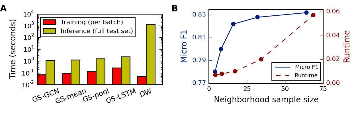
Figure 2: A: Timing experiments on Reddit data, with training batches of size 512 and inference on the full test set (79,534 nodes). B: Model performance with respect to the size of the sampled neighborhood, where the “neighborhood sample size” refers to the number of neighbors sampled at each depth for with (on the citation data using GraphSAGE-mean).
图 2:A:Reddit 数据上的计时实验,训练批大小 512,在完整测试集(79,534 个节点)上推理。B:模型表现相对采样邻域大小的变化;“邻域采样大小”指 且 时每层采样的邻居数(引文数据,GraphSAGE-mean)。
Our first two experiments are on classifying nodes in evolving information graphs, a task that is especially relevant to high-throughput production systems, which constantly encounter unseen data.
前两个实验是在演化信息图上对节点分类,这一任务对不断遇到未见数据的高吞吐生产系统尤其相关。
Citation data. Our first task is predicting paper subject categories on a large citation dataset. We use an undirected citation graph dataset derived from the Thomson Reuters Web of Science Core Collection, corresponding to all papers in six biology-related fields for the years 2000-2005. The node labels for this dataset correspond to the six different field labels. In total, this is dataset contains 302,424 nodes with an average degree of 9.15. We train all the algorithms on the 2000-2004 data and use the 2005 data for testing (with 30% used for validation). For features, we used node degrees and processed the paper abstracts according Arora et al.’s [2] sentence embedding approach, with 300-dimensional word vectors trained using the GenSim word2vec implementation [30].
引文数据。第一项任务是在大型引文数据集上预测论文学科类别。我们使用源自 Thomson Reuters Web of Science Core Collection 的无向引文图,对应 2000–2005 年六个生物学相关领域的全部论文。节点标签即这六个领域标签。该数据集共 302,424 个节点,平均度数 9.15。所有算法在 2000–2004 年数据上训练,用 2005 年数据测试(其中 30% 作验证)。特征方面,我们使用节点度数,并按 Arora 等人 [2] 的句子嵌入方法处理论文摘要,词向量为用 GenSim word2vec 实现 [30] 训练的 300 维。
Reddit data. In our second task, we predict which community different Reddit posts belong to. Reddit is a large online discussion forum where users post and comment on content in different topical communities. We constructed a graph dataset from Reddit posts made in the month of September, 2014. The node label in this case is the community, or “subreddit”, that a post belongs to. We sampled 50 large communities and built a post-to-post graph, connecting posts if the same user comments on both. In total this dataset contains 232,965 posts with an average degree of 492. We use the first 20 days for training and the remaining days for testing (with 30% used for validation). For features, we use off-the-shelf 300-dimensional GloVe CommonCrawl word vectors [27]; for each post, we concatenated (i) the average embedding of the post title, (ii) the average embedding of all the post’s comments (iii) the post’s score, and (iv) the number of comments made on the post.
Reddit 数据。第二项任务预测不同 Reddit 帖子属于哪个社区。Reddit 是大型在线讨论论坛,用户在不同主题社区发帖与评论。我们从 2014 年 9 月的 Reddit 帖子构建图数据集。节点标签为帖子所属社区(即 “subreddit”)。我们采样 50 个大型社区,构建帖子–帖子图:若同一用户对两篇帖子都发表评论,则连接这两篇帖子。该数据集共 232,965 篇帖子,平均度数 492。前 20 天用于训练,其余天用于测试(其中 30% 作验证)。特征使用现成的 300 维 GloVe CommonCrawl 词向量 [27];对每篇帖子,我们拼接 (i) 标题的平均嵌入,(ii) 该帖全部评论的平均嵌入,(iii) 帖子得分,以及 (iv) 帖子评论数。
The first four columns of Table summarize the performance of GraphSAGE as well as the baseline approaches on these two datasets. We find that GraphSAGE outperforms all the baselines by a significant margin, and the trainable, neural network aggregators provide significant gains compared to the GCN approach. For example, the unsupervised variant GraphSAGE-pool outperforms the concatenation of the DeepWalk embeddings and the raw features by 13.8% on the citation data and 29.1% on the Reddit data, while the supervised version provides a gain of 19.7% and 37.2%, respectively. Interestingly, the LSTM based aggregator shows strong performance, despite the fact that it is designed for sequential data and not unordered sets. Lastly, we see that the performance of unsupervised GraphSAGE is reasonably competitive with the fully supervised version, indicating that our framework can achieve strong performance without task-specific fine-tuning.
表 前四列总结了 GraphSAGE 与基线方法在这两个数据集上的表现。我们发现 GraphSAGE 以显著优势超过所有基线,且可训练的神经网络聚合器相对 GCN 方法带来显著增益。例如,无监督变体 GraphSAGE-pool 相对 DeepWalk 嵌入与原始特征的拼接,在引文数据上高 13.8%,在 Reddit 数据上高 29.1%;监督版本的增益分别为 19.7% 与 37.2%。有趣的是,基于 LSTM 的聚合器表现也很强,尽管它面向序列数据而非无序集合。最后,无监督 GraphSAGE 的表现与完全监督版本具有合理竞争力,表明我们的框架无需任务特定微调也能取得强表现。
4.2 Generalizing across graphs: Protein-protein interactions
4.2 跨图泛化:蛋白质–蛋白质相互作用
We now consider the task of generalizing across graphs, which requires learning about node roles rather than community structure. We classify protein roles—in terms of their cellular functions from gene ontology—in various protein-protein interaction (PPI) graphs, with each graph corresponding to a different human tissue [41]. We use positional gene sets, motif gene sets and immunological signatures as features and gene ontology sets as labels (121 in total), collected from the Molecular Signatures Database [34]. The average graph contains 2373 nodes, with an average degree of 28.8. We train all algorithms on 20 graphs and then average prediction F1 scores on two test graphs (with two other graphs used for validation).
我们现在考虑跨图泛化任务,这要求学习节点角色而非社区结构。我们按基因本体中的细胞功能,在多张蛋白质–蛋白质相互作用(PPI)图上分类蛋白质角色,每张图对应不同人体组织 [41]。特征使用位置基因集、基序基因集与免疫签名,标签为基因本体集合(共 121 个),均来自 Molecular Signatures Database [34]。平均每张图有 2373 个节点,平均度数 28.8。所有算法在 20 张图上训练,再在两张测试图上平均预测 F1(另两张图作验证)。
The final two columns of Table summarize the accuracies of the various approaches on this data. Again we see that GraphSAGE significantly outperforms the baseline approaches, with the LSTM- and pooling-based aggregators providing substantial gains over the mean- and GCN-based aggregators.
表 最后两列总结了各方法在该数据上的准确率。我们再次看到 GraphSAGE 显著超过基线;基于 LSTM 与池化的聚合器相对基于均值与 GCN 的聚合器带来可观增益。
4.3 Runtime and parameter sensitivity
4.3 运行时间与参数敏感性
Figure .A summarizes the training and test runtimes for the different approaches. The training time for the methods are comparable (with GraphSAGE-LSTM being the slowest). However, the need to sample new random walks and run new rounds of SGD to embed unseen nodes makes DeepWalk slower at test time.
图 .A 总结了不同方法的训练与测试运行时间。各方法训练时间相当(GraphSAGE-LSTM 最慢)。但为嵌入未见节点需采样新的随机游走并再跑多轮 SGD,使 DeepWalk 在测试时慢 。
For the GraphSAGE variants, we found that setting provided a consistent boost in accuracy of around , on average, compared to ; however, increasing beyond 2 gave marginal returns in performance () while increasing the runtime by a prohibitively large factor of , depending on the neighborhood sample size. We also found diminishing returns for sampling large neighborhoods (Figure .B). Thus, despite the higher variance induced by sub-sampling neighborhoods, GraphSAGE is still able to maintain strong predictive accuracy, while significantly improving the runtime.
对 GraphSAGE 变体,我们发现相对 ,设 平均可稳定提升准确率约 ;但把 增到超过 2 收益有限(),运行时间却会按邻域采样大小放大到令人望而却步的 。采样大邻域也呈现收益递减(图 .B)。因此,尽管子采样邻域会带来更高方差,GraphSAGE 仍能保持强预测准确率,同时显著改善运行时间。
4.4 Summary comparison between the different aggregator architectures
4.4 不同聚合器结构的总结比较
Overall, we found that the LSTM- and pool-based aggregators performed the best, in terms of both average performance and number of experimental settings where they were the top-performing method (Table ). To give more quantitative insight into these trends, we consider each of the six different experimental settings (i.e., ) as trials and consider what performance trends are likely to generalize. In particular, we use the non-parametric Wilcoxon Signed-Rank Test [33] to quantify the differences between the different aggregators across trials, reporting the -statistic and -value where applicable. Note that this method is rank-based and essentially tests whether we would expect one particular approach to outperform another in a new experimental setting. Given our small sample size of only 6 different settings, this significance test is somewhat underpowered; nonetheless, the -statistic and associated -values are useful quantitative measures to assess the aggregators’ relative performances.
总体而言,我们发现基于 LSTM 与池化的聚合器表现最好,无论是平均表现,还是成为最佳方法的实验设置数量(表)。为更定量地洞察这些趋势,我们把六种不同实验设置(即 )各视为一次试验,考察何种表现趋势可能泛化。具体地,我们用非参数 Wilcoxon 符号秩检验 [33] 量化不同聚合器跨试验的差异,并在适用时报告 统计量与 值。该方法基于秩,本质上检验:在新的实验设置中,我们是否会期望某一方法超过另一方法。鉴于只有 6 种设置的小样本量,这一显著性检验功效偏弱;尽管如此, 统计量与相应 值仍是评估聚合器相对表现的有用定量指标。
We see that LSTM-, pool- and mean-based aggregators all provide statistically significant gains over the GCN-based approach (, for all three). However, the gains of the LSTM and pool approaches over the mean-based aggregator are more marginal (, , comparing LSTM to mean; , , comparing pool to mean). There is no significant difference between the LSTM and pool approaches (, ). However, GraphSAGE-LSTM is significantly slower than GraphSAGE-pool (by a factor of ), perhaps giving the pooling-based aggregator a slight edge overall.
我们看到,基于 LSTM、池化与均值的聚合器相对基于 GCN 的方法均有统计显著增益(三者均为 ,)。但 LSTM 与池化相对基于均值的聚合器的增益更为边际(LSTM 对均值:,;池化对均值:,)。LSTM 与池化之间无显著差异(,)。不过 GraphSAGE-LSTM 显著慢于 GraphSAGE-pool(约 ),或许使基于池化的聚合器整体略占优势。
5 Theoretical analysis
5 理论分析
In this section, we probe the expressive capabilities of GraphSAGE in order to provide insight into how GraphSAGE can learn about graph structure, even though it is inherently based on features. As a case-study, we consider whether GraphSAGE can learn to predict the clustering coefficient of a node, i.e., the proportion of triangles that are closed within the node’s 1-hop neighborhood [38]. The clustering coefficient is a popular measure of how clustered a node’s local neighborhood is, and it serves as a building block for many more complicated structural motifs [3]. We can show that Algorithm is capable of approximating clustering coefficients to an arbitrary degree of precision:
本节剖析 GraphSAGE 的表达能力,以洞察它如何在本质上基于特征的同时仍能学习图结构。作为案例,我们考察 GraphSAGE 能否学会预测节点的聚类系数,即节点 1 跳邻域内闭合三角形的比例 [38]。聚类系数是衡量节点局部邻域聚集程度的常用指标,也是许多更复杂结构模体的构件 [3]。我们可以证明,算法 能以任意精度逼近聚类系数:
Theorem 1.
Let denote the feature inputs for Algorithm on graph , where is any compact subset of . Suppose that there exists a fixed positive constant such that for all pairs of nodes. Then we have that there exists a parameter setting $\mathbf{\Theta}^{}K=4$ iterations*
定理 1。
设 为算法 在图 上的特征输入,其中 为 的任意紧子集。假定存在固定正常数 ,使得对所有节点对均有 。则对任意 ,存在算法 的参数设置 $\mathbf{\Theta}^{}K=4$ 次迭代后*
where are final output values generated by Algorithm 1 and are node clustering coefficients.
其中 为算法 1 生成的最终输出值, 为节点聚类系数。
Theorem 1 states that for any graph there exists a parameter setting for Algorithm 1 such that it can approximate clustering coefficients in that graph to an arbitrary precision, if the features for every node are distinct (and if the model is sufficiently high-dimensional). The full proof of Theorem 1 is in the Appendix. Note that as a corollary of Theorem 1, GraphSAGE can learn about local graph structure, even when the node feature inputs are sampled from an absolutely continuous random distribution (see the Appendix for details). The basic idea behind the proof is that if each node has a unique feature representation, then we can learn to map nodes to indicator vectors and identify node neighborhoods. The proof of Theorem 1 relies on some properties of the pooling aggregator, which also provides insight into why GraphSAGE-pool outperforms the GCN and mean-based aggregators.
定理 1 表明:对任意图,若每个节点的特征互异(且模型维数足够高),则存在算法 1 的参数设置,能以任意精度逼近该图中的聚类系数。定理 1 的完整证明见附录。作为推论,即使节点特征输入采样自绝对连续的随机分布,GraphSAGE 也能学习局部图结构(细节见附录)。证明的基本想法是:若每个节点有唯一特征表示,则可学会把节点映射到指示向量并识别节点邻域。定理 1 的证明依赖池化聚合器的若干性质,这也有助于理解为何 GraphSAGE-pool 优于基于 GCN 与均值的聚合器。
6 Conclusion
6 结论
We introduced a novel approach that allows embeddings to be efficiently generated for unseen nodes. GraphSAGE consistently outperforms state-of-the-art baselines, effectively trades off performance and runtime by sampling node neighborhoods, and our theoretical analysis provides insight into how our approach can learn about local graph structures. A number of extensions and potential improvements are possible, such as extending GraphSAGE to incorporate directed or multi-modal graphs. A particularly interesting direction for future work is exploring non-uniform neighborhood sampling functions, and perhaps even learning these functions as part of the GraphSAGE optimization.
我们提出了一种能高效为未见节点生成嵌入的新方法。GraphSAGE 持续超过当时最优基线,通过对节点邻域采样在表现与运行时间之间有效折中;理论分析则为方法如何学习局部图结构提供了洞见。若干扩展与潜在改进是可能的,例如把 GraphSAGE 扩展到有向图或多模态图。一个特别有趣的未来方向是探索非均匀邻域采样函数,乃至把这些函数作为 GraphSAGE 优化的一部分来学习。
Acknowledgments
致谢
The authors thank Austin Benson, Aditya Grover, Bryan He, Dan Jurafsky, Alex Ratner, Marinka Zitnik, and Daniel Selsam for their helpful discussions and comments on early drafts. The authors would also like to thank Ben Johnson for his many useful questions and comments on our code and Nikhil Mehta and Yuhui Ding for catching some minor errors in a previous version of the appendix. This research has been supported in part by NSF IIS-1149837, DARPA SIMPLEX, Stanford Data Science Initiative, Huawei, and Chan Zuckerberg Biohub. WLH was also supported by the SAP Stanford Graduate Fellowship and an NSERC PGS-D grant. The views and conclusions expressed in this material are those of the authors and should not be interpreted as necessarily representing the official policies or endorsements, either expressed or implied, of the above funding agencies, corporations, or the U.S. and Canadian governments.
作者感谢 Austin Benson、Aditya Grover、Bryan He、Dan Jurafsky、Alex Ratner、Marinka Zitnik 与 Daniel Selsam 对早期草稿的有益讨论与意见。作者也感谢 Ben Johnson 对我们代码提出的许多有用问题与意见,以及 Nikhil Mehta 与 Yuhui Ding 指出附录先前版本中的若干小错误。本研究部分得到 NSF IIS-1149837、DARPA SIMPLEX、Stanford Data Science Initiative、Huawei 与 Chan Zuckerberg Biohub 支持。WLH 还得到 SAP Stanford Graduate Fellowship 与 NSERC PGS-D 资助。本文所表达的观点与结论属于作者,不应被解释为必然代表上述资助机构、公司或美国与加拿大政府的官方政策或背书(无论明示或暗示)。
References
参考文献
[1] M. Abadi, A. Agarwal, P. Barham, E. Brevdo, Z. Chen, C. Citro, G. S. Corrado, A. Davis, J. Dean, M. Devin, et al. Tensorflow: Large-scale machine learning on heterogeneous distributed systems. arXiv preprint , 2016.
[2] S. Arora, Y. Liang, and T. Ma. A simple but tough-to-beat baseline for sentence embeddings. In ICLR , 2017.
[3] A. R. Benson, D. F. Gleich, and J. Leskovec. Higher-order organization of complex networks. Science , 353(6295):163–166, 2016.
[4] J. Bruna, W. Zaremba, A. Szlam, and Y. LeCun. Spectral networks and locally connected networks on graphs. In ICLR , 2014.
[5] S. Cao, W. Lu, and Q. Xu. Grarep: Learning graph representations with global structural information. In KDD , 2015.
[6] J. Chen and J. Zhu. Stochastic training of graph convolutional networks. arXiv preprint arXiv:1710.10568 , 2017.
[7] H. Dai, B. Dai, and L. Song. Discriminative embeddings of latent variable models for structured data. In ICML , 2016.
[8] M. Defferrard, X. Bresson, and P. Vandergheynst. Convolutional neural networks on graphs with fast localized spectral filtering. In NIPS , 2016.
[9] D. K. Duvenaud, D. Maclaurin, J. Iparraguirre, R. Bombarell, T. Hirzel, A. Aspuru-Guzik, and R. P. Adams. Convolutional networks on graphs for learning molecular fingerprints. In NIPS , 2015.
[10] M. Gori, G. Monfardini, and F. Scarselli. A new model for learning in graph domains. In IEEE International Joint Conference on Neural Networks , volume 2, pages 729–734, 2005.
[11] A. Grover and J. Leskovec. node2vec: Scalable feature learning for networks. In KDD , 2016.
[12] W. L. Hamilton, J. Leskovec, and D. Jurafsky. Diachronic word embeddings reveal statistical laws of semantic change. In ACL , 2016.
[13] K. He, X. Zhang, S. Ren, and J. Sun. Identity mappings in deep residual networks. In EACV , 2016.
[14] S. Hochreiter and J. Schmidhuber. Long short-term memory. Neural Computation , 9(8):1735–1780, 1997.
[15] K. Hornik. Approximation capabilities of multilayer feedforward networks. Neural Networks , 4(2):251–257, 1991.
[16] D. Kingma and J. Ba. Adam: A method for stochastic optimization. In ICLR , 2015.
[17] T. N. Kipf and M. Welling. Semi-supervised classification with graph convolutional networks. In ICLR , 2016.
[18] T. N. Kipf and M. Welling. Variational graph auto-encoders. In NIPS Workshop on Bayesian Deep Learning , 2016.
[19] J. B. Kruskal. Multidimensional scaling by optimizing goodness of fit to a nonmetric hypothesis. Psychometrika , 29(1):1–27, 1964.
[20] O. Levy and Y. Goldberg. Neural word embedding as implicit matrix factorization. In NIPS , 2014.
[21] Y. Li, D. Tarlow, M. Brockschmidt, and R. Zemel. Gated graph sequence neural networks. In ICLR , 2015.
[22] T. Mikolov, I. Sutskever, K. Chen, G. S. Corrado, and J. Dean. Distributed representations of words and phrases and their compositionality. In NIPS , 2013.
[23] A. Y. Ng, M. I. Jordan, Y. Weiss, et al. On spectral clustering: Analysis and an algorithm. In NIPS , 2001.
[24] M. Niepert, M. Ahmed, and K. Kutzkov. Learning convolutional neural networks for graphs. In ICML , 2016.
[25] L. Page, S. Brin, R. Motwani, and T. Winograd. The pagerank citation ranking: Bringing order to the web. Technical report, Stanford InfoLab, 1999.
[26] F. Pedregosa, G. Varoquaux, A. Gramfort, V. Michel, B. Thirion, O. Grisel, M. Blondel, P. Prettenhofer, R. Weiss, V. Dubourg, J. Vanderplas, A. Passos, D. Cournapeau, M. Brucher, M. Perrot, and E. Duchesnay. Scikit-learn: Machine learning in Python. Journal of Machine Learning Research , 12:2825–2830, 2011.
[27] J. Pennington, R. Socher, and C. D. Manning. Glove: Global vectors for word representation. In EMNLP , 2014.
[28] B. Perozzi, R. Al-Rfou, and S. Skiena. Deepwalk: Online learning of social representations. In KDD , 2014.
[29] C. R. Qi, H. Su, K. Mo, and L. J. Guibas. Pointnet: Deep learning on point sets for 3d classification and segmentation. In CVPR , 2017.
[30] R. Řehůřek and P. Sojka. Software Framework for Topic Modelling with Large Corpora. In LREC , 2010.
[31] F. Scarselli, M. Gori, A. C. Tsoi, M. Hagenbuchner, and G. Monfardini. The graph neural network model. IEEE Transactions on Neural Networks , 20(1):61–80, 2009.
[32] N. Shervashidze, P. Schweitzer, E. J. v. Leeuwen, K. Mehlhorn, and K. M. Borgwardt. Weisfeiler-lehman graph kernels. Journal of Machine Learning Research , 12:2539–2561, 2011.
[33] S. Siegal. Nonparametric statistics for the behavioral sciences . McGraw-hill, 1956.
[34] A. Subramanian, P. Tamayo, V. K. Mootha, S. Mukherjee, B. L. Ebert, M. A. Gillette, A. Paulovich, S. L. Pomeroy, T. R. Golub, E. S. Lander, et al. Gene set enrichment analysis: a knowledge-based approach for interpreting genome-wide expression profiles. Proceedings of the National Academy of Sciences , 102(43):15545–15550, 2005.
[35] J. Tang, M. Qu, M. Wang, M. Zhang, J. Yan, and Q. Mei. Line: Large-scale information network embedding. In WWW , 2015.
[36] D. Wang, P. Cui, and W. Zhu. Structural deep network embedding. In KDD , 2016.
[37] X. Wang, P. Cui, J. Wang, J. Pei, W. Zhu, and S. Yang. Community preserving network embedding. In AAAI , 2017.
[38] D. J. Watts and S. H. Strogatz. Collective dynamics of ‘small-world’ networks. Nature , 393(6684):440–442, 1998.
[39] L. Xu, X. Wei, J. Cao, and P. S. Yu. Embedding identity and interest for social networks. In WWW , 2017.
[40] Z. Yang, W. Cohen, and R. Salakhutdinov. Revisiting semi-supervised learning with graph embeddings. In ICML , 2016.
[41] M. Zitnik and J. Leskovec. Predicting multicellular function through multi-layer tissue networks. Bioinformatics , 33(14):190–198, 2017.
Appendices
附录
Appendix A Minibatch pseudocode
附录 A 小批量伪代码
In order to use stochastic gradient descent, we adapt our algorithm to allow forward and backward propagation for minibatches of nodes and edges. Here we focus on the minibatch forward propagation algorithm, analogous to Algorithm . In the forward propagation of GraphSAGE the minibatch contains nodes that we want to generate representations for. Algorithm 2 gives the pseudocode for the minibatch approach.
为使用随机梯度下降,我们把算法改写为允许对节点与边的小批量做前向与反向传播。这里聚焦小批量前向传播算法,与算法 类似。在 GraphSAGE 的前向传播中,小批量 包含我们想要为其生成表示的节点。算法 2 给出小批量方法的伪代码。
Input : Graph ;
input features ;
depth ; weight matrices ;
non-linearity ;
differentiable aggregator functions ;
neighborhood sampling functions,
Output : Vector representations for all
1 ;
2 for do
3 ;
4 for do
5 ;
6 end for
7 end for
8 ;
9 for do
10 for do
11 ;
12 ;
13 ;
14 end for
15 end for
16
Algorithm 2 GraphSAGE minibatch forward propagation algorithm
输入: 图 ;
输入特征 ;
深度 ;权重矩阵 ;
非线性 ;
可微聚合函数 ;
邻域采样函数
输出: 所有 的向量表示
1 ;
2 for do
3 ;
4 for do
5 ;
6 end for
7 end for
8 ;
9 for do
10 for do
11 ;
12 ;
13 ;
14 end for
15 end for
16
算法 2 GraphSAGE 小批量前向传播算法
The main idea is to sample all the nodes needed for the computation first. Lines 2-7 of Algorithm 2 correspond to the sampling stage. Each set contains the nodes that are needed to compute the representations of nodes , i.e., the nodes in the -st iteration, or “layer”, of Algorithm 1. Lines 9-15 correspond to the aggregation stage, which is almost identical to the batch inference algorithm. Note that in Lines 12 and 13, the representation at iteration of any node in set can be computed, because its representation at iteration and the representations of its sampled neighbors at iteration have already been computed in the previous loop. The algorithm thus avoids computing the representations for nodes that are not in the current minibatch and not used during the current iteration of stochastic gradient descent. We use the notation to denote a deterministic function which specifies a random sample of a node’s neighborhood (i.e., the randomness is assumed to be pre-computed in the mappings). We index this function by to denote the fact that the random samples are independent across iterations over . We use a uniform sampling function in this work and sample with replacement in cases where the sample size is larger than the node’s degree.
核心想法是先采样计算所需的全部节点。算法 2 第 2–7 行对应采样阶段。每个集合 包含计算节点 的表示所需的节点,即算法 1 第 次迭代(或“层”)中的节点。第 9–15 行对应聚合阶段,与批推理算法几乎相同。注意在第 12、13 行,集合 中任一节点在迭代 的表示都可计算,因为其在迭代 的表示及其采样邻居在迭代 的表示已在上一轮循环中算好。算法因此避免计算不在当前小批量、且当前随机梯度下降迭代中未用到的节点表示。我们用记号 表示指定节点邻域随机样本的确定性函数(即假定随机性已在映射中预先计算)。用下标 表示跨 的迭代中随机样本相互独立。本文使用均匀采样函数;当采样大小大于节点度数时有放回采样。
Note that the sampling process in Algorithm 2 is conceptually reversed compared to the iterations over in Algorithm : we start with the “layer-K” nodes (i.e., the nodes in ) that we want to generate representations for; then we sample their neighbors (i.e., the nodes at “layer-K-1” of the algorithm) and so on. One consequence of this is that the definition of neighborhood sampling sizes can be somewhat counterintuitive. In particular, if we use total iterations with sample sizes and then this means that we sample nodes during iteration of Algorithm 1 and nodes during iteration , and—from the perspective of the “target” nodes in that we want to generate representations for after iteration —this amounts to sampling of their immediate neighbors and of their 2-hop neighbors.
注意算法 2 中的采样过程与算法 中对 的迭代在概念上是反向的:我们从想要为其生成表示的“第 K 层”节点(即 中的节点)出发;再采样它们的邻居(即算法“第 K-1 层”的节点),依此类推。一个后果是邻域采样大小的定义可能有些反直觉。具体地,若总迭代 、采样大小为 与 ,则意味着在算法 1 的迭代 采样 个节点、在迭代 采样 个节点;而从我们希望在迭代 之后为其生成表示的“目标”节点 的角度看,这相当于采样 个直接邻居与 个 2 跳邻居。
Appendix B Additional Dataset Details
附录 B 数据集补充细节
In this section, we provide some additional, relevant dataset details. The full PPI and Reddit datasets are available at: http://snap.stanford.edu/graphsage/. The Web of Science dataset (WoS) is licensed by Thomson Reuters and can be made available to groups with valid WoS licenses.
本节给出若干额外、相关的数据集细节。完整 PPI 与 Reddit 数据集见:http://snap.stanford.edu/graphsage/。Web of Science 数据集(WoS)由 Thomson Reuters 授权,可向持有有效 WoS 许可的团体提供。
Reddit data
To sample communities, we ranked communities by their total number of comments in 2014 and selected the communities with ranks [11,50] (inclusive). We omitted the largest communities because they are large, generic default communities that substantially skew the class distribution. We selected the largest connected component of the graph defined over the union of these communities. We performed early validation experiments and model development on data from October and November, 2014.
Reddit 数据
采样社区时,我们按 2014 年评论总数对社区排序,并选取排名 [11,50](含)的社区。省略最大社区,是因为它们是庞大、笼统的默认社区,会显著扭曲类别分布。我们在这些社区并集上定义的图中选取最大连通分量。早期验证实验与模型开发使用 2014 年 10 月与 11 月的数据。
Details on the source of the Reddit data are at: https://archive.org/details/FullRedditSubmissionCorpus2006ThruAugust2015 and https://archive.org/details/2015_reddit_comments_corpus.
WoS data
We selected the following subfields manually, based on them being of relatively equal size and all biology-related fields. We performed early validation and model development on the neuroscience subfield (code=RU, which is excluded from our final set). We did not run any experiments on any other subsets of the WoS data. We took the largest connected component of the graph defined over the union of these fields.
WoS 数据
我们手动选取下列子领域,依据是它们规模相对接近且均为生物学相关领域。早期验证与模型开发在神经科学子领域进行(代码=RU,已从最终集合中排除)。我们未在 WoS 数据的任何其他子集上运行实验。我们在这些领域并集上定义的图中选取最大连通分量。
- • Immunology (code: NI, number of documents: 77356)
- • Ecology (code: GU, number of documents: 37935)
- • Biophysics (code: DA, number of documents: 36688)
- • Endocrinology and Metabolism (code: IA, number of documents: 52225).
- • Cell Biology (code: DR, number of documents: 84231)
- • Biology (other) (code: CU, number of documents: 13988)
- • 免疫学(代码:NI,文献数:77356)
- • 生态学(代码:GU,文献数:37935)
- • 生物物理学(代码:DA,文献数:36688)
- • 内分泌与代谢(代码:IA,文献数:52225)
- • 细胞生物学(代码:DR,文献数:84231)
- • 生物学(其他)(代码:CU,文献数:13988)
PPI Tissue Data
For training, we randomly selected 20 PPI networks that had at least 15,000 edges. For testing and validation, we selected 4 large networks (2 for validation, 2 for testing, each with at least 35,000 edges). All experiments for model design and development were performed on the same 2 validation networks, and we used the same random training set in all experiments.
PPI 组织数据
训练时,我们随机选取至少有 15,000 条边的 20 张 PPI 网络。测试与验证选取 4 张大型网络(验证 2 张、测试 2 张,各至少 35,000 条边)。模型设计与开发的所有实验均在相同的 2 张验证网络上进行,且所有实验使用相同的随机训练集。
We selected features that included at least 10% of the proteins that appear in any of the PPI graphs. Note that the feature data is very sparse for dataset ( of nodes have no non-zero feature values), which makes leveraging neighborhood information critical.
我们选取至少覆盖任一 PPI 图中出现蛋白质 10% 的特征。注意该数据集的特征极为稀疏(42% 的节点没有任何非零特征值),因此利用邻域信息至关重要。
Appendix C Details on the Experimental Setup and Hyperparameter Tuning
附录 C 实验设置与超参调节细节
Random walks for the unsupervised objective
For all settings, we ran 50 random walks of length 5 from each node in order to obtain the pairs needed for the unsupervised loss (Equation ). Our implementation of the random walks is in pure Python and is based directly on Python code provided by Perozzi et al. [28].
无监督目标的随机游走
对所有设定,我们从每个节点出发跑 50 条长度为 5 的随机游走,以获得无监督损失(方程)所需的配对。随机游走实现为纯 Python,直接基于 Perozzi 等人 [28] 提供的 Python 代码。
Logistic regression model
For the feature only model and to make predictions on the embeddings output from the unsupervised models, we used the logistic SGDClassifier from the scikit-learn Python package [26], with all default settings. Note that this model is always optimized only on the training nodes and it is not fine-tuned on the embeddings that are generated for the test data.
逻辑回归模型
对仅特征模型,以及在无监督模型输出的嵌入上做预测,我们使用 scikit-learn Python 包 [26] 中的 logistic SGDClassifier,全部默认设置。注意该模型始终只在训练节点上优化,不会在为测试数据生成的嵌入上再微调。
Hyperparameter selection
In all settings, we performed hyperparameter selection on the learning rate and the model dimension. With the exception of DeepWalk, we performed a parameter sweep on initial learning rates for the supervised models and for the unsupervised models. When applicable, we tested a “big” and “small” version of each model, where we tried to keep the overall model sizes comparable. For the pooling aggregator, the “big” model had a pooling dimension of 1024, while the “small” model had a dimension of 512. For the LSTM aggregator, the “big” model had a hidden dimension of 256, while the “small” model had a hidden dimension of 128; note that the actual parameter count for the LSTM is roughly this number, due to weights for the different gates. In all experiments and for all models we specify the output dimension of the vectors at every depth of the recursion to be . All models use rectified linear units as a non-linear activation function. All the unsupervised GraphSAGE models and DeepWalk used 20 negative samples with context distribution smoothing over node degrees using a smoothing parameter of , following [11, 22, 28]. Initial experiments revealed that DeepWalk performed much better with large learning rates, so we swept over rates in the set . For the supervised GraphSAGE methods, we ran 10 epochs for all models. All methods except DeepWalk use batch sizes of 512. We found that DeepWalk achieved faster wall-clock convergence with a smaller batch size of 64.
超参选择
在所有设定中,我们对学习率与模型维数做超参选择。除 DeepWalk 外,监督模型在初始学习率 上扫描,无监督模型在 上扫描。适用时,我们测试每个模型的“大”与“小”版本,并尽量保持总体模型规模可比。对池化聚合器,“大”模型池化维为 1024,“小”模型为 512。对 LSTM 聚合器,“大”模型隐维 256,“小”模型隐维 128;注意因各门的权重,LSTM 实际参数量约为该数的 。所有实验、所有模型中,我们把递归每一深度 的 向量输出维指定为 256。所有模型用修正线性单元作非线性激活。所有无监督 GraphSAGE 模型与 DeepWalk 使用 20 个负样本,并按节点度数对上下文分布做平滑,平滑参数 0.75,遵循 [11, 22, 28]。初步实验显示 DeepWalk 在大学习率下表现好得多,因此我们在集合 上扫描。对监督 GraphSAGE 方法,所有模型跑 10 个 epoch。除 DeepWalk 外所有方法批大小为 512。我们发现 DeepWalk 在更小的批大小 64 下墙钟收敛更快。
Hardware
Except for DeepWalk, we ran experiments single a machine with 4 NVIDIA Titan X Pascal GPUs (12Gb of RAM at 10Gbps speed), 16 Intel Xeon CPUs (E5-2623 v4 @ 2.60GHz), and 256Gb of RAM. DeepWalk was faster on a CPU intensive machine with 144 Intel Xeon CPUs (E7-8890 v3 @ 2.50GHz) and 2Tb of RAM. Overall, our experiments took about 3 days in a shared resource setting. We expect that a consumer-grade single-GPU machine (e.g., with a Titan X GPU) could complete our full set of experiments in 4-7 days, if its full resources were dedicated.
硬件
除 DeepWalk 外,实验在一台配备 4 块 NVIDIA Titan X Pascal GPU(12Gb 内存,10Gbps)、16 个 Intel Xeon CPU(E5-2623 v4 @ 2.60GHz)与 256Gb 内存的机器上运行。DeepWalk 在一台 CPU 密集机器上更快:144 个 Intel Xeon CPU(E7-8890 v3 @ 2.50GHz)与 2Tb 内存。总体而言,在共享资源设定下实验约耗时 3 天。我们预期消费级单 GPU 机器(例如配备 Titan X)若独占全部资源,完成全套实验约需 4–7 天。
Notes on the DeepWalk implementation
Existing DeepWalk implementations [28, 11] are simply wrappers around dedicated word2vec code, and they do not easily support embedding new nodes and other variations. Moreover, this makes it difficult to compare runtimes and other statistics for these approaches. For this reason, we reimplemented DeepWalk in pure TensorFlow, using the vector initializations etc that are described in the TensorFlow word2vec tutorial.
关于 DeepWalk 实现的说明
现有 DeepWalk 实现 [28, 11] 只是专用 word2vec 代码的包装,不易支持嵌入新节点及其他变体。此外,这也使比较运行时间等统计量变得困难。因此,我们在纯 TensorFlow 中重新实现 DeepWalk,使用 TensorFlow word2vec 教程中描述的向量初始化等。
We found that DeepWalk was much slower to converge than the other methods, and since it is 2-5X faster at training, we gave it 5 passes over the random walk data, instead of one. To update the DeepWalk method on new data, we ran 50 random walks of length 5 (as described above) and performed updates on the embeddings for the new nodes while holding the already trained embeddings fixed. We also tested two variants, one where we restricted the sampled random walk “context nodes” to only be from the set of already trained nodes (which alleviates statistical drift) and an approach without this restriction. We always selected the better performing variant. Note that despite DeepWalk’s poor performance on the inductive task, it is far more competitive when tested in the transductive setting, where it can be extensively trained on a single, fixed graph. (That said, Kipf et al [17][18] found that GCN-based approach consistently outperformed DeepWalk, even in the transductive setting on link prediction, a task that theoretically favors DeepWalk.) We did observe DeepWalk’s performance could improve with further training, and in some cases it could become competitive with the unsupervised GraphSAGE approaches (but not the supervised approaches) if we let it run for longer than the other approaches (in terms of wall clock time for prediction on the test set); however, we did not deem this to be a meaningful comparison for the inductive task.
我们发现 DeepWalk 比其他方法收敛慢得多;又因其训练快 2–5 倍,我们对其随机游走数据给 5 遍而非一遍。为在新数据上更新 DeepWalk,我们跑 50 条长度为 5 的随机游走(如上所述),在固定已训练嵌入的同时更新新节点的嵌入。我们还测试了两种变体:一种把采样随机游走的“上下文节点”限制为仅来自已训练节点集合(以缓解统计漂移),另一种不加此限制。我们始终选取表现更好的变体。注意尽管 DeepWalk 在归纳任务上表现不佳,在直推设定中它要有竞争力得多——可在单张固定图上充分训练。(尽管如此,Kipf 等人 [17][18] 发现即使在理论上更利于 DeepWalk 的链路预测直推设定中,基于 GCN 的方法也持续超过 DeepWalk。)我们观察到 DeepWalk 的表现可以随进一步训练提升,在某些情形若让其运行时间比其他方法长 (按测试集预测的墙钟时间计),可与无监督 GraphSAGE 方法竞争(但仍不及监督方法);不过我们不认为这对归纳任务是有意义的比较。
Note that DeepWalk is also equivalent to the node2vec model [11] with .
注意 DeepWalk 也等价于 时的 node2vec 模型 [11]。
Notes on neighborhood sampling
Due to the heavy-tailed nature of degree distributions we downsample the edges in all graphs before feeding them into the GraphSAGE algorithm. In particular, we subsample edges so that no node has degree larger than . Since we only sample at most neighbors per node, this is a reasonable tradeoff. This downsampling allows us to store neighborhood information as dense adjacency lists, which drastically improves computational efficiency. For the Reddit data we also downsampled the edges of the original graph as a pre-processing step, since the original graph is extremely dense. All experiments are on the downsampled version, but we release the full version on the project website for reference.
关于邻域采样的说明
由于度数分布的重尾性质,我们在把所有图送入 GraphSAGE 算法前对边做下采样。具体地,我们下采样边,使任何节点度数不超过 。由于我们每节点最多只采样 个邻居,这是合理折中。该下采样使我们能把邻域信息存为稠密邻接表,从而大幅提升计算效率。对 Reddit 数据,我们还在预处理阶段对原始图的边做下采样,因为原始图极为稠密。所有实验均在下采样版本上进行,但我们在项目网站发布完整版本供参考。
Appendix D Alignment Issues and Orthogonal Invariance for DeepWalk and Related Approaches
附录 D DeepWalk 及相关方法的对齐问题与正交不变性
DeepWalk [28], node2vec [11], and other recent successful node embedding approaches employ objective functions of the form:
DeepWalk [28]、node2vec [11] 以及其他近期成功的节点嵌入方法采用如下形式的目标函数:
where , are smooth, continuous functions, are the node representations that are being directly optimized (i.e., via embedding look-ups), and are sets of pairs of nodes. Note that in many cases, in the actual code implementations used by the authors of these approaches, nodes are associated with two unique embedding vectors and the arguments to the dot products in and are drawn for distinct embedding look-ups (e.g., [11, 28]); however, this does not fundamentally alter the learning algorithm. The majority of approaches also normalize the learned embeddings to unit length, so we assume this post-processing as well.
其中 、 为光滑连续函数, 为被直接优化的节点表示(即通过嵌入查找),、 为节点对集合。注意在许多情形中,这些方法作者所用的实际代码实现里,节点会关联两个互异的嵌入向量,且 与 中点积的参数来自不同的嵌入查找(例如 [11, 28]);但这并不从根本上改变学习算法。多数方法也会把学到的嵌入归一化到单位长度,因此我们也假定这一后处理。
By connection to word embedding approaches and the arguments of [20], these approaches can also be viewed as stochastic, implicit matrix factorizations where we are trying to learn a matrix such that
通过与词嵌入方法以及 [20] 中论证的联系,这些方法也可视为随机、隐式的矩阵分解:我们试图学习矩阵 ,使得
where is some matrix containing random walk statistics.
其中 是某个包含随机游走统计量的矩阵。
An important consequence of this structure is that the embeddings can be rotated by an arbitrary orthogonal matrix, without impacting the objective:
这一结构的一个重要后果是:嵌入可被任意正交矩阵旋转而不影响目标:
where is any orthogonal matrix. Since the embeddings are otherwise unconstrained and the only error signal comes from the orthogonally-invariant objective (), the entire embedding space is free to arbitrarily rotate during training.
其中 为任意正交矩阵。由于嵌入除此之外不受约束,且唯一误差信号来自正交不变的目标 (),整个嵌入空间在训练中可自由任意旋转。
Two clear consequences of this are:
由此有两个清楚的后果:
- Suppose we run an embedding approach based on () on two separate graphs A and B using the same output dimension. Without some explicit penalty enforcing alignment, the learned embeddings spaces for the two graphs will be arbitrarily rotated with respect to each other after training. Thus, for any node classification method that is trained on individual embeddings from graph A, inputting the embeddings from graph B will be essentially random. This fact is also simply true by virtue of the fact that the matrices of these graphs are completely disjoint. Of course, if we had a way to match “similar” nodes between the graphs, then it could be possible to use an alignment procedure to share information between the graphs, such as the procedure proposed by [12] for aligning the output of word embedding algorithms. Investigating such alignment procedures is an interesting direction for future work; though these approaches will inevitably be slow run on new data, compared to approaches like GraphSAGE that can simply generate embeddings for new nodes without any additional training or alignment.
- Suppose that we run an embedding approach based on () on graph C at time and train a classifier on the learned embeddings. Then at time we add more nodes to C and run a new round of SGD and update all embeddings. Two issues arise: First by analogy to point 1 above, if the new nodes are only connected to a very small number of the old nodes, then the embedding space for the new nodes can essentially become rotated with respect to the original embedding space. Moreover, if we update all embeddings during training (not just for the new nodes), as suggested by [28]’s streaming approach to DeepWalk, then the embedding space can arbitrarily rotate compared to the embedding space that we trained our classifier on, which only further exasperates the problem.
- 假定我们用基于 () 的嵌入方法,以相同输出维在两张分离的图 A 与 B 上分别运行。若没有某种显式惩罚强制对齐,训练后两张图的学习嵌入空间将彼此任意旋转。因此,对任何在图 A 的单个嵌入上训练的节点分类方法,输入图 B 的嵌入本质上等于随机。这一事实也仅仅因为这些图的 矩阵完全不交而成立。当然,若我们有办法在图之间匹配“相似”节点,则有可能用对齐过程在图之间共享信息,例如 [12] 为对齐词嵌入算法输出所提出的过程。研究此类对齐过程是有趣的未来方向;不过相对 GraphSAGE 这类无需额外训练或对齐即可为新节点生成嵌入的方法,这些方法在新数据上运行必然更慢。
- 假定我们在时刻 对图 C 运行基于 () 的嵌入方法,并在学到的嵌入上训练分类器。然后在时刻 向 C 加入更多节点,再跑一轮 SGD 并更新所有嵌入。会出现两个问题:首先类比上面第 1 点,若新节点只与极少数旧节点相连,则新节点的嵌入空间本质上可相对原始嵌入空间旋转。此外,若训练时更新所有嵌入(而非仅新节点)——如 [28] 对 DeepWalk 的流式方法所建议——则嵌入空间可相对我们训练分类器所用的嵌入空间任意旋转,从而进一步加剧问题。
Note that this rotational invariance is not problematic for tasks that only rely on pairwise node distances (e.g., link prediction via dot products). Moreover, some reasonable approaches to alleviate this issue of statistical drift are to (1) not update the already trained embeddings when optimizing the embeddings for new test nodes and (2) to only keep existing nodes as “context nodes” in the sampled random walks, i.e. to ensure that every dot-product in the skip-gram objective is the product of an already-trained node and a new/test node. We tried both of these approaches in this work and always selected the best performing DeepWalk variant.
注意对仅依赖成对节点距离的任务(例如通过点积做链路预测),这种旋转不变性不成问题。此外,缓解统计漂移问题的若干合理做法是:(1) 优化新测试节点嵌入时不更新已训练嵌入;(2) 在采样随机游走中仅保留已有节点作为“上下文节点”,即确保 skip-gram 目标中每个点积都是已训练节点与新/测试节点的乘积。本文尝试了这两种做法,并始终选取表现最佳的 DeepWalk 变体。
Also note that empirically DeepWalk performs better on the citation data than the Reddit data (Section ) because this statistical drift is worse in the Reddit data, compared to the citation graph. In particular, the Reddit data has fewer edges from the test set to the train set, which help prevent mis-alignment: 96% of the 2005 citation links connect back to the 2000-2004 data, while only 73% of edges in the Reddit test set connect back to the train data.
还需注意:经验上 DeepWalk 在引文数据上优于 Reddit 数据(第 节),因为相对引文图,Reddit 数据中的统计漂移更严重。具体地,Reddit 数据从测试集连回训练集的边更少,而这些边有助于防止错位:2005 年引文链接中有 96% 连回 2000–2004 年数据,而 Reddit 测试集中只有 73% 的边连回训练数据。
Appendix E Proof of Theorem 1
附录 E 定理 1 的证明
To prove Theorem 1, we first prove three lemmas:
为证明定理 1,我们先证明三个引理:
- • Lemma 1 states that there exists a continuous function that is guaranteed to only be positive in closed balls around a fixed number of points, with some noise tolerance.
- • Lemma 2 notes that we can approximate the function in Lemma 1 to an arbitrary precision using a multilayer perceptron with a single hidden layer.
- • Lemma 3 builds off the preceding two lemmas to prove that the pooling architecture can learn to map nodes to unique indicator vectors, assuming that all the input feature vectors are sufficiently distinct.
- • 引理 1 指出:存在连续函数,保证仅在固定若干点周围的闭球内为正,并带有一定噪声容限。
- • 引理 2 指出:我们可用带单个隐层的多层感知机以任意精度逼近引理 1 中的函数。
- • 引理 3 在前两个引理基础上证明:假定全部输入特征向量充分可分,则池化结构可学会把节点映射到唯一指示向量。
We also rely on fact that the max-pooling operator (with at least one hidden layer) is capable of approximating any Hausdorff continuous, symmetric function to an arbitrary precision [29].
我们还依赖如下事实:最大池化算子(至少带一个隐层)能以任意 精度逼近任何 Hausdorff 连续的对称函数 [29]。
We note that all of the following are essentially identifiability arguments. We show that there exists a parameter setting for which Algorithm can learn nodes clustering coefficients, which is non-obvious given that it operates by aggregating feature information. The efficient learnability of the functions described is the subject of future work. We also note that these proofs are conservative in the sense that clustering coefficients may be in fact identifiable in fewer iterations, or with less restrictions, than we impose. Moreover, due to our reliance on two universal approximation theorems [15, 29], the required dimensionality is in principle . We can provide a more informative bound on the required output dimension of some particular layers (e..g., Lemma 3); however, in the worst case this identifiability argument relies on having a dimension of . It is worth noting, however, that Kipf et al’s “featureless” GCN approach has parameter dimension , so this requirement is not entirely unreasonable [17, 18].
我们指出,下文本质上都是可识别性论证。我们证明存在使算法 能学习节点聚类系数的参数设置——鉴于它通过聚合特征信息运作,这一点并非显然。所述函数的高效可学习性是未来工作的主题。我们也指出,这些证明偏保守:聚类系数实际上可能在更少迭代、或更少限制下即可识别。此外,由于我们依赖两个通用逼近定理 [15, 29],所需维数原则上为 。我们可以对某些特定层的所需输出维给出更有信息量的界(例如引理 3);但在最坏情形,这一可识别性论证依赖 的维数。不过值得注意的是,Kipf 等人的“无特征”GCN 方法参数维也是 ,因此该要求并非完全不合理 [17, 18]。
Following Theorem 1, we let denote the feature inputs for Algorithm on graph , where is any compact subset of .
沿用定理 1,设 为算法 在图 上的特征输入,其中 为 的任意紧子集。
Lemma 1.
Let be a fixed positive constant. Then for any non-empty finite subset of nodes , there exists a continuous function such that
引理 1。
设 为固定正常数。则对节点的任意非空有限子集 ,存在连续函数 ,使得
$\begin{cases}g(\mathbf{x})>\epsilon,&\textrm{if|\mathbf{x}-\mathbf{x}{v}|{2}=0v\in\mathcal{D}$}\
g(\mathbf{x})\leq{-}\epsilon,&\textrm{if },\end{cases} \tag{7}$$
where is a chosen error tolerance.
其中 为选定的误差容限。
Proof.
Many such functions exist. For concreteness, we provide one construction that satisfies these criteria. Let denote an arbitrary input to , let , and let be defined as with
证明。
满足这些条件的函数有很多。为具体起见,我们给出一个构造。设 表示 的任意输入,令 ,并定义 ,其中
where . By construction:
其中 。由构造:
- has a unique maximum of at .
- if .
- 在 处有唯一最大值 。
- 若 ,则 。
Note also that is continuous on its domain () since it is the sum of finite set of continuous functions. Moreover, we have that, for a given input , if for all points then by property 3 above. And, if for any , then is positive by construction, by properties 1 and 2, since in this case,
还需注意 在其定义域()上连续,因为它是有限个连续函数之和。此外,对给定输入 ,若对所有点 都有 ,则由上述性质 3,。而若对任一 有 ,则由性质 1 与 2, 由构造为正,因为此时
so we know that is positive whenever for any node and negative whenever for all nodes. ∎
因此我们知道:每当任一节点满足 时 为正,而每当所有节点满足 时 为负。∎
Lemma 2.
The function can be approximated to an arbitrary degree of precision by standard multilayer perceptron (MLP) with least one hidden layer and a non-constant monotonically increasing activation function (e.g., a rectified linear unit). In precise terms, if we let denote this MLP and its parameters, we have that , such that .
引理 2。
函数 可被带至少一个隐层、且激活函数为非恒常单调递增(例如修正线性单元)的标准多层感知机(MLP)以任意精度逼近。精确地说,若记该 MLP 为 、其参数为 ,则对任意 ,存在 使得 .
Proof.
This is a direct consequence of Theorem 2 in [15]. ∎
证明。
这是 [15] 中定理 2 的直接推论。∎
Lemma 3.
Let be the adjacency matrix of , let denote the 2-hop neighborhood of a node, , and define as the chromatic number of the graph with adjacency matrix (ignoring self-loops). Suppose that there exists a fixed positive constant such that for all pairs of nodes. Then we have that there exists a parameter setting for Algorithm , using a pooling aggregator at depth , where this pooling aggregator has hidden layers with rectified non-linear units, such that
引理 3。
设 为 的邻接矩阵,令 表示节点 的 2 跳邻域,并定义 为邻接矩阵为 的图的色数(忽略自环)。假定存在固定正常数 ,使得对所有节点对均有 。则存在算法 的参数设置,在深度 使用池化聚合器,且该池化聚合器具有 个带修正非线性单元的隐层,使得
where is the set of one-hot indicator vectors of dimension .
其中 为维数 的独热指示向量集合。
Proof.
By the definition of the chromatic number, we know that we can label every node in using unique colors, such that no two nodes that co-occur in any node’s 2-hop neighborhood are assigned the same color. Thus, with exactly dimensions we can assign a unique one-hot indicator vector to every node, where no two nodes that co-occur in any 2-hop neighborhood have the same vector. In other words, each color defines a subset of nodes and this subset of nodes can all be mapped to the same indicator vector without introducing conflicts.
证明。
由色数的定义,我们知道可用 种互异颜色标注 中每个节点,使得任何节点 2 跳邻域内共同出现的两个节点不被赋相同颜色。因此,恰好用 维,我们可为每个节点赋唯一独热指示向量,且任何 2 跳邻域内共同出现的两个节点没有相同向量。换言之,每种颜色定义一个节点子集 ,该子集中的节点都可映射到同一指示向量而不引入冲突。
By Lemma 1 and 2 and the assumption that for all pairs of nodes, we can choose an and there exists a single-layer MLP, , such that for any subset of nodes :
由引理 1 与 2,以及所有节点对满足 的假定,我们可选取 ,并存在单层 MLP ,使得对任意节点子集 :
$$\begin{cases}f_{\theta_{\sigma}}(\mathbf{x}{v})>0,&\forall v\in\mathcal{D}\
f{\theta_{\sigma}}(\mathbf{x}_{v})<0,&\forall v\in\mathcal{V}\setminus\mathcal{D}.\end{cases} \tag{9}$$
By making this MLP one layer deeper and specifically using a rectified linear activation function, we can return a positive value only for nodes in the subset and zero otherwise, and, since we normalize after applying the aggregator layer, this single positive value can be mapped to an indicator vector. Moreover, we can create such MLPs, where each MLP corresponds to a different color/subset; equivalently each MLP corresponds to a different max-pooling dimension in equation of the main text. ∎
通过把该 MLP 再加深一层,并具体使用修正线性激活,我们可仅对子集 中的节点返回正值、否则为零;又因我们在聚合层之后做归一化,这一单个正值可被映射到指示向量。此外,我们可以创建 个这样的 MLP,每个对应不同颜色/子集;等价地,每个 MLP 对应正文方程中不同的最大池化维。∎
We now restate Theorem 1 and provide a proof.
我们现在重述定理 1 并给出证明。
Theorem.
Let denote the feature inputs for Algorithm on graph , where is any compact subset of . Suppose that there exists a fixed positive constant such that for all pairs of nodes. Then we have that there exists a parameter setting $\mathbf{\Theta}^{}K=4$ iterations*
定理。
设 为算法 在图 上的特征输入,其中 为 的任意紧子集。假定存在固定正常数 ,使得对所有节点对均有 。则对任意 ,存在算法 的参数设置 $\mathbf{\Theta}^{}K=4$ 次迭代后*
where are final output values generated by Algorithm 1 and are node clustering coefficients, as defined in [38].
其中 为算法 1 生成的最终输出值, 为 [38] 所定义的节点聚类系数。
Proof.
Without loss of generality, we describe how to compute the clustering coefficient for an arbitrary node . For notational convenience we use to denote vector concatenation and to denote the degree of node . This proof requires 4 iterations of Algorithm 1, where we use the pooling aggregator at all depths. For clarity and we ignore issues related to vector normalization and we use the fact that the pooling aggregator can approximate any Hausdorff continuous function to an arbitrary precision [29]. Note that we can always account for normalization constants (line 7 in Algorithm 1) by having aggregators prepend a unit value to all output representations; the normalization constant can then be recovered at later layers by taking the inverse of this prepended value. Note also that almost certainly exist settings where the symmetric functions described below can be computed exactly by the pooling aggregator (or a variant of it), but the symmetric universal approximation theorem of [29] along with Lipschitz continuity arguments suffice for the purposes of proving identifiability of clustering coefficients (up to an arbitrary precision). In particular, the functions described below, that we need approximate to compute clustering coefficients, are all Lipschitz continuous on their domains (assuming we only run on nodes with positive degrees) so the errors introduced by approximation remain bounded by fixed constants (that can be made arbitrarily small).
证明。
不失一般性,我们描述如何计算任意节点 的聚类系数。为记法方便,用 表示向量拼接,用 表示节点 的度数。该证明需要算法 1 的 4 次迭代,且所有深度使用池化聚合器。为清晰起见,我们忽略与向量归一化相关的问题,并利用池化聚合器能以任意 精度逼近任何 Hausdorff 连续函数这一事实 [29]。注意我们总可以通过让聚合器在所有输出表示前附加一个单位值来计入归一化常数(算法 1 第 7 行);随后层取该附加值的逆即可恢复归一化常数。还需注意,下文描述的对称函数几乎必然存在可由池化聚合器(或其变体)精确计算的设定,但对证明聚类系数的可识别性(到任意精度)而言,[29] 的对称通用逼近定理连同 Lipschitz 连续性论证已经足够。具体地,我们需要逼近以计算聚类系数的下述函数在其定义域上均 Lipschitz 连续(假定我们只在正度数节点上运行),因此逼近引入的误差仍由固定常数界定(且该常数可任意小)。
We assume that the weight matrices, at depths and are the identity, and that all non-linearities are rectified linear units. In addition, for the final iteration (i.e, ) we completely ignore neighborhood information and simply treat this layers as an MLP with a single hidden layer. Theorem 1 can be equivalently stated as requiring iterations of Algorithm 1, with the representations then being fed to a single-layer MLP.
我们假定深度 与 的权重矩阵 、 为单位阵,且所有非线性为修正线性单元。此外,对最后一次迭代(即 ),我们完全忽略邻域信息,仅把该层当作带单个隐层的 MLP。定理 1 也可等价表述为:需要算法 1 的 次迭代,再把表示送入单层 MLP。
By Lemma 3, we can assume that at depth all nodes in ’s 2-hop neighborhood have unique, one-hot indicator vectors, . Thus, at depth in Algorithm 1, suppose that we sum the unnormalized representations of the neighboring nodes. Then without loss of generality, we will have that where is the adjacency matrix of the subgraph containing all nodes connected to in and is the row of the adjacency matrix corresponding to . Then, at depth , again assume that we sum the neighboring representations (with the weight matrices as the identity), then we will have that
由引理 3,我们可假定在深度 ,节点 的 2 跳邻域内所有节点都有唯一独热指示向量 。因此,在算法 1 的深度 ,假定我们对邻居节点的未归一化表示求和。则不失一般性,将有 ,其中 是包含 中与 相连的全部节点的子图邻接矩阵, 是对应 的邻接矩阵行。然后在深度 ,再次假定我们对邻居表示求和(权重矩阵为单位阵),则有
Letting denote the dimensionality of the vectors (i.e., from Lemma 3) and using square brackets to denote vector indexing, we can observe that
令 表示 向量的维数(即引理 3 中的 ),并用方括号表示向量索引,可观察到
- • is ’s one-hot indicator vector.
- • is ’s row in the adjacency matrix, .
- • is the sum of the adjacency rows of ’s neighbors.
- • 是 的独热指示向量。
- • 是 在邻接矩阵 中的行。
- • 是 的邻居的邻接行之和。
Thus, we have that is the number of edges in the subgraph containing only and it’s immediate neighbors and . Finally we can compute
因此, 是仅含 及其直接邻居的子图中的边数,且 。最后我们可以计算
and since this is a continuous function of , we can approximate it to an arbitrary precision with a single-layer MLP (or equivalently, one more iteration of Algorithm 1, ignoring neighborhood information). Again this last step follows directly from [15]. ∎
又因这是 的连续函数,我们可用单层 MLP(或等价地,再做一次算法 1 的迭代并忽略邻域信息)以任意 精度逼近它。最后一步同样直接来自 [15]。∎
Corollary 2.
Suppose we sample nodes features from any probability distribution over , where is absolutely continuous with respect to the Lebesgue measure. Then the conditions of Theorem 1 are almost surely satisfied with feature inputs .
推论 2。
假定我们从 上的任意概率分布 采样节点特征,其中 关于勒贝格测度绝对连续。则以 为特征输入时,定理 1 的条件几乎必然成立。
Corollary 2 is a direct consequence of Theorem 1 and the fact that, for any probability distribution that is absolutely continuous w.r.t. the Lebesgue measure, the probability of sampling two identical points is zero. Empirically, we found that GraphSAGE-pool was in fact capable of maintaining modest performance by leveraging graph structure, even with completely random feature inputs (see Figure ). However, the performance GraphSAGE-GCN was not so robust, which makes intuitive sense given that the Lemmas 1, 2, and 3 rely directly on the universal expressive capability of the pooling aggregator.
推论 2 是定理 1 的直接推论,并基于如下事实:对任何关于勒贝格测度绝对连续的概率分布,采样到两个相同点的概率为零。经验上,我们发现即使特征输入完全随机,GraphSAGE-pool 仍能借助图结构保持尚可的表现(见图)。但 GraphSAGE-GCN 的表现没有如此稳健,这从直觉上说得通,因为引理 1、2、3 直接依赖池化聚合器的通用表达能力。
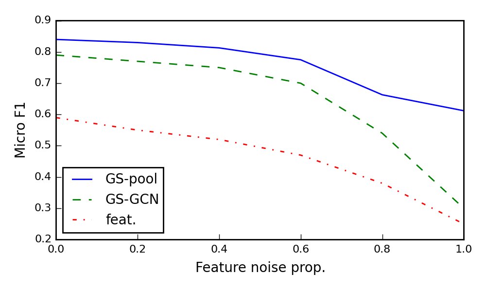
Figure 3: Accuracy (in F1-score) for different approaches on the citation data as the feature matrix is incrementally replaced with random Gaussian noise.
图 3:随着特征矩阵逐步被随机高斯噪声替换,不同方法在引文数据上的准确率(F1 分数)。
Finally, we note that Theorem 1 and Corollary 2 are expressed with respect to a particular given graph and are thus somewhat transductive. For the inductive setting, we can state
最后我们指出,定理 1 与推论 2 是针对给定的特定图表述的,因而多少带有直推色彩。对归纳设定,我们可以陈述
Corollary 3.
Suppose that for all graphs belonging to some class of graphs $G^{}\exists k,d\geq 0,k,d\in\mathbb{Z}$ such that*
推论 3。
假定对属于某类图 $G^{}\mathcal{G}=(\mathcal{V},\mathcal{E})k,d\geq 0k,d\in\mathbb{Z}$,使得*
then we can approximate clustering coefficients to an arbitrary epsilon after iterations of Algorithm .
则在算法 经 次迭代后,我们可以任意 精度逼近聚类系数。
Corollary 3 simply states that if after iterations of Algorithm 1, we can learn to uniquely identify nodes for a class of graphs, then we can also approximate clustering coefficients to an arbitrary precision for this class of graphs.
推论 3 简单地说:若算法 1 经 次迭代后,我们能学会为一类图唯一识别节点,则我们也能以任意精度逼近这类图的聚类系数。