GIRAFFE: Representing Scenes as Compositional Generative Neural Feature Fields

GIRAFFE：将场景表示为组合式生成神经特征场（GIRAFFE: Representing Scenes as Compositional Generative Neural Feature Fields）

Michael Niemeyer 1,2  Andreas Geiger 1,2 1 Max Planck Institute for Intelligent Systems    Tübingen    2 University of Tübingen {firstname.lastname}@tue.mpg.de

Michael Niemeyer¹˒² Andreas Geiger¹˒²
所属机构：¹Max Planck Institute for Intelligent Systems, Tübingen；²University of Tübingen
{firstname.lastname}@tue.mpg.de

Abstract

摘要

Deep generative models allow for photorealistic image synthesis at high resolutions. But for many applications, this is not enough: content creation also needs to be controllable. While several recent works investigate how to disentangle underlying factors of variation in the data, most of them operate in 2D and hence ignore that our world is three-dimensional. Further, only few works consider the compositional nature of scenes. Our key hypothesis is that incorporating a compositional 3D scene representation into the generative model leads to more controllable image synthesis. Representing scenes as compositional generative neural feature fields allows us to disentangle one or multiple objects from the background as well as individual objects’ shapes and appearances while learning from unstructured and unposed image collections without any additional supervision. Combining this scene representation with a neural rendering pipeline yields a fast and realistic image synthesis model. As evidenced by our experiments, our model is able to disentangle individual objects and allows for translating and rotating them in the scene as well as changing the camera pose.

深度生成模型已能在高分辨率下做照片级真实图像合成。但对许多应用这还不够：内容创作还需要可控。近来一些工作研究如何解耦数据中的潜在变化因素，但大多在 2D 操作，忽略了世界是三维的；考虑场景组合性的也很少。我们的核心假设是：把组合式 3D 场景表示纳入生成模型，能带来更可控的图像合成。把场景表示为「组合式生成神经特征场」，可在无额外监督的条件下，从未结构化、无位姿的图像集合中学习，把一个或多个物体与背景解耦，并分开物体形状与外观。将该场景表示与神经渲染管线结合，得到快速且真实的图像合成模型。实验表明，模型能解耦单个物体，支持在场景中平移、旋转物体并改变相机位姿。

1 Introduction

1 引言

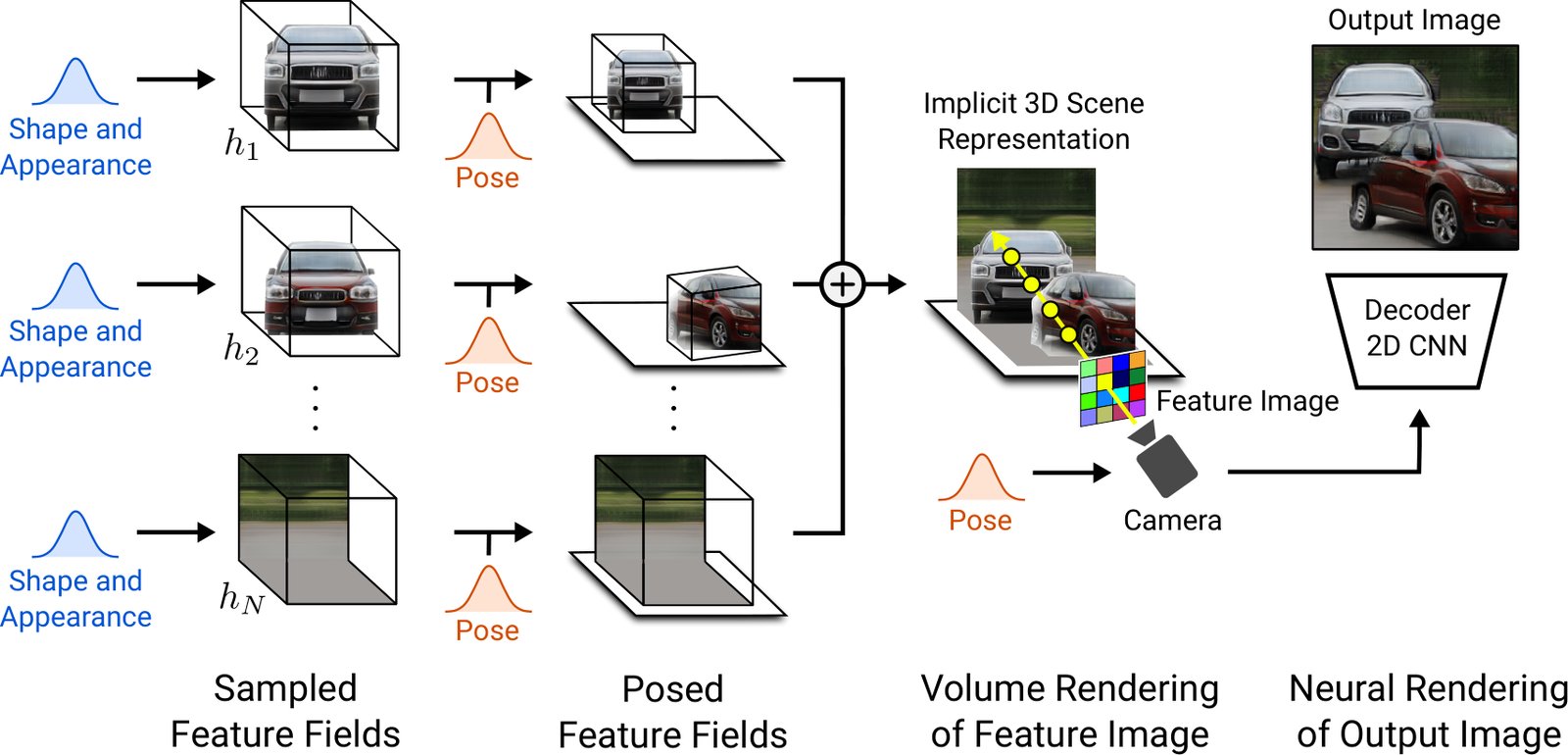
Figure 1: Overview. We represent scenes as compositional generative neural feature fields. For a randomly sampled camera, we volume render a feature image of the scene based on individual feature fields. A 2D neural rendering network converts the feature image into an RGB image. While training only on raw image collections, at test time we are able to control the image formation process wrt. camera pose, object poses, as well as the objects’ shapes and appearances. Further, our model generalizes beyond the training data, e.g. we can synthesize scenes with more objects than were present in the training images. Note that for clarity we visualize volumes in color instead of features.

图1:概览 我们代表场景作为组成基因神经特征领域. 对于随机采样的相机,我们量制成基于单个特征字段的场景特征图像. 一个2D神经渲染网络将特征图像转换成RGB图像. 虽然只培训原始图像集,但在测试时我们能够控制图像形成过程wrt. 相机姿势、物体姿势以及物体的形状和外观。 此外,我们的模型概括了训练数据以外的内容,例如,我们可以合成比训练图像中更多的物体的场景。 请注意,为了清晰起见,我们用颜色而不是特征来显示卷。

(a) Translation of Left Object (2D-based Method [71])

呵呵,左侧对象的翻译(2D方法[71])

The ability to generate and manipulate photorealistic image content is a long-standing goal of computer vision and graphics. Modern computer graphics techniques achieve impressive results and are industry standard in gaming and movie productions. However, they are very hardware expensive and require substantial human labor for 3D content creation and arrangement.

生成和操纵照片级真实主义图像内容的能力是计算机视觉和图形的长期目标. 现代计算机图形技术取得了令人印象深刻的成果,是游戏和电影制作的行业标准. 然而,它们非常昂贵的硬件,需要大量的人力来创造和安排3D内容.

In recent years, the computer vision community has made great strides towards highly-realistic image generation. In particular, Generative Adversarial Networks (GANs) [24] emerged as a powerful class of generative models. They are able to synthesize photorealistic images at resolutions of $1024^{2}$ pixels and beyond [39, 40, 14, 15, 6].

近年来,计算机视觉界在高度现实化的图像生成方面取得了长足的进步. 特别是Generative Adversarial Networks(GANs)[24]作为一个强大的生成模型类出现. 它们能够在$1024^{2}$像素的分辨率以及超过[39、40、14、15、6]的分辨率上合成照片级真实图像。

Despite these successes, synthesizing realistic 2D images is not the only aspect required in applications of generative models. The generation process should also be controllable in a simple and consistent manner. To this end, many works [9, 44, 71, 74, 39, 97, 43, 54, 48, 25, 98] investigate how disentangled representations can be learned from data without explicit supervision. Definitions of disentanglement vary [5, 53], but commonly refer to being able to control an attribute of interest, e.g. object shape, size, or pose, without changing other attributes. Most approaches, however, do not consider the compositional nature of scenes and operate in the 2D domain, ignoring that our world is three-dimensional. This often leads to entangled representations (\figreffig:controllable-generation) and control mechanisms are not built-in, but need to be discovered in the latent space a posteriori. These properties, however, are crucial for successful applications, e.g. a movie production where complex object trajectories need to be generated in a consistent manner.

尽管取得了这些成功,合成现实的2D图像并不是生成模型应用中唯一需要的方面. 生成过程也应以简单和一致的方式加以控制。 为此,许多著作[9,44,71,74,39,97,43,54,48,25,98]调查了如何在没有明确监督的情况下从数据中吸取分散的表述. 分散的定义各不相同[5,53],但通常是指能够控制某种利益属性,如物体形状,大小,或姿势,而不改变其他属性. 然而,大多数方法并不考虑场景的构成性质,而是在2D领域运作,忽略了我们的世界是三维的. 这经常导致缠绕的表示(\figreg:controlliable-generation),控制机制不是内置的,而需要在潜伏的空间中发现后置的. 然而,这些特性对于成功的应用至关重要,例如电影制作,其中复杂的物体轨迹需要以一致的方式产生.

Several recent works therefore investigate how to incorporate 3D representations, such as voxels [32, 63, 64], primitives [46], or radiance fields [77], directly into generative models. While these methods allow for impressive results with built-in control, they are mostly restricted to single-object scenes and results are less consistent for higher resolutions and more complex and realistic imagery (e.g. scenes with objects not in the center or cluttered backgrounds).

因此,最近的一些著作研究了如何将3D表示法,如葡萄酒[32,63,64],原始物[46],或辐射场[77]直接纳入生成模型. 虽然这些方法允许在内在控制下取得令人印象深刻的结果,但它们大多局限于单对象场景,对于更高的分辨率以及更复杂更现实的图像(例如有物体不在中心或背景杂乱的场景)来说,结果也不太一致.

Contribution: In this work, we introduce GIRAFFE, a novel method for generating scenes in a controllable and photorealistic manner while training from raw unstructured image collections. Our key insight is twofold: First, incorporating a compositional 3D scene representation directly into the generative model leads to more controllable image synthesis. Second, combining this explicit 3D representation with a neural rendering pipeline results in faster inference and more realistic images. To this end, we represent scenes as compositional generative neural feature fields (\figreffig:teaser). We volume render the scene to a feature image of relatively low resolution to save time and computation. A neural renderer processes these feature images and outputs the final renderings. This way, our approach achieves high-quality images and scales to real-world scenes. We find that our method allows for controllable image synthesis of single-object as well as multi-object scenes when trained on raw unstructured image collections. Code and data is available at https://github.com/autonomousvision/giraffe.

** 贡献**: 在这部作品中,我们引入GIFFE,这是一种新颖的方法,在从原始的无结构图像集训练的同时,以可控和照片级真实化的方式生成场景. 我们的关键见解是双重的:第一,将构成的3D场景表现直接纳入生成模型,导致更可控的图像合成. 其次,将这种明确的三维表示与神经渲染管道相结合,导致更快的推论和更加现实的图像. 为此,我们代表场景为组成基因神经特征场(\figrefigig:teaser). 为了节省时间和计算,我们量度使场景呈现出分辨率相对较低的特征图像。 神经渲染器处理这些特征图像并输出最终渲染. 这样,我们的方法就实现了高质量的图像和尺度到现实世界的场景. 我们发现,我们的方法允许在未经结构化的原始图像集上训练时,对单对象以及多对象场景进行可控图像合成. 代码和数据见https://github.com/aautomisticvision/giraffe。

2 Related Work

2 相关工作

GAN-based Image Synthesis: Generative Adversarial Networks (GANs) [24] have been shown to allow for photorealistic image synthesis at resolutions of $1024^{2}$ pixels and beyond [39, 40, 14, 15, 6]. To gain better control over the synthesis process, many works investigate how factors of variation can be disentangled without explicit supervision. They either modify the training objective [71, 40, 9] or network architecture [39], or investigate latent spaces of well-engineered and pre-trained generative models  [27, 16, 34, 78, 23, 1, 96]. All of these works, however, do not explicitly model the compositional nature of scenes. Recent works therefore investigate how the synthesis process can be controlled at the object-level [19, 90, 18, 4, 7, 26, 86, 3, 45]. While achieving photorealistic results, all aforementioned works model the image formation process in 2D, ignoring the three-dimensional structure of our world. In this work, we advocate to model the formation process directly in 3D for better disentanglement and more controllable synthesis.

基于GAN的图像合成: Generative Adversarial Networks (GANs) [24] 已被显示,在$1024^{2}$像素的分辨率以及超过[39, 40, 14, 15, 6] 的分辨率中允许照片级真实化图像合成. 为了更好地控制合成过程,许多著作都研究了如何在没有明确监督的情况下将变异因素分解. 它们要么修改培训目标[71、40、9]或网络架构[39],要么调查经过良好设计和预先培训的生成模型的潜在空间[27、16、34、78、23、1、96]。 然而,所有这些作品并没有明确地模拟场景的构成性质. 因此,近期的作品研究了如何在对象级控制合成过程[19,90,18,4,7,26,86,3,45]. 在取得照片级真实主义成果的同时,上述所有作品都以2D模拟图像形成过程,忽略了我们世界的三维结构. 在这项工作中,我们主张用3D直接模拟形成过程,以便更好地分解和更加可控的合成.

Implicit Functions: Using implicit functions to represent 3D geometry has gained popularity in learning-based 3D reconstruction [59, 69, 12, 67, 76, 65, 22, 11, 60] and has been extended to scene-level reconstruction [8, 35, 72, 79, 13]. To overcome the need of 3D supervision, several works [50, 66, 81, 92, 51] propose differentiable rendering techniques. Mildenhall et al. [61] propose Neural Radiance Fields (NeRFs) in which they combine an implicit neural model with volume rendering for novel view synthesis of complex scenes. Due to their expressiveness, we use a generative variant of NeRFs as our object-level representation. In contrast to our method, the discussed works require multi-view images with camera poses as supervision, train a single network per scene, and are not able to generate novel scenes. Instead, we learn a generative model from unstructured image collections which allows for controllable, photorealistic image synthesis of generated scenes.

** 隐式函数**: 使用隐含的函数来代表3D几何在基于学习的3D重建[59,69,12,67,76,65,22,11,60]中获得了欢迎,并被扩展至场景一级的重建[8,35,72,79,13]. 为了克服3D监理的需要,一些作品[50,66,81,92,51]提出了不同的渲染技术. Mildenhall等人[61]提出了神经辐射场(NERFs),其中他们将隐含的神经模型与体积渲染结合起来,用于对复杂场景进行新颖的视角合成. 由于它们的表达性,我们使用NERFs的生成变体作为我们的物体级代表. 与我们的方法不同,被讨论的作品需要多视图图像,并带有相机姿势作为监督,每个场景训练一个单一的网络,无法产生新奇的场景. 相反,我们从无结构的图像集中学习到一个生成模型,它允许对生成的场景进行可控的,照片级真实的图像合成.

3D-Aware Image Synthesis: Several works investigate how 3D representations can be incorporated as inductive bias into generative models [32, 55, 63, 64, 46, 77, 21, 75, 30, 31, 29]. While many approaches use additional supervision [99, 87, 2, 10, 88], we focus on works which are trained on raw image collections like our approach. Henzler et al. [32] learn voxel-based representations using differentiable rendering. The results are 3D controllable, but show artifacts due to the limited voxel resolutions caused by their cubic memory growth. Nguyen-Phuoc et al. [63, 64] propose voxelized feature-grid representations which are rendered to 2D via a reshaping operation. While achieving impressive results, training becomes less stable and results less consistent for higher resolutions. Liao et al. [46] use abstract features in combination with primitives and differentiable rendering. While handling multi-object scenes, they require additional supervision in the form of pure background images which are hard to obtain for real-world scenes. Schwarz et al. [77] propose Generative Neural Radiances Fields (GRAF). While achieving controllable image synthesis at high resolutions, this representation is restricted to single-object scenes and results degrade on more complex, real-world imagery. In contrast, we incorporate compositional 3D scene structure into the generative model such that it naturally handles multi-object scenes. Further, by integrating a neural rendering pipeline [20, 62, 81, 42, 49, 84, 83, 80, 41], our model scales to more complex, real-world data.

3D-Aware 图像合成: 若干作品研究了如何将3D表达法作为诱导偏差纳入生成模型[32,55,63,64,46,77,21,75,30,31,29]. 虽然许多方法都使用额外的监督[99、87、2、10、88],但我们侧重于像我们的方法那样在原始图像收集方面接受培训的作品。 Henzler et al. [32] 利用不同的渲染法来学习以 voxel 为基础的表达法. 结果为3D可控,但由于其立方内存生长引起的微分分辨率有限,故显示文物. Nguyen-Phuoc等人[63、64] 提出通过重塑操作制成2D的变形特征网表示。 在取得令人印象深刻的成果的同时,培训也变得不那么稳定,对更高决议而言,培训成果也不太一致。 廖等[46]使用抽象特征与原始物和异质渲染结合. 在处理多对象场景时,它们需要额外的监督,其形式是纯背景图像,对于现实世界的场景来说很难获得. 施瓦兹等人[77]提出基因神经辐射场(GRAF). 在高分辨率下实现可控图像合成的同时,这种表示仅限于单对象场景,结果在更为复杂,真实世界的图像上降解. 相比之下,我们把成分的3D场景结构纳入生成模型,这样它自然地处理多对象场景. 此外,通过整合神经渲染管道[20、62、81、42、49、84、83、80、41],我们的模型尺度将更复杂、更现实的数据。

3 Method

3 方法

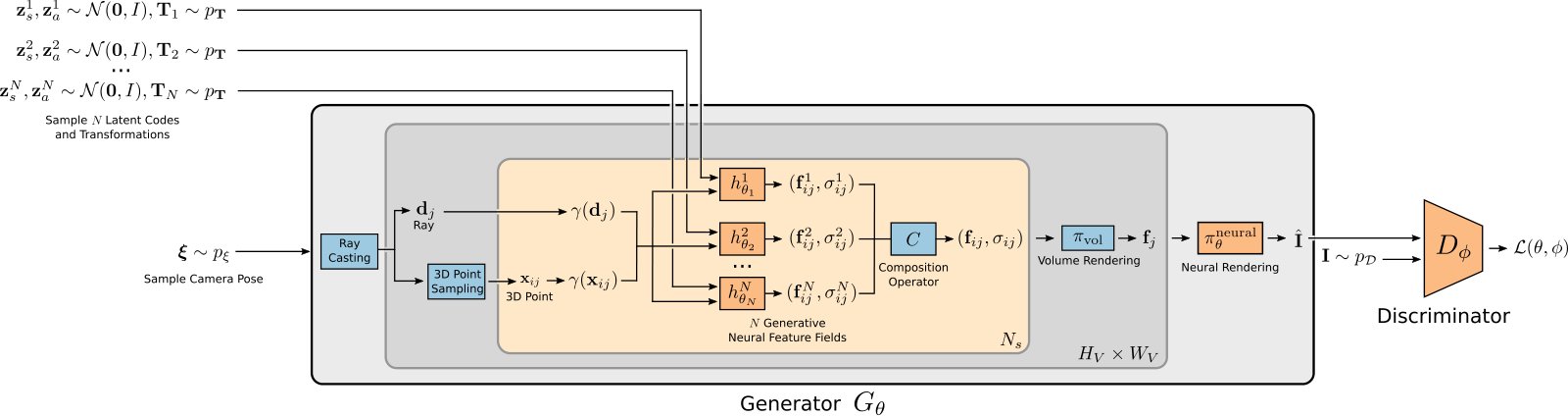
Figure 3: GIRAFFE. Our generator $G_{\theta}$ takes a camera pose $\boldsymbol{\xi}$ and $N$ shape and appearance codes $\mathbf{z}_{s}^{i},\mathbf{z}_{a}^{i}$ and affine transformations $\mathbf{T}_{i}$ as input and synthesizes an image of the generated scene which consists of $N-1$ objects and a background. The discriminator $D_{\phi}$ takes the generated image $\hat{\mathbf{I}}$ and the real image $\mathbf{I}$ as input and our full model is trained with an adversarial loss. At test time, we can control the camera pose, the shape and appearance codes of the objects, and the objects’ poses in the scene. Orange indicates learnable and blue non-learnable operations.

图3:全球森林研究基金 我们的发电机$G_{\theta}$采用照相机呈现$\boldsymbol{\xi}$和$N$的形状和外观代码 $\mathbf{z}_{s}^{i},\mathbf{z}_{a}^{i}$和affine变换 $\mathbf{T}_{i}$作为输入和合成生成场景的图像,由$N-1$物体和一个背景组成. 歧视者$D_{\phi}$将生成的图像$\hat{\mathbf{I}}$和真实的图像$\mathbf{I}$作为输入,我们的完整模型被训练成对抗性损失. 在测试时,我们可以控制相机的姿势、物体的形状和外观代码以及物体在现场的姿势。 橙色表示可学习和蓝色不可学习操作.

Our goal is a controllable image synthesis pipeline which can be trained from raw image collections without additional supervision. In the following, we discuss the main components of our method. First, we model individual objects as neural feature fields (\secrefsubsec:objects). Next, we exploit the additive property of feature fields to composite scenes from multiple individual objects (\secrefsubsec:scenes). For rendering, we explore an efficient combination of volume and neural rendering techniques (\secrefsubsec:rendering). Finally, we discuss how we train our model from raw image collections (\secrefsubsec:training). \figreffig:method-overview contains an overview of our method.

我们的目标是一个可控的图像合成管道,可以在没有额外监督的情况下从原始图像收集中培训。 下面我们讨论我们方法的主要组成部分。 首先,我们把单个物体模拟为神经特征域(\secrefsubsec:obobjects). 接下来,我们从多个单个物体(\secrefsubsec:scenes)中,将特征场的添加剂属性开发到复合场景. 对于渲染,我们探索将体积和神经渲染技术(\secrefsubsec:rendering)有效地结合起来. 最后,我们讨论如何从原始图像集(\secrefsubsec:training)中训练我们的模型. \figrefig:方法概览 包含了我们的方法。

3.1 Objects as Neural Feature Fields

3.1 物体作为神经特征场

Neural Radiance Fields: A radiance field is a continuous function $f$ which maps a 3D point $\mathbf{x}\in\mathbb{R}^{3}$ and a viewing direction $\mathbf{d}\in\mathbb{S}^{2}$ to a volume density $\sigma\in\mathbb{R}^{+}$ and an RGB color value $\mathbf{c}\in\mathbb{R}^{3}$. A key observation in [61, 82] is that the low dimensional input $\mathbf{x}$ and $\mathbf{d}$ needs to be mapped to higher-dimensional features to be able to represent complex signals when $f$ is parameterized with a neural network. More specifically, a pre-defined positional encoding is applied element-wise to each component of $\mathbf{x}$ and $\mathbf{d}$:

** 神经辐射场**: 辐射场是连续函数$f$,它将3D点$\mathbf{x}\in\mathbb{R}^{3}$和观察方向$\mathbf{d}\in\mathbb{S}^{2}$映射到体积密度$\sigma\in\mathbb{R}^{+}$和RGB色值$\mathbf{c}\in\mathbb{R}^{3}$. [61,82]中的一项关键观察是,低维输入$\mathbf{x}$和$\mathbf{d}$需要映射到更高维度的特性,以便在$f$被神经网络参数化时能够代表复杂的信号. 更具体地说,对$\mathbf{x}$和$\mathbf{d}$的每个组件都采用预先定义的位置编码:

$$\displaystyle\begin{split}\gamma(t,L)&=\
(\sin(2^{0}t\pi),&\cos(2^{0}t\pi),\dots,\sin(2^{L}t\pi),\cos(2^{L}t\pi))\end{split} \tag{1}$$

where $t$ is a scalar input, e.g. a component of $\mathbf{x}$ or $\mathbf{d}$, and $L$ the number of frequency octaves. In the context of generative models, we observe an additional benefit of this representation: It introduces an inductive bias to learn 3D shape representations in canonical orientations which otherwise would be arbitrary (see \figreffig:canonical-pose).

其中$t$是一个scalar输入,如$\mathbf{x}$或$\mathbf{d}$的一个组件,和$L$的频率八维数. 在生成模型方面,我们看到这种表述的另一个好处: 它引入了一种诱导性偏差,在规范朝向中学习3D形状的表示,否则会具有任意性(见\figraphig:canonical-pose).

Following implicit shape representations [59, 12, 69], Mildenhall et al. [61] propose to learn Neural Radiance Fields (NeRFs) by parameterizing $f$ with a multi-layer perceptron (MLP):

根据隐式表示 [59, 12, 69], Mildenhall 等人 [61] 建议通过参数化$f$以多层感知(MLP)来学习神经辐射场(NERFs):

$$\displaystyle\begin{split}f_{\theta}:\mathbb{R}^{L_{\mathbf{x}}}\times\mathbb{R}^{L_{\mathbf{d}}}&\to\mathbb{R}^{+}\times\mathbb{R}^{3}\
(\gamma(\mathbf{x}),\gamma(\mathbf{d}))&\mapsto(\sigma,\mathbf{c})\end{split} \tag{2}$$

where $\theta$ indicate the network parameters and $L_{\mathbf{x}},L_{\mathbf{d}}$ the output dimensionalities of the positional encodings.

其中$\theta$表示网络参数,$L_{\mathbf{x}},L_{\mathbf{d}}$表示位置编码的输出维度.

Generative Neural Feature Fields: While [61] fits $\theta$ to multiple posed images of a single scene, Schwarz et al. [77] propose a generative model for Neural Radiance Fields (GRAF) that is trained from unposed image collections. To learn a latent space of NeRFs, they condition the MLP on shape and appearance codes $\mathbf{z}_{s},\mathbf{z}_{a}\sim\mathcal{N}(\mathbf{0},I)$:

** Generative Neural Feature Fields**: 虽然[61]适合$\theta$对一个单一场景的多个摆放图像,但Schwarz等人[77]为神经放射场(GRAF)提出了一个生成模型,该模型是从未放置图像集中训练出来的. 为了了解NERFs的潜在空间,它们将MLP以形状和外观代码$\mathbf{z}_{s},\mathbf{z}_{a}\sim\mathcal{N}(\mathbf{0},I)$作为条件:

$$\displaystyle\begin{split}g_{\theta}:\mathbb{R}^{L_{\mathbf{x}}}\times\mathbb{R}^{L_{\mathbf{d}}}\times\mathbb{R}^{M_{s}}\times\mathbb{R}^{M_{a}}&\to\mathbb{R}^{+}\times\mathbb{R}^{3}\
(\gamma(\mathbf{x}),\gamma(\mathbf{d}),\mathbf{z}{s},\mathbf{z}{a})&\mapsto(\sigma,\mathbf{c})\end{split} \tag{3}$$

where $M_{s},M_{a}$ are the dimensionalities of the latent codes.

其中$M_{s},M_{a}$是潜在代码的维度。

In this work we explore a more efficient combination of volume and neural rendering. We replace GRAF’s formulation for the three-dimensional color output $\mathbf{c}$ with a more generic $M_{f}$-dimensional feature $\mathbf{f}$ and represent objects as Generative Neural Feature Fields:

在这项工作中,我们探索了更高效地结合体积和神经渲染. 我们用更通用的$M_{f}$- 维特性$\mathbf{f}$取代 GRAF 用于三维色输出$\mathbf{c}$的配体, 并代表物体为 Generative Neural Feature Fields:

$$\displaystyle\begin{split}h_{\theta}:\mathbb{R}^{L_{\mathbf{x}}}\times\mathbb{R}^{L_{\mathbf{d}}}\times\mathbb{R}^{M_{s}}\times\mathbb{R}^{M_{a}}&\to\mathbb{R}^{+}\times\mathbb{R}^{M_{f}}\
(\gamma(\mathbf{x}),\gamma(\mathbf{d}),\mathbf{z}{s},\mathbf{z}{a})&\mapsto(\sigma,\mathbf{f})\end{split} \tag{4}$$

Object Representation: A key limitation of NeRF and GRAF is that the entire scene is represented by a single model. As we are interested in disentangling different entities in the scene, we need control over the pose, shape and appearance of individual objects (we consider the background as an object as well). We therefore represent each object using a separate feature field in combination with an affine transformation

** 目标代表**: NERF和GRAF的一个关键限制是整个场景由单一模型代表. 由于我们有兴趣将现场的不同实体分开,我们需要对 * 个人* 物体的姿势、形状和外观进行控制(我们也把背景视为物体)。 因此,我们用一个单独的特征字段,结合affine变换来代表每个对象

$$\displaystyle\begin{split}\mathbf{T}=\{\mathbf{s},\mathbf{t},\mathbf{R}\}\end{split} \tag{5}$$

where $\mathbf{s},\mathbf{t}\in\mathbb{R}^{3}$ indicate scale and translation parameters, and $\mathbf{R}\in SO(3)$ a rotation matrix. Using this representation, we transform points from object to scene space as follows:

其中$\mathbf{s},\mathbf{t}\in\mathbb{R}^{3}$表示尺度和翻译参数,$\mathbf{R}\in SO(3)$表示旋转矩阵. 利用这种表示方式,我们把点从物体转变为场景空间如下:

$$\displaystyle\begin{split}k(\mathbf{x})=\mathbf{R}\cdot\begin{bmatrix}s_{1}&&\
&s_{2}&\
&&s_{3}\end{bmatrix}\cdot\mathbf{x}+\mathbf{t}\end{split} \tag{6}$$

In practice, we volume render in scene space and evaluate the feature field in its canonical object space (see \figreffig:teaser):

在实际操作中,我们在场景空间进行体积渲染,并评价其犬形物体空间的特征场(见\figraffig:teaser):

$$\displaystyle\begin{split}(\sigma,\mathbf{f})=h_{\theta}(\gamma(k^{-1}(\mathbf{x})),\gamma(k^{-1}(\mathbf{d})),\mathbf{z}_{s},\mathbf{z}_{a})\end{split} \tag{7}$$

This allows us to arrange multiple objects in a scene. All object feature fields share their weights and $\mathbf{T}$ is sampled from a dataset-dependent distribution (see \secrefsubsec:training).

这样我们就可以在一幕中安排多个物体. 所有对象特征字段共享其权重,$\mathbf{T}$从一个依赖数据集的分布(见\secrefsubsec:training)中取样.

3.2 Scene Compositions

3.2 场景组合

As discussed above, we describe scenes as compositions of $N$ entities where the first $N-1$ are the objects in the scene and the last represents the background. We consider two cases: First, $N$ is fixed across the dataset such that the images always contain $N-1$ objects plus the background. Second, $N$ is varied across the dataset. In practice, we use the same representation for the background as for objects except that we fix the scale and translation parameters $\mathbf{s}_{N},\mathbf{t}_{N}$ to span the entire scene, and to be centered at the scene space origin.

如上所述,我们将场景描述为$N$实体的构成,其中第一个$N-1$是场景中的物体,最后一个代表背景. 我们考虑两种情况:第一,$N$固定在数据集之间,这样图像总是包含$N-1$对象加上背景. 第二,$N$因数据集而异。 在实际操作中,我们对背景使用与物体相同的表示,除了我们固定尺度和翻译参数$\mathbf{s}_{N},\mathbf{t}_{N}$,以覆盖整个场景,并以场景空间源为中心.

Composition Operator: To define the composition operator $C$, let’s recall that a feature field of a single entity $h_{\theta_{i}}^{i}$ predicts a density $\sigma_{i}\in\mathbb{R}^{+}$ and a feature vector $\mathbf{f}_{i}\in\mathbb{R}^{M_{f}}$ for a given point $\mathbf{x}$ and viewing direction $\mathbf{d}$. When combining non-solid objects, a natural choice [17] for the overall density at $\mathbf{x}$ is to sum up the individual densities and to use the density-weighted mean to combine all features at $(\mathbf{x},\mathbf{d})$:

** 组合运算符**: 为了定义组成操作员$C$,让我们回顾,一个单一实体$h_{\theta_{i}}^{i}$的特征字段预测密度$\sigma_{i}\in\mathbb{R}^{+}$和特定点$\mathbf{x}$的特征矢量$\mathbf{f}_{i}\in\mathbb{R}^{M_{f}}$,以及观察方向$\mathbf{d}$。 在结合非固体物体时,对$\mathbf{x}$的整体密度进行自然选择[17]是汇总单个密度,并使用密度加权平均值结合$(\mathbf{x},\mathbf{d})$的所有特征:

$$\displaystyle\begin{split}C(\mathbf{x},\mathbf{d})=\left(\sigma,\frac{1}{\sigma}\sum_{i=1}^{N}\sigma_{i}\mathbf{f}_{i}\right)\text{, where}\quad\sigma=\sum_{i=1}^{N}\sigma_{i}\end{split} \tag{8}$$

While being simple and intuitive, this choice for $C$ has an additional benefit: We ensure gradient flow to all entities with a density greater than $0$.

在简单和直观的同时,对$C$的这一选择还有一个好处: 我们确保梯度流向密度大于$0$的所有实体。

3.3 Scene Rendering

3.3 场景渲染

3D Volume Rendering: While previous works [61, 77, 47, 57] volume render an RGB color value, we extend this formulation to rendering an $M_{f}$-dimensional feature vector $\mathbf{f}$.

3D 体积渲染: 虽然以前的作品[61,77,47,57]体积生成了RGB的色彩值,但我们将这种配方扩展为渲染$M_{f}$ -维度特征矢量$\mathbf{f}$.

For given camera extrinsics $\boldsymbol{\xi}$, let $\{\mathbf{x}_{j}\}_{j=1}^{N_{s}}$ be sample points along the camera ray $\mathbf{d}$ for a given pixel, and $(\sigma_{j},\mathbf{f}_{j})=C(\mathbf{x}_{j},\mathbf{d})$ the corresponding densities and feature vectors of the field. The volume rendering operator $\pi_{\text{vol}}$ [37] maps these evaluations to the pixel’s final feature vector $\mathbf{f}$:

对于给定的相机外观 $\boldsymbol{\xi}$,让$\{\mathbf{x}_{j}\}_{j=1}^{N_{s}}$作为相机射线 $\mathbf{d}$的样本点用于给定的像素,让$(\sigma_{j},\mathbf{f}_{j})=C(\mathbf{x}_{j},\mathbf{d})$作为相应的密度和场的特征矢量. 量渲染操作员$\pi_{\text{vol}}$ [37]将这些评价映射到像素的最终特性矢量$\mathbf{f}$:

$$\displaystyle\begin{split}\pi_{\text{vol}}:(\mathbb{R}^{+}\times\mathbb{R}^{M_{f}})^{N_{s}}\to\mathbb{R}^{M_{f}},\quad\{\sigma_{j},\mathbf{f}_{j}\}_{j=1}^{N_{s}}\mapsto\mathbf{f}\end{split} \tag{9}$$

Using numerical integration as in [61], $\mathbf{f}$ is obtained as

使用[61]中的数字集成法,$\mathbf{f}$作为

$$\displaystyle\begin{split}\mathbf{f}=\sum_{j=1}^{N_{s}}\tau_{j}\alpha_{j}\mathbf{f}_{j}\quad\tau_{j}=\prod_{k=1}^{j-1}(1-\alpha_{k})\quad\alpha_{j}=1-e^{-\sigma_{j}\delta_{j}}\end{split} \tag{10}$$

where $\tau_{j}$ is the transmittance, $\alpha_{j}$ the alpha value for $\mathbf{x}_{j}$, and $\delta_{j}={\left|\left|\mathbf{x}_{j+1}-\mathbf{x}_{j}\right|\right|}_{2}$ the distance between neighboring sample points. The entire feature image is obtained by evaluating $\pi_{\text{vol}}$ at every pixel. For efficiency, we render feature images at resolution $16^{2}$ which is lower than the output resolution of $64^{2}$ or $256^{2}$ pixels. We then upsample the low-resolution feature maps to higher-resolution RGB images using 2D neural rendering. As evidenced by our experiments, this has two advantages: increased rendering speed and improved image quality.

其中$\tau_{j}$为传输值,$\alpha_{j}$为$\mathbf{x}_{j}$的α值,$\delta_{j}={\left|\left|\mathbf{x}_{j+1}-\mathbf{x}_{j}\right|\right|}_{2}$为相邻样本点之间的距离. 整个特征图像是通过在每个像素上评价$\pi_{\text{vol}}$而获得的. 为了提高效率,我们在第$16^{2}$号决议中渲染特性图像,它低于第$64^{2}$或第$256^{2}$像素的输出分辨率。 然后我们用2D神经渲染法把低分辨率特征图 提升到更高分辨率的RGB图像。 正如我们的实验所证明的,这有两个优点:增加渲染速度和改善图像质量.

2D Neural Rendering:

2D 神经渲染:

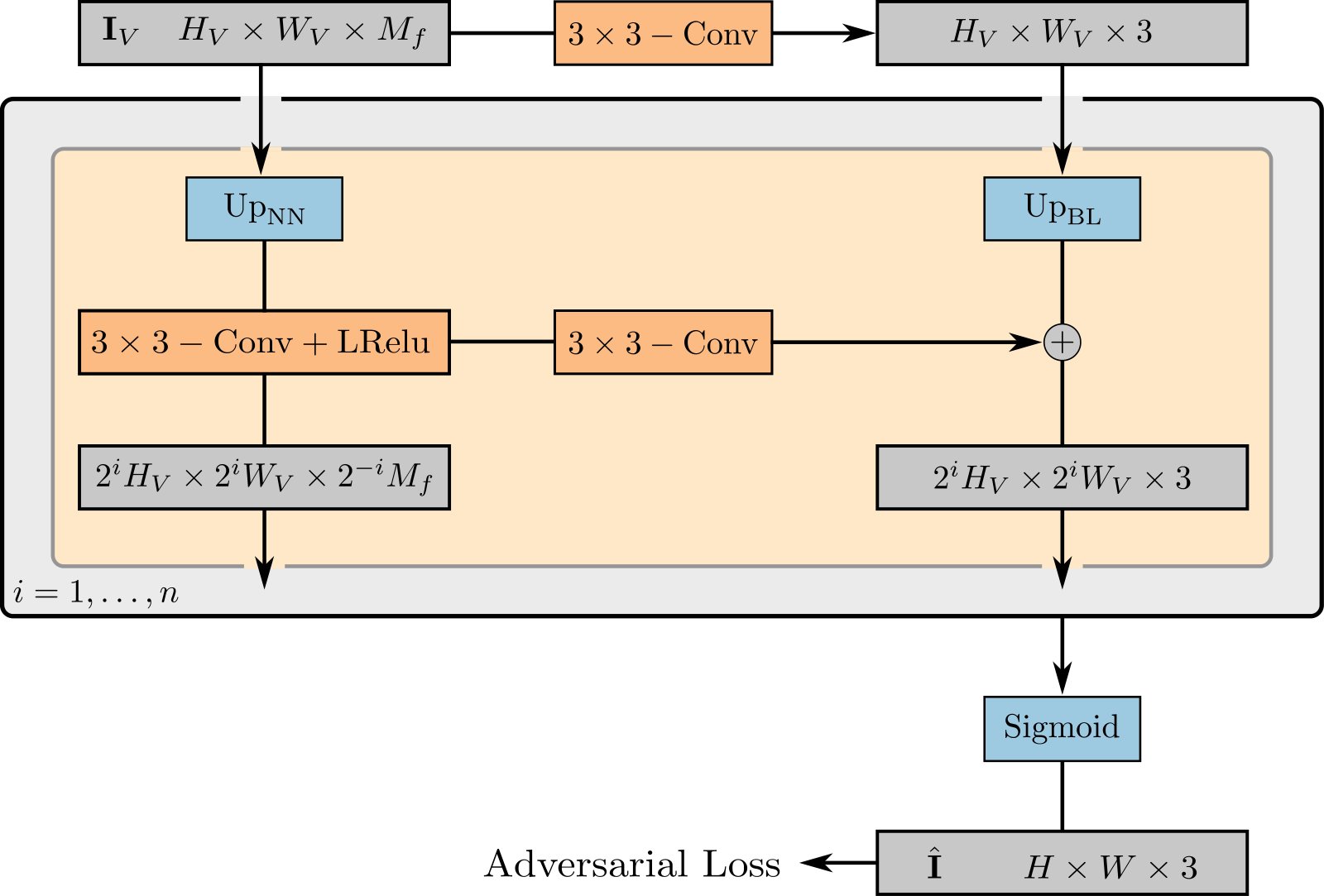
Figure 4: Neural Rendering Operator. The feature image $\mathbf{I}_{V}$ is processed by $n$ blocks of nearest neighbor upsampling and $3\times 3$ convolutions with leaky ReLU activations. At every resolution, we map the feature image to an RGB image with a $3\times 3$ convolution and add it to the previous output via bilinear upsampling. We apply a sigmoid activation to obtain the final image $\hat{\mathbf{I}}$. Gray color indicates outputs, orange learnable, and blue non-learnable operations.

图4:**神经渲染操作员。 ** 特征图像$\mathbf{I}_{V}$由最近邻居的$n$区块进行处理, 和$3\times 3$演化与漏流 ReLU 激活. 在每个分辨率上,我们用$3\times 3$的演化图谱将特征图像映射到一个RGB图像,并通过双线性升标法将其添加到之前的输出中. 我们使用 sigmoid 激活来获取最终图像$\hat{\mathbf{I}}$。 灰色颜色表示输出,橙色可学习,蓝色不可学习操作.

The neural rendering operator

神经渲染操作员

$$\displaystyle\begin{split}\pi_{\theta}^{\text{neural}}:\mathbb{R}^{H_{V}\times W_{V}\times M_{f}}\to\mathbb{R}^{H\times W\times 3}\end{split} \tag{11}$$

with weights $\theta$ maps the feature image $\mathbf{I}_{V}\in\mathbb{R}^{H_{V}\times W_{V}\times M_{f}}$ to the final synthesized image $\hat{\mathbf{I}}\in\mathbb{R}^{H\times W\times 3}$. We parameterize $\pi_{\theta}^{\text{neural}}$ as a 2D convolutional neural network (CNN) with leaky ReLU [89, 56] activation (\figreffig:neural-rendering) and combine nearest neighbor upsampling with $3\times 3$ convolutions to increase the spatial resolution. We choose small kernel sizes and no intermediate layers to only allow for spatially small refinements to avoid entangling global scene properties during image synthesis while at the same time allowing for increased output resolutions. Inspired by [40], we map the feature image to an RGB image at every spatial resolution, and add the previous output to the next via bilinear upsampling. These skip connections ensure a strong gradient flow to the feature fields. We obtain our final image prediction $\hat{\mathbf{I}}$ by applying a sigmoid activation to the last RGB layer. We validate our design choices in an ablation study (\tabreftab:ablation-study).

带有权重的$\theta$将特征图像$\mathbf{I}_{V}\in\mathbb{R}^{H_{V}\times W_{V}\times M_{f}}$映射到最终合成的图像$\hat{\mathbf{I}}\in\mathbb{R}^{H\times W\times 3}$. 将$\pi_{\theta}^{\text{neural}}$参数化为2D的转录神经 của了漏流的ReLU[89,56]激活(\figrefigg:neural-rendering),并将最近的邻上采样与$3\times 3$的转录结合,以增加空间分辨率. 我们选择小内核大小和没有中间层,只允许空间小的改进,以避免在图像合成过程中将全局场景属性包裹在一起,同时允许增加输出分辨率. 在[40]的启发下,我们将特性图像映射到每个空间分辨率的 RGB 图像,并通过双线性提升样本将之前的输出添加到下一个. 这些跳过连接确保了强大的梯度流到特性字段. 我们通过在最后一个RGB层上应用Sigmoid激活来获得我们的最终图像预测$\hat{\mathbf{I}}$. 我们在一项研究中验证我们的设计选择(\tabreftab:ablation-study).

3.4 Training

3.4 训练

Generator: We denote the full generative process formally as

** 发电机**: 我们正式表示完整的基因过程是

$$\displaystyle\begin{split}G_{\theta}({\mathbf{z}{s}^{i},\mathbf{z}{a}^{i},\mathbf{T}{i}}{i=1}^{N},\boldsymbol{\xi})=\pi_{\theta}^{\text{neural}}(\mathbf{I}{V})&\
\text{where}\quad\mathbf{I}{V}={\pi_{\text{vol}}({C(\mathbf{x}{jk},\mathbf{d}{k})}{j=1}^{N{s}})&}{k=1}^{H{V}\times W_{V}}\end{split} \tag{12}$$

and $N$ is the number of entities in the scene, $N_{s}$ the number of sample points along each ray, $\mathbf{d}_{k}$ is the ray for the $k$-th pixel, and $\mathbf{x}_{jk}$ the $j$-th sample point for the $k$-th pixel / ray.

而$N$是场景中的实体数,$N_{s}$是沿每条射线的样本点数,$\mathbf{d}_{k}$是$k$ - 第十一像素的射线,$\mathbf{x}_{jk}$是$j$ - 第十一像素/射线的样本点.

Discriminator: We parameterize the discriminator $D_{\phi}$ as a CNN [73] with leaky ReLU activation.

** 歧视者**: 我们把歧视者$D_{\phi}$作为CNN [73] 的参数, 以泄露的ReLU激活.

Training: During training, we sample the the number of entities in the scene $N\sim p_{N}$, the latent codes $\mathbf{z}_{s}^{i},\mathbf{z}_{a}^{i}\sim\mathcal{N}(\mathbf{0},I)$, as well as a camera pose $\boldsymbol{\xi}\sim p_{\xi}$ and object-level transformations $\mathbf{T}_{i}\sim p_{T}$. In practice, we define $p_{\xi}$ and $p_{T}$ as uniform distributions over dataset-dependent camera elevation angles and valid object transformations, respectively.[^1] The motivation for this choice is that in most real-world scenes, objects are arbitrarily rotated, but not tilted due to gravity. The observer (the camera in our case), in contrast, can freely change its elevation angle wrt. the scene.

** 培训**: 在培训期间,我们抽样了场景$N\sim p_{N}$中的实体数量,潜伏代码$\mathbf{z}_{s}^{i},\mathbf{z}_{a}^{i}\sim\mathcal{N}(\mathbf{0},I)$,以及一台照相机呈现$\boldsymbol{\xi}\sim p_{\xi}$和物体级转换的$\mathbf{T}_{i}\sim p_{T}$. 在实践中,我们将$p_{\xi}$和$p_{T}$分别定义为数据集依赖的相机高角和有效对象转换上的统一分布. [^1] 这种选择的动机是,在大多数现实世界的场景中,物体会任意旋转,但不会因为重力而倾斜. 相对而言,观察者(我们的摄影机)可以自由改变其仰角。 现场。

We train our model with the non-saturating GAN objective [24] and $R_{1}$ gradient penalty [58]

我们用不饱和GAN目标[24]和$R_{1}$梯度罚[58]来训练我们的模型.

$$\begin{split}&\mathcal{V}(\theta,\phi)=\
&\mathbb{E}{\mathbf{z}{s}^{i},\mathbf{z}{a}^{i}\sim\mathcal{N},,\boldsymbol{\xi}\sim p{\xi},,\mathbf{T}{i}\sim p{T}}\left[f(D_{\phi}(G_{\theta}({\mathbf{z}{s}^{i},\mathbf{z}{a}^{i},\mathbf{T}{i}}{i},\boldsymbol{\xi}))\right]\
&+\mathbb{E}{\mathbf{I}\sim p{\mathcal{D}}}\left[f(-D_{\phi}(\mathbf{I}))-,\lambda{|\nabla D_{\phi}(\mathbf{I})|}^{2}\right]\end{split} \tag{13}$$

where $f(t)=-\log(1+\exp(-t))$, $\lambda=10$, and $p_{\mathcal{D}}$ indicates the data distribution.

其中$f(t)=-\log(1+\exp(-t))$、$\lambda=10$和$p_{\mathcal{D}}$表示数据分布情况。

3.5 Implementation Details

3.5 实现细节

All object feature fields $\{h_{\theta_{i}}^{i}\}_{i=1}^{N-1}$ share their weights and we parametrize them as MLPs with ReLU activations. We use $8$ layers with a hidden dimension of $128$ and a density and a feature head of dimensionality $1$ and $M_{f}=128$, respectively. For the background feature field $h_{\theta_{N}}^{N}$, we use half the layers and hidden dimension. We use $L_{\mathbf{x}}=2\cdot 3\cdot 10$ and $L_{\mathbf{d}}=2\cdot 3\cdot 4$ for the positional encodings. We sample $M_{s}=64$ points along each ray and render the feature image $\mathbf{I}_{V}$ at $16^{2}$ pixels. We use an exponential moving average [93] with decay $0.999$ for the weights of the generator. We use the RMSprop optimizer [85] with a batch size of $32$ and learning rates of $1\text{\times}{10}^{-4}$ and $5\text{\times}{10}^{-4}$ for the discriminator and generator, respectively. For experiments at $256^{2}$ pixels, we set $M_{f}=256$ and half the generator learning rate to $2.5\text{\times}{10}^{-4}$.

所有物体特征字段$\{h_{\theta_{i}}^{i}\}_{i=1}^{N-1}$都分享它们的重量,我们用ReLU激活来将它们作为MLP进行偏移. 我们使用$8$层,其隐藏维度分别为$128$,密度和维度的特征头分别为$1$和$M_{f}=128$. 对于背景特征字段$h_{\theta_{N}}^{N}$,我们使用半层和隐藏维度. 我们使用$L_{\mathbf{x}}=2\cdot 3\cdot 10$和$L_{\mathbf{d}}=2\cdot 3\cdot 4$进行位置编码. 我们沿着每条射线对$M_{s}=64$点进行取样,并在$16^{2}$像素上渲染出特征图像$\mathbf{I}_{V}$. 我们使用指数移动平均值[93] 和衰变的$0.999$来表示发电机的重量。 我们使用RMSprop优化器[85],批量尺寸为$32$,对歧视者和生成者分别使用$1\text{\times}{10}^{-4}$和$5\text{\times}{10}^{-4}$的学习率. 对于$256^{2}$像素的实验,我们设定了$M_{f}=256$和发电机学习率的一半到$2.5\text{\times}{10}^{-4}$.

4 Experiments

4 实验

Datasets: We report results on commonly-used single-object datasets Chairs [68], Cats [95], CelebA [52], and CelebA-HQ [38]. The first consists of synthetic renderings of Photoshape chairs [70], and the others are image collections of cat and human faces, respectively. The data complexity is limited as the background is purely white or only takes up a small part of the image. We further report results on the more challenging single-object, real-world datasets CompCars [91], LSUN Churches [94], and FFHQ [39]. For CompCars, we randomly crop the images to achieve more variety of the object’s position in the image.[^2] For these datasets, disentangling objects is more complex as the object is not always in the center and the background is more cluttered and takes up a larger part of the image. To test our model on multi-object scenes, we use the script from [36] to render scenes with $2$, $3$, $4$, or $5$ random primitives (Clevr-N). To test our model on scenes with a varying number of objects, we also run our model on the union of them (Clevr-2345).

** 任务**: 我们报告常用的单对象数据集结果 * 主席* [68]、卡特 [95]、凯莱布 [52] 和凯莱布-HQ[38]。 第一种是合成的Photoshape椅渲染[70],其他分别是猫和人脸的图像集. 数据复杂性有限,因为背景纯粹是白色的,或者只占图像的一小部分. 我们进一步报告对单一对象、现实世界数据集更具挑战性的结果。 对于*CompCars *,我们随机裁剪图像,以在图像中实现对象位置的更多多样性. [^2] 对于这些数据集来说,脱落对象比较复杂,因为对象并不总是位于中心,背景较为杂乱,占据了图像的较大部分. 为了在多对象场景上测试我们的模型,我们使用来自[36] 的脚本,用$2$,$3$,$4$,或$5$随机原始(Clevr-N)来渲染场景. 为了用不同数量的物体在场景上测试我们的模型,我们还在它们的结合上运行我们的模型(Clevr-2345).

Baselines: We compare against voxel-based PlatonicGAN [32], BlockGAN [64], and HoloGAN [63], and radiance field-based GRAF [77] (see \secrefsec:rel-work for a discussion of the methods). We further compare against HoloGAN w/o 3D Conv, a variant of [63] proposed in [77] for higher resolutions. We additionally report a ResNet-based [28] 2D GAN [58] for reference.

** 巴塞尔**: 我们比较了Voxel基PlatonicGAN[32],BlockGAN[64]和HoloGAN[63],以及辐射基GRAF77。 我们还比较了HoloGAN w/o 3D Conv,这是[77]中为更高分辨率提议的[63]的变体。 我们还要报告一个基于ResNet的[28] 2D GAN[58],以供参考。

Metrics: We report the Frechet Inception Distance (FID) score [33] to quantify image quality. We use $20true000$ real and fake samples to calculate the FID score.

** 计量**: 我们报告Frechet受体距离(FID)分数[33],以量化图像质量。 我们使用$20true000$真假样本计算FID分数.

4.1 Controllable Scene Generation

4.1 可控场景生成

Chairs	CelebA	Churches	Cars	Clevr-5	Clevr-2345

Figure 5: Scene Disentanglement. From top to bottom, we show only backgrounds, only objects, color-coded object alpha maps, and the final synthesized images at $64^{2}$ pixel resolution. Disentanglement emerges without supervision, and the model learns to generate plausible backgrounds although the training data only contains images with objects.

主席	塞莱巴	教会	汽车	列车5型	列车2345

图5:** 场景分裂。 ** 从上到下,我们只显示背景,只显示对象,色码对象α地图,最后合成的图像在$64^{2}$像素分辨率. 虽然训练数据中只包含带有物体的图像,但分离现象在没有监督的情况下出现,模型学习产生可信的背景.

Figure 6: Training Progression. We show renderings of our model on Clevr-2345 at $256^{2}$ pixels after $0$, $1$, $2$, $3$, $10$, and $100$-thousand iterations. Unsupervised disentanglement emerges already at the very beginning of training.

图6:**培训进展。 ** 我们在 $0$, $1$, $2$, $3$, $10$, 和$100$- 千倍重迭之后的$256^{2}$像素上显示我们的模型的渲染。 在训练之初就已经出现了不受监督的分散现象。

(a) Object Rotation

(a) 物体旋转

(a) Increase Depth Translation

(a) 增加深度翻译

Disentangled Scene Generation: We first analyze to which degree our model learns to generate disentangled scene representations. In particular, we are interested if objects are disentangled from the background. Towards this goal, we exploit the fact that our composition operator is a simple addition operation (Eq. 8) and render individual components and object alpha maps (Eq. 10). Note that while we always render the feature image at $16^{2}$ during training, we can choose arbitrary resolutions at test time.

** 分散的场景**: 我们首先分析我们的模型 在多大程度上学会产生分散的场景表现。 特别是,如果物体与背景脱节,我们感兴趣。 为了实现这一目标,我们利用我们的构成操作员是一个简单的添加操作(Eq.8),并生成单个组件和对象α图(Eq.10)这一事实. 请注意,虽然我们在训练期间总是在$16^{2}$制作特性图像,但可以在测试时选择任意分辨率.

fig:disentanglement suggests that our method disentangles objects from the background. Note that this disentanglement emerges without any supervision, and the model learns to generate plausible backgrounds without ever having seen a pure background image, implicitly solving an inpainting task. We further observe that our model correctly disentangles individual objects when trained on multi-object scenes with fixed or varying number of objects. We further find that unsupervised disentanglement is a property of our model which emerges already at the very beginning of training (\figreffig:training-progression). Note how our model synthesizes individual objects before spending capacity on representing the background.

fig: 分散表示我们的方法将对象从背景中分离。 请注意,这种脱节现象在没有监督的情况下出现,模型学会产生可信的背景,而从未见过纯背景图像,暗含地解决了一种涂抹任务. 我们进一步观察到,我们的模型在用固定或不同数目的物体对多物体场景进行训练时,正确地使单个物体脱落。 我们进一步发现,不受监督的分离是我们模式的一个财产,它已经在培训之初出现(\figraphig: training-Progression)。 注意我们的模型如何在花费能力来代表背景之前合成单个对象.

Controllable Scene Generation: As individual components of the scene are correctly disentangled, we analyze how well they can be controlled. More specifically, we are interested if individual objects can be rotated and translated, but also how well shape and appearance can be controlled. In \figreffig:controllable-scene-gen, we show examples in which we control the scene during image synthesis. We rotate individual objects, translate them in 3D space, or change the camera elevation. By modeling shape and appearance for each entity with a different latent code, we are further able to change the objects’ appearances without altering their shape.

** 可控制场景生成**: 随着场景的单个部分被正确分解,我们分析它们能在多大程度上得到控制. 更具体地说,我们有兴趣的是单个物体能否被旋转和翻译,但也可以控制形状和外观。 在\figreffig:可控-scene-gen中,我们展示了在图像合成过程中控制场景的例子. 我们旋转单个物体,用3D空间翻译,或者改变相机高度. 通过给每个具有不同潜在代码的实体建模形状和外观,我们进一步能够改变物体的外观,而不改变其形状。

Generalization Beyond Training Data: The learned compositional scene representations allow us to generalize outside the training distribution. For example, we can increase the translation ranges of objects or add more objects than there were present in the training data (\figreffig:generalization).

** 培训之外的一般化数据**: 学习到的构成场景表现使我们能够在培训分配之外进行概括。 例如,我们可以增加对象的翻译范围,或者添加比训练数据(\figreffig:generalization)中存在的更多的对象.

4.2 Comparison to Baseline Methods

4.2 与基线方法比较

	Cats	CelebA	Cars	Chairs	Churches
2D GAN [58]	18	15	16	59	19
Plat. GAN [32]	318	321	299	199	242
BlockGAN [64]	47	69	41	41	28
HoloGAN [63]	27	25	17	59	31
GRAF [77]	26	25	39	34	38
Ours	8	6	16	20	17

Table 1: Quantitative Comparison. We report the FID score ($\downarrow$) at $64^{2}$ pixels for baselines and our method.

	猫	塞莱巴	与各国的汽车	主席	教会
2D GAN [58] (英语).	18	15	页:1	59	19
Plat. GAN [32] (英语).	318	321	299	199	242
块GAN [64]	47	69	41	41	28
霍洛甘 [63]	27	25	17	59	31
GRAF [77] (法语).	26	25	39	34	38
我们的	** 本文件迟交,是因为需要翻译。	页:1	页:1	页:1	页:1

表1:定量比较。 ** 我们以$64^{2}$像素报告FID得分($\downarrow$),用于基线和我们的方法。

	CelebA-HQ	FFHQ	Cars	Churches	Clevr-2
HoloGAN [63]	61	192	34	58	241
w/o 3D Conv	33	70	49	66	273
GRAF [77]	49	59	95	87	106
Ours	21	32	26	30	31

Table 2: Quantitative Comparison. We report the FID score ($\downarrow$) at $256^{2}$ pixels for the strongest 3D-aware baselines and our method.

	塞莱巴总部	总部	汽车	教会	lev二.
霍洛甘 [63]	61	192	34	58	241
3D 协议	33	70	49	66	273
GRAF [77] (法语).	49	59	95	87	106
我们的	页:1	** **	页:1	页:1	页:1

表2:定量比较。 ** 我们以$256^{2}$像素报告FID比分($\downarrow$),用于最强的3D-意识基线和我们的方法.

(a) $360^{\circ}$ Object Rotation for HoloGAN [63]

(a) XMATH0XX HoloGAN物体旋转[63]

2D GAN	Plat. GAN	BlockGAN	HoloGAN	GRAF	Ours
$1.69$	$381.56$	$4.44$	$7.80$	$0.68$	$0.41$

Table 3: Network Parameter Comparison. We report the number of generator network parameters in million.

2D GAN (英语).	普莱特 加纳	块GAN	哈罗甘	GRAF( 性别平等股)	所提我们
$1.69$	$381.56$	$4.44$	$7.80$	$0.68$	$0.41$

表3:** 网络参数比较。 ** 我们报告发电机网络参数 以百万计。

Comparing to baseline methods, our method achieves similar or better FID scores at both $64^{2}$ (\tabreftab:tab64) and $256^{2}$ (\tabreftab:tab256) pixel resolutions. Qualitatively, we observe that while all approaches allow for controllable image synthesis on datasets of limited complexity, results are less consistent for the baseline methods on more complex scenes with cluttered backgrounds. Further, our model disentangles the object from the background, such that we are able to control the object independent of the background (\figreffig:qualitative-comparison).

与基线方法相比,我们的方法在$64^{2}$(\tabreftab:tab64)和$256^{2}$(\tabreftab:tab256)像素分辨率上都取得了类似或更好的FID分数. 从质量上来说,我们观察到,虽然所有方法都允许在有限复杂性的数据集上进行可控图像合成,但对于背景复杂、更为复杂的场景而言,结果却不太一致。 此外,我们的模型将对象从背景中分解出来,这样我们就能控制独立于背景的物体(\figraphig:qualitiative-compararison).

We further note that our model achieves similar or better FID scores than the ResNet-based 2D GAN [58] despite fewer network parameters ($0.41$m compared to $1.69$m). This confirms our initial hypothesis that using a 3D representation as inductive bias results in better outputs. Note that for fair comparison, we only report methods which are similar wrt. network size and training time (see \tabreftab:netsize).

我们还注意到,尽管网络参数较少(与$1.69$米相比,$0.41$米),但我们的模型的FID分数与基于ResNet的2D GAN(58)相比相似或更好。 这证实了我们最初的假设,即使用三维表示法作为诱导偏差会导致更好的产出. 请注意,为了进行公平的比较,我们只报告类似的方法。 网络大小与训练时间(参见\tabreftab:netsize).

4.3 Ablation Studies

4.3 消融实验

Full	-Skip	-Act.	+NN. RGB Up.	+Bi. Feat. Up.
16.16	16.66	21.61	17.28	20.68

Table 4: Ablation Study. We report FID ($\downarrow$) on CompCars without RGB skip connections (-Skip), without final activation (-Act.), with nearest neighbor instead of bilinear image upsampling (+ NN. RGB Up.), and with bilinear instead of nearest neighbor feature upsampling (+ Bi. Feat. Up.).

满	- 嘘	-Act.	+NN. RGB Up (英语).	+Bi. Feat. (中文(简体) ). 起来
页:1	16.66	21.61	17.28	20.68

表4:** 研究** 我们报告平等参与($\downarrow$) 在 *CompCars * 没有 RGB 跳过连接(- Skip) , 没有最后激活(- Act.) , 最近的邻居而不是双线图像上标( + NN. RGB Up.) , 还有双线性而不是最近的邻居特征上标( + Bi. Feat. Up.) 。

Figure 10: Neural Renderer. We change the background while keeping the foreground object fixed for our method at $256^{2}$ pixel resolution. Note how the neural renderer realistically adapts the objects’ appearances to the background.

图10:**神经发热器。 ** 我们改变背景,同时保留我们方法的前方对象固定在$256^{2}$像素分辨率. 请注意神经成像器如何现实地使物体的外观适应背景.

(a) $0^{\circ}$ Rotation for Axis-Aligned Positional Encoding [61]

(a) XMATH0XX轴向定位编码旋转 [61]

Importance of Individual Components: The ablation study in \tabreftab:ablation-study shows that our design choices of RGB skip connections, final activation function, and selected upsampling types improve results and lead to higher FID scores.

** 个别组成部分的重要性**: \tabreftab:ablation-study中的减缩研究显示,我们设计选择的RGB跳过连接,最终激活功能,以及选择的升标类型,可以提高结果,导致更高的FID分数.

Effect of Neural Renderer: A key difference to [77] is that we combine volume with neural rendering. The quantitative (\tabreftab:tab64 and 2) and qualitative comparisons (\figreffig:qualitative-comparison) indicate that our approach leads to better results, in particular for complex, real-world data. Our model is more expressive and can better handle the complexity of real scenes, e.g. note how the neural renderer realistically adapts object appearances to the background (\figreffig:neural-renderer). Further, we observe a rendering speed up: compared to [77], total rendering time is reduced from $110.1$ms to $4.8$ms, and from $1595.0$ms to $5.9$ms for $64^{2}$ and $256^{2}$ pixels, respectively.

** 神经渲染器的影响**: 与[77] 一个关键区别是,我们把体积和神经渲染结合起来。 定量(\tabreftab:tab64和2)和定性比较(\figregig:qualitiative-comparison)表明,我们的方法导致更好的结果,特别是复杂的现实世界数据. 我们的模型更具有表现力,可以更好地处理真实场景的复杂性,例如注意神经渲染器如何现实地使物体外观适应背景(\figraphig:neural-renderer). 此外,我们看到渲染速度加快:与[77]相比,总渲染时间分别从$110.1$ ms减少到$4.8$ ms,从$1595.0$ ms减少到$5.9$ ms,对于$64^{2}$和$256^{2}$像素来说分别是.

Positional Encoding: We use axis-aligned positional encoding for the input point and viewing direction (Eq. 1). Surprisingly, this encourages the model to learn canoncial representations as it introduces a bias to align the object axes with highest symmetry with the canonical axes which allows the model to exploit object symmetry (\figreffig:canonical-pose).

** 可能的编码**: 我们对输入点和观察方向(Eq. 1)使用轴对齐位置编码. 令人惊讶的是,这鼓励该模型学习犬目表征,因为它引入了偏差,使对称性最高的物体轴与犬目表征轴对齐,使该模型能够利用物体对称性(\figraphig:canonical-pose).

4.4 Limitations

4.4 局限

Figure 12: Dataset Bias. Eye and hair rotation are examples for dataset biases: They primarily face the camera, and our model tends to entangle them with the object rotation.

图12:数据集比亚斯 眼睛和头发旋转是数据集偏差的例子: 他们主要面对摄像头,我们的模型倾向于用物体旋转来缠绕它们.

Dataset Bias: Our method struggles to disentangle factors of variation if there is an inherent bias in the data. We show an example in \figreffig:dataset-bias: In the celebA-HQ dataset, the eye and hair orientation is predominantly pointing towards the camera, regardless of the face rotation. When rotating the object, the eyes and hair in our generated images do not stay fixed but are adjusted to meet the dataset bias.

** 数据比阿斯**: 如果数据存在内在的偏差,我们的方法就难以分辨变化因素。 我们用\figrefig:dataset-bias来展示一个例子: 在CelebA-HQ数据集中,眼睛和头发方向主要指向镜头,无论面部旋转. 在旋转对象时,我们生成的图像中的眼睛和毛发并不固定,而是进行调整以满足数据集偏差.

Object Transformation Distributions: We sometimes observe disentanglement failures, e.g. for Churches where the background contains a church, or for CompCars where the foreground contains background elements (see Sup. Mat.). We attribute these to mismatches between the assumed uniform distributions over camera poses and object-level transformations and their real distributions.

** 目标转换分布**: 我们有时会看到脱节失败,例如对于背景包含教堂的教堂,或者对于前景包含背景元素的CompCars(见Sup. Mat. 我们把这些归因于相机上假定的统一分布与对象级转换及其真实分布之间的不匹配.

5 Conclusion

5 结论

We present GIRAFFE, a novel method for controllable image synthesis. Our key idea is to incorporate a compositional 3D scene representation into the generative model. By representing scenes as compositional generative neural feature fields, we disentangle individual objects from the background as well as their shape and appearance without explicit supervision. Combining this with a neural renderer yields fast and controllable image synthesis. In the future, we plan to investigate how the distributions over object-level transformations and camera poses can be learned from data. Further, incorporating supervision which is easy to obtain, e.g. predicted object masks, is a promising approach to scale to more complex, multi-object scenes.

我们提出GIFFE,一种新型的可控图像合成方法. 我们的关键想法是把一个构成的3D场景代表物纳入生成模型. 通过将 嗯 场景作为组成提出的关于基因的神经特征域, 我们 让我从背景中分辨 单个的物体, 以及它们的形状和外观, 没有明确的监督。 将这个与神经渲染器结合产生快速可控的图像合成. 在未来,我们计划调查如何从数据中得知物体级变换和相机的分布. 此外,纳入易于获得的监督,如预测的物体口罩,是将范围扩大到更复杂、多物体场景的一种有希望的办法。

Acknowledgement

致谢

This work was supported by an NVIDIA research gift. We thank the International Max Planck Research School for Intelligent Systems (IMPRS-IS) for supporting MN. AG was supported by the ERC Starting Grant LEGO-3D (850533) and DFG EXC number 2064/1 - project number 390727645.

这项工作得到了NVIDIA研究礼物的支持. 我们感谢国际马克斯·普朗克智能系统研究学院(IMPRS-IS)支持MN. AG得到了ERC启动Grant LEGO-3D(850533)和DFG EXC编号2064/1 - 项目编号390727645的支持.

References

参考文献

[1] Rameen Abdal, Peihao Zhu, Niloy J. Mitra, and Peter Wonka. Styleflow: Attribute-conditioned exploration of stylegan-generated images using conditional continuous normalizing flows. arXiv.org , 2008.02401, 2020.

[2] Hassan Alhaija, Siva Mustikovela, Andreas Geiger, and Carsten Rother. Geometric image synthesis. In Proc. of the Asian Conf. on Computer Vision (ACCV) , 2018.

[3] Titas Anciukevicius, Christoph H. Lampert, and Paul Henderson. Object-centric image generation with factored depths, locations, and appearances. arXiv.org , 2004.00642, 2020.

[4] Relja Arandjelovic and Andrew Zisserman. Object discovery with a copy-pasting GAN. arXiv.org , 1905.11369, 2019.

[5] Yoshua Bengio, Aaron C. Courville, and Pascal Vincent. Representation learning: A review and new perspectives. IEEE Trans. on Pattern Analysis and Machine Intelligence (PAMI) , 35(8):1798–1828, 2013.

[6] Andrew Brock, Jeff Donahue, and Karen Simonyan. Large scale GAN training for high fidelity natural image synthesis. In Proc. of the International Conf. on Learning Representations (ICLR) , 2019.

[7] Christopher P. Burgess, Loïc Matthey, Nicholas Watters, Rishabh Kabra, Irina Higgins, Matthew M Botvinick, and Alexander Lerchner. Monet: Unsupervised scene decomposition and representation. arXiv.org , 1901.11390, 2019.

[8] Rohan Chabra, Jan Eric Lenssen, Eddy Ilg, Tanner Schmidt, Julian Straub, Steven Lovegrove, and Richard A. Newcombe. Deep local shapes: Learning local SDF priors for detailed 3d reconstruction. In Proc. of the European Conf. on Computer Vision (ECCV) , 2020.

[9] Xi Chen, Xi Chen, Yan Duan, Rein Houthooft, John Schulman, Ilya Sutskever, and Pieter Abbeel. Infogan: Interpretable representation learning by information maximizing generative adversarial nets. In Advances in Neural Information Processing Systems (NIPS) , 2016.

[10] Xuelin Chen, Daniel Cohen-Or, Baoquan Chen, and Niloy J. Mitra. Neural graphics pipeline for controllable image generation. arXiv.org , 2006.10569, 2020.

[11] Zhiqin Chen, Kangxue Yin, Matthew Fisher, Siddhartha Chaudhuri, and Hao Zhang. BAE-NET: branched autoencoder for shape co-segmentation. In Proc. of the IEEE International Conf. on Computer Vision (ICCV) , 2019.

[12] Zhiqin Chen and Hao Zhang. Learning implicit fields for generative shape modeling. In Proc. IEEE Conf. on Computer Vision and Pattern Recognition (CVPR) , 2019.

[13] Julian Chibane, Aymen Mir, and Gerard Pons-Moll. Neural unsigned distance fields for implicit function learning. In Advances in Neural Information Processing Systems (NeurIPS) , 2020.

[14] Yunjey Choi, Min-Je Choi, Munyoung Kim, Jung-Woo Ha, Sunghun Kim, and Jaegul Choo. Stargan: Unified generative adversarial networks for multi-domain image-to-image translation. In Proc. IEEE Conf. on Computer Vision and Pattern Recognition (CVPR) , 2018.

[15] Yunjey Choi, Youngjung Uh, Jaejun Yoo, and Jung-Woo Ha. Stargan v2: Diverse image synthesis for multiple domains. In Proc. IEEE Conf. on Computer Vision and Pattern Recognition (CVPR) , 2020.

[16] Edo Collins, Raja Bala, Bob Price, and Sabine Süsstrunk. Editing in style: Uncovering the local semantics of gans. In Proc. IEEE Conf. on Computer Vision and Pattern Recognition (CVPR) , 2020.

[17] Robert A. Drebin, Loren C. Carpenter, and Pat Hanrahan. Volume rendering. In ACM Trans. on Graphics , 1988.

[18] Sébastien Ehrhardt, Oliver Groth, Aron Monszpart, Martin Engelcke, Ingmar Posner, Niloy J. Mitra, and Andrea Vedaldi. RELATE: physically plausible multi-object scene synthesis using structured latent spaces. arXiv.org , 2007.01272, 2020.

[19] Martin Engelcke, Adam R. Kosiorek, Oiwi Parker Jones, and Ingmar Posner. GENESIS: generative scene inference and sampling with object-centric latent representations. In Proc. of the International Conf. on Learning Representations (ICLR) , 2020.

[20] S. M. Ali Eslami, Danilo Jimenez Rezende, Frédéric Besse, Fabio Viola, Ari S. Morcos, Marta Garnelo, Avraham Ruderman, Andrei A. Rusu, Ivo Danihelka, Karol Gregor, David P. Reichert, Lars Buesing, Theophane Weber, Oriol Vinyals, Dan Rosenbaum, Neil C. Rabinowitz, Helen King, Chloe Hillier, Matt M. Botvinick, Daan Wierstra, Koray Kavukcuoglu, and Demis Hassabis. Neural scene representation and rendering. Science , 360:1204–1210, 2018.

[21] Matheus Gadelha, Subhransu Maji, and Rui Wang. 3d shape induction from 2d views of multiple objects. In Proc. of the International Conf. on 3D Vision (3DV) , 2017.

[22] Kyle Genova, Forrester Cole, Daniel Vlasic, Aaron Sarna, William T Freeman, and Thomas Funkhouser. Learning shape templates with structured implicit functions. In Proc. of the IEEE International Conf. on Computer Vision (ICCV) , 2019.

[23] Lore Goetschalckx, Alex Andonian, Aude Oliva, and Phillip Isola. Ganalyze: Toward visual definitions of cognitive image properties. In Proc. of the IEEE International Conf. on Computer Vision (ICCV) , 2019.

[24] Ian J. Goodfellow, Jean Pouget-Abadie, Mehdi Mirza, Bing Xu, David Warde-Farley, Sherjil Ozair, Aaron C. Courville, and Yoshua Bengio. Generative adversarial nets. In Advances in Neural Information Processing Systems (NIPS) , 2014.

[25] Anirudh Goyal, Alex Lamb, Jordan Hoffmann, Shagun Sodhani, Sergey Levine, Yoshua Bengio, and Bernhard Schölkopf. Recurrent independent mechanisms. arXiv.org , 1909.10893, 2019.

[26] Klaus Greff, Raphaël Lopez Kaufmann, Rishabh Kabra, Nick Watters, Christopher Burgess, Daniel Zoran, Loic Matthey, Matthew Botvinick, and Alexander Lerchner. Multi-object representation learning with iterative variational inference. In Proc. of the International Conf. on Machine learning (ICML) , 2019.

[27] Erik Härkönen, Aaron Hertzmann, Jaakko Lehtinen, and Sylvain Paris. Ganspace: Discovering interpretable GAN controls. arXiv.org , 2004.02546, 2020.

[28] Kaiming He, Xiangyu Zhang, Shaoqing Ren, and Jian Sun. Deep residual learning for image recognition. In Proc. IEEE Conf. on Computer Vision and Pattern Recognition (CVPR) , 2016.

[29] Paul Henderson and Vittorio Ferrari. Learning single-image 3d reconstruction by generative modelling of shape, pose and shading. International Journal of Computer Vision (IJCV) , 2019.

[30] Paul Henderson and Christoph H. Lampert. Unsupervised object-centric video generation and decomposition in 3d. arXiv.org , 2007.06705, 2020.

[31] Paul Henderson, Vagia Tsiminaki, and Christoph H. Lampert. Leveraging 2d data to learn textured 3d mesh generation. In Proc. IEEE Conf. on Computer Vision and Pattern Recognition (CVPR) , 2020.

[32] Philipp Henzler, Niloy J Mitra, , and Tobias Ritschel. Escaping plato’s cave: 3d shape from adversarial rendering. In Proc. of the IEEE International Conf. on Computer Vision (ICCV) , 2019.

[33] Martin Heusel, Hubert Ramsauer, Thomas Unterthiner, Bernhard Nessler, and Sepp Hochreiter. Gans trained by a two time-scale update rule converge to a local nash equilibrium. In Advances in Neural Information Processing Systems (NIPS) , 2017.

[34] Ali Jahanian, Lucy Chai, and Phillip Isola. On the ”steerability” of generative adversarial networks. In Proc. of the International Conf. on Learning Representations (ICLR) , 2020.

[35] Chiyu Max Jiang, Avneesh Sud, Ameesh Makadia, Jingwei Huang, Matthias Nießner, and Thomas A. Funkhouser. Local implicit grid representations for 3d scenes. In Proc. IEEE Conf. on Computer Vision and Pattern Recognition (CVPR) , 2020.

[36] Justin Johnson, Bharath Hariharan, Laurens van der Maaten, Li Fei-Fei, C Lawrence Zitnick, and Ross Girshick. Clevr: A diagnostic dataset for compositional language and elementary visual reasoning. In Proc. IEEE Conf. on Computer Vision and Pattern Recognition (CVPR) , 2017.

[37] James T. Kajiya and Brian Von Herzen. Ray tracing volume densities. In ACM Trans. on Graphics , 1984.

[38] Tero Karras, Timo Aila, Samuli Laine, and Jaakko Lehtinen. Progressive growing of GANs for improved quality, stability, and variation. In Proc. of the International Conf. on Learning Representations (ICLR) , 2018.

[39] Tero Karras, Samuli Laine, and Timo Aila. A style-based generator architecture for generative adversarial networks. In Proc. IEEE Conf. on Computer Vision and Pattern Recognition (CVPR) , 2019.

[40] Tero Karras, Samuli Laine, Miika Aittala, Janne Hellsten, Jaakko Lehtinen, and Timo Aila. Analyzing and improving the image quality of StyleGAN. In Proc. IEEE Conf. on Computer Vision and Pattern Recognition (CVPR) , 2020.

[41] Hiroharu Kato, Deniz Beker, Mihai Morariu, Takahiro Ando, Toru Matsuoka, Wadim Kehl, and Adrien Gaidon. Differentiable rendering: A survey. arXiv.org , 2006.12057, 2020.

[42] Hiroharu Kato, Yoshitaka Ushiku, and Tatsuya Harada. Neural 3d mesh renderer. In Proc. IEEE Conf. on Computer Vision and Pattern Recognition (CVPR) , 2018.

[43] Hanock Kwak and Byoung-Tak Zhang. Generating images part by part with composite generative adversarial networks. arXiv.org , 1607.05387, 2016.

[44] Wonkwang Lee, Donggyun Kim, Seunghoon Hong, and Honglak Lee. High-fidelity synthesis with disentangled representation. arXiv.org , 2001.04296, 2020.

[45] Nanbo Li, Robert Fisher, et al. Learning object-centric representations of multi-object scenes from multiple views. In Advances in Neural Information Processing Systems (NeurIPS) , 2020.

[46] Yiyi Liao, Katja Schwarz, Lars Mescheder, and Andreas Geiger. Towards unsupervised learning of generative models for 3d controllable image synthesis. In Proc. IEEE Conf. on Computer Vision and Pattern Recognition (CVPR) , 2020.

[47] Lingjie Liu, Jiatao Gu, Kyaw Zaw Lin, Tat-Seng Chua, and Christian Theobalt. Neural sparse voxel fields. In Advances in Neural Information Processing Systems (NeurIPS) , 2020.

[48] Ming-Yu Liu, Xun Huang, Jiahui Yu, Ting-Chun Wang, and Arun Mallya. Generative adversarial networks for image and video synthesis: Algorithms and applications. arXiv.org , 2008.02793, 2020.

[49] Shichen Liu, Weikai Chen, Tianye Li, and Hao Li. Soft rasterizer: Differentiable rendering for unsupervised single-view mesh reconstruction. In Proc. of the IEEE International Conf. on Computer Vision (ICCV) , 2019.

[50] Shichen Liu, Shunsuke Saito, Weikai Chen, and Hao Li. Learning to infer implicit surfaces without 3d supervision. In Advances in Neural Information Processing Systems (NeurIPS) , 2019.

[51] Shaohui Liu, Yinda Zhang, Songyou Peng, Boxin Shi, Marc Pollefeys, and Zhaopeng Cui. DIST: rendering deep implicit signed distance function with differentiable sphere tracing. In Proc. IEEE Conf. on Computer Vision and Pattern Recognition (CVPR) , 2020.

[52] Ziwei Liu, Xiaoxiao Li, Ping Luo, Chen Change Loy, and Xiaoou Tang. Semantic image segmentation via deep parsing network. In Proc. of the IEEE International Conf. on Computer Vision (ICCV) , 2015.

[53] Francesco Locatello, Stefan Bauer, Mario Lucic, Gunnar Rätsch, Sylvain Gelly, Bernhard Schölkopf, and Olivier Bachem. Challenging common assumptions in the unsupervised learning of disentangled representations. In Proc. of the International Conf. on Machine learning (ICML) , 2019.

[54] Francesco Locatello, Dirk Weissenborn, Thomas Unterthiner, Aravindh Mahendran, Georg Heigold, Jakob Uszkoreit, Alexey Dosovitskiy, and Thomas Kipf. Object-centric learning with slot attention. In Advances in Neural Information Processing Systems (NeurIPS) , 2020.

[55] Sebastian Lunz, Yingzhen Li, Andrew W. Fitzgibbon, and Nate Kushman. Inverse graphics GAN: learning to generate 3d shapes from unstructured 2d data. arXiv.org, 2020.

[56] Andrew L. Maas, Awni Y. Hannun, and Andrew Y. Ng. Rectifier nonlinearities improve neural network acoustic models. In Proc. of the International Conf. on Machine learning (ICML) Workshops , 2013.

[57] Ricardo Martin-Brualla, Noha Radwan, Mehdi S. M. Sajjadi, Jonathan T. Barron, Alexey Dosovitskiy, and Daniel Duckworth. Nerf in the wild: Neural radiance fields for unconstrained photo collections. arXiv.org , 2008.02268, 2020.

[58] Lars Mescheder, Andreas Geiger, and Sebastian Nowozin. Which training methods for gans do actually converge? In Proc. of the International Conf. on Machine learning (ICML) , 2018.

[59] Lars Mescheder, Michael Oechsle, Michael Niemeyer, Sebastian Nowozin, and Andreas Geiger. Occupancy networks: Learning 3d reconstruction in function space. In Proc. IEEE Conf. on Computer Vision and Pattern Recognition (CVPR) , 2019.

[60] Mateusz Michalkiewicz, Jhony K Pontes, Dominic Jack, Mahsa Baktashmotlagh, and Anders Eriksson. Implicit surface representations as layers in neural networks. In Proc. of the IEEE International Conf. on Computer Vision (ICCV) , 2019.

[61] Ben Mildenhall, Pratul P Srinivasan, Matthew Tancik, Jonathan T Barron, Ravi Ramamoorthi, and Ren Ng. NeRF: Representing scenes as neural radiance fields for view synthesis. In Proc. of the European Conf. on Computer Vision (ECCV) , 2020.

[62] Thu Nguyen-Phuoc, Chuan Li, Stephen Balaban, and Yong-Liang Yang. Rendernet: A deep convolutional network for differentiable rendering from 3d shapes. In Advances in Neural Information Processing Systems (NIPS) , 2018.

[63] Thu Nguyen-Phuoc, Chuan Li, Lucas Theis, Christian Richardt, and Yong-Liang Yang. Hologan: Unsupervised learning of 3d representations from natural images. In Proc. of the IEEE International Conf. on Computer Vision (ICCV) , 2019.

[64] Thu Nguyen-Phuoc, Christian Richardt, Long Mai, Yong-Liang Yang, and Niloy Mitra. Blockgan: Learning 3d object-aware scene representations from unlabelled images. In Advances in Neural Information Processing Systems (NeurIPS) , 2020.

[65] Michael Niemeyer, Lars Mescheder, Michael Oechsle, and Andreas Geiger. Occupancy flow: 4d reconstruction by learning particle dynamics. In Proc. of the IEEE International Conf. on Computer Vision (ICCV) , 2019.

[66] Michael Niemeyer, Lars Mescheder, Michael Oechsle, and Andreas Geiger. Differentiable volumetric rendering: Learning implicit 3d representations without 3d supervision. In Proc. IEEE Conf. on Computer Vision and Pattern Recognition (CVPR) , 2020.

[67] Michael Oechsle, Lars Mescheder, Michael Niemeyer, Thilo Strauss, and Andreas Geiger. Texture fields: Learning texture representations in function space. In Proc. of the IEEE International Conf. on Computer Vision (ICCV) , 2019.

[68] Michael Oechsle, Michael Niemeyer, Christian Reiser, Lars Mescheder, Thilo Strauss, and Andreas Geiger. Learning implicit surface light fields. In Proc. of the International Conf. on 3D Vision (3DV) , 2020.

[69] Jeong Joon Park, Peter Florence, Julian Straub, Richard A. Newcombe, and Steven Lovegrove. Deepsdf: Learning continuous signed distance functions for shape representation. In Proc. IEEE Conf. on Computer Vision and Pattern Recognition (CVPR) , 2019.

[70] Keunhong Park, Konstantinos Rematas, Ali Farhadi, and Steven M. Seitz. Photoshape: Photorealistic materials for large-scale shape collections. Communications of the ACM , 2018.

[71] William S. Peebles, John Peebles, Jun-Yan Zhu, Alexei A. Efros, and Antonio Torralba. The hessian penalty: A weak prior for unsupervised disentanglement. In Proc. of the European Conf. on Computer Vision (ECCV) , 2020.

[72] Songyou Peng, Michael Niemeyer, Lars Mescheder, Marc Pollefeys, and Andreas Geiger. Convolutional occupancy networks. In Proc. of the European Conf. on Computer Vision (ECCV) , 2020.

[73] Alec Radford, Luke Metz, and Soumith Chintala. Unsupervised representation learning with deep convolutional generative adversarial networks. In Proc. of the International Conf. on Learning Representations (ICLR) , 2016.

[74] Scott Reed, Kihyuk Sohn, Yuting Zhang, and Honglak Lee. Learning to disentangle factors of variation with manifold interaction. In Proc. of the International Conf. on Machine learning (ICML) , 2014.

[75] Danilo Jimenez Rezende, S. M. Ali Eslami, Shakir Mohamed, Peter Battaglia, Max Jaderberg, and Nicolas Heess. Unsupervised learning of 3d structure from images. In Advances in Neural Information Processing Systems (NIPS) , 2016.

[76] Shunsuke Saito, Zeng Huang, Ryota Natsume, Shigeo Morishima, Angjoo Kanazawa, and Hao Li. Pifu: Pixel-aligned implicit function for high-resolution clothed human digitization. In Proc. of the IEEE International Conf. on Computer Vision (ICCV) , 2019.

[77] Katja Schwarz, Yiyi Liao, Michael Niemeyer, and Andreas Geiger. Graf: Generative radiance fields for 3d-aware image synthesis. In Advances in Neural Information Processing Systems (NeurIPS) , 2020.

[78] Yujun Shen, Jinjin Gu, Xiaoou Tang, and Bolei Zhou. Interpreting the latent space of gans for semantic face editing. In Proc. IEEE Conf. on Computer Vision and Pattern Recognition (CVPR) , 2020.

[79] Vincent Sitzmann, Julien N.P. Martel, Alexander W. Bergman, David B. Lindell, and Gordon Wetzstein. Implicit neural representations with periodic activation functions. In Advances in Neural Information Processing Systems (NeurIPS) , 2020.

[80] Vincent Sitzmann, Justus Thies, Felix Heide, Matthias Nießner, Gordon Wetzstein, and Michael Zollhöfer. Deepvoxels: Learning persistent 3d feature embeddings. In Proc. IEEE Conf. on Computer Vision and Pattern Recognition (CVPR) , 2019.

[81] Vincent Sitzmann, Michael Zollhöfer, and Gordon Wetzstein. Scene representation networks: Continuous 3d-structure-aware neural scene representations. In Advances in Neural Information Processing Systems (NIPS) , 2019.

[82] Matthew Tancik, Pratul P. Srinivasan, Ben Mildenhall, Sara Fridovich-Keil, Nithin Raghavan, Utkarsh Singhal, Ravi Ramamoorthi, Jonathan T. Barron, and Ren Ng. Fourier features let networks learn high frequency functions in low dimensional domains. In Advances in Neural Information Processing Systems (NeurIPS) , 2020.

[83] Ayush Tewari, Ohad Fried, Justus Thies, Vincent Sitzmann, Stephen Lombardi, Kalyan Sunkavalli, Ricardo Martin-Brualla, Tomas Simon, Jason M. Saragih, Matthias Nießner, Rohit Pandey, Sean Ryan Fanello, Gordon Wetzstein, Jun-Yan Zhu, Christian Theobalt, Maneesh Agrawala, Eli Shechtman, Dan B. Goldman, and Michael Zollhöfer. State of the art on neural rendering. Computer Graphics Forum , 2020.

[84] Justus Thies, Michael Zollhöfer, and Matthias Nießner. Deferred neural rendering: image synthesis using neural textures. ACM Trans. on Graphics , 2019.

[85] T. Tieleman and G. Hinton. Lecture 6.5—RmsProp: Divide the gradient by a running average of its recent magnitude. COURSERA: Neural Networks for Machine Learning, 2012.

[86] Sjoerd van Steenkiste, Karol Kurach, Jürgen Schmidhuber, and Sylvain Gelly. Investigating object compositionality in generative adversarial networks. Neural Networks , 2020.

[87] Xiaolong Wang and Abhinav Gupta. Generative image modeling using style and structure adversarial networks. In Proc. of the European Conf. on Computer Vision (ECCV) , 2016.

[88] Jiajun Wu, Chengkai Zhang, Tianfan Xue, Bill Freeman, and Josh Tenenbaum. Learning a probabilistic latent space of object shapes via 3d generative-adversarial modeling. In Advances in Neural Information Processing Systems (NIPS) , 2016.

[89] Bing Xu, Naiyan Wang, Tianqi Chen, and Mu Li. Empirical evaluation of rectified activations in convolutional network. arXiv.org , 1505.00853, 2015.

[90] Jianwei Yang, Anitha Kannan, Dhruv Batra, and Devi Parikh. LR-GAN: layered recursive generative adversarial networks for image generation. In Proc. of the International Conf. on Learning Representations (ICLR) , 2017.

[91] Jiaolong Yang and Hongdong Li. Dense, accurate optical flow estimation with piecewise parametric model. In Proc. IEEE Conf. on Computer Vision and Pattern Recognition (CVPR) , 2015.

[92] Lior Yariv, Yoni Kasten, Dror Moran, Meirav Galun, Matan Atzmon, Ronen Basri, and Yaron Lipman. Multiview neural surface reconstruction by disentangling geometry and appearance. In Advances in Neural Information Processing Systems (NeurIPS) , 2020.

[93] Yasin Yazici, Chuan-Sheng Foo, Stefan Winkler, Kim-Hui Yap, Georgios Piliouras, and Vijay Chandrasekhar. The unusual effectiveness of averaging in GAN training. In Proc. of the International Conf. on Learning Representations (ICLR) , 2019.

[94] Fisher Yu, Yinda Zhang, Shuran Song, Ari Seff, and Jianxiong Xiao. Lsun: Construction of a large-scale image dataset using deep learning with humans in the loop. arXiv.org , 1506.03365, 2015.

[95] Li Zhang, Brian Curless, Aaron Hertzmann, and Steven M. Seitz. Shape and motion under varying illumination: Unifying structure from motion, photometric stereo, and multi-view stereo. In Proc. of the IEEE International Conf. on Computer Vision (ICCV) , 2003.

[96] Yuxuan Zhang, Wenzheng Chen, Huan Ling, Jun Gao, Yinan Zhang, Antonio Torralba, and Sanja Fidler. Image gans meet differentiable rendering for inverse graphics and interpretable 3d neural rendering. arXiv.org , 2010.09125, 2020.

[97] Bo Zhao, Bo Chang, Zequn Jie, and Leonid Sigal. Modular generative adversarial networks. In Proc. of the European Conf. on Computer Vision (ECCV) , 2018.

[98] Jun-Yan Zhu, Philipp Krähenbühl, Eli Shechtman, and Alexei A. Efros. Learning a discriminative model for the perception of realism in composite images. In Proc. of the IEEE International Conf. on Computer Vision (ICCV) , 2015.

[99] Jun-Yan Zhu, Zhoutong Zhang, Chengkai Zhang, Jiajun Wu, Antonio Torralba, Josh Tenenbaum, and Bill Freeman. Visual object networks: Image generation with disentangled 3d representations. In Advances in Neural Information Processing Systems (NIPS) , 2018.