Graph Convolutional Policy Network for Goal-Directed Molecular Graph Generation
Graph Convolutional Policy Network for Goal-Directed Molecular Graph Generation
Abstract
摘要
Generating novel graph structures that optimize given objectives while obeying some given underlying rules is fundamental for chemistry, biology and social science research. This is especially important in the task of molecular graph generation, whose goal is to discover novel molecules with desired properties such as drug-likeness and synthetic accessibility, while obeying physical laws such as chemical valency. However, designing models to find molecules that optimize desired properties while incorporating highly complex and non-differentiable rules remains to be a challenging task. Here we propose Graph Convolutional Policy Network (GCPN), a general graph convolutional network based model for goal-directed graph generation through reinforcement learning. The model is trained to optimize domain-specific rewards and adversarial loss through policy gradient, and acts in an environment that incorporates domain-specific rules. Experimental results show that GCPN can achieve 61% improvement on chemical property optimization over state-of-the-art baselines while resembling known molecules, and achieve 184% improvement on the constrained property optimization task.
生成既优化给定目标、又遵守若干底层规则的新图结构,是化学、生物学和社会科学研究中的基础问题。这对分子图生成任务尤其重要:目标是发现具有药物类似性、合成可及性等期望性质的新分子,同时又遵守化合价这类物理定律。不过,要设计出既能优化期望性质、又能纳入高度复杂且不可微规则的模型,仍然很困难。本文提出图卷积策略网络(GCPN),这是一种基于图卷积网络的通用模型,通过强化学习做面向目标的图生成。模型用策略梯度来优化领域特定奖励和对抗损失,并在一个纳入领域规则的环境中行动。实验表明,GCPN 在化学性质优化上比当时最优基线高出 61%,同时仍接近已知分子,并在带约束的性质优化任务上提高了 184%。
1 Introduction
1 引言
Many important problems in drug discovery and material science are based on the principle of designing molecular structures with specific desired properties. However, this remains a challenging task due to the large size of chemical space. For example, the range of drug-like molecules has been estimated to be between and [32]. Additionally, chemical space is discrete, and molecular properties are highly sensitive to small changes in the molecular structure [21]. An increase in the effectiveness of the design of new molecules with application-driven goals would significantly accelerate developments in novel medicines and materials.
药物发现和材料科学中的许多重要问题,都建立在设计具有特定期望性质的分子结构这一原则之上。但由于化学空间极为庞大,这仍然是一项困难任务。例如,类药分子的数目估计在 到 之间 [32]。此外,化学空间是离散的,分子结构上的小改动也可能让性质发生很大变化 [21]。如果能更有效地按应用目标设计新分子,将显著加速新药和材料的发展。
Recently, there has been significant advances in applying deep learning models to molecule generation [15, 38, 7, 9, 22, 4, 31, 27, 34, 42]. However, the generation of novel and valid molecular graphs that can directly optimize various desired physical, chemical and biological property objectives remains to be a challenging task, since these property objectives are highly complex [37] and non-differentiable. Furthermore, the generation model should be able to actively explore the vast chemical space, as the distribution of the molecules that possess those desired properties does not necessarily match the distribution of molecules from existing datasets.
近来,把深度学习模型用于分子生成已有显著进展 [15, 38, 7, 9, 22, 4, 31, 27, 34, 42]。不过,要生成既新颖又合法、并能直接优化各种期望的物理、化学和生物学性质目标的分子图,仍然困难,因为这些性质目标往往高度复杂 [37] 且不可微。此外,生成模型还应当能够主动探索广阔的化学空间,因为具备这些期望性质的分子,其分布并不一定与现有数据集中的分子分布一致。
Present Work. In this work, we propose Graph Convolutional Policy Network (GCPN), an approach to generate molecules where the generation process can be guided towards specified desired objectives, while restricting the output space based on underlying chemical rules. To address the challenge of goal-directed molecule generation, we utilize and extend three ideas, namely graph representation, reinforcement learning and adversarial training, and combine them in a single unified framework. Graph representation learning is used to obtain vector representations of the state of generated graphs, adversarial loss is used as reward to incorporate prior knowledge specified by a dataset of example molecules, and the entire model is trained end-to-end in the reinforcement learning framework.
本文工作。 我们提出图卷积策略网络(GCPN),用于生成分子:生成过程可以朝指定的期望目标引导,同时又根据底层化学规则限制输出空间。为应对面向目标的分子生成这一挑战,我们利用并扩展了三种想法,即图表示、强化学习和对抗训练,并把它们放进同一个统一框架。图表示学习用来得到已生成图状态的向量表示;对抗损失作为奖励,用来纳入由示例分子数据集给出的先验知识;整个模型在强化学习框架中端到端训练。
Graph representation. We represent molecules directly as molecular graphs, which are more robust than intermediate representations such as simplified molecular-input line-entry system (SMILES) [40], a text-based representation that is widely used in previous works [9, 22, 4, 15, 38, 27, 34]. For example, a single character perturbation in a text-based representation of a molecule can lead to significant changes to the underlying molecular structure or even invalidate it [30]. Additionally, partially generated molecular graphs can be interpreted as substructures, whereas partially generated text representations in many cases are not meaningful. As a result, we can perform chemical checks, such as valency checks, on a partially generated molecule when it is represented as a graph, but not when it is represented as a text sequence.
图表示。 我们把分子直接表示为分子图,这比简化分子线性输入系统(SMILES)[40] 这类中间表示更为稳健;后者是一种基于文本的表示,在已有工作中被广泛使用 [9, 22, 4, 15, 38, 27, 34]。例如,对分子的文本表示只改一个字符,就可能导致底层分子结构发生显著变化,甚至使之不再合法 [30]。此外,部分生成的分子图仍可解释为子结构,而部分生成的文本表示在很多情况下没有意义。因此,当分子用图来表示时,即便尚未生成完整,也可以做化合价检查这类化学校验;用文本序列表示时则做不到。
Reinforcement learning. A reinforcement learning approach to goal-directed molecule generation presents several advantages compared to learning a generative model over a dataset. Firstly, desired molecular properties such as drug-likeness [1, 29] and molecule constraints such as valency are complex and non-differentiable, thus they cannot be directly incorporated into the objective function of graph generative models. In contrast, reinforcement learning is capable of directly representing hard constraints and desired properties through the design of environment dynamics and reward function. Secondly, reinforcement learning allows active exploration of the molecule space beyond samples in a dataset. Alternative deep generative model approaches [9, 22, 4, 16] show promising results on reconstructing given molecules, but their exploration ability is restricted by the training dataset.
强化学习。 与在数据集上学习生成模型相比,用强化学习做面向目标的分子生成有几项优势。第一,药物类似性 [1, 29] 这类期望分子性质,以及化合价这类分子约束,往往复杂且不可微,因而无法直接写进图生成模型的目标函数。相比之下,强化学习可以通过设计环境动态和奖励函数,直接表达硬约束和期望性质。第二,强化学习允许在数据集样本之外主动探索分子空间。其他深度生成模型 [9, 22, 4, 16] 在重建给定分子上表现不错,但其探索能力受训练集限制。
Adversarial training. Incorporating prior knowledge specified by a dataset of example molecules is crucial for molecule generation. For example, a drug molecule is usually relatively stable in physiological conditions, non toxic, and possesses certain physiochemical properties [28]. Although it is possible to hand code the rules or train a predictor for one of the properties, precisely representing the combination of these properties is extremely challenging. Adversarial training addresses the challenge through a learnable discriminator adversarially trained with a generator [10]. After the training converges, the discriminator implicitly incorporates the information of a given dataset and guides the training of the generator.
对抗训练。 把示例分子数据集给出的先验知识纳入进来,对分子生成至关重要。例如,药物分子通常在生理条件下相对稳定、无毒,并具有某些物理化学性质 [28]。虽然可以为其中某一项性质手写规则或训练预测器,但要精确表示这些性质的组合极其困难。对抗训练通过一个可学习的判别器、并与生成器对抗训练来应对这一挑战 [10]。训练收敛后,判别器隐式纳入给定数据集中的信息,并指导生成器的训练。
GCPN is designed as a reinforcement learning agent (RL agent) that operates within a chemistry-aware graph generation environment. A molecule is successively constructed by either connecting a new substructure or an atom with an existing molecular graph or adding a bond to connect existing atoms. GCPN predicts the action of the bond addition, and is trained via policy gradient to optimize a reward composed of molecular property objectives and adversarial loss. The adversarial loss is provided by a graph convolutional network [20, 5] based discriminator trained jointly on a dataset of example molecules. Overall, this approach allows direct optimization of application-specific objectives, while ensuring that the generated molecules are realistic and satisfy chemical rules.
GCPN 被设计成一个在具备化学意识的图生成环境中行动的强化学习智能体(RL 智能体)。分子通过逐步构造得到:把新的子结构或原子连接到已有分子图上,或在已有原子之间加一条键。GCPN 预测加键动作,并用策略梯度训练,以优化由分子性质目标和对抗损失组成的奖励。对抗损失由一个基于图卷积网络 [20, 5] 的判别器提供,该判别器在示例分子数据集上与生成器联合训练。总体而言,这种方法可以直接优化面向应用的目标,同时又保证生成的分子真实、并满足化学规则。
We evaluate GCPN in three distinct molecule generation tasks that are relevant to drug discovery and materials science: molecule property optimization, property targeting and conditional property optimization. We use the ZINC dataset [14] to provide GCPN with example molecules, and train the policy network to generate molecules with high property score, molecules with a pre-specified range of target property score, or molecules containing a specific substructure while having high property score. In all tasks, GCPN achieves state-of-the-art results. GCPN generates molecules with property scores 61% higher than the best baseline method, and outperforms the baseline models in the constrained optimization setting by 184% on average.
我们在三项与药物发现和材料科学相关的分子生成任务上评测 GCPN:分子性质优化、性质定向,以及条件性质优化。我们用 ZINC 数据集 [14] 为 GCPN 提供示例分子,并训练策略网络去生成性质分数高的分子、性质分数落在预先指定区间内的分子,或既含特定子结构又有高性质分数的分子。在所有任务上,GCPN 都达到了当时最优的结果。它生成的分子性质分数比最好的基线方法高 61%,在带约束的优化设定下平均超过基线模型 184%。
2 Related Work
2 相关工作
Yang et al. [42] and Olivecrona et al. [31] proposed a recurrent neural network (RNN) SMILES string generator with molecular properties as objective that is optimized using Monte Carlo tree search and policy gradient respectively. Guimaraes et al. [27] and Sanchez-Lengeling et al. [34] further included an adversarial loss to the reinforcement learning reward to enforce similarity to a given molecule dataset. In contrast, instead of using a text-based molecular representation, our approach uses a graph-based molecular representation, which leads to many important benefits as discussed in the introduction. Jin et al. [16] proposed to use a variational autoencoder (VAE) framework, where the molecules are represented as junction trees of small clusters of atoms. This approach can only indirectly optimize molecular properties in the learned latent embedding space before decoding to a molecule, whereas our approach can directly optimize molecular properties of the molecular graphs. You et al. [43] used an auto-regressive model to maximize the likelihood of the graph generation process, but it cannot be used to generate attributed graphs. Li et al. [25] and Li et al. [26] described sequential graph generation models where conditioning labels can be incorporated to generate molecules whose molecular properties are close to specified target scores. However, these approaches are also unable to directly perform optimization on desired molecular properties. Overall, modeling the goal-directed graph generation task in a reinforcement learning framework is still largely unexplored.
Yang 等人 [42] 和 Olivecrona 等人 [31] 提出了以分子性质为目标的循环神经网络(RNN)SMILES 字符串生成器,分别用蒙特卡洛树搜索和策略梯度来优化。Guimaraes 等人 [27] 和 Sanchez-Lengeling 等人 [34] 进一步在强化学习奖励中加入对抗损失,以促使结果接近给定的分子数据集。与之不同,我们的方法不采用基于文本的分子表示,而采用基于图的分子表示,由此带来引言中讨论过的多项重要好处。Jin 等人 [16] 提出使用变分自编码器(VAE)框架,把分子表示成由小原子簇组成的连接树。这种方法只能在学到的潜嵌入空间里间接优化分子性质,然后再解码成分子;而我们的方法可以直接优化分子图上的分子性质。You 等人 [43] 用自回归模型最大化图生成过程的似然,但不能用来生成带属性的图。Li 等人 [25] 和 Li 等人 [26] 描述了序列式图生成模型,可以加入条件标签,生成分子性质接近指定目标分数的分子。不过这些方法同样无法直接对期望的分子性质做优化。总体来看,在强化学习框架里对面向目标的图生成建模,目前仍较少被探索。
3 Proposed Method
3 提出的方法
In this section we formulate the problem of graph generation as learning an RL agent that iteratively adds substructures and edges to the molecular graph in a chemistry-aware environment. We describe the problem definition, the environment design, and the Graph Convolutional Policy Network that predicts a distribution of actions which are used to update the graph being generated.
在本节中,我们把图生成问题表述为:学习一个强化学习智能体,在具备化学意识的环境里,迭代地向分子图添加子结构和边。我们将说明问题定义、环境设计,以及用于预测动作分布、并据此更新正在生成之图的图卷积策略网络。
3.1 Problem Definition
3.1 问题定义
We represent a graph as , where is the adjacency matrix, and is the node feature matrix assuming each node has features. We define to be the (discrete) edge-conditioned adjacency tensor, assuming there are possible edge types. if there exists an edge of type between nodes and , and . Our primary objective is to generate graphs that maximize a given property function , i.e., maximize , where is the generated graph, and could be one or multiple domain-specific statistics of interest.
我们把图 表示为 ,其中 是邻接矩阵, 是节点特征矩阵,假定每个节点有 个特征。再定义 为(离散的)边条件邻接张量,假定有 种可能的边类型。若节点 与 之间存在类型为 的边,则 ,并且 。我们的主要目标是生成能够最大化给定性质函数 的图,也就是最大化 ,其中 是生成的图, 可以是一项或多项所关心的领域统计量。
It is also of practical importance to constrain our model with two main sources of prior knowledge. (1) Generated graphs need to satisfy a set of hard constraints. (2) We provide the model with a set of example graphs , and would like to incorporate such prior knowledge by regularizing the property optimization objective with under distance metric . In the case of molecule generation, the set of hard constraints is described by chemical valency while the distance metric is an adversarially trained discriminator.
在实践中,还需要用两类主要的先验知识来约束模型。(1)生成的图必须满足一组硬约束。(2)我们向模型提供一组示例图 ,并希望通过在距离度量 下用 正则化性质优化目标,把这类先验纳入进来。在分子生成中,硬约束由化合价给出,距离度量则是一个对抗训练得到的判别器。
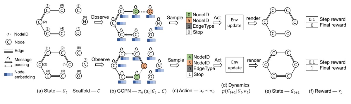
Figure 1: An overview of the proposed iterative graph generation method. Each row corresponds to one step in the generation process. (a) The state is defined as the intermediate graph , and the set of scaffold subgraphs defined as is appended for GCPN calculation. (b) GCPN conducts message passing to encode the state as node embeddings then produce a policy . (c) An action with 4 components is sampled from the policy. (d) The environment performs a chemical valency check on the intermediate state, and then returns (e) the next state and (f) the associated reward .
图 1:所提出的迭代图生成方法概览。每一行对应生成过程中的一步。(a) 状态定义为中间图 ,并把脚手架子图集合 附上,供 GCPN 计算。(b) GCPN 通过消息传递把状态编码为节点嵌入,再产生策略 。(c) 从策略中采样一个含 4 个分量的动作 。(d) 环境对中间状态做化合价检查,然后返回 (e) 下一状态 以及 (f) 相应的奖励 。
3.2 Graph Generation as Markov Decision Process
3.2 作为马尔可夫决策过程的图生成
A key task for building our model is to specify a generation procedure. We designed an iterative graph generation process and formulated it as a general decision process , where is the set of states that consists of all possible intermediate and final graphs, is the set of actions that describe the modification made to current graph at each time step, is the transition dynamics that specifies the possible outcomes of carrying out an action, . is a reward function that specifies the reward after reaching state , and is the discount factor. The procedure to generate a graph can then be described by a trajectory , where is the final generated graph. The modification of a graph at each time step can be viewed as a state transition distribution: , where is usually represented as a policy network .
构建该模型的一项关键任务,是给出生成流程。我们设计了一种迭代的图生成过程,并把它表述为一般决策过程 ,其中 是由所有可能的中间图和最终图组成的状态集合, 是描述每一步对当前图所做修改的动作集合, 是转移动态,用来给出执行某一动作后可能的结果 。 是到达状态 后的奖励函数, 是折扣因子。生成一张图的过程于是可以用一条轨迹 来描述,其中 是最终生成的图。每一步对图的修改可以看成状态转移分布:,其中 通常由策略网络 表示。
Recent graph generation models add nodes and edges based on the full trajectory of the graph generation procedure [43, 25] using recurrent units, which tends to “forget” initial steps of generation quickly. In contrast, we design a graph generation procedure that can be formulated as a Markov Decision Process (MDP), which requires the state transition dynamics to satisfy the Markov property: . Under this property, the policy network only needs the intermediate graph state to derive an action (see Section 3.4). The action is used by the environment to update the intermediate graph being generated (see Section 3.3).
近来的图生成模型往往用循环单元,依据图生成过程的完整轨迹 来添加节点和边 [43, 25],这样很容易很快“忘记”生成初期的步骤。相比之下,我们设计的图生成过程可以表述为马尔可夫决策过程(MDP),要求状态转移动态满足马尔可夫性质:。在这一性质下,策略网络只需中间图状态 即可得到动作(见第 3.4 节)。环境再用该动作更新正在生成的中间图(见第 3.3 节)。
3.3 Molecule Generation Environment
3.3 分子生成环境
In this section we discuss the setup of molecule generation environment. On a high level, the environment builds up a molecular graph step by step through a sequence of bond or substructure addition actions given by GCPN. Figure 1 illustrates the 5 main components that come into play in each step, namely state representation, policy network, action, state transition dynamics and reward. Note that this environment can be easily extended to graph generation tasks in other settings.
本节讨论分子生成环境的设定。概括来说,环境根据 GCPN 给出的一系列加键或加入子结构的动作,一步步搭建分子图。图 1 展示了每一步中起作用的 5 个主要部分:状态表示、策略网络、动作、状态转移动态和奖励。需要说明的是,这一环境也可以较容易地扩展到其他设定下的图生成任务。
State Space. We define the state of the environment as the intermediate generated graph at time step , which is fully observable by the RL agent. Figure 1 (a)(e) depicts the partially generated molecule state before and after an action is taken. At the start of generation, we assume contains a single node that represents a carbon atom.
状态空间。 我们把环境状态 定义为时刻 的中间生成图 ,强化学习智能体可以完全观测到它。图 1 (a)(e) 给出了采取动作前后部分生成的分子状态。生成开始时,我们假定 只含一个代表碳原子的节点。
Action Space. In our framework, we define a distinct, fixed-dimension and homogeneous action space amenable to reinforcement learning. We design an action analogous to link prediction, which is a well studied realm in network science. We first define a set of scaffold subgraphs to be added during graph generation and the collection is defined as . Given a graph at step , we define the corresponding extended graph as . Under this definition, an action can either correspond to connecting a new subgraph to a node in or connecting existing nodes within graph . Once an action is taken, the remaining disconnected scaffold subgraphs are removed. In our implementation, we adopt the most fine-grained version where consists of all different single node graphs, where denotes the number of different atom types. Note that can be extended to contain molecule substructure scaffolds [16], which allows specification of preferred substructures at the cost of model flexibility. In Figure 1(b), a link is predicted between the green and yellow atoms. We will discuss in detail the link prediction algorithm in Section 3.4.
动作空间。 在我们的框架中,我们定义一个明确、维度固定且同质的动作空间,以便于强化学习使用。我们把动作设计成类似于链接预测,这是网络科学中研究较多的问题。首先定义在图生成过程中可加入的脚手架子图集合 ,并把该集合记为 。对第 步的图 ,相应的扩展图定义为 。在此定义下,一个动作既可以是把新的子图 连接到 中的某个节点,也可以是连接 内部已有的节点。一旦采取动作,其余未连接的脚手架子图就被去掉。实现上,我们采用最细粒度的版本: 由全部 种不同的单节点图组成,其中 表示不同原子类型的数目。需要说明的是, 也可以扩展为包含分子亚结构脚手架 [16],这样可以指定偏好的子结构,但会牺牲模型灵活性。在图 1(b) 中,绿色原子和黄色原子之间预测出一条连接。链接预测算法将在第 3.4 节详细讨论。
State Transition Dynamics. Domain-specific rules are incorporated in the state transition dynamics. The environment carries out actions that obey the given rules. Infeasible actions proposed by the policy network are rejected and the state remains unchanged. For the task of molecule generation, the environment incorporates rules of chemistry. In Figure 1(d), both actions pass the valency check, and the environment updates the (partial) molecule according to the actions. Note that unlike a text-based representation, the graph-based molecular representation enables us to perform this step-wise valency check, as it can be conducted even for incomplete molecular graphs.
状态转移动态。 领域特定的规则被纳入状态转移动态中。环境只执行符合给定规则的动作。策略网络提出的不可行动作会被拒绝,状态保持不变。对分子生成任务,环境纳入了化学规则。在图 1(d) 中,两个动作都通过了化合价检查,环境据此更新(部分)分子。需要注意的是,与基于文本的表示不同,基于图的分子表示使我们能够做这种逐步的化合价检查,因为即便分子图还不完整,也可以进行检查。
Reward design. Both intermediate rewards and final rewards are used to guide the behaviour of the RL agent. We define the final rewards as a sum over domain-specific rewards and adversarial rewards. The domain-specific rewards consist of the (combination of) final property scores, such as octanol-water partition coefficient (logP), druglikeness (QED) [1] and molecular weight (MW). Domain-specific rewards also include penalization of unrealistic molecules according to various criteria, such as excessive steric strain and the presence of functional groups that violate ZINC functional group filters [14]. The intermediate rewards include step-wise validity rewards and adversarial rewards. A small positive reward is assigned if the action does not violate valency rules, otherwise a small negative reward is assigned. As an example, the second row of Figure 1 shows the scenario that a termination action is taken. When the environment updates according to a terminating action, both a step reward and a final reward are given, and the generation process terminates.
奖励设计。 中间奖励和最终奖励都用来引导强化学习智能体的行为。我们把最终奖励定义为领域特定奖励与对抗奖励之和。领域特定奖励包括最终性质分数(或其组合),例如辛醇–水分配系数(logP)、药物类似性(QED)[1] 和分子量(MW)。领域特定奖励也包括按多种标准对不现实分子的惩罚,例如过大的空间张力,以及出现违反 ZINC 官能团过滤器的官能团 [14]。中间奖励包括逐步合法性奖励和对抗奖励。若动作不违反化合价规则,则给予小的正奖励,否则给予小的负奖励。例如,图 1 的第二行展示了采取终止动作的情形。当环境按终止动作更新时,会同时给出一步奖励和最终奖励,生成过程随之结束。
To ensure that the generated molecules resemble a given set of molecules, we employ the Generative Adversarial Network (GAN) framework [10] to define the adversarial rewards
为使生成的分子接近给定的一组分子,我们采用生成对抗网络(GAN)框架 [10] 来定义对抗奖励
where is the policy network, is the discriminator network, represents an input graph, is the underlying data distribution which defined either over final graphs (for final rewards) or intermediate graphs (for intermediate rewards). However, only can be trained with stochastic gradient descent, as is a graph object that is non-differentiable with respect to parameters . Instead, we use as an additional reward together with other rewards, and optimize the total rewards with policy gradient methods [44] (Section 3.5). The discriminator network employs the same structure of the policy network (Section 3.4) to calculate the node embeddings, which are then aggregated into a graph embedding and cast into a scalar prediction.
其中 是策略网络, 是判别器网络, 表示输入图, 是底层数据分布,它既可以定义在最终图上(用于最终奖励),也可以定义在中间图上(用于中间奖励)。不过,只有 可以用随机梯度下降来训练,因为 是图对象,对参数 不可微。于是我们把 作为额外奖励与其他奖励一起使用,并用策略梯度方法优化总奖励 [44](第 3.5 节)。判别器网络采用与策略网络相同的结构(第 3.4 节)来计算节点嵌入,再聚合成图嵌入并映射成一个标量预测。
3.4 Graph Convolutional Policy Network
3.4 图卷积策略网络
Having illustrated the graph generation environment, we outline the architecture of GCPN, a policy network learned by the RL agent to act in the environment. GCPN takes the intermediate graph and the collection of scaffold subgraphs as inputs, and outputs the action , which predicts a new link to be added, as described in Section 3.3.
在说明图生成环境之后,我们概述 GCPN 的结构。它是强化学习智能体在环境中行动所学习的策略网络。GCPN 以中间图 和脚手架子图集合 为输入,输出动作 ,用于预测要添加的新连接,如第 3.3 节所述。
Computing node embeddings. In order to perform link prediction in , our model first computes the node embeddings of an input graph using Graph Convolutional Networks (GCN) [20, 5, 18, 36, 8], a well-studied technique that achieves state-of-the-art performance in representation learning for molecules. We use the following variant that supports the incorporation of categorical edge types. The high-level idea is to perform message passing over each edge type for a total of layers. At the th layer of the GCN, we aggregate all messages from different edge types to compute the next layer node embedding , where are the sizes of and respectively, and is the embedding dimension. More concretely,
计算节点嵌入。 为了在 上做链接预测,模型首先用图卷积网络(GCN)[20, 5, 18, 36, 8] 计算输入图的节点嵌入。这是分子表示学习中研究较多、表现也较好的技术。我们采用下面这种支持纳入类别边类型的变体。其主要想法是:对每种边类型做消息传递,一共进行 层。在 GCN 的第 层,我们聚合来自不同边类型的全部消息,计算下一层节点嵌入 ,其中 、 分别是 和 的规模, 是嵌入维数。更具体地,
where is the th slice of edge-conditioned adjacency tensor , and ; . is a trainable weight matrix for the th edge type, and is the node representation learned in the th layer. We use to denote an aggregation function that could be one of [12]. This variant of the GCN layer allows for parallel implementation while remaining expressive for aggregating information among different edge types. We apply a layer GCN to the extended graph to compute the final node embedding matrix .
其中 是边条件邻接张量 的第 个切片,并且 ;。 是第 种边类型的可训练权重矩阵, 是第 层学到的节点表示。我们用 表示聚合函数,可以是 之一 [12]。这种 GCN 层变体既可以并行实现,又足以在不同边类型之间聚合信息。我们对扩展图 应用 层 GCN,得到最终的节点嵌入矩阵 。
Action prediction. The link prediction based action at time step is a concatenation of four components: selection of two nodes, prediction of edge type, and prediction of termination. Concretely, each component is sampled according to a predicted distribution governed by Equation 3 and 4.
动作预测。 第 步基于链接预测的动作 ,是四个分量的拼接:选择两个节点、预测边类型,以及预测是否终止。具体来说,每个分量都按式 (3) 和 (4) 所给出的预测分布来采样。
$$\begin{aligned}
f_{\mathrm{first}}(s_t) &= \mathrm{SOFTMAX}(m_f(X)), & a_{\mathrm{first}} &\sim f_{\mathrm{first}}(s_t) \in {0,1}^n \
f_{\mathrm{second}}(s_t) &= \mathrm{SOFTMAX}(m_s(X_{a_{\mathrm{first}}}, X)), & a_{\mathrm{second}} &\sim f_{\mathrm{second}}(s_t) \in {0,1}^{n+c} \
f_{\mathrm{edge}}(s_t) &= \mathrm{SOFTMAX}(m_e(X_{a_{\mathrm{first}}}, X_{a_{\mathrm{second}}})), & a_{\mathrm{edge}} &\sim f_{\mathrm{edge}}(s_t) \in {0,1}^b \
f_{\mathrm{stop}}(s_t) &= \mathrm{SOFTMAX}(m_t(\mathrm{AGG}(X))), & a_{\mathrm{stop}} &\sim f_{\mathrm{stop}}(s_t) \in {0,1}
\end{aligned} \tag{4}$$
We use to denote a Multilayer Perceptron (MLP) that maps to a vector, which represents the probability distribution of selecting each node. The information from the first selected node is incorporated in the selection of the second node by concatenating its embedding with that of each node in . The second MLP then maps the concatenated embedding to the probability distribution of each potential node to be selected as the second node. Note that when selecting two nodes to predict a link, the first node to select, , should always belong to the currently generated graph , whereas the second node to select, , can be either from (forming a cycle), or from (adding a new substructure). To predict a link, takes and as inputs and maps to a categorical edge type using an MLP. Finally, the termination probability is computed by firstly aggregating the node embeddings into a graph embedding using an aggregation function , and then mapping the graph embedding to a scalar using an MLP .
我们用 表示一个多层感知机(MLP),它把 映射成 向量,表示选择各个节点的概率分布。第一个被选节点 的信息,通过把它的嵌入 与 中每个节点的嵌入拼接,纳入第二个节点的选择。第二个 MLP 再把拼接后的嵌入映射为各个候选节点被选为第二节点的概率分布。需要注意的是,在选择两个节点来预测一条连接时,首先选出的节点 必须属于当前已生成的图 ,而第二个节点 既可以来自 (形成环),也可以来自 (加入新的子结构)。为预测一条连接, 以 和 为输入,用一个 MLP 映射到类别型边类型。最后,终止概率的计算是:先用聚合函数 把节点嵌入聚合成图嵌入,再用 MLP 把图嵌入映射成一个标量。
3.5 Policy Gradient Training
3.5 策略梯度训练
Policy gradient based methods are widely adopted for optimizing policy networks. Here we adopt Proximal Policy Optimization (PPO) [35], one of the state-of-the-art policy gradient methods. The objective function of PPO is defined as follows
基于策略梯度的方法被广泛用于优化策略网络。这里我们采用近端策略优化(PPO)[35],它是当时最优的策略梯度方法之一。PPO 的目标函数定义如下
where is the probability ratio that is clipped to the range of , making the a lower bound of the conservative policy iteration objective [17], is the estimated advantage function which involves a learned value function to reduce the variance of estimation. In GCPN, is an MLP that maps the graph embedding computed according to Section 3.4.
其中 是被裁剪到区间 的概率比,这使得 成为保守策略迭代目标的下界 [17]; 是估计的优势函数,其中用到一个学到的价值函数 来降低估计方差。在 GCPN 中, 是一个 MLP,它把按第 3.4 节计算出的图嵌入映射为价值。
It is known that pretraining a policy network with expert policies if they are available leads to better training stability and performance [24]. In our setting, any ground truth molecule could be viewed as an expert trajectory for pretraining GCPN. This expert imitation objective can be written as , where pairs are obtained from ground truth molecules. Specifically, given a molecule dataset, we randomly sample a molecular graph , and randomly select one connected subgraph of as the state . At state , any action that adds an atom or bond in can be taken in order to generate the sampled molecule. Hence, we randomly sample , and use the pair to supervise the expert imitation objective.
已知若有专家策略可用,用它们对策略网络做预训练,会带来更好的训练稳定性和表现 [24]。在我们的设定里,任何真值分子都可以看作预训练 GCPN 的专家轨迹。这一专家模仿目标可以写成 ,其中 对来自真值分子。具体来说,给定一个分子数据集,我们随机采样一张分子图 ,再随机选出 的一个连通子图 作为状态 。在状态 下,任何向 中添加原子或键的动作,都可以用来生成这个被采样的分子。因此,我们随机采样 ,并用 对来监督专家模仿目标。
4 Experiments
4 实验
To demonstrate effectiveness of goal-directed search for molecules with desired properties, we compare our method with state-of-the-art molecule generation algorithms in the following tasks.
为说明面向目标地搜索具有期望性质的分子是否有效,我们在下列任务上与当时最优的分子生成算法进行比较。
Property Optimization. The task is to generate novel molecules whose specified molecular properties are optimized. This can be useful in many applications such as drug discovery and materials science, where the goal is to identify molecules with highly optimized properties of interest.
性质优化。 任务是生成指定分子性质得到优化的新分子。这在药物发现和材料科学等许多应用中都很有用,目标是找出所关心性质被高度优化的分子。
Property Targeting. The task is to generate novel molecules whose specified molecular properties are as close to the target scores as possible. This is crucial in generating virtual libraries of molecules with properties that are generally suitable for a desired application. For example, a virtual molecule library for drug discovery should have high drug-likeness and synthesizability.
性质定向。 任务是生成指定分子性质尽可能接近目标分数的新分子。这在构建性质大体适合某一应用的虚拟分子库时至关重要。例如,用于药物发现的虚拟分子库应当具有较高的药物类似性和可合成性。
Constrained Property Optimization. The task is to generate novel molecules whose specified molecular properties are optimized, while also containing a specified molecular substructure. This can be useful in lead optimization problems in drug discovery and materials science, where we want to make modifications to a promising lead molecule and improve its properties [2].
带约束的性质优化。 任务是生成指定分子性质得到优化、同时又含有指定分子亚结构的新分子。这在药物发现和材料科学中的先导优化问题上很有用:我们希望对一个有前景的先导分子做修改,并改进其性质 [2]。
4.1 Experimental Setup
4.1 实验设置
We outline our experimental setup in this section. Further details are provided in the appendix¹.
本节概述实验设置。更多细节见附录¹。
¹Link to code and datasets: https://github.com/bowenliu16/rl_graph_generation
Dataset. For the molecule generation experiments, we utilize the ZINC250k molecule dataset [14] that contains 250,000 drug like commercially available molecules whose maximum atom number is 38. We use the dataset for both expert pretraining and adversarial training.
数据集。 在分子生成实验中,我们使用 ZINC250k 分子数据集 [14],其中包含 250,000 个可商购的类药分子,最大原子数为 38。该数据集同时用于专家预训练和对抗训练。
Molecule environment. We set up the molecule environment as an OpenAI Gym environment [3] using RDKit [23] and adapt it to the ZINC250k dataset. Specifically, the maximum atom number is set to be 38. There are 9 atom types and 3 edge types, as molecules are represented in kekulized form. For specific reward design, we linearly scale each reward component according to its importance in molecule generation from a chemistry point of view as well as the quality of generation results. When summing up all the rewards collected from a molecule generation trajectory, the range of the reward value that the model can get is for final chemical property reward, for final chemical filter reward, for final adversarial reward, for intermediate adversarial reward and for intermediate validity reward.
分子环境。 我们用 RDKit [23] 把分子环境做成一个 OpenAI Gym 环境 [3],并使其适配 ZINC250k 数据集。具体来说,最大原子数设为 38。由于分子以 kekulé 形式表示,共有 9 种原子类型和 3 种边类型。在具体奖励设计上,我们根据各奖励分量在化学意义上对分子生成的重要性,以及生成结果的质量,对它们做线性缩放。把一条分子生成轨迹上收集到的全部奖励加总后,模型可获得的奖励取值范围是:最终化学性质奖励 ,最终化学过滤奖励 ,最终对抗奖励 ,中间对抗奖励 ,中间合法性奖励 。
Table 1: Comparison of the top 3 property scores of generated molecules found by each model.
| Method | Penalized logP | QED | ||||||
|---|---|---|---|---|---|---|---|---|
| 1st | 2nd | 3rd | Validity | 1st | 2nd | 3rd | Validity | |
| ZINC | 4.52 | 4.30 | 4.23 | 100.0% | 0.948 | 0.948 | 0.948 | 100.0% |
| Hill Climbing | − | − | − | − | 0.838 | 0.814 | 0.814 | 100.0% |
| ORGAN | 3.63 | 3.49 | 3.44 | 0.4% | 0.896 | 0.824 | 0.820 | 2.2% |
| JT-VAE | 5.30 | 4.93 | 4.49 | 100.0% | 0.925 | 0.911 | 0.910 | 100.0% |
| GCPN | 7.98 | 7.85 | 7.80 | 100.0% | 0.948 | 0.947 | 0.946 | 100.0% |
表 1:各模型找到的生成分子中前 3 个性质分数的比较。
| Method | Penalized logP | QED | ||||||
|---|---|---|---|---|---|---|---|---|
| 1st | 2nd | 3rd | Validity | 1st | 2nd | 3rd | Validity | |
| ZINC | 4.52 | 4.30 | 4.23 | 100.0% | 0.948 | 0.948 | 0.948 | 100.0% |
| Hill Climbing | − | − | − | − | 0.838 | 0.814 | 0.814 | 100.0% |
| ORGAN | 3.63 | 3.49 | 3.44 | 0.4% | 0.896 | 0.824 | 0.820 | 2.2% |
| JT-VAE | 5.30 | 4.93 | 4.49 | 100.0% | 0.925 | 0.911 | 0.910 | 100.0% |
| GCPN | 7.98 | 7.85 | 7.80 | 100.0% | 0.948 | 0.947 | 0.946 | 100.0% |
GCPN Setup. We use a 3-layer defined GCPN as the policy network with 64 dimensional node embedding in all hidden layers, and batch normalization [13] is applied after each layer. Another 3-layer GCN with the same architecture is used for discriminator training. We find little improvement when further adding GCN layers. We observe comparable performance among different aggregation functions and select for all experiments. We found both the expert pretraining and RL objective important for generating high quality molecules, thus both of them are kept throughout training. Specifically, we use PPO algorithm to train the RL objective with the default hyperparameters as we do not observe too much performance gain from tuning these hyperparameters, and the learning rate is set as 0.001. The expert pretraining objective is trained with a learning rate of 0.00025, and we do observe that adding this objective contributes to faster convergence and better performance. Both objectives are trained using Adam optimizer [19] with batch size 32.
GCPN 设置。 我们使用一个定义为 3 层的 GCPN 作为策略网络,所有隐层的节点嵌入都是 64 维,并且在每一层之后施加批归一化 [13]。判别器训练使用另一个结构相同的 3 层 GCN。我们发现再增加 GCN 层几乎没有改进。不同聚合函数的表现相近,全部实验都选用 。我们发现专家预训练和强化学习目标对生成高质量分子都很重要,因此在整个训练过程中同时保留二者。具体来说,我们用 PPO 算法、默认超参数来训练强化学习目标,因为调节这些超参数并没有带来太多收益,学习率设为 0.001。专家预训练目标的学习率设为 0.00025,我们也确实观察到加入这一目标有助于更快收敛、表现更好。两个目标都用 Adam 优化器 [19] 训练,批量大小为 32。
Baselines. We compare our method with the following state-of-the-art baselines. Junction Tree VAE (JT-VAE) [16] is a state-of-the-art algorithm that combines graph representation and a VAE framework for generating molecular graphs, and uses Bayesian optimization over the learned latent space to search for molecules with optimized property scores. JT-VAE has been shown to outperform previous deep generative models for molecule generation, including Character-VAE [9], Grammar-VAE [22], SD-VAE [4] and GraphVAE [39]. We also compare our approach with ORGAN [27], a state-of-the-art RL-based molecule generation algorithm using a text-based representation of molecules. To demonstrate the benefits of learning-based approaches, we further implement a simple rule based model using the stochastic hill-climbing algorithm. We start with a graph containing a single atom (the same setting as GCPN), traverse all valid actions given the current state, randomly pick the next state with top 5 highest property score as long as there is improvement over the current state, and loop until reaching the maximum number of nodes. To make fair comparison across different methods, we set up the same objective functions for all methods, and run all the experiments on the same computing facilities using 32 CPU cores. We run both deep learning baselines using their released code and allow the baselines to have wall clock running time for roughly 24 hours, while our model can get the results in roughly 8 hours.
基线。 我们与下列当时最优的基线进行比较。连接树变分自编码器(JT-VAE)[16] 是一种把图表示与 VAE 框架结合起来生成分子图的先进算法,并在学到的潜空间上用贝叶斯优化搜索性质分数被优化的分子。已有结果表明,JT-VAE 超过了此前的深度分子生成模型,包括 Character-VAE [9]、Grammar-VAE [22]、SD-VAE [4] 和 GraphVAE [39]。我们还与 ORGAN [27] 比较,这是一种当时最优的、基于强化学习、并采用文本分子表示的生成算法。为说明基于学习的方法的好处,我们还实现了一个简单的基于规则的模型,采用随机爬山算法:从图中只含一个原子开始(与 GCPN 相同的设定),遍历当前状态下所有合法动作,只要相对当前状态有改进,就从性质分数最高的前 5 个下一状态中随机选取,循环直到达到最大节点数。为公平比较不同方法,我们对所有方法设置相同的目标函数,并在同一计算设施上用 32 个 CPU 核心运行全部实验。两个深度学习基线都使用其发布的代码,并允许它们大约运行 24 小时的墙上时间,而我们的模型大约 8 小时即可得到结果。
4.2 Molecule Generation Results
4.2 分子生成结果
Property optimization. In this task, we focus on generating molecules with the highest possible penalized logP [22] and QED [1] scores. Penalized logP is a logP score that also accounts for ring size and synthetic accessibility [6], while QED is an indicator of drug-likeness. Note that both scores are calculated from empirical prediction models whose parameters are estimated from related datasets [41, 1], and these scores are widely used in previous molecule generation papers [9, 22, 4, 39, 27]. Penalized logP has an unbounded range, while the QED has a range of by definition, thus directly comparing the percentage improvement of QED may not be meaningful. We adopt the same evaluation method in previous approaches [22, 4, 16], reporting the best 3 property scores found by each model and the fraction of molecules that satisfy chemical validity. Table 1 summarizes the best property scores of molecules found by each model, and the statistics in ZINC250k is also shown for comparison. Our method consistently performs significantly better than previous methods when optimizing penalized logP, achieving an average improvement of 61% compared to JT-VAE, and 186% compared to ORGAN. Our method outperforms all the baselines in the QED optimization task as well, and significantly outperforms the stochastic hill climbing baseline.
性质优化。 在这一任务中,我们关注生成惩罚 logP [22] 和 QED [1] 分数尽可能高的分子。惩罚 logP 是在 logP 之外还考虑环大小和合成可及性 [6] 的分数,QED 则是药物类似性的指标。需要说明的是,这两个分数都由经验预测模型计算,其参数从相关数据集估计得到 [41, 1],并在以往的分子生成论文中被广泛使用 [9, 22, 4, 39, 27]。惩罚 logP 的取值范围没有上界,而 QED 按定义在 内,因此直接比较 QED 的百分比提升可能没有意义。我们采用与已有方法 [22, 4, 16] 相同的评价方式,报告每个模型找到的最好 3 个性质分数,以及满足化学合法性的分子比例。表 1 汇总了各模型找到的分子的最好性质分数,并给出 ZINC250k 中的统计量供对照。在优化惩罚 logP 时,我们的方法持续明显优于已有方法,相对 JT-VAE 平均提高 61%,相对 ORGAN 提高 186%。在 QED 优化任务上,我们的方法也超过全部基线,并显著优于随机爬山基线。
Compared with ORGAN, our model can achieve a perfect validity ratio due to the molecular graph representation that allows for step-wise chemical valency check. Compared to JT-VAE, our model can reach a much higher score owing to the fact that RL allows for direct optimization of a given property score and is able to easily extrapolate beyond the given dataset. Visualizations of generated molecules with optimized logP and QED scores are displayed in Figure 2(a) and (b) respectively.
与 ORGAN 相比,由于分子图表示允许逐步做化合价检查,我们的模型可以达到完全合法。与 JT-VAE 相比,我们的模型能达到高得多的分数,因为强化学习可以直接优化给定的性质分数,并且容易外推到给定数据集之外。优化 logP 和 QED 分数后生成的分子,分别在图 2(a) 和 (b) 中可视化。
Although most generated molecules are realistic, in some very rare cases, especially where we reduce the of the adversarial reward and expert pretraining components, our method can generate undesirable molecules with astonishingly high penalized logP predicted by the empirical model, such as the one on the bottom-right of Figure 2(a) in which our method correctly identified that Iodine has the highest per atom contribution in the empirical model used to calculate logP. These undesirable molecules are likely to have inaccurate predicted properties and illustrate an issue with optimizing properties calculated by an empirical model, such as penalized logP and QED, without incorporating prior knowledge. Empirical prediction models that predict molecular properties generalize poorly for molecules that are significantly different from the set of molecules used to train the model. Without any restrictions on the generated molecules, an optimization algorithm would exploit the lack of generalizability of the empirical property prediction models in certain areas of molecule space. Our model addresses this issue by incorporating prior knowledge of known realistic molecules using adversarial training and expert pretraining, which results in more realistic molecules, but with lower property scores calculated by the empirical prediction models. Note that the hill climbing baseline algorithm mostly generates undesirable cases where the accuracy of the empirical prediction model is questionable, thus its performance with optimizing penalized logP is not listed on Table 1.
尽管大多数生成的分子是真实的,但在极少数情况下,尤其是当我们减弱对抗奖励和专家预训练分量时,该方法可能生成经验模型预测出高得惊人的惩罚 logP、却并不理想的分子。例如图 2(a) 右下角的那个分子:我们的方法正确地识别出,在用来计算 logP 的经验模型中,碘的逐原子贡献最高。这些不理想的分子很可能性质预测并不准确,也说明了在不纳入先验知识的情况下,去优化由经验模型算出的性质(如惩罚 logP 和 QED)会有什么问题。预测分子性质的经验模型,对与训练所用分子差别很大的分子泛化较差。若对生成分子不加限制,优化算法就会利用经验性质预测模型在分子空间某些区域缺乏泛化这一点。我们的模型通过对抗训练和专家预训练纳入已知真实分子的先验知识,从而得到更真实的分子,只是由经验预测模型算出的性质分数会低一些。需要说明的是,爬山基线算法大多会生成经验预测模型准确性存疑的不理想情形,因此它在优化惩罚 logP 上的表现未列入表 1。
Property Targeting. In this task, we specify a target range for molecular weight (MW) and logP, and report the percentage of generated molecules with property scores within the range, as well as the diversity of generated molecules. The diversity of a set of molecules is defined as the average pairwise Tanimoto distance between the Morgan fingerprints [33] of the molecules. The RL reward for this task is the L1 distance between the property score of a generated molecule and the range center. To increase the difficulty, we set the target range such that few molecules in ZINC250k dataset are within the range to test the extrapolation ability of the methods to optimize for a given target. The target ranges include , , and .
性质定向。 在这一任务中,我们为分子量(MW)和 logP 指定目标区间,报告生成分子中性质分数落在该区间内的比例,以及生成分子的多样性。一组分子的多样性定义为这些分子的 Morgan 指纹 [33] 之间两两 Tanimoto 距离的平均值。该任务的强化学习奖励,是生成分子的性质分数与区间中心之间的 L1 距离。为增加难度,我们把目标区间设成 ZINC250k 数据集中只有很少分子落在其中,以检验各方法为给定目标做优化时的外推能力。目标区间包括 、、 以及 。
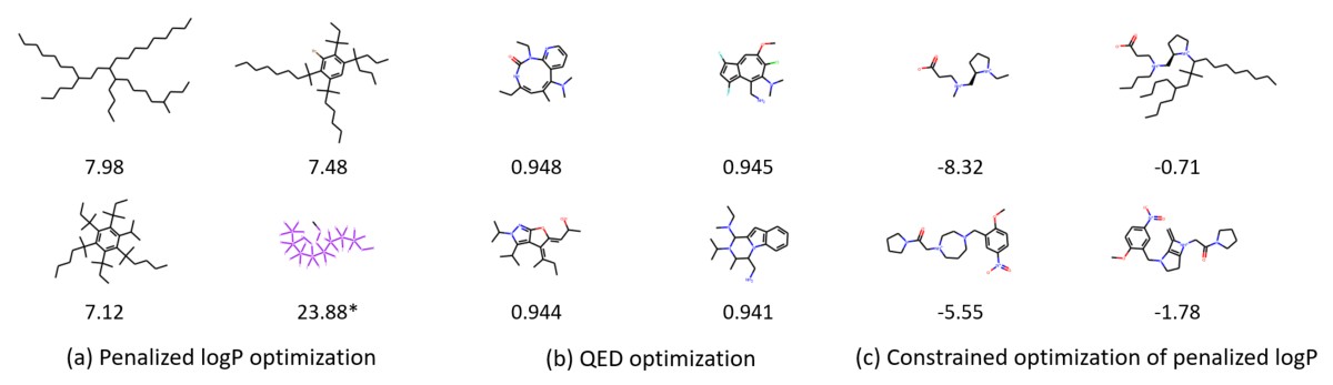
Figure 2: Samples of generated molecules in property optimization and constrained property optimization task. In (c), the two columns correspond to molecules before and after modification.
图 2:性质优化和带约束性质优化任务中生成的分子样本。在 (c) 中,两列分别对应修改前和修改后的分子。
Table 2: Comparison of the effectiveness of property targeting task.
| Method | ||||||||
|---|---|---|---|---|---|---|---|---|
| Success | Diversity | Success | Diversity | Success | Diversity | Success | Diversity | |
| ZINC | 0.3% | 0.919 | 1.3% | 0.909 | 1.7% | 0.938 | 0 | − |
| JT-VAE | 11.3% | 0.846 | 7.6% | 0.907 | 0.7% | 0.824 | 16.0% | 0.898 |
| ORGAN | 0 | − | 0.2% | 0.909 | 15.1% | 0.759 | 0.1% | 0.907 |
| GCPN | 85.5% | 0.392 | 54.7% | 0.855 | 76.1% | 0.921 | 74.1% | 0.920 |
表 2:性质定向任务有效性的比较。
| Method | ||||||||
|---|---|---|---|---|---|---|---|---|
| Success | Diversity | Success | Diversity | Success | Diversity | Success | Diversity | |
| ZINC | 0.3% | 0.919 | 1.3% | 0.909 | 1.7% | 0.938 | 0 | − |
| JT-VAE | 11.3% | 0.846 | 7.6% | 0.907 | 0.7% | 0.824 | 16.0% | 0.898 |
| ORGAN | 0 | − | 0.2% | 0.909 | 15.1% | 0.759 | 0.1% | 0.907 |
| GCPN | 85.5% | 0.392 | 54.7% | 0.855 | 76.1% | 0.921 | 74.1% | 0.920 |
As is shown in Table 2, GCPN has a significantly higher success rate in generating molecules with properties within the target range, compared to baseline methods. In addition, GCPN is able to generate molecules with high diversity, indicating that it is capable of learning a general stochastic policy to generate molecular graphs that fulfill the property requirements.
如表 2 所示,与基线方法相比,GCPN 在生成性质落在目标区间内的分子上成功率明显更高。此外,GCPN 还能生成多样性较高的分子,表明它能够学到一个通用的随机策略,用于生成满足性质要求的分子图。
Constrained Property Optimization. In this experiment, we optimize the penalized logP while constraining the generated molecules to contain one of the 800 ZINC molecules with low penalized logP, following the evaluation in JT-VAE. Since JT-VAE cannot constrain the generated molecule to have certain structure, we adopt their evaluation method where the constraint is relaxed such that the molecule similarity between the original and modified molecules is above a threshold .
带约束的性质优化。 在本实验中,我们优化惩罚 logP,同时约束生成的分子包含 800 个低惩罚 logP 的 ZINC 分子之一,评价方式沿用 JT-VAE。由于 JT-VAE 不能约束生成分子具有特定结构,我们采用他们的评价方法:把约束放宽为原始分子与修改后分子之间的相似度 高于阈值 。
Table 3: Comparison of the performance in the constrained optimization task.
| JT-VAE | GCPN | |||||
|---|---|---|---|---|---|---|
| Improvement | Similarity | Success | Improvement | Similarity | Success | |
| 0.0 | 97.5% | 100.0% | ||||
| 0.2 | 97.1% | 100.0% | ||||
| 0.4 | 83.6% | 100.0% | ||||
| 0.6 | 46.4% | 100.0% |
表 3:带约束优化任务中的表现比较。
| JT-VAE | GCPN | |||||
|---|---|---|---|---|---|---|
| Improvement | Similarity | Success | Improvement | Similarity | Success | |
| 0.0 | 97.5% | 100.0% | ||||
| 0.2 | 97.1% | 100.0% | ||||
| 0.4 | 83.6% | 100.0% | ||||
| 0.6 | 46.4% | 100.0% |
We train a fixed GCPN in an environment whose initial state is randomly set to be one of the 800 ZINC molecules, then conduct the same training procedure as the property optimization task. Over the 800 molecules, the mean and standard deviation of the highest property score improvement and the corresponding similarity between the original and modified molecules are reported in Table 3. Our model significantly outperforms JT-VAE with 184% higher penalized logP improvement on average, and consistently succeeds in discovering molecules with higher logP scores. Also note that JT-VAE performs optimization steps for each given molecule constraint. In contrast, GCPN can generalize well: it learns a general policy to improve property scores, and applies the same policy to all 800 molecules. Figure 2(c) shows that GCPN can modify ZINC molecules to achieve high penalized logP score while still containing the substructure of the original molecule.
我们在一个初始状态被随机设为这 800 个 ZINC 分子之一的环境中训练固定的 GCPN,训练流程与性质优化任务相同。在这 800 个分子上,最高性质分数提升的均值和标准差,以及原始分子与修改后分子之间的相应相似度,报告在表 3 中。我们的模型显著超过 JT-VAE,惩罚 logP 的平均提升高出 184%,并且始终能够发现 logP 分数更高的分子。还需要注意的是,JT-VAE 要对每一个给定的分子约束分别做优化步骤。相比之下,GCPN 的泛化更好:它学到一个改进性质分数的通用策略,并把同一策略应用到全部 800 个分子上。图 2(c) 表明,GCPN 可以修改 ZINC 分子以获得较高的惩罚 logP 分数,同时仍保留原分子的亚结构。
5 Conclusion
5 结论
We introduced GCPN, a graph generation policy network using graph state representation and adversarial training, and applied it to the task of goal-directed molecular graph generation. GCPN consistently outperforms other state-of-the-art approaches in the tasks of molecular property optimization and targeting, and at the same time, maintains 100% validity and resemblance to realistic molecules. Furthermore, the application of GCPN can extend well beyond molecule generation. The algorithm can be applied to generate graphs in many contexts, such as electric circuits, social networks, and explore graphs that can optimize certain domain specific properties.
我们提出了 GCPN,这是一种使用图状态表示和对抗训练的图生成策略网络,并把它用于面向目标的分子图生成。GCPN 在分子性质优化和定向任务上持续超过其他当时最优的方法,同时又保持 100% 合法,并接近真实分子。此外,GCPN 的应用可以远远超出分子生成。该算法可用于在许多情境下生成图,例如电路、社交网络,并探索能够优化某些领域特定性质的图。
6 Acknowledgements
6 致谢
The authors thank Xiang Ren, Marinka Zitnik, Jiaming Song, Joseph Gomes, Amir Barati Farimani, Peter Eastman, Franklin Lee, Zhenqin Wu and Paul Wender for their helpful discussions. This research has been supported in part by DARPA SIMPLEX, ARO MURI, Stanford Data Science Initiative, Huawei, JD, and Chan Zuckerberg Biohub. The Pande Group acknowledges the generous support of Dr. Anders G. Frøseth and Mr. Christian Sundt for our work on machine learning. The Pande Group is broadly supported by grants from the NIH (R01 GM062868 and U19 AI109662) as well as gift funds and contributions from Folding@home donors.
作者感谢 Xiang Ren、Marinka Zitnik、Jiaming Song、Joseph Gomes、Amir Barati Farimani、Peter Eastman、Franklin Lee、Zhenqin Wu 和 Paul Wender 的有益讨论。本研究部分得到 DARPA SIMPLEX、ARO MURI、Stanford Data Science Initiative、Huawei、JD 以及 Chan Zuckerberg Biohub 的支持。Pande 研究组感谢 Anders G. Frøseth 博士和 Christian Sundt 先生对我们机器学习工作的慷慨支持。Pande 研究组还广泛得到 NIH 资助(R01 GM062868 和 U19 AI109662)以及 Folding@home 捐助者的赠款和捐助。
V.S.P. is a consultant & SAB member of Schrodinger, LLC and Globavir, sits on the Board of Directors of Apeel Inc, Asimov Inc, BioAge Labs, Freenome Inc, Omada Health, Patient Ping, Rigetti Computing, and is a General Partner at Andreessen Horowitz.
V.S.P. 是 Schrodinger, LLC 和 Globavir 的顾问及科学顾问委员会成员,担任 Apeel Inc、Asimov Inc、BioAge Labs、Freenome Inc、Omada Health、Patient Ping、Rigetti Computing 的董事会成员,并担任 Andreessen Horowitz 的普通合伙人。
7 Appendix
7 附录
Validity. We define a molecule as valid if it is able to pass the sanitization checks in RDKit.
合法性。 若一个分子能够通过 RDKit 中的清洗检查,我们就把它定义为合法。
Valency. This specifies the chemically allowable node degrees for an atom of a particular element. Some elements can have multiple possible valencies. At each intermediate step, the molecule environment checks that each atom in the partially completed graph has not exceeded its maximum possible valency of that element type.
化合价。 它规定某一元素的原子在化学上允许的节点度数。有些元素可以有多种可能的化合价。在每一个中间步骤,分子环境都会检查部分完成的图中每个原子是否尚未超过该元素类型的最大可能化合价。
Steric strain filter. Valid molecules can still be unrealistic. In particular, it is possible to generate valid molecules that are very sterically strained such that it is unlikely that they will be stable at ordinary conditions. We designed a simple steric strain filter that performs MMFF94 forcefield [11] minimization on a molecule, and then penalizes it as being too sterically strained if the average angle bend energy exceeds a cutoff of 0.82 kcal/mol.
空间张力过滤器。 合法的分子仍可能并不现实。特别是,有可能生成在空间上非常紧张、因而不太可能在普通条件下稳定的合法分子。我们设计了一个简单的空间张力过滤器:先对分子做 MMFF94 力场 [11] 最小化,若平均键角弯曲能量超过 0.82 kcal/mol 的阈值,就将其作为空间张力过大予以惩罚。
Reactive functional group filter. We also penalize molecules that possess known problematic and reactive functional groups. For simplicity, we use the same set of rules that was used in the construction of the ZINC dataset, as implemented in RDKit.
反应性官能团过滤器。 我们也会惩罚含有已知有问题、易反应官能团的分子。为简便起见,我们使用构建 ZINC 数据集时所用的同一套规则,实现来自 RDKit。
Reward design implementation. For property optimization task, we use linear functions to roughly map the minimum and maximum property score of ZINC dataset into the desired reward range. For property targeting task, we use linear functions to map the absolute difference between the target and the property score into the desired reward range. We threshold the reward such that the reward will not exceed the desired reward range, as is described in Section 4.1. For specific parameters, please refer to the open-sourced code: https://github.com/bowenliu16/rl_graph_generation
奖励设计的实现。 对性质优化任务,我们用线性函数把 ZINC 数据集中性质分数的最小和最大值大致映射到期望的奖励范围。对性质定向任务,我们用线性函数把目标与性质分数之差的绝对值映射到期望的奖励范围。我们再对奖励设阈值,使其不超过期望范围,如第 4.1 节所述。具体参数请参见开源代码:https://github.com/bowenliu16/rl_graph_generation
References
参考文献
[1] G. R. Bickerton, G. V. Paolini, J. Besnard, S. Muresan, and A. L. Hopkins. Quantifying the chemical beauty of drugs. Nature chemistry, 4(2):90, 2012.
[2] K. H. Bleicher, H.-J. Böhm, K. Müller, and A. I. Alanine. Hit and lead generation: beyond high-throughput screening. Nature Reviews Drug Discovery, 2:369–378, 2003.
[3] G. Brockman, V. Cheung, L. Pettersson, J. Schneider, J. Schulman, J. Tang, and W. Zaremba. Openai gym. CoRR, abs/1606.01540, 2016.
[4] H. Dai, Y. Tian, B. Dai, S. Skiena, and L. Song. Syntax-directed variational autoencoder for structured data. arXiv preprint arXiv:1802.08786, 2018.
[5] D. K. Duvenaud, D. Maclaurin, J. Iparraguirre, R. Bombarell, T. Hirzel, A. Aspuru-Guzik, and R. P. Adams. Convolutional networks on graphs for learning molecular fingerprints. In Advances in neural information processing systems, 2015.
[6] P. Ertl. Estimation of synthetic accessibility score of drug-like molecules. J. Cheminform, 2009.
[7] P. Ertl, R. Lewis, E. J. Martin, and V. Polyakov. In silico generation of novel, drug-like chemical matter using the LSTM neural network. CoRR, abs/1712.07449, 2017.
[8] J. Gilmer, S. S. Schoenholz, P. F. Riley, O. Vinyals, and G. E. Dahl. Neural message passing for quantum chemistry, 2017.
[9] R. Gómez-Bombarelli, J. N. Wei, D. Duvenaud, J. M. Hernández-Lobato, B. Sánchez-Lengeling, D. Sheberla, J. Aguilera-Iparraguirre, T. D. Hirzel, R. P. Adams, and A. Aspuru-Guzik. Automatic chemical design using a data-driven continuous representation of molecules. ACS Central Science, 2016.
[10] I. Goodfellow, J. Pouget-Abadie, M. Mirza, B. Xu, D. Warde-Farley, S. Ozair, A. Courville, and Y. Bengio. Generative adversarial nets. In Advances in neural information processing systems, 2014.
[11] T. A. Halgren. Merck molecular force field. i. basis, form, scope, parameterization, and performance of mmff94. Journal of computational chemistry, 17(5-6):490–519, 1996.
[12] W. Hamilton, Z. Ying, and J. Leskovec. Inductive representation learning on large graphs. In Advances in Neural Information Processing Systems, 2017.
[13] S. Ioffe and C. Szegedy. Batch normalization: Accelerating deep network training by reducing internal covariate shift. In F. Bach and D. Blei, editors, Proceedings of the 32nd International Conference on Machine Learning, volume 37 of Proceedings of Machine Learning Research, pages 448–456, Lille, France, 07–09 Jul 2015. PMLR.
[14] J. J. Irwin, T. Sterling, M. M. Mysinger, E. S. Bolstad, and R. G. Coleman. Zinc: a free tool to discover chemistry for biology. Journal of chemical information and modeling, 52(7):1757– 1768, 2012.
[15] E. Jannik Bjerrum and R. Threlfall. Molecular Generation with Recurrent Neural Networks (RNNs). arXiv preprint arXiv:1705.04612, 2017.
[16] W. Jin, R. Barzilay, and T. Jaakkola. Junction tree variational autoencoder for molecular graph generation. arXiv preprint arXiv:1802.04364, 2018.
[17] S. Kakade and J. Langford. Approximately optimal approximate reinforcement learning. In International Conference on Machine Learning, 2002.
[18] S. Kearnes, K. McCloskey, M. Berndl, V. Pande, and P. Riley. Molecular graph convolutions: moving beyond fingerprints. Journal of Computer-Aided Molecular Design, 30:595–608, Aug. 2016.
[19] D. P. Kingma and J. Ba. Adam: A method for stochastic optimization. International Conference on Learning Representations, 2015.
[20] T. N. Kipf and M. Welling. Semi-supervised classification with graph convolutional networks. In ICLR, 2016.
[21] P. Kirkpatrick and C. Ellis. Chemical space. Nature, 432:823 EP –, Dec 2004.
[22] M. J. Kusner, B. Paige, and J. M. Hernández-Lobato. Grammar variational autoencoder. In D. Precup and Y. W. Teh, editors, International Conference on Machine Learning, volume 70 of Proceedings of Machine Learning Research, International Convention Centre, Sydney, Australia, 06–11 Aug 2017. PMLR.
[23] G. Landrum. Rdkit: Open-source cheminformatics. 2006. Google Scholar, 2006.
[24] S. Levine and V. Koltun. Guided policy search. In International Conference on Machine Learning, 2013.
[25] Y. Li, O. Vinyals, C. Dyer, R. Pascanu, and P. Battaglia. Learning deep generative models of graphs. arXiv preprint arXiv:1803.03324, 2018.
[26] Y. Li, L. Zhang, and Z. Liu. Multi-Objective De Novo Drug Design with Conditional Graph Generative Model. ArXiv e-prints, Jan. 2018.
[27] G. Lima Guimaraes, B. Sanchez-Lengeling, C. Outeiral, P. L. Cunha Farias, and A. Aspuru-Guzik. Objective-Reinforced Generative Adversarial Networks (ORGAN) for Sequence Generation Models. ArXiv e-prints, May 2017.
[28] J. H. Lin and A. Y. H. Lu. Role of pharmacokinetics and metabolism in drug discovery and development. Pharmacological Reviews, 49(4):403–449, 1997.
[29] C. A. Lipinski, F. Lombardo, B. W. Dominy, and P. J. Feeney. Experimental and computational approaches to estimate solubility and permeability in drug discovery and development settings. Advanced Drug Delivery Reviews, 23(1):3–25, 1997.
[30] B. Liu, B. Ramsundar, P. Kawthekar, J. Shi, J. Gomes, Q. Luu Nguyen, S. Ho, J. Sloane, P. Wender, and V. Pande. Retrosynthetic reaction prediction using neural sequence-to-sequence models. ACS Central Science, 3(10):1103–1113, 2017.
[31] M. Olivecrona, T. Blaschke, O. Engkvist, and H. Chen. Molecular de-novo design through deep reinforcement learning. Journal of Cheminformatics, 9(1):48, Sep 2017.
[32] P. G. Polishchuk, T. I. Madzhidov, and A. Varnek. Estimation of the size of drug-like chemical space based on gdb-17 data. Journal of Computer-Aided Molecular Design, 27(8):675–679, Aug 2013.
[33] D. Rogers and M. Hahn. Extended-connectivity fingerprints. Journal of chemical information and modeling, 50(5):742–754, 2010.
[34] B. Sanchez-Lengeling, C. Outeiral, G. L. Guimaraes, and A. Aspuru-Guzik. Optimizing distributions over molecular space. An Objective-Reinforced Generative Adversarial Network for Inverse-design Chemistry (ORGANIC). ChemRxiv e-prints, 8 2017.
[35] J. Schulman, F. Wolski, P. Dhariwal, A. Radford, and O. Klimov. Proximal policy optimization algorithms. CoRR, abs/1707.06347, 2017.
[36] K. T. Schütt, F. Arbabzadah, S. Chmiela, K. R. Müller, and A. Tkatchenko. Quantum-chemical insights from deep tensor neural networks. Nature Communications, 8:13890, Jan 2017. Article.
[37] M. D. Segall. Multi-parameter optimization: Identifying high quality compounds with a balance of properties. Current Pharmaceutical Design, 18(9):1292–1310, 2012.
[38] M. H. S. Segler, T. Kogej, C. Tyrchan, and M. P. Waller. Generating focused molecule libraries for drug discovery with recurrent neural networks. ACS Central Science, 4(1):120–131, 2018.
[39] M. Simonovsky and N. Komodakis. Graphvae: Towards generation of small graphs using variational autoencoders. arXiv preprint arXiv:1802.03480, 2018.
[40] D. Weininger. Smiles, a chemical language and information system. 1. introduction to methodology and encoding rules. Journal of chemical information and computer sciences, 28(1):31–36, 1988.
[41] S. A. Wildman and G. M. Crippen. Prediction of physicochemical parameters by atomic contributions. Journal of Chemical Information and Computer Sciences, 39(5):868–873, 1999.
[42] X. Yang, J. Zhang, K. Yoshizoe, K. Terayama, and K. Tsuda. ChemTS: An Efficient Python Library for de novo Molecular Generation. ArXiv e-prints, Sept. 2017.
[43] J. You, R. Ying, X. Ren, W. L. Hamilton, and J. Leskovec. Graphrnn: A deep generative model for graphs. arXiv preprint arXiv:1802.08773, 2018.
[44] L. Yu, W. Zhang, J. Wang, and Y. Yu. Seqgan: Sequence generative adversarial nets with policy gradient. In AAAI, 2017.