Generative Adversarial Imitation Learning

Jonathan Ho Affiliation:  Stanford University Email:  hoj@cs.stanford.edu    Stefano Ermon Affiliation:  Stanford University Email:  ermon@cs.stanford.edu

Abstract

摘要

Consider learning a policy from example expert behavior, without interaction with the expert or access to reinforcement signal. One approach is to recover the expert’s cost function with inverse reinforcement learning, then extract a policy from that cost function with reinforcement learning. This approach is indirect and can be slow. We propose a new general framework for directly extracting a policy from data, as if it were obtained by reinforcement learning following inverse reinforcement learning. We show that a certain instantiation of our framework draws an analogy between imitation learning and generative adversarial networks, from which we derive a model-free imitation learning algorithm that obtains significant performance gains over existing model-free methods in imitating complex behaviors in large, high-dimensional environments.

考虑从示例专家行为中学习策略，且训练时既不与专家交互、也拿不到强化信号。一条路子是用逆强化学习先恢复专家的代价函数，再用强化学习从该代价抽出策略。这条路间接，而且往往很慢。我们提出一个一般框架，直接从数据抽出策略，效果上就像先做了逆强化学习再跑强化学习。我们证明框架的某一实例把模仿学习与生成对抗网络对应起来，由此得到一种无模型模仿学习算法；在大型高维环境中模仿复杂行为时，它相对已有无模型方法有显著性能提升。

1 Introduction

1 引言

We are interested in a specific setting of imitation learning—the problem of learning to perform a task from expert demonstrations—in which the learner is given only samples of trajectories from the expert, is not allowed to query the expert for more data while training, and is not provided reinforcement signal of any kind. There are two main approaches suitable for this setting: behavioral cloning [20], which learns a policy as a supervised learning problem over state-action pairs from expert trajectories; and inverse reinforcement learning [25, 18], which finds a cost function under which the expert is uniquely optimal.

我们关心模仿学习的一种具体设定——从专家演示中学会完成任务：学习者只拿到专家轨迹样本，训练期间不能再向专家查询数据，也得不到任何形式的强化信号。适合这一设定的两条主路线是：行为克隆（behavioral cloning）[20]，把专家轨迹中的状态–动作对当成监督学习问题来拟合策略；以及逆强化学习（inverse reinforcement learning）[25, 18]，寻找使专家策略唯一最优的代价函数。

Behavioral cloning, while appealingly simple, only tends to succeed with large amounts of data, due to compounding error caused by covariate shift [23, 24]. Inverse reinforcement learning (IRL), on the other hand, learns a cost function that prioritizes entire trajectories over others, so compounding error, a problem for methods that fit single-timestep decisions, is not an issue. Accordingly, IRL has succeeded in a wide range of problems, from predicting behaviors of taxi drivers [31] to planning footsteps for quadruped robots [22].

行为克隆看似简单，却往往需要大量数据才能成功，原因是协变量偏移带来的误差累积 [23, 24]。逆强化学习（IRL）则学习一种对整条轨迹排序的代价函数，因此不会像「按单步决策拟合」的方法那样吃累积误差的亏。相应地，IRL 已在从预测出租车司机行为 [31] 到为四足机器人规划落脚点 [22] 等广泛问题上取得成功。

Unfortunately, many IRL algorithms are extremely expensive to run, requiring reinforcement learning in an inner loop. Scaling IRL methods to large environments has thus been the focus of much recent work [7, 14]. Fundamentally, however, IRL learns a cost function, which explains expert behavior but does not directly tell the learner how to act. Given that learner’s true goal often is to take actions imitating the expert—indeed, many IRL algorithms are evaluated on the quality of the optimal actions of the costs they learn—why, then, must we learn a cost function, if doing so possibly incurs significant computational expense yet fails to directly yield actions?

遗憾的是，许多 IRL 算法运行代价极高，内层还要再跑强化学习。于是把 IRL 扩到大环境成了近期工作的焦点 [7, 14]。但从根本上说，IRL 学到的是代价函数：它解释专家行为，却不直接告诉学习者该怎么动。既然学习者的真实目标常常就是做出像专家那样的动作——事实上许多 IRL 算法正是用所学代价下的最优动作质量来评估的——那为什么还非要先学一个代价函数？这样做可能既贵，又不能直接给出动作。

We desire an algorithm that tells us explicitly how to act by directly learning a policy. To develop such an algorithm, we begin in Section 3, where we characterize the policy given by running reinforcement learning on a cost function learned by maximum causal entropy IRL [31, 32]. Our characterization introduces a framework for directly learning policies from data, bypassing any intermediate IRL step.

我们希望有一种算法，通过直接学习策略，明确告诉我们该怎么行动。为此，第 3 节先刻画：对最大因果熵 IRL [31, 32] 学到的代价再跑强化学习，得到的是怎样的策略。这一刻画引出一个直接从数据学策略的框架，绕开中间的 IRL 步骤。

Then, we instantiate our framework in Sections 4 and 5 with a new model-free imitation learning algorithm. We show that our resulting algorithm is intimately connected to generative adversarial networks [9], a technique from the deep learning community that has led to recent successes in modeling distributions of natural images: our algorithm harnesses generative adversarial training to fit distributions of states and actions defining expert behavior. We test our algorithm in Section 6, where we find that it outperforms competing methods by a wide margin in training policies for complex, high-dimensional physics-based control tasks over various amounts of expert data.

随后在第 4、5 节把该框架实例化成一种新的无模型模仿学习算法。我们证明所得算法与生成对抗网络 [9] 密切相关——后者是深度学习社区用来建模自然图像分布、并带来近期成功的技术：我们的算法借助生成对抗训练，去拟合刻画专家行为的状态–动作分布。第 6 节的实验表明，在多种专家数据量下，它为复杂、高维、基于物理的控制任务训练策略时，大幅优于对照方法。

2 Background

2 背景

Preliminaries

$\overline{\mathbb{R}}$ will denote the extended real numbers $\mathbb{R}\cup\{\infty\}$. Section 3 will work with finite state and action spaces $\mathcal{S}$ and $\mathcal{A}$ to avoid technical machinery out of the scope of this paper (concerning compactness of certain sets of functions), but our algorithms and experiments later in the paper will run in high-dimensional continuous environments. $\Pi$ is the set of all stationary stochastic policies that take actions in $\mathcal{A}$ given states in $\mathcal{S}$; successor states are drawn from the dynamics model $P(s^{\prime}|s,a)$. We work in the $\gamma$-discounted infinite horizon setting, and we will use an expectation with respect a policy $\pi\in\Pi$ to denote an expectation with respect to the trajectory it generates: $\mathbb{E}_{\pi}[c(s,a)]\triangleq\mathbb{E}\left[\sum_{t=0}^{\infty}\gamma^{t}c(s_{t},a_{t})\right]$, where $s_{0}\sim p_{0}$, $a_{t}\sim\pi(\cdot|s_{t})$, and $s_{t+1}\sim P(\cdot|s_{t},a_{t})$ for $t\geq 0$. We will use $\hat{}\mathbb{E}_{\tau}$ to denote empirical expectation with respect to trajectory samples $\tau$, and we will always refer to the expert policy as $\pi_{E}$.

预备

$\overline{\mathbb{R}}$ 表示扩展实数 $\mathbb{R}\cup\{\infty\}$。第 3 节为避开超出本文范围的技术细节（某些函数集的紧性），只讨论有限状态与动作空间 $\mathcal{S}$、$\mathcal{A}$；后文算法与实验则会在高维连续环境中运行。$\Pi$ 是给定 $\mathcal{S}$ 中状态、在 $\mathcal{A}$ 中取动作的全体平稳随机策略；下一状态由动力学模型 $P(s^{\prime}|s,a)$ 抽样。我们工作在 $\gamma$-折扣无限时域设定下，对策略 $\pi\in\Pi$ 的期望表示对其生成轨迹的期望：$\mathbb{E}_{\pi}[c(s,a)]\triangleq\mathbb{E}\left[\sum_{t=0}^{\infty}\gamma^{t}c(s_{t},a_{t})\right]$，其中 $s_{0}\sim p_{0}$，$a_{t}\sim\pi(\cdot|s_{t})$，$s_{t+1}\sim P(\cdot|s_{t},a_{t})$（$t\geq 0$）。$\hat{}\mathbb{E}_{\tau}$ 表示对轨迹样本 $\tau$ 的经验期望；专家策略一律记为 $\pi_{E}$。

Inverse reinforcement learning

Suppose we are given an expert policy $\pi_{E}$ that we wish to rationalize with IRL. For the remainder of this paper, we will adopt maximum causal entropy IRL [31, 32], which fits a cost function from a family of functions $\mathcal{C}$ with the optimization problem

逆强化学习

假设给定专家策略 $\pi_{E}$，要用 IRL 加以合理化。本文后文一律采用最大因果熵 IRL [31, 32]，它从函数族 $\mathcal{C}$ 中拟合代价函数，优化问题为

$$\displaystyle\maximize_{c\in\mathcal{C}}\left(\min_{\pi\in\Pi}-H(\pi)+\mathbb{E}_{\pi}[c(s,a)]\right)-\mathbb{E}_{\pi_{E}}[c(s,a)] \tag{1}$$

where $H(\pi)\triangleq\mathbb{E}_{\pi}[-\log\pi(a|s)]$ is the $\gamma$-discounted causal entropy [3] of the policy $\pi$. In practice, $\pi_{E}$ will only be provided as a set of trajectories sampled by executing $\pi_{E}$ in the environment, so the expected cost of $\pi_{E}$ in Eq. 1 is estimated using these samples. Maximum causal entropy IRL looks for a cost function $c\in\mathcal{C}$ that assigns low cost to the expert policy and high cost to other policies, thereby allowing the expert policy to be found via a certain reinforcement learning procedure:

其中 $H(\pi)\triangleq\mathbb{E}_{\pi}[-\log\pi(a|s)]$ 是策略 $\pi$ 的 $\gamma$-折扣因果熵 [3]。实践中 $\pi_{E}$ 只以在环境中执行 $\pi_{E}$ 得到的轨迹集合形式给出，因而式 (1) 中 $\pi_{E}$ 的期望代价要用这些样本估计。最大因果熵 IRL 寻找 $c\in\mathcal{C}$，给专家策略低代价、给其他策略高代价，从而专家策略可通过下述强化学习过程找回：

$$\displaystyle\rl(c)=\argmin_{\pi\in\Pi}-H(\pi)+\mathbb{E}_{\pi}[c(s,a)] \tag{2}$$

which maps a cost function to high-entropy policies that minimize the expected cumulative cost.

它把代价函数映射到期望累积代价最小的高熵策略。

3 Characterizing the induced optimal policy

3 刻画诱导出的最优策略

To begin our search for an imitation learning algorithm that both bypasses an intermediate IRL step and is suitable for large environments, we will study policies found by reinforcement learning on costs learned by IRL on the largest possible set of cost functions $\mathcal{C}$ in Eq. 1: all functions $\mathbb{R}^{\mathcal{S}\times\mathcal{A}}=\{c:\mathcal{S}\times\mathcal{A}\rightarrow\mathbb{R}\}$. Using expressive cost function classes, like Gaussian processes [15] and neural networks [7], is crucial to properly explain complex expert behavior without meticulously hand-crafted features. Here, we investigate the best IRL can do with respect to expressiveness, by examining its capabilities with $\mathcal{C}=\mathbb{R}^{\mathcal{S}\times\mathcal{A}}$.

为寻找既绕开中间 IRL、又适合大环境的模仿学习算法，我们先研究：在式 (1) 最大可能的代价函数类 $\mathcal{C}$——即全体函数 $\mathbb{R}^{\mathcal{S}\times\mathcal{A}}=\{c:\mathcal{S}\times\mathcal{A}\rightarrow\mathbb{R}\}$——上做 IRL，再对学到的代价跑强化学习，会得到什么策略。要用高斯过程 [15]、神经网络 [7] 这类有表达力的代价类，才能在不精心手工特征的情况下解释复杂专家行为。这里我们考察 IRL 在表达力上的「最好能做什么」，即取 $\mathcal{C}=\mathbb{R}^{\mathcal{S}\times\mathcal{A}}$。

Of course, with such a large $\mathcal{C}$, IRL can easily overfit when provided a finite dataset. Therefore, we will incorporate a (closed, proper) convex cost function regularizer $\psi:\mathbb{R}^{\mathcal{S}\times\mathcal{A}}\rightarrow\overline{\mathbb{R}}$ into our study. Note that convexity is a not particularly restrictive requirement: $\psi$ must be convex as a function defined on all of $\mathbb{R}^{\mathcal{S}\times\mathcal{A}}$, not as a function defined on a small parameter space; indeed, the cost regularizers of Finn et al. 2016, effective for a range of robotic manipulation tasks, satisfy this requirement. Interestingly, will in fact find that $\psi$ plays a central role in our discussion, not a nuisance in our analysis.

当然，如此大的 $\mathcal{C}$ 在有限数据上很容易过拟合。因此我们引入一个（闭的、固有的）凸代价正则项 $\psi:\mathbb{R}^{\mathcal{S}\times\mathcal{A}}\rightarrow\overline{\mathbb{R}}$。凸性并不是特别苛刻的要求：$\psi$ 须作为定义在整个 $\mathbb{R}^{\mathcal{S}\times\mathcal{A}}$ 上的函数是凸的，而不是定义在小小参数空间上的函数；Finn 等人 2016 年对一系列机器人操作任务有效的代价正则项就满足这一点。有意思的是，$\psi$ 在后文讨论中会扮演中心角色，而不是分析里的累赘。

Now, let us define an IRL primitive procedure, which finds a cost function such that the expert performs better than all other policies, with the cost regularized by $\psi$:

现在定义一个 IRL 原语：在 $\psi$ 正则下，寻找使专家优于所有其他策略的代价函数：

$$\displaystyle\irl_{\psi}(\pi_{E})=\argmax_{c\in\mathbb{R}^{\mathcal{S}\times\mathcal{A}}}-\psi(c)+\left(\min_{\pi\in\Pi}-H(\pi)+\mathbb{E}_{\pi}[c(s,a)]\right)-\mathbb{E}_{\pi_{E}}[c(s,a)] \tag{3}$$

Now let $\tilde{c}\in\irl_{\psi}(\pi_{E})$. We are interested in a policy given by $\rl(\tilde{c})$—this is the policy given by running reinforcement learning on the output of IRL.

令 $\tilde{c}\in\irl_{\psi}(\pi_{E})$。我们关心的是 $\rl(\tilde{c})$ 给出的策略——也就是对 IRL 输出再跑强化学习得到的策略。

To characterize $\rl(\tilde{c})$, it will be useful to transform optimization problems over policies into convex problems. For a policy $\pi\in\Pi$, define its occupancy measure $\rho_{\pi}:\mathcal{S}\times\mathcal{A}\rightarrow\mathbb{R}$ as $\rho_{\pi}(s,a)=\pi(a|s)\sum_{t=0}^{\infty}\gamma^{t}P(s_{t}=s|\pi)$. The occupancy measure can be interpreted as the distribution of state-action pairs that an agent encounters when navigating the environment with policy $\pi$, and it allows us to write $\mathbb{E}_{\pi}[c(s,a)]=\sum_{s,a}\rho_{\pi}(s,a)c(s,a)$ for any cost function $c$. A basic result [21] is that the set of valid occupancy measures $\mathcal{D}\triangleq\{\rho_{\pi}:\pi\in\Pi\}$ can be written as a feasible set of affine constraints: if $p_{0}(s)$ is the distribution of starting states and $P(s^{\prime}|s,a)$ is the dynamics model, then $\mathcal{D}=\left\{\rho:\rho\geq 0\quad\mathrm{and}\quad\sum_{a}\rho(s,a)=p_{0}(s)+\gamma\sum_{s^{\prime},a}P(s|s^{\prime},a)\rho(s^{\prime},a)\ \ \forall\ s\in\mathcal{S}\right\}$. Furthermore, there is a one-to-one correspondence between $\Pi$ and $\mathcal{D}$:

为刻画 $\rl(\tilde{c})$，把策略上的优化问题改写成凸问题会很方便。对 $\pi\in\Pi$，定义占用测度 $\rho_{\pi}:\mathcal{S}\times\mathcal{A}\rightarrow\mathbb{R}$ 为 $\rho_{\pi}(s,a)=\pi(a|s)\sum_{t=0}^{\infty}\gamma^{t}P(s_{t}=s|\pi)$。占用测度可理解为智能体用策略 $\pi$ 在环境中游走时遇到的状态–动作对分布，并让我们把任意代价 $c$ 写成 $\mathbb{E}_{\pi}[c(s,a)]=\sum_{s,a}\rho_{\pi}(s,a)c(s,a)$。一个基本结果 [21] 是：合法占用测度集合 $\mathcal{D}\triangleq\{\rho_{\pi}:\pi\in\Pi\}$ 可写成仿射约束的可行集：若 $p_{0}(s)$ 是起始状态分布、$P(s^{\prime}|s,a)$ 是动力学，则 $\mathcal{D}=\left\{\rho:\rho\geq 0\quad\mathrm{and}\quad\sum_{a}\rho(s,a)=p_{0}(s)+\gamma\sum_{s^{\prime},a}P(s|s^{\prime},a)\rho(s^{\prime},a)\ \ \forall\ s\in\mathcal{S}\right\}$。此外 $\Pi$ 与 $\mathcal{D}$ 一一对应：

Proposition 3.1(Theorem 2 of Syed et al. 2008).

If $\rho\in\mathcal{D}$, then $\rho$ is the occupancy measure for $\pi_{\rho}(a|s)\triangleq\rho(s,a)/\sum_{a^{\prime}}\rho(s,a^{\prime})$, and $\pi_{\rho}$ is the only policy whose occupancy measure is $\rho$.

命题 3.1（Syed 等人 2008 定理 2）。

若 $\rho\in\mathcal{D}$，则 $\rho$ 是 $\pi_{\rho}(a|s)\triangleq\rho(s,a)/\sum_{a^{\prime}}\rho(s,a^{\prime})$ 的占用测度，且 $\pi_{\rho}$ 是唯一以 $\rho$ 为占用测度的策略。

We are therefore justified in writing $\pi_{\rho}$ to denote the unique policy for an occupancy measure $\rho$. We will need one more tool: for a function $f:\mathbb{R}^{\mathcal{S}\times\mathcal{A}}\rightarrow\overline{\mathbb{R}}$, its convex conjugate $f^{*}:\mathbb{R}^{\mathcal{S}\times\mathcal{A}}\rightarrow\overline{\mathbb{R}}$ is given by $f^{*}(x)=\sup_{y\in\mathbb{R}^{\mathcal{S}\times\mathcal{A}}}x^{T}y-f(y)$.

因此我们可以写 $\pi_{\rho}$ 表示占用测度 $\rho$ 对应的唯一策略。还需要一个工具：对 $f:\mathbb{R}^{\mathcal{S}\times\mathcal{A}}\rightarrow\overline{\mathbb{R}}$，其凸共轭 $f^{*}:\mathbb{R}^{\mathcal{S}\times\mathcal{A}}\rightarrow\overline{\mathbb{R}}$ 定义为 $f^{*}(x)=\sup_{y\in\mathbb{R}^{\mathcal{S}\times\mathcal{A}}}x^{T}y-f(y)$。

Now, we are ready to characterize $\rl(\tilde{c})$, the policy learned by RL on the cost recovered by IRL:

现在可以刻画 $\rl(\tilde{c})$，即对 IRL 恢复的代价再跑 RL 学到的策略：

Proposition 3.2.

$\rl\circ\irl_{\psi}(\pi_{E})=\argmin_{\pi\in\Pi}-H(\pi)+\psi^{*}(\rho_{\pi}-\rho_{\pi_{E}})\hfill\ (4)$

命题 3.2。

$\rl\circ\irl_{\psi}(\pi_{E})=\argmin_{\pi\in\Pi}-H(\pi)+\psi^{*}(\rho_{\pi}-\rho_{\pi_{E}})\hfill\ (4)$

The proof of Proposition 3.2 is in Section A.1. The proof relies on the observation that the optimal cost function and policy form a saddle point of a certain function. IRL finds one coordinate of this saddle point, and running reinforcement learning on the output of IRL reveals the other coordinate.

命题 3.2 的证明见第 A.1 节。证明依赖一个观察：最优代价与策略构成某函数的鞍点。IRL 找到鞍点的一个坐标，对 IRL 输出再跑强化学习则揭示另一个坐标。

Proposition 3.2 tells us that $\psi$-regularized inverse reinforcement learning, implicitly, seeks a policy whose occupancy measure is close to the expert’s, as measured by the convex function $\psi^{*}$. Enticingly, this suggests that various settings of $\psi$ lead to various imitation learning algorithms that directly solve the optimization problem given by Proposition 3.2. We explore such algorithms in Sections 4 and 5, where we show that certain settings of $\psi$ lead to both existing algorithms and a novel one.

命题 3.2 告诉我们：$\psi$-正则的逆强化学习，隐含地在寻找占用测度按凸函数 $\psi^{*}$ 度量、接近专家的策略。这很诱人：它暗示不同的 $\psi$ 设置会直接对应命题 3.2 所给优化问题的不同模仿学习算法。第 4、5 节将探索这类算法，并证明某些 $\psi$ 既覆盖已有算法，也给出新算法。

The special case when $\psi$ is a constant function is particularly illuminating, so we state and show it directly using concepts from convex optimization.

$\psi$ 为常函数的特例特别有启发性，我们直接用凸优化概念陈述并证明。

Corollary 3.2.1.

If $\psi$ is a constant function, $\tilde{c}\in\irl_{\psi}(\pi_{E})$, and $\tilde{\pi}\in\rl(\tilde{c})$, then $\rho_{\tilde{\pi}}=\rho_{\pi_{E}}$.

推论 3.2.1。

若 $\psi$ 为常函数，$\tilde{c}\in\irl_{\psi}(\pi_{E})$，且 $\tilde{\pi}\in\rl(\tilde{c})$，则 $\rho_{\tilde{\pi}}=\rho_{\pi_{E}}$。

In other words, if there were no cost regularization at all, then the recovered policy will exactly match the expert’s occupancy measure. To show this, we will need a lemma that lets us speak about causal entropies of occupancy measures:

换言之，若完全没有代价正则，恢复出的策略会精确匹配专家的占用测度。为此需要一个引理，使我们能谈论占用测度上的因果熵：

Lemma 3.1.

Let $\bar{H}(\rho)=-\sum_{s,a}\rho(s,a)\log(\rho(s,a)/\sum_{a^{\prime}}\rho(s,a^{\prime}))$. Then, $\bar{H}$ is strictly concave, and for all $\pi\in\Pi$ and $\rho\in\mathcal{D}$, we have $H(\pi)=\bar{H}(\rho_{\pi})$ and $\bar{H}(\rho)=H(\pi_{\rho})$.

引理 3.1。

令 $\bar{H}(\rho)=-\sum_{s,a}\rho(s,a)\log(\rho(s,a)/\sum_{a^{\prime}}\rho(s,a^{\prime}))$。则 $\bar{H}$ 严格凹，且对所有 $\pi\in\Pi$、$\rho\in\mathcal{D}$，有 $H(\pi)=\bar{H}(\rho_{\pi})$ 以及 $\bar{H}(\rho)=H(\pi_{\rho})$。

The proof of this lemma is in Section A.1. Proposition 3.1 and Lemma 3.1 together allow us to freely switch between policies and occupancy measures when considering functions involving causal entropy and expected costs, as in the following lemma:

该引理证明见第 A.1 节。命题 3.1 与引理 3.1 合在一起，让我们在涉及因果熵与期望代价的函数上可以在策略与占用测度之间自由切换，如下述引理：

Lemma 3.2.

If $L(\pi,c)=-H(\pi)+\mathbb{E}_{\pi}[c(s,a)]$ and $\bar{L}(\rho,c)=-\bar{H}(\rho)+\sum_{s,a}\rho(s,a)c(s,a)$, then, for all cost functions $c$, $L(\pi,c)=\bar{L}(\rho_{\pi},c)$ for all policies $\pi\in\Pi$, and $\bar{L}(\rho,c)=L(\pi_{\rho},c)$ for all occupancy measures $\rho\in\mathcal{D}$.

引理 3.2。

若 $L(\pi,c)=-H(\pi)+\mathbb{E}_{\pi}[c(s,a)]$ 且 $\bar{L}(\rho,c)=-\bar{H}(\rho)+\sum_{s,a}\rho(s,a)c(s,a)$，则对一切代价 $c$：对所有 $\pi\in\Pi$ 有 $L(\pi,c)=\bar{L}(\rho_{\pi},c)$；对所有 $\rho\in\mathcal{D}$ 有 $\bar{L}(\rho,c)=L(\pi_{\rho},c)$。

Now, we are ready to give a direct proof of Corollary 3.2.1.

现在可以直接证明推论 3.2.1。

Proof of Corollary 3.2.1.

Define $\bar{L}(\rho,c)=-\bar{H}(\rho)+\sum_{s,a}c(s,a)(\rho(s,a)-\rho_{E}(s,a))$. Given that $\psi$ is a constant function, we have the following, due to Lemma 3.2:

推论 3.2.1 的证明。

定义 $\bar{L}(\rho,c)=-\bar{H}(\rho)+\sum_{s,a}c(s,a)(\rho(s,a)-\rho_{E}(s,a))$。鉴于 $\psi$ 为常函数，由引理 3.2 有：

$$\displaystyle\tilde{c} \\ \displaystyle\in\irl_{\psi}(\pi_{E})=\argmax_{c\in\mathbb{R}^{\mathcal{S}\times\mathcal{A}}}\min_{\pi\in\Pi}-H(\pi)+\mathbb{E}_{\pi}[c(s,a)]-\mathbb{E}_{\pi_{E}}[c(s,a)]+\mathrm{const.} \\ \displaystyle=\argmax_{c\in\mathbb{R}^{\mathcal{S}\times\mathcal{A}}}\min_{\rho\in\mathcal{D}}-\bar{H}(\rho)+\sum_{s,a}\rho(s,a)c(s,a)-\sum_{s,a}\rho_{E}(s,a)c(s,a)=\argmax_{c\in\mathbb{R}^{\mathcal{S}\times\mathcal{A}}}\min_{\rho\in\mathcal{D}}\bar{L}(\rho,c). \tag{5}$$

This is the dual of the optimization problem

这是优化问题

$$\displaystyle\minimize_{\rho\in\mathcal{D}}-\bar{H}(\rho)\quad\text{subject to }\quad\rho(s,a)=\rho_{E}(s,a)\quad\forall\ s\in\mathcal{S},a\in\mathcal{A} \tag{7}$$

with Lagrangian $\bar{L}$, for which the costs $c(s,a)$ serve as dual variables for equality constraints. Thus, $\tilde{c}$ is a dual optimum for 7. Because $\mathcal{D}$ is a convex set and $-\bar{H}$ is convex, strong duality holds; moreover, Lemma 3.1 guarantees that $-\bar{H}$ is in fact strictly convex, so the primal optimum can be uniquely recovered from the dual optimum [4, Section 5.5.5] via $\tilde{\rho}=\argmin_{\rho\in\mathcal{D}}\bar{L}(\rho,\tilde{c})=\argmin_{\rho\in\mathcal{D}}-\bar{H}(\rho)+\sum_{s,a}\tilde{c}(s,a)\rho(s,a)=\rho_{E},$ where the first equality indicates that $\tilde{\rho}$ is the unique minimizer of $\bar{L}(\cdot,\tilde{c})$, and the third follows from the constraints in the primal problem 7. But if $\tilde{\pi}\in\rl(\tilde{c})$, then, by Lemma 3.2, its occupancy measure satisfies $\rho_{\tilde{\pi}}=\tilde{\rho}=\rho_{E}$. ∎

的对偶，拉格朗日量为 $\bar{L}$，代价 $c(s,a)$ 充当等式约束的对偶变量。于是 $\tilde{c}$ 是 (7) 的对偶最优。因为 $\mathcal{D}$ 凸且 $-\bar{H}$ 凸，强对偶成立；再由引理 3.1，$-\bar{H}$ 实际严格凸，故可从对偶最优唯一恢复原问题最优 [4, 第 5.5.5 节]：$\tilde{\rho}=\argmin_{\rho\in\mathcal{D}}\bar{L}(\rho,\tilde{c})=\argmin_{\rho\in\mathcal{D}}-\bar{H}(\rho)+\sum_{s,a}\tilde{c}(s,a)\rho(s,a)=\rho_{E}$，其中第一个等号表明 $\tilde{\rho}$ 是 $\bar{L}(\cdot,\tilde{c})$ 的唯一极小点，第三个等号来自原问题 (7) 的约束。但若 $\tilde{\pi}\in\rl(\tilde{c})$，则由引理 3.2，其占用测度满足 $\rho_{\tilde{\pi}}=\tilde{\rho}=\rho_{E}$。∎

From this argument, we can deduce the following:

由此论证可推出：

IRL is a dual of an occupancy measure matching problem, and the recovered cost function is the dual optimum. Classic IRL algorithms that solve reinforcement learning repeatedly in an inner loop, such as the algorithm of Ziebart et al. 2008 that runs a variant of value iteration in an inner loop, can be interpreted as a form of dual ascent, in which one repeatedly solves the primal problem (reinforcement learning) with fixed dual values (costs). Dual ascent is effective if solving the unconstrained primal is efficient, but in the case of IRL, it amounts to reinforcement learning!

IRL 是占用测度匹配问题的对偶，恢复出的代价函数是对偶最优。那些在内环反复求解强化学习的经典 IRL 算法——例如 Ziebart 等人 2008 在内环跑一种值迭代变体——可解释为对偶上升：反复用固定对偶变量（代价）求解原问题（强化学习）。若无约束原问题求解高效，对偶上升就有效；但在 IRL 里，这恰恰等于强化学习！

The induced optimal policy is the primal optimum. The induced optimal policy is obtained by running RL after IRL, which is exactly the act of recovering the primal optimum from the dual optimum; that is, optimizing the Lagrangian with the dual variables fixed at the dual optimum values. Strong duality implies that this induced optimal policy is indeed the primal optimum, and therefore matches occupancy measures with the expert. IRL is traditionally defined as the act of finding a cost function such that the expert policy is uniquely optimal, but now, we can alternatively view IRL as a procedure that tries to induce a policy that matches the expert’s occupancy measure.

诱导出的最优策略是原问题最优。 诱导最优策略由 IRL 之后再跑 RL 得到，正好是从对偶最优恢复原问题最优；也就是把对偶变量固定在对偶最优值上优化拉格朗日量。强对偶意味着该诱导最优策略确为原问题最优，因而与专家占用测度匹配。IRL 传统上定义为寻找使专家策略唯一最优的代价；现在也可把 IRL 看成试图诱导出与专家占用测度匹配的策略的过程。

4 Practical occupancy measure matching

4 实用的占用测度匹配

We saw in Corollary 3.2.1 that if $\psi$ is constant, the resulting primal problem 7 simply matches occupancy measures with expert at all states and actions. Such an algorithm, however, is not practically useful. In reality, the expert trajectory distribution will be provided only as a finite set of samples, so in large environments, most of the expert’s occupancy measure values will be exactly zero, and exact occupancy measure matching will force the learned policy to never visit these unseen state-action pairs simply due to lack of data. Furthermore, with large environments, we would like to use function approximation to learn a parameterized policy $\pi_{\theta}$. The resulting optimization problem of finding the appropriate $\theta$ would have as many constraints as points in $\mathcal{S}\times\mathcal{A}$, leading to an intractably large problem and defeating the very purpose of function approximation.

推论 3.2.1 表明：若 $\psi$ 为常数，所得原问题 (7) 只是在所有状态与动作上匹配专家占用测度。但这样的算法并不实用。现实中专家轨迹分布只以有限样本给出，在大环境里专家占用测度的多数取值会精确为 0，精确匹配会迫使学到的策略永远不去那些未见过的状态–动作对，仅仅因为缺数据。再者，大环境中我们希望用函数逼近来学参数化策略 $\pi_{\theta}$。找合适 $\theta$ 的优化问题会有与 $\mathcal{S}\times\mathcal{A}$ 点数一样多的约束，既不可行又违背函数逼近的初衷。

Keeping in mind that we wish to eventually develop an imitation learning algorithm suitable for large environments, we would like to relax Eq. 7 into the following form, motivated by Proposition 3.2:

既然最终目标是适合大环境的模仿学习算法，我们希望把式 (7) 松弛成由命题 3.2 启发的如下形式：

$$\displaystyle\minimize_{\pi}\ d_{\psi}(\rho_{\pi},\rho_{E})-H(\pi) \tag{8}$$

by modifying the IRL regularizer $\psi$ so that $d_{\psi}(\rho_{\pi},\rho_{E})\triangleq\psi^{*}(\rho_{\pi}-\rho_{E})$ smoothly penalizes violations in difference between the occupancy measures.

做法是修改 IRL 正则项 $\psi$，使 $d_{\psi}(\rho_{\pi},\rho_{E})\triangleq\psi^{*}(\rho_{\pi}-\rho_{E})$ 平滑地惩罚占用测度之差的违背。

Entropy-regularized apprenticeship learning

It turns out that with certain settings of $\psi$, Eq. 8 takes on the form of regularized variants of existing apprenticeship learning algorithms, which indeed do scale to large environments with parameterized policies [11]. For a class of cost functions $\mathcal{C}\subset\mathbb{R}^{\mathcal{S}\times\mathcal{A}}$, an apprenticeship learning algorithm finds a policy that performs better than the expert across $\mathcal{C}$, by optimizing the objective

熵正则的学徒学习

事实证明，对某些 $\psi$，式 (8) 会变成已有学徒学习（apprenticeship learning）算法的正则化变体，而这类算法确可用参数化策略扩到大环境 [11]。对代价类 $\mathcal{C}\subset\mathbb{R}^{\mathcal{S}\times\mathcal{A}}$，学徒学习寻找在整个 $\mathcal{C}$ 上优于专家的策略，目标为

$$\displaystyle\minimize_{\pi}\ \max_{c\in\mathcal{C}}\mathbb{E}_{\pi}[c(s,a)]-\mathbb{E}_{\pi_{E}}[c(s,a)] \tag{9}$$

Classic apprenticeship learning algorithms restrict $\mathcal{C}$ to convex sets given by linear combinations of basis functions $f_{1},\dotsc,f_{d}$, which give rise a feature vector $f(s,a)=[f_{1}(s,a),\dotsc,f_{d}(s,a)]$ for each state-action pair. Abbeel and Ng 2004 and Syed et al. 2008 use, respectively,

经典学徒学习把 $\mathcal{C}$ 限制为由基函数 $f_{1},\dotsc,f_{d}$ 的线性组合给出的凸集，从而每个状态–动作对有特征向量 $f(s,a)=[f_{1}(s,a),\dotsc,f_{d}(s,a)]$。Abbeel 与 Ng 2004 以及 Syed 等人 2008 分别使用

$$\displaystyle\mathcal{C_{\text{linear}}}=\left\{\textstyle{\sum}_{i}w_{i}f_{i}\ :\ \|w\|_{2}\leq 1\right\}\quad\text{and}\quad\mathcal{C_{\text{convex}}}=\left\{\textstyle{\sum}_{i}w_{i}f_{i}\ :\ \textstyle{\sum}_{i}w_{i}=1,w_{i}\geq 0\ \forall i\right\}. \tag{10}$$

$\mathcal{C_{\text{linear}}}$ leads to feature expectation matching [1], which minimizes $\ell_{2}$ distance between expected feature vectors: $\max_{c\in\mathcal{C_{\text{linear}}}}\mathbb{E}_{\pi}[c(s,a)]-\mathbb{E}_{\pi_{E}}[c(s,a)]=\|\mathbb{E}_{\pi}[f(s,a)]-\mathbb{E}_{\pi_{E}}[f(s,a)]\|_{2}$. Meanwhile, $\mathcal{C}_{\text{convex}}$ leads to MWAL [28] and LPAL [29], which minimize worst-case excess cost among the individual basis functions, as $\max_{c\in\mathcal{C_{\text{convex}}}}\mathbb{E}_{\pi}[c(s,a)]-\mathbb{E}_{\pi_{E}}[c(s,a)]=\max_{i\in\{1,\dotsc,d\}}\mathbb{E}_{\pi}[f_{i}(s,a)]-\mathbb{E}_{\pi_{E}}[f_{i}(s,a)]$.

$\mathcal{C_{\text{linear}}}$ 导致特征期望匹配 [1]，最小化期望特征向量之间的 $\ell_{2}$ 距离：$\max_{c\in\mathcal{C_{\text{linear}}}}\mathbb{E}_{\pi}[c(s,a)]-\mathbb{E}_{\pi_{E}}[c(s,a)]=\|\mathbb{E}_{\pi}[f(s,a)]-\mathbb{E}_{\pi_{E}}[f(s,a)]\|_{2}$。而 $\mathcal{C}_{\text{convex}}$ 导致 MWAL [28] 与 LPAL [29]，最小化各基函数上的最坏超额代价，因为 $\max_{c\in\mathcal{C_{\text{convex}}}}\mathbb{E}_{\pi}[c(s,a)]-\mathbb{E}_{\pi_{E}}[c(s,a)]=\max_{i\in\{1,\dotsc,d\}}\mathbb{E}_{\pi}[f_{i}(s,a)]-\mathbb{E}_{\pi_{E}}[f_{i}(s,a)]$。

We now show how Eq. 9 is a special case of Eq. 8 with a certain setting of $\psi$. With the indicator function $\delta_{\mathcal{C}}:\mathbb{R}^{\mathcal{S}\times\mathcal{A}}\rightarrow\overline{\mathbb{R}}$, defined by $\delta_{\mathcal{C}}(c)=0$ if $c\in\mathcal{C}$ and $+\infty$ otherwise, we can write the apprenticeship learning objective 9 as

下面说明式 (9) 是式 (8) 在某一 $\psi$ 下的特例。用示性函数 $\delta_{\mathcal{C}}:\mathbb{R}^{\mathcal{S}\times\mathcal{A}}\rightarrow\overline{\mathbb{R}}$（$c\in\mathcal{C}$ 时为 0，否则 $+\infty$），可把学徒学习目标 (9) 写成

$$\displaystyle\max_{c\in\mathcal{C}}\mathbb{E}_{\pi}[c(s,a)]\!-\!\mathbb{E}_{\pi_{E}}[c(s,a)]=\!\!\max_{c\in\mathbb{R}^{\mathcal{S}\times\mathcal{A}}}\!\!-\delta_{\mathcal{C}}(c)+\sum_{s,a}(\rho_{\pi}(s,a)\!-\!\rho_{\pi_{E}}\!(s,a))c(s,a)=\delta_{\mathcal{C}}^{*}(\rho_{\pi}\!-\!\rho_{\pi_{E}}\!)$$

Therefore, we see that entropy-regularized apprenticeship learning

因此，熵正则学徒学习

$$\displaystyle\minimize_{\pi}-H(\pi)+\max_{c\in\mathcal{C}}\mathbb{E}_{\pi}[c(s,a)]-\mathbb{E}_{\pi_{E}}[c(s,a)] \tag{11}$$

is equivalent to performing RL following IRL with cost regularizer $\psi=\delta_{\mathcal{C}}$, which forces the implicit IRL procedure to recover a cost function lying in $\mathcal{C}$. Note that we can scale the policy’s entropy regularization strength in Eq. 11 by scaling $\mathcal{C}$ by a constant $\alpha$ as $\{\alpha c:c\in\mathcal{C}\}$, recovering the original apprenticeship objective 9 by taking $\alpha\rightarrow\infty$.

等价于用代价正则项 $\psi=\delta_{\mathcal{C}}$ 做 IRL 后再跑 RL，从而迫使隐含 IRL 恢复落在 $\mathcal{C}$ 中的代价。注意：用常数 $\alpha$ 缩放 $\mathcal{C}$ 为 $\{\alpha c:c\in\mathcal{C}\}$，可缩放式 (11) 中策略熵正则强度；令 $\alpha\rightarrow\infty$ 即恢复原学徒目标 (9)。

Cons of apprenticeship learning

It is known that apprenticeship learning algorithms generally do not recover expert-like policies if $\mathcal{C}$ is too restrictive [29, Section 1]—which is often the case for the linear subspaces used by feature expectation matching, MWAL, and LPAL, unless the basis functions $f_{1},\dotsc,f_{d}$ are very carefully designed. Intuitively, unless the true expert cost function (assuming it exists) lies in $\mathcal{C}$, there is no guarantee that if $\pi$ performs better than $\pi_{E}$ on all of $\mathcal{C}$, then $\pi$ equals $\pi_{E}$. With the aforementioned insight based on Proposition 3.2 that apprenticeship learning is equivalent to RL following IRL, we can understand exactly why apprenticeship learning may fail to imitate: it forces $\pi_{E}$ to be encoded as an element of $\mathcal{C}$. If $\mathcal{C}$ does not include a cost function that explains expert behavior well, then attempting to recover a policy from such an encoding will not succeed.

学徒学习的缺点

已知若 $\mathcal{C}$ 过于受限，学徒学习一般无法恢复像专家的策略 [29, 第 1 节]——特征期望匹配、MWAL、LPAL 所用的线性子空间往往正是如此，除非基函数 $f_{1},\dotsc,f_{d}$ 设计得极仔细。直观上，除非真正的专家代价（假定存在）落在 $\mathcal{C}$ 中，否则即使 $\pi$ 在整个 $\mathcal{C}$ 上优于 $\pi_{E}$，也不能保证 $\pi$ 等于 $\pi_{E}$。借助命题 3.2「学徒学习等价于 IRL 后接 RL」的洞见，可以精确理解学徒学习为何可能失败：它强迫把 $\pi_{E}$ 编码成 $\mathcal{C}$ 中的一个元素。若 $\mathcal{C}$ 里没有能很好解释专家行为的代价，从这个编码恢复策略就不会成功。

Pros of apprenticeship learning

While restrictive cost classes $\mathcal{C}$ may not lead to exact imitation, apprenticeship learning with such $\mathcal{C}$ can scale to large state and action spaces with policy function approximation. Ho et al. 2016 rely on the following policy gradient formula for the apprenticeship objective 9 for a parameterized policy $\pi_{\theta}$:

学徒学习的优点

尽管受限的 $\mathcal{C}$ 未必带来精确模仿，带这种 $\mathcal{C}$ 的学徒学习却能借助策略函数逼近扩到大状态与动作空间。Ho 等人 2016 依赖参数化策略 $\pi_{\theta}$ 上学徒目标 (9) 的如下策略梯度公式：

$$\displaystyle\begin{split}&\nabla_{\theta}\max_{c\in\mathcal{C}}\mathbb{E}{\pi{\theta}}[c(s,a)]-\mathbb{E}{\pi{E}}[c(s,a)]=\nabla_{\theta}\mathbb{E}{\pi{\theta}}[c^{}(s,a)]=\mathbb{E}{\pi{\theta}}\left[\nabla_{\theta}\log\pi_{\theta}(a|s)Q_{c^{}}(s,a)\right]\
&\text{where}\ c^{}!=\argmax_{c\in\mathcal{C}}\mathbb{E}{\pi{\theta}}[c(s,a)]-\mathbb{E}{\pi{E}}[c(s,a)],\ Q_{c^{}}(\bar{s},\bar{a})=\mathbb{E}{\pi{\theta}}[c^{*}(\bar{s},\bar{a}),|,s_{0}=\bar{s},a_{0}=\bar{a}]\end{split} \tag{12}$$

Observing that Eq. 12 is the policy gradient for a reinforcement learning objective with cost $c^{*}$, Ho et al. 2016 propose an algorithm that alternates between two steps:

观察到式 (12) 正是代价为 $c^{*}$ 的强化学习目标的策略梯度，Ho 等人 2016 提出在两步之间交替的算法：

1. Sample trajectories of the current policy $\pi_{\theta_{i}}$ by simulating in the environment, and fit a cost function $c^{*}_{i}$, as defined in Eq. 12. For the cost classes $\mathcal{C}_{\text{linear}}$ and $\mathcal{C}_{\text{convex}}$ 10, this cost fitting amounts to evaluating simple analytical expressions [11].

1. 在环境中仿真，采样当前策略 $\pi_{\theta_{i}}$ 的轨迹，并按式 (12) 拟合代价 $c^{*}_{i}$。对代价类 $\mathcal{C}_{\text{linear}}$ 与 $\mathcal{C}_{\text{convex}}$（式 10），这一拟合就是计算简单的解析表达式 [11]。

2. Form a gradient estimate with Eq. 12 with $c^{*}_{i}$ and the sampled trajectories, and take a trust region policy optimization (TRPO) [26] step to produce $\pi_{\theta_{i+1}}$.

2. 用 $c^{*}_{i}$ 与采样轨迹按式 (12) 形成梯度估计，再走一步信任域策略优化（TRPO）[26]，得到 $\pi_{\theta_{i+1}}$。

This algorithm relies crucially on the TRPO policy step, which is a natural gradient step constrained to ensure that $\pi_{\theta_{i+1}}$ does not stray too far $\pi_{\theta_{i}}$, as measured by KL divergence between the two policies averaged over the states in the sampled trajectories. This carefully constructed step scheme ensures that divergence does not occur due to high noise in estimating the gradient 12. We refer the reader to Schulman et al. 2015a for more details on TRPO.

该算法关键依赖 TRPO 策略步：这是带约束的自然梯度步，保证 $\pi_{\theta_{i+1}}$ 相对 $\pi_{\theta_{i}}$ 不会偏离太远，度量是采样轨迹状态上两策略 KL 散度的平均。这种仔细构造的步进方案避免了因估计梯度 (12) 噪声过大而发散。细节见 Schulman 等人 2015a。

With the TRPO step scheme, Ho et al. 2016 were able train large neural network policies for apprenticeship learning with linear cost function classes 10 in environments with hundreds of observation dimensions. Their use of these linear cost function classes, however, limits their approach to settings in which expert behavior is well-described by such classes. We will draw upon their algorithm to develop an imitation learning method that both scales to large environments and imitates arbitrarily complex expert behavior. To do so, we first turn to proposing a new regularizer $\psi$ that wields more expressive power than the regularizers corresponding to $\mathcal{C}_{\text{linear}}$ and $\mathcal{C}_{\text{convex}}$ 10.

借助 TRPO 步进，Ho 等人 2016 能在有数百维观测的环境中，用线性代价类（式 10）训练大学习网络策略做学徒学习。但线性代价类限制了方法：只有专家行为能被这类函数很好描述时才适用。我们将借用他们的算法，发展一种既能扩到大环境、又能模仿任意复杂专家行为的方法。为此先提出新的正则项 $\psi$，其表达力超过对应 $\mathcal{C}_{\text{linear}}$ 与 $\mathcal{C}_{\text{convex}}$（式 10）的正则项。

5 Generative adversarial imitation learning

5 生成对抗模仿学习

As discussed in Section 4, the constant regularizer leads to an imitation learning algorithm that exactly matches occupancy measures, but is intractable in large environments. The indicator regularizers for the linear cost function classes 10, on the other hand, lead to algorithms incapable of exactly matching occupancy measures without careful tuning, but are tractable in large environments. We propose the following new cost regularizer that combines the best of both worlds, as we will show in the coming sections:

如第 4 节所论，常正则项带来精确匹配占用测度的算法，但在大环境中不可行；线性代价类（式 10）的示性正则项则带来不经仔细调参就无法精确匹配、却能在大环境中运行的算法。我们提出如下新代价正则项，后文将说明它兼顾两者之长：

$\displaystyle\psi_{\text{GA}}(c)\triangleq\begin{cases}\mathbb{E}_{\pi_{E}}[g(c(s,a))]&ifc<0$\
+\infty&otherwise\end{cases}\ \text{where}\ g(x)=\begin{cases}-x-\log(1-e^{x})&if $x<0$\
+\infty&otherwise\end{cases} \tag{13}$$

This regularizer places low penalty on cost functions $c$ that assign an amount of negative cost to expert state-action pairs; if $c$, however, assigns large costs (close to zero, which is the upper bound for costs feasible for $\psi_{\text{GA}}$) to the expert, then $\psi_{\text{GA}}$ will heavily penalize $c$. An interesting property of $\psi_{\text{GA}}$ is that it is an average over expert data, and therefore can adjust to arbitrary expert datasets. The indicator regularizers $\delta_{\mathcal{C}}$, used by the linear apprenticeship learning algorithms described in Section 4, are always fixed, and cannot adapt to data as $\psi_{\text{GA}}$ can. Perhaps the most important difference between $\psi_{\text{GA}}$ and $\delta_{\mathcal{C}}$, however, is that $\delta_{\mathcal{C}}$ forces costs to lie in a small subspace spanned by finitely many basis functions, whereas $\psi_{\text{GA}}$ allows for any cost function, as long as it is negative everywhere.

该正则项对给专家状态–动作对赋一定负代价的 $c$ 惩罚较低；若 $c$ 给专家赋接近 0 的大代价（这是 $\psi_{\text{GA}}$ 可行代价的上界），则会重罚。$\psi_{\text{GA}}$ 的一个有趣性质是它在专家数据上取平均，因而能适应任意专家数据集。第 4 节线性学徒算法用的示性正则 $\delta_{\mathcal{C}}$ 始终固定，不能像 $\psi_{\text{GA}}$ 那样随数据调整。$\psi_{\text{GA}}$ 与 $\delta_{\mathcal{C}}$ 最重要的差别或许是：后者强迫代价落在有限个基函数张成的小子空间，而前者只要代价处处为负，就允许任意代价函数。

Our choice of $\psi_{\text{GA}}$ is motivated by the following fact, shown in the appendix (Corollary A.1.1):

选择 $\psi_{\text{GA}}$ 的动机是下述事实（附录推论 A.1.1）：

$$\displaystyle\psi_{\text{GA}}^{*}(\rho_{\pi}-\rho_{\pi_{E}})=\max_{D\in(0,1)^{\mathcal{S}\times\mathcal{A}}}\mathbb{E}_{\pi}[\log(D(s,a))]+\mathbb{E}_{\pi_{E}}[\log(1-D(s,a))] \tag{14}$$

where the maximum ranges over discriminative classifiers $D:\mathcal{S}\times\mathcal{A}\rightarrow(0,1)$. Equation 14 is the optimal negative log loss of the binary classification problem of distinguishing between state-action pairs of $\pi$ and $\pi_{E}$. It turns out that this optimal loss is (up to a constant shift) the Jensen-Shannon divergence $D_{\text{JS}}(\rho_{\pi},\rho_{\pi_{E}})\triangleq D_{\text{KL}}\left(\rho_{\pi}\middle\|(\rho_{\pi}+\rho_{E})/2\right)+D_{\text{KL}}\left(\rho_{E}\middle\|(\rho_{\pi}+\rho_{E})/2\right)$, which is a squared metric between distributions [9, 19]. Treating the causal entropy $H$ as a policy regularizer, controlled by $\lambda\geq 0$, we obtain a new imitation learning algorithm:

其中最大值取遍判别分类器 $D:\mathcal{S}\times\mathcal{A}\rightarrow(0,1)$。式 (14) 是区分 $\pi$ 与 $\pi_{E}$ 状态–动作对的二分类问题的最优负对数损失。该最优损失（差一个常数平移）正是 Jensen–Shannon 散度 $D_{\text{JS}}(\rho_{\pi},\rho_{\pi_{E}})\triangleq D_{\text{KL}}\left(\rho_{\pi}\middle\|(\rho_{\pi}+\rho_{E})/2\right)+D_{\text{KL}}\left(\rho_{E}\middle\|(\rho_{\pi}+\rho_{E})/2\right)$，它是分布之间的平方度量 [9, 19]。把因果熵 $H$ 当作由 $\lambda\geq 0$ 控制的策略正则，便得到新的模仿学习算法：

$$\displaystyle\minimize_{\pi}\ \psi_{\text{GA}}^{*}(\rho_{\pi}-\rho_{\pi_{E}})-\lambda H(\pi)=D_{\text{JS}}(\rho_{\pi},\rho_{\pi_{E}})-\lambda H(\pi), \tag{15}$$

which finds a policy whose occupancy measure minimizes Jensen-Shannon divergence to the expert’s. Equation 15 minimizes a true metric between occupancy measures, so, unlike linear apprenticeship learning algorithms, it can imitate expert policies exactly.

它寻找占用测度与专家的 Jensen–Shannon 散度最小的策略。式 (15) 最小化占用测度之间的真度量，因此与线性学徒算法不同，它可以精确模仿专家策略。

Algorithm

Equation 15 draws a connection between imitation learning and generative adversarial networks [9], which train a generative model $G$ by having it confuse a discriminative classifier $D$. The job of $D$ is to distinguish between the distribution of data generated by $G$ and the true data distribution. When $D$ cannot distinguish data generated by $G$ from the true data, then $G$ has successfully matched the true data. In our setting, the learner’s occupancy measure $\rho_{\pi}$ is analogous to the data distribution generated by $G$, and the expert’s occupancy measure $\rho_{\pi_{E}}$ is analogous to the true data distribution.

算法

式 (15) 把模仿学习与生成对抗网络 [9] 联系起来：后者训练生成模型 $G$，使其迷惑判别分类器 $D$。$D$ 的任务是区分 $G$ 生成的数据分布与真实数据分布；当 $D$ 分不清二者时，$G$ 就成功匹配了真实数据。在我们的设定里，学习者占用测度 $\rho_{\pi}$ 类比 $G$ 生成的数据分布，专家占用测度 $\rho_{\pi_{E}}$ 类比真实数据分布。

Now, we present a practical algorithm, which we call generative adversarial imitation learning (Algorithm 1), for solving Eq. 15 for model-free imitation in large environments. Explicitly, we wish to find a saddle point $(\pi,D)$ of the expression

下面给出求解式 (15)、面向大环境无模型模仿的实用算法，称为生成对抗模仿学习（算法 1）。明确地说，我们要找表达式

$$\displaystyle\mathbb{E}_{\pi}[\log(D(s,a))]+\mathbb{E}_{\pi_{E}}[\log(1-D(s,a))]-\lambda H(\pi) \tag{16}$$

To do so, we first introduce function approximation for $\pi$ and $D$: we will fit a parameterized policy $\pi_{\theta}$, with weights $\theta$, and a discriminator network $D_{w}:\mathcal{S}\times\mathcal{A}\rightarrow(0,1)$, with weights $w$. Then, we alternate between an Adam [12] gradient step on $w$ to increase Eq. 16 with respect to $D$, and a TRPO step on $\theta$ to decrease Eq. 16 with respect to $\pi$. The TRPO step serves the same purpose as it does with the apprenticeship learning algorithm of Ho et al. 2016: it prevents the policy from changing too much due to noise in the policy gradient. The discriminator network can be interpreted as a local cost function providing learning signal to the policy—specifically, taking a policy step that decreases expected cost with respect to the cost function $c(s,a)=\log D(s,a)$ will move toward expert-like regions of state-action space, as classified by the discriminator. (We derive an estimator for the causal entropy gradient $\nabla_{\theta}H(\pi_{\theta})$ in Section A.2.)

的鞍点 $(\pi,D)$。为此先对 $\pi$ 与 $D$ 做函数逼近：拟合带权 $\theta$ 的参数化策略 $\pi_{\theta}$，以及带权 $w$、映射 $\mathcal{S}\times\mathcal{A}\rightarrow(0,1)$ 的判别网络 $D_{w}$。然后交替：用 Adam [12] 对 $w$ 做梯度步以相对 $D$ 增大式 (16)；用 TRPO 对 $\theta$ 做一步以相对 $\pi$ 减小式 (16)。TRPO 步与 Ho 等人 2016 的学徒算法作用相同：防止策略因策略梯度噪声而变化过大。判别网络可解释为给策略提供学习信号的局部代价——具体地，相对代价 $c(s,a)=\log D(s,a)$ 走一步降低期望代价，就会移向判别器判定为「像专家」的状态–动作区域。（因果熵梯度 $\nabla_{\theta}H(\pi_{\theta})$ 的估计器推导见第 A.2 节。）

1:  Input: Expert trajectories $\tau_{E}\sim\pi_{E}$, initial policy and discriminator parameters $\theta_{0},w_{0}$
2:  for $i=0,1,2,\dotsc$ do
3:   Sample trajectories $\tau_{i}\sim\pi_{\theta_{i}}$
4:   Update the discriminator parameters from $w_{i}$ to $w_{i+1}$ with the gradient $\displaystyle\hat{}\mathbb{E}_{\tau_{i}}[\nabla_{w}\log(D_{w}(s,a))]+\hat{}\mathbb{E}_{\tau_{E}}[\nabla_{w}\log(1-D_{w}(s,a))]$ (17)
5:   Take a policy step from $\theta_{i}$ to $\theta_{i+1}$, using the TRPO rule with cost function $\log(D_{w_{i+1}}(s,a))$. Specifically, take a KL-constrained natural gradient step with \displaystyle\begin{split}&\hat{}\mathbb{E}_{\tau_{i}}\left[\nabla_{\theta}\log\pi_{\theta}(a|s)Q(s,a)\right]-\lambda\nabla_{\theta}H(\pi_{\theta}),\\ &\text{where}\ Q(\bar{s},\bar{a})=\hat{}\mathbb{E}_{\tau_{i}}[\log(D_{w_{i+1}}(s,a))\,|\,s_{0}=\bar{s},a_{0}=\bar{a}]\end{split} (18)
6:  end for

Algorithm 1 Generative adversarial imitation learning

1:  输入： 专家轨迹 $\tau_{E}\sim\pi_{E}$，策略与判别器初值 $\theta_{0},w_{0}$
2:  for $i=0,1,2,\dotsc$ do
3:   采样轨迹 $\tau_{i}\sim\pi_{\theta_{i}}$
4:   用梯度 $\displaystyle\hat{}\mathbb{E}_{\tau_{i}}[\nabla_{w}\log(D_{w}(s,a))]+\hat{}\mathbb{E}_{\tau_{E}}[\nabla_{w}\log(1-D_{w}(s,a))]$ 把判别器参数从 $w_{i}$ 更新到 $w_{i+1}$（17）
5:   以代价 $\log(D_{w_{i+1}}(s,a))$ 按 TRPO 规则，从 $\theta_{i}$ 走到 $\theta_{i+1}$。具体地，取 KL 约束自然梯度步 \displaystyle\begin{split}&\hat{}\mathbb{E}_{\tau_{i}}\left[\nabla_{\theta}\log\pi_{\theta}(a|s)Q(s,a)\right]-\lambda\nabla_{\theta}H(\pi_{\theta}),\\ &\text{where}\ Q(\bar{s},\bar{a})=\hat{}\mathbb{E}_{\tau_{i}}[\log(D_{w_{i+1}}(s,a))\,|\,s_{0}=\bar{s},a_{0}=\bar{a}]\end{split}（18）
6:  end for

算法 1 生成对抗模仿学习

6 Experiments

6 实验

We evaluated Algorithm 1 against baselines on 9 physics-based control tasks, ranging from low-dimensional control tasks from the classic RL literature—the cartpole [2], acrobot [8], and mountain car [17]—to difficult high-dimensional tasks such as a 3D humanoid locomotion, solved only recently by model-free reinforcement learning [27, 26]. All environments, other than the classic control tasks, were simulated with MuJoCo [30]. See Appendix B for a complete description of all the tasks.

我们在 9 个基于物理的控制任务上对照基线评估算法 1，范围从经典强化学习文献中的低维任务——cartpole [2]、acrobot [8]、mountain car [17]——到近期才被无模型强化学习解决的困难高维任务，如三维人形行走 [27, 26]。除经典控制任务外，其余环境均用 MuJoCo [30] 仿真。任务完整描述见附录 B。

Each task comes with a true cost function, defined in the OpenAI Gym [5]. We first generated expert behavior for these tasks by running TRPO [26] on these true cost functions to create expert policies. Then, to evaluate imitation performance with respect to sample complexity of expert data, we sampled datasets of varying trajectory counts from the expert policies. The trajectories constituting each dataset each consisted of about 50 state-action pairs. We tested Algorithm 1 against three baselines:

每个任务都有 OpenAI Gym [5] 定义的真实代价。我们先在这些真实代价上跑 TRPO [26] 生成专家策略。然后，为评估模仿性能相对专家数据样本量的关系，从专家策略采样不同轨迹条数的数据集；每条轨迹大约含 50 个状态–动作对。算法 1 对照三条基线：

1. Behavioral cloning: a given dataset of state-action pairs is split into 70% training data and 30% validation data. The policy is trained with supervised learning, using Adam [12] with minibatches of 128 examples, until validation error stops decreasing.

1. 行为克隆：把给定状态–动作对数据集按 70%/30% 划分训练/验证。用 Adam [12]、每批 128 例做监督学习，直到验证误差不再下降。

2. Feature expectation matching (FEM): the algorithm of Ho et al. 2016 using the cost function class $\mathcal{C}_{\text{linear}}$ 10 of Abbeel and Ng 2004

2. 特征期望匹配（FEM）：Ho 等人 2016 的算法，代价类取 Abbeel 与 Ng 2004 的 $\mathcal{C}_{\text{linear}}$（式 10）

3. Game-theoretic apprenticeship learning (GTAL): the algorithm of Ho et al. 2016 using the cost function class $\mathcal{C}_{\text{convex}}$ 10 of Syed and Schapire 2007

3. 博弈论学徒学习（GTAL）：Ho 等人 2016 的算法，代价类取 Syed 与 Schapire 2007 的 $\mathcal{C}_{\text{convex}}$（式 10）

We used all algorithms to train policies of the same neural network architecture for all tasks: two hidden layers of 100 units each, with $\tanh$ nonlinearities in between. The discriminator networks for Algorithm 1 also used the same architecture. All networks were always initialized randomly at the start of each trial. For each task, we gave FEM, GTAL, and Algorithm 1 exactly the same amount of environment interaction for training.

所有算法在全部任务上训练同一架构的策略网络：两层各 100 隐单元，中间为 $\tanh$ 非线性。算法 1 的判别网络亦用同一架构。每次试验网络均随机初始化。对每个任务，FEM、GTAL 与算法 1 的环境交互量完全相同。

Figure 1 depicts the results, and the tables in Appendix B provide exact performance numbers. We found that on the classic control tasks (cartpole, acrobot, and mountain car), behavioral cloning suffered in expert data efficiency compared to FEM and GTAL, which for the most part were able produce policies with near-expert performance with a wide range of dataset sizes. On these tasks, our generative adversarial algorithm always produced policies performing better than behavioral cloning, FEM, and GTAL. However, behavioral cloning performed excellently on the Reacher task, on which it was more sample efficient than our algorithm. We were able to slightly improve our algorithm’s performance on Reacher using causal entropy regularization—in the 4-trajectory setting, the improvement from $\lambda=0$ to $\lambda=10^{-3}$ was statistically significant over training reruns, according to a one-sided Wilcoxon rank-sum test with $p=.05$. We used no causal entropy regularization for all other tasks.

图 1 给出结果，附录 B 的表格提供精确性能数字。在经典控制任务（cartpole、acrobot、mountain car）上，行为克隆相对 FEM、GTAL 在专家数据效率上吃亏，后两者大体上能在多种数据集规模下得到接近专家的策略。这些任务上，我们的生成对抗算法始终优于行为克隆、FEM 与 GTAL。但行为克隆在 Reacher 上表现优异，样本效率高于我们的算法。用因果熵正则可略微改善我们在 Reacher 上的表现——在 4 条轨迹设定下，$\lambda=0$ 到 $\lambda=10^{-3}$ 的提升在多次重训上按单侧 Wilcoxon 秩和检验达到 $p=.05$ 显著。其余任务未使用因果熵正则。

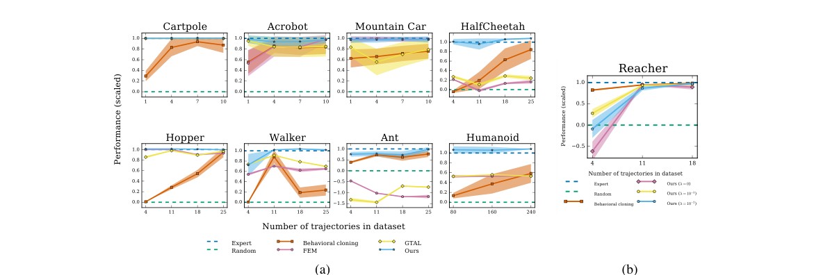
Figure 1: Performance of imitation learning algorithms across tasks and expert dataset sizes. (a) Classic control and MuJoCo results as reported in the paper.

图 1：各任务、各专家数据集规模下模仿学习算法的性能。（a）文中报告的经典控制与 MuJoCo 结果。

On the other MuJoCo environments, we saw a large performance boost for our algorithm over the baselines. Our algorithm almost always achieved at least 70% of expert performance for all dataset sizes we tested, nearly always dominating all the baselines. FEM and GTAL performed poorly for Ant, producing policies consistently worse than a policy that chooses actions uniformly at random. Behavioral cloning was able to reach satisfactory performance with enough data on HalfCheetah, Hopper, Walker, and Ant; but was unable to achieve more than 60% for Humanoid, on which our algorithm achieved exact expert performance for all tested dataset sizes.

在其余 MuJoCo 环境中，我们的算法相对基线有大幅提升。几乎对所有测试的数据集规模，它都能达到至少 70% 的专家性能，并几乎总是压过全部基线。FEM 与 GTAL 在 Ant 上很差，策略甚至持续差于均匀随机动作。行为克隆在 HalfCheetah、Hopper、Walker、Ant 上数据足够时可达到尚可的表现，但在 Humanoid 上无法超过 60%；而我们的算法在所有测试数据集规模上都达到了精确的专家性能。

7 Discussion and outlook

7 讨论与展望

As we demonstrated, our method is generally quite sample efficient in terms of expert data. However, it is not particularly sample efficient in terms of environment interaction during training. The number of such samples required to estimate the imitation objective gradient 18 was comparable to the number needed for TRPO to train the expert policies from reinforcement signals. We believe that we could significantly improve learning speed for our algorithm by initializing policy parameters with behavioral cloning, which requires no environment interaction at all.

如实验所示，我们的方法在专家数据上一般相当样本高效，但在训练期的环境交互上并不特别高效。估计模仿目标梯度 (18) 所需样本量，与用 TRPO 从强化信号训练专家策略所需量相当。我们相信：用行为克隆初始化策略参数（完全不需要环境交互）可以显著加快学习。

Fundamentally, our method is model free, so it will generally need more environment interaction than model-based methods. Guided cost learning [7], for instance, builds upon guided policy search [13] and inherits its sample efficiency, but also inherits its requirement that the model is well-approximated by iteratively fitted time-varying linear dynamics. Interestingly, both our Algorithm 1 and guided cost learning alternate between policy optimization steps and cost fitting (which we called discriminator fitting), even though the two algorithms are derived completely differently.

从根本上说，我们的方法是无模型的，因此一般会比基于模型的方法需要更多环境交互。例如 guided cost learning [7] 建立在 guided policy search [13] 之上，继承了其样本效率，也继承了「模型须被迭代拟合的时变线性动力学很好近似」的要求。有意思的是，算法 1 与 guided cost learning 都在策略优化与代价拟合（我们称作判别器拟合）之间交替，尽管两者推导路径完全不同。

Our approach builds upon a vast line of work on IRL [31, 1, 29, 28], and hence, just like IRL, our approach does not interact with the expert during training. Our method explores randomly to determine which actions bring a policy’s occupancy measure closer to the expert’s, whereas methods that do interact with the expert, like DAgger [24], can simply ask the expert for such actions. Ultimately, we believe that a method that combines well-chosen environment models with expert interaction will win in terms of sample complexity of both expert data and environment interaction.

我们的方法建立在漫长的 IRL 工作线之上 [31, 1, 29, 28]，因而也像 IRL 一样，训练时不与专家交互。我们的方法靠随机探索来判断哪些动作能让策略占用测度更接近专家；而像 DAgger [24] 这类会与专家交互的方法，可以直接向专家要这些动作。最终我们相信：把选得好的环境模型与专家交互结合起来的方法，会在专家数据与环境交互两方面的样本复杂度上胜出。

Acknowledgments

We thank Jayesh K. Gupta and John Schulman for assistance and advice. This work was supported by the SAIL-Toyota Center for AI Research, and by a NSF Graduate Research Fellowship (grant no. DGE-114747).

致谢

感谢 Jayesh K. Gupta 与 John Schulman 的协助与建议。本工作得到 SAIL-Toyota AI 研究中心以及 NSF 研究生研究奖学金（编号 DGE-114747）支持。

References

参考文献

Abbeel and Ng [2004] P. Abbeel and A. Y. Ng. Apprenticeship learning via inverse reinforcement learning. In Proceedings of the 21st International Conference on Machine Learning , 2004.

Barto et al. [1983] A. G. Barto, R. S. Sutton, and C. W. Anderson. Neuronlike adaptive elements that can solve difficult learning control problems. Systems, Man and Cybernetics, IEEE Transactions on , (5):834–846, 1983.

Bloem and Bambos [2014] M. Bloem and N. Bambos. Infinite time horizon maximum causal entropy inverse reinforcement learning. In Decision and Control (CDC), 2014 IEEE 53rd Annual Conference on , pages 4911–4916. IEEE, 2014.

Boyd and Vandenberghe [2004] S. Boyd and L. Vandenberghe. Convex optimization . Cambridge university press, 2004.

Brockman et al. [2016] G. Brockman, V. Cheung, L. Pettersson, J. Schneider, J. Schulman, J. Tang, and W. Zaremba. OpenAI Gym. arXiv preprint arXiv:1606.01540 , 2016.

Cover and Thomas [2012] T. M. Cover and J. A. Thomas. Elements of information theory . John Wiley & Sons, 2012.

Finn et al. [2016] C. Finn, S. Levine, and P. Abbeel. Guided cost learning: Deep inverse optimal control via policy optimization. In Proceedings of the 33rd International Conference on Machine Learning , 2016.

Geramifard et al. [2015] A. Geramifard, C. Dann, R. H. Klein, W. Dabney, and J. P. How. Rlpy: A value-function-based reinforcement learning framework for education and research. JMLR , 2015.

Goodfellow et al. [2014] I. Goodfellow, J. Pouget-Abadie, M. Mirza, B. Xu, D. Warde-Farley, S. Ozair, A. Courville, and Y. Bengio. Generative adversarial nets. In NIPS , pages 2672–2680, 2014.

Hiriart-Urruty and Lemaréchal [1996] J.-B. Hiriart-Urruty and C. Lemaréchal. Convex Analysis and Minimization Algorithms , volume 305. Springer, 1996.

Ho et al. [2016] J. Ho, J. K. Gupta, and S. Ermon. Model-free imitation learning with policy optimization. In Proceedings of the 33rd International Conference on Machine Learning , 2016.

Kingma and Ba [2014] D. Kingma and J. Ba. Adam: A method for stochastic optimization. arXiv preprint arXiv:1412.6980 , 2014.

Levine and Abbeel [2014] S. Levine and P. Abbeel. Learning neural network policies with guided policy search under unknown dynamics. In Advances in Neural Information Processing Systems , pages 1071–1079, 2014.

Levine and Koltun [2012] S. Levine and V. Koltun. Continuous inverse optimal control with locally optimal examples. In Proceedings of the 29th International Conference on Machine Learning , pages 41–48, 2012.

Levine et al. [2011] S. Levine, Z. Popovic, and V. Koltun. Nonlinear inverse reinforcement learning with gaussian processes. In Advances in Neural Information Processing Systems , pages 19–27, 2011.

Millar [1983] P. W. Millar. The minimax principle in asymptotic statistical theory. In Ecole d’Eté de Probabilités de Saint-Flour XI—1981 , pages 75–265. Springer, 1983.

Moore and Hall [1990] A. W. Moore and T. Hall. Efficient memory-based learning for robot control. 1990.

Ng and Russell [2000] A. Y. Ng and S. Russell. Algorithms for inverse reinforcement learning. In ICML , 2000.

Nguyen et al. [2009] X. Nguyen, M. J. Wainwright, and M. I. Jordan. On surrogate loss functions and f-divergences. The Annals of Statistics , pages 876–904, 2009.

Pomerleau [1991] D. A. Pomerleau. Efficient training of artificial neural networks for autonomous navigation. Neural Computation , 3(1):88–97, 1991.

Puterman [2014] M. L. Puterman. Markov decision processes: discrete stochastic dynamic programming . John Wiley & Sons, 2014.

Ratliff et al. [2009] N. D. Ratliff, D. Silver, and J. A. Bagnell. Learning to search: Functional gradient techniques for imitation learning. Autonomous Robots , 27(1):25–53, 2009.

Ross and Bagnell [2010] S. Ross and D. Bagnell. Efficient reductions for imitation learning. In AISTATS , pages 661–668, 2010.

Ross et al. [2011] S. Ross, G. J. Gordon, and D. Bagnell. A reduction of imitation learning and structured prediction to no-regret online learning. In AISTATS , pages 627–635, 2011.

Russell [1998] S. Russell. Learning agents for uncertain environments. In Proceedings of the Eleventh Annual Conference on Computational Learning Theory , pages 101–103. ACM, 1998.

Schulman et al. [2015a] J. Schulman, S. Levine, P. Abbeel, M. Jordan, and P. Moritz. Trust region policy optimization. In Proceedings of The 32nd International Conference on Machine Learning , pages 1889–1897, 2015a.

Schulman et al. [2015b] J. Schulman, P. Moritz, S. Levine, M. Jordan, and P. Abbeel. High-dimensional continuous control using generalized advantage estimation. arXiv preprint arXiv:1506.02438 , 2015b.

Syed and Schapire [2007] U. Syed and R. E. Schapire. A game-theoretic approach to apprenticeship learning. In Advances in Neural Information Processing Systems , pages 1449–1456, 2007.

Syed et al. [2008] U. Syed, M. Bowling, and R. E. Schapire. Apprenticeship learning using linear programming. In Proceedings of the 25th International Conference on Machine Learning , pages 1032–1039, 2008.

Todorov et al. [2012] E. Todorov, T. Erez, and Y. Tassa. Mujoco: A physics engine for model-based control. In Intelligent Robots and Systems (IROS), 2012 IEEE/RSJ International Conference on , pages 5026–5033. IEEE, 2012.

Ziebart et al. [2008] B. D. Ziebart, A. Maas, J. A. Bagnell, and A. K. Dey. Maximum entropy inverse reinforcement learning. In AAAI , AAAI’08, 2008.

Ziebart et al. [2010] B. D. Ziebart, J. A. Bagnell, and A. K. Dey. Modeling interaction via the principle of maximum causal entropy. In ICML , pages 1255–1262, 2010.

Appendix A Proofs

附录 A 证明

A.1 Proofs for Section 3

A.1 第 3 节的证明

Proof of Lemma 3.1.

First, we show strict concavity of $\bar{H}$. Let $\rho$ and $\rho^{\prime}$ be occupancy measures, and suppose $\lambda\in[0,1]$. For all $s$ and $a$, the log-sum inequality [6] implies:

引理 3.1 的证明。

先证 $\bar{H}$ 的严格凹性。令 $\rho$、$\rho^{\prime}$ 为占用测度，$\lambda\in[0,1]$。对所有 $s$、$a$，对数和不等式 [6] 给出：

$$\displaystyle- \\ \displaystyle(\lambda\rho(s,a)+(1-\lambda)\rho^{\prime}(s,a))\log\frac{\lambda\rho(s,a)+(1-\lambda)\rho^{\prime}(s,a)}{\sum_{a^{\prime}}(\lambda\rho(s,a^{\prime})+(1-\lambda)\rho^{\prime}(s,a^{\prime}))} \\ \displaystyle=-(\lambda\rho(s,a)+(1-\lambda)\rho^{\prime}(s,a))\log\frac{\lambda\rho(s,a)+(1-\lambda)\rho^{\prime}(s,a)}{\lambda\sum_{a^{\prime}}\rho(s,a^{\prime})+(1-\lambda)\sum_{a^{\prime}}\rho^{\prime}(s,a^{\prime})} \\ \displaystyle\geq-\lambda\rho(s,a)\log\frac{\lambda\rho(s,a)}{\lambda\sum_{a^{\prime}}\rho(s,a^{\prime})}-(1-\lambda)\rho^{\prime}(s,a)\log\frac{(1-\lambda)\rho^{\prime}(s,a)}{(1-\lambda)\sum_{a^{\prime}}\rho^{\prime}(s,a^{\prime})} \\ \displaystyle=\lambda\left(-\rho(s,a)\log\frac{\rho(s,a)}{\sum_{a^{\prime}}\rho(s,a^{\prime})}\right)+(1-\lambda)\left(-\rho^{\prime}(s,a)\log\frac{\rho^{\prime}(s,a)}{\sum_{a^{\prime}}\rho^{\prime}(s,a^{\prime})}\right), \tag{19}$$