FixMatch: Simplifying Semi-Supervised Learning with Consistency and Confidence
FixMatch: Simplifying Semi-Supervised Learning with Consistency and Confidence
FixMatch:用一致性和置信度简化半监督学习
34th Conference on Neural Information Processing Systems (NeurIPS 2020), Vancouver, Canada.
第34届神经信息处理系统会议(NeurIPS 2020),加拿大温哥华。
Abstract
摘要
Semi-supervised learning (SSL) provides an effective means of leveraging unlabeled data to improve a model's performance. This domain has seen fast progress recently, at the cost of requiring more complex methods. In this paper we propose FixMatch, an algorithm that is a significant simplification of existing SSL methods. FixMatch first generates pseudo-labels using the model's predictions on weakly-augmented unlabeled images. For a given image, the pseudo-label is only retained if the model produces a high-confidence prediction. The model is then trained to predict the pseudo-label when fed a strongly-augmented version of the same image. Despite its simplicity, we show that FixMatch achieves state-of-the-art performance across a variety of standard semi-supervised learning benchmarks, including 94.93% accuracy on CIFAR-10 with 250 labels and 88.61% accuracy with 40 – just 4 labels per class. We carry out an extensive ablation study to tease apart the experimental factors that are most important to FixMatch's success. The code is available at https://github.com/google-research/fixmatch .
半监督学习(SSL)能有效利用无标注数据来提升模型表现。这一方向近来进展很快,代价是方法变得越来越复杂。本文提出 FixMatch,它把已有 SSL 方法做了一次大幅简化。FixMatch 先用模型在弱增强无标注图像上的预测生成伪标签;只有当模型给出高置信度预测时,才保留这张图的伪标签。随后把同一张图的强增强版本送入模型,训练它去预测这个伪标签。尽管做法简单,FixMatch 在多项标准半监督基准上达到了当时的最好成绩,包括 CIFAR-10 在 250 个标签时准确率 94.93%,以及只用 40 个标签(每类仅 4 个)时准确率 88.61%。我们做了系统的消融实验,梳理对 FixMatch 成败最关键的实验因素。代码见 https://github.com/google-research/fixmatch 。
1 Introduction
1 引言
Deep neural networks have become the de facto model for computer vision applications. Their success is partially attributable to their scalability, i.e., the empirical observation that training them on larger datasets produces better performance [30, 20, 42, 55, 41, 21]. Deep networks often achieve their strong performance through supervised learning, which requires a labeled dataset. The performance benefit conferred by the use of a larger dataset can therefore come at a significant cost since labeling data often requires human labor. This cost can be particularly extreme when labeling must be done by an expert (for example, a doctor in medical applications).
深度神经网络已成为计算机视觉应用中的默认模型。它们的成功,部分来自可扩展性:在更大的数据集上训练,通常会得到更好的表现 [30, 20, 42, 55, 41, 21]。深度网络的强表现往往通过监督学习取得,而这需要带标注的数据集。因此,用更大规模数据换来的收益,常常伴随着高昂的标注成本,因为标注通常需要人工。当标注必须由专家完成时(例如医疗场景中的医生),这一成本会尤其突出。
A powerful approach for training models on a large amount of data without requiring a large amount of labels is semi-supervised learning (SSL). SSL mitigates the requirement for labeled data by providing a means of leveraging unlabeled data. Since unlabeled data can often be obtained with minimal human labor, any performance boost conferred by SSL often comes with low cost. This has led to a plethora of SSL methods that are designed for deep networks [33, 46, 24, 51, 4, 54, 3, 25, 45, 52].
若希望在大量数据上训练模型,却不必准备同样大量的标签,半监督学习(SSL)是一条有力的路。它通过利用无标注数据,减轻对标注数据的依赖。无标注数据往往只需很少人工就能收集,因此 SSL 带来的提升通常成本较低。这也催生了大量面向深度网络的 SSL 方法 [33, 46, 24, 51, 4, 54, 3, 25, 45, 52]。
A popular class of SSL methods can be viewed as producing an artificial label for unlabeled images and training the model to predict the artificial label when fed unlabeled images as input. For example, pseudo-labeling [25] (also called self-training [32, 55, 44, 47]) uses the model's class prediction as a label to train against. Similarly, consistency regularization [2, 46, 24] obtains an artificial label using the model's predicted distribution after randomly modifying the input or model function.
一类常见的 SSL 方法,可以看成是给无标注图像造出人工标签,再让模型在输入这些无标注图像时去预测该标签。例如,伪标签(pseudo-labeling)[25](也称自训练 [32, 55, 44, 47])直接把模型的类别预测当作训练标签。类似地,一致性正则 [2, 46, 24] 会在随机改动输入或模型函数之后,用模型的预测分布作为人工标签。
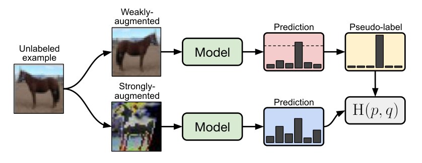
Figure 1: Diagram of FixMatch. A weakly-augmented image (top) is fed into the model to obtain predictions (red box). When the model assigns a probability to any class which is above a threshold (dotted line), the prediction is converted to a one-hot pseudo-label. Then, we compute the model's prediction for a strong augmentation of the same image (bottom). The model is trained to make its prediction on the strongly-augmented version match the pseudo-label via a cross-entropy loss.
图 1:FixMatch 示意图。弱增强图像(上)送入模型得到预测(红框)。当模型给某一类的概率超过阈值(虚线)时,该预测被转成独热伪标签。随后计算同一张图强增强版本的模型预测(下)。训练目标是让强增强版本上的预测通过交叉熵损失去对齐这个伪标签。
In this work, we break the trend of recent state-of-the-art methods that combine increasingly complex mechanisms [4, 54, 3] and produce a method that is simpler, but also more accurate. Our algorithm, FixMatch, produces artificial labels using both consistency regularization and pseudo-labeling. Crucially, the artificial label is produced based on a weakly-augmented unlabeled image (e.g., using only flip-and-shift data augmentation) which is used as a target when the model is fed a strongly-augmented version of the same image. Inspired by UDA [54] and ReMixMatch [3], we leverage Cutout [14], CTAugment [3], and RandAugment [11] for strong augmentation, which all produce heavily-distorted versions of a given image. Following the approach of pseudo-labeling [25], we only retain an artificial label if the model assigns a high probability to one of the possible classes. A diagram of FixMatch is shown in fig. 1.
近期不少领先方法把越来越复杂的机制叠在一起 [4, 54, 3]。本文想打破这一趋势,给出一种更简单、同时更准的方法。我们的算法 FixMatch 同时用一致性正则和伪标签来生成人工标签。关键在于:人工标签来自弱增强的无标注图像(例如只用翻转和平移),再把它当作目标,去监督同一张图的强增强版本。受 UDA [54] 和 ReMixMatch [3] 启发,强增强采用 Cutout [14]、CTAugment [3] 和 RandAugment [11],它们都会对图像做大幅度扭曲。沿用伪标签 [25] 的做法,只有当模型对某一类给出高概率时,我们才保留这个人工标签。FixMatch 的流程见图 1。
Despite its simplicity, we show that FixMatch obtains state-of-the-art performance on the most commonly-studied SSL benchmarks. For example, FixMatch achieves 94.93% accuracy on CIFAR-10 with 250 labeled examples compared to the previous state-of-the-art of 93.73% [3] in the standard experimental setting from [36]. We also explore the limits of our approach by applying it in the extremely-scarce-labels regime, obtaining 88.61% accuracy on CIFAR-10 with only 4 labels per class. Since FixMatch is a simplification of existing approaches but achieves substantially better performance, we include an extensive ablation study to determine which factors contribute the most to its success. A key benefit of FixMatch being a simplification of existing methods is that it requires many fewer additional hyperparameters. As such, it allows us to perform an extensive ablation study of each of them. Our ablation study also includes basic fully-supervised learning experimental choices that are often ignored or not reported when new SSL methods are proposed (such as the optimizer or learning rate schedule).
尽管简单,FixMatch 仍在最常研究的 SSL 基准上取得了当时最好的成绩。例如,在 [36] 的标准设定下,CIFAR-10 使用 250 个有标注样本时,FixMatch 准确率为 94.93%,此前最好结果是 93.73% [3]。我们还把它推到标签极少的情形:CIFAR-10 每类只有 4 个标签时,准确率仍有 88.61%。FixMatch 是对已有方法的简化,却明显更好,因此我们做了系统的消融,以弄清哪些因素贡献最大。它作为简化方法的另一个好处是额外超参数少得多,这让我们能够对每一个超参数做充分消融。消融里也包括优化器、学习率日程这类在提出新 SSL 方法时常常被忽略或不报告的、本属全监督训练的基本选择。
2 FixMatch
FixMatch is a combination of two approaches to SSL: Consistency regularization and pseudo-labeling. Its main novelty comes from the combination of these two ingredients as well as the use of a separate weak and strong augmentation when performing consistency regularization. In this section, we first review consistency regularization and pseudo-labeling before describing FixMatch in detail. We also describe the other factors, such as regularization, which contribute to FixMatch's empirical success.
FixMatch 把半监督里的两条路合在一起:一致性正则和伪标签。主要新意就在于这一组合,以及在做一致性正则时分别使用弱增强和强增强。本节先回顾一致性正则和伪标签,再详细介绍 FixMatch,并说明正则化等对其经验表现同样重要的其他因素。
For an -class classification problem, let be a batch of labeled examples, where are the training examples and are one-hot labels. Let be a batch of unlabeled examples where is a hyperparameter that determines the relative sizes of and . Let be the predicted class distribution produced by the model for input . We denote the cross-entropy between two probability distributions and as . We perform two types of augmentations as part of FixMatch: strong and weak, denoted by and respectively. We describe the form of augmentation we use for and in section 2.3.
对一个 类分类问题,记 为大小 的有标注批次,其中 是训练样本, 是独热标签。记 为大小 的无标注批次,超参数 控制 与 的相对规模。 表示模型对输入 给出的预测类别分布。两个概率分布 与 之间的交叉熵记为 。FixMatch 使用两类增强:强增强 与弱增强 ,具体形式在 2.3 节说明。
2.1 Background
2.1 背景
Consistency regularization is an important component of recent state-of-the-art SSL algorithms. Consistency regularization utilizes unlabeled data by relying on the assumption that the model should output similar predictions when fed perturbed versions of the same image. This idea was first proposed in [2] and popularized by [46, 24], where the model is trained both via a standard supervised classification loss and on unlabeled data via the loss function
一致性正则是近期不少领先 SSL 算法的重要组成部分。它利用无标注数据,依据的假设是:同一张图的不同扰动版本,模型应给出相近的预测。这一想法最早见于 [2],并由 [46, 24] 推广:模型既用标准的有监督分类损失训练,也对无标注数据使用如下损失
Note that both and are stochastic functions, so the two terms in eq. (1) will indeed have different values. Extensions to this idea include using an adversarial transformation in place of [33], using a running average or past model predictions for one invocation of [51, 24], using a cross-entropy loss in place of the squared loss [33, 54, 3], using stronger forms of augmentation [54, 3], and using consistency regularization as a component in a larger SSL pipeline [4, 3].
注意 和 都是随机函数,因此式 (1) 中的两项取值确实会不同。后续扩展包括:用对抗变换代替 [33];在一次 调用中使用参数的滑动平均或历史模型预测 [51, 24];用交叉熵代替平方 损失 [33, 54, 3];采用更强的增强 [54, 3];以及把一致性正则放进更大的 SSL 流程中 [4, 3]。
Pseudo-labeling leverages the idea of using the model itself to obtain artificial labels for unlabeled data [32, 47]. Specifically, this refers to the use of “hard” labels (i.e., the of the model's output) and only retaining artificial labels whose largest class probability fall above a predefined threshold [25]. Letting , pseudo-labeling uses the following loss function:
伪标签的想法是用模型自身为无标注数据生成人工标签 [32, 47]。具体来说,这里指使用“硬”标签(即模型输出的 ),并且只保留最大类概率超过预定阈值的那些人工标签 [25]。记 ,伪标签使用如下损失:
where and is the threshold. For simplicity, we assume that applied to a probability distribution produces a valid “one-hot” probability distribution. The use of a hard label makes pseudo-labeling closely related to entropy minimization [17, 45], where the model's predictions are encouraged to be low-entropy (i.e., high-confidence) on unlabeled data.
其中 , 是阈值。为简单起见,我们假定对概率分布做 会得到合法的独热分布。使用硬标签使伪标签与熵最小化 [17, 45] 密切相关:后者鼓励模型在无标注数据上给出低熵(即高置信度)的预测。
2.2 Our Algorithm: FixMatch
2.2 我们的算法:FixMatch
The loss function for FixMatch consists of two cross-entropy loss terms: a supervised loss applied to labeled data and an unsupervised loss . Specifically, is just the standard cross-entropy loss on weakly augmented labeled examples:
FixMatch 的损失函数由两项交叉熵组成:作用在有标注数据上的监督损失 ,以及无监督损失 。其中 就是弱增强有标注样本上的标准交叉熵:
FixMatch computes an artificial label for each unlabeled example which is then used in a standard cross-entropy loss. To obtain an artificial label, we first compute the model's predicted class distribution given a weakly-augmented version of a given unlabeled image: . Then, we use as a pseudo-label, except we enforce the cross-entropy loss against the model's output for a strongly-augmented version of :
FixMatch 为每个无标注样本计算一个人造标签,再把它用进标准交叉熵损失。具体做法是:先对无标注图像做弱增强,计算模型的预测类别分布 ;再取 作为伪标签,但交叉熵是加在同一张图 的强增强版本上的模型输出上:
In practice, we include all labeled data as part of unlabeled data without their labels when constructing .
实际构造 时,我们会把全部有标注数据去掉标签后一并纳入无标注数据。
where is a scalar hyperparameter denoting the threshold above which we retain a pseudo-label. The loss minimized by FixMatch is simply where is a fixed scalar hyperparameter denoting the relative weight of the unlabeled loss. We present a complete algorithm for FixMatch in algorithm 1 of the supplementary material.
其中 是标量超参数,表示保留伪标签的置信度阈值。FixMatch 最小化的损失就是 ,其中 是固定的标量超参数,表示无标注损失的相对权重。完整算法见补充材料中的算法 1。
While eq. (4) is similar to the pseudo-labeling loss in eq. (2), it is crucially different in that the artificial label is computed based on a weakly-augmented image and the loss is enforced against the model's output for a strongly-augmented image. This introduces a form of consistency regularization which, as we will show in section 5, is crucial to FixMatch's success. We also note that it is typical in modern SSL algorithms to increase the weight of the unlabeled loss term () during training [51, 24, 4, 3, 36]. We found that this was unnecessary for FixMatch, which may be due to the fact that is typically less than early in training. As training progresses, the model's predictions become more confident and it is more frequently the case that . This suggests that pseudo-labeling may produce a natural curriculum “for free”. Similar justifications have been used in the past for ignoring low-confidence predictions in visual domain adaptation [15].
式 (4) 与式 (2) 中的伪标签损失相近,但关键不同在于:人工标签来自弱增强图像,损失却加在强增强图像的模型输出上。这就引入了一种一致性正则;第 5 节会表明,这对 FixMatch 的成功至关重要。另外,现代 SSL 算法通常会在训练过程中逐步加大无标注损失的权重 [51, 24, 4, 3, 36]。我们发现 FixMatch 不必这样做,原因可能是训练早期 往往低于 。随着训练进行,模型预测更有把握, 的情形也更频繁。这意味着伪标签或许能“免费”形成一个自然的课程安排。视觉域适应里忽略低置信度预测,也曾给出过类似理由 [15]。
2.3 Augmentation in FixMatch
2.3 FixMatch 中的数据增强
FixMatch leverages two kinds of augmentations: “weak” and “strong”. In all of our experiments, weak augmentation is a standard flip-and-shift augmentation strategy. Specifically, we randomly flip images horizontally with a probability of 50% on all datasets except SVHN and we randomly translate images by up to 12.5% vertically and horizontally.
FixMatch 使用两类增强:“弱”和“强”。在全部实验中,弱增强就是标准的翻转和平移:除 SVHN 外,所有数据集都以 50% 的概率做水平翻转,并在垂直和水平方向上随机平移最多 12.5%。
For “strong” augmentation, we experiment with two methods based on AutoAugment [10], which are then followed by the Cutout [14]. AutoAugment uses reinforcement learning to find an augmentation strategy comprising transformations from the Python Imaging Library. This requires labeled data to learn the augmentation strategy, making it problematic to use in SSL settings where limited labeled data is available. As a result, variants of AutoAugment which do not require the augmentation strategy to be learned ahead of time with labeled data, such as RandAugment [11] and CTAugment [3], have been proposed. Instead of using a learned strategy, both RandAugment and CTAugment randomly select transformations for each sample. For RandAugment, the magnitude that controls the severity of all distortions is randomly sampled from a pre-defined range (RandAugment with random magnitude was also used for UDA by [54]), whereas the magnitudes of individual transformations are learned on-the-fly for CTAugment. Refer to appendix E for more details.
强增强方面,我们试验了两种基于 AutoAugment [10] 的方法,并在其后接上 Cutout [14]。AutoAugment 用强化学习,从 Python Imaging Library 的变换中搜索增强策略。这需要有标注数据来学习策略,在标注有限的 SSL 设定里并不合适。因此出现了不必事先用有标注数据学好策略的变体,例如 RandAugment [11] 和 CTAugment [3]。它们不再使用预先学好的策略,而是对每个样本随机选择变换。RandAugment 中控制所有扭曲强度的幅度,会从一个预定义区间里随机采样([54] 在 UDA 里也用过带随机幅度的 RandAugment);CTAugment 则在训练过程中在线学习各个变换的幅度。更多细节见附录 E。
2.4 Additional important factors
2.4 其他重要因素
Semi-supervised performance can be substantially impacted by factors other than the SSL algorithm used because considerations like the amount of regularization can be particularly important in the low-label regime. This is compounded by the fact that the performance of deep networks trained for image classification can heavily depend on the architecture, optimizer, training schedule, etc. These factors are typically not emphasized when new SSL algorithms are introduced. Instead, we endeavor to quantify their importance and highlight which ones have a significant impact on performance. Most analysis is performed in section 5. In this section we identify a few key considerations.
半监督表现会受到 SSL 算法以外许多因素的显著影响,因为在少标签情形下,正则强度之类的选择往往特别重要。再加上图像分类深度网络的表现又高度依赖架构、优化器、训练日程等。提出新的 SSL 算法时,这些因素通常不被强调。我们则试图量化它们的重要性,并指出哪些选择对表现影响显著。主要分析放在第 5 节,本节先点出几项关键考虑。
First, as mentioned above, we find that regularization is particularly important. In all of our models and experiments, we use simple weight decay regularization. We also found that using the Adam optimizer [22] resulted in worse performance and instead use standard SGD with momentum [50, 40, 34]. We did not find a substantial difference between standard and Nesterov momentum. For a learning rate schedule, we use a cosine learning rate decay [28] which sets the learning rate to where is the initial learning rate, is the current training step, and is the total number of training steps. Finally, we report final performance using an exponential moving average of model parameters.
首先,如前所述,正则化特别重要。全部模型与实验都使用简单的权重衰减。我们还发现 Adam 优化器 [22] 效果较差,因而改用带动量的标准 SGD [50, 40, 34]。标准动量与 Nesterov 动量之间没有实质差别。学习率日程采用余弦衰减 [28],把学习率设为 ,其中 是初始学习率, 是当前训练步数, 是总训练步数。最终表现按模型参数的指数滑动平均来报告。
2.5 Extensions of FixMatch
2.5 FixMatch 的扩展
Due to its simplicity, FixMatch can be readily extended with techniques in SSL literature. For example, both Augmentation Anchoring (where strong augmentations are used for consistency regularization for each unlabeled example) and Distribution Alignment (which encourages the model predictions to have the same class distribution as the labeled set) from ReMixMatch [3] can be straightforwardly applied to FixMatch. Moreover, one may replace strong augmentations in FixMatch with modality-agnostic augmentation strategies, such as MixUp [59] or adversarial perturbations [33]. We present some exploration and experiments with these extensions in appendix D.
正因为简单,FixMatch 很容易接上 SSL 文献中的其他技术。例如,ReMixMatch [3] 中的增强锚定(Augmentation Anchoring,对每个无标注样本使用 次强增强做一致性正则)和分布对齐(Distribution Alignment,鼓励模型预测的类别分布与有标注集合一致),都可以直接接到 FixMatch 上。此外,也可以把其中的强增强替换成与模态无关的策略,例如 MixUp [59] 或对抗扰动 [33]。这些扩展的探索和实验见附录 D。
3 Related work
3 相关工作
Semi-supervised learning is a mature field with a huge diversity of approaches. In this review, we focus on methods closely related to FixMatch. Broader introductions are provided in [60, 61, 6].
半监督学习已是一个方法极其多样的成熟领域。本节评述聚焦与 FixMatch 密切相关的方法。更全面的介绍见 [60, 61, 6]。
The idea behind self-training has been around for decades [47, 32]. The generality of self-training (i.e., using a model's predictions to obtain artificial labels for unlabeled data) has led it to be applied in many domains including NLP [31], object detection [44], image classification [25, 55], domain adaptation [62], to name a few. Pseudo-labeling refers to a specific variant where model predictions are converted to hard labels [25], which is often used along with a confidence-based thresholding that retains unlabeled examples only when the classifier is sufficiently confident (e.g., [44]). While some studies have suggested that pseudo-labeling is not competitive against other modern SSL algorithms on its own [36], recent SSL algorithms have used pseudo-labeling as a part of their pipeline to produce better results [1, 39]. As mentioned above, pseudo-labeling results in a form of entropy minimization [17] which has been used as a component for many SSL techniques [33].
自训练的想法已有数十年历史 [47, 32]。正因为它足够通用(用模型预测为无标注数据生成人工标签),它被用到许多领域,包括自然语言处理 [31]、目标检测 [44]、图像分类 [25, 55]、域适应 [62] 等。伪标签指其中一种具体做法:把模型预测转成硬标签 [25],并常常配合基于置信度的阈值,只在分类器足够有把握时才保留该无标注样本(例如 [44])。虽有研究认为,单用伪标签并不足以抗衡其他现代 SSL 算法 [36],但近期一些 SSL 算法仍把它作为流程的一部分,并据此得到更好结果 [1, 39]。如前所述,伪标签会带来一种熵最小化 [17],而熵最小化本身也是许多 SSL 技术的组成元件 [33]。
Consistency regularization was first proposed by [2] and later referred to as “Transformation/Stability” (or TS for short) [46] or the “Π-Model” [43]. Early extensions included using an exponential moving average of model parameters [51] or using previous model checkpoints [24] when producing artificial labels. Several methods have been used to produce random perturbations including data augmentation [15], stochastic regularization (e.g. Dropout [49]) [46, 24], and adversarial perturbations [33]. More recently, it has been shown that using strong data augmentation can produce better results [54, 3]. These heavily-augmented examples are almost certainly outside of the data distribution, which has in fact been shown to be beneficial for SSL [12]. Noisy Student [55] has integrated these techniques into a self-training framework and demonstrated impressive performance on ImageNet with additional massive amount of unlabeled data.
一致性正则最早由 [2] 提出,后来被称为“变换/稳定性”(Transformation/Stability,简称 TS)[46] 或“Π-Model”[43]。早期扩展包括:生成人工标签时使用模型参数的指数滑动平均 [51],或使用先前的模型检查点 [24]。产生随机扰动的方式有多种,包括数据增强 [15]、随机正则(如 Dropout [49])[46, 24],以及对抗扰动 [33]。近来有工作表明,使用强数据增强能得到更好结果 [54, 3]。这些被大幅增强的样本几乎肯定落在数据分布之外,而这对 SSL 其实是有益的 [12]。Noisy Student [55] 把这些技术纳入自训练框架,并在 ImageNet 上借助海量额外无标注数据取得了出色表现。
Of the aforementioned work, FixMatch bears the closest resemblance to two recent methods: Unsupervised Data Augmentation (UDA) [54] and ReMixMatch [3]. They both use a weakly-augmented example to generate an artificial label and enforce consistency against strongly-augmented examples. Neither of them uses pseudo-labeling, but both approaches “sharpen” the artificial label to encourage the model to produce high-confidence predictions. UDA in particular also only enforces consistency when the highest probability in the predicted class distribution for the artificial label is above a threshold. The thresholded pseudo-labeling of FixMatch has a similar effect to sharpening. In addition, ReMixMatch anneals the weight of the unlabeled data loss, which we omit from FixMatch because we posit that the thresholding used in pseudo-labeling has a similar effect (as mentioned in section 2.2). These similarities suggest that FixMatch can be viewed as a substantially simplified version of UDA and ReMixMatch, where we have combined two common techniques (pseudo-labeling and consistency regularization) while removing many components (sharpening, training signal annealing from UDA, distribution alignment and the rotation loss from ReMixMatch, etc.).
在上述工作中,与 FixMatch 最接近的是两个近期方法:无监督数据增强(UDA)[54] 和 ReMixMatch [3]。它们都用弱增强样本生成人工标签,再对强增强样本施加一致性约束。两者都不使用伪标签,而是对人工标签做“锐化”(sharpen),以鼓励模型给出高置信度预测。UDA 还规定:只有当人工标签对应的预测分布中最大概率超过阈值时,才施加一致性。FixMatch 带阈值的伪标签,效果与锐化相近。此外,ReMixMatch 会逐步调整无标注损失的权重;FixMatch 去掉了这一项,因为我们推测伪标签中的阈值已经有类似作用(见 2.2 节)。这些相似之处表明,可以把 FixMatch 看成 UDA 和 ReMixMatch 的大幅简化版:它组合了伪标签和一致性正则这两项常用技术,同时去掉了许多组件(锐化、UDA 中的训练信号退火、ReMixMatch 中的分布对齐和旋转损失等)。
Since the core of FixMatch is a simple combination of two existing techniques, it also bears substantial similarities to many previously-proposed SSL algorithms. We provide a concise comparison of each of these techniques in table 1 where we list the augmentation used for the artificial label, the model's prediction, and any post-processing applied to the artificial label. A more thorough comparison of these different algorithms and their constituent approaches is provided in the following section.
FixMatch 的核心只是两种已有技术的简单组合,因此它与许多先前提出的 SSL 算法也颇为相似。表 1 对这些方法做了扼要对照,列出了人工标签所用的增强、模型预测所用的增强,以及对人工标签的后处理。下一节会更系统地比较这些算法及其组成模块。
| Algorithm | Artificial label augmentation | Prediction augmentation | Artificial label post-processing | Notes |
|---|---|---|---|---|
| TS / Π-Model | Weak | Weak | None | |
| Temporal Ensembling | Weak | Weak | None | Uses model from earlier in training |
| Mean Teacher | Weak | Weak | None | Uses an EMA of parameters |
| Virtual Adversarial Training | None | Adversarial | None | |
| UDA | Weak | Strong | Sharpening | Ignores low-confidence artificial labels |
| MixMatch | Weak | Weak | Sharpening | Averages multiple artificial labels |
| ReMixMatch | Weak | Strong | Sharpening | Sums losses for multiple predictions |
| FixMatch | Weak | Strong | Pseudo-labeling |
Table 1: Comparison of SSL algorithms which include a form of consistency regularization and which (optionally) apply some form of post-processing to the artificial labels. We only mention those components of the SSL algorithm relevant to producing the artificial labels (for example, Virtual Adversarial Training additionally uses entropy minimization [17], MixMatch and ReMixMatch also use MixUp [59], UDA includes additional techniques like training signal annealing, etc.).
| 算法 | 人工标签所用增强 | 预测所用增强 | 人工标签后处理 | 备注 |
|---|---|---|---|---|
| TS / Π-Model | 弱 | 弱 | 无 | |
| Temporal Ensembling | 弱 | 弱 | 无 | 使用训练更早阶段的模型 |
| Mean Teacher | 弱 | 弱 | 无 | 使用参数的指数滑动平均 |
| Virtual Adversarial Training | 无 | 对抗 | 无 | |
| UDA | 弱 | 强 | 锐化 | 忽略低置信度人工标签 |
| MixMatch | 弱 | 弱 | 锐化 | 对多个人工标签取平均 |
| ReMixMatch | 弱 | 强 | 锐化 | 对多次预测的损失求和 |
| FixMatch | 弱 | 强 | 伪标签 |
表 1:对包含某种一致性正则、并(可选地)对人工标签做某种后处理的 SSL 算法的比较。这里只列出与生成人工标签相关的部分(例如,Virtual Adversarial Training 另外使用了熵最小化 [17],MixMatch 和 ReMixMatch 还使用了 MixUp [59],UDA 还包括训练信号退火等技术)。
4 Experiments
4 实验
We evaluate the efficacy of FixMatch on several SSL image classification benchmarks. Specifically, we perform experiments with varying amounts of labeled data and augmentation strategies on CIFAR-10/100 [23], SVHN [35], STL-10 [9], and ImageNet [13], following standard SSL evaluation protocols [36, 4, 3]. In many cases, we perform experiments with fewer labels than previously considered since FixMatch shows promise in extremely label-scarce settings. Note that we use an identical set of hyperparameters (, , , , , , ) across all amounts of labeled examples and datasets other than ImageNet. A complete list of hyperparameters is reported in appendix B.1. We include an extensive ablation study in section 5 to tease apart the importance of the different components and hyperparameters of FixMatch, including factors that are not explicitly part of the SSL algorithm such as the optimizer and learning rate.
我们在多个半监督图像分类基准上检验 FixMatch。具体来说,我们在 CIFAR-10/100 [23]、SVHN [35]、STL-10 [9] 和 ImageNet [13] 上,按照标准 SSL 评测协议 [36, 4, 3],改变有标注数量和增强策略进行实验。由于 FixMatch 在标签极度稀缺时仍有潜力,许多实验使用的标签数比以往工作更少。除 ImageNet 外,所有有标注数量和数据集都使用同一组超参数(,,,,,,)。完整超参数列表见附录 B.1。第 5 节有系统的消融,用以分离 FixMatch 各组件和超参数的重要性,也包括优化器和学习率这类并不属于 SSL 算法本身的因素。
refers to a momentum in SGD optimizer. The definition of other hyperparameters are found in section 2.
指 SGD 优化器中的动量。其余超参数的定义见第 2 节。
| Method | CIFAR-10 40 labels | CIFAR-10 250 labels | CIFAR-10 4000 labels | CIFAR-100 400 labels | CIFAR-100 2500 labels | CIFAR-100 10000 labels | SVHN 40 labels | SVHN 250 labels | SVHN 1000 labels | STL-10 1000 labels |
|---|---|---|---|---|---|---|---|---|---|---|
| Π-Model | – | – | – | |||||||
| Pseudo-Labeling | – | – | – | |||||||
| Mean Teacher | – | – | – | |||||||
| MixMatch | ||||||||||
| UDA | ||||||||||
| ReMixMatch | ||||||||||
| FixMatch (RA) | ||||||||||
| FixMatch (CTA) |
Table 2: Error rates for CIFAR-10, CIFAR-100, SVHN and STL-10 on 5 different folds. FixMatch (RA) uses RandAugment [11] and FixMatch (CTA) uses CTAugment [3] for strong-augmentation. All baseline models (Π-Model [43], Pseudo-Labeling [25], Mean Teacher [51], MixMatch [4], UDA [54], and ReMixMatch [3]) are tested using the same codebase.
| 方法 | CIFAR-10 40 标签 | CIFAR-10 250 标签 | CIFAR-10 4000 标签 | CIFAR-100 400 标签 | CIFAR-100 2500 标签 | CIFAR-100 10000 标签 | SVHN 40 标签 | SVHN 250 标签 | SVHN 1000 标签 | STL-10 1000 标签 |
|---|---|---|---|---|---|---|---|---|---|---|
| Π-Model | – | – | – | |||||||
| Pseudo-Labeling | – | – | – | |||||||
| Mean Teacher | – | – | – | |||||||
| MixMatch | ||||||||||
| UDA | ||||||||||
| ReMixMatch | ||||||||||
| FixMatch (RA) | ||||||||||
| FixMatch (CTA) |
表 2:CIFAR-10、CIFAR-100、SVHN 和 STL-10 在 5 个不同折上的错误率。FixMatch (RA) 的强增强使用 RandAugment [11],FixMatch (CTA) 使用 CTAugment [3]。所有基线(Π-Model [43]、Pseudo-Labeling [25]、Mean Teacher [51]、MixMatch [4]、UDA [54] 和 ReMixMatch [3])都在同一套代码库上测试。
4.1 CIFAR-10, CIFAR-100, and SVHN
4.1 CIFAR-10、CIFAR-100 和 SVHN
We compare FixMatch to various existing methods on the standard CIFAR-10, CIFAR-100, and SVHN benchmarks. As suggested by [36], we reimplemented all existing baselines and performed all experiments using the same codebase. In particular, we use the same network architecture and training protocol, including the optimizer, learning rate schedule, data preprocessing, etc. across all SSL methods. Following [4], we used a Wide ResNet-28-2 [56] with 1.5M parameters for CIFAR-10 and SVHN, WRN-28-8 for CIFAR-100, and WRN-37-2 for STL-10. For baselines, we consider methods that are similar to FixMatch and/or are state-of-the-art: Π-Model [43], Mean Teacher [51], Pseudo-Label [25], MixMatch [4], UDA [54], and ReMixMatch [3]. Besides [3], previous work has not considered fewer than 25 labels per class on these benchmarks. Performing better with less supervision is the central goal of SSL in practice since it alleviates the need for labeled data. We also consider the setting where only 4 labeled images are given for each class on each dataset. As far as we are aware, we are the first to run any experiments at 4 labels per class on CIFAR-100.
我们在标准的 CIFAR-10、CIFAR-100 和 SVHN 基准上,把 FixMatch 与多种已有方法比较。按 [36] 的建议,我们重实现了全部已有基线,并在同一套代码库上完成所有实验。尤其是,所有 SSL 方法使用相同的网络架构和训练协议,包括优化器、学习率日程、数据预处理等。遵循 [4],CIFAR-10 和 SVHN 使用 150 万参数的 Wide ResNet-28-2 [56],CIFAR-100 使用 WRN-28-8,STL-10 使用 WRN-37-2。基线方面,我们选择与 FixMatch 相近和/或当时领先的方法:Π-Model [43]、Mean Teacher [51]、Pseudo-Label [25]、MixMatch [4]、UDA [54] 和 ReMixMatch [3]。除 [3] 外,以往工作在这些基准上从未考虑每类少于 25 个标签的设定。用更少监督取得更好结果,正是 SSL 在实践中的核心目标,因为它能减轻对标注数据的依赖。我们还考虑了每个数据集每类只有 4 张有标注图像的设定。据我们所知,这是首次在 CIFAR-100 上做每类 4 个标签的实验。
We report the performance of all baselines along with FixMatch in table 2. We compute the mean and variance of accuracy when training on 5 different “folds” of labeled data. We omit results with 4 labels per class for Π-Model, Mean Teacher, and Pseudo-Labeling since the performance was poor at 250 labels. MixMatch, ReMixMatch, and UDA all perform reasonably well with 40 and 250 labels, but we find that FixMatch substantially outperforms each of these methods while nevertheless being simpler. For example, FixMatch achieves an average error rate of 11.39% on CIFAR-10 with 4 labels per class. As a point of reference, among the methods studied in [36] (where the same network architecture was used), the lowest error rate achieved on CIFAR-10 with 400 labels per class was 13.13%. Our results also compare favorably to recent state-of-the-art results achieved by ReMixMatch [3], despite the fact that we omit various components such as the self-supervised loss. Our results are state-of-the-art on all datasets except for CIFAR-100 where ReMixMatch performs a bit better. To understand why ReMixMatch performs better than FixMatch, we experimented with a few variants of FixMatch which copy various components of ReMixMatch into FixMatch. We find that the most important term is Distribution Alignment (DA), which encourages the model predictions to have the same class distribution as the labeled set. Combining FixMatch with DA reaches a 40.14% error rate with 400 labeled examples, which is substantially better than the 44.28% achieved by ReMixMatch.
表 2 报告了全部基线与 FixMatch 的表现。我们在 5 个不同的有标注数据“折”上训练,并计算准确率的均值与方差。Π-Model、Mean Teacher 和 Pseudo-Labeling 在 250 个标签时已经表现较差,因此省略了每类 4 个标签的结果。MixMatch、ReMixMatch 和 UDA 在 40 和 250 个标签时都还过得去,但 FixMatch 在更简单的同时明显超过了它们。例如,CIFAR-10 每类 4 个标签时,FixMatch 的平均错误率是 11.39%。作为对照,[36] 所研究的方法(使用相同网络架构)在 CIFAR-10 每类 400 个标签时,最低错误率也有 13.13%。与 ReMixMatch [3] 当时的领先结果相比,我们的成绩同样有利,尽管我们去掉了自监督损失等组件。除 CIFAR-100 上 ReMixMatch 略好之外,我们在所有数据集上都取得了当时最好的结果。为理解 ReMixMatch 为何在 CIFAR-100 上更好,我们把 ReMixMatch 的若干组件搬进 FixMatch 做了变体实验。最重要的一项是分布对齐(DA),它鼓励模型预测的类别分布与有标注集合一致。FixMatch 加上 DA 后,在 400 个有标注样本上错误率达到 40.14%,明显优于 ReMixMatch 的 44.28%。
We find that in most cases the performance of FixMatch using CTAugment and RandAugment is similar, except in the settings where we have 4 labels per class. This may be explained by the fact that these results are particularly high-variance. For example, the variance over 5 different folds for CIFAR-10 with 4 labels per class is 3.35%, which is significantly higher than that with 25 labels per class (0.33%). The error rates are also affected significantly by the random seeds when the number of labeled examples per class is extremely small, as shown in table 8 of supplementary material.
多数情况下,FixMatch 使用 CTAugment 与使用 RandAugment 的表现相近,例外是每类只有 4 个标签的设定。这可能是因为这些结果的方差特别大。例如,CIFAR-10 每类 4 个标签时,5 折之间的标准差是 3.35%,远高于每类 25 个标签时的 0.33%。当每类有标注样本极少时,随机种子也会显著影响错误率,补充材料的表 8 给出了结果。

Figure 2: FixMatch reaches 78% CIFAR-10 accuracy using only above 10 labeled images.
图 2:FixMatch 仅用上面这 10 张有标注图像,就在 CIFAR-10 上达到 78% 准确率。
4.2 STL-10
The STL-10 dataset contains 5,000 labeled images of size from 10 classes and 100,000 unlabeled images. There exist out-of-distribution images in the unlabeled set, making it a more realistic and challenging test of SSL performance. We test SSL algorithms on five of the predefined folds of 1,000 labeled images each. Following [4], we use a WRN-37-2 network (comprising 5.9M parameters). As in table 2, FixMatch achieves the state-of-the-art performance of ReMixMatch [3] despite being significantly simpler.
STL-10 数据集包含 10 类、大小为 的 5,000 张有标注图像,以及 100,000 张无标注图像。无标注集合中存在分布外图像,因而更能检验 SSL 在真实、更有挑战的条件下的表现。我们在预先划分的 5 折上测试,每折 1,000 张有标注图像。遵循 [4],使用含 590 万参数的 WRN-37-2。如表 2 所示,FixMatch 达到了与 ReMixMatch [3] 相当的最好成绩,但要简单得多。
We clarify that both FixMatch and ReMixMatch [3], which has reported an incorrect number of network parameters (23.8M), are tested with the same network architecture containing 5.9M parameters.
需说明的是,ReMixMatch [3] 曾把网络参数量误报为 2380 万;FixMatch 与 ReMixMatch 实际都在同一含 590 万参数的网络架构上测试。
4.3 ImageNet
We evaluate FixMatch on ImageNet to verify that it performs well on a larger and more complex dataset. Following [54], we use 10% of the training data as labeled and treat the rest as unlabeled examples. We use a ResNet-50 network architecture and RandAugment [11] as strong augmentation for this experiment. We include additional implementation details in appendix C. FixMatch achieves a top-1 error rate of , which is 2.68% better than UDA [54]. Our top-5 error rate is . While S4L [57] holds state-of-the-art on semi-supervised ImageNet with a 26.79% error rate, it leverages 2 additional training phases (pseudo-label re-training and supervised fine-tuning) to significantly lower the error rate from 30.27% after the first phase. FixMatch outperforms S4L after its first phase, and it is possible that a similar performance gain could be achieved by incorporating these techniques into FixMatch.
为确认 FixMatch 在更大、更复杂的数据集上同样有效,我们在 ImageNet 上做了评测。遵循 [54],用 10% 的训练数据作为有标注,其余当作无标注。该实验使用 ResNet-50 架构,强增强为 RandAugment [11]。更多实现细节见附录 C。FixMatch 的 top-1 错误率为 ,比 UDA [54] 低 2.68%;top-5 错误率为 。半监督 ImageNet 上当时最好的是 S4L [57] 的 26.79% 错误率,但它额外使用了两个训练阶段(用伪标签再训练和有监督微调),把第一阶段结束后的 30.27% 大幅压了下去。FixMatch 已经超过 S4L 第一阶段的结果;若把这些技术接到 FixMatch 上,或许也能获得类似提升。
4.4 Barely Supervised Learning
4.4 极少监督学习
To test the limits of our proposed approach, we applied FixMatch to CIFAR-10 with only one example per class. We conduct two sets of experiments.
为了测试方法的极限,我们把 FixMatch 用到 CIFAR-10 上、每类只有一个样本的设定。我们做了两组实验。
The experimental protocol of barely supervised learning (BSL) shares similarities to those of few-shot learning (FSL) [37] as they both assume a limited availability (e.g., 1 or 5) of labeled examples from categories of interest. However, two protocols have a critical difference, where for FSL one is provided with extra labeled training examples from regular classes, whereas for BSL one is given additional unlabeled training examples.
极少监督学习(BSL)的实验设定与少样本学习(FSL)[37] 有相似之处,二者都假定感兴趣类别只有很少(例如 1 或 5 个)有标注样本。但有一个关键差别:FSL 还会提供来自常规类别的额外有标注训练样本,而 BSL 提供的是额外的无标注训练样本。
First, we create four datasets by randomly selecting one example per class. We train on each dataset four times and reach between 48.58% and 85.32% test accuracy with a median of 64.28%. The inter-dataset variance is much lower, however; for example, the four models trained on the first dataset all reach between 61% and 67% accuracy, and the second dataset reaches between 68% and 75%. We hypothesize that this variability is caused by the quality of the 10 labeled examples comprising each dataset and that sampling low-quality examples might make it more difficult for the model to learn some particular class effectively. To test this, we construct eight new training datasets with examples ranging in “prototypicality” (i.e., representative of the underlying class). Specifically, we take the ordering of the CIFAR-10 training set from [5] that sorts examples from those that are most representative to those that are least. This example ordering was determined after training many CIFAR-10 models with all labeled data. We thus do not envision this as a practical method for choosing examples for use in SSL, but rather to experimentally verify that examples that are more representative are better suited for low-label training. We divide this ordering evenly into eight buckets (so all of the most representative examples are in the first bucket, and all of the outliers in the last). We then create eight labeled training sets by randomly selecting one labeled example of each class from the same bucket.
首先,我们随机每类抽一个样本,构造四个数据集。每个数据集训练四次,测试准确率介于 48.58% 与 85.32% 之间,中位数为 64.28%。不过,同一数据集内部的差异要小得多:例如,在第一个数据集上训练的四个模型,准确率都落在 61% 到 67%;第二个数据集则在 68% 到 75%。我们推测,这种波动来自构成各数据集的那 10 张有标注样本的质量——抽到低质量样本,可能使模型更难有效学会某一类。为验证这一点,我们按“原型性”(即对所属类别的代表性)构造了八个新的训练集。具体是采用 [5] 对 CIFAR-10 训练集的排序,从最具代表性到最不具代表性。这一排序是在用全部有标注数据训练许多 CIFAR-10 模型之后得到的,因此我们并不把它当作 SSL 中挑选样本的实用方法,而只是用实验确认:更有代表性的样本更适合少标签训练。我们把该排序均匀分成八个桶(最有代表性的全部在第一桶,离群样本全部在最后一桶),再从同一桶中每类随机抽一个有标注样本,得到八个有标注训练集。
Using the same hyperparameters, the model trained only on the most prototypical examples reaches a median of 78% accuracy (with a maximum of 84% accuracy); training on the middle of the distribution reaches 65% accuracy; and training on only the outliers fails to converge completely, with 10% accuracy. Figure 2 shows the full labeled training dataset for the split where FixMatch achieved a median accuracy of 78%. Further analysis is presented in Appendix B.7.
使用同一组超参数,只在最具原型性的样本上训练时,中位准确率为 78%(最高 84%);用分布中段的样本训练约为 65%;只用离群样本则完全无法收敛,准确率只有 10%。图 2 给出了 FixMatch 中位准确率达到 78% 的那一折的全部有标注训练数据。进一步分析见附录 B.7。
5 Ablation Study
5 消融实验
Since FixMatch comprises a simple combination of two existing techniques, we perform an extensive ablation study to better understand why it is able to obtain state-of-the-art results. Due to the number of experiments in our ablation study, we focus on studying with a single 250 label split from CIFAR-10 and only report results using CTAugment. Note that FixMatch with default parameters achieves 4.84% error rate on this particular split. We present complete ablation results, including optimizer (appendix B.3), learning rate decay schedule (appendix B.4), weight decay (appendix B.6), labeled to unlabeled data ratio (appendix B.5), in the supplementary material.
既然 FixMatch 只是两种已有技术的简单组合,我们做了系统的消融,以更好地理解它为何能取得领先结果。由于消融实验数量较多,我们集中在 CIFAR-10 的单个 250 标签划分上研究,并且只报告使用 CTAugment 的结果。在该划分上,默认超参数的 FixMatch 错误率为 4.84%。完整消融结果,包括优化器(附录 B.3)、学习率衰减日程(附录 B.4)、权重衰减(附录 B.6)以及有标注与无标注数据比例 (附录 B.5),见补充材料。
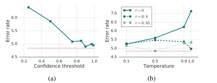
Figure 3: Plots of ablation studies on FixMatch. (a) Varying the confidence threshold for pseudo-labels. (b) Measuring the effect of “sharpening” the predicted label distribution while varying the confidence threshold (). Error rate of FixMatch with default hyperparameters is in red dotted line.
图 3:FixMatch 消融实验曲线。(a) 改变伪标签的置信度阈值。(b) 在改变置信度阈值()的同时,测量对预测标签分布做“锐化”的影响。红虚线是默认超参数下 FixMatch 的错误率。
| Ablation | Error |
|---|---|
| FixMatch | 4.84 |
| Only Cutout | 6.15 |
| No Cutout | 6.15 |
Table 3: Ablation study with different strong data augmentation of FixMatch. Error rates are reported on a single 250-label split from CIFAR-10.
| 消融设置 | 错误率 |
|---|---|
| FixMatch | 4.84 |
| 仅 Cutout | 6.15 |
| 无 Cutout | 6.15 |
表 3:FixMatch 不同强数据增强的消融。错误率在 CIFAR-10 的单个 250 标签划分上报告。
5.1 Sharpening and Thresholding
5.1 锐化与阈值
A “soft” version of pseudo-labeling can be designed by sharpening the predicted distribution. This formulation appears in UDA and is of general interest since other methods such as MixMatch and ReMixMatch also make use of sharpening (albeit without thresholding). Using sharpening instead of an introduces a hyper-parameter: the temperature [4, 54, 3].
也可以通过对预测分布做锐化,得到伪标签的“软”版本。这一写法出现在 UDA 中,并且有一般意义,因为 MixMatch、ReMixMatch 等方法也使用锐化(只是没有阈值)。用锐化代替 会引入一个超参数:温度 [4, 54, 3]。
We study the interactions between the temperature and the confidence threshold . Note that pseudo-labeling in FixMatch is recovered as . The results are presented in fig. 3a and fig. 3b. The threshold value of 0.95 shows the lowest error rate, though increasing it to 0.97 or 0.99 did not hurt much. In contrast, accuracy drops by more than 1.5% when using a small threshold value. Note that the threshold value controls the trade-off between the quality and the quantity of pseudo-labels. As discussed in appendix B.2, the accuracy of pseudo-labels for unlabeled data increases with higher threshold values, while the amount of unlabeled data contributing to in eq. (4) decreases. This suggests that the quality of pseudo-labels is more important than the quantity for reaching a high accuracy. Sharpening, on the other hand, did not show a significant difference in performance when a confidence threshold is used. In summary, we observe that swapping pseudo-labeling for sharpening and thresholding would introduce a new hyperparameter while achieving no better performance.
我们研究温度 与置信度阈值 之间的相互作用。注意,当 时即回到 FixMatch 中的伪标签。结果见图 3a 和图 3b。阈值为 0.95 时错误率最低,提到 0.97 或 0.99 也不会差多少。相反,阈值较小时,准确率会下降超过 1.5%。阈值控制的是伪标签质量与数量之间的取舍。如附录 B.2 所讨论,阈值越高,无标注数据上伪标签的准确率越高,但能进入式 (4) 中 的无标注数据量会减少。这表明,要想达到高准确率,伪标签的质量比数量更重要。另一方面,在已经使用置信度阈值时,锐化并没有带来显著的表现差异。总的来看,若用“锐化加阈值”替换伪标签,只会多引入一个超参数,却并不能得到更好的结果。
5.2 Augmentation Strategy
5.2 增强策略
We conduct an ablation study on different strong data augmentation policies as it plays a key role in FixMatch. Specifically, we chose RandAugment [11] and CTAugment [3], which have been used for state-of-the-art SSL algorithms such as UDA [54] and ReMixMatch [4] respectively. On CIFAR-10, CIFAR-100, and SVHN we observed highly comparable results between the two policies, whereas in STL-10 (table 2), we observe a significant gain by using CTAugment.
强数据增强策略在 FixMatch 中作用关键,我们对不同策略做了消融。具体选择了 RandAugment [11] 和 CTAugment [3],它们分别用于 UDA [54]、ReMixMatch [4] 等领先 SSL 算法。在 CIFAR-10、CIFAR-100 和 SVHN 上,两种策略的结果高度接近;而在 STL-10 上(表 2),使用 CTAugment 有明显收益。
We measure the effect of Cutout in table 3, which is used by default after strong augmentation in both RandAugment and CTAugment. We find that both Cutout and CTAugment are required to obtain the best performance; removing either results in a significant increase in error rate.
表 3 测量了 Cutout 的作用;RandAugment 和 CTAugment 默认都会在强增强之后加上 Cutout。我们发现,要取得最好结果,Cutout 和 CTAugment 都不可少,去掉任何一项都会使错误率明显上升。
We also study different combinations of weak and strong augmentations for pseudo-label generation and prediction (i.e., the upper and lower paths in fig. 1). When we replaced the weak augmentation for label guessing with strong augmentation, we found that the model diverged early in training. Conversely, when replacing weak augmentation with no augmentation, the model overfits the guessed unlabeled labels. Using weak augmentation in place of strong augmentation to generate the model's prediction for training peaked at 45% accuracy but was not stable and progressively collapsed to 12%, suggesting the importance of strong data augmentation. This observation is well-aligned with those from supervised learning [10].
我们还研究了伪标签生成与预测(即图 1 中的上、下两条通路)对弱、强增强的不同组合。若把用于猜标签的弱增强换成强增强,模型会在训练早期就发散。反过来,若把弱增强去掉、完全不增强,模型会过拟合这些猜出来的无标注标签。若用弱增强代替强增强来生成用于训练的模型预测,准确率最高能到 45%,但不稳定,并会逐渐塌到 12%,说明强数据增强很重要。这与监督学习中的观察一致 [10]。
6 Conclusion
6 结论
There has been rapid recent progress in SSL. Unfortunately, much of this progress comes at the cost of increasingly complicated learning algorithms with sophisticated loss terms and numerous difficult-to-tune hyper-parameters. We introduce FixMatch, a simpler SSL algorithm that achieves state-of-the-art results across many datasets. We show how FixMatch can begin to bridge the gap between low-label semi-supervised learning and few-shot learning or clustering: we obtain surprisingly-high accuracy with just one label per class. Using only standard cross-entropy losses on both labeled and unlabeled data, FixMatch's training objective can be written in just a few lines of code.
半监督学习近来进展很快。可惜,其中不少进步是以学习算法越来越复杂为代价的:损失项精巧,超参数又多又难调。我们提出更简单的 SSL 算法 FixMatch,并在多个数据集上取得了当时最好的结果。我们也展示了它如何开始填补少标签半监督学习与少样本学习或聚类之间的间隙:每类只需一个标签,就能得到出人意料的高准确率。有标注和无标注数据都只用标准交叉熵,FixMatch 的训练目标只需几行代码就能写下来。
Because of this simplicity, we are able to thoroughly investigate how FixMatch works. We find that certain design choices are important (and often underemphasized) – most importantly, weight decay and the choice of optimizer. The importance of these factors means that even when controlling for model architecture as is recommended in [36], the same technique can not always be directly compared across different implementations.
正是因为简单,我们才能把 FixMatch 的工作机制查得比较清楚。我们发现,某些设计选择很重要(却常常被低估)——其中最突出的是权重衰减和优化器的选择。这些因素如此关键,意味着即便按 [36] 的建议控制了模型架构,同一技术在不同实现之间也未必能直接比较。
On the whole, we believe that the existence of such simple but performant semi-supervised machine learning algorithms will help to allow machine learning to be deployed in increasingly many practical domains where labels are expensive or difficult to obtain.
总体而言,我们相信这类既简单又好用的半监督机器学习算法,将有助于把机器学习推广到更多标签昂贵或难以获得的实际领域。
Broader Impact
更广泛的影响
FixMatch helps democratize machine learning in two ways: first, its simplicity makes it available to a wider audience, and second, its accuracy with only a few labels means that it can be applied to domains where previously machine learning was not feasible. The flip side of democratization of machine learning research is that it becomes easy for both good and bad actors to apply. We hope that this ability will be used for good—for example, obtaining medical scans is often far cheaper than paying an expert doctor to label every image. However, it is possible that more advanced techniques for semi-supervised learning will allow for more advanced surveillance: for example, the efficacy of our one-shot classification might allow for more accurate person identification from a few images. Broadly speaking, any progress on semi-supervised learning will have these same consequences.
FixMatch 从两方面让机器学习更容易普及:第一,它足够简单,能被更广泛的人使用;第二,只需很少标签就能达到可用准确率,因而可以进入从前难以应用机器学习的领域。普及的另一面是,善意和恶意的使用者都更容易把它用起来。我们希望这一能力被用在正当之处——例如,获取医学扫描往往远比请专业医生给每张图标注便宜。但更先进的半监督技术也可能被用于更强的监视:比如,我们在单样本分类上的效果,或许会让仅凭少量图像就能更准确地识别个人。广义上说,半监督学习的任何进展,都会带来同样的后果。
Funding Disclosure
资助声明
Google is the sole source of funding for this work.
本研究的唯一资助来源是 Google。
Acknowledgment
致谢
We thank Qizhe Xie, Avital Oliver, Quoc V. Le, and Sercan Arik for their feedback on this paper.
感谢 Qizhe Xie、Avital Oliver、Quoc V. Le 和 Sercan Arik 对本文的反馈。
References
参考文献
[1] E. Arazo, D. Ortego, P. Albert, N. E. O’Connor, and K. McGuinness. Pseudo-labeling and confirmation bias in deep semi-supervised learning. arXiv preprint arXiv:1908.02983, 2019. 5, 15
[2] P. Bachman, O. Alsharif, and D. Precup. Learning with pseudo-ensembles. In Advances in neural information processing systems, pages 3365–3373, 2014. 1, 3, 5
[3] D. Berthelot, N. Carlini, E. D. Cubuk, A. Kurakin, K. Sohn, H. Zhang, and C. Raffel. Remixmatch: Semi-supervised learning with distribution matching and augmentation anchoring. In Eighth International Conference on Learning Representations, 2020. 1, 2, 3, 4, 5, 6, 7, 8, 18, 19, 20, 21
[4] D. Berthelot, N. Carlini, I. Goodfellow, N. Papernot, A. Oliver, and C. A. Raffel. Mixmatch: A holistic approach to semi-supervised learning. In Advances in Neural Information Processing Systems, pages 5050–5060, 2019. 1, 2, 3, 5, 6, 7, 8, 14, 19
[5] N. Carlini, Ú. Erlingsson, and N. Papernot. Distribution density, tails, and outliers in machine learning: Metrics and applications. arXiv preprint arXiv:1910.13427, 2019. 7, 16
[6] O. Chapelle, B. Scholkopf, and A. Zien. Semi-Supervised Learning. MIT Press, 2006. 4
[7] J. Chen and Q. Gu. Closing the generalization gap of adaptive gradient methods in training deep neural networks. arXiv preprint arXiv:1806.06763, 2018. 15
[8] D. Choi, C. J. Shallue, Z. Nado, J. Lee, C. J. Maddison, and G. E. Dahl. On empirical comparisons of optimizers for deep learning. arXiv preprint arXiv:1910.05446, 2019. 15
[9] A. Coates, A. Ng, and H. Lee. An analysis of single-layer networks in unsupervised feature learning. In Proceedings of the Fourteenth International Conference on Artificial Intelligence and Statistics, 2011. 5
[10] E. D. Cubuk, B. Zoph, D. Mane, V. Vasudevan, and Q. V. Le. Autoaugment: Learning augmentation strategies from data. In The IEEE Conference on Computer Vision and Pattern Recognition (CVPR), June 2019. 4, 9, 20
[11] E. D. Cubuk, B. Zoph, J. Shlens, and Q. V. Le. Randaugment: Practical automated data augmentation with a reduced search space. arXiv preprint arXiv:1909.13719, 2019. 2, 4, 6, 7, 8, 18, 20
[12] Z. Dai, Z. Yang, F. Yang, W. W. Cohen, and R. R. Salakhutdinov. Good semi-supervised learning that requires a bad GAN. In Advances in Neural Information Processing Systems, 2017. 5
[13] J. Deng, W. Dong, R. Socher, L.-J. Li, K. Li, and L. Fei-Fei. ImageNet: A large-scale hierarchical image database. In IEEE Conference on Computer Vision and Pattern Recognition, 2009. 5
[14] T. DeVries and G. W. Taylor. Improved regularization of convolutional neural networks with cutout. arXiv preprint arXiv:1708.04552, 2017. 2, 4
[15] G. French, M. Mackiewicz, and M. Fisher. Self-ensembling for visual domain adaptation. In Sixth International Conference on Learning Representations, 2018. 4, 5
[16] P. Goyal, P. Dollár, R. Girshick, P. Noordhuis, L. Wesolowski, A. Kyrola, A. Tulloch, Y. Jia, and K. He. Accurate, large minibatch sgd: Training imagenet in 1 hour. arXiv preprint arXiv:1706.02677, 2017. 16
[17] Y. Grandvalet and Y. Bengio. Semi-supervised learning by entropy minimization. In Advances in neural information processing systems, 2005. 3, 5
[18] D. Hendrycks and K. Gimpel. A baseline for detecting misclassified and out-of-distribution examples in neural networks. arXiv preprint arXiv:1610.02136, 2016. 15
[19] D. Hendrycks, N. Mu, E. D. Cubuk, B. Zoph, J. Gilmer, and B. Lakshminarayanan. Augmix: A simple data processing method to improve robustness and uncertainty. arXiv preprint arXiv:1912.02781, 2019. 15
[20] J. Hestness, S. Narang, N. Ardalani, G. Diamos, H. Jun, H. Kianinejad, M. M. A. Patwary, Y. Yang, and Y. Zhou. Deep learning scaling is predictable, empirically. arXiv preprint arXiv:1712.00409, 2017. 1
[21] R. Jozefowicz, O. Vinyals, M. Schuster, N. Shazeer, and Y. Wu. Exploring the limits of language modeling. arXiv preprint arXiv:1602.02410, 2016. 1
[22] D. P. Kingma and J. Ba. Adam: A method for stochastic optimization. In Third International Conference on Learning Representations, 2015. 4
[23] A. Krizhevsky. Learning multiple layers of features from tiny images. Technical report, University of Toronto, 2009. 5
[24] S. Laine and T. Aila. Temporal ensembling for semi-supervised learning. In Fifth International Conference on Learning Representations, 2017. 1, 3, 5
[25] D.-H. Lee. Pseudo-label: The simple and efficient semi-supervised learning method for deep neural networks. In ICML Workshop on Challenges in Representation Learning, 2013. 1, 2, 3, 4, 5, 6
[26] K. Lee, K. Lee, H. Lee, and J. Shin. A simple unified framework for detecting out-of-distribution samples and adversarial attacks. In Advances in Neural Information Processing Systems, pages 7167–7177, 2018. 15
[27] S. Liang, Y. Li, and R. Srikant. Enhancing the reliability of out-of-distribution image detection in neural networks. arXiv preprint arXiv:1706.02690, 2017. 15
[28] I. Loshchilov and F. Hutter. SGDR: Stochastic gradient descent with warm restarts. In Fifth International Conference on Learning Representations, 2017. 4, 15
[29] I. Loshchilov and F. Hutter. Decoupled weight decay regularization. In Sixth International Conference on Learning Representations, 2018. 15
[30] D. Mahajan, R. Girshick, V. Ramanathan, K. He, M. Paluri, Y. Li, A. Bharambe, and L. van der Maaten. Exploring the limits of weakly supervised pretraining. In Proceedings of the European Conference on Computer Vision (ECCV), 2018. 1
[31] D. McClosky, E. Charniak, and M. Johnson. Effective self-training for parsing. In Proceedings of the main conference on human language technology conference of the North American Chapter of the Association of Computational Linguistics. Association for Computational Linguistics, 2006. 4
[32] G. J. McLachlan. Iterative reclassification procedure for constructing an asymptotically optimal rule of allocation in discriminant analysis. Journal of the American Statistical Association, 70(350):365–369, 1975. 1, 3, 4
[33] T. Miyato, S.-i. Maeda, S. Ishii, and M. Koyama. Virtual adversarial training: a regularization method for supervised and semi-supervised learning. IEEE transactions on pattern analysis and machine intelligence, 2018. 1, 3, 4, 5, 19
[34] Y. E. Nesterov. A method of solving a convex programming problem with convergence rate o(kˆ2). Doklady Akademii Nauk, 269(3), 1983. 4
[35] Y. Netzer, T. Wang, A. Coates, A. Bissacco, B. Wu, and A. Y. Ng. Reading digits in natural images with unsupervised feature learning. In NIPS Workshop on Deep Learning and Unsupervised Feature Learning, 2011. 5
[36] A. Oliver, A. Odena, C. A. Raffel, E. D. Cubuk, and I. Goodfellow. Realistic evaluation of deep semi-supervised learning algorithms. In Advances in Neural Information Processing Systems, pages 3235–3246, 2018. 2, 3, 5, 6, 9
[37] B. Oreshkin, P. R. López, and A. Lacoste. Tadam: Task dependent adaptive metric for improved few-shot learning. In Advances in Neural Information Processing Systems, pages 721–731, 2018. 7
[38] D. S. Park, W. Chan, Y. Zhang, C.-C. Chiu, B. Zoph, E. D. Cubuk, and Q. V. Le. Specaugment: A simple data augmentation method for automatic speech recognition. arXiv preprint arXiv:1904.08779, 2019. 19
[39] H. Pham and Q. V. Le. Semi-supervised learning by coaching. Submitted to the 8th International Conference on Learning Representations, 2019. https://openreview.net/forum?id=rJe04p4YDB. 5
[40] B. T. Polyak. Some methods of speeding up the convergence of iteration methods. USSR Computational Mathematics and Mathematical Physics, 4(5), 1964. 4
[41] A. Radford, J. Wu, R. Child, D. Luan, D. Amodei, and I. Sutskever. Language models are unsupervised multitask learners, 2019. 1
[42] C. Raffel, N. Shazeer, A. Roberts, K. Lee, S. Narang, M. Matena, Y. Zhou, W. Li, and P. J. Liu. Exploring the limits of transfer learning with a unified text-to-text transformer. arXiv preprint arXiv:1910.10683, 2019. 1
[43] A. Rasmus, M. Berglund, M. Honkala, H. Valpola, and T. Raiko. Semi-supervised learning with ladder networks. In Advances in Neural Information Processing Systems, 2015. 5, 6
[44] C. Rosenberg, M. Hebert, and H. Schneiderman. Semi-supervised self-training of object detection models. In Proceedings of the Seventh IEEE Workshops on Application of Computer Vision, 2005. 1, 4, 5
[45] M. Sajjadi, M. Javanmardi, and T. Tasdizen. Mutual exclusivity loss for semi-supervised deep learning. In IEEE International Conference on Image Processing, 2016. 1, 3
[46] M. Sajjadi, M. Javanmardi, and T. Tasdizen. Regularization with stochastic transformations and perturbations for deep semi-supervised learning. In Advances in Neural Information Processing Systems, 2016. 1, 3, 5
[47] H. Scudder. Probability of error of some adaptive pattern-recognition machines. IEEE Transactions on Information Theory, 11(3), 1965. 1, 3, 4
[48] R. Sennrich, B. Haddow, and A. Birch. Improving neural machine translation models with monolingual data. arXiv preprint arXiv:1511.06709, 2015. 19
[49] N. Srivastava, G. Hinton, A. Krizhevsky, I. Sutskever, and R. Salakhutdinov. Dropout: a simple way to prevent neural networks from overfitting. The journal of machine learning research, 15(1), 2014. 5
[50] I. Sutskever, J. Martens, G. Dahl, and G. Hinton. On the importance of initialization and momentum in deep learning. In International conference on machine learning, 2013. 4
[51] A. Tarvainen and H. Valpola. Mean teachers are better role models: Weight-averaged consistency targets improve semi-supervised deep learning results. In Advances in neural information processing systems, 2017. 1, 3, 5, 6
[52] V. Verma, A. Lamb, J. Kannala, Y. Bengio, and D. Lopez-Paz. Interpolation consistency training for semi-supervised learning. arXiv preprint arXiv:1903.03825, 2019. 1
[53] A. C. Wilson, R. Roelofs, M. Stern, N. Srebro, and B. Recht. The marginal value of adaptive gradient methods in machine learning. In Advances in Neural Information Processing Systems, pages 4148–4158, 2017. 15
[54] Q. Xie, Z. Dai, E. Hovy, M.-T. Luong, and Q. V. Le. Unsupervised data augmentation for consistency training. arXiv preprint arXiv:1904.12848, 2019. 1, 2, 3, 4, 5, 6, 7, 8, 16, 20
[55] Q. Xie, M.-T. Luong, E. Hovy, and Q. V. Le. Self-training with noisy student improves imagenet classification. In Proceedings of the IEEE/CVF Conference on Computer Vision and Pattern Recognition, pages 10687–10698, 2020. 1, 4, 5
[56] S. Zagoruyko and N. Komodakis. Wide residual networks. In Proceedings of the British Machine Vision Conference (BMVC), 2016. 6
[57] X. Zhai, A. Oliver, A. Kolesnikov, and L. Beyer. S4l: Self-supervised semi-supervised learning. In The IEEE International Conference on Computer Vision (ICCV), October 2019. 7, 19
[58] G. Zhang, C. Wang, B. Xu, and R. Grosse. Three mechanisms of weight decay regularization. arXiv preprint arXiv:1810.12281, 2018. 15
[59] H. Zhang, M. Cisse, Y. N. Dauphin, and D. Lopez-Paz. MixUp: Beyond empirical risk minimization. arXiv preprint arXiv:1710.09412, 2017. 4, 5, 19
[60] X. Zhu. Semi-supervised learning literature survey. Technical Report TR 1530, Computer Sciences, University of Wisconsin – Madison, 2008. 4
[61] X. Zhu and A. B. Goldberg. Introduction to semi-supervised learning. Synthesis lectures on artificial intelligence and machine learning, 3(1), 2009. 4
[62] Y. Zou, Z. Yu, B. Vijaya Kumar, and J. Wang. Unsupervised domain adaptation for semantic segmentation via class-balanced self-training. In Proceedings of the European Conference on Computer Vision (ECCV), pages 289–305, 2018. 5
A Algorithm
A 算法
We present the complete algorithm for FixMatch in algorithm 1.
算法 1 给出 FixMatch 的完整算法。
Algorithm 1 FixMatch algorithm.
- Input: Labeled batch , unlabeled batch , confidence threshold , unlabeled data ratio , unlabeled loss weight .
- {Cross-entropy loss for labeled data}
- for to do
- {Compute prediction after applying weak data augmentation of }
- end for
- {Cross-entropy loss with pseudo-label and confidence for unlabeled data}
- return
算法 1 FixMatch 算法。
- 输入: 有标注批次 ,无标注批次 ,置信度阈值 ,无标注数据比例 ,无标注损失权重 。
- {有标注数据的交叉熵损失}
- for to do
- {对 做弱增强后计算预测}
- end for
- {对无标注数据使用带置信度的伪标签交叉熵损失}
- return
B Comprehensive Experimental Results
B 完整实验结果
B.1 Hyperparameters
B.1 超参数
As mentioned in section 4, we used almost identical hyperparameters of FixMatch on CIFAR-10, CIFAR-100, SVHN and STL-10. Note that we used similar network architectures for these datasets, except that more convolution filters were used for CIFAR-100 (WRN-28-8) to handle larger label space and more convolutions were used for STL-10 (WRN-37-2) to deal with larger input image size. Following the suggestion in [4], we doubled the weight decay parameter for WRN-28-8 to avoid overfitting. Here, we provide a complete list of hyperparameters in table 4. Note that we did ablation study for most of these hyperparameters in section 5 ( in section 5.1, in appendix B.5, lr and (momentum) in appendix B.3, and weight decay in appendix B.6).
如第 4 节所述,我们在 CIFAR-10、CIFAR-100、SVHN 和 STL-10 上使用几乎相同的 FixMatch 超参数。这些数据集上的网络架构也相近,只是 CIFAR-100 为应对更大的标签空间使用了更多卷积滤波器(WRN-28-8),STL-10 为应对更大的输入图像使用了更多卷积层(WRN-37-2)。按 [4] 的建议,我们对 WRN-28-8 把权重衰减参数加倍,以免过拟合。表 4 给出完整超参数列表。其中多数超参数已在第 5 节做了消融( 见 5.1 节, 见附录 B.5,学习率和动量 见附录 B.3,权重衰减见附录 B.6)。
| CIFAR-10 | CIFAR-100 | SVHN | STL-10 | |
|---|---|---|---|---|
| 0.95 | 0.95 | 0.95 | 0.95 | |
| 1 | 1 | 1 | 1 | |
| 7 | 7 | 7 | 7 | |
| 64 | 64 | 64 | 64 | |
| lr | 0.03 | 0.03 | 0.03 | 0.03 |
| 0.9 | 0.9 | 0.9 | 0.9 | |
| Nesterov | True | True | True | True |
| weight decay | 0.0005 | 0.001 | 0.0005 | 0.0005 |
Table 4: Complete list of FixMatch hyperparameters for CIFAR-10, CIFAR-100, SVHN and STL-10.
| CIFAR-10 | CIFAR-100 | SVHN | STL-10 | |
|---|---|---|---|---|
| 0.95 | 0.95 | 0.95 | 0.95 | |
| 1 | 1 | 1 | 1 | |
| 7 | 7 | 7 | 7 | |
| 64 | 64 | 64 | 64 | |
| 学习率 | 0.03 | 0.03 | 0.03 | 0.03 |
| 0.9 | 0.9 | 0.9 | 0.9 | |
| Nesterov | True | True | True | True |
| 权重衰减 | 0.0005 | 0.001 | 0.0005 | 0.0005 |
表 4:CIFAR-10、CIFAR-100、SVHN 和 STL-10 上 FixMatch 的完整超参数列表。
B.2 Trade-off between the Quality and the Quantity of Pseudo-Labels with Confidence
B.2 置信度下伪标签质量与数量的权衡
To better understand the role of thresholding in FixMatch, we present in table 5 two additional measurements along with the test set accuracy: the impurity (the error rate of unlabeled data that falls above the threshold) and the mask rate (the number of examples which are masked out) which are computed as follows:
为更好理解阈值在 FixMatch 中的作用,表 5 在测试集准确率之外还给出两项度量:杂质率(impurity,即超过阈值的无标注数据的错误率)和掩码率(mask rate,被掩掉的样本数量),计算如下:
| mask rate | impurity | error rate | |
|---|---|---|---|
| 0.25 | 100.00 | 6.39 | 6.40 |
| 0.5 | 100.00 | 5.40 | 5.87 |
| 0.75 | 99.82 | 5.35 | 5.09 |
| 0.85 | 99.31 | 4.32 | 5.12 |
| 0.9 | 99.21 | 3.85 | 4.90 |
| 0.95 | 98.13 | 3.47 | 4.84 |
| 0.97 | 96.35 | 2.30 | 5.00 |
| 0.99 | 92.14 | 2.06 | 5.05 |
Table 5: The mask rate and impurity at the end of the training along with the test set error rate of FixMatch using different threshold values on a single 250-label split from CIFAR-10.
| 掩码率 | 杂质率 | 错误率 | |
|---|---|---|---|
| 0.25 | 100.00 | 6.39 | 6.40 |
| 0.5 | 100.00 | 5.40 | 5.87 |
| 0.75 | 99.82 | 5.35 | 5.09 |
| 0.85 | 99.31 | 4.32 | 5.12 |
| 0.9 | 99.21 | 3.85 | 4.90 |
| 0.95 | 98.13 | 3.47 | 4.84 |
| 0.97 | 96.35 | 2.30 | 5.00 |
| 0.99 | 92.14 | 2.06 | 5.05 |
表 5:在 CIFAR-10 单个 250 标签划分上,使用不同阈值时,FixMatch 训练结束时的掩码率、杂质率以及测试集错误率。
As shown in table 5, when using small threshold values, most unlabeled examples' confidence is above the threshold. Consequently, they all contribute to the unlabeled loss in eq. (4). Unfortunately, pseudo-labels of these examples are not always correct and the learning process is significantly impeded by noisy pseudo-labeled examples. This behavior is known as confirmation bias [1]. On the other hand, using high threshold values allows a smaller fraction of ostensibly higher-quality unlabeled examples to contribute to the unlabeled loss, effectively reducing the confirmation bias with strong data augmentation, resulting in lower error rates on the test set. Given our observation on the trade-off between the quality and the quantity of pseudo-labels, combining improved techniques for confidence calibration and uncertainty estimation [18, 27, 26, 19] into FixMatch would be a promising future direction.
如表 5 所示,阈值较小时,绝大多数无标注样本的置信度都超过阈值,因而都会进入式 (4) 的无标注损失。可惜这些样本的伪标签并不总是正确,带噪声的伪标签会明显妨碍学习。这一现象被称为确认偏差 [1]。另一方面,使用高阈值时,只有较小一部分看起来质量更高的无标注样本会进入无标注损失;再配合强数据增强,能有效减轻确认偏差,从而降低测试集错误率。基于我们对伪标签质量与数量权衡的观察,把更好的置信度校准和不确定性估计技术 [18, 27, 26, 19] 接到 FixMatch 上,会是一个有前景的方向。
B.3 Ablation Study on Optimizer
B.3 优化器消融
While the study of different optimizers and their hyperparameters is seldom done in previous SSL works, we found that they can have a strong effect on performance. We present ablation results on optimizers in table 7. First, we studied the effect of momentum () for the SGD optimizer. We found that the performance is somewhat sensitive to and the model did not converge when is set too large. On the other hand, small values of still worked fine. When is small, increasing the learning rate improved the performance, though they are not as good as the best performance obtained with . Nesterov momentum resulted in a slightly lower error rate than that of standard momentum SGD, but the difference was not significant.
以往 SSL 工作很少系统比较不同优化器及其超参数,但我们发现它们对表现影响很大。表 7 给出优化器消融结果。首先考察 SGD 的动量 :表现对 有一定敏感,若 设得过大,模型便不能收敛;较小的 则仍可工作。当 较小时,提高学习率能改善表现,但仍不如 时的最好结果。Nesterov 动量比标准动量 SGD 的错误率略低,但差别并不显著。
As studied in [53, 29], we did not find Adam performing better than momentum SGD. While the best error rate of the model trained with Adam is only 0.53% larger than that of momentum SGD, we found that the performance was much more sensitive to the change of learning rate (e.g., increase in error rate by more than 8% when increasing the learning rate to 0.002) than momentum SGD. Additional exploration along this direction to make Adam more competitive includes the use of weight decay [29, 58] instead of weight regularization and a better exploration of hyperparameters [7, 8].
与 [53, 29] 的研究一致,我们并未发现 Adam 优于带动量的 SGD。用 Adam 训练时最好错误率只比动量 SGD 高 0.53%,但对学习率变化要敏感得多(例如把学习率提到 0.002,错误率会升高超过 8%)。若要让 Adam 更具竞争力,可以进一步探索用权重衰减 [29, 58] 代替 权重正则,并更充分地搜索超参数 [7, 8]。
| Optimizer | Hyperparameters | Error |
|---|---|---|
| SGD | , , Nesterov | 4.84 |
| SGD | , , Nesterov | 84.33 |
| SGD | , , Nesterov | 21.97 |
| SGD | , , Nesterov | 5.79 |
| SGD | , , Nesterov | 6.42 |
| SGD | , , Nesterov | 6.76 |
| SGD | , , Nesterov | 6.06 |
| SGD | , , Nesterov | 5.27 |
| SGD | , , Nesterov | 5.19 |
| SGD | , , Nesterov | 5.74 |
| SGD | , | 4.86 |
| Adam | , , | 29.42 |
| Adam | , , | 14.42 |
| Adam | , , | 15.44 |
| Adam | , , | 13.93 |
| Adam | , , | 7.35 |
| Adam | , , | 6.12 |
| Adam | , , | 5.95 |
| Adam | , , | 5.44 |
| Adam | , , | 5.37 |
| Adam | , , | 5.57 |
| Adam | , , | 7.90 |
Table 7: Ablation study on optimizers. Error rates are reported on a single 250-label split from CIFAR-10.
| 优化器 | 超参数 | 错误率 |
|---|---|---|
| SGD | , , Nesterov | 4.84 |
| SGD | , , Nesterov | 84.33 |
| SGD | , , Nesterov | 21.97 |
| SGD | , , Nesterov | 5.79 |
| SGD | , , Nesterov | 6.42 |
| SGD | , , Nesterov | 6.76 |
| SGD | , , Nesterov | 6.06 |
| SGD | , , Nesterov | 5.27 |
| SGD | , , Nesterov | 5.19 |
| SGD | , , Nesterov | 5.74 |
| SGD | , | 4.86 |
| Adam | , , | 29.42 |
| Adam | , , | 14.42 |
| Adam | , , | 15.44 |
| Adam | , , | 13.93 |
| Adam | , , | 7.35 |
| Adam | , , | 6.12 |
| Adam | , , | 5.95 |
| Adam | , , | 5.44 |
| Adam | , , | 5.37 |
| Adam | , , | 5.57 |
| Adam | , , | 7.90 |
表 7:优化器消融。错误率在 CIFAR-10 的单个 250 标签划分上报告。
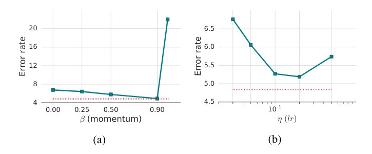
Figure 4: Plots of ablation studies on optimizers. (a) Varying . (b) Varying with .
图 4:优化器消融曲线。(a) 改变 。(b) 在 时改变 。
B.4 Ablation Study on Learning Rate Schedule
B.4 学习率日程消融
It is a popular choice in recent works [28] to use a cosine learning rate decay. As shown in table 6, a linear learning rate decay performed nearly as well. Note that, as for the cosine learning rate decay, picking a proper decaying rate is important. Finally, using no decay results in worse accuracy (a 0.86% degradation).
近期工作 [28] 常采用余弦学习率衰减。如表 6 所示,线性衰减的表现几乎同样好。需要注意的是,与余弦衰减一样,选对衰减幅度很重要。最后,不使用衰减会更差(准确率下降 0.86%)。
| Decay Schedule | Error |
|---|---|
| Cosine (FixMatch) | 4.84 |
| Linear Decay (end 0.01) | 4.95 |
| Linear Decay (end 0.02) | 5.55 |
| No Decay | 5.70 |
Table 6: Ablation study on learning rate decay schedules. Error rates are reported on a single 250-label split from CIFAR-10.
| 衰减日程 | 错误率 |
|---|---|
| 余弦(FixMatch) | 4.84 |
| 线性衰减(终点 0.01) | 4.95 |
| 线性衰减(终点 0.02) | 5.55 |
| 不衰减 | 5.70 |
表 6:学习率衰减日程消融。错误率在 CIFAR-10 的单个 250 标签划分上报告。
B.5 Ratio of Labeled to Unlabeled Data in Minibatch
B.5 小批次中有标注与无标注数据的比例
In fig. 5a we plot the error rates of FixMatch with different ratios of unlabeled data () in each minibatch. We observe a significant decrease in error rates by using a large amount of unlabeled data, which is consistent with the finding in UDA [54]. In addition, scaling the learning rate linearly with the batch size (a technique for large-batch supervised training [16]) was effective for FixMatch, especially when is small.
图 5a 画出了每个小批次中无标注数据比例()不同时 FixMatch 的错误率。使用大量无标注数据会显著降低错误率,这与 UDA [54] 的发现一致。此外,按批次大小线性缩放学习率 (这是大批次有监督训练中的做法 [16])对 FixMatch 也有效,尤其是在 较小时。
B.6 Weight Decay
B.6 权重衰减
While the value 0.0005 appeared as a good default choice for WRN-28-2 across datasets, we find that the weight decay could have a huge impact on performance when tuned incorrectly for low label regimes: choosing a value that is just one order of magnitude larger or smaller than optimal can cost ten percentage points or more, as shown in fig. 5b.
对 WRN-28-2 而言,0.0005 在各数据集上是不错的默认值;但在少标签情形下,权重衰减若调得不对,影响会非常大:只比最优点大或小一个数量级,就可能损失十个百分点甚至更多,见图 5b。
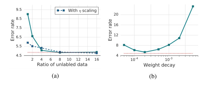
Figure 5: Plots of ablation studies on FixMatch. (a) Varying the ratio of unlabeled data () with different learning rate () scaling strategies. (b) Varying the loss coefficient for weight decay. Error rate of FixMatch with default hyperparameters is in red dotted line.
图 5:FixMatch 消融曲线。(a) 在不同学习率()缩放策略下改变无标注数据比例()。(b) 改变权重衰减的损失系数。红虚线是默认超参数下 FixMatch 的错误率。
B.7 Labeled Data for Barely Supervised Learning
B.7 极少监督学习中的有标注数据
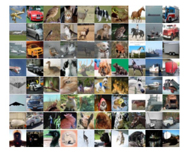
Figure 6: Labeled training data for the 1-label-per-class experiment. Each row corresponds to the complete labeled training set for one run of our algorithm, sorted from the most prototypical dataset (first row) to least prototypical dataset (last row).
图 6:每类 1 个标签实验所用的有标注训练数据。每一行对应一次算法运行的完整有标注训练集,从上到下按原型性从高到低排列(第一行最具原型性,最后一行最不具原型性)。
In addition to fig. 2, we visualize the full labeled training images obtained by ordering mechanism [5] used for barely supervised learning in fig. 6. Each row contains 10 images from 10 different classes of CIFAR-10 and is used as the complete labeled training dataset for one run of FixMatch. The first row contains the most prototypical images of each class, while the bottom row contains the least prototypical images. We train two models for each dataset and compute the mean accuracy between the two and plot this in fig. 7. Observe that we obtain over 80% accuracy when training on the best examples.
除图 2 外,图 6 可视化了按 [5] 的排序机制得到的、用于极少监督学习的全部有标注训练图像。每一行包含 CIFAR-10 中 10 个不同类别的 10 张图,作为一次 FixMatch 运行的完整有标注训练集。第一行是各类最具原型性的图像,最底行则是最不具原型性的图像。我们对每个数据集训练两个模型,取其平均准确率,并画在图 7 中。可以看到,用最好的样本训练时,准确率超过 80%。
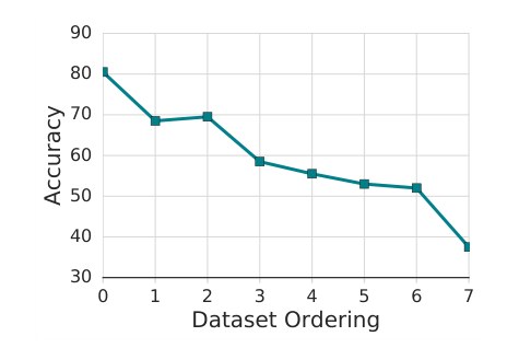
Figure 7: Accuracy of the model when trained on the 1-label-per-class datasets from Figure 6, ordered from most prototypical (top row) to least (bottom row).
图 7:在图 6 中每类 1 个标签的数据集上训练时模型的准确率,横轴按原型性从高(对应图 6 第一行)到低(最后一行)排列。
B.8 Comparison to Supervised Baselines
B.8 与有监督基线的比较
In table 9 and table 10, we present the performance of models trained only with the labeled data using strong data augmentations to highlight the effectiveness of using unlabeled data in FixMatch.
表 9 和表 10 给出了只用有标注数据、并采用强数据增强训练的模型表现,以凸显 FixMatch 利用无标注数据的效果。
| Dataset | 1 | 2 | 3 | 4 | 5 |
|---|---|---|---|---|---|
| CIFAR-10 | 5.46 | 6.17 | 9.37 | 10.85 | 13.32 |
| SVHN | 2.40 | 2.47 | 6.24 | 6.32 | 6.38 |
Table 8: Error rates of FixMatch (CTA) on a single 40-label split of CIFAR-10 and SVHN with different random seeds. Runs are ordered by accuracy.
| 数据集 | 1 | 2 | 3 | 4 | 5 |
|---|---|---|---|---|---|
| CIFAR-10 | 5.46 | 6.17 | 9.37 | 10.85 | 13.32 |
| SVHN | 2.40 | 2.47 | 6.24 | 6.32 | 6.38 |
表 8:FixMatch (CTA) 在 CIFAR-10 和 SVHN 的单个 40 标签划分上、使用不同随机种子的错误率。各次运行按准确率排序。
| Method | CIFAR-10 40 labels | CIFAR-10 250 labels | CIFAR-10 4000 labels | CIFAR-100 400 labels | CIFAR-100 2500 labels | CIFAR-100 10000 labels | SVHN 40 labels | SVHN 250 labels | SVHN 1000 labels |
|---|---|---|---|---|---|---|---|---|---|
| Supervised (RA) | |||||||||
| Supervised (CTA) | |||||||||
| FixMatch (RA) | |||||||||
| FixMatch (CTA) |
Table 9: Error rates for CIFAR-10, CIFAR-100 and SVHN on 5 different folds. Models with (RA) uses RandAugment [11] and the ones with (CTA) uses CTAugment [3] for strong-augmentation. All models are tested using the same codebase.
| 方法 | CIFAR-10 40 标签 | CIFAR-10 250 标签 | CIFAR-10 4000 标签 | CIFAR-100 400 标签 | CIFAR-100 2500 标签 | CIFAR-100 10000 标签 | SVHN 40 标签 | SVHN 250 标签 | SVHN 1000 标签 |
|---|---|---|---|---|---|---|---|---|---|
| Supervised (RA) | |||||||||
| Supervised (CTA) | |||||||||
| FixMatch (RA) | |||||||||
| FixMatch (CTA) |
表 9:CIFAR-10、CIFAR-100 和 SVHN 在 5 个不同折上的错误率。带 (RA) 的模型强增强使用 RandAugment [11],带 (CTA) 的使用 CTAugment [3]。所有模型都在同一套代码库上测试。
| Method | Error rate | Method | Error rate |
|---|---|---|---|
| Supervised (RA) | FixMatch (RA) | ||
| Supervised (CTA) | FixMatch (CTA) |
Table 10: Error rates for STL-10 on 1000-label splits. All models are tested using the same codebase.
| 方法 | 错误率 | 方法 | 错误率 |
|---|---|---|---|
| Supervised (RA) | FixMatch (RA) | ||
| Supervised (CTA) | FixMatch (CTA) |
表 10:STL-10 在 1000 标签划分上的错误率。所有模型都在同一套代码库上测试。
C Implementation Details for Section 4.3
C 第 4.3 节的实现细节
For our ImageNet experiments we use standard ResNet50 pre-activation model trained in a distributed way on a TPU device with 32 cores. We report results over five random folds of labeled data. We use the following set of hyperparameters for our ImageNet model:
ImageNet 实验使用标准的预激活 ResNet50,在 32 核 TPU 上分布式训练。结果在五个随机的有标注数据折上报告。ImageNet 模型使用如下超参数:
Batch size. On each step our batch contains 1024 labeled examples and 5120 unlabeled examples.
批次大小。每一步的批次包含 1024 个有标注样本和 5120 个无标注样本。
Training time. We train our model for 300 epochs of unlabeled examples.
训练时长。我们按无标注样本计算,训练 300 个 epoch。
Note that one epoch of unlabelled examples contains all 1.2 million examples from Imagenet training set and it correspond to 10 passes through labelled set for 10% Imagenet task.
注意,无标注样本的一个 epoch 包含 ImageNet 训练集中全部 120 万个样本;在使用 10% 有标注数据的 ImageNet 任务中,这相当于对有标注集合遍历 10 次。
Learning rate schedule. We utilize linear learning rate warmup for the first 5 epochs until it reaches an initial value of 0.4. Then we the decay learning rate at epochs 60, 120, 160, and 200 epoch by multiplying it by 0.1.
学习率日程。前 5 个 epoch 做线性预热,直到学习率达到初始值 0.4。随后在第 60、120、160 和 200 个 epoch 将学习率乘以 0.1 进行衰减。
Optimizer. We use Nesterov Momentum optimizer with momentum 0.9.
优化器。使用动量为 0.9 的 Nesterov Momentum 优化器。
Exponential moving average (EMA). We utilize EMA technique with decay 0.999.
指数滑动平均(EMA)。使用衰减系数为 0.999 的 EMA。
FixMatch loss. We use unlabeled loss weight and confidence threshold in FixMatch loss.
FixMatch 损失。无标注损失权重取 ,置信度阈值取 。
Weight decay. Our weight decay coefficient is 0.0003. Similarly to other datasets we perform weight decay by adding penalty of all weights to model loss.
权重衰减。系数为 0.0003。与其他数据集一样,我们把全部权重的 惩罚加到模型损失中来实现权重衰减。
Augmentation of unlabeled images. For strong augmentation we use RandAugment with random magnitude [11]. For weak augmentation we use a random horizontal flip.
无标注图像的增强。强增强使用带随机幅度的 RandAugment [11];弱增强使用随机水平翻转。
ImageNet preprocessing. We randomly crop and rescale to size all labeled and unlabeled training images prior to performing augmentation. This is considered a standard ImageNet preprocessing technique.
ImageNet 预处理。在做增强之前,对所有有标注和无标注训练图像随机裁剪并缩放到 。这是标准的 ImageNet 预处理做法。
D Extensions of FixMatch
D FixMatch 的扩展
D.1 Augmentation Anchoring and Distribution Alignment
D.1 增强锚定与分布对齐
Augmentation Anchoring, where strong augmentations are applied to each unlabeled example for consistency regularization, and Distribution Alignment, which encourages the model predictions to have same class distribution as the labeled set, are two important techniques to the success of ReMixMatch [3]. Thanks to its simplicity and clean formulation, incorporating these techniques into FixMatch becomes straightforward. Firstly, we incorporate Augmentation Anchoring into FixMatch as follows:
增强锚定对每个无标注样本施加 次强增强以做一致性正则;分布对齐则鼓励模型预测与有标注集合具有相同的类别分布。这两项技术对 ReMixMatch [3] 的成功很重要。由于 FixMatch 形式简单清楚,把它们接进来并不困难。首先,把增强锚定写入 FixMatch 如下:
Note that the strong augmentation is a stochastic process and it produces different strongly-augmented examples of an unlabeled example . Using and , FixMatch (CTA) with Augmentation Anchoring reduces the error rate averaged over 5 different folds on CIFAR-10 with 250 labeled examples from 5.07% to 4.81%.
注意强增强 是随机过程,会对同一个无标注样本 产生 个不同的强增强样本。取 、 时,带增强锚定的 FixMatch (CTA) 把 CIFAR-10、250 个有标注样本上 5 折平均错误率从 5.07% 降到 4.81%。
As already reported in section 4.1, combining Distribution Alignment into FixMatch improves the SSL performance significantly, especially when the number of labeled training data is very limited. Specifically, we align the predictive distribution of a weakly-augmented example using the dataset's marginal class distribution estimated using the labeled data and the running average of the model's prediction estimated by the unlabeled data as follows:
如 4.1 节已报告的,把分布对齐接到 FixMatch 上会显著改善半监督表现,在有标注训练数据非常有限时尤其明显。具体做法是:用有标注数据估计的数据集边际类别分布,以及由无标注数据估计的模型预测滑动平均,去对齐弱增强样本的预测分布 :
where . Now, eq. (4) can be modified as follows accordingly:
其中 。于是式 (4) 可相应改写为:
FixMatch (CTA) with distribution alignment reduces the error rate averaged over 5 different folds on CIFAR-10 with 40 labeled examples from 11.38% to 9.47%. On CIFAR-100 with 400 labeled examples, it reduces the error rate from 49.95% to 40.14%, which is also lower than 44.28% of ReMixMatch. In addition to Section 4.3, we conduct SSL experiments on ImageNet using 1% of its data as labeled examples. We find that in this regime the role of distribution alignment becomes more critical – FixMatch model does not train well without distribution alignment. On the other hand, after a proper tuning of hyperparameters (weight of unlabeled loss and confidence threshold ), FixMatch (RA) model with distribution alignment achieves 67.1% top-1 and 47.7% top-5 error rate (this correspond to 32.9% top-1 and 52.3% top-5 accuracy and similar to [57] results).
带分布对齐的 FixMatch (CTA) 把 CIFAR-10、40 个有标注样本上 5 折平均错误率从 11.38% 降到 9.47%;在 CIFAR-100、400 个有标注样本上,错误率从 49.95% 降到 40.14%,也低于 ReMixMatch 的 44.28%。除 4.3 节外,我们还在只用 1% ImageNet 数据作为有标注样本的设定下做了半监督实验。这一设定中分布对齐更加关键——没有它,FixMatch 模型训练不好。而在适当调整超参数(无标注损失权重 ,置信度阈值 )之后,带分布对齐的 FixMatch (RA) 达到 67.1% 的 top-1 错误率和 47.7% 的 top-5 错误率(对应 32.9% 的 top-1 准确率和 52.3% 的 top-5 准确率,与 [57] 的结果相近)。
D.2 Datatype-Agnostic Data Augmentation
D.2 与数据类型无关的数据增强
Strong augmentation plays a key role in FixMatch. Applying FixMatch to different problem domains than vision thus requires one to come up with a novel augmentation strategy. While there are domain-specific data augmentation strategies for different application domains, such as back-translation [48] for text classification or SpecAugment [38] for speech recognition, it is desirable if FixMatch can also be combined with datatype-agnostic data augmentation methods.
强增强在 FixMatch 中作用关键。若要把 FixMatch 用到视觉以外的问题领域,就需要想出新的增强策略。不同应用领域已有各自的增强方法,例如文本分类中的回译 [48],或语音识别中的 SpecAugment [38];若 FixMatch 也能与数据类型无关的增强方法结合,会更加理想。
In this section, we consider two such augmentation schemes, namely MixUp [59] and Virtual Adversarial Training (VAT) [33], as a replacement of RandAugment or CTAugment in FixMatch for image classification. For MixUp, instead of mixing both input and label, we mixed random pairs of inputs only using to be more consistent with the data augmentation in FixMatch. For VAT, we used . We evaluated on CIFAR-10 with 250 labeled data protocol and report the mean and standard deviation over 5 different folds in table 11. We make comparisons of our FixMatch variants to MixMatch [4] and VAT [33]. The FixMatch variant with (input) MixUp obtained comparable error rates to MixMatch, while the variant with VAT achieved significantly lower error rates than VAT. This suggests the generality of the FixMatch's framework against different data augmentation strategies.
本节考虑两种这类增强:MixUp [59] 和虚拟对抗训练(VAT)[33],用它们替换 FixMatch 在图像分类中的 RandAugment 或 CTAugment。对 MixUp,为了更贴近 FixMatch 中的数据增强,我们只混合随机成对的输入、不混合标签,并取 。对 VAT,取 。我们在 CIFAR-10、250 个有标注样本的设定下评测,并在表 11 中报告 5 折的均值与标准差。对照对象是 MixMatch [4] 和 VAT [33]。使用(输入)MixUp 的 FixMatch 变体,错误率与 MixMatch 相当;使用 VAT 的变体,错误率则明显低于 VAT。这说明 FixMatch 这一框架对不同数据增强策略具有一定通用性。
| FixMatch + Input MixUp | MixMatch | FixMatch + VAT | VAT |
|---|---|---|---|
Table 11: Error rates for CIFAR-10 with 250 labeled examples on 5 different folds. All models are tested using the same codebase.
| FixMatch + 输入 MixUp | MixMatch | FixMatch + VAT | VAT |
|---|---|---|---|
表 11:CIFAR-10 在 250 个有标注样本、5 个不同折上的错误率。所有模型都在同一套代码库上测试。
E List of Data Transformations
E 数据变换列表
Given a collection of transformations (e.g., color inversion, translation, contrast adjustment, etc.), RandAugment randomly selects transformations for each sample in a mini-batch. As originally proposed, RandAugment uses a single fixed global magnitude that controls the severity of all distortions [11]. The magnitude is a hyperparameter that must be optimized on a validation set e.g., using grid search. We found that sampling a random magnitude from a pre-defined range at each training step (instead of using a fixed global value) works better for semi-supervised training, similar to what is used in UDA [54].
给定一组变换(例如颜色反转、平移、对比度调整等),RandAugment 会为小批次中的每个样本随机选择变换。按最初的提议,RandAugment 使用一个固定的全局幅度来控制所有扭曲的强度 [11]。该幅度是超参数,必须在验证集上优化,例如用网格搜索。我们发现,在每一步训练从预定义区间里随机采样幅度(而不是使用固定的全局值),更适合半监督训练,这与 UDA [54] 中的做法类似。
Instead of setting the transformation magnitudes randomly, CTAugment [3] learns them online over the course of training. To do so, a wide range of transformation magnitude values is divided into bins (as in AutoAugment [10]) and a weight (initially set to 1) is assigned to each bin. All examples are augmented with a pipeline consisting of two transformations which are sampled uniformly at random. For a given transformation, a magnitude bin is sampled randomly with a probability according to the (normalized) bin weights. To update the weights of the magnitude bins, a labeled example is augmented with two transformations whose magnitude bins are sampled uniformly at random. The magnitude bin weights are then updated according to how close the model's prediction is to the true label. Further details on CTAugment can be found in [3].
CTAugment [3] 并不随机设定变换幅度,而是在训练过程中在线学习。做法是:把较宽的幅度取值范围分成若干箱(与 AutoAugment [10] 类似),并为每个箱分配一个权重(初始为 1)。所有样本都经过由两个均匀随机采样的变换组成的流水线增强。对给定变换,再按(归一化后的)箱权重随机采样一个幅度箱。更新幅度箱权重时,对一个有标注样本施加两个变换,其幅度箱均匀随机采样,再根据模型预测与真实标签的接近程度更新各箱权重。CTAugment 的更多细节见 [3]。
We used the same sets of image transformations used in RandAugment [11] and CTAugment [3]. For completeness, we listed all transformation operations for these augmentation strategies in table 12 and table 13.
我们使用与 RandAugment [11] 和 CTAugment [3] 相同的图像变换集合。为完整起见,表 12 和表 13 列出了这些增强策略中的全部变换操作。
| Transformation | Description | Parameter | Range |
|---|---|---|---|
| Autocontrast | Maximizes the image contrast by setting the darkest (lightest) pixel to black (white). | ||
| Brightness | Adjusts the brightness of the image. returns a black image, returns the original image. | ||
| Color | Adjusts the color balance of the image like in a TV. returns a black & white image, returns the original image. | ||
| Contrast | Controls the contrast of the image. A returns a gray image, returns the original image. | ||
| Equalize | Equalizes the image histogram. | ||
| Identity | Returns the original image. | ||
| Posterize | Reduces each pixel to bits. | ||
| Rotate | Rotates the image by degrees. | ||
| Sharpness | Adjusts the sharpness of the image, where returns a blurred image, and returns the original image. | ||
| Shear_x | Shears the image along the horizontal axis with rate . | ||
| Shear_y | Shears the image along the vertical axis with rate . | ||
| Solarize | Inverts all pixels above a threshold value of . | ||
| Translate_x | Translates the image horizontally by pixels. | ||
| Translate_y | Translates the image vertically by pixels. |
Table 12: List of transformations used in RandAugment [11].
| 变换 | 说明 | 参数 | 范围 |
|---|---|---|---|
| Autocontrast | 把最暗(最亮)像素设为黑(白),以最大化图像对比度。 | ||
| Brightness | 调整图像亮度。 得到黑图, 返回原图。 | ||
| Color | 像电视机那样调整色彩平衡。 得到黑白图, 返回原图。 | ||
| Contrast | 控制图像对比度。 得到灰图, 返回原图。 | ||
| Equalize | 均衡图像直方图。 | ||
| Identity | 返回原图。 | ||
| Posterize | 把每个像素降到 位。 | ||
| Rotate | 将图像旋转 度。 | ||
| Sharpness | 调整图像锐度。 得到模糊图, 返回原图。 | ||
| Shear_x | 沿水平轴以比率 错切图像。 | ||
| Shear_y | 沿垂直轴以比率 错切图像。 | ||
| Solarize | 反转所有高于阈值 的像素。 | ||
| Translate_x | 将图像水平平移 个像素。 | ||
| Translate_y | 将图像垂直平移 个像素。 |
表 12:RandAugment [11] 使用的变换列表。
| Transformation | Description | Parameter | Range |
|---|---|---|---|
| Autocontrast | Maximizes the image contrast by setting the darkest (lightest) pixel to black (white), and then blends with the original image with blending ratio . | ||
| Brightness | Adjusts the brightness of the image. returns a black image, returns the original image. | ||
| Color | Adjusts the color balance of the image like in a TV. returns a black & white image, returns the original image. | ||
| Contrast | Controls the contrast of the image. A returns a gray image, returns the original image. | ||
| Cutout | Sets a random square patch of side-length pixels to gray. | ||
| Equalize | Equalizes the image histogram, and then blends with the original image with blending ratio . | ||
| Invert | Inverts the pixels of the image, and then blends with the original image with blending ratio . | ||
| Identity | Returns the original image. | ||
| Posterize | Reduces each pixel to bits. | ||
| Rescale | Takes a center crop that is of side-length , and rescales to the original image size using method . | , | , see caption |
| Rotate | Rotates the image by degrees. | ||
| Sharpness | Adjusts the sharpness of the image, where returns a blurred image, and returns the original image. | ||
| Shear_x | Shears the image along the horizontal axis with rate . | ||
| Shear_y | Shears the image along the vertical axis with rate . | ||
| Smooth | Adjusts the smoothness of the image, where returns a maximally smooth image, and returns the original image. | ||
| Solarize | Inverts all pixels above a threshold value of . | ||
| Translate_x | Translates the image horizontally by pixels. | ||
| Translate_y | Translates the image vertically by pixels. |
Table 13: List of transformations used in CTAugment [3]. The ranges for the listed parameters are discretized into 17 equal bins, except for the parameter of the Rescale transformation, which takes one of the following six options: anti-alias, bicubic, bilinear, box, hamming, and nearest.
| 变换 | 说明 | 参数 | 范围 |
|---|---|---|---|
| Autocontrast | 把最暗(最亮)像素设为黑(白)以最大化对比度,再按混合比 与原图混合。 | ||
| Brightness | 调整图像亮度。 得到黑图, 返回原图。 | ||
| Color | 像电视机那样调整色彩平衡。 得到黑白图, 返回原图。 | ||
| Contrast | 控制图像对比度。 得到灰图, 返回原图。 | ||
| Cutout | 把边长为 像素的随机正方形区域设为灰色。 | ||
| Equalize | 均衡图像直方图,再按混合比 与原图混合。 | ||
| Invert | 反转图像像素,再按混合比 与原图混合。 | ||
| Identity | 返回原图。 | ||
| Posterize | 把每个像素降到 位。 | ||
| Rescale | 取边长为 的中心裁剪,再用方法 缩放回原图尺寸。 | , | ,见图注 |
| Rotate | 将图像旋转 度。 | ||
| Sharpness | 调整图像锐度。 得到模糊图, 返回原图。 | ||
| Shear_x | 沿水平轴以比率 错切图像。 | ||
| Shear_y | 沿垂直轴以比率 错切图像。 | ||
| Smooth | 调整图像平滑度。 得到最平滑的图像, 返回原图。 | ||
| Solarize | 反转所有高于阈值 的像素。 | ||
| Translate_x | 将图像水平平移 个像素。 | ||
| Translate_y | 将图像垂直平移 个像素。 |
表 13:CTAugment [3] 使用的变换列表。所列参数的范围被离散成 17 个等宽箱,但 Rescale 变换的 参数除外,它取以下六种之一:anti-alias、bicubic、bilinear、box、hamming 和 nearest。